Geometric Methods for Two-Point Nonlinear Boundary Value ... · Geometric Methods for Two-Point Nonlinear Boundary Value Problems CARMEN CHICONE* ... 0 is always a solution. We are

JOURNAL OF DIFFERENTIAL EQUATIONS 72, 360-407 (1988)

Geometric Methods for Two-Point Nonlinear Boundary Value Problems

CARMEN CHICONE*

Department of Mathematics, University of Missouri, Columbia, Missouri 65211

Received August 7, 1986; revised June 5, 1987

1. INTRODUCTION

In the analysis of nonlinear boundary value problems there are two situations which often arise where general existence theorems do not easily apply and special techniques must be used. The first situation occurs when there is a trivial solution to the boundary value problem so that general existence theorems guarantee the existence of the trivial solution instead of a solution of interest which satisfies a side condition. The second situation occurs when growth in the derivative of the dependent variable is not bounded by a quadratic function in which case there may be no solution. The purpose of this paper is to make a contribution to the understanding of these problems especially for the class of differential equations of form

5? = F(Yc) + G(x)

with either Dirichlet (x(0) = 0, x(T) = 0) or Neumann (k(0) = 0, ~(T) = 0) boundary values.

The first situation is typified by the Neumann problem

5 ~ + # s i n x = 0

2~(0) = O, ~(T) = O,

where p > O. Here x - 0 is always a solution. We are interested in solutions where x ( t )= 0 exactly N times on [0, T), i.e., solutions with N nodes. If this problem is viewed geometrically the important features become immediately apparent. The phase flow has a stationary point at the origin which is surrounded by a continuous family of periodic trajectories whose

* Research supported in part by a grant from the Research Council of the Graduate School, University of Missouri.

360 0022-0396/88 $3.00 Copynght © 1988 by Academic Press, Inc All rights of reproduction m any form reserved

GEOMETRIC BOUNDARY VALUE PROBLEMS 361

FIG, 1. Typical Neumann situation.

outer boundary is a separatrix cycle. These periodic trajectories may be parametrized by choosing their initial values in the segment (0, rt) on the x-axis. A solution of our boundary value problem with N nodes corresponds to such a periodic phase trajectory with minimum period 2TIN. Taking into account the symmetry of the vector field in the phase plane with respect to the x-axis (which corresponds to the time reversibility of the differential equation, i.e., x(t) is a solution if and only if x ( T - t) is a solution), a moment of reflection reveals that the analysis of the boundary value problem can be completely understood in terms of the period function P, which assigns to each x e (0, n) the period of the phase trajectory with initial value (x, 0), and the limiting values of P at the end points of its interval of definition.

This example is a prototype problem which satisfies what we call the standard Neumann situation. Namely, the periods of the trajectories tend to the period of the linearized equations at the stationary point which is the inner boundary of the continuous family of periodic trajectories (in the example P(x)---~2~p -1/2 as x ~ 0 ) , the period function is monotone increasing on its domain (see, for example, [8]), and P(x) tends to infinity as x approaches the outer boundary of the family of periodic trajectories (in the example P(x) --* oo as x ~ rt). If the standard Neumann situation holds there is a solution of the Neumann problem with boundary values ~(0) = 0, ~(T)= 0 unique up to time reversal with N nodes if and only if the period of the linearized equations is smaller than 2TIN. Also, for fixed T there are only a finite number of solutions. This concept of the standard Neumann situation perhaps stated in different mathematical language is by now quite familiar. However, in general it remains a difficult problem to

362 CARMEN CHICONE

verify the key feature of the analysis which is the monotonicity of the period function.

Recently, a number of different authors [8, 10, 11, 20, 21, 22, 23, 24, 26, 27] have treated the general question of monotonicity but so far all of these efforts have been made in the special case when the phase flow is in Hamiltonian form. In particular this will be the case when the differential equation in the boundary value problem comes from a conservative Newtonian model so that it has form ~ = - f ( x ) (as in the above example). However, to treat our model equation 5~ = F(~)+ G ( x ) which is not in Hamiltonian form we will prove a new result on the monotonicity of the period function.

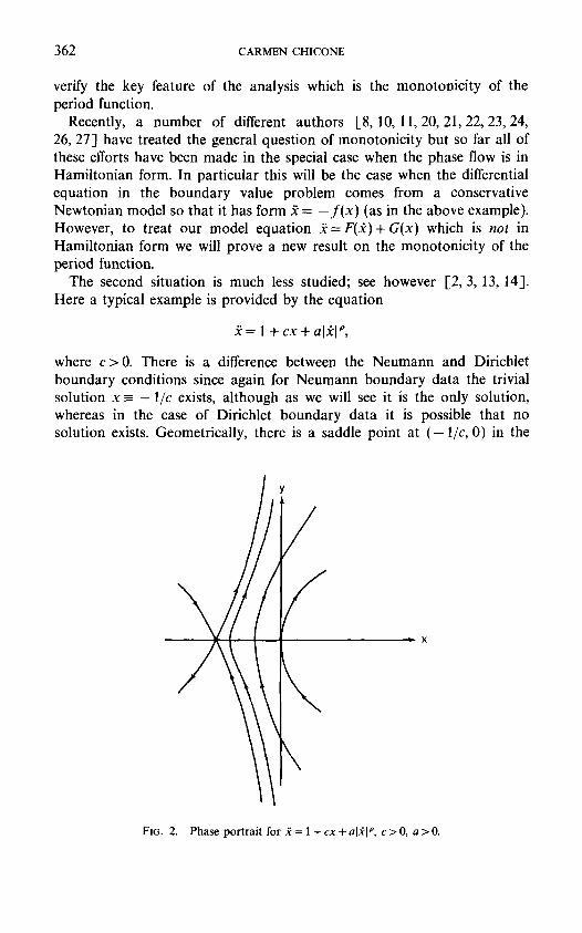
The second situation is much less studied; see however [2, 3, 13, 14]. Here a typical example is provided by the equation

~c = 1 + c x + alYcl p,

where c > 0. There is a difference between the Neumann and Dirichlet boundary conditions since again for Neumann boundary data the trivial solution x =- - l i e exists, although as we will see it is the only solution, whereas in the case of Dirichlet boundary data it is possible that no solution exists. Geometrically, there is a saddle point at ( - l / c , 0) in the

x

FIG. 2. Phase portrait for ~ = 1 +cx+a[Yc[ p, c > 0 , a > 0 .


phase plane and we have symmetry with respect to the x-axis. Taking into account the direction of the vector field on the x-axis and the fact that phase trajectories drift to the right above the x-axis and to the left below there is only one trajectory which starts and ends on the x-axis, namely, the trajectory corresponding to the stationary point x = - 1/c. So it is immediate that the Neumann problem has only the trivial solution. For the Dirichlet problem we must find a trajectory which starts on the negative :~ axis and returns to the ~ axis in exactly T units of time. As before the analysis is completely determined from knowledge of this "period function." In fact, the situation in the case c > 0, a > 0, and p ~> 2 is typical. The phase trajectories satisfy the system

~ = y

p= 1 +cx +aly[ p.

If we consider the family of all trajectories starting on the negative y-axis then the trajectory with initial value (0, 0) "returns" to the y-axis in zero units of time. If the function P: ( - ~ , 0 ) ~ R which assigns to each y e ( - ~ , 0) the time required for the trajectory starting at (0, y) to reach the positive y-axis (at (0, - y)) is monotone decreasing and if P(y) ~ L as y ~ - ~ , then the Dirichlet problem has a solution if and only if L > T, and this solution if it exists is unique. This is the standard Dirichlet situation.

We intend to center our analysis of the equation ~ = F ( ~ ) + G(x) with either Neumann or Dirichlet boundary values around the concept of the period function. In Section 2 we obtain a new result on the monotonicity of the period function when oscillations are present in the equation. Thus, we are able to state some conditions on F and G which ensure the standard Neumann situation. In Section 3 we consider the case when there are no oscillations and give some conditions which ensure the standard Dirichlet situation. In particular, we obtain an existence theorem for the Dirichlet problem similar in spirit (but different in point of view) to some results in [13]. In addition, we study the relationship between growth rates for F and the existence or nonexstence of solutions for the Dirichlet problem. This analysis illustrates geometrically the importance of a growth rate which is quadratic. In fact, if F(y)<~alyl p, 1 ~< p ~< 2 solutions always exist but for growth rates F(y)>~alyl p, p > 2 there are always choices for a above which there is no solution. The results of Section 3 lead to reasonably good estimates for the bifurcation value of a, for p > 2 fixed, where there is a transition from existence to nonexistence of solutions for the Dirichlet problem with x ( 0 ) = 0, x(T)= 0 for fixed T > 0. For example, in the test problem 5~ = 1 + x + al~[ 4, x ( 0 ) = 0, x(1 ) = 0 the bifurcation from existence to nonexistence occurs for a in the interval (24, 38).

364 CARMEN CHICONE

Throughout this paper we do not state the most general theorems nor do we consider all possible situations which can be treated by our methods. Rather we focus as clearly as possible on the geometric point of view and show applications to typical problems. As part of these illustrations we give a complete analysis of the Neumann and Dirichlet boundary value problems for the differential equation 2 = Ax2+ Bx + C. It is hoped that our methods will be applied in other situations as the need arises.

2. THE NEUMANN PROBLEM

In this section we prove a theorem on the monotonicity of the period function for the system of differential equation D given by

2 = - y

= x - xg(x) - yf(y)

in rectangular coordinates and by

-- - r sin 0 Q(r, O)

0 = 1 - cos 0 Q(r, 0),

where Q(r, 0) = cos 0 g(r cos 0) + sin 0 f ( r sin 0) in polar coordinates. The functions f and g are assumed to be C 2 functions on an interval I = ( - E , E) which satisfy

f ( - s ) = - f ( s ) , g ( - s ) = - g ( s ) , for s ~ I (1)

and f'(s)>~O, g'(s)>.O,f"(s)>.O, g"(s)>~O, for O<~s<E. (2)

To see that the conditions described above arise naturally in the analysis of the model equation 2 = F ( 2 ) + G(x) we note that in the presence of oscillations G will have the form G(x)= - f i x + xh(x). If we choose coordinates so that 2 = - x /~ Y we are led to a system of the form

2= - x / ~ Y

x + I-Z (x, y ).

The assumptions (1) and (2) ensure the origin is a center so the period function P is defined. Thus, (1) and (2) may be considered as assumptions about the form of the function H. Finally, since multiplication of the system of equations by f l - 1/2 does not affect the monotonicity of the period function but only changes each period by a constant multiple, this rescaling of the equations results in a system in the form D.


Before presenting our theorem we make a few easy observations about the system D. First, it is clear that D has a center at the origin of the phase plane. To see this note that the linearization near the origin has a center. Hence, trajectories starting sufficiently close to the origin "spiral" around the origin. But, the change of coordinates u = x, v = - y transforms D to the system

t i = V

0 = -- u + ug(u) + v f (v )

which after time reversal becomes

t i = - - v

f~ = u -- ug(u) -- v f (v) .

In other words the trajectories are symmetric with respect to the x-axis. It follows that any orbit which "spirals" aound the origin is periodic. Next, if f and g both vanish identically they will satisfy (I) and (2). Of course in this case the equations form a linear system which has a center at the origin such that the family of periodic trajectories surrounding the origin fills the entire phase plane. The period function P is defined on the entire positive x-axis and it has the constant value 2ft. In case at least one of the functions f and g is positive on (0, E), and both satisfy (1) and (2), consider the set of periodic trajectories surrounding the origin and the set A = { (r, 0):1 - c o s 0 Q(r, 0)>~ 0 } where the angular velocity is nonnegative. Clearly, A contains a neighborhood of the origin. We let (2 denote the region consisting of the continuous family of periodic trajectories whose inner boundary is the origin and such that £2 ~ A. Let J denote the set { x l ( x , O ) e £ 2 and x > 0 } and define P: J ~ R to be the period function which assigns to each x e J the minimum period of the trajectory of D starting at (x, 0). Also, define p: J ~ R to be the function which assigns to each x • J the minimum time required for the trajectory starting at (x, 0) to reach the negative x-axis. In our case, since we have the time reversal symmetry, P = 2p. However, it should be noted that, in general, the time required to reach the positive y-axis is not equal to one quarter of the period.

THEOREM 2.1. I f f , g sat is fy (1) and (2), then the func t ion p which

assigns to each x ~ J the m i n i mu m t ime required f o r a trajectory o f the dif ferential equation

Yc = - y

= x - x g ( x ) - y f ( y )

starting at (x, O) to reach the negative x -ax i s is monotone increasing on J.

3 6 6

Proof

Clearly

CARMEN CHICONE

We work with the system D in polar coordinates

- - - r s i n 0 Q(r, O)

0-- 1 - c o s 0 Q(r, 0).

dO p(x) = 1 - cos 0 Q(r(O, x), 0)'

where r(O, x) is the solution of the differential equation

dr - r sin 0 Q(r, O) - S(r, O)

dO 1 - c o s 0 Q(r, O)

with initial value r(O, x ) = x. Also,

oCOS 0 ( OQ/Or )( dr/Ox ) dO

We will show P'(x)> 0 for x e J. In order to estimate the sign of the derivative we consider in turn the

various factors in the integrand. First we compute an expression for dr/dx. In general, if

dr = S(r, O)

with r(0, x) = x, then dr/dx satisfies the variational equation

±(0q ds or dO \dx,I =-fir (r, O)--dx

with initial condition dr/dx (0, x) -- 1. The solution of this linear differential equation is

Or (0, x) = exp ~o dS d--'x Jo Or (r(% x), qg) de.

We can find a more useful from of this expression by the following observation,

Or r-~r S(r, ~o) + S(r, ~o)


SO

~r(r(qg'x)'q~)=r~-r(!S(r'q~)) + d

and therefore

o ~ 1 ° d I - - In x) &o ~S _~°r_~r(rS(r,q~))dqg+ r(q~, Io & dq~-Jo o dO

) = r S(r,q~) dqg+lnr(O,x)-lnr(O,x).

It follows that

) dr r(O, x) exp r S(r, q~) dq~ dx x

r(O, x) - - - E ( O , x ) .

X

We note that ~r/~x > 0 for x > 0. Now for x > 0 and fixed we substitute the formula just obtained for Or/dx

into the above formula for p'(x) to obtain

xp,(x)= fo~ r c°s O (OQ/Or) ~ dO (1 - cos 0 Q(r, 0)) "

Next, recall

Q(r, 0) = cos 0 g(r cos 0) + sin 0 f (r sin 0).

We have f ( 0 ) = 0, g ( 0 ) = 0 a n d f ' ( s ) / > 0, g'(s)>1 0 so both functions f and g are non negative for s > 0 and at least one of them is positive. This implies Q(r, 0) > 0 for 0 < 0 < n/2. For rt/2 < 0 < ~, sin 0 f (r sin 0) >/0 and since g ( - s ) = - g(s) both cos 0 and g(r cos 0) are nonpositive. Again, since at least one of the functions f and g is nonvanishing we have Q(r, 0) > 0 on re/2 < 0 < ft. Also,

0--~Q (r, 0) = cos20 g'(r cos 0) + sin2Of'(r sin 0) ~r

and we see that OQ/~r>~O on 0~<0<~rt. So, actually Q(r,O)>O and OQ/Or > 0 on 0 ~< 0 ~< n with the possible exceptions of the points 0 = 0, re/2, re.

505/72/2-12

368 CARMEN CHICONE

Returning to the integral expression for xp ' (x) we see the in tegrand is positive for 0 < 0 < ~r/2 and negative for 1r/2 < 0 < ~r. We must compare the integral over the interval [0, n /2 ] with the integral over the interval [~/2, it]. We have

f r cos 0 (dQ/Or) E(O) dO

(~/2 r(n - 8) cos 0 (OQ/Or)(r, zr - 8) E ( z - 8) dO

- --l.o ( l + c o s O Q ( r , g - O ) ) 2

Thus, the p roof will be complete when we show

r(O) cos 0 (OQ/Or)(r, 8) E(O) >>- r(n - 8) cos 0 (OQ/Or)(r, rt - 8) E(rt - 8)

(1 -- cos 0 Q(r, 8)) 2 (1 + cos 0 Q(r, lr - 8)) 2

for 0 < 0 < re/2. To this end note first that, since Q/> 0 on 0 ~< 0 ~< rr and since we are

assuming (r, 0) • A, we have

0~< l - c o s 0 Q(r, 8)~< 1 ~< 1 + c o s 0 Q(r, re -O)

for 0~<0~<rc/2. So,

1 1 (1 ~" cos 0 Q(r, 8)) 2 >~ (1 + cos 0 Q(r, lr - 8)) 2

for 0 ~< 0 ~< r~/2. Next we make a crucial observa t ion

dr - r s i n 0 Q ( r , O) <~0

dO 1 - c o s 0 Q(r, 8)

for 0 ~< 0 ~< 7r. Thus r is a nonincreasing function of 0 on this interval. In part icular

r(~--O) <~ r ( 2 ) <~ r(O)

for all Oe [0, re/2]. Since,

tgr9 v_~_~ (r, n - 8) = cos20g'( - r ( n - 8) cos 8) + sin2Of'(r(n - O) sin 8) Or

and g ' ( - s ) = g'(s) we have

~9_._Q_Q (r, rc - 8) = cos2Og'(r(rc - 8) cos 8) + sinZOf'(r(n - 8) sin 8). dr


But, g"(t)>~ 0 and f"(t)>~ 0 for t > O. Since r(rc- O)<~ r(O) for 0 ~ [0, rt/2] it follows that

OQ (r, O) >~ OQ ~ r - f i r ( r, ~ - O)

for all 0e [0, n/2]. To show the required inequality on the integrand we must show

E(O) >>. E ( n - 0). For this last inequality a straightforward calculation gives

OS r sin 0 (OQ/Or) sin 0 Q ---~(r, 0 ) = - ( l _ c o s 0 Q ) 2 1 - c o s 0 Q

r sin 0 (aQ/Or) 4_1 _ S(r, 0).

= (1 - c o s 0 Q ) 2 r

Now,

E ( 0 ) = e x p r-~r S(r, q2) dq)

f0 1 = exp jo - ~ r - r S d t p

f~ r sin tp (dQ/dr)(r, q)) = exp (1 - cos tp Q(r, ~0)) 2 &o.

But, the integrand in the integral just computed is nonpositive on the interval [0, re] and clearly E(O) is a nonincreasing function on [0, n]. Thus, E(O) >>. E(rc - O) for 0 ~ [0, rc/2] as required. |

One interesting and immediate corollary to Theorem 2.1 is obtained by setting f - 0 . This is a result which applies to certain vector fields which are Hamiltonian.

COROLLARY 2.2. I f g: (--E, E ) ~ R is a C 2 function which satisfies g ( - s ) = - g ( s ) for - E < s < E , g ' ( s ) > 0 for 0 < s < E , and g"(s)>>.O for 0 < s < E, then the differential equation 5i = - fix + xg(x) for fl > 0 has a monotone increasing period function. I f in addition g(E) >>. fl then the equation satisfies the standard Neumann situation.

Proof. The first statement is immediate from Theorem 2.1. To prove the second statement we have to examine the phase plane. Consider the system of equations in the phase variables which is

2~= - x / ~ Y x

370 CARMEN CHICONE

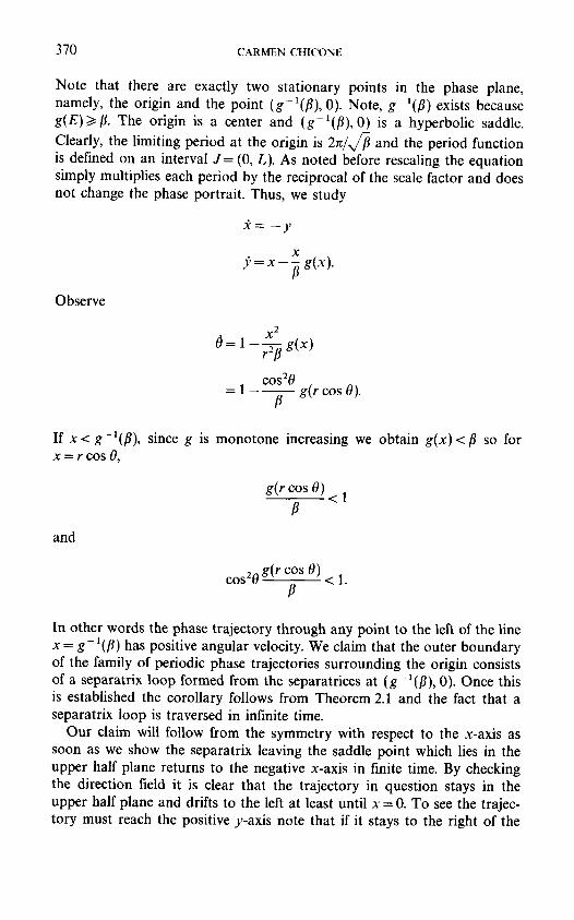
Note that there are exactly two stationary points in the phase plane, namely, the origin and the point (g-l(fl), 0). Note, g a(fl) exists because g ( E ) > ~ . The origin is a center and ( g - ~ ( f l ) , O ) is a hyperbolic saddle. Clearly, the limiting period at the origin is 2rc/x//-~ and the period function is defined on an interval J = (0, L). As noted before rescaling the equation simply multiplies each period by the reciprocal of the scale factor and does not change the phase portrait. Thus, we study

.¢c = -- y

X = x -- -~ g ( x ) .

Observe

X 2

cos20 = 1 - - - g ( r cos 0).

If x < g - ~ ( f l ) , since g is monotone increasing we obtain g ( x ) < fl so for X ---- r COS 0 ,

g ( r cos 0) <1

and

cos20 g ( r cos 0) < 1.

In other words the phase trajectory through any point to the left of the line x = g-~(fl) has positive angular velocity. We claim that the outer boundary of the family of periodic phase trajectories surrounding the origin consists of a separatrix loop formed from the separatrices at (g-~(fl), 0). Once this is established the corollary follows from Theorem 2.1 and the fact that a separatrix loop is traversed in infinite time.

Our claim will follow from the symmetry with respect to the x-axis as soon as we show the separatrix leaving the saddle point which lies in the upper half plane returns to the negative x-axis in finite time. By checking the direction field it is clear that the trajectory in question stays in the upper half plane and drifts to the left at least until x = 0. To see the trajectory must reach the positive y-axis note that if it stays to the right of the


y-axis its height increases with time. Thus once it reaches height 6 > 0 at time to, k < - f i for all later time. But then

x( t ) - X(to) < - 6(t - to)

so x ( t ) = 0 for some t < (X( to)+ 6to)/6. Similarly, the trajectory reaches its maximum height when x = 0 and then descends toward the negative x-axis. To see that the trajectory actually meets the x-axis note that once x(to) = - e < 0 we have

< - ~ / ~ - ~g(~)

and, as above, the trajectory reaches the t < to + y(to)/(e(fl + g(8))).

negative x-axis in time

EXAMPLE. The differential equation

f¢= - - f l x + x ( a j x + a 3 x 3 + ... +a2,v+lX2N+I), f l > 0 ,

where al , ..., a2N+l are nonnegative and at least one a , > O satisfies the standard Neumann situation. Other examples include

Y¢= -- flx + aixl e, f l > 0

for a > 0 , p~>2 and

~ = - f l x + a x t a n x , f l > 0

~ r a > 0 .

Returning to the not necessarily Hamiltonian case we now know when the differential equation 5~=F(Yc)+G(x) can be expressed in the form 5~ = - fix + xg (x ) + Ycf(Yc) where f and g satisfy hypotheses (1) and (2) of this section that the period function has the value 2~fl-1/2 at the origin and is monotone increasing. Thus, the differential equation will satisfy the standard Neumann situation provided the period function is unbounded. For our monotonicity theorem it was only necessary to have f and g defined in a neighborhood of the origin. However, in general, if the domain o f f or g is too small we cannot expect to have an unbounded period function. For simplicity we remove this concern in the next theorem.

TE1EOREM 2.3. For the differential equation

2 = G(x) + F(.~) = - fix + xg (x ) + Ycf(Yc), fl > 0

assume f and g satisfy (1) and (2) with both f and g defined on the whole real line. I f either sup(g(x): x>0}>~f l or sup(g(x): x > 0 } < f l and

372 CARMEN CHICONE

lim F ' ( F - I ( - G ( x ) ) ) = oo as x ~ ~ , then the differential equation has an unbounded period function. In particular, the differential equation satisfies the standard Neumann situation.

Proo f As before there is no loss in generality if we assume/~ = l and we study the system

Jc = - ),

y; = x - xg (x ) - y f ( y )

in the phase plane. Consider first the case when f vanishes and g satisfies (1) and (2). Each

phase trajectory is given as a level set of the Hamiltonian

y2 x

H(x , y ) = 2 - + fo s(1 - g ( s ) ) ds.

A trajectory starting at (A, 0), for A > 0 lies on the curve

fo' H(x , y) = s(1 - g(s)) ds.

If g(A) ~< 1 it is easy to see this curve crosses the negative x-axis. In fact, we only need to show

fo f0' - b s ( 1 - - g ( s ) ) d s = S(1 - g ( s ) ) d s

for some b > 0. But, there is such a b in the interval (0, A) since

a s ( l + g ( s ) ) d s > s ( l - g ( s ) ) d s ;

just change variables to s - + - s , remember g ( - s ) = - g ( s ) , g is nondecreasing, and g(0) = 0. Since all trajectories are symmetric with respect to the x-axis we have shown any trajectory starting at (A, 0), A > 0 with g(A) < 1 is periodic. Also, i f g (A)= 1, one checks that (A, 0) is a hyperbolic saddle point for the phase flow and we have just shown the separatrices to the left of this point form a homoclinic loop which in this case must be the outer boundary of the family of periodic trajectories surrounding the origin.

If f (y) does not vanish we have y f ( y ) >~ 0 for y ~> 0. But, then the trajectory for the system

2 = - y

= x - x g ( x ) - y f ( y )


starting at (A~ 0), A > 0 lies between the corresponding trajectory for the system

~ = - y

fi = x -- xg (x )

starting at the same point and the x-axis. It follows that the trajectory for the first system is periodic if the trajectory for the second system is periodic. Thus, if g ( A ) = 1 we have a saddle loop for both systems which is the outer boundary of the family of periodic trajectories surrounding the origin. If g ( x ) < 1 for all x > 0 all trajectories for both systems starting on the positive x-axis are periodic.

We must consider the periods of our periodic trajectories. In case g(A) = 1 the result follows immediately because the separatrix loop requires an infinite amount of time to be traversed. Thus, as periodic trajectories start close to this their outer boundary their periods become unbounded. We must make separate arguments for sup g < 1 and sup g- - 1.

If g(x) < 1 for all x > 0 we know all trajectories starting on the positive x-axis are periodic. The transit time for the trajectory starting at (A, 0) for A > 0 to reach the positive y-axis is given by

fA r = Jo y (x , A)"

If sup g = 1 observe that the trajectory for the same system with f identically zero attains its maximum when it reaches the y-axis. Since when f is not identically zero the trajectory lies below the corresponding trajectory for f equal to zero, we have in both cases ),,2

O<<.y(x,A)<~ 2 s ( 1 - g ( s ) ) d s

for O<~x<<.A. Thus

A 2 z2~>

2 ~g s(1 -- g(s)) ds"

To show the right hand side of the inequality is unbounded choose M > 0 . Since g ( s ) ~ 1 as s ~ ~ there is some choice for a > 0 such that ( 1 - g ( a ) ) - 1 > M. For any s > a we have 1 - g(s) < 1 - g(a), so for A > a

A 2 z2~> 2 ~g s(1 -- g(s)) ds + 2 ~a A S(I -- g(a)) as

A z 2 ~ s(1 - g(s)) ds + (1 - g(a)) A 2 - (1 - g(a)) a 2"

374 CARMEN CHICONE

For a chosen as above passing to the limit as A ~ oo we see z2> M as required.

Finally assume sup g < 1 but lim F ' ( F - I ( - G ( x ) ) ) = ~ as x ~ oo. We still have all trajectories starting on the positive x-axis periodic and the transit time to the y-axis for the trajectory starting at (A, 0) given by

~ dx

Y

Consider F and observe F ( y ) >10 for y > 0. Since lim F'(F- 1 ( - - G(x))) = ~ , F is eventually positive and thereafter F > 0. For simplicity we just assume F ' > 0 for y > 0. Now, dy/dx vanishes in the upper half plane on the curve y = h ( x ) = F - l ( x - x g ( x ) ) = F - l ( - G ( x ) ) . This curve starts at the origin and lies in the first quadrant . We claim h is nondecreasing. To see this compute for x > 0

1 - g(x) - xg'(x) h'(x) = F ' (F - l ( x - xg(x))

and observe it suffices to show (xg(x))'<~ 1 for x > 0. If this is not true there is some a > 0 with (ag(a)) '>tr> 1. Since g satisfies (2) we have (xg(x))" >10 and (xg(x))' > a for all x > a. But then, by integration,

ag(a) - ~ a

g(x) > + a X

for x > a. So there is some value of x such that g(x) > 1 cont rary to our assumption sup g < 1.

Now, returning to the trajectory starting at (A, 0), which drifts left in the upper half plane, we have

o < y(x, A) <~ h(A)

for O<.x<~A and, in turn, z>A/(h(A)) . If h(A) has a finite limit as A-- , ~ it is clear z ~ ~ . So suppose

h(A) ~ ~ as A ~ ~ . Applying L 'Hopi ta l ' s rule we consider the limit of 1/h'(A), i.e.,

F ' ( F - ' ( - G ( A ) ) )

1 - g ( A ) - A g ' ( A ) "

But, we have shown 0 ~< 1 - g ( A ) - Ag'(A) <~ 1. Since the numera to r tends to infinity with A the limit of the fraction is infinity and we have ~ ~ ~ as

A ~ . I


X

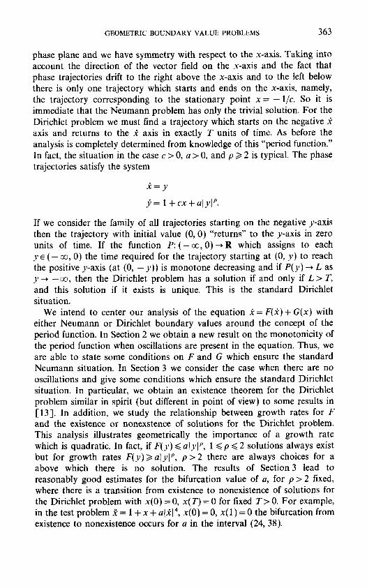
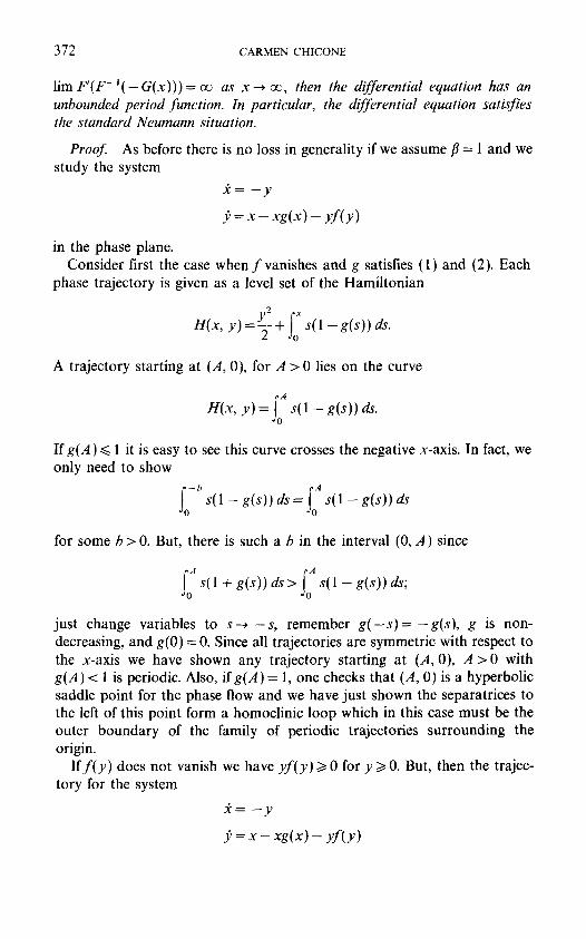
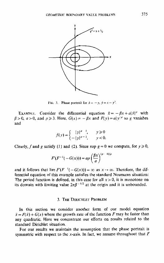
FIG. 3. Phase portrait for ~ = --y, ))= x - y2.

EXAMPLE. Consider the differential equation 5~=-flx+alYc[ ° with f l>0 , a > 0 , and p~>3. Here, G(x)= - f i x and F(y)=aly l p so g vanishes and

f ( y ) = f [ylp 1, y>~0 - l Y l "-~, y < 0 .

Clearly, f and g satisfy (1) and (2). Since sup g = 0 we compute, for y ~> 0,

F ' (F -~ (_G(x ) ) )=ap(~ -~ ) ¢p-I)/p

and it follows that lim F ' ( F - I ( - G ( x ) ) ) = oo as x--* ~ . Therefore, the differential equation of this example satisfies the standard Neumann situation: The period function is defined, in this case for all x > 0, it is monotone on its domain with limiting value 2nil-1/2 at the origin and it is unbounded.

3. THE DIRICHLET PROBLEM

In this section we consider another form of our model equation .~ = F(.¢c) + G(x) where the growth rate of the function F may be faster than any quadratic. Here we concentrate our efforts on results related to the standard Dirichlet situation.

For our results we maintain the assumption that the phase portrait is symmetric with respect to the x-axis. In fact, we assume throughout that F

376 CARMEN CHICONE

is a C ~ function defined on R satisfying F ( - s ) = F(s) and F(s) >~ 0 for s ~ 0. We note these restrictions imply F'(0) = 0. To obtain the Dirichlet situation we assume G is a C ~ function defined on R (although we do not need to know G for s > 0) which satisfies either

(1) G has no zero on ( - ~ , 0 ] , G ( s ) > 0 and G ' ( s ) > 0 on ( - o o , 0], o r

(2) G(L) = 0 for some L < 0 and G'(s) > 0 on (L, 0].

In case (2) holds we of course only consider solutions satisfying L <~ x(t) <~ O. (See the example following Corollary 3.3.)

Wth the above assumptions we consider the differential equation in the phase plane as the system

. ~ = y

~=G(x)+ F(y).

To solve the Dirichlet problem with boundary data x (0 )= 0, x(T)=0 we must find a phase trajectory starting on the negative y-axis which returns to the positive ),-axis in exactly time T. Under our assumptions phase trajectories drift left in the lower half plane and drift right in the upper half plane crossing the x-axis orthogonally. We have set up the equations so that the origin is not a stationary point. If the origin was a stationary point the corresponding trajectory is a trivial solution for the Dirichlet problem. In addition, under the hypotheses the right most stationary point on the negative x-axis which, if it exists, is at (L, 0), is a nondegenerate saddle point.

Now consider the phase trajectory starting at the origin. It starts on and returns to the y-axis in zero time. By continuity trajectories starting at (0, ~) for ~ < 0 and small also start on and return to the y-axis after crossing the negative x-axis transversally at some (fl, 0) for L < fl < 0. It might happen that some (0, ~) lies on a separatrix of the saddle point at (L, 0). This trajectory requires infinite time to reach the saddle point. So by continuity it is clear in this case that there will be a solution for the Dirichlet problem. If, on the other hand, a separatrix does not meet the negative y-axis all trajectories starting on the negative y-axis return to the positive y-axis in finite time and the Dirichlet problem has a solution if and only if the maximal time of return is larger than T. In either case the behavior of the function p(~) which assigns to a < 0 the time required for the trajectory starting at (0, ~) to reach the x-axis at (fl, 0) is decisive. Of course by the symmetry this function measures exactly half of the time required to reach the positive y-axis. As we have just seen p will be defined on some interval J = ( - A , 0] where possibly A = ~ . Also p(0) =0. To obtain the standard Dirichlet situation we need p'(~) < 0 on J and p(ct) ~ ~ as at ~ --A. Then

GEOMETRIC B O U N D A R Y VALUE PROBLEMS 377

the Dirichlet problem will always have a unique solution. We could also take T fixed and require both p'(~) < 0 on J and lim p(~) > T/2 as ~ --. - A .

Unlike the Neumann situation of Section 1, monotonicity for the Dirichlet situation is easy to prove.

PROPOSITION 3.1. Under the assumptions stated above the function p: J ~ R is monotone decreasing.

Proof In the phase plane we have

2 = y

= G(x) + F(y).

Consider trajectories starting at (0, ct), a < 0 which reach the negative x-axis at (~,0) with /~>L and observe for such trajectories )~>0. Moreover,

where x = x(y, ~t) satisfies

and

~o dy p(ct )

J~ G(x) + r (y ) '

dx y

dy G ( x ) + F ( y )

x(~, ~)=0

p'(ct) = G(x(ct, ct) ) + F(~)

f~C'(x)(~x/a~) dy. (G(x) + F(y)) 2

Since G'(x) > 0 for x(t) > L we will be finished with the proof as soon as we show ax/&t >~ O. But, ax/&t satisfies the variational equation

~ = (C(x)+ r (y ) ) ~ a~

SO

a~=~Z~ct,~)expfY --~'(x) 2dy aot Oct J, (G(x) + F(y)) "

Thus, the sign of ax/a~t is determined by the sign of ax/Oct(ot, at). To compute this, hold y = Y0 fixed and note that the phase trajectories starting at

378 CARMEN CHICONE

(0, ~), ~ < 0 cross the line y = Yo further to the right as ~ increases toward zero. It follows that Ox/&t (yo,~)>~0 and, in particular, 8x/O~ (~, ~)~>0. I

The interesting and more difficult part of the Dirichlet situation is to establish the limit of p(~) as ~ - ~ - - A . Of course one solution to this problem is to simply state the fact

fo dy lim p(c 0 = G(x) + F(y)

~x ~ - - A - - A

and observe the standard Dirichlet situation results if

f o dy T

-A G(x) + F(y) ~ 2"

However, in general, we cannot compute x(y, ct) or - A explicitly. So, in practice, the best one can hope for is an estimate of the integral. We can obtain an effective estimate using our hypotheses on F and G.

PROPOSITION 3.2. Assume ~ e J and the phase trajectory starting at (0, c~), ~ < 0 meets the negative x-axis at (fl, 0), then

o

f IG(O) + F(y) G([3) + F(y) _ ~ G(fl) + F(y)"

Proof Just observe x(y, ~) satisfies [3 <~ x(y, ~) <<. 0 for y e [~, 0]. As G' > 0 on [fl, 0] we have

O(O) + V(y) >>. G(x) + r ( y ) >1 G([3) + r ( y )

for y e [~, 0]. I

COROLLARY 3.3. The Diriehlet boundary value problem

Yc = F(Yc) + G(x)

x(O) = o, x ( r ) = o

with assumptions of this section on F and G has a unique solution if

0 d y ~ .

_~ G(O)+ F(y) 2

Proof First consider the case when G has a zero on the negative half line and suppose the stable separatrix of the corresponding saddle point in


the lower half of the phase plane meets the y-axis at (0, ~), ~ < 0. Since the time required for the trajectory starting at (0, a) to reach the saddle point is infinite whereas the time required for the trajectory starting at (0, 0) to reach the x-axis is zero as we have seen before there is some ~o e (~, 0) such that the trajectory starting at (0, ~0) reaches the negative x-axis in time exactly T/2. This solution is unique by Proposition 3.1.

If G has no zero or if the separatrix does not meet the negative y-axis there are two cases. In the first instance all trajectories starting on the negative ),-axis reach the negative x-axis in which case

o dy

f~ a(O) + F(y) <. p( oQ

for all 0~ by Proposition 3.2. Then, passing to the limit at a --, oo we have

T lim p(a) > 2"

On the other hand there may be a largest value - A such that the trajectory starting at (0, - A ) drifts to the left but never reaches the x-axis. Of course, this can only occur when G has no negative zero. In this case the time required for the trajectory starting at (0, - A ) to reach infinity is given by

y = >1 - - = o o . --y _~ A

It follows that for some c~ > - A there is a trajectory starting at (0, ~) which reaches the negative x-axis in exactly time T/2. |

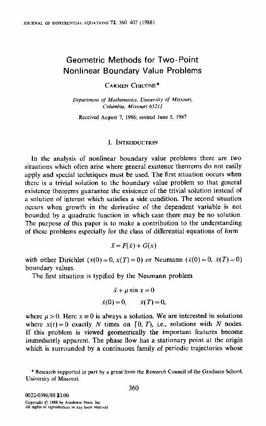
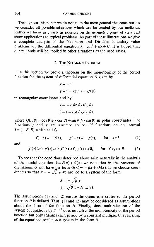
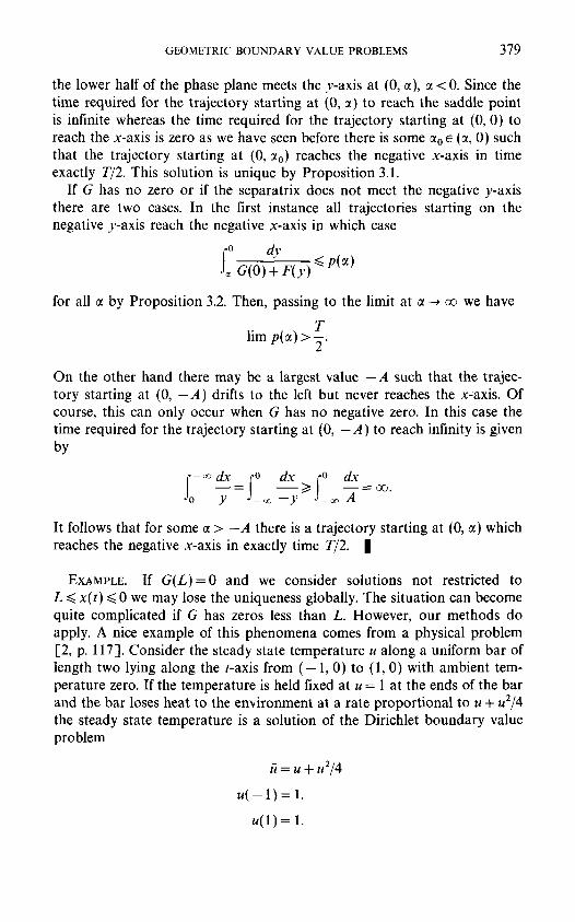
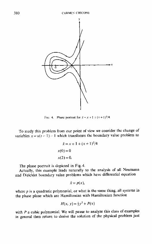
EXAMPLE. If G ( L ) = 0 and we consider solutions not restricted to L <<, x(t) <~ 0 we may lose the uniqueness globally. The situation can become quite complicated if G has zeros less than L. However, our methods do apply. A nice example of this phenomena comes from a physical problem [2, p. 117]. Consider the steady state temperature u along a uniform bar of length two lying along the t-axis from ( - 1, 0) to (1, 0) with ambient temperature zero. If the temperature is held fixed at u = 1 at the ends of the bar and the bar loses heat to the environment at a rate proportional to u + u2/4 the steady state temperature is a solution of the Dirichlet boundary value problem

i~ = u + u2/4

u ( - 1 ) = 1.

u(1)=1.

380 CARMEN CHICONE

Y

FIG. 4. Phase por t ra i t for 5~ = x + 1 + (x + 1)2/4.

To study this problem from our point of view we consider the change of variables x = u( t - 1 ) - 1 which transforms the boundary value problem to

57=x+ 1 + (x+ 1)2/4

x(O) = o

x(2)=o.

The phase portrait is depicted in Fig. 4. Actually, this example leads naturally to the analysis of all Neumann

and Dirichlet boundary value problems which have differential equation

~=p(x ) ,

where p is a quadratic polynomial, or what is the same thing, all systems in the phase plane which are Hamiltonian with Hamiltonian function

H(x, y) = ½y2 + P(x)

with P a cubic polynomial. We will pause to analyze this class of examples in general then return to derive the solution of the physical problem just

GEOMETRIC B O U N D A R Y VALUE PROBLEMS 381

stated as a special case. Although some of the analysis to follow is a con- sequence of the theory developed so far it is clear that a complete analysis must use special properties of the Hamiltonian. This will be evident as we proceed.

First, consider the Neumann problem. We can always translate the center to the origin so clearly it suffices to study the Hamiltonians of form

H(x , y ) = ½y2 + ax 2 + bx 3,

where a > O. Of course, if a < 0 we have a saddle at the origin and in the case a = 0 there is only one critical point which is not a center. If b = 0 the system is linear, so we consider b ¢ O. The differential equation

= - 2 a x - 3bx 2

for the Neumann boundary value problem for b > 0 with boundary conditions ~ (0 )=0 , k ( T ) = 0 satisfies the standard Neumann situation by a direct application of Corollary 2.2. The case b < 0 also satisfies the standard Neumann situation by the same corollary as is easily seen after the change of variables u = - x . Thus, the standard Neumann situation obtains for all problems with cubic Hamiltonian in the form given above with a > 0.

For the Dirichlet boundary value problem we consider the more general class of problems given by

5~ = A x 2 + B x + C

x(O) = D

x( T) = O

with A 4:0. We will give a rather complete analysis of this class of problems. Although we will actually prove more, the main proposition which we establish is the following.

The Dirichlet boundary value problem 5~ = A x 2 + B x + C, A ~ O, with

boundary values x(O)=D, x ( T ) = D with B 2 - 4 A C < ~ O has either no solutions, one solution or two solutions depending on the value o f T. In case

B 2 - 4 A C > O let x < x + denote the roots o f A x 2 + B x + C = O . Then, i f x < D < x+ ; there are a f in i te number o f solutions f o r each T with this number increasing to infinity as T ~ Go. I f either D <~ x _ or D >~ x +, there are either no solutions, one solution, or two solutions depending on the value

of 7 ~.

To simplify the calculations somewhat we will consider the equivalent boundary value problem obtained after the change of coordinates given by

U(t) = a2(Ax(~t) + 8/2),

382 CARMEN CHICONE

where

0"= I(B2--4AC)/4I 1/4, when B 2 - 4 A C ¢O

1, w h e n B 2 - 4AC= O.

This transforms our problem to

O = U Z + I

B U(O) = a2AD + -

2

where the plus sign is chosen when B 2 - 4 A C < 0 and the minus sign is chosen when B 2 - 4AC > 0; or to

t ) = g ~

B U(O) = AD +--

2

B U( T) = AD +-~,

when B 2 - 4 A C = O . By a change of notation we can therefore consider three cases,

2 = x 2, 2 = x 2+ 1, and 2 = x z - 1

with x(O) = d, x(T) = d.

Case 1. If 2 = x 2, the Hamiltonian is

1 yZ x3 H(x, y) = ~ 3

which has a degenerate critical point at the origin corresponding to a cuspoidal cubic when the energy E vanishes. Consider the line l given by x = d. To solve the Dirichlet problem we must compute the time required for a trajectory to pass from (d, - ~ ) to (d, ~), where ~ is the coordinate along l.

This transit time is given by an elliptic integral

q(~)= f , dy 2 f / dy _~ -Z =-~ (½ y2 _ E)2/3,

where, of course, E = ½cd - d3/3.


To begin, consider the cuspoidal cubic P

1 2 X3

- 3

which corresponds to two trajectories in the right half plane forming the separatrices (the stable and unstable manifolds) for the degenerate critical point at the origin. The line 1 meets P when d > 0. In this case we must consider the trajectories starting on 1 at points ( - a, d) which lie to the right of P, i.e., those trajectories with negative energy and also those trajectories which stay to the left of P, but cross the negative x-axis before returning to the line l.

For trajectories with negative energy the standard Dirichlet situation holds. To see this compute

, 2 4c~ ~ dy q ( c ~ ) = ~ + ~ - ~ I ° (ly2E)5/3

and observe that q ' (~)>0. Thus, our usual analysis holds as trajectories starting at (0, d) cross 1 in zero time, the transit time increases as increases, and as ( -ct, d) approaches the intersection of l and P, this transit time approaches infinity.

For the trajectories with positive energy the situation is more complicated. Assume first that d~<0 so for each ~ the trajectory through (d, - ~ ) has positive energy E. Recall,

E = ½e 2 - - ld3

and note

0 ~ 1 . x/ZE

Now, we make the change of variables y = x / / ~ sin 0 in the integral representation for q(~) and obtain

= @- E r d0 "~0 COS1/30"

When d = 0 this reduces, up to a positive constant multiple, to the integral

113 ~/2 dO O~

!~0 COS1/30"

So, in a sense, the standard Dirichlet situation holds: the time decreases from infinity, corresponding to the trivial solution at the critical point, to

505/72/2-13

384 CARMEN CHICONE

zero as ~ increases. Thus the Dirichlet problem has a unique solution for any T.

However, when d < 0 there may be one, two, or no solutions depending on T. To see this we compute q'(a) and obtain, up to a positive constant multiple,

i s m ~/.£T~) dO d - - ~ o [ E - 7/6

cosl/30 w/2 (3)1/3E ' ~0

Critical points of q' are solutions of the equation

~,~-q~/,f i~) dO 6 ( - d ) El l 6

cos"-----0 = (3 ) , /3

But, the integral is an increasing function of ~ and El/6ot 1 is a decreasing function of ~ so there is at most one critical point. Finally, it is easy to check q(0) = 0 and q(~) ~ 0 as a ~ oo so there is a critical point. Thus, for T near zero there are two solutions, when T = max q there is one solution and when T > max q there are no solutions.

When d > 0, the trajectory passes through the y-axis and the integral representation for q contains a singularity at

We split the integral into the convergent improper integrals over [0, . , 2 ~ ] and [ x / ~ , a] and make the change of variables y = x ~ sin 0 in the st integral and y = x / ~ sec 0 in the second integral thus obtaining

q(~)=2~92E_l/6(f£ec'(=/,/-~)__ sec0 dO+ f2= dO ) tanl/3--~ ~o cos-i?30 "

It is easy to check q(=) ~ 0 as a ~ m and q(a) + oo as a.~ (]d3) 1/2, i.e., as approaches the separatrix given by the cuspoidal cubic. Moreover, from the expression for q just obtained one can check that q is a decreasing function of ~. Thus the "standard" Dirichlet situation holds: the transit times are a monotone function of a and all the transit times are obtained. In particular, the Dirichlet boundary value problem always has a unique solution for any choice of T.

Case 2. If ~ = x 2 + 1, the level set of our Hamiltonian with energy E is given by

1 2 X3 ~y = ~ - + x + E


and the Hamiltonian system in the phase plane is

k = y

~ = X 2 + l .

Observe here that there are no stationary points for the flow and, using the integral, that each trajectory which meets the line x - d at (d, -0t), with c~ > 0, crosses the line again at (d, ~) after a transit time q given by

dx q(E) = 2 - - ,

o(E) Y

where xo(E) is the (unique) real root of

x 3 - - + x + E = 0 . 3

Clearly, q(E) is represented by a convergent improper integral. We are considering the trajectories meeting x = d as parametrized by E. But, since

~ 2 d3 = - ~ - + d + E

the parametrizations with respect to either E or ~ are easily related. We intend to show q is bounded, q(0)= 0, q ( ~ )= 0, and q has a unique

finite maximum value. Then, it follows that the Dirichlet boundary value problem

j~=X2+ 1

x(O ) = d ,x( T) = d

has either no solutions, one solution, or two solutions depending on T > m a x q , T = m a x q , or T < m a x q .

We have

dx

q(E) -~ x/~ ~o x/x3~3 + x + E"

Since Xo is a root of the cubic, the integral can be rewritten in the form

~/(x 3 - x3o)/3 + (x - Xo)'

386 CARMEN CHICONE

and since ( x - Xo)/>0, we can estimate q. In fact, dx

q( E) <<" x/~ J~,o ~

But, for Xo < 0 the change of variables x = Xo U gives

q ( E ) _ < _ _ ~ ~ 1 du

" xo J d,,o 4 1 - u;

and it follows easily that q(E)-+O as E--+oo. Just use x 0 - ) - o o as E-+ +oo.

When ~ = 0, xo(E)= d and q(E)= 0. Thus, to complete a proof of our claim it suffices to show q has at most one critical point. To do this requires using the algebraic structure inherent in the problem. We make an argument using the techniques related to the Picard-Fuch's equation from algebraic geometry, see [I0]. Since the analysis will also be used in Case 3 we study the Hamiltonian

where c = O, __+ 1. Define

1 ,~ X 3

~y '=T+cx+E,

Qo =2 1 y dx, O , = ~ xy dx

Io = -~ y dx, I, = o(el ocE) 2 xy dx

and observe, using prime for differentiation with respect to E, that since yy' = 1 we have

1 rd dx 1 1'o q(E). Jx0 , y

Also

I ; = ~ orE) Y

We seek a scalar differential equation for t'0. To this end compute

1 ( 2 ) d x x'/3+cX+Eax Qo = ~ y dx = y2 - - = Y Y

X 2 =~y(X + c - c ) dx+CX Y

X dy+2CX dx+E dx -57 y


and then

1 ~ 4 Io =.5 Io xdy+"sCI'l +2Ero.

But, an integration by parts yields

fo I/ x dy= x y l ; - y dx o

SO

Next compute

so that

5 4c , o~d "5 I° = T I1 "}- 2EI'o + T "

) Q1 Y y = - dX + y ~ -~ + c dx

x 2 2 cx 2 dx =eX +Ty + )dx y

= - - x 2 2c (x2+c'~ 2c 2 . EX dx + - ~ dy + dx---~y dX Y 3 k y ]

Ex x 2 2c 2c z =---f-- dx + - ~ dy +-~ dy - ~ y dX

4 2 l l o X 2 dy. I1 -- .5 c2I'o + 2EI'l + -5 ca + -5

Again, using an integration by parts we obtain

7 4c z 2 1 2 "511 = - --~ ro + 2 E l'l + -5 ca + 5 a d .

Thus, we have

( 2E 4c/3~(I'o~ 1 ( 5Io-o~d -4c2/3 2E J\l'~] =-5 \711 - ~(2c + d2)j"

Recall la2 = l d 3 + cd + E, so for a > 0

d~ 1 dE ct

388 CARMEN CHICONE

Next, differentiate the system of equations to obtain

( 2E 4c/31(I[~'l=~(,, l--I 'o--d/ot "~ --4c2/3 2E ]\I~'J - (2c + d2)/ot.]

and the "Picard-Fuch's" equation

4 ( I ~ = ( 2E "~ d \l'l'J 4c~/3

- 4 c / 3 1 ( ' -I 'o-d/o~ l 2E 1 \ I , - (2c + aa)/otJ

which holds for e > 0 with 3d = (9E2+ 4C3). Now we are able to obtain a differential equation for Io, namely

= 2Ed 4c(2c+a ¢)

4 3~

5 ed 2Ed 4c (2c+d 2) I F

- 3 °-t 3 ~ 30~

5 +2(d4 -- Io + 5cd 2 +4c 2 _ ~2d2).

We prefer to express this equation, PFI, in the form

dq' = - 51o + 2 (d 4 + 5cd2 q- 4c 2 _ ~2d)"

Finally, by differentiating, we obtain a scalar differential equation, PFII, for q;

dq" + d' q' = --~ q - (o~2d + dn + 5cd2 + 4c2).

We now return to our Dirichlet boundary value problem. We wish to show, in case c = 1, that q has exactly one critical point. To prove this we will show q ' < 0 whenever q'= O. Since A > 0, if q ' = 0, PFI gives

odd = - ~otlo + d 4 + 5cd 2 + 4¢ 2.

Upon substitution of this expression in PFII and a simple calculation we obtain the equation PFIII:

Aq" = -~-~3 (5~(cdI~ - Io) + 4(d 4 + 5cd 2 + 4c2)).


Moreover, as

and

fdo~ 2 d y ct2I'o - Io = Go 2y dx - fxo -2 dx

f~ l O~ 2 -- y2 = o ~ - - d x

y2 x 3 1 d 3

we have

d 3 ~2I'o- Io = Ix[ ~ (-~ + cd-X3

T -

B u t , for x < d a n d c = 1

d 3 x 3 ~+d--y-x>O

cx) dx.

and it follows immediately from PFIII that q " < 0 whenever q ' = 0 as required.

Case 3. When 5~ = x 2 - 1, we have

1 2 x3 -~ y = - ~ - x + E.

When E = 2, the corresponding level curve forms a saddle loop for the saddle point at (1, 0). This saddle loop encloses a center at ( - 1 , 0) and intersects the x-axis at ( - 2 , 0). We consider as usual the line given by x = d. However, there will be some subcases corresponding to the subsets bounded by the stable/unstable manifolds of the saddle point.

The first and easiest case, albeit the case which is often physically most important, is the case when d > l with the side condition l<<.x(t)<<.d. Geometrically, this case corresponds to the transit times of trajectories with energies less than 2. Of course, these are the trajectories which stay between the separatrices which lie to the right of the saddle point. For a given d > 1 we have the usual analysis as the transit time of the trajectory crossing the line x = d at (d, 0) is zero and the transit times grow monotonically to infinity as the trajectories cross x = d with energies approaching 2 from below. Of course, the transit times are unbounded because as E --. 2 the trajectories pass close to the saddle at (1, 0). The monotonicity follows from

390 CARMEN CHICONE

Proposition 3.1. For example, after the translation u = x - d we have F = 0 and G(s)= (s + d) 2 - 1. Thus, the Dirichlet boundary value problem for d > 1 with the side condition 1 <~ x(t)<~ d always has a unique solution.

Next, consider trajectories with energy larger then 2. For boundary conditions x ( 0 ) = d , x(T)=d we consider the transit time for a trajectory starting at (d, - ~ ) , in the lower half plane, to reach the point (d, ct) after crossing the x-axis at a point Xo < -2 . Such a trajectory remains outside the saddle loop corresponding to energy equal to ~-. Here ~ belongs to the interal [0, ~ ) for d~< - 2 and to the interval ( ( ~ ( d + 2 ) ( d - 1 ) z ) 1/2, ~ ) for d > -2 . As ~ approaches the left hand end point of its domain the transit time q is zero when d~< - 2 while for d > - 2 this transit time approaches the transit time along the separatrix of the saddle point. For d>~ 1 this time is infinite while for - 2 ~< d < 1 this transit time is given by

q = /2fax/'j dx =~/-21n x / - ~ 2 + x / ~ -2 x / (X+ 2 ) ( x - 1) 2 x / ~ 2 - x/~ "

We consider the subcases: - oo < d~< - 2 , - 2 < d < - 1 , and - 1 < d < ~ . For - 1 < d < ~ we intend to show q decreases monotonically to zero as

~ ~ . Thus, with E > 2 and 1 ~<d< ~ the Dirichlet boundary value problem has a unique solution while for - 1 < d < 1 there is a unique solution if and only if q(d) >1 T as given by the formula above. Of course, when d = 1 the constant solution corresponding to the saddle point, with energy ], is a trivial solution for the boundary value problem.

In order to show q decreases monotonically to zero we consider the time required to traverse the integral curve in the upper half plane from (Xo, 0) to (d, ~). This time is given by the sum of the two integrals

and

f a dx

l y

For q2 we have

fa dy/a~ dx q'z(a)= - 1 y2

But, clearly y(x, a) increases for fixed x as a increases. Thus t3y/Ox(x, ~) > 0 and q~(~)< 0. Moreover, the function y(x, ~) reaches its minimum height at x = 1. Since these minimums range to plus infinity it follows that q2(00 ~ 0 as ~ ~ ~ .


For ql(~) we consider the change of coordinates which translates the center to the origin and puts the linearization at the center in canonical form, i.e., the coordinates (u, v) given by

u = x / ~ ( x + 1)

v = y .

After a change to polar coordinates in the (u, v) plane we obtain our system in the form

/.2 i = ~- cos 2 0 sin 0

N//~ r O = - + ~ c o s 30 .

In these coordinates

and we compute

i~ : dO q l ( ~ ) = 2 /2 23/2 - r(O, ct) cos 3 0

U Or/Oa cos 3 0 dO q'l (o0 2 L /2 (2 3/2 - - r c o s 3 0 ) 2.

As Or/&t>O and cos 0 < 0 on re/2 < 0 < rt we have q'l(~) < 0. Moreover , we have

ql (xo)<2 f ~ dO .,~/2 2 3/2 + Xo COS 3 0"

Hence, ql(xo)--. 0 as xo ~ -Go. For d < - 1 we compute the transit time from (Xo, 0) to (d, ~) in polar

coordinates to obtain

f / dO q = 2 ,23/2 - r cos 3 0 '

where tan a = ~/(w/2 [ d + 11 )- Then, using the same estimate as made for q 1 above, it follows that q(Xo)~O as Xo ~ - ~ . Now, recall from our P ica rd -Fuch ' s computa t ion the equat ion P F I I I which in the present case, c = - 1, becomes

ct 3 dq" = -(5~(~2I~ - Io) + 4(d 4 - 5d z + 4)).

392 C A R M E N C H I C O N E

Since d 4 - 5d 2 + 4 = (d 2 - 2)(d 2 - 1 ) ~> 0 for d~< - 2 we see q" < 0 whenever q ' = 0 and just as before we have for - o o < d ~ < - 2 that the Dirichlet boundary value problem has either two, one, or no solutions depending on whether T is smaller than, equal to, or larger than the maximum value of transit time q. To see this just construct the graph of q as a function of ct. We have q(0) = 0 and q(0t) ~ on with q having exactly one critical point on 0~<~<oo.

Unfortunately, d 4 - 5 d 2 + 4 is negative for - 2 < d < - 1 so a new argument is required to determine the graph of q. For this it is useful to consider q as a function of x0 and d. Since we are interested in trajectories which lie outside the saddle separatrix we have - on < Xo ~< -2 . Moreover, since dE/dx o = 1 - x~ this is a regular change of coordinates. In fact, we can transform our Picard-Fuch's differential equation for q into

d~-~-ix ~ - -~ + A - ~ - ~ + A -~ ) -~X o+-~q

2d 2(d a - 5 d 2 + 4 ) 0c 3

Again we consider the sign of the second derivative when the first derivative vanishes. This is determined by PFIII, i.e., the sign of

f ( xo , d ) = - (5~ (~t2 ~--~- Io) + 4 ( d 4 - 5d2 + 4 ) ) .

We intend to show f (xo , d ) < 0 whenever dq/dx o = 0 so just as before there is at most one critical point of q for each d. Then, the associated Dirichlet boundary value problem has either two, one, or no solutions. Only, in this case, to determine the actual number of solutions one must consider whether the graph of q has a maximum in which case there are two solutions when T < max q, one solution when T = max q, and no solutions when T > max q, or whether q is monotone in which case there is a unique solution exactly when T~< max q with this maximum at q(2, d). A formula for this value can be obtained as a rather complicated expression for d since the integral representation for q can be evaluated explicitly along the separatrix with energy ~. This computation is left to the reader.

We will show first that

0f (xo, d) > 0.

t~x o

Thus, if q has a critical point where f (xo , d)~> 0, i.e., either a local minimum or a degenerate critical point, then f ( xo , d) remains positive to

G E O M E T R I C B O U N D A R Y V A L U E P R O B L E M S 393

the right of this point and any critical point on the remaining Xo interval would be a local minimum. It follows that there is at mos t one local maximum and at most one local min imum with the critical points, if they exist, in that order on - ~ < x0 ~< - 2 . Moreover , a l though this does not preclude the possibility that a degenerate critical point exists, all critical points to the right of a degenerate critical point are relative minima.

To show Of/Oxo > 0 requires a lengthy calculation, consider first

a ~2/2 _ y2/2 c~2I;- Io = j~ ° Y ax

1 ~u d 3 _ 3 d _ x 3 + 3 x dx

= - -~ Gox~-ff-~-~o--x//x---S-+'--ffoX+'X 2 - 3

2 f a,/2--~xo d 3 _ 3 d - (u 2 + Xo) 3 + 3(u 2 + Xo) du

+ ;ixT-- 2 , =:,/g

with u 2 = x - Xo. N o w

f (xo , d) = - 1---03 x /d 3 - 3 d - x 3 + 3Xo I - 4(d 4 - 5d 2 + 4).

We differentiate f with respect to Xo to obtain

Of (1 - x ~ )

Ox ° = - 5 x/d3 _ 3 d - Xo 3 + 3x • , j oi

I - d 3 - 3 d - X3o + 3Xo Ox'-"o"

Thus, it suffices to show 0//0Xo < 0. We have

OI _ 3 ~,/g-xo N(u, Xo, d) du, 0x-"~ - 2 Jo (u 4 -~ 3Xo u2 + 3(Xo 2 - 1)) 3/2

where N is given by

- - U 8 - - 5XO u 6 "3i- ( 5 - - 1 lx 2) u 4 + ( - d 3 -I- 3 d - 1 lxo 3 + 9Xo) u 2

+ 2( - 2 x g + 3x~ + ( - d 3 d- 3d) Xo - 3).

We note that the derivative of I with respect to the upper limit of integration vanishes. To complete the a rgument we will show N ~< 0 on the region D given by - o o < Xo < - 2 , - 1 < d < - 2 and 0 < u < x / d - X o .

Compute the derivative of N with respect to d to obtain N d = 3 ( 1 - d:)(u2+ 2Xo). Observe that on D, Nd>O. Thus, N increases with d

394 CARMEN CHICONE

and it suffices to show N * = N ( u , x o , - 1 ) < O on D*={(U, Xo): - oo < Xo < - 2 and 0 < u < x/rff -L-- Xo }. We have

N* = - u 8 - 5Xo u6 + (5 - 1 lxZo) u 4 - (2 - 9Xo + 1 lxo 3)

- 2(3 + 2Xo - 3Xo 2 + 2Xo 4)

~- - - ( U 2 "}- X 0 -{- 1 ) ( U 6 - - (1 - 4Xo)//4 - - (4 + 3x0 - 7xo:) u 2

+ 2(3 - xo - 2xo 2 + 2x3)).

No te that u 2 + x0 + 1 < 0 on D * . Thus we mus t show

N** = u 6 - (1 - 4Xo) u 4 - (4 + 3x0 - 7x~) u 2 + 2(3 - Xo - 2Xo 2 + 2Xo 3) < 0

on D*. Cons ide r

ON* * = 2u(3u 4 - 2(1 - 4Xo) u 2 - (4 + 3Xo - 7xo2)).

0u

We claim ON**/Ou > 0. If the second factor vanishes then

1 - 4Xo + x / 1 3 + Xo - 5x 2 u 2

3

But, for Xo < - 2 we have 13 + X o - 5Xo 2 < 0 so the second factor a lways has the same sign for X o < - 2 . But, when u = 0 , this factor is posit ive. Therefore, we have shown N** has its largest value for fixed xo when u is largest , i.e., when u = x / S - ] - - Xo. But, with this choice of u, we compu te

N** = 4(1 + xo)(2 - xo) < 0

for Xo < - 2 . This proves the or iginal p ropos i t ion , Of/Oxo > O. To comple te the p r o o f that , in fact, q has at mos t one tu rn ing po in t

which if it exists is a local m a x i m u m requires several steps. W e will show

02q (Xo, d) > 0

0d 0Xo

so for fixed x o, aq/Oxo increases with d. In par t icu lar , when Xo = - 2 we will show Oq/Ox increases f rom - o o to a posi t ive value and hence has exact ly one zero. Moreover , at this zero we will show 02q/Ox~ < 0. N o w cons ider

this d* where Oq/OXo ( - 2, d*) = 0. If - 2 < d < d*, Oq/Oxo( - 2, d) < 0 so the first tu rn ing po in t to the left of Xo = - 2 mus t be a local max imum. But, by the po r t i on of the p r o o f jus t comple ted this is the only tu rn ing po in t (Oq/OXo(Xo, d ) > 0 ) . F o r d>~d* first cons ider d=d*. Actua l ly we have p roved tha t q(x o, d*) is m o n o t o n e increasing. If not , the first tu rn ing po in t


to the left of x 0 = - 2 on its graph would be a relative minimum (3q/Oxo(-2, d * ) = O, d2q/(~x~ ( - 2 , d * ) < O) but this implies q ( - 2 , d) for d below but sufficiently near d* also has a relative minimum, a contradiction. With this and the fact that

d2q - - (Xo, d) > 0 ~?d OXo

we see q(Xo, d) for d > d* has no critical points. In fact, for these values of d, q is an increasing function of Xo. This will complete the proof.

To prove the claims just made requires another very long calculation. We are content to outline the necessary ingredients. For all the calculations it is useful to consider a change of variables in the integral representation of q as follows:

q = ~o x/x3/3 - x + E = ~/x 3 - 3 x - x 3 + 3Xo

f2 dx = , / - i xo + XoX + 3

"~0 ~ U 4 "1- 3Xo u2 + 3(X 2 -- 1 )"

with u = x / x - Xo. The last integral is in a form where the derivatives with respect to Xo or d can be calculated using the Fundamental Theorem of Calculus. We calculate

0--"ff-q = --N//6(" d3 3d I X3..[_ 3Xo x / - - o 3Xo

f ~o a ~° uZ + 2Xo du } + 3 (U 4 + 3Xo u2 + 3(Xo 2 - 1 ))3/2 ,

02q -- 3x//-~ S d2 + 1 - 2Xo 2

Ox 2 2 ). (d 3 - 3 d - Xo 3 + 3Xo) 3/2

f d,/-Y~-~o 5u 4 + 24Xo u2 + 24Xo 2 + 12 ~ ) +

.o / (U 4 q- 3XO u2 a t- 3(x 2 - 1 ))5/2 duy

and 02q _ 3 X//6 )" d 2 - 1

Od OXo 2 [ ( d 3 - 3d----~-o + 3Xo) 3/2

_ d + Xo "(

(a + aXo + - 3) x o J

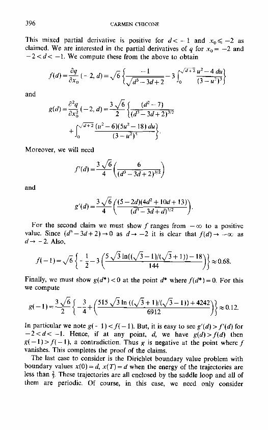
396 CARMEN CHICONE

This mixed partial derivative is positive for d < - 1 and Xo~<-2 as claimed. We are interested in the partial derivatives of q for Xo = - 2 and - 2 < d< -1. We compute these from the above to obtain

and

Oq { - 3 ~ a'/yVS u2-4 du~ f ( d ) = ~ ( - 2, d) = x/'6 - 1 x / d 3 - 3 d + 2 -o (3 ---u-~J

g(d)=~xqso(-2, d)=3-~26{(d3(d2-7) - 3d+ 2) 3/2

+ f Y (ua-6)(5u2-]-3 --- u ~ 18) du} .

Moreover, we will need

f'(d)=3~46((d3-63d+ 2) 3/2 )

and

g , ( d ) = 3 ~ 4 6 ( ( 5 - 2 d ) ( 4 d 2 + 10d+ 13)) \

For the second claim we must show f ranges from - ~ to a positive value. Since ( d 3 - 3 d + 2 ) ~ 0 as d - ~ - 2 it is clear that f(d)~-oo as d--* -2 . Also,

1 )} _ 5 _ 3 5 )/(x/~+ ) ) - 1 8 ~0.68.

144

Finally, we must show g(d*)<0 at the point d* where f (d* )=0 . For this we compute

g ' - l ) = ~ - { 3 ( 5 1 5 x / ~ l n ( ( x / ~ + l ) / ( x / ~ - l ) ) + 4 2 4 2 ) } " ~ 0 " 1 2 " - 4 + 6912

In particular we note g( - 1 ) < f ( - 1 ). But, it is easy to see g'(d) > f ' (d) for - 2 < d < - 1 . Hence, if at any point, d, we have g(d)>f(d) then g ( - 1 ) > f ( - 1 ) , a contradiction. Thus g is negative at the point where f vanishes. This completes the proof of the claims.

The last case to consider is the Dirichlet boundary value problem with boundary values x(O)= d, x(T)= d when the energy of the trajectories are less than 2. These trajectories are all enclosed by the saddle loop and all of them are periodic. Of course, in this case, we need only consider


- 2 < d < 1. Since the phase trajectories are all periodic, a nonstandard Dirichlet situation, there are many different possible solutions for the boundary value problem. To see this consider a fixed d in the interval - 2 < d < 1. Given T we seek, as usual, a trajectory which starts at a point on the line x = d and returns to the line after transit time T. However, unlike the cases already considered the trajectory can lie entirely to the left of x = d, entirely to the right of x --- d, or the trajectory could start on x = d, traverse a periodic orbit a number of times, then return to the line x = d. It is not clear how to formulate a general proposition which covers every case. We are content to establish three properties: (1) The Dirichlet boundary value problem with boundary values x ( 0 ) = d , x ( T ) = d has a nontrivial solution (with energy less than 2) for - l < d < l and for - 2 < d ~ < - 1 has a nontrivial solution t'or T sufficiently large, ( 2 ) f o r - 2 < d < 1 and any integer N there exists a T for which there ai'e at least N solutions, and (3) for fixed D and fixed T there are at most a finite number of solutions.

The first proposition follows by considering only trajectories which lie entirely to the right of x = d and observing that as E ~ ~ the transit time increases to infinity as the trajectories approach the saddle point while for d > 1 the smallest transit time for such a trajectory is zero. The second proposition follows from essentially the same observation. Just consider the minimum period M of the periodic orbits which intersect x = d and choose T = NM. Then T/k >1 M for k = 1, 2 ..... N. But, since the periods of the trajectories intersecting x = d range to infinity there is a periodic trajectory with period T/k which when traversed k times corresponds to a solution of the Dirichlet boundary value problem. Finally, to see there are only a finite number of solutions for fixed d and T consider the possibilities. The phase trajectory which represents the solution could contain k circuits of a periodic trajectory with k < T/(~/2 n), and then at most one "half ' circuit of a periodic trajectory, i.e., a portion of a periodic trajectory which lies in one of the half planes determined by the line x = d. Consider the graphs y = q,,(E) = nP(E), where n = 0 ..... k and P is the minimum period of the periodic trajectory with energy E, - ~ < E<-~ and the graphs y = qr(E), y = qz(E) representing the transit times of the "half ' periods to the right and to the left of the line x = d. A solution for the Dirichlet problem must correspond to a transit time of the form y=qn(E)+qr (E) or y = q,,(E)+qz(E) for some integer n, O<~n<~k. But, since each function represented as such a sum is analytic on --~ ~< E < ~, there is a removable singularity at E = -~-, it is clear that each of these functions has a graph which meets the line y = T at most a finite number of times. In fact, if a summand is either q, , n > 0 , or qr then the sum ranges to + ~ . The function qz can decrease as E ~-~, but it has at most a finite number of critical points.

398 CARMEN CHICONE

For the example of Fig. 4, we have 5 ~ = ¼ ( x + 5 ) ( x - 1 ) so the dis- criminant is positive and 0 = D > - 1. It follows from the first part of our proof of Case 3 that there are exactly two solutions.

There are of course, as mentioned in the Introduction, hypotheses different from those we are working with which also lead to interesting results. One such set of hypotheses is F ( - s ) = F ( s ) , F ( s ) < 0 for s # 0 , G(L) = 0 for some L < 0, and G'(s)> 0 for t >~ L. Under these assumptions the Dirichlet boundary value problem

Yc = F(Yc) + G(x)

x(O) = O, x (T) = 0

always has a solution. To see this look in the phase plane and note that for [Yl large the vector field in the strip {(x, y): L ~< x ~<0} points toward the x-axis. Thus, the unstable separatrix leaving the saddle point at (L, 0) must cross the positive y-axis. By symmetry the stable separatrix in the lower half plane meets the negative y-axis and our usual continuity argument implies there is some a < 0 lying above the stable sepratrix so that the trajectory starting at (0, a) arrives at the negative x-axis in exactly time T/2.

EXAMPLE. Consider the singular perturbation problem [7, p. 144]

p>~2

A > 0 .

Problems of this type can cause some difficulty because solutions of the reduced equation x - [ k [ p = 0 are not unique. From our point of view to study the question of existence of solutions for e > 0 we do not consider the problem as a singular perturbation but as a Dirichlet boundary value problem. If we fix e > 0 and p >/2 and consider the change of variables u = x - A we are led to study the existence of solutions for the Dirichlet problem

/~_-1 ( u + A ) - I I~lp

u (0 )=0 , u ( 1 ) = 0

which satisfies the hypotheses just mentioned above with F(s)= - 1/elsL p and G(s)= 1/e(u + A). Hence there is a solution for each e > 0.

We now begin the main portion of this section where we explore how the existence of solutions for the Dirichlet boundary value problem is affected

e ~ = x - ] ~ ] P ,

x(0, ~) = A

x(1, e) = A,


by the growth rate of F. To illustrate this relationship consider 5~ = F(.¢c) + G(x) where F and G satisfy the hypotheses of this section. In addition assume G has no negative zero and G ( x ) ~ G ( - o o ) > O as x ~ -oo . We have just seen in the proof of Corollary 3.3 that there is only one possibility for which the boundary value problem has no solution. This could occur only i fp(a) is defined for all a ~ ( - 0% 0] and

f T 0 d y ' ~ - - .

,~ G ( x ( y , ~ ) ) + F ( y ) 2

Since

fo dy [o dy -oo G(x) + F ( y ) < ~ G( - oo ) + F ( y )

there will be no solution if

f o dy T

-oo G ( - o o ) + F ( y ) 2

If the growth rate of F is faster than some power function, i.e., F(y)>~ aly] p for a > 0, p ~> 1, then

f f° o dy <

-oo G ( - o o ) + F ( y ) _ ~ G ( - o v ) + a l y l p

G( - oo ) p sin n/p"

(The integral can be computed using a contour integration in the complex plane.) Therefore, there is no solution if

G ( - o o ) p s i n n / p 2

The left hand side of the inequality tends to oo as p---} 1 and to ( G ( - o o ) ) 1 as p ~ oo. Thus for large p solutions are less likely. Also, for fixed p > 1, there is always some choice for a for which no solution exists.

EXAMPLE. Consider the boundary value problem

5~= 1 + eX + al~l p

x(O)=O, x(1)=0.

505/72/2-14

400 CARMEN CHICONE

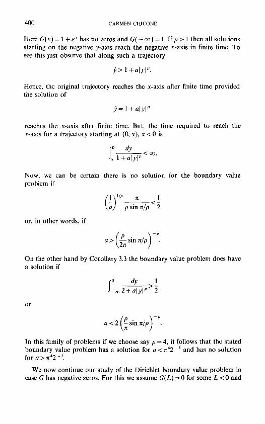
Here G(x) = 1 + e x has no zeros and G( - oo ) = 1. If p > 1 then all solutions starting on the negative y-axis reach the negative x-axis in finite time. To see this just observe that along such a trajectory

p> 1 +alyl p.

Hence, the original trajectory reaches the x-axis after finite time provided the solution of

p= 1 + al yl p

reaches the x-axis after finite time. But, the time required to reach the x-axis for a trajectory starting at (0, ~), ~ < 0 is

i~ dy <c~. l + a ] y l p

Now, we can be certain there is no solution for the boundary value problem if

p sin n/--------p <

or, in other words, if

On the other hand by Corollary 3.3 the boundary value problem does have a solution if

f o dy 1 _.~ 2 + a l y l P > 2

o r

a < 2 (Psin n/p) -p.

In this family of problems if we choose say p = 4, it follows that the stated boundary value problem has a solution for a < n42 5 and has no solution for a > n42-2.

We now continue our study of the Dirichlet boundary value problem in case G has negative zeros. For this we assume G(L) --- 0 for some L < 0 and


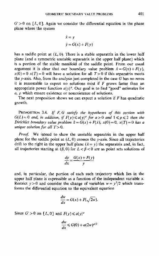
G ' > 0 on [L, 0]. Again we consider the differential equation in the phase plane where the system

~ = y

y = G(x) + F(y)

has a saddle point at (L, 0). There is a stable separatrix in the lower half plane (and a symmetric unstable separatrix in the upper half plane) which is a portion of the stable manifold of the saddle point. From our usual argument it is clear that our boundary value problem 5~=G(x)+F(y) , x(O) = 0 x ( T ) = 0 will have a solution for all T > 0 if this separatrix meets the y-axis. Also, from the analysis just completed in the case G has no zeros it is reasonable to expect no solutions exist if F grows faster than an appropriate power function aiyl p. Our goal is to find "good" estimates for a, p which ensure existence or nonexistence of solutions.

The next proposition shows we can expect a solution if F has quadratic growth.

PROPOSITION 3.4. I f F, G satisfy the hypotheses of this section with G(L) = 0 and, in addition, i f F(y) <~ alYl p for a > 0 and 1 <~ p <~ 2 then the Dirichlet boundary value problem 5~ = G(x) + F(£¢), x(O) = O, x(T) = 0 has a unique solution for all T> O.

Proof We intend to show the unstable separatrix in the upper half plane for the saddle point at (L, 0) crosses the y-axis. Since all trajectories drift to the fight in the upper half plane (~ = y) the separatrix and, in fact, all trajectories starting at (fl, 0) for L < fl < 0 are as point sets solutions of

dy G(x) + F(y)

dx y

and, in particular, the portion of each such trajectory which lies in the upper half plane is expressible as a function of the independent variable x. Restrict y > 0 and consider the change of variables w = y2/2 which transforms the differential equation to the equivalent equation

d w i------ = G(x) + F(x/2w).

Since G ' > 0 on [L, 0] and F(y)<~alYl p

dw ~xx ~< G(0) + a(2wF/z

402 CARMEN CHICONE

so any trajectory of the original differential equation starting at remains bounded by the corresponding trajectory of

dw dx G(0)+a(2w) "/2.

(/~, o)

But, the trajectory of this equation satisfies

i:,(x) dz G(O) + a(2z) p/2 = Xo - ft.

This trajectory either is unbounded as x--* Xo, fl < Xo ~< 0 in which case

fo o dz G(O) + a(2z ) p/2 = Xo - fl < oo

or the trajectory meets the y-axis in which case

W(° dz G(O) + a(2z) p/2 = - fl < oo.

Thus, if

~o ~ G(O) + a(2z) p/2 = ~

the second alternative must obtain. But, this is the case when p ~< 2. The uniqueness follows from Proposition 3.1. |

To obtain estimates for the nonexistence of solutions we keep our usual hypotheses on F and G but we now assume F(y)>~aly[ p, a > 0 and p > 2. In light of the proof just completed it is easy to form a strategy to show the nonexistence of solutions. First, we must have the stable separatrix of the saddle point at (L, 0) not intersecting the y-axis. Next we find a trajectory which starts at (fl, 0) for some f l • (L, 0) which also does not meet the y-axis. Clearly, a trajectory starting at (0, 0t), ~t < 0 on the y-axis stays to the right of this barrier trajectory. In particular, in the presence of a barrier trajectory any trajectory starting at (0, ~) meets the x-axis in finite time at some point in the interval (fl, 0). Finally, there will be no solution if p(ot) < T /2 for all ~ • ( - ~ , 0].

Suppose for the moment the trajectory through (fl, O) is a barrier trajectory and consider the trajectory starting at (0, ~), ~ > O. We know

o dy f p ( a ) J, a(x(y, ~)) + F(y)"


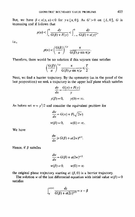
But, we have fl < x(y, ~) < 0 increasing and if follows that

f0 dy p(~) < J~ G(fl) + F(y)

i.e.,

for y ~ [ ~ , 0 ] . As G'>0 on

fo dy

< - ~ G(f l )+alYl" '

P(~) < G(fl) p sin rc/p"

[L, 0], G is

Therefore, there would be no solution if this sojourn time satisfies

G(fl) p sin n/p

Next, we find a barrier trajectory. By the symmetry (as in the proof of the last proposition) we seek a trajectory in the upper half plane which satisfies

dy G(x) + F(y) dx y

y(fl) = O, y(O) = ~ .

As before set w = y2/2 and consider the equivalent problem for

dw --~x = G(xl + F( ,~ /~)

We have

w@=0, w(0)=~.

dw >t G(fl) + a(2w) p/z.

Hence, if fl satisfies

dw = G(fl) + a(2w) "/2

w ( # ) = O, w(O) =

the original phase trajectory starting at (fl, 0) is a barrier trajectory. The solution w of the last differential equation with initial value w(fl) = 0

satisfies

dZ ~__Xm~ Io t'~ G(fl) + a(2z) p/2

404 CARMEN CHICONE

and a solution satisfying w(0) = ~ exists if and only if

~o ~ dz G(fl) + a(2z) p/z = - fl,

i.e.,

G(3) p sin 27t/p - ~"

Hence, by our comparison, the trajectory starting at (/~, 0) for the original equation will be a barrier trajectory if

a ( ~ ) 0 sin 2~ /0 ~< - ~"

Now, a proposition on nonexistence follows easily.

PROPOSITION 3.5. I f F, G satisfy the hypotheses o f this section with G(L) = 0 and F(y) >~ a]yl p, p > 2, then there is some value o f a > 0 for which the Dirichlet boundary problem 5~ = F(J¢) + G(x), x(O) = O, x (T ) = 0 has no solution.

Proof Fix p > 2 and any fie (L, 0) we must show there is some a > 0 for which

G(/~) p sin n/p

and

G([3) p sin 2n/p <<" - [3.

But, it is clear the left hand side of each inequality tends to zero as a ---~ oo. |

In view of the last proposition we know solutions for our boundary value problems do not exist for large values of a. If we fix T, L, and p > 2, we would like to find a number A > 0 such that a > A implies there is no solution. Using the two sufficient conditions determined above an easy calculation shows A is such a bound if A satisfies both

A >>. { T p \ 2~ ]P 1 sin rc/p l " G ( ~ " -


and

1

A >~ P sin 2n/pJ (--#)p/2G(fl)(P-2)/2

for some fl s (L, 0). By considering the graphs of the two functions of fl on the right hand sides of the inequalities and by taking into account the growth rates as f l ~ L +, in short that p - 1 > ( p - 2 ) / 2 , it is easy to see there is one point B where the right hand sides are equal and that this choice of fl determines the smallest value of A which satisfies both inequalities.

In the above generality we cannot solve for B explicitly. However, we compute

G(B) 4n sin 2n/p - B = T2p sin E n/p

from which fl can be estimated in examples.

EXAMPLE. Consider the Dirichlet boundary value problem £ = 1 +x+aJ£Jp ; x ( 0 ) = 0 , x ( 1 ) = 0 . Here G ( x ) = 1 + x , so L = - 1 . We compute

- p sin E n/p B =

p sin E nip + 4n sin 21r/p

and then

2n ]P(.psin2n/p+4nsin2n/p) p-I A = p sin n/pl \ 4n sin 2n/p

To be even more specific if we take p = 4 we obtain

A = n(2n + 1)3 ~ 38. 25

This should be compared with the bound

38 A = ~ 2 0 5

obtained in [13, p. 43]. Also, from our Corollary 3.3 we find that there is a unique solution for the boundary value problem when

f o dz 1

> 5

406 CARMEN CHICONE

or when

a < ~24.

Thus, the bifurcation value lies in the interval (24, 38). Some computer experiments suggest the bifurcation value actually falls in the interval (32, 33).

ACKNOWLEDGMENTS

I thank the Brazilian National Science Council (CNPq) for supporting me during the summer of 1985 at IMPA in Rio de Janeiro where this work was begun. I especially thank Jorge Sotomayor for his hospitality at IMPA and for many helpful conversations which contributed to the completion of this paper.

REFERENCES

1. V. I. ARNOLD, "Geometric Methods in the Theory of Ordinary Differential Equations," Springer-Verlag, New York/Berlin, 1983.

2. P. BAILEY, L. SHAMPINE, AND P. WALTMAN, Nonlinear two point boundary value problems, in "Mathematics in Science and Engineering," Vol. 44, Academic Press, 1968.

3. R. BERNFELD AND V. LAKSHMIKANTHAM, "An Introduction to Nonlinear Boundary Value Problems," Academic Press, New York, 1974.

4. S. N. BERNSTEIN, Sur les 6quations du calcul des variations, Ann. Sci. l~cole Norm. Sup. 29 (1912), 431-485.

5. R. I. BOGDANOV, Bifurcation of limit cycles of a family of plane vector fields, Selecta Math. Soviet 1 (1981), 373-387.

6. J. CARR, S. N. CHOW, AND J. K. HALE, Abehan integrals and bifurcation theory, J. Dif- ferential Equations, to appear.

7. K. W. CHANG AND F. A. HOWES, Nonlinear singular perturbation phenomena: Theory and application, in "Applied Mathematical Sciences," No. 56, Springer-Verlag, New York/Berlin, 1984.

8. C. CH1CONE, The monotonicity of the period function for planar Hamiltonian vector fields, preprint, 1986.

9. S. N. CHOW AND J. K. HALE, "Methods of Bifurcation Theory," Springer-Verlag, New York/Berlin, 1982.

10. S. N. CHOW AND J. A. SANDERS, On the number of critical points of the period, to appear. l 1. S. N. CHOW AND D. WANG, On the monotonicity of the period function of some second

order equations, to appear. 12. R. H. CUSHMAN AND J. A. SANDERS, A codimension two bifurcation with a third order

Picard-Fuchs equation, Differential Equations 59 (1985), 243-256. 13. A. GRANAS, R. B. GUENTHER, AND J. W. LEE, Nonlinear boundary value problems for

some classes of ordinary differential equations, Rocky Mountain J. Math. 10 (1980), 35-58.

14. A. GRANAS, R. B. GUENTrmR, AND J. W. LEE, Topological transversality. II. Applications to the Neumann problem for y" =f(t , y, y'), Pacific J. Math. 104 (1983), 95-109.


15. S. B. Hsu, A remark on the period of the periodic solution in the Lotka-Volterra systems, J. Math. Anal AppL 95 (1983), 428-436.

16. J. M. LASRY AND P. L. LIONS, Equations elliptiques non lin6aires avec conditions aux limites infinies et contr61e stochastique avec contraintes d'6tat, C. R. Acad. St'. Pans Skr. I 299 (7) (1984), 213-216.

17. W. S. Lout), Periodic solution of x" + cs' + g( x ) = ef ( t ), Mere. Amer. Math. Soc 31 (1959), 1-57.

18. C. O~1, Analytical theory of nonlinear oscillation. VII. The periods of the periodic solutions of the equation x " + g(x)=0 , J. Math. Anal, Appl. 55 (1976), 295-301.

19. Z. OP1AL, Sur les p6riodes des solutions de l'~quation diff~rentielle x " + g (x )= O, Ann. Polon. Math. 10 (1961), 49-72.

20. F. ROXWE, Thermodynamics, real and complex periods of the Volterra model, J. Appl. Math. Phys. 36 (1985), 395-421.

21. F. Roxrn~, Periods of oscillation, nondegeneracy and specific heat of Hamiltonian systems in the plane, to appear in "Proceedings of the International Conference on Differential Equations and Mathematical Physics, Birmingham, Alabama, 1986."

22. R. SCHAAF, A class of Hamiltonian systems with increasing periods, J. Reine Angew. Math. 363 (1985), 96-109.

23. R. SCHAAF, Global behaviour of solution branches for some Neumann problems depending on one or several parameters, J. Reine Angew. Math. 346 (1984), 1-31.

24. J. S~4OLLER AND A. WASSEa~IAN, Global bifurcation of steady-state solutions, J. Differen- tial Equations 39 (1981), 269 290.

25. D. WANG, On the existence of 2~-periodic solutions of differential equation x " + g (x )= p(t), Chinese Ann. Math. Set. A 5(1) (1984), 61-72.

26. J. WALDVOGEL, The period in the Lotka-Volterra predator-prey model, S l A M J. Numer. Anal. 20 (1983).

27. J. WALDVOGEL, The period m the Lotka-Volterra system is monotonic, preprint. 28. V. LUNKEVlCH AND K. SIBIRSKII, Integrals of a general quadratic differential system in

cases of a center, Dtfferentlal Equations 18 (1982), 563-568.

Geometric Methods for Two-Point Nonlinear Boundary Value ... · Geometric Methods for Two-Point Nonlinear Boundary Value Problems CARMEN CHICONE* ... 0 is always a solution. We are

Documents