Gas-water Contacts, Free Water Levels Analysis in Support ... · Irene Platteeuw and Akira Toriyama. And finally, I would like to acknowledge my parents and my sister for their continued

Gas-Water Contacts, Free

Water Levels analysis in

support of petroleum

exploration in offshore

Netherlands

Belabed, Malik

2

3

Gas-Water Contacts, Free Water Levels analysis

in support of petroleum exploration in offshore

Netherlands

By

Belabed, Malik

4129989

in partial fulfilment of the requirements for the degree of

Master of Science

in Applied Earth Sciences, specialization Petroleum Engineering

at the Delft University of Technology,

to be defended publicly on Tuesday August 29, 2017 at 10:30 AM.

Supervisor: Dr. K.H.A.A. Wolf, T.U. Delft Thesis committee: Drs. J.E. Lutgert, EBN B.V.

Dr. A. Barnhoorn, T.U. Delft Prof. Dr. W.R. Rossen, T.U. Delft Dr. M.H.H. Hettema EBN B.V.

This thesis is confidential and cannot be made public until September 1, 2017.

4

An electronic version of this thesis is available at http://repository.tudelft.nl/.

5

Abstract

Hydrocarbon (HC) contact depths, e.g. gas-water contacts (GWCs) in a HC reservoir are crucial for

volumetric and petrophysical calculations. It is therefore of great importance to determine the GWC and

free water level (FWL) correctly and to understand the uncertainties and (often financial) limitations

these determinations inherently possess.

The aim of this study was to enhance the subsurface knowledge of the K- and L- blocks of offshore

Netherlands through an analysis of HC contact depths using operator data, log evaluation, pressure data

and saturation modelling. The goal was also to ultimately assess the significance of HC contact depth

and uncertainty in support of petroleum exploration, and to provide innovative new ways to asses

reservoir characteristics using HC contact depths.

Using data from approximately 122 wells, the K- & L-blocks of offshore Netherlands have been mapped

using operator-sourced data, and verified using pressure data, quick-look petrophysical analysis and

saturation modelling. The Permian basins form the overwhelming majority of data with 81% being

Upper or Lower Slochteren Member. An uncertainty analysis of the Slochteren Formation shows that

the pore throat radius is the most important variable for the capillary height. The capillary height is

defined by the difference in depth between the GWC and FWL. The operator standard deviation in

FWL/GWC height is approximately 55 m for the Slochteren Formation.

Using data visualisations, it can be concluded that the age of the formation containing the HC contact

increases going westwards. Triassic gas-filled reservoirs are solely present in the easternmost region of

the L-block, whereas the oldest gas-filled Carboniferous reservoirs are present in the northwestern part

of the K-block. The Slochteren Formation also displays a clear separation, with the Upper Slochteren

gas-fill being situated more in the southeastern part and the Lower Slochteren towards the northwestern

part of the region.

The HC contact database can be used to validate the compaction of reservoir materials judging by the

change in the capillary height, and the facies distribution of the Upper Slochteren can be verified using

the HC contact database. Assuming that the other variables in the capillary equation remain constant,

we can see that the pore throat radius reduces with approximately 28.8% in the fluvially dominated part

of the Upper Slochteren sandstone.

6

Acknowledgements

Firstly, I would like to express my sincere gratitude to dr. Karl-Heinz Wolf, drs. Nora Heijnen and, drs.

Jan Lutgert for their extraordinary support in this thesis process. Their guidance helped me greatly with

my research and writing of this thesis.

I would like to thank drs. Abdul Hamid for always being willing to help me. My sincere thanks also go

to Jurgis Claudius and Lloyds Register for providing me software ( Interactive Petrophysics) which has

greatly aided me during my research.

I also would like to thank my fellow EBN students Jan Westerweel and Mathijs Kuiper for their help

with TIBCO Spotfire. Special mentions go to Daniel Aramburo, Constantijn Blom, Eelco Mechelse,

Irene Platteeuw and Akira Toriyama.

And finally, I would like to acknowledge my parents and my sister for their continued support during

my entire life.

Belabed, Malik

Delft, August 2017

7

Contents

Abstract ................................................................................................................................................................... 4

Acknowledgements ................................................................................................................................................. 6

List of Figures ........................................................................................................................................................... 8

List of Tables ............................................................................................................................................................ 8

Symbols and Subscripts ........................................................................................................................................... 9

Abbreviations ......................................................................................................................................................... 10

Introduction ........................................................................................................................................................... 11

Research Questions ........................................................................................................................................... 13

Definitions of Terms .............................................................................................................................................. 14

Regional Geology ................................................................................................................................................... 19

Upper Rotliegend Group ................................................................................................................................... 20

Ten Boer Member (ROCLT) ............................................................................................................................... 21

Slochteren Member (ROSL) ............................................................................................................................... 21

Ameland Member (ROCLA) ............................................................................................................................... 22

Structural Geology ................................................................................................................................................. 22

Reservoir Characteristics ....................................................................................................................................... 24

Hydrocarbon Contact Database ............................................................................................................................. 26

Methodology ..................................................................................................................................................... 26

Uncertainty Analysis .............................................................................................................................................. 35

Sources of Petrophysical Uncertainty ............................................................................................................... 36

Quantification of Wireline Depth Measurement Uncertainty ........................................................................... 37

Gaussian Error Propagation .......................................................................................................................... 37

Operational Measurement Error .................................................................................................................. 38

Sensitivity Analysis of Capillary Rise .................................................................................................................. 39

Gaussian Error Propagation .......................................................................................................................... 39

Monte Carlo Simulation ................................................................................................................................ 40

Data Visualisations and Discussion ........................................................................................................................ 42

Further Discussion ............................................................................................................................................. 49

Recommendations ................................................................................................................................................. 51

Conclusions ............................................................................................................................................................ 52

Bibliography ........................................................................................................................................................... 53

Appendix ................................................................................................................................................................ 56

Appendix A ........................................................................................................................................................ 56

Appendix B ........................................................................................................................................................ 62

Appendix C ........................................................................................................................................................ 63

8

List of Figures

Figure 1:Overview of reservoirs in the Netherlands [created with TIBCO Spotfire] ............................11 Figure 2: Saturation and capillary pressures in the transitional zone between the gas- and water leg,

after [ Spearing, M., C., et al., 2014] ......................................................................................................14

Figure 3: Schematic overview of the gas-water capillary transition zone, after [Bera, A., Belhadj, H.,

2016] .......................................................................................................................................................15 Figure 4: Cross-sections of oil-wet and mixed-wet porous media [Mohammadi, S., 2015] ..................16 Figure 5: Cap curves ..............................................................................................................................17

Figure 6: K- and L-blocks of offshore Netherlands ..................................................................................19

Figure 7: Facies distribution at onset of Upper Slochteren Formation distribution, after [Geluk, M., C., 2007] .......................................................................................................................................................20

Figure 8: Stratigraphic cross-section of the Rotliegend Group, after [Van Hulten, F., F., N., 2010] .......21

Figure 9: Illustration of K15-FG field displaying structural geology [Van Hulten, F., F., N., 2010] .........23

Figure 10: Data acquisitioning flow ........................................................................................................26

Figure 11: Model of minimum curvature method [Directional Drilling, PGEngineering] .......................27

Figure 12: Composite well log of well K07-10 .........................................................................................28

Figure 13: Pressure data of well K07-10 .................................................................................................29

Figure 14: IP saturation modelling workflow ..........................................................................................30

Figure 15: Porosity-permeability relationship of Slochteren Sandstone formations using multi-well plot in IP ..........................................................................................................................................................33

Figure 16: Saturation height profile function of Well K08-FA-101, modelled in IP .................................34

Figure 17: Interactive Log plot used to calculate the FWL of Well K08-FA-110, modelled in IP ............35

Figure 18: Uncertainty in depth measurements [Hall,M., 2012] ............................................................36

Figure 19: Logging depth mismatch in well L01-04 ................................................................................38

Figure 20: Operator FWL data set of the HC contact database (N= 122) ...............................................42

Figure 21: East-west oriented cross-section of the HC contact data set in the K- and L-blocks of offshore Netherlands ...............................................................................................................................44

Figure 22: Pressure depth plot of the cross-section of Figure 16 ............................................................44

Figure 23: (a) Crude contour map of the operator base FWL data set in the HC contact database, contour interval 100m (b) Detailed contour map of the operator base FWL data set in the HC contact database, contour interval 100m ............................................................................................................45

Figure 24: Overlay of structural element map on the HC contact database [EBN WMS Server]............46

Figure 25: Regional reservoir facies distribution map of the Upper Slochteren Member overlain on the HC contact database, after [ Doornenbal, H., 2010] ...............................................................................47

Figure 26: Reservoir facies distribution map of the Upper Slochteren Member overlain on the HC contact database, after [Doornenbal, H., 2010] .....................................................................................47

Figure 27: FWL difference between the optimistic and pessimistic FWL determination of operators ...48

Figure 28:Crossplots of induction resistivity (ILD) and porosity (%) showing bad-hole effects, (A) sonic, (B) density, (C) neutron, (D) neutron avg., (E) borehole-and-shale corrected effective porosity. [Moore, W., R., 2011] ............................................................................................................................................62

List of Tables

Table 1: Wettability rules of thumb for a two-phase system consisting of water and oil phases [Craig,

F., F., J., 1993] .......................................................................................................................................17

9

Table 2: Summary of typical pore throat size and reservoir parameters for siliciclastic rocks [Nelson, P.,H., 2009] ..............................................................................................................................................25

Table 3: Gas compositions for gas-water IFT range [Rushing, J., A., et al., 2008] ..................................25

Table 4: Wireline depth measurement potential errors [Theys 1991, Sølly and Rodgers 1994] ............37

Table 5: Variable value ranges used for Monte Carlo .............................................................................40

Table 6: Results of sensitivity analysis ....................................................................................................41

Table 7: HC contact Database .................................................................................................................56

Table 8: Monte Carlo Dataset .................................................................................................................63

Symbols and Subscripts

Greek Symbols Subscripts

θ [ °] Contact angle w Wetting Phase

µ [Pa·s] Viscosity nw Non-wetting Phase

ρ [kg·m-3] Density r Residual

σ [N·m-1] Interfacial tension wc Connate water

ϕ [V/V] Porosity c Capillary

γ Specific Gravity g Gas

HC Hydrocarbon

rg Residual Gas

Latin Symbols Other

A [m2] Area ° Degree

G [m·s-2] Gravitational acceleration

K [m2] Permeability

Nc Capillary number

P [Pa] Darcy-scale pressure

p [Pa] Pore-scale pressure

Q [m3·s-1] Volumetric flow rate

S Saturation

t [s] Time

u [m s-1] Velocity

V [m3] Volume

x [m] Distance from well

10

Abbreviations

ARPR Annual Review of Petroleum Resources

BVW Bulk Volume Water Log

CSP Clay Smear Potential

FWL Free Water Level

GIIP Gas Initially In Place

GR Gamma-ray Log

GWC Gas-Water Contact

HC Hydrocarbon

IFT Interfacial Tension

ILD Induction Resistivity

NT Neutron Log

OWC Oil-Water Contact

PHI Porosity Log

REV Representative Elementary Volume

RFT Repeat Formation Test

RMA Reduced Major Axis

RT Resistivity

SGR Shale Gouge Ratio

SSF Shale Smear Factor

ST Sonic Log

TVD(SS) True Vertical Depth (Subsea)

DC Limburg Group

RBMVL Lower Volpriehausen Member

RNSO Sollingen Member

ROCLA Ameland Member

ROCLE Silverpit Evaporite Member

ROCLL Lower Silverpit Claystone Member

ROCLT Ten Boer Member

ROSL Slochteren Formation

ROSLL Lower Slochteren Member

ROSLU Upper Slochteren Member

11

Introduction

Much of the gas production–related infrastructure in offshore Netherlands is aging. The concern is that

significant amounts of gas may be left behind when gas fields and production facilities are abandoned

[Van Hulten, F., F., N., 2010]. Fluid-contact depths are vital in the calculation of field reserves and for

field development [Thulin, K., et al., 2007]. Besides being used for reservoir characterisation and

volumetric calculations, fluid-contact depths can also be used to analyse regional trends in an area where

a large number of reservoirs exist, i.e. a petroleum play. The Permian Basin in the Southern North Sea

is such a petroleum play. It is an area which has been of continuing interest for the past 55 years, since

the discovery of the Groningen Gas Field [Moscariello, A., 2014]. The Southern Permian Basin—and,

in particular, the Rotliegend Group—is critically important, as approximately 95% of Dutch natural gas

reserves are situated in Permian reservoirs [Geluk, 2007], with more than 50% of these gas fields

producing from the Rotliegend [Van Hulten, F., F., N., 2010]. These fields are located in an east-west

corridor called the Rotliegend fairway [Van Wijhe et al., 1980; Glennie 1998; Wong et al., 2007].

Triassic Bunter, Permian Zechstein, Upper Carboniferous, Cretacious and Tertiary formations are less

numerous [Van Hulten, F., F., N., 2010]. Figure 1 displays a geographic map of all of the HC reservoirs

in the subsurface of the Netherlands and surrounding countries, the focus of this research—which are

the K-&L- blocks of offshore Netherlands,—has been highlighted in yellow.

Figure 1:Overview of reservoirs in the Netherlands [created with TIBCO Spotfire]

12

In this report, a detailed methodology for the creation of a HC contact database is stipulated. The HC

contacts of approximately 122 fields are analysed and documented. For 73 fields the column height has

been calculated. The strengths and limitations of the database are discussed, and an analysis of the

contacts is given along with multiple innovative ways in which these results can be used.

Recommendations are given for future studies, and possibilities for expanding and enhancing the

database are discussed.

The aim of this study was to enhance the subsurface knowledge of reservoir spill points through an

analysis of HC contact depths using log evaluation and pressure data.

Specifically, using log and pressure data from several operators (e.g. NAM, Total, Engie), a HC contact

database was constructed with a focus on the K- and L-blocks of offshore Netherlands. The uncertainties

and/or discrepancies of these contacts were thoroughly analysed through the use of an uncertainty

analysis. The methodology involved using the HC contact database to chart the reservoir gas-water

contact (GWC)/ free water levels (FWLs), thus enabling an analysis of reservoir properties relevant to

capillary rise. By using the existing knowledge of the regional geology, the HC database is used to

visualize the region with respect to e.g. reservoir compaction and facies distribution. In this way, the

research aims to support petroleum prospectivity in the K- and L-blocks of offshore Netherlands.

This study can be used to enhance the knowledge of the HC contact depths in the subsurface in offshore

Netherlands. It can serve as a guide for how to perform a HC contact analysis. This study is a first, as a

complete analysis of the K- and L- blocks has not been conducted because several operators cover the

area. As such, this study can shed light on the regional spill point behaviour through the use of

GWC/FWL trends. Furthermore, under the section Data Visualisations and Discussion, innovative

examples are provided of how information in the HC contact database can be used to determine, and

validate, reservoir characteristics such as compaction and facies distributions.

The HC contact height is critical in net pay determination and, by extension, for volumetrics. The goal

of net pay calculations is to eliminate non-productive rock intervals and, from these calculations at the

various wellbores, to provide a solid basis for a quality three-dimensional reservoir description and

quantitative HC-in-place calculation. This is primarily done by determining various cut-off criteria but

also by considering the height of the gas column in the reservoir. As such, errors in the contact height

reflects back in net pay calculations. By varying the height of the GWC/FWL, a reservoir can be deemed

economically viable and given the go-ahead for production, or vice versa. This means that an error in

the determination of the GWC/FWL can have very grave (financial) implications for an operator. In a

13

worst-case scenario, a reservoir can end up not being economically viable and a total write-off for the

operator. As such, a thorough petrophysical evaluation of a reservoir is imperative.

Research Questions

What are the strengths and weaknesses of the HC contact database?

How can the HC contact database aid in inferring the presence of new prospects in the K- & L-

blocks of offshore Netherlands?

How can a quantitative approach to dealing with uncertainties in HC contact measurements be

derived?

How do the uncertainties of different HC measurements, i.e. pressure or log data compared, add

up to a global error?

How can the HC contact data be used to characterise reservoir properties?

What are the HC contact trends in the K- & L-blocks of offshore Netherlands, and what are the

correlations behind these trends?

14

Definitions of Terms

Before we can proceed with a more detailed examination of the various reservoir characteristics and the

various processes which can influence HC contact height, some definitions may be helpful. Most of

these definitions were obtained from extracts of a technical paper by T.R. Pham et al. [Pham, T., R.,

2015] and were modified to suit this research. The main difference is that Pham analysed three phase

systems, whereas we focus solely on a two-phase system consisting of a gas and water phase.

Residual gas saturation (Srg) is the minimum gas saturation required in a system for the gas to be mobile.

Likewise, connate (or irreducible) water saturation (Swc) is the water saturation under which no

movement of the water phase is possible in a system.

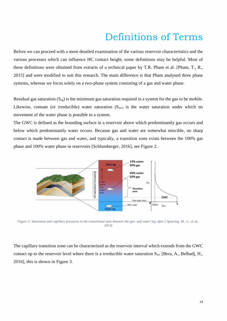
The GWC is defined as the bounding surface in a reservoir above which predominantly gas occurs and

below which predominantly water occurs. Because gas and water are somewhat miscible, no sharp

contact is made between gas and water, and typically, a transition zone exists between the 100% gas

phase and 100% water phase in reservoirs [Schlumberger, 2016], see Figure 2.

Figure 2: Saturation and capillary pressures in the transitional zone between the gas- and water leg, after [ Spearing, M., C., et al.,

2014]

The capillary transition zone can be characterized as the reservoir interval which extends from the GWC

contact up to the reservoir level where there is a irreducible water saturation Swc [Bera, A., Belhadj, H.,

2016], this is shown in Figure 3.

15

Figure 3: Schematic overview of the gas-water capillary transition zone, after [Bera, A., Belhadj, H., 2016]

The FWL in a reservoir is the level at which no wetting/non-wetting phase capillary pressure exists. It

is the theoretical interface which would exist in equilibrium in an observation borehole, without capillary

effects, if it were to be drilled through a two-phase system.

As can be seen in Figure 3, the capillary rise is defined by the height difference between the FWL and

the GWC. See eq. (19) for the governing equation of capillary rise. It is a modified capillary pressure

equation. Capillary pressure (Pc) is defined as the excess pressure of the non-wetting phase. It can be

defined by the following:

𝑃𝑐 = 𝑃𝑛𝑤 − 𝑃𝑤 (1)

Capillary pressure is (among others) dependent on the saturation of each phase, on the wetting behaviour

of the reservoir and on the size and distributions of the pores and pore throats.

The displacement pressure (Pd) is the minimal capillary pressure which is required for the non-wetting

phase to surpass the largest pore throat radius and displace the wetting phase.

Drainage is defined as the process which occurs when the non-wetting phase displaces the wetting phase,

thus increasing the non-wetting phase’s saturation. Imbibition is the exact opposite of drainage. With

imbibition, the wetting phase’s saturation increases, and the non-wetting phase decreases.

When water is in the process of invading a gas reservoir, the gas formation pressure Pf will be altered.

The invading water will cause the reservoir pressure to rise. If in such a case the reservoir pressure is

sampled, pressure Ps will be measured. The difference between Pf and Ps (which δP characterises) is

16

known as supercharging in tight formations. This δP is the existing capillary pressure. In this research,

the supercharged points of measurement are not used. Instead, solely valid measurement points are used

in further analysis.

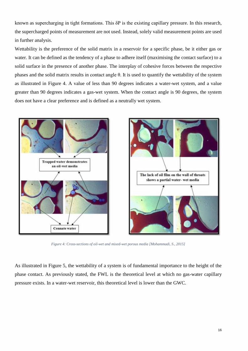
Wettability is the preference of the solid matrix in a reservoir for a specific phase, be it either gas or

water. It can be defined as the tendency of a phase to adhere itself (maximising the contact surface) to a

solid surface in the presence of another phase. The interplay of cohesive forces between the respective

phases and the solid matrix results in contact angle θ. It is used to quantify the wettability of the system

as illustrated in Figure 4. A value of less than 90 degrees indicates a water-wet system, and a value

greater than 90 degrees indicates a gas-wet system. When the contact angle is 90 degrees, the system

does not have a clear preference and is defined as a neutrally wet system.

Figure 4: Cross-sections of oil-wet and mixed-wet porous media [Mohammadi, S., 2015]

As illustrated in Figure 5, the wettability of a system is of fundamental importance to the height of the

phase contact. As previously stated, the FWL is the theoretical level at which no gas-water capillary

pressure exists. In a water-wet reservoir, this theoretical level is lower than the GWC.

17

Figure 5: Cap curves

Wettability is an important reservoir parameter. However, no industry (or academic) standard exists

regarding which criteria characterise reservoir wettability. Craig specified the following rules of thumb

which can indicate reservoir wetting behaviour [Craig, F., F., J., 1993]:

Table 1: Wettability rules of thumb for a two-phase system consisting of water and oil phases [Craig, F., F., J., 1993]

Water-Wet Oil-Wet

Connate water saturation Usually greater than

20 to 25% pore

volume

Generally less than 15% pore

volume, frequently less than 10%

Saturation at which oil and water

relative permeabilities are equal

Greater than 50%

water saturation

Less than 50% water saturation

Relative permeability to water at

maximum water saturation, i.e. flood

out

Generally less than

30%

Greater than 50% and approaching

100%

18

Unfortunately, such criteria do not exist for gas reservoirs, and the industry generally assumes gas as a

non-wetting phase [Zhang, M., et al., 2016]. Hagoort indicated that in the case of gas-water systems,

virtually all reservoir rocks are water wet [Hagoort, J., 1988]. This implies that when a gas-saturated

sample is immersed in water, water will largely displace the gas due to imbibition. This assumption,

however, is not always valid. The work of Min Zhang [Zhang, M., et al., 2016] showed that gas wetness

cannot always be overlooked, and the gas-wet degree affects gas well production greatly in gas

condensate reservoirs. Condensate blockage near a wellbore decreases gas productivity. However, this

is not a concern in this research, as virtually all reservoirs in the Dutch subsurface are gas reservoirs, not

gas condensate reservoirs [Van Hulten, F., F., N., 2010].

19

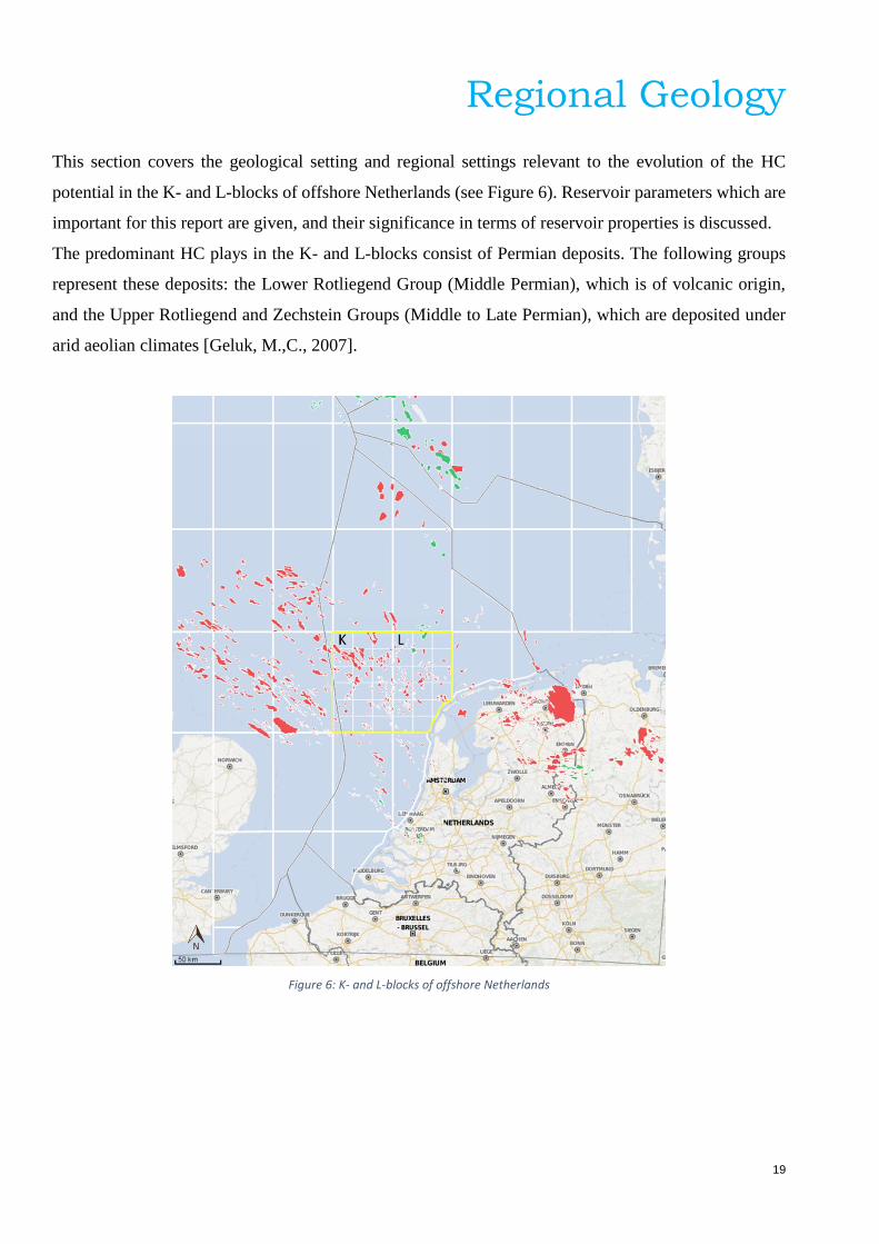
Regional Geology

This section covers the geological setting and regional settings relevant to the evolution of the HC

potential in the K- and L-blocks of offshore Netherlands (see Figure 6). Reservoir parameters which are

important for this report are given, and their significance in terms of reservoir properties is discussed.

The predominant HC plays in the K- and L-blocks consist of Permian deposits. The following groups

represent these deposits: the Lower Rotliegend Group (Middle Permian), which is of volcanic origin,

and the Upper Rotliegend and Zechstein Groups (Middle to Late Permian), which are deposited under

arid aeolian climates [Geluk, M.,C., 2007].

Figure 6: K- and L-blocks of offshore Netherlands

20

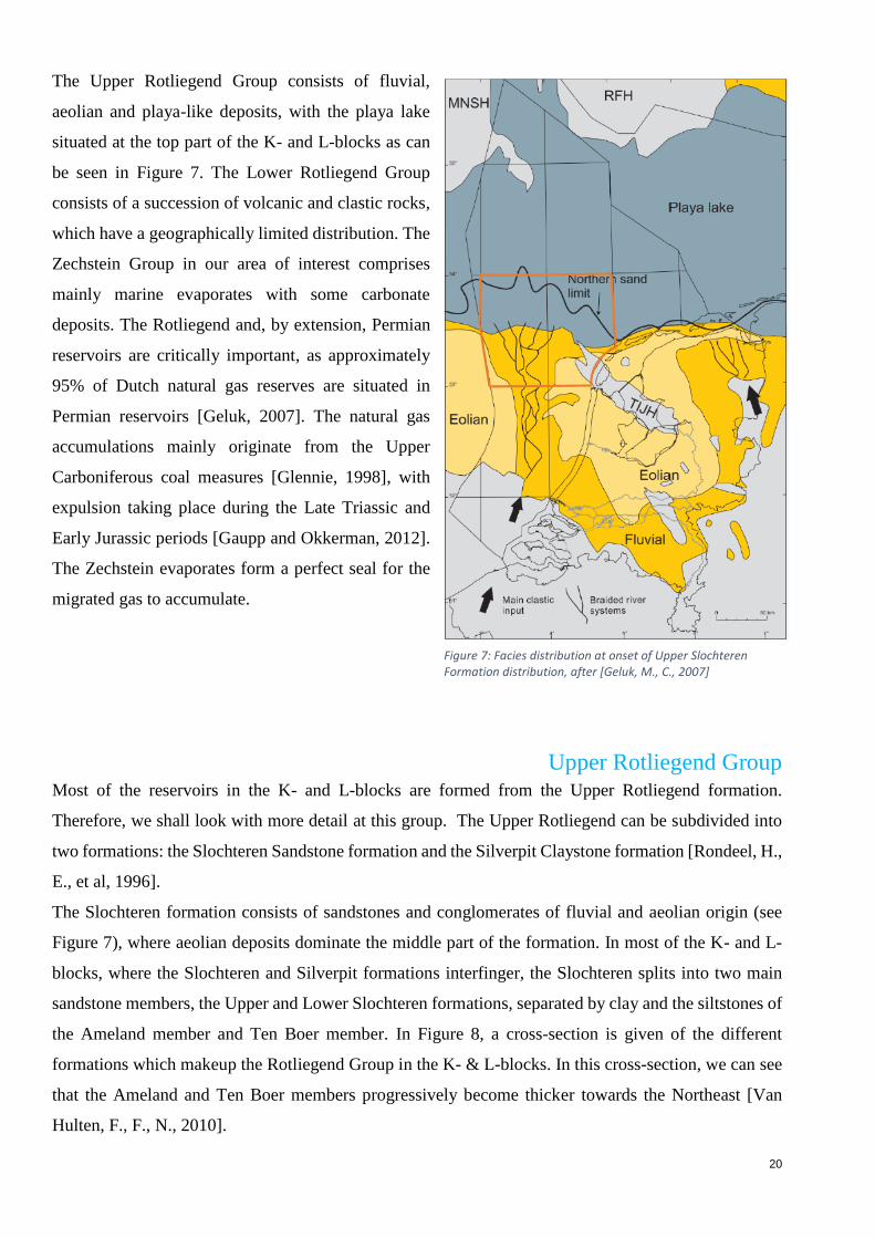
The Upper Rotliegend Group consists of fluvial,

aeolian and playa-like deposits, with the playa lake

situated at the top part of the K- and L-blocks as can

be seen in Figure 7. The Lower Rotliegend Group

consists of a succession of volcanic and clastic rocks,

which have a geographically limited distribution. The

Zechstein Group in our area of interest comprises

mainly marine evaporates with some carbonate

deposits. The Rotliegend and, by extension, Permian

reservoirs are critically important, as approximately

95% of Dutch natural gas reserves are situated in

Permian reservoirs [Geluk, 2007]. The natural gas

accumulations mainly originate from the Upper

Carboniferous coal measures [Glennie, 1998], with

expulsion taking place during the Late Triassic and

Early Jurassic periods [Gaupp and Okkerman, 2012].

The Zechstein evaporates form a perfect seal for the

migrated gas to accumulate.

Upper Rotliegend Group Most of the reservoirs in the K- and L-blocks are formed from the Upper Rotliegend formation.

Therefore, we shall look with more detail at this group. The Upper Rotliegend can be subdivided into

two formations: the Slochteren Sandstone formation and the Silverpit Claystone formation [Rondeel, H.,

E., et al, 1996].

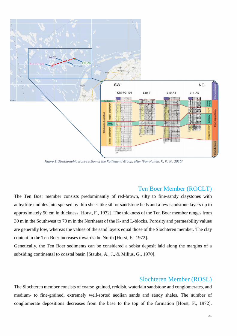
The Slochteren formation consists of sandstones and conglomerates of fluvial and aeolian origin (see

Figure 7), where aeolian deposits dominate the middle part of the formation. In most of the K- and L-

blocks, where the Slochteren and Silverpit formations interfinger, the Slochteren splits into two main

sandstone members, the Upper and Lower Slochteren formations, separated by clay and the siltstones of

the Ameland member and Ten Boer member. In Figure 8, a cross-section is given of the different

formations which makeup the Rotliegend Group in the K- & L-blocks. In this cross-section, we can see

that the Ameland and Ten Boer members progressively become thicker towards the Northeast [Van

Hulten, F., F., N., 2010].

Figure 7: Facies distribution at onset of Upper Slochteren Formation distribution, after [Geluk, M., C., 2007]

21

Ten Boer Member (ROCLT) The Ten Boer member consists predominantly of red-brown, silty to fine-sandy claystones with

anhydrite nodules interspersed by thin sheet-like silt or sandstone beds and a few sandstone layers up to

approximately 50 cm in thickness [Horst, F., 1972]. The thickness of the Ten Boer member ranges from

30 m in the Southwest to 70 m in the Northeast of the K- and L-blocks. Porosity and permeability values

are generally low, whereas the values of the sand layers equal those of the Slochteren member. The clay

content in the Ten Boer increases towards the North [Horst, F., 1972].

Genetically, the Ten Boer sediments can be considered a sebka deposit laid along the margins of a

subsiding continental to coastal basin [Staube, A., J., & Milius, G., 1970].

Slochteren Member (ROSL) The Slochteren member consists of coarse-grained, reddish, waterlain sandstone and conglomerates, and

medium- to fine-grained, extremely well-sorted aeolian sands and sandy shales. The number of

conglomerate depositions decreases from the base to the top of the formation [Horst, F., 1972].

Figure 8: Stratigraphic cross-section of the Rotliegend Group, after [Van Hulten, F., F., N., 2010]

22

Permeabilities in the sand range from 0.1 to 1 Darcy with occasional streaks of high permeabilities of

up to 3 Darcy. The in situ porosities vary from 15% to 20% [Staube, A., J., & Milius, G., 1970]. The

sediments can be subdivided into two genetic groups: fluviatile conglomerates and sandstones, which

are wadi deposits and predominate in the lower part of the member, and aeolian sandstones, which are

deposited in arid conditions. The conglomerate rock fragments comprise metamorphic and volcanic

rocks [Horst, F., 1972].

Ameland Member (ROCLA) Red to red-brown shales and siltstones, often sandy, with thin sandstone beds intercalated, characterise

the Ameland member. Small anhydrite nodules are common [Falke, H., 1975]. Locally, the

Carboniferous can directly underlie the Ameland, but typically, the well-developed sandstones of the

Lower Slochteren underlie it [Falke, H., 1975].

Structural Geology

Rotliegend gas fields often show a discrepancy between the static gas initially in place (GIIP) volumes

and the volumes which can be derived from material balance calculations during/after production

[Frikken & Stark, 1993; Molen et al., 2003; Zijlstra et al., 2007]. The structural geology of the reservoirs

can shed a light on these discrepancies. The majority of Rotliegend traps exist from a dipping fault block

bounded by two or more faults which define the reservoir dimensions. This is comparable to the majority

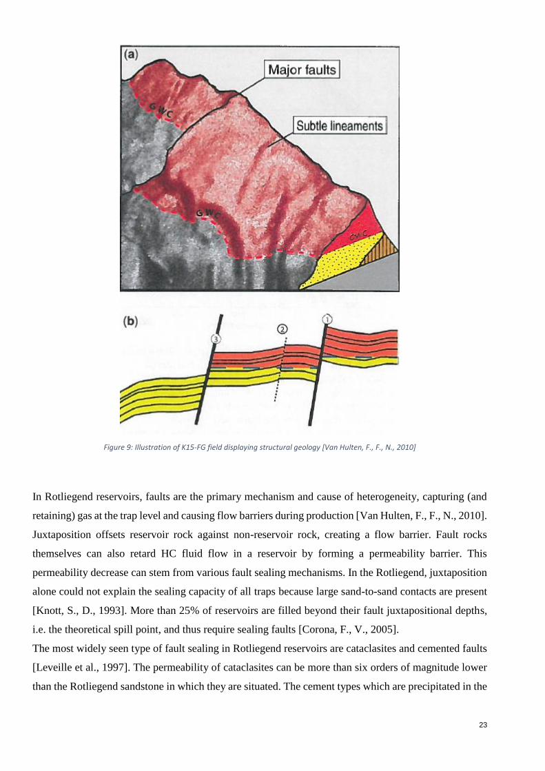
of structural traps in the northern North Sea [Knott, S. D. 1993]. In Figure 9 (a), an illustration is given

of the K15-FG field. A number of faults and subtle lineaments intersect this field and influence its fluid

flow characteristics. In Figure 9 (b), we can see two main faults wherein sand-to-sand sealing behaviour

is the cause of a different GWC different depth, i.e. compartmentalisation.

23

Figure 9: Illustration of K15-FG field displaying structural geology [Van Hulten, F., F., N., 2010]

In Rotliegend reservoirs, faults are the primary mechanism and cause of heterogeneity, capturing (and

retaining) gas at the trap level and causing flow barriers during production [Van Hulten, F., F., N., 2010].

Juxtaposition offsets reservoir rock against non-reservoir rock, creating a flow barrier. Fault rocks

themselves can also retard HC fluid flow in a reservoir by forming a permeability barrier. This

permeability decrease can stem from various fault sealing mechanisms. In the Rotliegend, juxtaposition

alone could not explain the sealing capacity of all traps because large sand-to-sand contacts are present

[Knott, S., D., 1993]. More than 25% of reservoirs are filled beyond their fault juxtapositional depths,

i.e. the theoretical spill point, and thus require sealing faults [Corona, F., V., 2005].

The most widely seen type of fault sealing in Rotliegend reservoirs are cataclasites and cemented faults

[Leveille et al., 1997]. The permeability of cataclasites can be more than six orders of magnitude lower

than the Rotliegend sandstone in which they are situated. The cement types which are precipitated in the

24

faults consist of a wide variety of minerals, including the following: anhydrite, ankerite, barite, siderite

and sphalerite [Leveille et al., 1997]. However, the permeability decrease of most faults is not large

enough to hinder HC flow, and certainly not on a geological timescale. More than 80% of faults in the

siliciclastic petroleum reservoirs in the North Sea cannot retard fluid on a km scale. Nevertheless, faults

can retard flow due to wetting behaviour. In water-wet reservoirs, faults can not only retard flow but

also act as absolute barriers. The buoyancy force has to exceed the capillary entry pressure for flow to

occur. Once this entry pressure has been exceeded, the permeability of the fault rock becomes the main

driver of the fluid flow. At low HC saturations, the entry pressure of the faults is inversely related to

their permeametry in the log-log space [Pìttman, 1992].

The most widely used methods for measuring and determining fault sealing behaviour (e.g. CSP, SSF,

SGR) are based on the distributed amount of shale in the fault. It is important to note that despite the

importance of fault sealing behaviour, the literature lacks definitive models which can be used to assess

why a fault can retard flow in a certain geological setting but act as a conduit in other circumstances. A

large contribution to the lack of accuracy of these models is the extreme complexity of fault zones in the

subsurface. One of these complexities is, for instance, sedimentary heterogeneities. These could also be

the cause of a difference of the oil-water contact (OWC)/ GWC, and not faults [Fisher, Q., J., 2001].

In the report of the Rock Deformation Group [Fisher, Q., J., 2006] on the impact of faults on fluid flow

in the Slochteren, most differences in GWCs in intra-reservoir faults stem from the presence of stranded

(or perched) water. An important implication of this is that when different wells in the same reservoir

have different GWC heights, this cannot be used as a strong indication of compartmentalisation within

that reservoir.

Near the FWL, the buoyancy force of the hydrostatic column is insufficient for overcoming the capillary

entry pressure of the fault. The relative permeability of the gas is therefore zero. However, when the

height of the hydrostatic column increases above the FWL and the buoyancy force also increases, the

buoyancy force reaches a point where it is larger than the capillary entry pressure. Flow across the fault

rock is now determined based on its permeability.

This means that faults which are relatively close to the FWL (e.g. close to the edge of the structure) can

behave as absolute flow barriers, whereas the same faults at the top of the structure do not [Fisher, Q.,

J., 2006].

Reservoir Characteristics

The Slochteren formation is identified as a fine- to medium-grained sandstone [Horst, F., 1972]. The

typical pore throat diameter range lies in the range of 9.00 µm – 23.00 µm [Nelson, P., H., 2009]. The

25

Ameland and Ten Boer formations are identified as course siltstones [Horst, F., 1972]. Their pore throat

diameter range typically is in the range of 4.00 µm – 7.00 µm. In Table 2, typical pore throat diameters

have been given for various types of reservoirs.

Table 2: Summary of typical pore throat size and reservoir parameters for siliciclastic rocks [Nelson, P.,H., 2009]

Source of Samples Pore Throat Diameters (µm) Porosity

%

Permeability

mD

Depth

TVDSS

m

Min. Max. Avg.

Medium-grained sandstones,

various, worldwide

9 23 16.7 14 25.5 2000

Fine-grained sandstones, various,

worldwide

4 30 15.5 18.1 19.6 2000

Very fine-grained sandstones,

various, worldwide

8 13 9.7 24.2 109.7 2000

Coarse siltstones, various,

worldwide

4 7 5.7 26.3 22.3 2000

Because different gas mixtures are present in reservoirs of the K- and L-blocks, various gas compositions

have been used. The interfacial tension (IFT) range of a gas mixture with a varying composition has

been determined for typical Slochteren (siliciclastic) reservoir parameters as 25 – 45 dynes/cm (= 0.025

– 0.045 N/m) [Rushing, J., A., et al., 2008]. The gas mixture properties which have been used to

determine the gas-water IFT interval are given in Table 3.

Table 3: Gas compositions for gas-water IFT range [Rushing, J., A., et al., 2008]

Composition Gas 1

mol%

Gas 2

mol%

Gas 3

mol%

Gas 4

mol%

Gas 5

mol%

Gas 6

mol%

Gas 7

mol%

Methane 96.00 91.20 86.4 76.8 91.2 86.4 76.8

Ethane 3.00 2.85 2.70 2.40 2.85 2.70 2.40

Propane 1.00 0.95 0.90 0.80 0.95 0.90 0.80

Nitrogen 0.00 0.00 0.00 0.00 5.00 10.00 20.00

Carbon Dioxide 0.00 5.00 10.00 20.00 0.00 0.00 0.00

Total mol% 100.00 100.00 100.00 100.00 100.00 100.00 100.00

HC mol% 100.00 100.00 100.00 100.00 100.00 100.00 100.00

Total Gas Specific

Gravity, ɣg

0.5781 0.6252 0.6723 0.7664 0.5976 0.617 0.656

Hydrocarbon

Specific Gravity, ɣHC

0.5781 0.5781 0.5781 0.5781 0.5781 0.5781 0.5781

26

Hydrocarbon Contact Database

Methodology To assess the significance of HC contact depth in support of petroleum exploration, an extensive

knowledge of subsurface contacts is required. In the chapter Definitions of Terms definitions have been

given for the GWC, FWL and their relevance. To facilitate this research, a HC contact database was

created with data from 122 gas fields. A table with all of the data sets can be found in Appendix A.

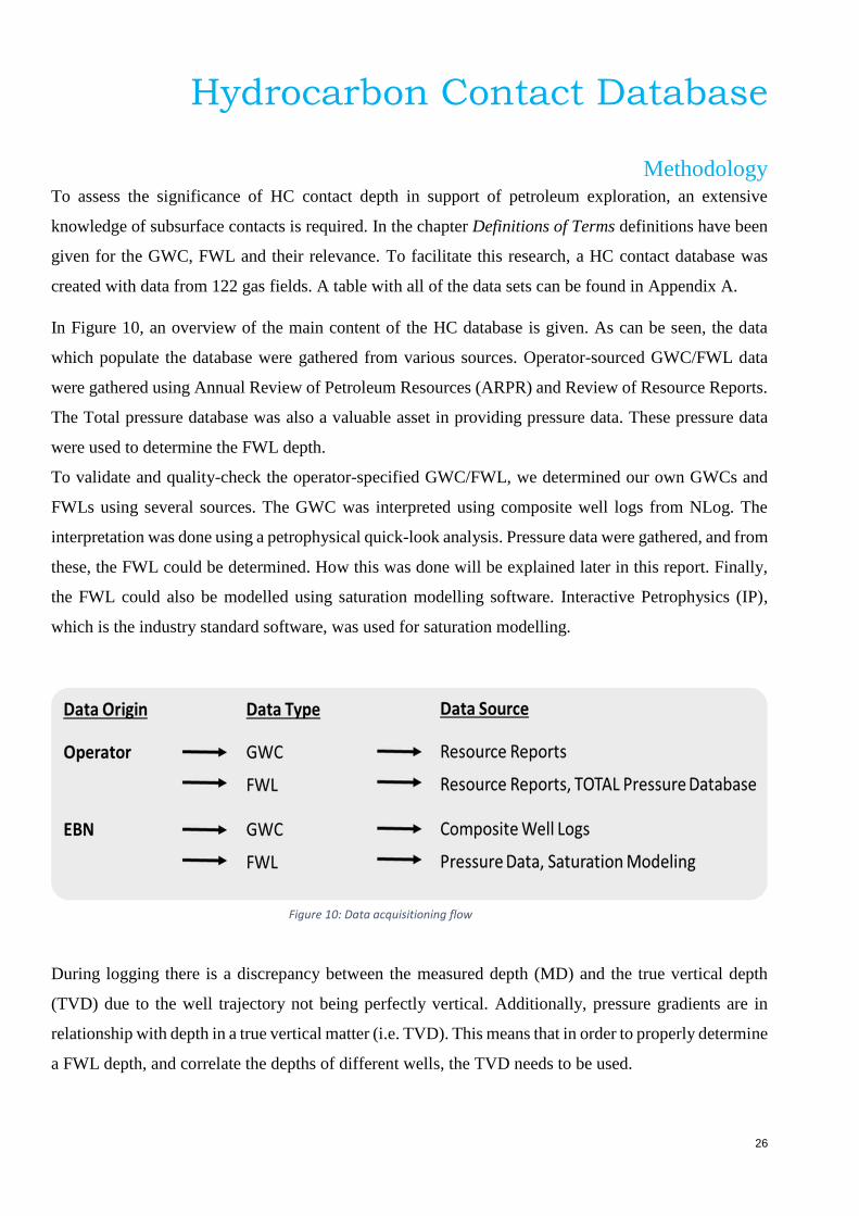
In Figure 10, an overview of the main content of the HC database is given. As can be seen, the data

which populate the database were gathered from various sources. Operator-sourced GWC/FWL data

were gathered using Annual Review of Petroleum Resources (ARPR) and Review of Resource Reports.

The Total pressure database was also a valuable asset in providing pressure data. These pressure data

were used to determine the FWL depth.

To validate and quality-check the operator-specified GWC/FWL, we determined our own GWCs and

FWLs using several sources. The GWC was interpreted using composite well logs from NLog. The

interpretation was done using a petrophysical quick-look analysis. Pressure data were gathered, and from

these, the FWL could be determined. How this was done will be explained later in this report. Finally,

the FWL could also be modelled using saturation modelling software. Interactive Petrophysics (IP),

which is the industry standard software, was used for saturation modelling.

During logging there is a discrepancy between the measured depth (MD) and the true vertical depth

(TVD) due to the well trajectory not being perfectly vertical. Additionally, pressure gradients are in

relationship with depth in a true vertical matter (i.e. TVD). This means that in order to properly determine

a FWL depth, and correlate the depths of different wells, the TVD needs to be used.

Figure 10: Data acquisitioning flow

27

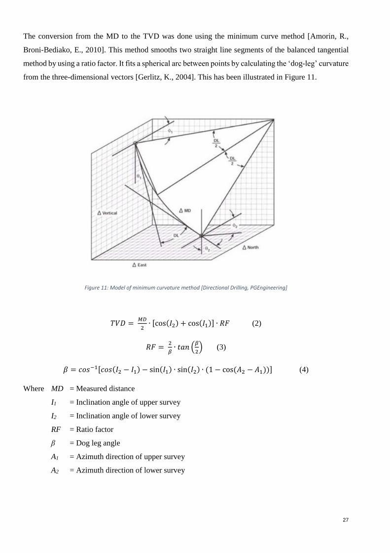
The conversion from the MD to the TVD was done using the minimum curve method [Amorin, R.,

Broni-Bediako, E., 2010]. This method smooths two straight line segments of the balanced tangential

method by using a ratio factor. It fits a spherical arc between points by calculating the ‘dog-leg’ curvature

from the three-dimensional vectors [Gerlitz, K., 2004]. This has been illustrated in Figure 11.

Figure 11: Model of minimum curvature method [Directional Drilling, PGEngineering]

𝑇𝑉𝐷 = 𝑀𝐷

2∙ [cos(𝐼2) + cos(𝐼1)] ∙ 𝑅𝐹 (2)

𝑅𝐹 = 2

𝛽∙ 𝑡𝑎𝑛 (

𝛽

2) (3)

𝛽 = 𝑐𝑜𝑠−1[𝑐𝑜𝑠(𝐼2 − 𝐼1) − sin(𝐼1) ∙ sin(𝐼2) ∙ (1 − cos (𝐴2 − 𝐴1))] (4)

Where MD = Measured distance

I1 = Inclination angle of upper survey

I2 = Inclination angle of lower survey

RF = Ratio factor

β = Dog leg angle

A1 = Azimuth direction of upper survey

A2 = Azimuth direction of lower survey

28

The log evaluation of composite well log data was done using a quick-look petrophysical analysis. A

quick-look petrophysical analysis typically tries to solve a system of log responses, i.e. gamma ray (GR),

density and resistivity in a composite well log. In this thesis it is used to determine the GWC. The quick-

look approach is well documented in standard texts on log evaluation such as Petrophysics: A Practical

Guide [Cannon, S., 2015]. An example of a composite well log with typical transition behaviour has

been given in Figure 12. At the depth of the GWC at approximately 3210 m TVD subsea (TVDSS), the

deep resistivity log shows a gradual decrease in value, whereas the gamma ray remains constant,

indicating that no change in lithology takes place. This is indicative of a phase transition zone, i.e. a

GWC. The decrease of the RES log is caused by the fact that pores that are filled with hydrocarbons are

less resistive than surrounding saline ground water.

Figure 12: Composite well log of well K07-10

29

The FWL is determined using pressure data. The hydrostatic pressure equation, 𝑃 = 𝜌 ∙ 𝑔 ∙ 𝑧, is used to

calculate pressures in the subsurface. A significant difference exists between the density (ρ) of water and

the density of gas. Therefore, the pressure plots of both phases have a significantly different gradient.

The point where the pressure plot changes its gradient is the FWL. As an example, the RFT pressure

data of well K07-10 has been plotted against the TVDSS in Figure 13. An FWL can be interpreted where

the gas pressure line and water pressure line intersect.

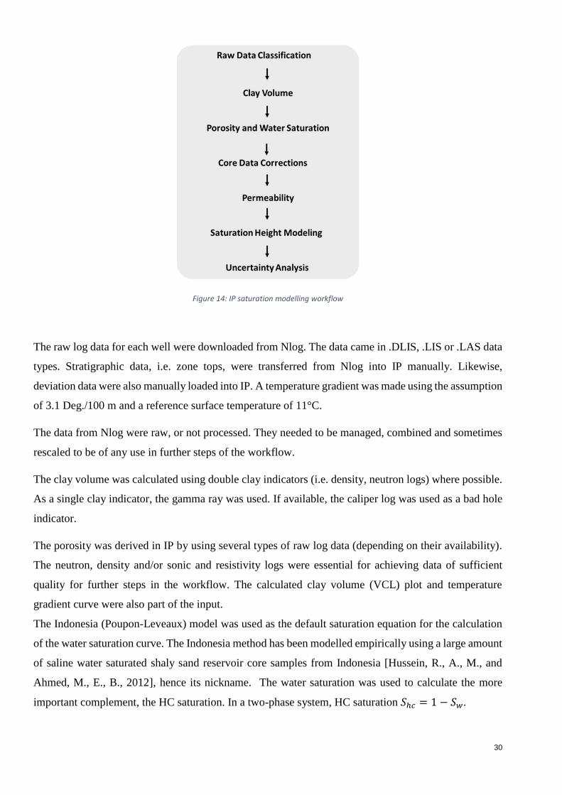
A more theoretical way of determining the FWL in a reservoir is to model it. The FWL and its uncertainty

can be calculated by using modelling software. Interactive Petrophysics (IP) was used to determine the

FWL of 24 wells and to perform an uncertainty analysis of these wells. A typical workflow has been

given in Figure 14. The workflow was repeated for every single well, and takes approximately one day

per well. In the next paragraph, each of the steps will be briefly explained, and the main assumptions of

each step will be reported.

3100

3150

3200

3250

3300

3350

3400

310 320 330 340 350 360

Dep

th T

VD

SS [

m]

Pressure [bar]

RFT pressure data, Well K07-10, 1996

Pressure Data

Hydrostatic Pressure

Gas Pressure Line

Water Pressure Line

Figure 13: Pressure data of well K07-10

30

Figure 14: IP saturation modelling workflow

The raw log data for each well were downloaded from Nlog. The data came in .DLIS, .LIS or .LAS data

types. Stratigraphic data, i.e. zone tops, were transferred from Nlog into IP manually. Likewise,

deviation data were also manually loaded into IP. A temperature gradient was made using the assumption

of 3.1 Deg./100 m and a reference surface temperature of 11°C.

The data from Nlog were raw, or not processed. They needed to be managed, combined and sometimes

rescaled to be of any use in further steps of the workflow.

The clay volume was calculated using double clay indicators (i.e. density, neutron logs) where possible.

As a single clay indicator, the gamma ray was used. If available, the caliper log was used as a bad hole

indicator.

The porosity was derived in IP by using several types of raw log data (depending on their availability).

The neutron, density and/or sonic and resistivity logs were essential for achieving data of sufficient

quality for further steps in the workflow. The calculated clay volume (VCL) plot and temperature

gradient curve were also part of the input.

The Indonesia (Poupon-Leveaux) model was used as the default saturation equation for the calculation

of the water saturation curve. The Indonesia method has been modelled empirically using a large amount

of saline water saturated shaly sand reservoir core samples from Indonesia [Hussein, R., A., M., and

Ahmed, M., E., B., 2012], hence its nickname. The water saturation was used to calculate the more

important complement, the HC saturation. In a two-phase system, HC saturation 𝑆ℎ𝑐 = 1 − 𝑆𝑤.

31

The Indonesia (Poupon-Leveaux) model was chosen because it is useful in sandstone but also shale

intervals [Moradzadeh, A., 2011]. This method has been used because of the relative high shale content

in the intervals at the FWL depth of the selected wells for saturation modelling. It is an empirical model,

and thus, the detailed functionality for HC-bearing sands is unsupported except for by common sense

and longstanding use.

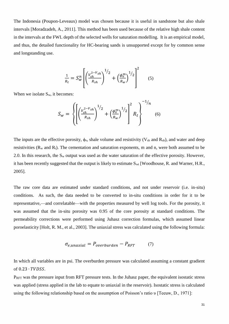
1

𝑅𝑡= 𝑆𝑤

𝑛 [(𝑉𝑠ℎ

2−𝑉𝑠ℎ

𝑅𝑠ℎ)

12⁄

+ (𝜙𝑒

𝑚

𝑅𝑤)

12⁄

]

2

(5)

When we isolate Sw, it becomes:

𝑆𝑤 = {[(𝑉𝑠ℎ

2−𝑉𝑠ℎ

𝑅𝑠ℎ)

12⁄

+ (𝜙𝑒

𝑚

𝑅𝑤)

12⁄

]

2

𝑅𝑡}

−1𝑛⁄

(6)

The inputs are the effective porosity, ϕe, shale volume and resistivity (Vsh and Rsh), and water and deep

resistivities (Rw and Rt). The cementation and saturation exponents, m and n, were both assumed to be

2.0. In this research, the Sw output was used as the water saturation of the effective porosity. However,

it has been recently suggested that the output is likely to estimate Swt [Woodhouse, R. and Warner, H.R.,

2005].

The raw core data are estimated under standard conditions, and not under reservoir (i.e. in-situ)

conditions. As such, the data needed to be converted to in-situ conditions in order for it to be

representative,—and correlatable—with the properties measured by well log tools. For the porosity, it

was assumed that the in-situ porosity was 0.95 of the core porosity at standard conditions. The

permeability corrections were performed using Juhasz correction formulas, which assumed linear

poroelasticity [Holt, R. M., et al., 2003]. The uniaxial stress was calculated using the following formula:

𝜎𝑒,𝑢𝑛𝑎𝑥𝑖𝑎𝑙 = 𝑃𝑜𝑣𝑒𝑟𝑏𝑢𝑟𝑑𝑒𝑛 − 𝑃𝑅𝐹𝑇 (7)

In which all variables are in psi. The overburden pressure was calculated assuming a constant gradient

of 0.23 ∙ 𝑇𝑉𝐷𝑆𝑆.

PRFT was the pressure input from RFT pressure tests. In the Juhasz paper, the equivalent isostatic stress

was applied (stress applied in the lab to equate to uniaxial in the reservoir). Isostatic stress is calculated

using the following relationship based on the assumption of Poisson’s ratio υ [Teeuw, D., 1971]:

32

𝜎𝑖𝑠𝑜 = 1

3

(1+𝜐)

(1−𝜐)𝜎𝑒,𝑢𝑛𝑎𝑥𝑖𝑎𝑙 (8)

The possions ratio υ was assumed to be 0.2. This was based on the values for a typical sandstone which

Fjaer stipulated [Fjaer, E., 2008].

In order to calculate a permeability curve in IP, determining a porosity permeability relationship based

on Reduced Major Axis (RMA) regression can be used. With this relationship, we can create a

permeability log based on the continuous porosity log (which was created during one of the earlier

workflow steps). When applying a single relationship to derive a porosity-permeability relationship,

without uncertainty bands, RMA has been used, since the regression utilizes 2 linearly distributed

variables and the residuals are the smallest.

The RMA has been utilized assuming that the sandstone interval in the reservoir is homogeneous. As a

reservoir in real life is never completely homogeneous, a relationship which accounts for the inherent

heterogeneity of the dataset is preferred. However, such a relationship is not easily made in IP, therefore,

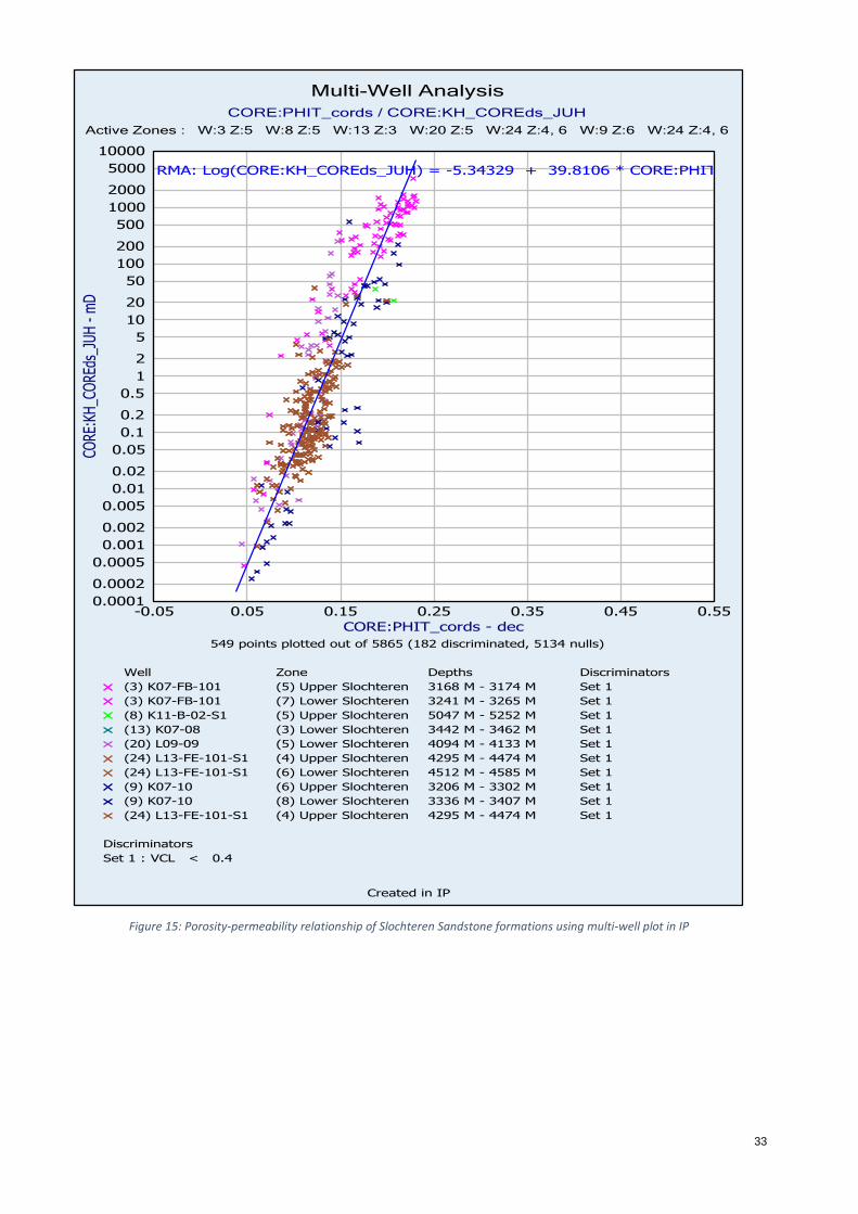
we opted for an RMA relationship instead. In Figure 15, a multi-well plot of the Upper and Lower

Slochteren members has been given in which a porosity-permeability relationship has been established.

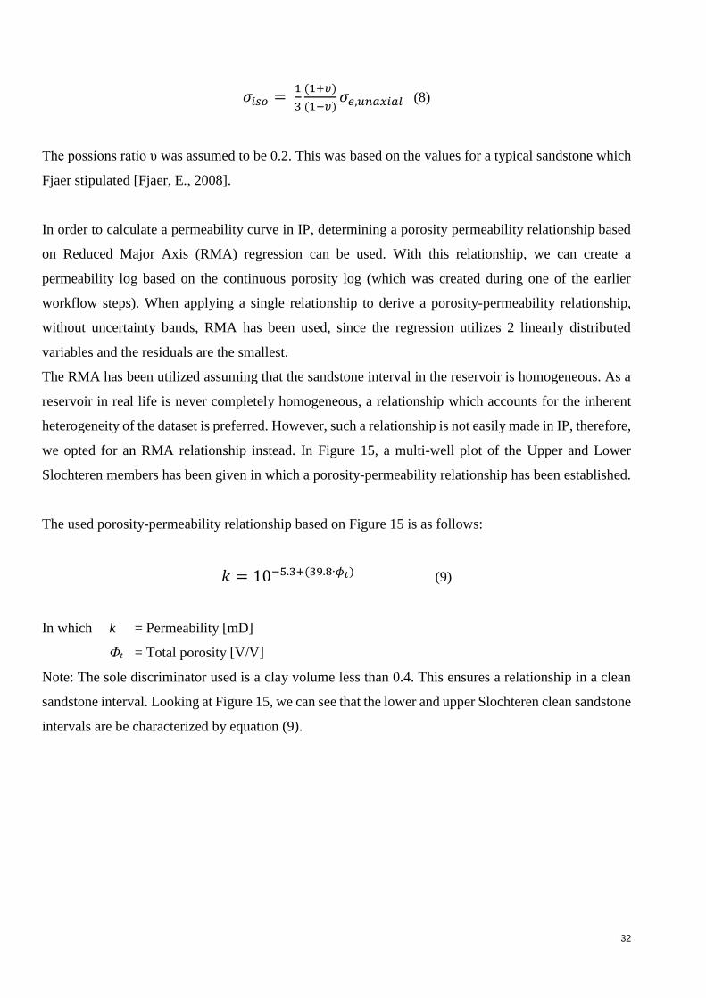
The used porosity-permeability relationship based on Figure 15 is as follows:

𝑘 = 10−5.3+(39.8∙𝜙𝑡) (9)

In which k = Permeability [mD]

Φt = Total porosity [V/V]

Note: The sole discriminator used is a clay volume less than 0.4. This ensures a relationship in a clean

sandstone interval. Looking at Figure 15, we can see that the lower and upper Slochteren clean sandstone

intervals are be characterized by equation (9).

33

Figure 15: Porosity-permeability relationship of Slochteren Sandstone formations using multi-well plot in IP

34

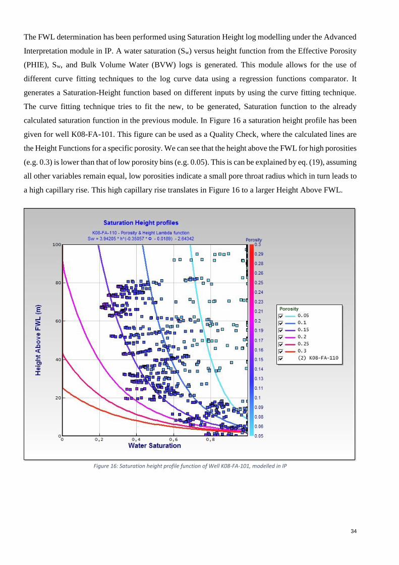
The FWL determination has been performed using Saturation Height log modelling under the Advanced

Interpretation module in IP. A water saturation (Sw) versus height function from the Effective Porosity

(PHIE), Sw, and Bulk Volume Water (BVW) logs is generated. This module allows for the use of

different curve fitting techniques to the log curve data using a regression functions comparator. It

generates a Saturation-Height function based on different inputs by using the curve fitting technique.

The curve fitting technique tries to fit the new, to be generated, Saturation function to the already

calculated saturation function in the previous module. In Figure 16 a saturation height profile has been

given for well K08-FA-101. This figure can be used as a Quality Check, where the calculated lines are

the Height Functions for a specific porosity. We can see that the height above the FWL for high porosities

(e.g. 0.3) is lower than that of low porosity bins (e.g. 0.05). This is can be explained by eq. (19), assuming

all other variables remain equal, low porosities indicate a small pore throat radius which in turn leads to

a high capillary rise. This high capillary rise translates in Figure 16 to a larger Height Above FWL.

Figure 16: Saturation height profile function of Well K08-FA-101, modelled in IP

35

Finally, using the generated Saturation Height Function we can try to find the FWL using the ‘FWL

Finder’ function in IP to predict the FWL based on the least error margin method. Here the calculator

automatically varies the FWL depth in order to get the best fit estimate based on the least error between

the originally calculated water saturation and the new generated water saturation based on the Saturation

Height function. In track 4 (which has been highlighted in yellow) in Figure 17, the blue curve is the

original calculated water saturation (from the Indonesian method) and the red curve is the new generated

saturation function. It can be seen clearly that there is a good fit between both saturations, hence the

saturation height function is verified, and can be used for a FWL estimation.

Figure 17: Interactive Log plot used to calculate the FWL of Well K08-FA-110, modelled in IP

Uncertainty Analysis

In this chapter, the results of an uncertainty analysis are presented, including a quantification of depth

measurement uncertainty using literature data and the results from this study. Their contributions to a

global error are described. A theoretical uncertainty range is derived for capillary pressure

measurements, and a sensitivity analysis is done for capillary entry height.

36

Sources of Petrophysical Uncertainty The most important reservoir parameters (i.e. K, Sw) are not directly measured with well logging. Rather,

they are indirectly derived through the use of multiple steps, including interpretation, processing and

calibration. This means they are inherently subject to inaccuracies stemming from uncertainties in the

well logs. It is critical to analyse and qualify these uncertainties. A qualification of the main uncertainties

has been given in the work of W.R. William et al. [W.R. William et al., 2011]. As an example, the

implication of uncertainties on a porosity determination in bad borehole conditions has been given in

Figure 28 in Appendix B. The determination of a valuable reservoir parameter, such as permeability, is

error prone and largely depends on the skills of the analyst. These uncertainties can also ultimately affect

the height of the FWL in saturation modelling.

Even direct (raw) log measurements are subject to inaccuracies. The depth measured during a logging

run is one of the main sources of uncertainty [M.H. Rider, 1986]. All log measurements are recorded

against the measured depth along the hole. This depth is usually assumed to be exact; however, it is also

subject to uncertainty in different ways. For instance, tension in the cables due to the weight of the

logging tool causes the cable to extend and contract. Fortunately, the uncertainty in depth measurements

can be quantified. In the work of Hall [Hall, M., 2012], this uncertainty has been named the uncertainty

ellipsoid (see Figure 18).

Figure 18: Uncertainty in depth measurements [Hall,M., 2012]

37

This report will quantify the uncertainty in two ways. The first is with a theoretical derivation of the

depth measurement uncertainty using values obtained from [Theys, 1991 and Søllie and Rodgers, 1994].

The quantification is done using Gaussian error propagation. The second method is a more hands-on

approach where the depth difference of multiple logging runs in a specific well are compared with each

other. The offset of these logs, i.e. the depth shift, is indicative of the error in depth measurement.

Quantification of Wireline Depth Measurement Uncertainty

Gaussian Error Propagation

Gaussian Error Propagation is used to analytically determine the global uncertainty (or error) produced

by multiple, and interacting, measurements or variables. As such, the technique is useful in cases where

step-by-step calculations are performed in which each step provides an inherent uncertainty [Lo, E,

2005].

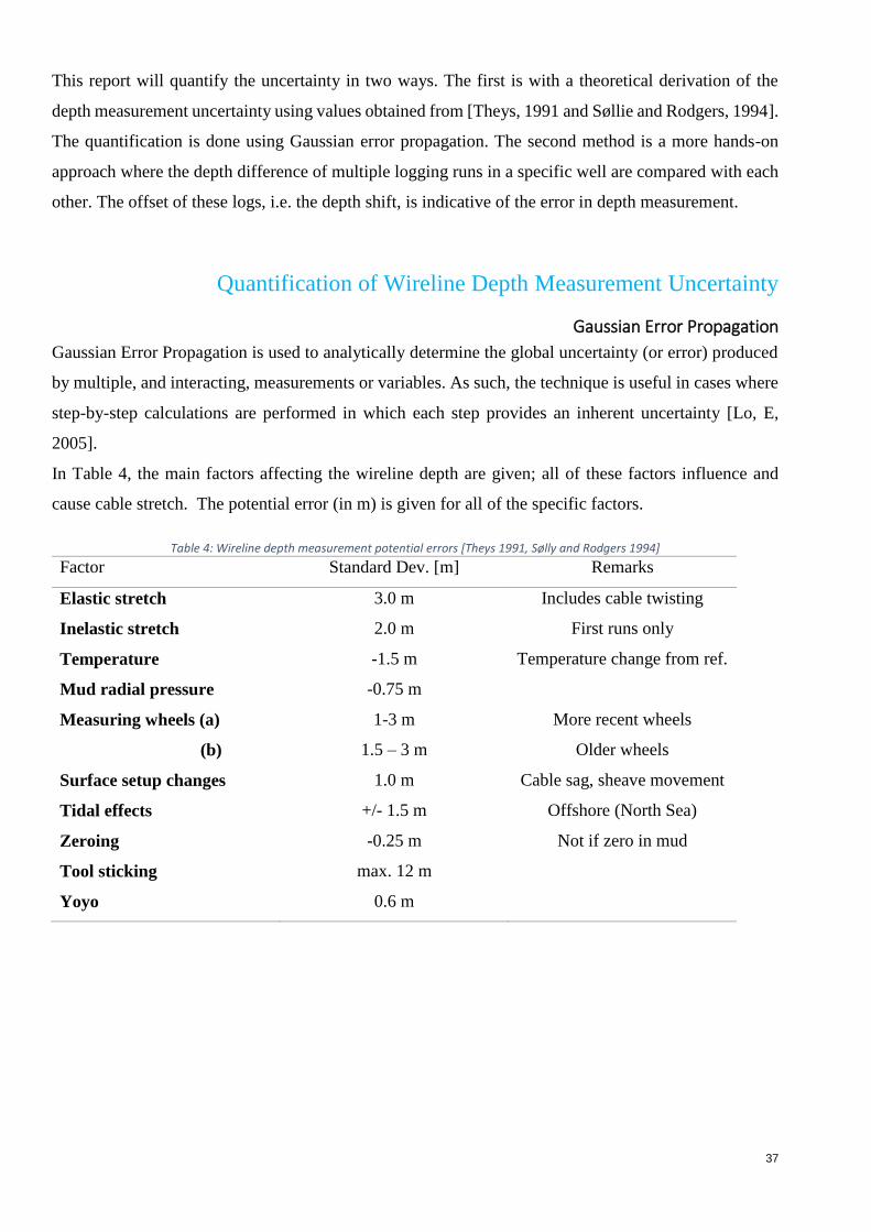
In Table 4, the main factors affecting the wireline depth are given; all of these factors influence and

cause cable stretch. The potential error (in m) is given for all of the specific factors.

Table 4: Wireline depth measurement potential errors [Theys 1991, Sølly and Rodgers 1994]

Factor Standard Dev. [m] Remarks

Elastic stretch

Inelastic stretch

Temperature

Mud radial pressure

Measuring wheels (a)

(b)

Surface setup changes

Tidal effects

Zeroing

Tool sticking

Yoyo

3.0 m

2.0 m

-1.5 m

-0.75 m

1-3 m

1.5 – 3 m

1.0 m

+/- 1.5 m

-0.25 m

max. 12 m

0.6 m

Includes cable twisting

First runs only

Temperature change from ref.

More recent wheels

Older wheels

Cable sag, sheave movement

Offshore (North Sea)

Not if zero in mud

38

To determine the global error, we can use the Gaussian equation of error propagation. For addition and

subtraction, the following applies:

If Q is some combination of sums and differences, and 𝑎 is a variable with a local uncertainty 𝑥 , i.e.

𝑄 = ∑ |𝑥𝑖|𝑧𝑖=𝑎 (10)

then

𝛿𝑄 = √∑ (𝛿𝑥𝑖)2𝑧𝑖=𝑎 (11)

This means that global uncertainty 𝛿𝑄 is equal to the square root of the sum of the squares of all of the

‘local’ errors. When applying this formula to Table 4, we get 𝛿𝑄 = 12.9 𝑚. When we disregard the

uncertainty of tool sticking, we get 𝛿𝑄 = 4.8 𝑚.

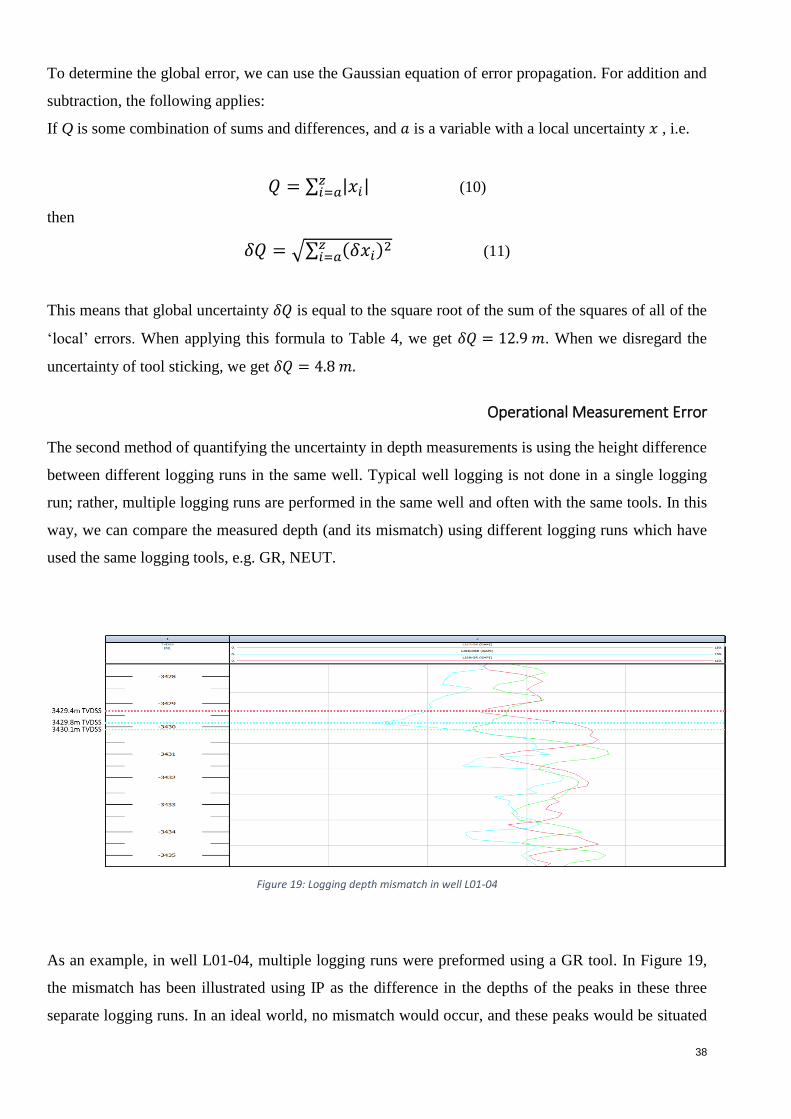
Operational Measurement Error

The second method of quantifying the uncertainty in depth measurements is using the height difference

between different logging runs in the same well. Typical well logging is not done in a single logging

run; rather, multiple logging runs are performed in the same well and often with the same tools. In this

way, we can compare the measured depth (and its mismatch) using different logging runs which have

used the same logging tools, e.g. GR, NEUT.

Figure 19: Logging depth mismatch in well L01-04

As an example, in well L01-04, multiple logging runs were preformed using a GR tool. In Figure 19,

the mismatch has been illustrated using IP as the difference in the depths of the peaks in these three

separate logging runs. In an ideal world, no mismatch would occur, and these peaks would be situated

39

on top of one another at the exact same depth. Using the maximum difference as 𝛿𝑄, we see that 𝛿𝑄 =

3430 − 3429 = 1 m. This is much less than the theoretical 𝛿𝑄 of 4.8 m due to the fact that not all of

the factors which can affect the wireline depth measurements are always present. Therefore, the

theoretical 𝛿𝑄 value of 4.8 m should be used as a maximum potential error.

Sensitivity Analysis of Capillary Rise

Gaussian Error Propagation

Gaussian error propagation can also be a valuable tool for a sensitivity study. The height difference

between the FWL and (in our case) the GWC is in porous media an effect of the capillary rise. The

formula for Pc can be analysed using Gaussian error propagation.

If ∆𝑃𝑐 = 𝑃𝑊 − 𝑃𝑁𝑊 = ∆𝜌𝑔ℎ =2 𝜎 𝑐𝑜𝑠𝜃

𝑅 (12)

We can simplify this with the following equation:

𝑈 = 𝑥𝑦

𝑧 (13)

Where 𝑥 = 𝜎, 𝑦 = 𝜃 𝑎𝑛𝑑 𝑧 = 𝑅, now

𝛿𝑈 = √(𝑦

𝑧𝛿𝑥)

2

+ (𝑥

𝑧𝛿𝑦)

2

+ (−𝑥𝑦

𝑧2 𝛿𝑥)2

(14)

(𝛿𝑈)2 = (𝑦

𝑧𝛿𝑥)

2

+ (𝑥

𝑧𝛿𝑦)

2

+ (−𝑥𝑦

𝑧2𝛿𝑥)

2

= (𝑥𝑦

𝑧)

2

[(𝛿𝑥

𝑥)

2

+ (𝛿𝑦

𝑦)

2

+ (−𝛿𝑧

𝑧)

2

] (15)

(𝛿𝑈

𝑈)

2

≈ (𝛿𝑥

𝑥)

2

+ (𝛿𝑦

𝑦)

2

+ (𝛿𝑧

𝑧)

2

(16)

𝛿𝑈 ≈ 𝑈√(𝛿𝑥

𝑥)

2

+ (𝛿𝑦

𝑦)

2

+ (𝛿𝑧

𝑧)

2

(17)

Thus, for the capillary pressure equation, we see that global uncertainty U is equal to U multiplied by

the square root of the sum of the squares of all of the relative errors in the variables. With this knowledge,

we are able to perform a sensitivity analysis of the formula to understand the relationship of the input

variables and the global uncertainty. To do this, we first need to determine a range of plausible values

for the IFT, contact angle and pore throat radius.

40

An IFT range of a gas mixture with a varying composition was determined for typical siliciclastic

reservoir parameters as 25 – 45 dynes/cm (= 0.025 – 0.045 N/m) [Rushing. J., A., et al., 2008]. The gas

mixture properties used to determine the gas-water IFT are given in Table 3. Table 3 also provides a

density range for gas. Using gas specific gravity ɣg, the gas density is defined as the following:

𝜌𝑔𝑎𝑠 = 𝛾𝑔 ∙ 𝜌𝑎𝑖𝑟,𝑠𝑐 (18)

When considering a value range for contact angle θ, we can use the fact that in a silicilastic system,

natural gas is never the wetting phase [Hagoort, J., 1988]. A contact angle range of 0° − 45° as the input

for contact angle θ was used. The pore throat radius of the investigated Rotliegend reservoir can typically

be identified as a medium-grained sandstone. Therefore, the pore throat diameter range is

9.00 µm – 23.00 µm [Nelson, P.,H., 2009]. In Table 2, typical pore throat diameters have been given

for various types of reservoirs.

Monte Carlo Simulation

Using a Monte Carlo simulation, we determined which variable was the most influential in the capillary

rise. The Monte Carlo technique has been chosen because it can model the impact of the different

variables by generating a suite of randomized outcomes for the variables that each have an inherent

uncertainty.

When we solve for ℎ in equation 12, we see that the capillary rise is:

ℎ𝐶𝐴𝑃 =2 𝜎 𝑐𝑜𝑠𝜃

𝑅∆𝜌𝑔 (19)

Where ∆𝜌 is the density difference between the wetting and non-wetting phase. In our case, this was

water and gas. In Table 5, all the used values are summarised.

Table 5: Variable value ranges used for Monte Carlo

Base Low High

σ [N/m] 0.025 0.045

Θ [°] 0 45

Pore Throat Radius [m]

4.50E-06 1.15E-05

∆ρ [kg/m3] 999.29 999.06

g 9.81

41

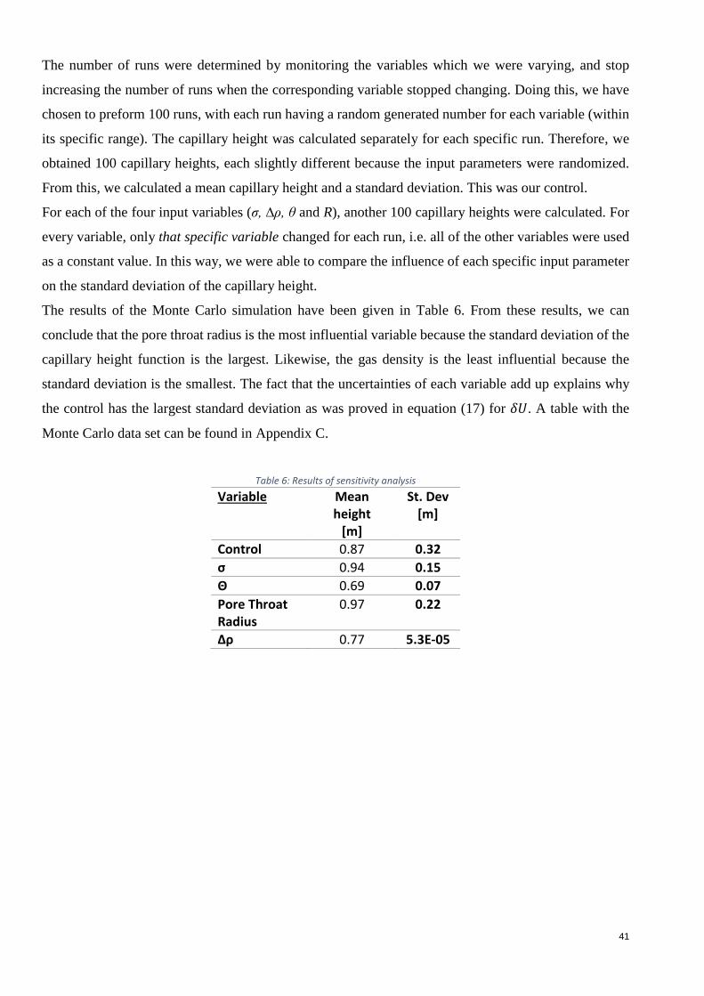
The number of runs were determined by monitoring the variables which we were varying, and stop

increasing the number of runs when the corresponding variable stopped changing. Doing this, we have

chosen to preform 100 runs, with each run having a random generated number for each variable (within

its specific range). The capillary height was calculated separately for each specific run. Therefore, we

obtained 100 capillary heights, each slightly different because the input parameters were randomized.

From this, we calculated a mean capillary height and a standard deviation. This was our control.

For each of the four input variables (σ, ∆ρ, θ and R), another 100 capillary heights were calculated. For

every variable, only that specific variable changed for each run, i.e. all of the other variables were used

as a constant value. In this way, we were able to compare the influence of each specific input parameter

on the standard deviation of the capillary height.

The results of the Monte Carlo simulation have been given in Table 6. From these results, we can

conclude that the pore throat radius is the most influential variable because the standard deviation of the

capillary height function is the largest. Likewise, the gas density is the least influential because the

standard deviation is the smallest. The fact that the uncertainties of each variable add up explains why

the control has the largest standard deviation as was proved in equation (17) for 𝛿𝑈. A table with the

Monte Carlo data set can be found in Appendix C.

Table 6: Results of sensitivity analysis

Variable Mean height

[m]

St. Dev [m]

Control 0.87 0.32

σ 0.94 0.15

Θ 0.69 0.07

Pore Throat Radius

0.97 0.22

∆ρ 0.77 5.3E-05

42

Data Visualisations and Discussion

In this section, the data and results of the HC contact database are visualised and relevant reservoir

properties and parameters are used to analyse the data. Most of the results are displayed using figures

and graphs instead of numbers because it is important to show the areal distribution of the data set. These

results are analysed and their implication for this research are outlined and discussed. Finally, a general

discussion about the research is provided.

Figure 20 displays the locations of the wells and reservoirs which populate the HC contact database. The

data points are colour coded according to the formation in which the FWL is situated, with purple points

representing Triassic reservoirs, green used for Permian basins and yellow used for Carboniferous

reservoirs. The Permian basins form the overwhelming majority with 81% of the 122 data points being

either an Upper or Lower Slochteren Formation. The Carboniferous reservoirs are from the Limburg

Group, and the Triassic reservoirs are Lower Volpriehausen and Solling formations. The age of the

formation containing the FWL increases going westwards. The Triassic formations, being the youngest,

are solely present in the easternmost region of the L- block, whereas the oldest Carboniferous formations

are present solely in the north-western part of the K-block. The Slochteren also displays a clear

separation, with the Upper Slochteren situated more in the southeastern part and the Lower Slochteren

towards the northwest. However, based solely on this data no conclusions can be drawn as to why these

Figure 20: Operator FWL data set of the HC contact database (N= 122)

43

separations exist. An intimate knowledge of the regional geology and geologic history is necessary in

order to explain these separations, that lies beyond the scope of this study.

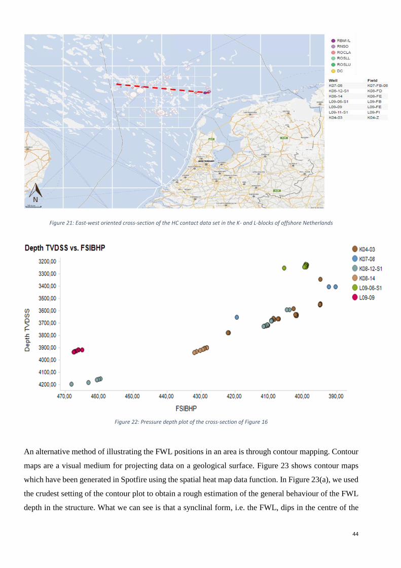
In Figure 21 and Figure 22, an east-west cross section of the K- and L-blocks has been illustrated. Figure

22 visualises the depth pressure plots in bars versus TVDSS. We can see that a general trend in the data

exists from west to east. Moving eastwards, the reservoirs progressively become deeper. However, in

the far eastern area, the reservoir depths become more shallow again. Due to compaction during burial,

the depth of a reservoir has a negative impact on the porosity and pore throat diameter. Empirical linear

best-fit lines show a general decline in porosity with depth [Ramm, M., Bjørlykke, K., 1994]. The decline

in porosity due to compaction can also be illustrated with the HC contact database using the capillary

rise as an analogue. Assuming that all other variables remain constant, we deduct from the capillary

pressure equation (19) that the decrease in porosity leads to a decrease in pore throat radii, which, in

turn, leads to a higher capillary height, i.e. a larger height difference between the GWC and FWL. The

HC contact database was used to analyse this difference. Using data points from reservoirs from the

Upper Slochteren formation, which share the same depositional environment (i.e. playa margin), we

assumed that all of the variables in equation (19) would remain the same except for the pore throat radius.

Two batches were made of the data; we selected reservoirs in which the FWL was less than 3300 m

TVDSS and reservoirs in which the FWL was greater than 3600m TVDSS. These two batches have been

chosen because FWL data was clustered at these depths.

In the batch with FWL less than 3300 m TVDSS, the capillary rise height was approximately 15 m. For

the batch with FWL greater than 3600 m TVDSS, the capillary rise was approximately 18 m. This was

an increase of approximately 24%. Compare this against the linear porosity regression line from Ramm

and Bjørlykke for this interval, where a porosity reduction of 26% is obtained [Ramm, M., Bjørlykke,

K., 1994]. However, these results should be placed into perspective and a disclaimer is due. Assumed is

that depth solely influences the pore throat radius, however depth it is known that depth also changes

other factors such as e.g. water salinity. In turn, these factors also influence other variables such as the

IFT and the contact angle θ. Furthermore, correlation between capillary rise and the porosity is not

strictly linear. The pore throat radius can be correlated to the permeability, which in turn can be used to

calculate the porosity. However, this relation is not linear, as equation (9) proves. As such, the

relationship between the porosity reduction and the capillary rise increase should be used as a rule of

thumb solely.

44

Figure 21: East-west oriented cross-section of the HC contact data set in the K- and L-blocks of offshore Netherlands

Figure 22: Pressure depth plot of the cross-section of Figure 16

An alternative method of illustrating the FWL positions in an area is through contour mapping. Contour

maps are a visual medium for projecting data on a geological surface. Figure 23 shows contour maps

which have been generated in Spotfire using the spatial heat map data function. In Figure 23(a), we used

the crudest setting of the contour plot to obtain a rough estimation of the general behaviour of the FWL

depth in the structure. What we can see is that a synclinal form, i.e. the FWL, dips in the centre of the

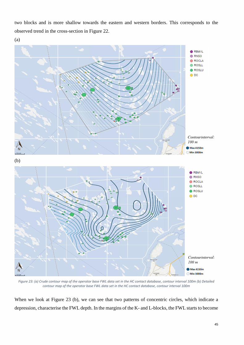
45

two blocks and is more shallow towards the eastern and western borders. This corresponds to the

observed trend in the cross-section in Figure 22.

(a)

(b)

Figure 23: (a) Crude contour map of the operator base FWL data set in the HC contact database, contour interval 100m (b) Detailed contour map of the operator base FWL data set in the HC contact database, contour interval 100m

When we look at Figure 23 (b), we can see that two patterns of concentric circles, which indicate a

depression, characterise the FWL depth. In the margins of the K- and L-blocks, the FWL starts to become

46

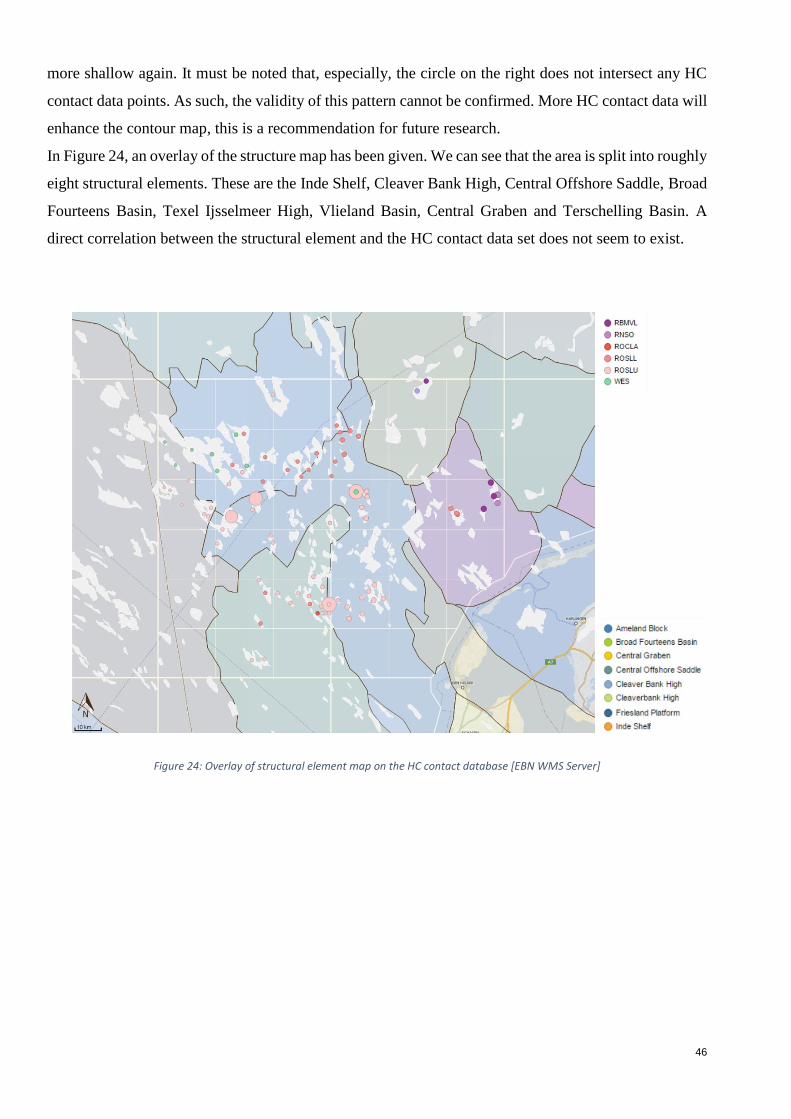
more shallow again. It must be noted that, especially, the circle on the right does not intersect any HC

contact data points. As such, the validity of this pattern cannot be confirmed. More HC contact data will

enhance the contour map, this is a recommendation for future research.

In Figure 24, an overlay of the structure map has been given. We can see that the area is split into roughly

eight structural elements. These are the Inde Shelf, Cleaver Bank High, Central Offshore Saddle, Broad

Fourteens Basin, Texel Ijsselmeer High, Vlieland Basin, Central Graben and Terschelling Basin. A

direct correlation between the structural element and the HC contact data set does not seem to exist.

Figure 24: Overlay of structural element map on the HC contact database [EBN WMS Server]

47

Figure 25: Regional reservoir facies distribution map of the Upper Slochteren Member overlain on the HC contact database, after [ Doornenbal, H., 2010]

Figure 26: Reservoir facies distribution map of the Upper Slochteren Member overlain on the HC contact database, after [Doornenbal, H., 2010]

48

Figure 25 shows an overlay of the Upper Slochteren facies map in the area. Figure 26 is more zoomed

in and shows the two areas in more detail. In Figure 26, we can see that the HC contact data of the Upper

Slochteren Member is split into two zones. To the West it is characterized by playa margin, i.e. coastal

sand belts, in the East it is fluvially dominated. Fluvial-facies types tend to be more cemented and form

poor reservoir zones [Doornenbal, H., 2010]. This means that the difference between the GWC and the

FWL is expected to be larger in the fluvially dominated area because the average pore radius in a more

tightly cemented interval is lower. Using the HC data set, we calculated this difference for both regions

specifically. The average capillary height in the western region was 21.5 m, whereas the average

capillary height in the eastern fluvially dominated area was 29.2 m. As expected, the decrease in reservoir

quality in the eastern area can be observed in the larger capillary height. Furthermore, using equation

(19), we can compute a theoretical capillary rise to see how much the reduced reservoir quality has

impacted the pore throat radius. Assuming that the other variables in the capillary equation, such as

wettability, remain constant, we can see that the pore throat radius decreases by approximately 28.8%.

Figure 27: FWL difference between the optimistic and pessimistic FWL determination of operators

.

49

In Figure 27, an illustration has been given of operator FWL data. As previously analysed in the chapter

Uncertainty Analysis, the position of the FWL cannot be pinpointed with absolute certainty. Instead,

operators use a range of possible FWL contacts based on regional trends and wireline data. The range of

the lowest (i.e. optimistic) FWL height estimation to the highest (i.e. pessimistic) FWL height estimation

of the operator can be used as an indication of the confidence the operator has in the FWL estimation.

In this range is a base (i.e. modus) FWL which the operator deems most likely, and it is this FWL height

which is used for volumetric calculations and further reservoir modelling. In Figure 27, all of the

respective base FWL depths have been adjusted to the same reference level (i.e. 0 m). In this way, the

variation in the FWL range of the different wells can be compared. Although the data set in Figure 27

does not show all of the operator FWL data in the HC database, it does show the huge variance in the

FWL range among the different wells. Using the complete data set, a standard deviation for the FWL

range was calculated as approximately 55 m. Looking at, for instance, the FWL interval in well L07-H-

01, which was approximately 360 m, this is far outside the standard deviation, and it is indicative of a

large uncertainty in the exact height of the FWL.

Further Discussion As demonstrated in the data visualisations, the HC contact database is an incredibly versatile tool which

(in the right hands) can be used for much more than solely a map of HC contact depths in the subsurface.

Using the underlying theorem behind the capillary rise, we can provide estimations about reservoir

characteristics, such as pore throat radii, which can be linked to porosity, permeability and even reservoir

compaction. Furthermore, we have also demonstrated that the HC contact database can be used to

validate the facies distribution in a geological area. However, we assumed that the facies distribution

solely influences the pore throat radii. In reality, the environment of the deposition affects more variables

which also influence the capillary rise. For example, the presence of shale in a reservoir system also

influences the interfacial tension and contact angle. Furthermore, shale also influences the wettability of

the reservoir system, and contact angle measurements do not necessarily represent the true wettability

of shaly systems [Qing, L., et al., 2015].

The same assumption applies for the uncertainty analysis of the capillary rise. In this analysis, the contact

angle was assumed to be between 0° and 45°, which indicate a highly water-wet system. This was done

because in a two-phase gas-water system, it is standard to assume a water-wet system [Zhang, M., et al.,

2016; Hagoort, J., 1988]. However, the work of Zhang showed that the wettability of a two-phase gas-

water system is more nuanced and that both theory and experiments demonstrate that gas wetness cannot

always be overlooked [Zhang, M., et al., 2016].

50

Although this database is an excellent tool for quantifying HC contact depths in the region, it is

insufficient to use for analysing spill points. For analysing reservoir spill points using HC contact data,

an intimate knowledge of the geology and spill point depths of a region (or prospect) is required. It is

insufficient to solely know maximum gas columns and FWLs/GWCs. A significant topic of uncertainty

is the lowest depth of the reservoir. This lowest point in the reservoir structure is critical for spill point

analysis. It is essentially the deepest point in the structure which can trap HCs. For the determination of

this spill point, operator isochoric maps have been used. However, these isochoric maps are the result of

subsurface models, and as such, they are subject to large uncertainties and thus are not suitable to use

for spill point analysis.

In the HC contact database, the vast majority of the reservoirs are represented by one set of FWLs and

GWCs, which are determined based on the exploration well. For smaller reservoirs, this is sufficient.

However, the work of Van Hulten showed that most offshore gas fields have a connected gas volume of

1 − 4 ∙ 109 𝑚3 𝑤𝑒𝑙𝑙⁄ and often a poorly connected compartment which does not communicate

effectively with the well [Van Hulten, F., F., N., 2010]. As a comparison, the Groningen Gas Field has

a connected gas volume of approximately 10 ∙ 109 𝑚3 𝑤𝑒𝑙𝑙⁄ . Depending on the amount of flow

communication between compartments in a specific reservoir, multiple GWCs and FWLs may be

measured within this one reservoir. Therefore, the strength of the HC contact database lies in analysing

regions. For a more detailed look inside reservoirs, a more extensive investigation has to be performed.

Another assumption about the GWCs in the reservoirs is that they are all in equilibrium, i.e. the contacts

are horizontal. Jauhari showed that permeability variations within a reservoir causes lateral height

differences in the transition zone, which can make a GWC appear to be tilted [Jauhari, U., et al., 2012].

Using top of reservoir maps, we have compiled the gas column height of 73 reservoirs. The column

height can be calculated by subtracting the FWL depth from the top of reservoir depth. The column

heights of a reservoir can provide valuable knowledge, the most obvious being volumetrics (providing

we know the net-to-gross). Providing that we also know the spill-point depth than we can also

qualitatively assess whether a reservoir is under-filled. For instance, if we know the that the different

compartments in a compartmentalised reservoir have different gas column heights then this may be an

indication that a sealing fault in a specific compartment is leaking.

51

Recommendations

As mentioned before, the HC contact database is largely populated with regional data, i.e. a single

FWL/GWC data set in each field. A great addition would be if the database could be populated more

with individual well data instead of using solely the exploration well to determine the GWC/FWL.

However, a caveat in populating the database with more wells is that a large number of wells are placed

when the field is already in production. The implication of this is that the HC contacts measured in this

production well will be altered due to pressure depletion. When adding a new well to the database, a

system must be in place to signal that the new FWL/GWC is not comparable to that of the exploration

well. Therefore, the contact data of a well that measured a ‘virgin’ reservoir and data from a well which

measured a mature field have to properly labelled in the HC contact database.

Using the HC database, we can use the difference in the GWC and FWL to deduce a capillary pressure,

which then can be used to compute theoretical porosity and permeability. The TNO porosity and

permeability distribution maps can be used to compare the theoretically derived values of porosity and

permeability when using the GWC/FWL difference. In this way, data can be validated and cross-

checked.

To assess possible HC migration paths, an intimate knowledge of the reservoir structures needs to be

obtained with respect to spill points. The best approach is to concentrate on a small area and to use Petrel

to generate reliable reservoir isochore maps with up-to-date data (at field scale). However, determining

spill points is more nuanced than simply finding the bottom of a trapping structure. Other factors, such

as fault sealing, which can affect HC migration also need to be assessed. Ultimately, using FWL contour

maps with knowledge about the region, i.e. spill points, we can start to look for regions which contain

interesting prospects.

Furthermore, we can use the operator uncertainty (Figure 27) in HC contact depth to correlate this

uncertainty to regions. This way we can investigate whether there are areas in which there is a high

uncertainty in HC contact depth. We can then verify whether these areas of high uncertainty are

geologically more ‘complex’.

52

Conclusions

The HC contact database is the first step in an integrated assessment of the HC prospectivity in an area.

Using data from approximately 122 wells, the K- & L-blocks of offshore Netherlands have been mapped

using operator-sourced data, and a verification using pressure data, quick-look petrophysical analysis

and saturation modelling has been made. The Permian basins form the overwhelming majority of data

with 81% of an Upper or Lower Slochteren Member.

An uncertainty analysis of the Slochteren Formation shows that the pore throat radius is the most

important variable for the capillary height. Using Gaussian error propagation, we can conclude that

global uncertainty 𝛿𝑄 for the wireline height is approximately 12.9 𝑚. When we disregard the

uncertainty of tool sticking, we get 𝛿𝑄 = 4.8 𝑚.

We have seen that the operator standard deviation is approximately 55 m for Slochteren. This result was

obtained by averaging the variances of the data set and calculating a standard deviation for the Slochteren

Formation. The uncertainty in some wells is larger than in others, reflecting the confidence the operator

has in the FWL estimation.

Using data visualisations, we have seen that the reservoirs gradually age from east to west. Triassic

reservoirs are solely present in the easternmost region of the L-block, whereas the oldest Carboniferous

reservoirs are present in the northwestern part of the K-block. The Slochteren Formation also displays a

clear separation, with the Upper Slochteren Member being situated more in the southeastern part and the

Lower Slochteren Member towards the northwestern part of the region.

The HC contact database can be used to validate the compaction of reservoir materials judging by the

change in the capillary height. However, it should be noted that the linear porosity regression line from

Ramm and Bjørlykke against which the results have been compared is purely empirical.

The facies distribution of the Upper Slochteren Member can be verified using the HC contact database.

Assuming that the other variables in the capillary equation remain constant, we can see that the pore

throat radius reduces with approximately 28.8% in the fluvially dominated part of the Upper Slochteren

sandstone compared to the non-fluvially dominated part. This corresponds to the fact that fluvial-facies

types tend to be more cemented and form poor reservoir zones [Doornenbal, H., 2010].

53

Bibliography

[Amorin, R., Broni-Bediako, E., 2010, Application of Minimum Curvature Method to Wellpath

Calculations, Research Journal of Applied Sciences, Engineering and Technology 2(7): 679-686, ISSN:

2040-746]

[Bera, A., Belhadj, H., 2016, A comprehensive review on characterization and modeling of thick

capillary transition zones in carbonate reservoirs, Journal of Unconventional Oil and Gas Resources 16,

Elsevier, pp76-89]

[Cannon, S., 2015, Petrophysics: A Practical Guide, Chapter 7. Petrophysical Workflows, pp115-126,

John Wiley & Sons, Ltd]

[Corona, F., V., 2005, Fault trap analysis of the Permian Rotliegend gas play. Lauwerszee Trough, NE

Netherlands. In: DoRI, A. G. & VINING, B. A. (eds) Petmietan Geologv: North- West Eumpe and

Globat Perspectives. Proceedings of the 6th Petroleum Geology Conference, Geological Society,

London, pp.327—335]

[Craig, F., F., J., 1993, "The Reservoir Engineering Aspect of Waterflooding," S.P.E., vol. 3, H. L.

Doherty Memorial Fund of AIME]

[Doornenbal, H., 2010, Petroleum Geological Atlas of the Southern Permian Basin Area, EAGE

Publications bv]

[Falke, H., 1975, The Continental Permian in Central, West, and South Europe, Proceedings of the

NATO Advanced Study Institute held at the Johannes Gutenberg University, Mainz, Springer Science

& Business Media]

[Fisher, Q., J., 2006, "Fault Sealing Processes in Siliciclastic Sediments," Rock Deformation Research

Group, Leeds]

[Fisher, Q., J., 2001, "The permeability of faults within siliciclastic petroleum reservoirs of the North

Sea and Norwegian Continental Shelf," Elsevier, Leeds]

[Fjaer, E., Holt, R., M., Horsrud, P., Raaen, A., M., Risnes, R., 2008, Petroleum Related Rock

Mechanics, Developments in Petroleum Science 53, Elsevier, pp 437]

[Frikken. H. W. & Stark, J. B. 1993. Character and performance of small Rotliegend gas reservoirs,

Central Offshore Netherlands. In: AASEN, J. 0.. BULLER, A.T., HJELMELAND, 0., HOLT, R. M.,

KLEPPE, J. & TORSJETER. 0. (eds) North Sea Oil and Gas Reservoirs— III, Proceedings of the 3rd

North Sea Oil and Gas Reservoirs Conference. Trondheim. Norway, Kluwer, Dordrecht, 41—50]

[Geluk, M.,C., 2007, Geology of the Netherlands, Edita-the Publishing House of the Royal, Chapter:

Permian, pp 63-83]

[Gerlitz, K., 2004, Implementing the Minimum Curvature Method for Deviated Well Geometry Surveys

in CE7]

[Glennie, K., 1998, "Lower Permian - Rotliegend, Petroleum Geology of the North Sea.," Petroleum

Geology of the North Sea., vol. Blackwell Science, pp. 137-174]

54

[Guapp R. and Okkerman J.A., 2012, Diagenesis and reservoir quality of Rotliegend sandstones in the

northern Netherlands – a review]

[Hall, M., 2012, Do you know what you think you know?, Focus Article, Official publication of the

Canadian Society of Exploration Geophysics, Vol. 37, No. 02]

[Hagoort, J., 1988, Fundamentals of Gas Reservoir Engineering, vol. 23, Elsevier Science]

[Holt, R. M., Lehr, C., Kenter, C. J., & Spits, P., 2003, In-Situ Porosity from Cores: Poroelastic

Correction for Stress Relief during Coring. Society of Petrophysicists and Well-Log Analysts.]

[Horst, F., 1972, Rotliegend: Essays on European Lower Permian, International sedimentary

petrographical series, Brill, 299 pages]

[Hussein, R., A., M., and Ahmed, M., E., B., 2012, Petrophysical Evaluation of Shaly Sand Reservoirs

in Palouge-Fal Oilfield, Melut Basin, South East of Sudan, Journal of Science and Technology Vol. 13,

No.2]

[Jauhari, U., et al., 2012, Hydrodynamic Trapping, Tilted Contacts and New opportunities in Mature

Onshore Kutei Basin, East Kalimantan, Indonesia, Search and Discovery Article #41060, AAPG]

[Knott, S., D., 1993, Fault seal analysis in the North Sea. American Association of Petroleum Geologists

Bulletin. 77, pp 778—792]

[Lo, E, 2005, Gaussian error propagation applied to ecological data, Ecological Monographs, 75(4),

2005, pp. 451-466, Ecological Society of America]

[Mohammadi, S., 2015, Monitoring Wettability Alteration of Poreus Media by Silica Nanoparticles: An

Experimental Approach, Research Institute of Petroleum Industry, Faculty of Research dan

Development of Oil Upstream Indusrty, Tehran]

[Moore, W., R., Zee Ma, Y., Urdea, J., and Bratton, T., 2011, Uncertainty analysis in well-log and

petrophysical interpretations, in Y. Z. Ma and P. R.La Pointe, eds., Uncertainty analysis and reservoir

modeling: AAPG Memoir 96, p. 17 – 28]

[Moradzadeh, A., 2011, Methods of water saturation estimation: Historical Perspective, Journal of

Petroleum and Gas Engineering Vol. 2(3), pp. 45-53]

[Moscariello, A., 2014, The Evolution of the Rotliegend Play in the Permian Basin (NW Europe)

Through Geological Time and Industry Wisdom, Search and Discovery Article #10689]

[Nelson, P.,H., 2009, Pore-throat sizes in sandstones, tight sandstones, and shales, AAPG Bulletin, V.93

no.3, pp 329-340]

[Pham, T., R., et al., "Field Example of Capillary Pressure Effects on Wireline Formation Tester

Measurements and OWC Estimation in a Mixed-Wettability Oil Reservoir," SPE, p. 14, 2005]

[Qing, L., et al., 2015, A comparative investigation of shale wettability: The significance of pore

connectivity, Journal of Natural Gas Science and Engineering, Volume 27, pp 1174-1188]

[Ramm, M., Bjørlykke, K., 1994, Porosity/Depth Trends In Reservoir Sandstones, Norsk Hydro,

University of Oslo]

55

[Rider, M., H., 1996, The Geological Interpretation of Well Logs, Sutherland: Rider-French Consulting

Ltd.]

[Rondeel, H., E., et al, 1996, Geology of Gas and Oil under the Netherlands: Selection of papers

presented at the 1993 International Conference of the American Association of Petroleum Geologists,

held in The Hague, Springer Science & Business Media, 284 pages]

[Rushing, J., A., Newsham, K.,E., Van Fraassen, K.,C., 2008, Laboratory Measurements of Gas-Water

Interfacial Tension at HP/HT Reservoir Conditions, SPE 114516]

[Spearing, M.C., Abdou, M., Azagbaesuweli, G., Kalam, M.Z., 2014, Transition zone behavior: The

measurement of bounding and scanning relative permeability and capillary pressure curves at reservoir

conditions for a giant carbonate reservoir, SPE-171892-MS]

[Staube, A., J., & Milius, G., 1970, Geology of Groningen Gas field, Netherlands, Mem. Amer. Assoc.

Petroleum Geol., 14, pp 359-369]

[Teeuw, D., 1971, Prediction of formation compaction from laboratory compressibility data. “Society

of Petroleum Engineers”, Journal 11, pp. 263-271]

[Thulin, K., Li, G., Aanonsen, S., I., Reynolds, A., C., 2007, Estimation of Initial Fluid Contacts by

Assimilation of Production Data With EnKF, SPE 109975]

[Wong. T. E.. Batjes, D. A. J. & De Jager, J., 2007. Geologv of the Netherlands. Royal Netherlands

Academy of Arts and Sciences, Amsterdam. 354]

[Woodhouse, R. and Warner, H.R., 2005, Sw and Hydrocarbon Pore Volume Estimates in Shaly Sands

- Routine Oil-Based-Mud Core Measurements Compared With Several Log Analysis Models. Presented

at the SPE Annual Technical Conference and Exhibition, Dallas, Texas, 9-12 October 2005. SPE-96618-

MS]

[Van Der Molen, 1.. Zijlstra, E. B., Okkerman. J. A. & Reemst, P. H. M. 2003. Compartmentalisation

in Rotliegend gas fields, examples from offshore and onshore the Netherlands. In: KONSTANTY, J. J.

C., GRAULS, D. & GELDER. E. N. (conv). Fault and Top Sea/s: What do we know and where do we

go? European Association of Geoscientists and Engineers, Montpellier, Paper-28]

[Van Hulten, F., F., N., 2010, Geological factors effecting compartmentalization of Rotliegend gas fields

in the Netherlands, Geological Society, London, Special Publications, V. 347, pp 301-315]

[Van Wijhe. D. H., Lutz, M. & Kaasschieter, J. P. H., 1980, The Rotliegend in the Netherlands and its

gas accumulations. Geologie en Mijnbouw, 59, 3—24]

[Zhang, M., et al., 2016, "Quantitative measurement of gas wettability of different substrates," Energy

Sources, Part A: Recovery, Utilization, and Environmental Effects, vol. 38, no. 4]

[Zijlstra, E. 8., Reemst. P. H. M. & Fisher, Q. J. 2007. Incorporation of fault properties into production

simulation models of Permian reservoirs from the southern North Sea. In: ]OLLEY, S. J., BARR. D.,

WALSH, J. J. & KNIPE. R. J. (eds) Structural Complex Reservoirs. Geological Society, London, Special

Publication, 292. 295—308]