From random walk trajectories to random interlacementscerny/publications/ebp.pdf · random walk represents a corrosive particle wandering erratically through 1. 2 Cern y, Teixeira

ENSAIOS MATEMATICOS

200X, Volume XX, X–XX

From random walk trajectories

to random interlacements

Jirı CernyAugusto Teixeira

Abstract. We review and comment recent research on random inter-lacements model introduced by A.-S. Sznitman in [43]. A particular em-phasis is put on motivating the definition of the model via natural questionsconcerning geometrical/percolative properties of random walk trajectorieson finite graphs, as well as on presenting some important techniques usedin random interlacements’ literature in the most accessible way. This textis an expanded version of the lecture notes for the mini-course given at theXV Brazilian School of Probability in 2011.

2000 Mathematics Subject Classification: 60G50, 60K35, 82C41, 05C80.

Acknowledgments

This survey article is based on the lecture notes for the mini-course onrandom interlacements offered at the XV Brazilian School of Probability,from 31st July to 6th August 2011. We would like to thank the organizersand sponsors of the conference for providing such opportunity, speciallyClaudio Landim for the invitation. We are grateful to David Windischfor simplifying several of the arguments in these notes and to A. Drewitz,R. Misturini, B. Gois and G. Montes de Oca for reviewing earlier versionsthe text.

Contents

1 Introduction 1

2 Random walk on the torus 72.1 Notation . . . . . . . . . . . . . . . . . . . . . . . . . . . . . 72.2 Local entrance point . . . . . . . . . . . . . . . . . . . . . . 92.3 Local measure . . . . . . . . . . . . . . . . . . . . . . . . . . 132.4 Local picture as Poisson point process . . . . . . . . . . . . 162.5 Notes . . . . . . . . . . . . . . . . . . . . . . . . . . . . . . 17

2.5.1 Disconnection of a discrete cylinder . . . . . . . . . 18

3 Definition of random interlacements 203.1 Notes . . . . . . . . . . . . . . . . . . . . . . . . . . . . . . 26

4 Properties of random interlacements 274.1 Basic properties . . . . . . . . . . . . . . . . . . . . . . . . . 274.2 Translation invariance and ergodicity . . . . . . . . . . . . . 294.3 Comparison with Bernoulli percolation . . . . . . . . . . . . 324.4 Notes . . . . . . . . . . . . . . . . . . . . . . . . . . . . . . 36

5 Renormalization 375.1 Notes . . . . . . . . . . . . . . . . . . . . . . . . . . . . . . 41

6 Interlacement set 436.1 Notes . . . . . . . . . . . . . . . . . . . . . . . . . . . . . . 50

7 Locally tree-like graphs 527.1 Random interlacements on trees . . . . . . . . . . . . . . . . 527.2 Random walk on tree-like graphs . . . . . . . . . . . . . . . 55

7.2.1 Very short introduction to random graphs . . . . . . 577.2.2 Distribution of the vacant set . . . . . . . . . . . . . 587.2.3 Random graphs with a given degree sequence. . . . . 597.2.4 The degree sequence of the vacant graph . . . . . . . 60

7.3 Notes . . . . . . . . . . . . . . . . . . . . . . . . . . . . . . 61

CONTENTS

Index 63

Bibliography 65

Chapter 1

Introduction

These notes are based on the mini-course offered at the ‘XV BrazilianSchool of Probability’ in Mambucaba in August 2011. The lectures tried tointroduce the audience to random interlacements, a ‘dependent-percolation’model recently introduced by A.-S. Sznitman in [43]. The emphasis wasput on motivating the definition of this model via some natural questionsabout random walks on finite graphs, explaining the difficulties that appearwhen studying the model, and presenting some of the techniques used toanalyze random interlacements. We tried to present these techniques inthe simplest possible way, sometimes at expense of generality.

Let us start setting the stage for this review by introducing one of theproblems which motivated the definition of random interlacements. To thisend, fix a finite graph G = (V, E) with a vertex set V and an edge set E ,and denote by (Xn)n≥0 a simple random walk on this graph, that is theMarkovian movement of a particle on G prescribed as follows: It starts ata given (possibly random) vertex x ∈ G, X0 = x, and given the positionat time k ≥ 0, say Xk = y, its position Xk+1 at time k + 1 is uniformlychosen among all neighbors of y in G.

Random walks on finite and infinite graphs, in particular on Zd, hasbeen subject of intense research for a long time. Currently, there is a greatdeal of studying material on this subject, see for instance the monographs[26, 27, 28, 38, 54]. Nevertheless, there are still many interesting questionsand vast areas of research which are still to be further explored.

The question that will be of our principal interest was originally askedby M.J. Hilhorst, who proposed the random walk as a toy model for cor-rosion of materials. For sake of concreteness, take the graph G to be thed-dimensional discrete torus TdN = (Z/NZ)d which for d = 3 can be re-garded as a piece of crystalline solid. The torus is made into a graphby adding edges between two points at Euclidean distance one from eachother. Consider now a simple random walk (Xn)n≥0, and imagine that thisrandom walk represents a corrosive particle wandering erratically through

1

2 Cerny, Teixeira

the crystal, while it marks all visited vertices as ‘corroded’. (The particlecan revisit corroded vertices, so its dynamics is Markovian, i.e. it is notinfluenced by its past.)

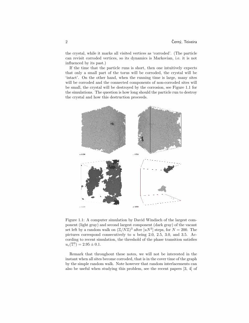
If the time that the particle runs is short, then one intuitively expectsthat only a small part of the torus will be corroded, the crystal will be‘intact’. On the other hand, when the running time is large, many siteswill be corroded and the connected components of non-corroded sites willbe small, the crystal will be destroyed by the corrosion, see Figure 1.1 forthe simulations. The question is how long should the particle run to destroythe crystal and how this destruction proceeds.

Figure 1.1: A computer simulation by David Windisch of the largest com-ponent (light gray) and second largest component (dark gray) of the vacantset left by a random walk on (Z/NZ)3 after [uN3] steps, for N = 200. Thepictures correspond consecutively to u being 2.0, 2.5, 3.0, and 3.5. Ac-cording to recent simulation, the threshold of the phase transition satisfiesuc(T3

· ) = 2.95± 0.1.

Remark that throughout these notes, we will not be interested in theinstant when all sites become corroded, that is in the cover time of the graphby the simple random walk. Note however that random interlacements canalso be useful when studying this problem, see the recent papers [3, 4] of

Random Walks and Random Interlacements 3

D. Belius.In a more mathematical language, let us define the vacant set left by the

random walk on the torus up to time n

VN (n) = TdN \ X0, X1, . . . , Xn. (1.1)

VN (n) is the set of non-visited sites at time n (or simply the set non-corroded sites at this time). We are interested in connectivity properties ofthe vacant set, in particular in the size of its largest connected component.

We will see later that the right way to scale n with N is n = uNd foru ≥ 0 fixed. In this scaling the density of the vacant set is asymptoticallyconstant and non-trivial, that is is for every x ∈ TdN ,

limN→∞

Prob[x ∈ VN (uNd)] = c(u, d) ∈ (0, 1). (1.2)

This statement suggest to view our problem from a slightly differentperspective: as a specific site percolation model on the torus with density(roughly) c(u, d), but with spatial correlations. These correlations decayrather slowly with the distance, which makes the understanding of themodel delicate.

At this point it is useful to recall some properties of the usual Bernoullisite percolation on the torus TdN , d ≥ 2, that is of the model where the sitesare declared open (non-corroded) and closed (corroded) independently withrespective probabilities p and 1−p. This model exhibits a phase transitionat a critical value pc ∈ (0, 1). More precisely, when p < pc, the largestconnected open cluster C?max(p) is small with high probability,

p < pc =⇒ limN→∞

Prob[|C?max(p)| = O(logλN)] = 1, (1.3)

and when p > pc, the largest connected open cluster is comparable withthe whole graph (it is then called giant),

p > pc =⇒ limN→∞

Prob[|C?max(p)| ∼ Nd] = 1. (1.4)

Much more is known about this phase transition, at least when d is large[9, 10]. A similar phase transition occurs on other (sequences of) finitegraphs, in particular on large complete graph, where it was discovered (forthe edge percolation) in the celebrated paper of Erdos and Renyi [18].

Coming back to our random walk problem, we may now refine our ques-tions: Does a similar phase transition occur there. Is there a critical valueuc = uc(Td· ) such that, using Cmax(u,N) to denote the largest connectedcomponent of the vacant set on TdN at time uNd,

u < uc =⇒ limN→∞

Prob[|Cmax(u,N)| ∼ Nd] = 1,

u > uc =⇒ limN→∞

Prob[|Cmax(u,N)| = o(Nd)] = 1 ?(1.5)

4 Cerny, Teixeira

At the time of writing of these notes, we have only partial answers toto this question (see Chapter 2 below). It is however believed that thisphase transition occurs for the torus in any dimension d ≥ 3. This beliefis supported by simulations, cf. Figure 1.1.

Remark 1.1. It is straightforward to see that such phase transition does notoccur for d ∈ 1, 2. When d = 1, the vacant set at time n is a segment oflength roughly (N − (n1/2ξ))∨ 0, where ξ is a random variable distributedas the size of the range of a Brownian motion at time 1. Therefore, thescaling n = uNd = uN in (1.2) is not interesting. More importantly, itfollows from this fact that no sharp phase transition occurs even on the‘corrected’ scaling, n = uN2. The situation in d = 2 is more complicated,but the fragmentation is qualitatively different from the case d ≥ 3.

The phase transition for the Bernoulli percolation on the torus, (1.3),(1.4), can be deduced straightforwardly from the properties of its ‘infinitevolume limit’, that is the Bernoulli percolation on Zd which is very wellunderstood (see e.g. the monographs [19, 8]). It is thus legitimate to askwhether there is an infinite volume percolation which is a local limit of thevacant set. This question is not only of theoretical interest, there are manyproblems that are easier to solve in the infinite volume situation. As wewill see, the existence of the phase transition is one of them.

One of the main goals of these notes is to construct explicitly this in-finite volume limit, which is called random interlacements, and study itsproperties. We will not go into details how these properties can be thenused to control the finite volume problem, even if not surprisingly, therecent progress in understanding random interlacements has been usefulto analyze the original questions concerning the vacant set on the torus,see [49].

Organization of these notes

In the first chapters of these notes we restrict our analysis to d-dimensionaltorus and Zd, with d ≥ 3, cf. Remark 1.1.

In Chapter 2, we study the random walk on the torus, aiming on moti-vating the construction of random interlacements. We will define what wecall the ‘local-picture’ left by the random walk on TdN . To be more precise,suppose that N is large and that we are only interested in what happens ina small fixed box A ⊂ TdN . It is clear that as the number of steps n of thewalk grows, the random walk will visit A several times, leaving a ‘texture’of visited and non-visited sites inside this box.

To control this texture we split the random walk trajectory into whatwe call ‘excursions’ which correspond to the successive visits to A. Usingsome classical results from random walk theory, we will establish three keyfacts about these excursions:


(i) the successive excursions to A are roughly independent from eachother,

(ii) the first point in A visited by each excursion has a limiting distribu-tion (as N grows), which we call the normalized equilibrium distri-bution on A.

(iii) when the number of steps n scales as uNd, the number of excursionsentering A is approximately Poisson distributed (with parameter isproportional to u).

All these properties hold precisely in the limit N → ∞ when A is keptfixed.

Starting from these three properties of the random walk excursions, wedefine a measure on 0, 1A, which is the candidate for the asymptoticdistribution of the wanted infinite volume percolation (intersected with A).This limiting distribution is what we call the local picture. In view ofproperties (i)–(iii), it should not be surprising that Poisson point processesenter the construction here.

In Chapter 3, we will use this local picture to give a definition of randominterlacements. To this end we map A ⊂ TdN into its isometric copy A ⊂Zd and transfer the local picture to 0, 1A. Then, taking the limit as

A ↑ Zd, we essentially obtain a consistent measure on 0, 1Zd , which wecall random interlacements.

The actual construction of random interlacements given in Chapter 3is more complicated, because its goal is not only to prove the existence(and uniqueness) of the infinite volume measure, but also to provide away to perform calculations. In particular, the actual construction aimson preserving the Poisson point process structure appearing in the localpicture.

We will construct the random interlacements as a trace left on Zd bya Poisson point process on the space of doubly infinite random walk tra-jectories modulo time shift, see (3.10) below. Intuitively speaking, everytrajectory appearing in this Poisson point process correspond to one ex-cursion of the random walk in the torus.

In Chapter 4, after having defined the random interlacements measure,we will describe some of its basic properties. We will study its correlations,translation invariance and ergodicity, and compare it to Bernoulli site per-colation. This comparison helps determining which of the techniques thathave already been developed for Bernoulli percolation have chance to workin the random interlacements setting.

As we will find out, many of the techniques of Bernoulli percolation arenot directly applicable for random interlacements. Therefore, we will needto adapt them, or develop new techniques that are robust enough to deal

6 Cerny, Teixeira

with dependence. In Chapter 5, we prove a result related to the existenceof a phase transition for random interlacements on high dimensions, seeTheorem 5.1. The proof of this theorem makes use of a technique which isvery important in various contexts, namely the multi-scale renormalization.

The last two chapters of these notes present two recent branches of therandom interlacements research. In Chapter 6, we study the propertiesof the interlacement set of random interlacements on Zd. This set is thecomplement of the vacant set, and should be viewed as the limit of occu-pied/corroded sites in the random-walk-on-torus problem. We will see thatthe properties of the interlacement set are rather well understood, contraryto those of the vacant set.

Finally, in Chapter 7, we return to random walk on finite graphs, thistime however not on the torus, but on random regular graphs. We explainthat the infinite volume limit of this problem is random interlacements onregular trees, and sketch the techniques used to show that for these graphsthere is a phase transition in the spirit of (1.5).

We would like to precise the scope and structure of these notes. We donot want to present a comprehensive reference of what is currently knownabout random interlacements. Instead, we intend to favor a motivatedand self-contained exposition, with more detailed proofs of basic facts thatshould give the reader familiarity with the tools needed to work on thesubject. The results presented here are not the most precise currentlyavailable, instead they were chosen in a way to balance between simplicityand relevance. For interested reader we collect the pointers to the relevantliterature at the end of each chapter.

Chapter 2

Random walk on the torus

In this chapter we discuss some properties of random walk on a discretetorus. Our aim is to motivate the definition of the local picture discussedin the Introduction, that is to understand the intersection of the trajectoryof the random walk with a fixed set A ⊂ TdN as N becomes large.

2.1 Notation

Let us start by fixing the notation used through these notes. We consider,for N ≥ 1, the discrete torus TdN = (Z/NZ)d, which we regard as a graphwith an edge connecting two vertices if and only if their Euclidean distanceis one.

On TdN we consider a simple random walk. For technical reasons thatwill be explained later, we actually consider the so called lazy randomwalk which stays put, with probability one half, and jumps otherwise to auniformly chosen neighbor. Its transition matrix is given by

C(x, y) =

1/2, if x = y,

1/(4d), if x and y are neighbors in TdN ,

0, otherwise.

(2.1)

Let π be the uniform distribution on the torus TdN . It is easy to see thatπ and C(x, y) satisfy the detailed balance condition, that is π is reversiblefor the random walk.

We write P for the law on (TdN )N of lazy simple random walk on TdNstarted with uniform distribution π. We let Xn, n ≥ 0, stand for thecanonical process on (TdN )N. The law of the canonical (lazy) random walkstarted at a specified point x ∈ TdN is denoted by Px.

Note that we omit the dependence on N in the notation π, P , Px andXn. This will be done in other situations throughout the text, hoping thatthe context will clarify the omission.

7

8 Cerny, Teixeira

For k ≥ 0, we introduce the canonical shift operator θk in the space oftrajectories (TdN )N, which is characterized by Xn θk = Xn+k for everyn ≥ 0. Analogously, we can define θT for a random time T .

The main reason for considering the lazy random walk are the followingfacts:

C(·, ·) has only positive eigenvalues 1 = λ1 > λ2 ≥ · · · ≥ λNd ≥ 0. (2.2)

The spectral gap ΛN := λ1 − λ2 satisfies ΛN ≥ cN−2, (2.3)

see for instance [28], Theorems 5.5 and 12.4. A simple calculation usingthe spectral decomposition leads then to

supx,y∈TdN

∣∣Px[Xn = y]− π(y)∣∣ ≤ ce−ΛNn, for all n ≥ 0, (2.4)

see [28], (4.22), (4.35) and Theorem 5.5.It will be useful to define the regeneration time rN associated to the

simple random walk on TdN by

rN = Λ−1N log2N ∼ cN2 log2N. (2.5)

To justify the name regeneration time, observe that, for every x ∈ TdN , by(2.2) and (2.4), the total variation distance between Px[XrN ∈ ·] and πsatisfies

‖Px[XrN ∈ ·]− π(·)‖TV :=1

2

∑y∈TdN

∣∣Px[XrN = y]− π(y)∣∣

≤ c′Nde−c log2N

≤ c′e−c log2N ,

(2.6)

which decays with N faster than any polynomial. This means that, inde-pendently of its starting distribution, the distribution of the random walkposition at time rN is very close to being uniform.

We also consider the simple (lazy) random walk on the infinite latticeZd where edges again connect points with Euclidean distance one. Thecanonical law of this random walk starting at some point x ∈ Zd is denoted

by PZdx . If no confusion may arise, we write simply Px.

We introduce the entrance and hitting times HA and HA of a set A ofvertices in TdN (or in Zd) by

HA = inft ≥ 0 : Xt ∈ A,HA = inft ≥ 1 : Xt ∈ A.

(2.7)

Throughout these notes, we will suppose that the dimension d is greateror equal to three (cf. Remark 1.1), implying that

the random walk on Zd is transient. (2.8)


Fix now a finite set A ⊂ Zd (usually we will denote subsets of Zd byA,B, . . . ). Due to the transience of the random walk, we can define theequilibrium measure, eA, and the capacity, cap(A), of A by

eA(x) := 1x∈APZdx [HA =∞], x ∈ Zd,

cap(A) := eA(A) = eA(Zd).(2.9)

Note that cap(A) normalizes the measure eA into a probability distribution.Throughout this notes we use B(x, r) to denote the closed ball centered

at x with radius r (in the graph distance), considered as a subset of Zd orTdN , depending on the context.

2.2 Local entrance point

We now start the study of the local picture left by the random walk onTdN . To this end, consider a (finite) box A ⊂ Zd centered at the origin.For each N larger than the diameter of A, one can find a copy AN of thisbox inside TdN . We are interested in the distribution of the intersection ofthe random walk trajectory (run up to time n) with the set AN , that isX0, X1, . . . , Xn ∩ AN . As N increases, the boxes AN get much smallercompared to the whole torus TdN , explaining the use of the terminology‘local picture’. In particular, it is easy to see that

π(AN )→ 0 as N →∞. (2.10)

As soon as N is strictly larger than the diameter of the box A, we canfind an isomorphism φN : AN → A between the box AN and its copy A inthe infinite lattice. As usual, to avoid a clumsy notation, we will drop theindices N by φN and AN .

The first question we attempt to answer concerns the distribution of thepoint where the random walk typically enters the box A. Our goal is toshow that this distribution almost does not depend on the starting pointof the walk, if it starts far enough from the box A.

To specify what we mean by ‘far enough from A’, we consider a sequenceof boxes A′N centered at the origin in Zd and having diameter N1/2 (thespecific value 1/2 is not particularly important, any value strictly betweenzero and one would work for our purposes here). Note that for N largeenough A′N contains A and N1/2 ≤ N . Therefore, we can extend theisomorphism φ defined above to φ : A′N → A′N ⊂ Zd, where A′N is a copyof A′N inside TdN . Also π(A′N ) → 0 as N → ∞, therefore, under P , therandom walk typically starts outside of A′N .

The first step in determination of the entrance distribution to A is thefollowing lemma which roughly states that the random walk likely regen-erates before hitting A.

10 Cerny, Teixeira

Lemma 2.1. (d ≥ 3) For A′ and A′ as above, there exists δ > 0 such that

supx∈TdN\A′

Px[HA ≤ rN ] ≤ N−δ, ‘A isn’t hit before regenerating’ (2.11)

supx∈Zd\A′N

PZdx [HA <∞] ≤ N−δ, ‘escape to infinity before hitting A’ (2.12)

Proof. From [26, Proposition 1.5.10] it can be easily deduced that there isc <∞ such that for any ` ≥ 1 and x ∈ Zd, with |x| > `,

PZdx [HB(0,`) <∞] ≤ c

( `

|x|

)d−2

. (2.13)

The estimate (2.12) then follows directly from (2.13).To show (2.11), let Π be the canonical projection from Zd onto TdN .

Given an x in TdN \A′, we can bound Px [HA ≤ rN ] from above by

PZdφ(x)

[HB(φ(x),N log2N)c ≤ rN

]+ PZd

φ(x)

[HΠ−1(A)∩B(φ(x),N log2N) <∞

].

(2.14)

Using (3.30) on p.227 of [29], we obtain

PZdφ(x)

[HB(φ(x),N log2N)c ≤ rN

]≤ PZd

φ(x)

[max

1≤t≤rN|Xt − φ(x)|∞ ≥ cN log2N

]≤ 2d exp−2(cN log2N)2/4rN

≤ ce−c log2N .

(2.15)

The set Π−1(A) ∩ B(φ(x), N log2N) is contained in a union of no morethan c logcN translated copies of the set A. By the choice of x, φ(x) is atdistance at least cN1/2 from each of these copies. Hence, using the unionbound and (2.13) again, we obtain that

Pφ(x)

[HΠ−1(A)∩B(φ(x),N log2N) <∞

]≤ c(logN)cN−c. (2.16)

Inserting the last two estimates into (2.14), we have shown (2.11).

As a consequence of (2.11), we can now show that, up to a typicallysmall error, the probability Py[XHA = x] does not depend much on thestarting point y ∈ TdN \A′:

Lemma 2.2.

supx∈A,

y,y′∈TdN\A′

∣∣∣Py[XHA = x]− Py′ [XHA = x]∣∣∣ ≤ cN−δ. (2.17)


Proof. We apply the following intuitive argument: by the previous lemma,it is unlikely that the random walk started at y ∈ TdN \ A′ visits the setA before time rN , and at time rN the distribution of the random walk isalready close to uniform, i.e. it is independent of y. Therefore the hittingdistribution cannot depend on y too much.

To make this intuition into a proof, we first observe that (2.17) is impliedby

supy∈TdN\A′

∣∣∣Py[XHA = x]− P [XHA = x]∣∣∣ ≤ cN−δ. (2.18)

To show (2.18), we first deduce from inequality (2.4) that

supy∈TdN\A′

∣∣∣Ey[PXrN [XHA = x]]− P [XHA = x]

∣∣∣≤∑y′∈TdN

supy∈TdN\A′

∣∣∣Py[XrN = y′]− π(y′)∣∣∣Py′ [XHA = x]

≤ cNde−c log2N ≤ e−c log2N .

(2.19)

For any y ∈ TdN \ A′, by the simple Markov property applied at time rNand the estimate (2.19),

Py[XHA = x] ≤ Py[XHA = x,HA > rN ] + Py[HA ≤ rN ]

≤ Ey[PXrN [XHA = x]

]+ Py[HA ≤ rN ]

≤ P [XHA = x] + e−c log2N + Py[HA ≤ rN ].

(2.20)

With (2.11), we have therefore shown that for any y ∈ TdN \A′,

Py[XHA = x]− P [XHA = x] ≤ N−δ. (2.21)

On the other hand, for any y ∈ TdN \A′, by the simple Markov property attime rN again,

Py[XHA = x] ≥ Py[XHA = x,HA > rN ]

≥ Ey[PXrN [XHA = x]

]− Py[HA ≤ rN ]

≥ P [XHA = x]−N−δ,(2.22)

using (2.19), (2.11) in the last inequality. Combining (2.21) and (2.22),(2.18) follows.

Given that the distribution of the entrance point of the random walkin A is roughly independent of the starting point (given that the startingpoint is not in A′), we are naturally tempted to determine such distribution.This is the content of the next lemma, which will play an important rolein motivating the definition of random interlacements later.

12 Cerny, Teixeira

Lemma 2.3. For A and A′ as above there is δ > 0 such that

supx∈A, y∈TdN\A′

∣∣∣∣Py[XHA = x]− eA(φ(x))

cap(A)

∣∣∣∣ ≤ N−δ. (2.23)

Note that the entrance law is approximated by the (normalized) exit dis-tribution, cf. definition (2.9) of the equilibrium measure. This is intimatelyrelated to the reversibility of the random walk.

Proof. Let us fix vertices x ∈ A, y ∈ TdN \A′. We first define the equilibriummeasure of A, with respect to the random walk killed when exiting A′,

eA′

A (z) = 1A(z)Pz[HTdN\A′ < HA], for any z ∈ A. (2.24)

Note that by (2.12) and the strong Markov property applied at HTdN\A′ ,

eA(φ(z)) ≤ eA′

A (z) ≤ eA(φ(z)) +N−δ, for any z ∈ A. (2.25)

In order to make the expression Py[XHA = x] appear, we consider theprobability that the random walk started at x escapes from A to TdN \ A′and then returns to the set A at some point other than x. By reversibilityof the random walk with respect to the measure (πz)z∈TdN , we have∑z∈A\x

πxPx[HTdN\A′ < HA, XHA= z] = πxPx[HTdN\A′ < HA, XHA

6= x]

=∑

z∈A\xπzPz[HTdN\A′ < HA, XHA

= x].

(2.26)

By the strong Markov property applied at time HTdN\A′ , we have for anyz ∈ A,

πzPz[HTdN\A′ < HA, XHA= x]

= πzEz

[1HTd

N\A′<HA

PXHTdN\A′

[XHA = x]].

(2.27)

With (2.25) and (2.17), this yields∣∣∣πzPz[HTdN\A′ < HA, XHA= x]−πxeA(φ(z))Py[XHA = x]

∣∣∣ ≤ N−δ, (2.28)

for any z ∈ A. With this estimate applied to both sides of (2.26), we obtain

πxeA(φ(x))(1− Py[XHA = x]

)=Py[XHA = x]

(πx cap(A)− πxeA(φ(x))

)+O

(|A|N−δ

),

(2.29)

implying (2.23).

We observe that the entrance distribution Py[XHB = ·] was approxi-mated in Lemma 2.3 by a quantity that is independent of N and solelyrelates to the infinite lattice random walk. This is a very important ingre-dient of the local picture construction.


2.3 Local measure

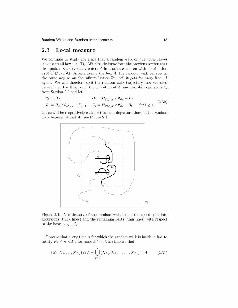
We continue to study the trace that a random walk on the torus leavesinside a small box A ⊂ TdN . We already know from the previous section thatthe random walk typically enters A in a point x chosen with distributioneA(φ(x))/ cap(A). After entering the box A, the random walk behaves inthe same way as on the infinite lattice Zd until it gets far away from Aagain. We will therefore split the random walk trajectory into so-calledexcursions. For this, recall the definition of A′ and the shift operators θkfrom Section 2.2 and let

R0 = HA, D0 = HTdN\A′ θR0+R0,

Rl = HA θDl−1+Dl−1, Dl = HTdN\A′ θRl +Rl, for l ≥ 1.

(2.30)

These will be respectively called return and departure times of the randomwalk between A and A′, see Figure 2.1.

AN

A′N

TdN

X0

R0

D0

R1

D1

Figure 2.1: A trajectory of the random walk inside the torus split intoexcursions (thick lines) and the remaining parts (thin lines) with respectto the boxes AN , A′N .

Observe that every time n for which the random walk is inside A has tosatisfy Rk ≤ n < Dk for some k ≥ 0. This implies that

X0, X1, . . . , XDk ∩A =

k⋃j=0

XRj , XRj+1, . . . , XDj ∩A. (2.31)

14 Cerny, Teixeira

Or in other words, the trace left by the random walk trajectory in A up totime Dk is given by union of the traces of k separate excursions.

Since XDk /∈ A′N , using Lemma 2.2 and the strong Markov propertyapplied at the time Dk, we can conclude that the set of points in A visitedby the random walk between times Rk+1 and Dk+1 is roughly indepen-dent of what happened before the time Dk. Therefore, the excursionsXRj , XRj+1, . . . , XDj, j = 0, 1, 2, . . . , should be roughly independent. Afixed number of such excursions should actually become i.i.d. in the limitN →∞.

Lemma 2.3 yields that the entrance points XRj of these trajectoriesin A are asymptotically distributed as eA(φ(·))/ cap(A). Moreover, as Ngrows, the difference Dk−Rk tends to infinity. Therefore, as N grows, theexcursion XRj+1, . . . , XDj looks more and more like a simple randomwalk trajectory on Zd (note that this heuristic claim is only true becausethe random walk on Zd, for d ≥ 3, is transient).

From the previous arguments it follows that the asymptotic distributionof every excursion should be given by

QA[X0 = x, (Xn)n≥0 ∈ · ] =eA(x)

cap(A)PZdx [ · ], for x ∈ Zd. (2.32)

To understand fully thy trace left by random walk in A, we now have tounderstand how many excursions are typically performed by the randomwalk between A and A′ until some fixed time n.

Using a reversibility argument again, we first compute the expected num-ber of excursions before time n. To this end fix k ≥ 0 and a and let usestimate the probability that k is a return time Rj for some j ≥ 0. Thisprobability can be written as

P [k = Rj for some j ≥ 0]

=∑x∈A

∑y∈(A′)c

∑m≤k

P[Xm = y,Xk = x,Xi ∈ A′ \A,m < i < k

]. (2.33)

Let Γj(y, x) be the set of possible random walk trajectories of length j join-ing y to x and staying in A′ \A between times 1 and j−1. By reversibility,for every γ ∈ Γj(y, x) and l ≥ 0,

P [(Xl, . . . , Xl+j) = γ] = π(y)Py[(X0, . . . , Xj) = γ]

= π(x)Px[(X0, . . . , Xj) = γ],(2.34)

where γ ∈ Γj(x, y) is the time-reversed path γ. Observing that the timereversal is a bijection from Γj(y, x) to Γj(x, y), the right-hand side of (2.33)


can be written as

k∑m=0

∑x∈A

∑y∈(A′)c

∑γ∈Γk−m(y,x)

P [(Xm, . . . , Xk) = γ]

(2.34)=

k∑m=0

∑x∈A

∑y∈(A′)c

∑γ∈Γk−m(x,y)

π(x)Px[(X0, . . . , Xk−m) = γ]

=∑x∈A

k∑m=0

N−dPx[k −m = HTdN\A′ < HA]

= N−d∑x∈A

Px[HTdN\A′ < mink, HA].

(2.35)

We now use (2.25) to obtain that

limN→∞

limk→∞

∣∣∣NdP[k = Rj for some j ≥ 0

]− cap A

∣∣∣ = 0. (2.36)

As the random variables (Ri+1−Ri)i≥0 are i.i.d., the renewal theory yields

limN→∞

N−dE[Ri+1 −Ri] = (cap A)−1. (2.37)

and thus, for all u > 0 fixed,

limN→∞

E[# excursions between times 0 and uNd

]= u cap A. (2.38)

Remark, that we finally obtained a justification for the scaling mentionedin (1.2)!

The expectation of the difference Ri+1 − Ri ∼ Nd is much larger thanthe regeneration time. Hence, typically the random walk regenerates manytimes before returning to A. It is thus plausible that, asymptotically asN → ∞, N−d(Ri+1 − Ri)/ cap A has exponential distribution with pa-rameter 1, and that the number of excursions before uNd has Poissondistribution with parameter cap A. This heuristic can be made rigorous,see [1, 2].

Combining the discussion of the previous paragraph with the asymptotici.i.d. property of the excursions, and with (2.32), we deduce the followingsomewhat informal description of how the random walk visits A:

• the random walk trajectory is split into roughly independent excur-sions,

• for each x ∈ A, the number of excursions starting at x is approxi-mately an independent Poisson random variable with mean ueA(x),

• the trace left by the random walk on A is given by the union of allthese excursions intersected with A.

16 Cerny, Teixeira

To make the last point slightly more precise, observe that with highprobability X0, XuNd /∈ A′, that the times 0 and uNd are not in anyexcursion. So with hight probability there are no incomplete excursion inA at time uNd.

2.4 Local picture as Poisson point process

We are now going to make the above informal construction precise, usingthe formalism of Poisson point processes. For this, let us first introducesome notation. Let W+ be the space of infinite random walk trajectoriesthat spend only a finite time in finite sets of Zd.

W+ =w : N→ Zd : ‖w(n)− w(n+ 1)‖1 ≤ 1 for each n ≥ 0

and n : w(n) = y is finite for all y ∈ Zd.

(2.39)

(Recall that we consider lazy random walk.) As usual, Xn, n ≥ 0, denotethe canonical coordinates on W+ defined by Xn(w) = w(n). We endow thespace W+ with the σ-algebra W+ generated by the coordinate maps Xn,n ≥ 0.

Recall the definition of QA in (2.32) and define the measure Q+A :=

cap(A)QA on (W+,W+), that is

Q+A [X0 = x, (Xn)n≥0 ∈ F ] = eA(x)PZd

x [F ], x ∈ Zd, F ∈ W+. (2.40)

From the transience of the simple random walk on Zd it follows that W+

has a full measure under Q+A , that is Q+

A (W+) = eA(A) = cap A.To define the Poisson point process we consider the space of finite point

measures on W+,

Ω+ =ω+ =

n∑i=1

δwi : n ∈ N, w1, . . . , wn ∈W+

, (2.41)

where δw stands for the Dirac’s measure on w. We endow this space withthe σ-algebra generated by the evaluation maps ω+ 7→ ω+(D), where D ∈W+.

Now let PuA be the law of a Poisson point process on Ω+ with intensitymeasure uQ+

A (see e.g. [32], Proposition 3.6, for the definition and theconstruction). The informal description given at the end of the last sectioncan be then retranslated into following theorem. Its full proof, completingthe sketchy arguments of the last section, can be found in [52].

Theorem 2.4. Let u > 0, J be the index of the last excursion startedbefore uNd, J := maxi : Ri ≤ uNd. For every i ≤ J define wNi ∈ W+

to be an (arbitrary) extension of the ith excursion, that is

wni (k) = φ(XRi+k) for all k ∈ 0, . . . , Di −Ri. (2.42)


Then the distribution of the point process∑i≤J δwNi converges to PuA weakly

on Ω+.As consequence, the distribution of φ(X0, . . . , XuNd ∩ A) on 0, 1A

converges to the distribution of⋃i≤N Rangewi ∩A, where the law of ω+ =∑N

i=1 δwi is given by PuA.

2.5 Notes

The properties of the vacant set left by the random walk on the torus werefor the first time studied by Benjamini and Sznitman in [6]. In this paperit is shown that (for d large enough) when the number of steps scales asn = uNd for u sufficiently small, then the vacant set has a giant component,which is unique (in a weak sense). The size of the second largest componentwas studied in [51].

The local picture in the torus and its connection with random inter-lacements was established in [52] for many distant microscopic boxes si-multaneously. This result was largely improved in [49], by extending theconnection to mesoscopic boxes of size N1−ε. More precisely, for A beinga box of size N1−ε in the torus, Theorem 1.1 of [49] constructs a couplingbetween the random walk on the torus and random interlacements at levelsu(1− ε) and u(1 + ε) such that for arbitrary α > 0

Prob[I(1−ε)u∩A ⊂ X0, . . . , XuNd∩A ⊂ I(1+ε)u∩A] ≥ 1−N−α, (2.43)

for N large enough, depending on d, ε, u and α. Here, Iu is the interlace-ment set at level u, that we will construct in the next chapter.

This coupling allows one to prove the best known results on the propertiesof the largest connected component Cmax(u,N) of the vacant set on thetorus, going in direction of the phase transition mentioned in (1.5). Inthe following theorem, which is taken from Theorems 1.2–1.4 of [49], u? =u?(d) <∞ denotes the critical parameter of random interlacements on Zd,that we define in (4.34) below, and u?? = u??(d) < ∞ is another criticalvalue introduced in (0.6) of [42], satisfying u?? ≥ u?. We recommend [37]for further material on this subject.

Theorem 2.5 (d ≥ 3). (i) Subcritical phase: When u > u?, then forevery η > 0,

P [|Cmax(u,N)| ≥ ηNd]N→∞−−−−→ 0. (2.44)

In addition, when u > u??, then for some λ > 0

P [|Cmax(u,N)| ≥ logλN ]N→∞−−−−→ 0. (2.45)

(ii) Supercritical phase: When u is small enough then for some δ > 0,

P [|Cmax(u,N)| ≥ δNd]N→∞−−−−→ 1. (2.46)

18 Cerny, Teixeira

Moreover, for d ≥ 5, the second largest component of the vacant sethas size at most logλN with high probability.

It is believed that the assumption u > u? of (2.44) is optimal, i.e. (2.44)does not hold for any u ≤ u?. The other two results are not so optimal.The following behavior is conjectured:

Conjecture 2.6. The vacant set of the random walk on the torus exhibitsa phase transition. Its critical threshold coincides with the critical valueu? of random interlacements on Zd. In addition, u?? = u? and thus foru > u?, (2.45) holds. Finally, for u < u?

N−d|Cmax(u,N)| N→∞−−−−→ ρ(u) ∈ (0, 1). (2.47)

2.5.1 Disconnection of a discrete cylinder

These notes would be incomplete without mentioning another problemwhich motivated the introduction of random interlacements: the disconnec-tion of a discrete cylinder, or, in a more picturesque language, the problemof ‘termite in a wooden beam’.

In this problem one considers a discrete cylinder G × Z, where G is anarbitrary finite graph, most prominent example being the torus TdN , d ≥ 2.On the cylinder one considers a simple random walk started from a pointin its base, G× 0. The object of interest is the disconnection time, TG,of the discrete cylinder which is the first time such that the range of therandom walk disconnects the cylinder. More precisely, TG is the smallesttime such that, for a large enough M , (−∞,−M ]×G and [M,∞)×G arecontained in two distinct connected components of the complement of therange, (G× Z) \ X0, . . . , XTG.

The study of this problem was initiated by Dembo and Sznitman [16]. Itis shown there that TN := TTdN , is of order N2d, on the logarithmic scale:

limN→∞

log TNlogN

= 2d, d ≥ 2. (2.48)

This result was successively improved in [17] (a lower bound on TN : thecollection of random variables N2d/TN , N ≥ 1, is tight when d ≥ 17), [40](the lower bound hold for any d ≥ 2), [42] (an upper bound: TN/N

2d istight). Disconnection time of cylinders with a general base G is studied in[39]: for the class of bounded degree bases G, it is shown that TG is roughlyof oder |G|2.

Some of the works cited in the last paragraph explore considerably theconnection of the problem with the random interlacements. This connec-tion was established in [41], and states that the local picture left by randomwalk on the discrete cylinder converges locally to random interlacements.The connection is slightly more complicated than on the torus (that is why


we choose the torus for our motivation). The complication comes fromthe fact that the parameter u of the limiting random interlacements is notdeterministic but random, and depends on the local time of the ‘verticalprojection’ of the random walk. We state the connection as a theoremwhich is a simplified version of [41, Theorem 0.1].

Theorem 2.7. Let xN ∈ TdN ×Z be such that its Z-component zN satisfies

limN→∞ zN/Nd = v. Let Lzt =

∑ti=0 1Xi ∈ TdN × z be the local time

of the vertical projection of the random walk. Assume that tN satisfieslim tN/N

2d = α. Then, for any n > 0 fixed, in distribution,(X0, . . . , XtN ∩B(xN , n), LzNtN /N

d) N→∞−−−−→ (IL ∩B(n), L), (2.49)

where L/(d+ 1) has the distribution of the local time of Brownian motionat time α/(d+ 1) and spatial position v, and IL is the interlacement set ofrandom interlacements at level L.

A version of Theorem 2.7 for cylinders with general base G is givenin [53].

The dependence of the intensity of the random interlacements on thelocal time of the vertical projection should be intuitively obvious: While inthe horizontal direction the walk mixes rather quickly (in time N2 logN),there is no averaging going on in vertical direction. Therefore the intensityof the local picture around xN must depend on the time that the randomwalk spends in the layer zN , which is given by LzNtN .

It should be not surprising that Conjecture 2.6 can be transfered to thedisconnection problem:

Conjecture 2.8 (Remark 4.7 of [42]). The random variable TN/N2d con-

verges in distribution to a random variable U which is defined by

U = inft ≥ 0 : supx∈R

`(t/(d+ 1), x) ≥ u?(d+ 1), (2.50)

where `(t, x) is the local time of a one-dimensional Brownian motion andu?(d+ 1) is the critical value of random interlacements on Zd+1.

A relation between the tails of TN/N2d and of the random variable U is

given in [42].

Chapter 3

Definition of randominterlacements

The goal of this chapter is to extend the local picture obtained previously,cf. Theorem 2.4, to the whole lattice. We will define a (dependent) perco-lation model on Zd, called random interlacements, whose restriction to anyfinite set A ⊂ Zd is given by (the trace of) the Poisson point process PuA.

Before starting the real construction, let us first sketch a cheap argumentfor the existence of the infinite volume limit of the local pictures (it is worthremarking that infinite volume limit refers here to A ↑ Zd, not to the limitN →∞ performed in the last chapter). To this end consider A ⊂ TdN , and

denote by QN,uA the distribution of trace left by random walk in A, thatis the distribution of

(1x ∈ VN (uNd)

)x∈A on 0, 1A. Consider now

another set A ⊃ A and N ≥ diam A. From the definition, it is obvious thatthe measures QN,uA and QN,u

Aautomatically satisfy the restriction property

QN,uA = πA,A QN,uA′ ,

1 (3.1)

where πA,A : 0, 1A → 0, 1A is the usual restriction map. Moreover, byTheorem 2.4 (or Theorem 1.1 of [52]),

QN,uA converges weakly as N →∞ to a measure QuA, (3.2)

where QuA is the distribution of the trace left on A by the Poisson pro-cess PuA.

Using (3.2), we can see that the restriction property (3.1) passes to thelimit, that is

QuA = πA,A QuA. (3.3)

1For a measurable map f : S1 → S2 and a measure µ on S1, we use f µ to denotethe push forward of µ by f , (f µ)(·) := µ(f−1(·)).

20


Kolmogorov’s extension theorem then yields the existence of the wanted

infinite volume measure Qu on 0, 1Zd (endowed with the usual cylinderσ-field).

The construction of the previous paragraph has a considerable disadvan-tage. First, it relies on (3.2), whose proof is partly sketchy in these notes.Secondly, it does not give enough information about the measure Qu. Inparticular, we completely lost the nice feature that QuA is the trace of aPoisson point process of random walk trajectories.

This is the motivation for another, more constructive, definition of theinfinite volume model. The reader might consider this definition rathertechnical. However, the effort put into it will be more than paid back whenworking with the model. The following construction follows the originalpaper [43] with minor modifications.

We wish to construct the infinite volume analog to the Poisson pointprocess PuA. The first step is to introduce the measure space where the newPoisson point process will be defined. To this end we need few definitions.

Similarly to (2.39), let W be the space of doubly-infinite random walktrajectories that spend only a finite time in finite subsets of Zd, i.e.

W =w : Z→ Zd : ‖w(n)− w(n+ 1)‖1 ≤ 1 for each n ≥ 0

and n : w(n) = y is finite for all y ∈ Zd.

(3.4)

We again denote with Xn, n ∈ Z, the canonical coordinates on W , andwrite θk, k ∈ Z, for the canonical shifts,

θk(w)(·) = w(·+ k), for k ∈ Z (resp. k ≥ 0 when w ∈W+). (3.5)

We endow W with the σ-algebraW generated by the canonical coordinates.Given A ⊂ Zd, w ∈W (resp. w ∈W+), we define the entrance time in A

and the exit time from A for the trajectory w:

HA(w) = infn ∈ Z (resp. N) : Xn(w) ∈ A,TA(w) = infn ∈ Z (resp. N) : Xn(w) /∈ A.

(3.6)

When A ⊂⊂ Zd (i.e. A is a finite subset of Zd), we consider the subset ofW of trajectories entering A:

WA = w ∈W : Xn(w) ∈ A for some n ∈ Z. (3.7)

We can write WA as a countable partition into measurable sets

WA =⋃n∈Z

WnA , where Wn

A = w ∈W : HA(w) = n. (3.8)

Heuristically, the reason why we need to work with the space W ofthe doubly-infinite trajectories is that when taking the limit A → Zd, the‘excursions’ start at infinity.

22 Cerny, Teixeira

The first step of the construction of the random interlacements is to ex-tend the measure Q+

A to the space W . This is done, naturally, by requiringthat (X−n)n≥0 is a simple random walk started at X0 conditioned not toreturn to A. More precisely, we define on (W,W) the measure QA by

QA[(X−n)n≥0 ∈ F,X0 = x, (Xn)n≥0 ∈ G] = Px[F |HA =∞]eA(x)Px[G],(3.9)

for F,G ∈ W+ and x ∈ Zd.Observe that QA gives full measure to W 0

A . This however means thatthe set A is still somehow registered in the trajectories, more precisely theorigin of the time is at the first visit to A. To solve this issue, it is convenientto consider the space W ? of trajectories in W modulo time shift

W ? = W/ ∼, where w ∼ w′ iff w(·) = w′(·+ k) for some k ∈ Z, (3.10)

which allows us to ‘ignore’ the rather arbitrary (and A-dependent) timeparametrization of the random walks. We denote with π? the canonicalprojection from W to W ?. The map π? induces a σ-algebra in W ? givenby

W? = U ⊂W ? : (π?)−1(U) ∈ W. (3.11)

It is the largest σ-algebra on W ? for which (W,W)π?→ (W ?,W?) is mea-

surable. We use W ?A to denote the set of trajectories modulo time shift

entering A ⊂ Zd,W ?

A = π?(WA). (3.12)

It is easy to see that W ?A ∈ W?.

The random interlacements process that we are defining will be governedby a Poisson point process on the space (W ? ×R+,W? ⊗B(R+)). To thisend we define Ω in analogy to (2.41):

Ω =

ω =

∑i≥1

δ(w?i ,ui) : w?i ∈W ?, ui ∈ R+ such that

ω(W ?A × [0, u]) <∞, for every A ⊂⊂ Zd and u ≥ 0

.

(3.13)

This space is endowed with the σ-algebra A generated by the evaluationmaps ω 7→ ω(D) for D ∈ W? ⊗ B(R+).

At this point, the reader may ask why we do not take Ω to be simplythe space of point measures on W ?. The reason for this is that we are, forpractical reasons, trying to construct the infinite volume limit of local pic-tures for all values of parameter u ≥ 0 simultaneously. Otherwise said, weconstruct a coupling of random interlacements models for different valuesof u, similar to the usual coupling of Bernoulli percolation measures withdifferent values of parameter p. The component ui of the couple (w?i , ui)can be viewed as a label attached to the trajectory w?i . This trajectory


will influence the random interlacements model at level u only if its labelsatisfy ui ≤ u.

The intensity measure of the Poisson point process governing the randominterlacements will be given by ν ⊗ du . Here, du is the Lebesgue measureon R+ and the measure ν on W ? is constructed as an appropriate extensionof QA to W ? in the following theorem.

Theorem 3.1 ([43], Theorem 1.1). There exists a unique σ-finite measureν on the space (W ?,W?) satisfying, for each finite set A ⊂ Zd,

1W?A· ν = π? QA,

2 (3.14)

where the finite measure QA on WA is given by (3.9).

Proof. The uniqueness of ν satisfying (3.14) is clear since, given a sequenceof sets Ak ↑ Zd, W ? = ∪kW ?

Ak.

For the existence, what we need to prove is that, for fixed A ⊂ A′ ⊂ Zd,

π? (1WA·QA′) = π? QA. (3.15)

Indeed, we can then set, for arbitrary Ak ↑ Zd,

ν =∑k

1W?Ak\W?

Ak−1· π? QAk . (3.16)

The equality (3.15) then insures that ν does not depend on the sequence Ak.We introduce the space

WA,A′ = w ∈WA : HA′(w) = 0 (3.17)

and the bijection sA,A′ : WA,A′ →WA,A given by

[sA,A′(w)](·) = w(HA(w) + ·), (3.18)

moving the origin of time from the entrance to A′ to the entrance to A.To prove (3.15), it is enough to show that

sA,A′ (1WA,A′ ·QA′) = QA. (3.19)

Indeed, from (3.9) it follows that 1WA,A′ · QA′ = 1WA· QA′ and thus (3.15)

follows just by applying π? on both sides (3.19).To show (3.19), we consider the set Σ of finite paths σ : 0, . . . , Nσ → Zd

such that σ(0) ∈ A′, σ(n) /∈ A for n < Nσ, and σ(Nσ) ∈ A. We split theleft-hand side of (3.19) by partitioning WA,A′ into the sets

WσA,A′ = w ∈WA,A′ : w restricted to 0, · · · , Nσ equals σ, for σ ∈ Σ.

(3.20)

2For any set G and measure ν, we define 1G · ν(·) := ν(G ∩ ·).

24 Cerny, Teixeira

For w ∈WσA,A′ , we have HA(w) = Nσ, so that we can write

sA,A′ (1WA,A′ ·QA′) =∑σ∈Σ

θNσ (1WσA,A′·QA′). (3.21)

To prove (3.19), consider an arbitrary collection of sets Ai ⊂ Zd, fori ∈ Z, such that Ai 6= Zd for at most finitely many i ∈ Z. Then,

sA,A′ (1WA,A′ ·QA′)[Xi ∈ Ai, i ∈ Z]

=∑σ∈Σ

QA′ [Xi+Nσ (w) ∈ Ai, i ∈ Z, w ∈WσA,A′ ]

=∑σ∈Σ

QA′ [Xi(w) ∈ Ai−Nσ , i ∈ Z, w ∈WσA,A′ ].

(3.22)

Using the formula (3.9), the identity

eA(x)Px[ · |HA =∞] = Px[ · , HA =∞], x ∈ supp eA′ , (3.23)

and the Markov property, the above expression equals∑x∈supp eA′

∑σ∈Σ

Px[Xj ∈ A−j−Nσ , j ≥ 0, HA′ =∞

]× Px

[Xn = σ(n) ∈ An−Nσ , 0 ≤ n ≤ Nσ

]× Pσ(Nσ)

[Xn ∈ An, n ≥ 0

]=

∑x∈supp eA′

∑y∈A

∑σ:σ(Nσ)=y

Px[Xj ∈ A−j−Nσ , j ≥ 0, HA′ =∞

]× Px

[Xn = σ(n) ∈ An−Nσ , 0 ≤ n ≤ Nσ

]Py[Xn ∈ An, n ≥ 0

].

(3.24)

For fixed x ∈ supp eA′ and y ∈ A, we have, using the reversibility in thefirst step and the Markov property in the second,∑

σ:σ(Nσ)=y

Px[Xj ∈ A−j−Nσ , j ≥ 0, HA′ =∞

]× Px

[Xn = σ(n) ∈ An−Nσ , 0 ≤ n ≤ Nσ

]=

∑σ:σ(Nσ)=yσ(0)=x

Px[Xj ∈ A−j−Nσ , j ≥ 0, HA′ =∞

]× Py

[Xm = σ(Nσ −m) ∈ A−m, 0 ≤ m ≤ Nσ

]=

∑σ:σ(Nσ)=yσ(0)=x

Py

[Xm = σ(Nσ −m) ∈ A−m, 0 ≤ m ≤ Nσ,

Xm ∈ A−m,m ≥ Nσ, HA′ θNσ =∞

]

= Py

[HA =∞, the last visit to A′

occurs at x, Xm ∈ A−m,m ≥ 0

].

(3.25)


Using (3.25) in (3.24) and summing over x ∈ supp eA′ , we obtain

sA,A′ (1WA,A′ ·QA′)[Xi ∈ Ai, i ∈ Z]

=∑y∈A

Py[HA =∞, Xm = A−m,m ≥ 0]Py[Xm ∈ Am,m ≥ 0]

(3.9)= QA[Xm ∈ Am,m ∈ Z].

(3.26)

This shows (3.19) and concludes the proof of the existence of the measure νsatisfying (3.14). Moreover, the measure ν is clearly σ-finite, it is sufficientto observe that ν(W ?

A , [0, u]) <∞ for any A ⊂⊂ Zd and u ≥ 0.

We can now complete the construction of the random interlacementsmodel, that is describe the infinite volume of the local pictures discussedin the previous chapter. On the space (Ω,A) we consider the law P of aPoisson point process with intensity ν(dw?⊗du) (recall that ν is σ-finite).With the usual identification of point measures and subsets, under P, theconfiguration ω can be viewed as an infinite random cloud of doubly-infiniterandom walk trajectories (modulo time-shift) with attached non-negativelabels ui.

Finally, for ω =∑i≥0 δ(w?i ,ui) ∈ Ω we define two subsets of Zd, the

interlacement set at level u, that is the set of sites visited by the trajectorieswith label smaller than u,

Iu(ω) =⋃

i:ui≤uRange(w?i ), (3.27)

and its complement, the vacant set at level u,

Vu(ω) = Zd \ Iu(ω). (3.28)

Let Πu be the mapping from Ω to 0, 1Zd given by

Πu(ω) = (1x ∈ Vu(ω) : x ∈ Zd). (3.29)

We endow the space 0, 1Zd with the σ-field Y generated by the canonicalcoordinates (Yx : x ∈ Zd). As for A ⊂⊂ Zd, we have

Vu ⊃ A if and only if ω(W ?A × [0, u]) = 0, (3.30)

the mapping Πu : (Ω,A)→ (0, 1Zd ,Y) is measurable. We can thus define

on (0, 1Zd ,Y) the law Qu of the vacant set at level u by

Qu = Πu P. (3.31)

The law Qu of course coincides with the law Qu constructed abstractlyusing Kolmogorov’s theorem below (3.3). In addition, we however gaineda rather rich structure behind it which will be useful later.

26 Cerny, Teixeira

Some additional notation. We close this chapter by introducing someadditional notation that we use frequently through the remaining chapters.Let sA : W ?

A →W be defined as

sA(w?) = w0, where w0 is the unique element of W 0A with π?(w0) = w?,

(3.32)i.e. sA ‘gives to w ∈ W ?

A its A-dependent time parametrization’. We alsodefine a measurable map µA from Ω to the space of point measures on(W+ × R+,W+ ⊗ B(R+)) via

µA(ω)(f) =

∫W?

A×R+

f(sA(w?)+, u)ω(dw?,du), for ω ∈ Ω, (3.33)

where f is a non-negative measurable function on W+ × R+ and for w ∈W , w+ ∈ W+ is its restriction to N. In words, µA selects from ω thosetrajectories that hit A and erases their parts prior to the first visit to A.We further define a measurable function µA,u from Ω to the space of pointmeasures on (W+,W+) by

µA,u(ω)(dw) = µA(ω)(dw × [0, u]), (3.34)

which ‘selects’ from µA(ω) only those trajectories whose labels are smallerthan u. Observe that

Iu(ω) ∩ A =⋃

w∈suppµA,u(ω)

Rangew ∩ A. (3.35)

It also follows from the construction of the measure P and from thedefining property (3.14) of ν that

µA,u P = PuA. (3.36)

3.1 Notes

As we mentioned, random interlacements on Zd were first time introducedin [43]. Later, [46] extended the construction of the model to any transientweighted graphs. Since then, large effort has been spent in the study of itspercolative and geometrical properties, which relate naturally to the abovementioned questions on the fragmentation of a torus by random walk. Inthe next section we start to study some of the most basic properties of thismodel on Zd.

Chapter 4

Properties of randominterlacements

4.1 Basic properties

We now study the random interlacements model introduced in the lastchapter. Our first goal is to understand the correlations present in themodel.

To state the first result we define the Green’s function of the randomwalk,

g(x, y) =∑n≥0

Px[Xn = y], for x, y ∈ Zd. (4.1)

We write g(x) for g(x, 0), and refer to [26], Theorem 1.5.4 p.31 for thefollowing estimate

c′

1 + |x− y|d−2≤ g(x, y) ≤ c

|x− y|d−2, for x, y ∈ Zd. (4.2)

Lemma 4.1. For every u ≥ 0, x, y ∈ Zd, A ⊂⊂ Zd,

P[A ⊂ Vu] = exp−u cap(A), (4.3)

P[x ∈ Vu] = exp−u/g(0), (4.4)

P[x, y ∈ Vu] = exp− 2u

g(0) + g(y − x)

. (4.5)

Remark 4.2. The equality (4.3) in fact characterizes the distribution of thevacant set Vu, and can be used to define the measure Qu. This followsfrom the theory of point processes, see e.g. [24], Theorem 12.8(i).

Proof. Using the notation introduced at the end of the last chapter, weobserve that A ⊂ Vu(ω) if and only if µA,u(ω) = 0. Claim (4.3) then

27

28 Cerny, Teixeira

follows from

P[µA,u(ω) = 0](3.36)

= exp−uQA(W+)(2.40)

= exp−ueA(Zd) = exp−u cap(A).(4.6)

The remaining claims of the lemma follows from (4.3), once we com-pute cap(x) and cap(x, y). For the first case, observe that underPx the number of visits to x has geometrical distribution with parame-ter Px[Hx =∞] = cap(x), by the strong Markov property. This yieldsimmediately that

cap(x) = g(0)−1. (4.7)

For the second case, we recall the useful formula that we prove later,

Px[HA <∞] =∑y∈A

g(x, y)eA(y), x ∈ Zd,A ⊂⊂ Zd. (4.8)

Assuming without loss of generality that x 6= y, we write ex,y = ρxδx +ρyδy, and cap(x, y) = ρx + ρy for some ρx, ρy ≥ 0. From formula (4.8),it follows that

1 = ρxg(z, x) + ρyg(z, y), for z ∈ x, y. (4.9)

Solving this system for ρx, ρy yields

cap(x, y) =2

g(0) + g(x− y). (4.10)

Claims (4.4) and (4.5) then follows directly from (4.3) and (4.7), (4.10).To show (4.8), let L = supk ≥ 0 : Xk ∈ A be the time of the last visit

to A, with convention L = −∞ if A is not visited. Then,

Px[HA <∞] = Px[L ≥ 0] =∑y∈A

∑n≥0

Px[L = n,XL = y]

=∑y∈A

∑n≥0

Px[Xn = y,Xk /∈ A for k > n]

=∑y∈A

∑n≥0

Px[Xn = y]eA(y) =∑y∈A

g(x, y)eA(y),

(4.11)

where we used the strong Markov property in the forth, and the definitionof the Green function in the fifth equality.

The last lemma and (4.2) imply that

CovP(1x∈Vu ,1y∈Vu) ∼ 2u

g(0)2e−2u/g(0)g(x− y)

≥ cu|x− y|2−d, as |x− y| → ∞.

(4.12)


Long range correlation are thus present in the random set Vu.As another consequence of (4.3) and the sub-additivity of the capacity,

cap(A ∪ A′) ≤ cap A + cap A′, (4.13)

see [26, Proposition 2.2.1(b)], we obtain that

P[A ∪ A′ ⊂ Vu] ≥ P[A ⊂ Vu]P[A′ ⊂ Vu], for A,A′ ⊂⊂ Zd, u ≥ 0,(4.14)

that is the events A ⊂ Vu and A′ ⊂ Vu are positively correlated.The inequality (4.14) is the special case for the FKG inequality for the

measure Qu (see (3.31)) which was proved in [46]. We present it here forthe sake of completeness without proof.

Theorem 4.3 (FKG inequality for random interlacements). Let A,B ∈ Ybe two increasing events. Then

Qu[A ∩B] ≥ Qu[A]Qu[B]. (4.15)

The measure Qu thus satisfies one of the principal inequalities that holdfor the Bernoulli percolation. Many of the difficulties appearing whenstudying random interlacements come from the fact that another impor-tant inequality of Bernoulli percolation (the so-called van den Berg-Kesten)does not hold for Qu as one can easily verify.

4.2 Translation invariance and ergodicity

We now explore how random interlacements interacts with the translationsof Zd. For x ∈ Zd and w ∈ W we define w + x ∈ W by (w + x)(n) =w(n) + x, n ∈ Z. For w ∈ W ?, we then set w? + x = π?(w + x) forπ?(w) = w?. Finally, for ω =

∑i≥0 δ(w?i ,ui) ∈ Ω we define

τxω =∑i≥0

δ(w?i−x,ui). (4.16)

We let tx, x ∈ Zd, stand for the canonical shifts of 0, 1Zd .

Proposition 4.4.

(i) ν is invariant under translations τx of W ? for any x ∈ Zd.

(ii) P is invariant under translation τx of Ω for any x ∈ Zd.

(iii) For any u ≥ 0, the translation maps (tx)x∈Zd define a measure pre-

serving ergodic flow on (0, 1Zd ,Y, Qu).

30 Cerny, Teixeira

Proof. The proofs of parts (i), (ii) and of the fact that (tx)x∈Zd is a measurepreserving flow are left as an exercise. They can be found in [43, (1.28) andTheorem 2.1]. We will only show the ergodicity, as its proof is instructive.

As we know that (tx) is a measure preserving flow, to prove the ergodicitywe only need to show that it is mixing, that is for any A ⊂⊂ Zd and for

any [0, 1]-valued σ(Yx : x ∈ A)-measurable function f on 0, 1Zd , one has

lim|x|→∞

EQu

[f f tx] = EQu

[f ]2. (4.17)

In view of (3.35), (4.17) will follow once we show that for any A ⊂⊂ Zd andany [0, 1]-valued measurable function F on the set of finite point measureson W+ endowed with the canonical σ-field,

lim|x|→∞

E[F (µA,u)F (µA,u) τx] = E[F (µA,u)]2. (4.18)

Since, due to definition of τx and µA,u, there exists a function G with similarproperties as F , such that F (µA,u) τx = G(µA+x,u), (4.18) follows fromthe next lemma.

Lemma 4.5. Let u ≥ 0 and A1 and A2 be finite disjoint subsets of Zd. LetF1 and F2 be [0, 1]-valued measurable functions on the set of finite point-measures on W+ endowed with its canonical σ-field. Then∣∣E[F1(µA1,u)F2(µA2,u)]− E[F1(µA1,u)]E[F2(µA2,u)]

∣∣≤ 4u cap(A1) cap(A2) sup

x∈A1,y∈A2

g(x− y). (4.19)

Proof. We write A = A1 ∪ A2 and decompose the Poisson point processµA,u into four point processes on (W+,W+) as follows:

µA,u = µ1,1 + µ1,2 + µ2,1 + µ2,2, (4.20)

where

µ1,1(dw) = 1X0 ∈ A1, HA2 =∞µA,u(dw),

µ1,2(dw) = 1X0 ∈ A1, HA2 <∞µA,u(dw),

µ2,1(dw) = 1X0 ∈ A2, HA1 <∞µA,u(dw),

µ2,2(dw) = 1X0 ∈ A2, HA1 =∞µA,u(dw), .

(4.21)

In words, the support of µ1,1 are trajectories in the support of µA,u whichenter A1 but not A2, the support µ1,2 are trajectories that enter first A1

and then A2, and similarly µ2,1, µ2,2.The µi,j ’s are independent Poisson point processes, since they are sup-

ported on disjoint sets (recall that A1 and A2 are disjoint). Their corre-sponding intensity measures are given by

u 1X0 ∈ A1, HA2 =∞PeA,

u 1X0 ∈ A1, HA2 <∞PeA,

u 1X0 ∈ A2, HA1 <∞PeA,

u 1X0 ∈ A2, HA1 =∞PeA.

(4.22)


We observe that µA1,u − µ1,1 − µ1,2 is determined by µ2,1 and thereforeindependent of µ1,1, µ2,2 and µ1,2. In the same way, µA2,u − µ2,2 − µ2,1

is independent of µ2,2, µ2,1 and µ1,1. We can therefore introduce auxiliaryPoisson processes µ′2,1 and µ′1,2 having the same law as µA1,u−µ1,1−µ1,2 andµA2,u − µ2,2 − µ2,1 respectively, and satisfying µ′2,1, µ′1,2, µi,j , 1 ≤ i, j ≤ 2are independent. Then

E[F1(µA1,u)] = E[F1((µA1,u − µ1,1 − µ1,2) + µ1,1 + µ1,2)]

= E[F1(µ′2,1 + µ1,1 + µ1,2)],(4.23)

and in the same way

E[F2(µA2)] = E[F2(µ′1,2 + µ2,2 + µ2,1)]. (4.24)

Using (4.23), (4.24) and the independence of the Poisson processes µ′2,1 +µ1,1 + µ1,2 and µ′1,2 + µ2,2 + µ2,1 we get

E[F1(µA1)]E[F2(µA2

)]

= E[F1(µ′2,1 + µ1,1 + µ1,2)F2(µ′1,2 + µ2,2 + µ2,1)].(4.25)

From (4.25) we see that∣∣E[F1(µA1)F2(µA2)]− E[F1(µA1)]E[F2(µA2)]∣∣

≤ P [µ′2,1 6= 0 or µ′1,2 6= 0 or µ2,1 6= 0 or µ1,2 6= 0]

≤ 2(P[µ2,1 6= 0] + P[µ1,2 6= 0])

≤ 2u(PeA

[X0 ∈ A1, HA2<∞] + PeA

[X0 ∈ A2, HA1<∞]

).

(4.26)

We now bound the two last terms in the above equation

PeA1∪A2[X0 ∈ A1, HA2 <∞] ≤

∑x∈A1

eA1(x)Px[HA2 <∞]

=∑

x∈A1,y∈A2

eA1(x)g(x, y)eA2

(y)

≤ cap(A1) cap(A2) supx∈A1, y∈A2

g(x, y).

(4.27)

A similar estimate holds for PeA1∪A2[X0 ∈ A2, HA1

< ∞] and the lemmafollows.

As (4.18) follows easily from Lemma 4.5, the proof of Proposition 4.4 iscompleted.

Proposition 4.4(iii) has the following standard corollary.

Corollary 4.6 (zero-one law). Let A ∈ Y be invariant under the flow(tx : x ∈ Zd). Then, for any u ≥ 0,

Qu[A] = 0 or 1. (4.28)

32 Cerny, Teixeira

In particular, the event

Perc(u) := ω ∈ Ω : Vu(ω) contains an infinite connected component,(4.29)

satisfies for any u ≥ 0P[Perc(u)] = 0 or 1. (4.30)

Proof. The first statement follows from the ergodicity by usual techniques.The second statement follows from

P[Perc(u)] = Qu[y ∈ 0, 1Z

d

:y contains an infiniteconnected component of 1’s

](4.31)

and the fact that the event on the right-hand side is in Y and tx invariant.

We now let

η(u) = P[0 belongs to an infinite connected component of Vu], (4.32)

it follows by standard arguments that

η(u) > 0 ⇐⇒ P[Perc(u)] = 1. (4.33)

In particular defining

u? = supu ≥ 0 : η(u) > 0, (4.34)

we see than the random interlacements model exhibits a phase transitionat u = u?. The non-trivial issue is of course to deduce that 0 < u? < ∞which we will (partially) do in the next chapter.

4.3 Comparison with Bernoulli percolation

We find useful to to draw a parallel between random interlacements andthe usual Bernoulli percolation on Zd.

We recall the definition of Bernoulli percolation. Given p ∈ [0, 1], con-

sider on the space 0, 1Zd the probability measure Rp under which thecanonical coordinates (Yx)x∈Zd are a collection of i.i.d. Bernoulli(p) ran-dom variables. We say that a given site x is open if Yx = 1, otherwise wesay that it is closed. Bernoulli percolation on Zd is rather well understood,see e.g. monographs [19, 8].

In analogy to (4.33) and (4.34), one defines for Bernoulli percolation thefollowing quantities:

θ(p) = Rp[the origin is connected to infinity by an open path

],

pc = infp ∈ [0, 1] such that θ(p) > 0.(4.35)


An well-known fact about Bernoulli percolation is that for d ≥ 2, pc ∈(0, 1) [19, Theorem (1.10)]. In other words, this means that the modelundergoes a non-trivial phase transition. As we said, we would like toprove an analogous result for random interlacements percolation, that is toshow that u∗ ∈ (0,∞).

Before doing this, let us understand how the random configuration in

0, 1Zd obtained under the measures Rp and Qu defined in (3.31) compareto one another.

The first important observation is that under the measure Rp every con-figuration inside a finite set A has positive probability, while this is notthe case with Qu. This follows from the following easy claim, which is theconsequence of the definitions (3.13), (3.31) of Ω and Qu.

for every u ≥ 0, almost surely under the measure Qu, theset x ∈ Zd : Yx = 0 has no finite connected components.

(4.36)

One particular consequence of this fact is that the random interlacementsmeasure Qu will not satisfy the so-called finite energy property. We say

that a measure R on 0, 1Zd satisfies the finite energy property if

0 < R(Yy = 1|Yz, z 6= y) < 1, R-a.s., for all y ∈ Zd, (4.37)

for more details, see [20] (Section 12). Intuitively speaking, this says thatnot all configurations on a finite set have positive probability under themeasure Qu. As a consequence, some percolation techniques, such as Bur-ton and Keane’s uniqueness argument, will not be directly applicable to Qu.

Another important technique in Bernoulli independent percolation is theso-called Peierl’s-type argument. This argument makes use of the so-called?-paths defined as follows. We say that a sequence x0, x1, . . . , xn is a ?-pathif the supremum norm |xi − xi+1|∞ equals one for every i = 0, . . . , n − 1.The Peierl’s argument strongly relies on the fact that, for p sufficientlyclose to one,

the probability that there is some ?-path of 0’s (closed sites)from the origin to B(0, 2N) decays exponentially with N .

(4.38)

This can be used for instance to show that for such values of p there is apositive probability that the origin belongs to an infinite connected com-ponent of 1’s (open sites).

This type of argument fails in the case of random interlacements. Actu-ally, using (4.4) together with (4.37) we obtain that

for every u > 0, with positive probability there is an infinite?-path of 0’s starting from the origin.

(4.39)

34 Cerny, Teixeira

It is actually possible to show that the probability to find a long planar?-path decays, see Chapter 5. However, this is done using a different tech-nique than in Peierl’s argument.

We further show that random interlacements cannot be compared toBernoulli percolation via stochastic domination techniques. (This is notcompletely true if one only considers subspaces of sufficiently large co-dimension, see Appendix in [12].)

We recall that for two measures Q and Q′ on 0, 1Zd , we say that Qdominates Q′ if∫

f dQ ≥∫f dQ′, for every increasing f : 0, 1Z

d

→ R+. (4.40)

Lemma 4.7. For any values of p ∈ (0, 1) and u > 0, the measure Qu

neither dominates nor is dominated by Rp.

Proof. We start by showing that Qu is not dominated Rp. For this, let A =AL = [1, L]d∩Zd, and consider the function f = 1Yx = 1 for every x ∈ A.This function is clearly monotone increasing and for every choice of p,∫

f dRp = pLd

, (4.41)

while for every u > 0, by (4.3),∫f dQu = exp−u cap A. (4.42)

Using the inequality (see by (2.16) of [26])

cLd−2 ≤ cap AL ≤ c′Ld−2, (4.43)

it follows that the right-hand side of (4.42) is at most exp−cuLd−2. Fromthese considerations, it is clear that for any u > 0 and any p ∈ (0, 1) wehave

∫fdRp <

∫fdQu for some L large enough. This finishes the proof

that Rp does not dominate Qu.Let us now turn to the proof that Rp is not dominated by Qu. For this,

we consider the function g = 1Yx = 1 for some x ∈ A, which is clearlyincreasing and satisfies ∫

g dRp = 1− (1− p)Ld

. (4.44)

In order to estimate the integral of g with respect to Qu, we observe thatif the whole cube A is covered by the random interlacements, then g = 0.Therefore,∫

g dQu ≤ 1− P[A ⊂ Iu](3.36)

= 1− PuA[A ⊂

⋃w+,i∈supp(ω+)

Range(w+,i)].

(4.45)


In order to evaluate the above probability, let us first condition on thenumber of points in the support of ω+.

PuA[A ⊂

⋃w+,i∈supp(ω+)

Range(w+,i)]

≥ PuA[ω+(W+) = bLd−2 log2 Lc

]× P⊗bL

d−2 log2 LceA/ cap(A)

[A ⊂

bLd−2 log2 Lc⋃i=1

Range(Xi)] (4.46)

where the last probability is the independent product of bLd−2 log2 Lc sim-ple random walks Xi’s, starting with distribution eA/ cap(A).

Let us first evaluate the first term in (4.46), corresponding to the Pois-son distribution of ω+(W+). For this, we write α = u cap(A) and β =bLd−2 log2 Lc. Then, using de Moivre-Stirling’s approximation, we obtainthat the left term in the above equation is

e−ααβ

β!≥ ce

−α+β

√β

(αβ

)β(4.47)

and using again (4.43), for L ≥ c(u) sufficiently large,

≥ exp−cuLd−2 + bLd−2 log2 Lc( cu

log2 L

)β≥( cu

log2 L

)β≥ exp

− cu log(log2 L) · (log2 L)Ld−2

≥ exp

− cu(log3 L)Ld−2

.

(4.48)

To bound the second term in (4.46), fix first some z ∈ A and estimate

P⊗βeA/ cap(A)

[z ∈ ∪βi=1Range(Xi)

]= 1−

(PeA/ cap(A)

[z 6∈ Range(X1)

])β(4.2)

≥ 1−(1− cL2−d)cLd−2 log2 L ≥ 1− e−c log2 L.

(4.49)

Therefore, by a simple union bound, we obtain that the right-hand side of(4.46) is bounded from below by 1/2 as soon as L is large enough dependingon u. Putting this fact together with (4.46) and (4.48), we obtain that∫

g dQu ≤ 1− c exp− cu(log3 L)Ld−2

, (4.50)

which is smaller than the right hand side of (4.44) for L large enoughdepending on p and u. This proves that Qu does not dominate Rp for anyvalues of p ∈ (0, 1) or u > 0, finishing the proof of the lemma.

36 Cerny, Teixeira

4.4 Notes

Various interesting properties of random interlacements have been estab-lished in recent works. Let us mention here a few of them.

In Theorem 2.4 of [43] and in Appendix A of [12], the authors provide acomparison between Bernoulli percolation and random interlacements onsub-spaces (slabs) of Zd. If the co-dimension of the subspace in questionis at least three, then the domination by Bernoulli percolation holds. Thisdomination was useful in simplifying arguments for the non-triviality ofthe phase transition for the vacant set and the behavior of the chemicaldistance in Iu in high dimensions, see Remark 2.5 3 of [43] and Appendix Aof [12] for more details.

Another important result on the domination of random interlacementssays that the component of the interlacement set Iu containing a givenpoint is dominated by the range of a certain branching random walk, seePropositions 4.1 and 5.1 in [48]. This result does not add much for thestudy of random interlacements on Zd (as the mentioned branching randomwalk covers the whole lattice almost surely), but it has been valuable forestablishing results for random interlacements on non-amenable graphs,see [48].

It may be interesting to observe that the measure Qu does not induce aMarkov field. More precisely, this means that the law of Vu∩A conditionedon Vu ∩ Ac is not the same as that of Vu ∩ A conditioned on Vu ∩ x ∈Ac;x ∼ A. See [46], Remark 3.3 3) for more details.

After defining random interlacements on different classes of graphs (see[46] for such a construction), one could get interested in understanding forwhich classes of graphs there exists a non-trivial phase transition at somecritical 0 < u? < ∞. This question is expected to be very relevant tothe study of the disconnection time in arbitrary cylinders, see [39] and [53].Some results in this direction have been established already when the graphin question is a tree, see Theorem 5.1 of [46], or under some hypotheses onthe isoperimetrical profile of the graph, see Theorems 4.1 and 4.2 of [46]and Proposition 8.1 of [48].

Chapter 5

Renormalization

In this section we are going to prove that u? > 0 for d sufficiently large(d ≥ 7 is enough). This only establishes one side of the non-triviality ofu?, but illustrates the multi-scale renormalization, which is employed inseveral other problems of dependent percolation and particle systems. Thebiggest advantage of the renormalization scheme is that it does not entertoo much on the kind of dependence involved in the problem. Roughlyspeaking, only having a control on the decay of dependence (such as inLemma 4.5) we may have enough to obtain global statements about themeasure under consideration.

To better control the dependences using Lemma 4.5, we need to under-stand the decay of the Green’s function for the simple random walk on Zd.We quote from Theorem 1.5.4 of [26] that

g(x) ≤ c|x|2−d. (5.1)

The main result of this section is

Theorem 5.1. For d ≥ 7, we have that u? > 0.

Proof. The proof we present here follows the arguments of Proposition 4.1in [43] with some minor modifications.

We will use this bound in the renormalization argument we mentionedabove. This renormalization will take place on Z2 ⊂ Zd, which is identifiedby the isometry (x1, x2) 7→ (x1, x2, 0, . . . , 0). Throughout the text we makeno distinction between Z2 and its isometric copy inside Zd.

We say that τ : 0, · · · , n → Z2 is a ?-path if

|τ(k + 1)− τ(k)|∞ = 1, for all k ∈ 0, · · · , n− 1, (5.2)

where |p|∞ is the maximum of the absolute value of the two coordinatesof p ∈ Z2. Roughly speaking, the strategy of the proof is to prove thatwith positive probability there is no ?-path in Iu ∩ Z2 surrounding the

37

38 Cerny, Teixeira

origin. This will imply by a duality argument that there exists an infiniteconnected component in Vu.

We now define a sequence of non-negative integers which will representthe scales involved in the renormalization procedure. For any L0 ≥ 2, let

Ln+1 = lnLn, for every n ≥ 0,where ln = 100bLanc and a = 1

1000 .(5.3)

Here bac represent the largest integer smaller or equal to a.In what follows, we will consider a sequence of boxes in Z2 of size Ln,

but before, let us consider the set of indices

Jn = n × Z2, for n ≥ 0. (5.4)

For m = (n, q) ∈ Jn, we consider the box

Dm = (Lnq + [0, Ln)2) ∩ Z2, (5.5)

And also

Dm =⋃

i,j∈−1,0,1D(n,q+(i,j)). (5.6)

As we mentioned, our strategy is to prove that the probability of findinga ?-path in the set Iu ∩ Z2 that separates the origin from infinity in Z2 issmaller than one. We do this by bounding the probabilities of the followingcrossing events

Bum = ω ∈ Ω : there exists a ?-path in Iu ∩ Z2

connecting Dm to the complement of Dm

, (5.7)

where m ∈ Jn. For u > 0, we write

qun = P[Bu(n,0)]Proposition 4.4

= supm∈Jn

P[Bum]. (5.8)

In order to show that for u small enough qun decays with n, we are goingto obtain an induction relation between qun and qun+1 (that were defined interms of two different scales). For this we consider, for a fixed m ∈ Jn+1,the indices of boxes in the scale n that are in the “boundary of Dm”. Moreprecisely

Km1 = m1 ∈ Jn : Dm1 ⊂ Dm and Dm1 is neighbor of Z2 \Dm. (5.9)

And the indices of boxes at the scale n, having a point at distance Ln+1/2from Dm, i.e.

Km2 = m2 ∈ Jn : Dm2 ∩ x ∈ Z2 : dZ2(x,Dm) = Ln+1/2 6= ∅. (5.10)


Dm

Dm

Dm1

Dm1

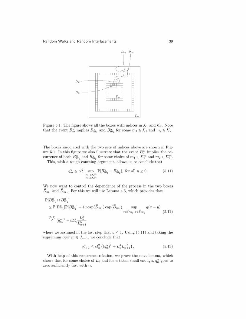
Dm2Dm2

Figure 5.1: The figure shows all the boxes with indices in K1 and K2. Notethat the event Bum implies Bum1

and Bum2for some m1 ∈ K1 and m2 ∈ K2.

The boxes associated with the two sets of indices above are shown in Fig-ure 5.1. In this figure we also illustrate that the event Bum implies the oc-currence of both Bum1

and Bum2for some choice of m1 ∈ Km1 and m2 ∈ Km2 .

This, with a rough counting argument, allows us to conclude that

qum ≤ cl2n supm1∈Km1m2∈Km2

P[Bum1∩Bum2

], for all u ≥ 0. (5.11)

We now want to control the dependence of the process in the two boxesDm1

and Dm2. For this we will use Lemma 4.5, which provides that

P[Bum1∩Bum1

]

≤ P[Bum1]P[Bum1

] + 4u cap(Dm1) cap(Dm2

) supx∈Dm1

,y∈Dm2

g(x− y)

(5.1)

≤ (qun)2 + cL2n

L2n

L5n+1

(5.12)

where we assumed in the last step that u ≤ 1. Using (5.11) and taking thesupremum over m ∈ Jn+1, we conclude that

qun+1 ≤ cl2n((qun)2 + L4

nL−5n+1

). (5.13)

With help of this recurrence relation, we prove the next lemma, whichshows that for some choice of L0 and for u taken small enough, qun goes tozero sufficiently fast with n.

40 Cerny, Teixeira

Lemma 5.2. There exist L0 and u = u(L0) > 0, such that

qun ≤c0

l2nL1/2n

(5.14)

for every u < u.

Proof of Lemma 5.2. We define the sequence

bn = c0l2nqun, for n ≥ 0. (5.15)

The equation (5.13) can now be rewritten as

bn+1 ≤ c

((ln+1

ln

)2

b2n + (ln+1ln)2L4nL−5n+1

), for n ≥ 0. (5.16)

With (5.3) one concludes that (ln+1ln)2 ≤ cL2an L

2an+1 ≤ cL4a+2a2

n . Insertingthis in (5.16) and using again (5.3), we obtain

bn+1 ≤ c1(L2a2

n b2n + L2a2−a−1n ) ≤ c1L2a2

n (b2n + L−1n ). (5.17)

We use this to show that, if for some L0 > (2c1)4 and u ≤ 1 we have

bn ≤ L−1/2n , then the same inequality also holds for n+1. Indeed, supposing

bn ≤ L−1/2n , we have

bn+1 ≤ 2c1L2a2−1n

(5.3)

≤ 2c1L−1/2n+1 L

1/2(1+a)+2a2−1n

(5.3)

≤ 2c1L−1/2n+1 L

−1/40 ≤ L−1/2

n+1 .

(5.18)

Which is the statement of the lemma. So all we still have to prove is that

b0 ≤ L−1/20 for L0 > (2c1)4 and small enough u. Indeed,

b0(5.15)

= c0l20qu0 ≤ c0l20 sup

m∈J0P[Iu ∩ Dm 6= ∅]

≤ c1L2a+20 sup

x∈VP[x ∈ Iu]

(4.3)

≤ c1L2a+20 (1− e− cap(x)u).

(5.19)

For some L0 > (2c1)4, we take u(L0) small enough such that b0 ≤ L−1/20

for any u ≤ u(L0). This concludes the proof of Lemma 5.2

We now use this lemma to show that with positive probability, one canfind an infinite connection from (0, 0) to infinite in the set Vu ∩ Zd. For


this we choose L0 and u < u(L0) as in the lemma. Writing BM for the set[−M,M ]× [−M,M ] ⊂ Z2, we have

1− η(u, (0, 0)) ≤ P[(0, 0) is not in an infinite component of Vu ∩ Z2]

≤ P[Iu ∩BM 6= ∅] + P[

there is a ?-path in Z2 \BMsurrounding the point (0, 0) in Z2

]≤(1− exp(−u · cap(BM ))

)+∑n≥n0

P[ Iu ∩ Z2 \BM contains a ?-path surrounding (0, 0) and

passing through some point in [Ln, Ln+1 − 1]× 0 ∈ Z2

](5.20)

The last sum can be bounded by∑n≥n0

∑m P[Bum] where the index m runs

over all labels of boxesDm at level n that intersect [Ln, Ln+1−1]×0 ⊂ Z2.Since the number of such m’s is at most ln ≤ cLan,

1−η(u, (0, 0)) ≤ cL2n0u+

∑n≥n0

cLanL−1/2n

(5.3)

≤ c(L2n0u+

∑n≥n0

L−1/4n ). (5.21)

Choosing n0 large and u ≤ u(L0, n0), we obtain that the percolation prob-ability is positive. So that u? > 0 finishing the proof of Theorem 5.1.

5.1 Notes

As we mentioned below Theorem 5.1, its proof is largely inspired by Propo-sition 4.1 of [43]. It illustrates well how the renormalization scheme canhelp us to deal with the dependence present in the measure Qu. We wouldlike to mention two important improvements that were developed over theabove techniques.

Sprinkling is a technique that first appeared in Section 3 of [43]. It allowsus to obtain estimates similar to that of Lemma 4.5, but by “sprinkling”some extra trajectories into the picture, one can wash away the dependenceeven further and obtain better error estimates. This technique has beenuseful later in [40] and [49] for instance.

Another modification of the renormalization we presented here, that hasbeen very efficient in boosting the decay of dependence (such as in (5.2))are the so-called decoupling inequalities. The idea behind this procedureis to create a binary tree, which encodes the occurrence of bad events invarious sub-boxes. Then, by carefully comparing the number of such treeswith the probability that they are corrupted, one obtains a bound on theprobability of bad events. This idea first appeared in [47] and [37], beinglater generalized in [44].

Renormalization tools very similar to the ones described above haveproved themselves useful in obtaining various results, both for random in-

42 Cerny, Teixeira

terlacements and for other dependent percolation processes, see for instance[50] and [22].

Remarkably, some more elaborate renormalization schemes were able toestablish the non-triviality of the phase transition that Vu undergoes at u?.More precisely, it was shown that

u? <∞ for any d ≥ 3, see Theorem 3.5 in [43], (5.22)

andu? > 0 for any d ≥ 3, see Theorem 3.4 in [36]. (5.23)

Chapter 6

Interlacement set

Up to now, we have mainly investigated the vacant set left by a randomwalk on a finite graph or by random interlacements. In this chapter we aregoing to consider the interlacement set Iu of the random interlacements,which is of course related to the trace left by random walk on a graph,X0, . . . , Xu|G|.

Contrary to the Bernoulli percolation, where by changing p to 1− p, onecan interchange the laws of open and closed sites, the interlacement set Iuis a genuine object: It cannot be obtained from Vu by a re-parametrization.Its properties should be thus studied separately.

In general, understanding of Iu is easier than of Vu. The main reasonfor this is that the independence coming from the Poisson point processstructure is easier to explore when considering the interlacement set; Iuis the trace left by the Poisson point process, not its complement. Inaddition, there is no phase transition for the connectivity of Iu, whichfurther simplifies the studies of Iu:

Theorem 6.1 ([43, 12]). For every d ≥ 3, the interlacement set Iu on Zdsatisfies

P[Iu is connected for all u > 0] = 1. (6.1)

Proof. The proof of the theorem is based on the following proposition,that is much stronger than (6.1). To state it it is useful to introduce the

following notation. We write f(n) = s.e.(n) when f(n) ≤ ce−c′nδ for some

c, c′, δ ∈ (0,∞), ’s.e.’ staying for ‘stretched-exponentially’ small. We writef(n) = 1− s.e.(n), when 1− f(n) = s.e.(n). Observe that ncs.e.(n) = s.e.(n)for any fixed c > 0. So, it is quite convenient to use this notation e.g. inthe following situation: assume that we have at most nc events, each ofprobability bounded from above by s.e.(n). Then, the probability of theirunion is s.e.(n) as well.

Recall from Chapter 3 that P denotes the law of the Poisson point processon W ? × [0,∞) defining the random interlacements and that µA,u is the

43

44 Cerny, Teixeira

map that selects from ω those trajectories which intersect A and have labelssmaller than u. Let us define Iun to be range of the trajectories intersectingB(n),

Iun(ω) =⋃

w∈suppµB(n),u(ω)

Rangew. (6.2)

Proposition 6.2. For every d ≥ 3 and 0 < u < u′,

P[Iun is connected] = 1− s.e.(n). (6.3)

P[∀w ∈ supp(µB(n),u′ − µB(n),u) is connected to Iun ] = 1− s.e.(n). (6.4)

Let us first explain how to Proposition 6.2 implies Theorem 6.1. Assumefor the moment that the claim of Theorem 6.1 is false, that is

P[there exists u > 0 such that Iu is not connected] > 0. (6.5)

Then, one can find ε > 0 and 0 < u < u′ <∞ such that

P[there exists u ∈ [u, u′] such that I u is not connected] ≥ ε (6.6)

and so,

lim infn→∞

P[there exists u ∈ [u, u′] such that I un is not connected] ≥ ε. (6.7)

This, however, contradicts Proposition 6.2 since, by the second claim ofthe proposition, the probability that I un is connected for all u ∈ [u, u′]approaches 1 as n→∞. So, (6.5) cannot be true.

We now show Proposition 6.2. The proof that we present is more com-plicated than necessary, but it has some important implications that weexplore later. It is a simplified version of some of the arguments used in[35, 34, 12].

The proof is based on the following heuristics. It is known fact thatone random walk trajectory is a two-dimensional object. Considering alltrajectories in suppµB(n),u intersecting this trajectory (including this tra-jectory), we obtain a four-dimensional connected object. Another iterationsof this procedure give us 2k-dimensional objects (if 2k ≤ d). The capac-ity of a 2k-dimensional object intersected with a ball of size n is roughlycomparable with n2k, as long as 2k ≤ d− 2. Hence, when 2k ≥ d− 2, this2k-dimensional object saturates the B(n) in terms of capacity, and anyother random walk trajectory has a non-negligible chance to hit it. Iter-ating then the construction once more, if necessary, gives an object whichis very likely hit by every other walk in suppµB(n),u, implying that Iun isconnected.

Proof of Proposition 6.2. We start the formal proof. In d = 3, 4, the propo-sition is a direct consequence of Theorem 7.6 in [25] which states that two


independent random walks in d = 3, 4 intersect (infinitely often) with prob-ability 1, and of the fact that the number of trajectories in suppµB(n),u isfinite P-a.s. Therefore we will assume that d ≥ 5 in the proof.

Will repeatedly use the following lemma.

Lemma 6.3. Let A ⊂ Zd, and x ∈ Zd be such that maxy∈A dist(x, y) ≤ r.Then, for some c > 0 depending on the dimension only

Px[HA ≤ r2 ∧HB(x,2r)c ] ≥ cr2−d cap A. (6.8)

Proof. The proof of the lemma is a variant of the proof of (4.8). The onlynon-trivial new ingredient is the observation that for x, y with dist(x, y) ≤ rthe ‘truncated Green function’ satisfies

gB(x,2r2)(x, y; r2) :=

r2∧HB(x,2r2)c∑i=0

Px[Xi = y] ≥ cg(x, y). (6.9)

We therefore omit the details and leave the proof of (6.9) and of the lemmaas exercise.

To apply Lemma 6.3 we need to estimate capacities of various collec-tions of random walk trajectories. The estimate we will use is given inLemmas 6.5, 6.6 below. We start with a technical estimate.

Lemma 6.4. Let d ≥ 5, (xk)k≥1 be a sequence in Zd, and let Xk be asequence of independent simple random walks on Zd with Xk

0 = xk. Thenfor all positive integers N and n and for all (xk)k≥1,

E[ N∑k,l=1

2n∑i,j=n+1

g(Xki , X

lj)]≤ C

(Nn+N2n3−d/2). (6.10)

Proof. Let X be a simple random walk with X0 = 0, then for all y ∈ Zdand for all positive integers k, by the Markov property,

Eg (Xk, y) =∞∑i=k

P [Xi = y] ≤ C∞∑i=k

i−d/2 ≤ Ck1−d/2. (6.11)

Here we used the inequality supy∈Zd P [Xk = y] ≤ Ck−d/2, see [38, Propo-sition 7.6] In order to prove (6.10), we consider separately the cases k = land k 6= l. In the first case, the Markov property and the fact thatg(x, y) = g(x− y) imply

E[ N∑k=1

2n∑i,j=n+1

g(Xki , X

kj )]

= NE[ 2n∑i,j=n+1

g(X|i−j|)]

(6.11)

≤ CNn(

1 +

n∑i=1

i1−d/2) (d≥5)

≤ CNn.

(6.12)

46 Cerny, Teixeira

In the case k 6= l, an application of (6.11) gives

E[ 2n∑i,j=n+1

g(Xki , X

lj)]≤ n2Cn1−d/2. (6.13)

This completes the proof.

Let (Xk)k≥1 be the collection of independent random walks, as in theprevious lemma. For A ⊂ Zd, let T kA = infi ≥ 0 : Xk

i /∈ A be the exit timeof Xk from A. For positive integers N and n, define the subset Φ(N,n) ofZd,

Φ(N,n) =

N⋃k=1

Xki : 1 ≤ i ≤ n ∧ T kB(xk,2n1/2)

. (6.14)

Lemma 6.5. For any sequence (xi)i≥1 ⊂ Zd and for all positive integersN and n,

cap Φ(N,n) ≤ CNn, (6.15)

andE cap Φ(N,n) ≥ cmin(Nn, n(d−2)/2). (6.16)

Proof. The upper bound follows from the sub-additivity of the capacity(4.13) and the fact that cap(x) = g(0, 0)−1 <∞.

We proceed with the lower bound on E cap Φ(N,n). By Kolmogorov’smaximal inequality applied coordinatewise, for each λ > 0 and n ≥ 1,

P[

max1≤i≤n

|Xi| ≥ λ]≤ n

λ2. (6.17)

Let J be the random set J = 1 ≤ k ≤ N : sup1≤i≤n |Xki − xk| ≤ 2n1/2,

and D the event D = |J | ≥ N/4. From (6.17), it follows that E|J | ≥N(1− n

4n

)≥ N

2 . Since |J | ≤ N , we get P [D] ≥ 13 .

To obtain a lower bound on the capacity, the following variational for-mula (see Proposition 2.3 [52]) is useful:

cap A = (inf E(ν))−1, (6.18)

where the energy E(ν) of a measure ν is given by

E(ν) =∑

x,y∈Zdν(x)ν(y)g(x, y), (6.19)

and the infimum in (6.18) is taken over all probability measures supportedon A.

Taking ν to be ν(x) = 2|J|n

∑k∈J

∑ni=n/2 1Xk

i = x, which is obviously

supported on Φ(N,n), we obtain

E cap Φ(N,n) ≥ E[E(ν)−1

]≥ E

[E(ν)−1;A

]. (6.20)


Therefore, in order to prove (6.16), it suffices to show that

E[( 4

|J |2n2

∑k,l∈J

n∑i,j=n/2

g(Xki , X

lj))−1

;A]≥ cmin

(Nn, n(d−2)/2

). (6.21)

Using the Cauchy-Schwarz inequality and the definition of the event D, theleft-hand side of the last display can be bounded from below by

cN2n2P (D)2(E[ ∑k,l∈J

n∑i,j=n/2

g(Xki , X

lj);D

])−1

(6.22)

Since J is a subset of 1, . . . , N, this is larger than

(N/4)2n2P (D)2(E[ N∑k,l=1

n∑i,j=n/2

g(Xki , X

lj)])−1

(6.10)

≥ cN2n2

Nn+N2n3−d/2 ≥ cmin(Nn, n(d−2)/2

).

(6.23)

This completes the proof.

Lemma 6.6. In the setting of the previous lemma, assume that for some

δ > 0, nδ ≤ N ≤ n d−42 −δ, then for every ε > 0 sufficiently small

P[

cap Φ(N,n) ≥ (Nn)1−ε] = 1− s.e.(n). (6.24)

Proof. To see that this lemma holds it is sufficient to split the trajectoriesinto nε pieces of length n1−ε and consider them separately. More precisely,observe that Φ(N,n) ⊃

⋃0≤`≤nε−1 Φ`, where

Φ` =⋃k≤N

Xk`n1−ε∈B(Xk0 ,n

1/2)

Xk`n1−ε , . . . , Xk

(`+1)n1−ε ∩B(Xk0 , 2n

(1−ε)/2).

(6.25)Using the standard random walk scaling, P [Xk

`n1−ε ∈ B(Xk0 , n

1/2)] > c forall ` ∈ 0, . . . , nε, and thus the union contains more than N1−ε termswith probability at least 1 − s.e.(n). Therefore, using the both estimatesof Lemma 6.5, the Markov property, and the assumption of the presentlemma, P [cap Φ` ≥ (Nn)1−ε|F`n1−ε ] ≥ c. P -a.s., where Fi is the σ-algebragenerated by Xk

j , k ≤ N , j ≤ i. As cap Φ(N,n) ≥ max`≤nε cap Φ`, thelemma follows easily from these facts.

Remark 6.7. Lemma 6.6 holds also for N = 1. An easy adaptation of theprevious proof is left as exercise.

48 Cerny, Teixeira

We may now prove (6.3) of Proposition 6.2. Let w1, . . . , wN be anarbitrary enumeration of suppµB(n),u, that is wk’s are random walk tra-jectories hitting B(n) with labels smaller than u. We will show that forevery k, l

P[Rangewk and Rangewl are connected within Iu] ≥ 1− s.e.(n). (6.26)

By the definition of random interlacements, N has Poisson distribution withparameter u capB(n) ∼ nd−2. Therefore, P[N ≥ nd] = s.e.(n), and thus,by the remark after the definition of s.e.(·), (6.26) implies (6.3). Withoutloss of generality, we take k = 1, l = 2 in (6.26).

Let s = s(d) = bd2c − 1. We split w3, . . . , wN into s independentPoisson processes,

µ` = µB(n),`u/r − µ`−1, ` = 1, . . . , r, (6.27)

where µ0 = δw1+ δw2

. As before, P [| suppµ`| ≥ nd−2−ε] = 1 − s.e.(n).For w ∈ W , let Tn(w) = infk ≥ 0 : w(k) /∈ B(3n) and R(w) =w(0), . . . , w(n2 ∧ Tn(w)). Set V0 = w1, A0 = R(w1), and for ` =1, . . . , r,

V` = w ∈ suppµ` : R(w) ∩A`−1 6= ∅, (6.28)

A` =⋃w∈V`

R(w). (6.29)

We claim that for all ` = 1, . . . , r and some ε > 0 small.

P[|V`| ≥ n2`−ε] = 1− s.e.(n). (6.30)

Indeed, this is trivially true for |V0|. If (6.30) holds for ` − 1, then byLemma 6.6,

P[capA`−1 ≥ n(1−ε)(2(`−1)−ε)n2(1−ε)] = 1− s.e.(n), (6.31)

When capA`−1 ≥ n2`−ε′ , then by Lemma 6.3, the probability than onerandom walk started in B(n) hits Al−1 before time n2 is bounded frombelow by cn2`−ε′n2−d = cn2`+2−d−ε′ . As µ` contains with probability 1−s.e.(n), at least nd−2−ε independent walks, at least nd−2−εn2`+2−d−ε′n−ε =n2`−ε of them hit A`−1 before the time n2, and exit B(3n), again with1− s.e.(n) probability. This completes the proof of (6.30).

From (6.30) it follows that |Vs| ≥ n2s−ε ≥ nd−3−ε, and, by Lemma 6.6and Remark 6.7, capR(w2) ≥ cn2−ε, with 1− s.e.(n) probability. Considernow random walks in Vs. After hitting As−1 the rest of their trajectoriesis independent of the past, so Lemma 6.3 once more implies that

P [XkHAs−1

, . . . , XkHAs−1

+n2 ∩R(w2)] ≥ n4−d−ε]. (6.32)


Hence, the event ’at least one walk in Vs hits R(w2)’ has probability atleast 1− s.e.(n). This implies (6.26) and completes the proof of (6.3).

The proof of (6.4) is analogous, it is sufficient to take w2 ∈ suppµB(n),u′ \suppµB(n),u.

The proof of Proposition 6.2, that we just finished, has some interestingconsequences. We actually proved that the set

Iun :=⋃

w∈suppµB(n),u

R(w) (6.33)

is with high probability connected. Since R(w) ⊂ B(3n), we see Iun ⊂ Iunis connected ‘locally’, that is one does not to go far from B(n) to makea connection. Of course, in general, Rangew ∩ B(n) 6= R(w) ∩ B(n), sowe did not show that Iun ∩ B(n) is ‘locally connected’. However, it is notdifficult to extend the previous techniques to show

P[every x, y ∈ B(n)∩Iu are connected in Iu∩B(3n)] = 1−s.e.(n). (6.34)

Another consequence of the previous proof is the following claim. Withprobability 1 − s.e.(n), for every pair w,w′ ∈ suppµB(n),u there are w =w0, w1, . . . , ws+1 = w′ ∈ suppµB(n),u such that wi intersects wi−1, i =1, . . . , s+ 1. Borel-Cantelli lemma then implies:

Corollary 6.8 (d ≥ 5). Consider (random) graph G whose vertices are alltrajectories in suppµZd,u, and whose two vertices are connected by an edgeiff the corresponding trajectories intersect. Then P-a.s., the diameter of Gsatisfies diamG ≤ bd/2c.

Surprisingly, this bound is optimal when d is odd. The correct upperbound (and in fact also the lower bound) is given in the following theorem.

Theorem 6.9 ([31, 34]). For every u > 0, the diameter of G equals dd/2e−1, P-a.s.

For even d’s, our upper bound exceeds the correct one by one. The mainreason for this is that we decided to prove s.e.(n) bounds on probabilities,which in turn forced us to loose nε it many steps. These nε’s are whatis missing in the last paragraph of the proof of Proposition 6.2 to get theoptimal bound.

Almost the same techniques, however, allow to show that (cf. (6.30),(6.32)), for all n large enough,

P[|V` ≥ cn2`−2] > c′ > 0 and P[w2 intersects As] > c′. (6.35)

In [34], estimates similar to (6.35) together with ideas inspired by Wienertest (see [26, Theorem 2.2.5]) are applied to obtain the optimal upperbound.

50 Cerny, Teixeira

Our proof of Proposition 6.2 has yet another consequence on what iscalled chemical distance on the interlacement set, defined for x, y ∈ Iu by

ρu(x, y) = minn : ∃x = z0, z1, . . . , zn = y such that

zi ∈ Iu and |zi − zi−1| = 1, i = 1, . . . , n.

(6.36)

Claim (6.34) easily yields,

P[ρu(x, y) ≤ 9nd ∀x, y ∈ B(n) ∩ Iu] = 1− s.e.(n). (6.37)

The bound 9nd is of course far from being optimal. (6.37) is however oneof the ingredients of the optimal upper bound Cn which is proved in [12]:

Theorem 6.10 ([12]). For every u > 0 and d ≥ 3 there exist constantsC,C ′ <∞ and δ ∈ (0, 1) such that

P[there exists x ∈ Iu∩[−n, n]d such that ρu(0, x) > Cn

∣∣0 ∈ Iu] ≤ C ′e−nδ .6.1 Notes

The properties of interlacement set Iu on Zd were investigated already inthe paper [43]. A weaker version of Theorem 6.1 is proved there (see (2.21)in [43]), namely, for every u > 0,

P[Iu is connected] = 1, (6.38)

which is sufficient to deduce the absence of the phase transition. The proofof [43] is based on the Burton-Keane argument [11].

Theorem 6.1 states that for every u > 0, Iu is supercritical. It is thusnatural to ask, as in the Bernoulli-percolation theory, to which extend thegeometry of Iu (at large scales) resembles the geometry of the completelattice Zd.

Recently, many results going in this direction appeared. In [35] it wasproved that Iu percolates in two-dimensional slabs, namely that for everyu > 0 and d ≥ 3 exists R > 0 such that Iu ∩ (Z2 × [0, R]d−2) containsan infinite component P-a.s. In [33] it was further shown that the randomwalk on Iu is P-a.s. transient. Theorem 6.10 is another result of this type.

Theorem 6.9, giving the diameter of the graph G, was independentlyshown by Procaccia and Tykesson [31] using ideas of stochastic dimensiontheory developed in [5], and by Rath and Sapozhnikov [34] whose methodsare commented above.

The techniques used in our proof of Proposition 6.2 are mixture of meth-ods from [34] (where we borrowed Lemmas 6.4 and 6.5) and [12] (whichcontains contains many s.e.(n) estimates).

The results of this chapter can be used to deduce some properties of thetrace X0, . . . , XuNd of the simple random walk on the torus. E.g., Theo-rem 6.10 was combined in [12] with the coupling of random interlacements


and random walk from [49] to control the chemical distance on the randomwalk trace.

Chapter 7

Locally tree-like graphs

In the previous chapters we have studied the random walk on the torusand the corresponding interlacement set on Zd. We have seen that inthat case many interesting questions are still open, including the existenceof a sharp phase transition in the connectivity of the vacant set of therandom walk, and its correspondence to the phase transition of randominterlacements. Answering these questions requires a better control of therandom interlacements in both sub-critical and supercritical phase whichis not available at present.

In this chapter we are going to explore random interlacements on graphswhere such control is available, namely on trees. We will then explain howsuch control can be used to show the phase transition for the vacant set ofrandom walk on finite ‘locally tree-like’ graphs, and to give the equivalenceof critical points in both models. In other worlds, we prove Conjecture 2.6on the locally tree-like graphs.

7.1 Random interlacements on trees

We start by considering random interlacements on trees. We will show thatvacant clusters of this model behave like Galton-Watson trees, which allowsus to perform many exact computations. As in this lecture notes we onlydeal with random walks and random interlacements on regular graphs, werestrict our attention to regular trees only.

Let Td be infinite d-regular tree, d ≥ 3, for which the simple randomwalk is transient. We may therefore define random interlacements on Tdsimilarly as we did for Zd.

We write Px for the law of the canonical simple random walk (Xn) on Tdstarted at x ∈ Td, and denote by eK , K ⊂⊂ Td the equilibrium measure,

eK(x) = Px[HK =∞]1x ∈ K. (7.1)

52


Observe that if K is connected, eK can be easily computed. Indeed, denot-ing by d(·, ·) the graph distance on the tree, we observe that under Px, theprocess d(Xn, x) has the same law as a drifted random walk on N startedat 0. If not at 0, this walk jumps to the right with probability (d − 1)/dand to the left with probability 1/d; at 0 it goes always to the right. Us-ing standard computation for the random walk with drift, see e.g. [54],Lemma 1.24, it is then easy to show that

Px[Hx =∞] = Py[Hx =∞] =d− 2

d− 1, (7.2)

for every neighbor y of x. For K connected, we then get

eK(x) =1

d#y : y ∼ x, y /∈ Kd− 2

d− 1, (7.3)

where the first two terms give the probability that the first step of therandom walk exists K.

We consider spaces W+, W , W ?, Ω and measures QK defined similarlyas in Chapter 3, replacing Zd by Td in these definitions when appropriate.As in Theorem 3.1, it can be proved that there exists a unique σ-finitemeasure ν on (W ?,W?) satisfying the restriction property (3.14). Usingthis measure, we can then construct a Poisson point process ω on W ?×R+

with intensity measure ν(dw?)⊗ du and define the interlacements at levelu and its vacant set as in (3.27), (3.28).

The main result of this section is the following theorem.

Theorem 7.1 ([46], Theorem 5.1). Let x ∈ Td and define fx : Td → [0, 1]by

fx(z) = Pz[d(Xn, x) > d(x, z) for all n > 0]

× Pz[d(Xn, x) ≥ d(x, z) for all n ≥ 0].(7.4)

Then the vacant cluster of Vu containing x in the random interlacementshas the same law as the open cluster containing x in the inhomogeneousindependent Bernoulli site percolation on Td characterized by

Prob[z is open] = exp−ufx(z). (7.5)

Remark 7.2. 1. Observe that on Td, fz(x) is the same for all z 6= x. Hence,the cluster of Vu containing x can be viewed as a Galton-Watson tree witha particular branching law in the first generation.

2. Beware that the joint law of, e.g., vacant clusters containing twopoints x 6= y ∈ Td is not the same as in the Bernoulli percolation.

Proof. We partition the space W ? into disjoint subsets W ?,z according tothe position where w? ∈W ? get closest to the given point x,

W ? =⊔z∈Td

W ?,z, (7.6)

54 Cerny, Teixeira

where

W ?,z =w? ∈W ? : z ∈ Ran(w?), d

(x,Ran(w?)

)= d(x, z)

. (7.7)

(The fact that W ?,z are disjoint follows easily from the fact that Td is atree.)

As a consequence of disjointness we obtain that the random variablesω(W ?,z × [0, u]) are independent. We may thus define independent siteBernoulli percolation on Td by setting

Y uz (ω) = 1ω(W ?,z × [0, u]) ≥ 1 for z ∈ Td. (7.8)

By (3.9), (3.14) and (7.7), we see that

P[Y uz = 0] = exp−ufx(z). (7.9)

To finish the proof of the theorem, it remains to observe that the nullcluster of (Y u· ) containing x coincides with the component of Vu containingx. The easy proof of this claim is left as exercise.

As a corollary of Theorem 7.1 and (7.3) we obtain the value of criticalthreshold of random interlacements on Td which, similarly as on Zd, isdefined by

u?(Td) = infu ≥ 0 : P[the cluster of x in Vu is infinite] = 0

. (7.10)

Corollary 7.3. The critical point of the random interlacements on Td isgiven by

u?(Td) =d(d− 1) log(d− 1)

(d− 2)2. (7.11)

Proof. For z 6= x, by considering drifted random walk as above (7.1), it iseasy to see that

fx(z) =d− 2

d− 1× d− 1

d

d− 2

d− 1=

(d− 2)2

d(d− 1). (7.12)

Hence, the offspring distribution of the Galton-Watson process mentionedin Remark 7.2 is (except in the first generation) binomial with parameters

(d−1, exp−u (d−2)2

d(d−1)). This Galton-Watson process is critical if the mean

of its offspring distribution is equal one, implying that u?(Td) is the solutionof

(d− 1) exp− u (d− 2)2

d(d− 1)

= 1, (7.13)

yielding (7.11).


Remark 7.4. For the previous result, the offspring distribution in the firstgeneration is irrelevant. Using (7.1) and Theorem 7.1, it is however easyto see that (for k = 0, . . . , d)

P[x ∈ Vu] = e−u cap(x) = e−ufx(x) = e−u(d−2)/(d−1), (7.14)

P[|Vu ∩ y : y ∼ x| = k

∣∣x ∈ Vu] =

(d

k

)e−uk

(d−2)2

d(d−1)(1− e−u

(d−2)2

d(d−1))d−k

.

(7.15)

We will need these formulas later.

7.2 Random walk on tree-like graphs

We now return to the problem of the vacant set of the random walk onfinite graphs. However, instead of considering the torus as in Chapter 2,we are going to study graphs that locally look like a tree, in hope to usethe results of the previous section.

Actually, most of this section will deal with so-called random regulargraphs. Random d-regular graph with n vertices is a graph that is chosenuniformly from the set Gn,d of all simple (i.e. without loops and multipleedges) graphs with the vertex set Vn = [n] := 1, . . . , n and all verticesof degree d, assuming tacitly that nd is even. We let Pn,d to denote thedistribution of such graph, that is the uniform distribution on Gn,d.

It is well know that with probability tending to 1 as n increases, themajority of vertices in random regular graph has a neighborhood withradius c log n which is graph-isomorph to a ball in Td.

For a fixed graph G = (V, E) let PG be the law of random walk on Gstarted from the uniform distribution and (Xt)t≥0 the canonical process.As before we will be interested in the vacant set

VuG = V \ Xt : 0 ≤ t ≤ u|V |, (7.16)

and denote by Cumax its maximal connected component.We will study the properties of the vacant set under the annealed measure

Pn,d given by

Pn,d(·) =

∫PG(·)Pn,d(dG)

(=∑G

PG(·)Pn,d[G]). (7.17)

The following theorem states that a phase transition occurs in the be-havior of the vacant set on random regular graph.

Theorem 7.5 (d ≥ 3, u? := u?(Td)).

(a) For every u < u? there exist constant c(u) ∈ (0, 1) such that

n−1|Cmax|n→∞−−−−→ c(u) in Pn,d-probability. (7.18)

56 Cerny, Teixeira

(b) When u > u?, then for every ε there is K(u, ε) <∞ such that for alln large

Pn,d[|Cmax| ≥ K(u, ε) log n] ≤ ε. (7.19)

Observe that Theorem 7.5 not only proves the phase transition, but alsoconfirms that the critical point coincides with the critical point of randominterlacements on Td. The theorem was proved (in a weaker form butfor a larger class of graphs) in [14]. In these notes, we are going to use asimple proof given by Cooper and Frieze [15] which uses in a clever way therandomness of the graph. Besides being simple, this proof has an additionaladvantage that it can be used also in the vicinity of the critical point: Bya technique very similar to the ones presented here, it was proved in [13]that the vacant set of the random walk exhibits a double-jump behavioranalogous to the maximal connected cluster in Bernoulli percolation:

Theorem 7.6.

(a) Critical window. Let (un)n≥1 be a sequence satisfying

|n1/3(un − u?)| ≤ λ <∞ for all n large enough. (7.20)

Then for every ε > 0 there exists A = A(ε, d, λ) such that for all nlarge enough

Pn,d[A−1n2/3 ≤ |Cunmax| ≤ An2/3] ≥ 1− ε. (7.21)

(b) Above the window. When (un)n≥1 satisfies

u? − unn→∞−−−−→ 0, and n1/3(u? − un)

n→∞−−−−→∞, (7.22)

then

|Cunmax|/n2/3 n→∞−−−−→∞, in Pn,d-probability. (7.23)

(c) Below the window. When (un)n≥1 satisfies

u? − unn→∞−−−−→ 0, and n1/3(u? − un)

n→∞−−−−→ −∞, (7.24)

then

|Cunmax|/n2/3 n→∞−−−−→ 0. in Pn,d-probability. (7.25)

We will now sketch the main steps of the proof of Theorem 7.5. Detailedproofs can be found in [15, 13].


7.2.1 Very short introduction to random graphs

We start by reviewing some properties of random regular graphs, for moreabout these graphs see e.g. [7, 55].

It turns out that it is easier to work with multi-graphs instead of simplegraphs. Therefore we introduce Mn,d for the set of all d-regular multi-graphs with vertex set [n].

For reasons that will be explained later, we also define random graphswith a given degree sequence d : [n] → N. We will use Gd to denotethe set of graphs for which every vertex x ∈ [n] has the degree dx =d(x). Similarly,Md stands for the set of such multi-graphs; here loops arecounted twice when considering the degree. Pn,d and Pd denote the uniformdistributions on Gn,d and Gd respectively. We say that a given event holdsasymptotically almost surely (denoted by Pn,d-a.a.s. or Pd-a.a.s dependingon the case) if it holds with probability converging to one, with respect toPn,d or Pd.

We first introduce the pairing construction, which allows to generategraphs distributed according to Pn,d, starting from a random pairing of aset with dn elements. The same construction can be used to generate arandom graph chosen uniformly at random from Gd.

We consider a sequence d : Vn → N such that∑x∈Vn dx is even. Given

such a sequence, we associate to every vertex x ∈ Vn, dx half-edges. Theset of half-edges is denoted by Hd = (x, i) : x ∈ Vn, i ∈ [dx]. We writeHn,d for the case dx = d for all x ∈ Vn. Every perfect matching M ofHd (i.e. partitioning of Hd into |Hd|/2 disjoint pairs) corresponds to amulti-graph GM = (Vn, EM ) ∈Md with

EM =x, y :

(x, i), (y, j)

∈M for some i ∈ [dx], j ∈ [dy]

. (7.26)

We say that the matching M is simple, if the corresponding multi-graphGM is simple, that is GM is a graph. With a slight abuse of notation, wewrite Pd for the uniform distribution on the set of all perfect matchings ofHd, and also for the induced distribution on the set of multi-graphs Md.It is well known (see e.g. [7] or [29]) that a Pd distributed multi-graph Gconditioned on being simple has distribution Pd, that is

Pd[G ∈ · |G ∈ Gd] = Pd[G ∈ · ], (7.27)

and that, for d constant, there is c > 0 such that for all n large enough

c < Pn,d[G ∈ Gn,d] < 1− c. (7.28)

These two claims allow to deduce Pn,d-a.a.s. statements directly from Pn,d-a.a.s. statements.

The main advantage of dealing with matchings is that they can be con-structed sequentially: To construct a uniformly distributed perfect match-ing of Hd one samples without replacements a sequence h1, . . . , h|Hd| of

58 Cerny, Teixeira

elements of Hd in the following way. For i odd, hi can be chosen by anarbitrary rule (which might also depend on the previous (hj)j<i), while ifi is even, hi must be chosen uniformly among the remaining half-edges.Then, for every 1 ≤ i ≤ |Hd|/2 one matches h2i with h2i−1.

It is clear from the above construction that, conditionally on M ′ ⊆ Mfor a (partial) matching M ′ of Hd, M \ M ′ is distributed as a uniformperfect matching of Hd \(x, i) : (x, i) is matched in M ′. Since the law ofthe graph GM does not depend on the labels ‘i’ of the half-edges, we obtainfor all partial matchings M ′ of Hd the following restriction property,

Pd[GM\M ′ ∈ · |M ⊃M ′] = Pd′ [GM ∈ ·], (7.29)

where d′x is the number of half-edges incident to x in Hd that are not yetmatched in M ′, that is

d′x = dx −∣∣(y1, i), (y2, j) ∈M ′ : y1 = x, i ∈ [dx]

∣∣, (7.30)

and GM\M ′ is the graph corresponding to a non-perfect matching M \M ′,defined in the obvious way.

7.2.2 Distribution of the vacant set

We now study the properties of the vacant set of random walk. Instead ofthe vacant set, it will be more convenient to consider the following objectthat we call vacant graph Vu. It is defined by Vu = (V, Eu) with

Eu = x, y ∈ E : x, y ∈ VuG. (7.31)

It is important to notice that the vertex set of Vu is a deterministic setV and not the random set VuG, in particular Vu is not the graph inducedby VuG in G. Observe however that the maximal connected component ofthe vacant set Cmax (defined before in terms of the graph induced by Vu inG) coincides with the maximal connected component of the vacant graphVu (except when Vu is empty, but this difference can be ignored in ourinvestigations).

We use Du : V → N to denote the (random) degree sequence of Vu, andwrite Qun,d for the distribution of this sequence under the annealed measure

Pn,d, defined by Pn,d(·) :=∫PG(·)Pn,d(dG)

(=∑G P

G(·)Pn,d[G]).

The following important but simple observation from [15] allows to re-duce questions on the properties of the vacant set Vu of the random walkon random regular graphs to questions on random graphs with given degreesequences.

Proposition 7.7 (Lemma 6 of [15]). For every u ≥ 0, the distribution ofthe vacant graph Vu under Pn,d is given by Pd where d is sampled accordingto Qun,d, that is

Pn,d[Vu ∈ · ] =

∫Pd[G ∈ · ]Qun,d(dd)

(=∑d

Pd[G ∈ · ]Qun,d(d)). (7.32)


Proof. The full proof is given in [15] and [13], here we give a less rigorousbut more transparent explanation. The main observation behind this proofis the following joint construction of a Pn,d distributed multi-graph and a(discrete-time) random walk on it.

1. Pick X0 in V uniformly.

2. Pair all half-edges incident to X0 according to the pairing construc-tion given above.

3. Pick uniformly a number Z0 in [d] and set X1 to be the vertex pairedwith (X0, Z0).

4. Pair all not-yet paired half-edges incident to X1 according to thepairing construction.

5. Pick uniformly a number Z1 in [d] and set X2 to be the vertex pairedwith (X1, Z1).

6. . . .

7. Stop when X|V |u and its neighbors are known.

At this moment we have constructed the first |V |u steps of the randomwalk trajectory and determined all edges in the graph that are incident tovertices visited by this trajectory. To finish the construction of the graphwe should

(8) Pair all remaining half-edges according to the pairing construction.

It is not hard to observe that the edges created in step (8) are exactlythe edges of the vacant graph Vu and that the degree of x in Vu is knownalready at step (7). Using the restriction property of partial matchings(7.29), it is then not difficult to prove the proposition.

Due to the last proposition, in order to show Theorem 7.5 we need aninformation about two objects: the maximal connected component of aPd-distributed random graph, and about the distribution Qun,d. We dealwith them in the next two subsections.

7.2.3 Random graphs with a given degree sequence.

The random graphs with a given (deterministic) degree sequence are wellstudied. A rather surprising fact, due to Molloy and Reed [30] is that thephase transition in its behavior is characterized by a single real parametercomputed from a degree sequence. We give a very weak version of resultof [30]:

60 Cerny, Teixeira

Theorem 7.8. For a degree sequence d : [n]→ N, let

Q(d) =

∑nx=1 d

2x∑n

x=1 dx− 2. (7.33)

Consider now a sequence of degree sequences (dn)n≥1, dn : [n] → N,and assume that the degrees dnx are uniformly bounded by some ∆ and that|x ∈ [n] : dnx = 1| ≥ ζn for a ζ > 0. Then

• If lim inf Q(dn) > 0, then there is c > 0 such that with Pd probabilitytending to one the maximal connected component of the graph is largerthan cn.

• When lim supQ(dn) < 0, then the size of the maximal connectedcomponent of Pd-distributed graph is with high probability o(n).

Later works, see e.g. [23, 21], give a more detailed description of randomgraphs with given degree sequences, including the description of the criticalwindow which allows to deduce Theorem 7.6.

7.2.4 The degree sequence of the vacant graph

We will show that the distribution of the degree sequence of the vacantgraph is the same as the distribution of the number of vacant neighbors ofany given vertex x in a random interlacements on Td. More precisely, itfollows from Remark 7.4 that the probability that x ∈ VuTd and its degreein VuTd is i, i = 0, . . . , d, is given by

dui := e−ud−2d−1

(d

i

)piu(1− pu)d−i, (7.34)

with pu = exp−u (d−2)2

d(d−1).Recall Du denotes the degree sequence of the vacant graph Vu. For

any degree sequence d, ni(d) denotes the number of vertices with degreei in d. The following theorem states that quenched expectation of ni(Du)concentrates around ndui .

Theorem 7.9. For every u > 0 and every i ∈ 0, . . . , d,∣∣EG[ni(Du)]− ndui∣∣ ≤ c(log5 n)n1/2, Pn,d-a.a.s. (7.35)

We decided to not to present the proof of this theorem in these notes, asit uses very similar arguments as the proofs in Chapter 2. The full proofcan be found in [49].

In order to controlQun,d we need to show that ni(Du) concentrates aroundits mean. This is the result of the following theorem that holds for deter-ministic graphs.


Theorem 7.10. Let G be a d-regular (multi)graph on n vertices whosespectral gap λG is larger than some α > 0. Then, for every ε ∈ (0, 1

4 ), andfor every i ∈ 0, . . . , d,

PG[|ni(Du)− EG[ni(Du)]| ≥ n1/2+ε

]≤ cα,εe−cα,εn

ε

. (7.36)

The proof of this theorem uses concentration inequalities for Lipschitzfunctions of sequences of not-independent random variables, and can befound in [13].

From Theorems 7.9 and 7.10, it is easy to compute the typical value ofQ(Du). It turns out that it is positive when u < u? and negative whenu > u?. This proves via Theorem 7.8 and Proposition 7.7 the existence ofa phase transition of the vacant set.

In fact, the above results allow to compute Q(Du) up to an additiveerror which is o(n−1/2+ε). This precision is more than enough to applythe stronger results on the behavior of random graphs with given degreesequences [21] and to show Theorem 7.6.

7.3 Notes

Theorem 7.1, that is the comparison of the cluster of the vacant set contain-ing a given point with the cluster of Bernoulli percolation, can be general-ized to arbitrary locally finite (weighted) trees. However, as the invariantmeasure of the random walk is then in general not uniform, a slight careshould be taken in defining the random interlacements, see [46].

Apart Td, there is to our knowledge only one other case where the criticalvalue of random interlacements can be computed explicitly (and is non-trivial), namely for the base graph being a Galton-Watson tree. In thiscase, it was shown in [45] that u? is a.s. constant (i.e. ‘does not depend’ onthe realization of the Galton-Watson tree) and can be computed implicitlyas a solution to a particular equation.

As we have already mentioned, a result very similar to Theorem 7.5 wasfirst proved in [14] (see Theorems 1.2 and 1.3). In [14], the proof strategyfollows a description of the local measure, with a flavor similar to that ofChapter 2, therefore it is very different from the techniques sketched in thischapter. Although we believe that the local picture approach can hardlywork to the level of precision obtained in Theorem 7.6, the class of graphsfor which this technique applies is much broader: Let us informally mentionthat Theorems 1.2 and 1.3 of [14] apply to any sequence of graphs (Gn)n≥1

such that for each n ≥ 1,

• Gn are d-regular,

• the spectral gap of Gn is bounded from below by a constant and

• there exists an ε > 0 such that every ball B(x, ε log n) in Gn has atmost one cycle.

62 Cerny, Teixeira

In [48] the interlacement set Iu was studied in various different graphs.There, special emphasis was given to the connectivity of Iu on differentclasses of graphs. More precisely, it was proven that

if G is a vertex-transitive, non-amenable graph,then, for u > 0 small enough,

the interlacement set Iu is almost surely disconnected.(7.37)

On the other hand,

if G is a vertex-transitive, amenable, transient graph,then, for all u ≥ 0, Iu is a.s. connected.

(7.38)

An interesting example is given by the product Td × Zd′ of a d-regulartree with a d′-dimensional lattice, with d ≥ 3 and d′ ≥ 1. In this case, weknow that there is a transition between a disconnected and a connectedphase for Iu as u crosses a critical threshold uc. It is worth mentioningthat this critical value has been proven in [48] to be unique, despite theabsence of monotonicity in connectivity properties of Iu.

Index

annealed measure, 55

Bernoulli (site) percolation, 32

canonical coordinates, 16canonical shift, 21capacity, 9critical window, 56

Dirac measure, 16disconnection of cylinder, 18disconnection time, 18domination, 34

entrance time, 8equilibrium distribution, 5equilibrium measure, 9excursion, 4excursions, 13

finite energy, 33

hitting time, 8

interlacement set, 25

Lebesgue measure, 23local picture, 4, 5, 7, 9

pairing construction, 57

random interlacements, 22, 25random regular graph, 55random walk

lazy, 7simple, 7transient, 8

regeneration time, 8

regular graph, 52regular tree, 52restriction property, 58reversible, 7

shift operator, 8spectral gap, 8

timedeparture, 13entrance, 21exit, 21return, 13

trajectoriesmodulo time-shift, 22

trajectorydoubly-infinite, 21

vacant set, 25vacant set in the torus, 3

63

64 Index

A, 22cap(A), 9⊂⊂, 21δ, 16eA, 9HA, 21ΛN , 8λj , 8µA, 26ν, 23Ω, 22Ω+, 16ω+, 16P , 7PA, 16?-path, 33φ, 9π, 7π?, 22Πu, 25Px, 7QA, 22QuA, 16Qu, 25Rp, 32sA, 26TA, 21Td, 52TdN , 7θk, 8, 21W , 21w0, 26WA, 21W, 21W+, 16W+, 16W ?, 22W ?

A , 22W?, 22Xn, 7, 16Y, 25Yx, 25Zd, 8

Bibliography

[1] David J. Aldous and Mark Brown. Inequalities for rare events in time-reversible Markov chains. I. In Stochastic inequalities (Seattle, WA,1991), volume 22 of IMS Lecture Notes Monogr. Ser., pages 1–16. Inst.Math. Statist., Hayward, CA, 1992.

[2] David J. Aldous and Mark Brown. Inequalities for rare events in time-reversible Markov chains. II. Stochastic Process. Appl., 44(1):15–25,1993.

[3] David Belius. Cover levels and random interlacements.arXiv:1103.2072, 2011.

[4] David Belius. Gumbel fluctuations for cover times in the discrete torus.arXiv:1202.0190, 2012.

[5] Itai Benjamini, Harry Kesten, Yuval Peres, and Oded Schramm. Ge-ometry of the uniform spanning forest: transitions in dimensions4, 8, 12, . . . . Ann. of Math. (2), 160(2):465–491, 2004.

[6] Itai Benjamini and Alain-Sol Sznitman. Giant component and vacantset for random walk on a discrete torus. J. Eur. Math. Soc. (JEMS),10(1):133–172, 2008.

[7] Bela Bollobas. Random graphs, volume 73 of Cambridge Studies in Ad-vanced Mathematics. Cambridge University Press, Cambridge, secondedition, 2001.

[8] Bela Bollobas and Oliver Riordan. Percolation. Cambridge UniversityPress, New York, 2006.

[9] Christian Borgs, Jennifer T. Chayes, Remco van der Hofstad, Gor-don Slade, and Joel Spencer. Random subgraphs of finite graphs. I.The scaling window under the triangle condition. Random StructuresAlgorithms, 27(2):137–184, 2005.

[10] Christian Borgs, Jennifer T. Chayes, Remco van der Hofstad, GordonSlade, and Joel Spencer. Random subgraphs of finite graphs. II. The

65

66 Bibliography

lace expansion and the triangle condition. Ann. Probab., 33(5):1886–1944, 2005.

[11] R. M. Burton and M. Keane. Density and uniqueness in percolation.Comm. Math. Phys., 121(3):501–505, 1989.

[12] Jirı Cerny and Serguei Popov. On the internal distance in the inter-lacement set. Electron. J. Probab., 17(29):1–25, 2012.

[13] Jirı Cerny and Augusto Teixeira. Critical window for the vacant setleft by random walk on random regular graphs. to appear in RandomStructures & Algorithms, arXiv:1101.1978, 2011.

[14] Jirı Cerny, Augusto Teixeira, and David Windisch. Giant vacant com-ponent left by a random walk in a random d-regular graph. Ann. Inst.H. Poincare Probab. Statist., 47(4):929–968, 2011.

[15] Colin Cooper and Alan Frieze. Component structure induced by arandom walk on a random graph. to appear in Random Structures &Algorithms, arXiv 1005.1564, 2010.

[16] Amir Dembo and Alain-Sol Sznitman. On the disconnection of adiscrete cylinder by a random walk. Probab. Theory Related Fields,136(2):321–340, 2006.

[17] Amir Dembo and Alain-Sol Sznitman. A lower bound on the discon-nection time of a discrete cylinder. In In and out of equilibrium. 2,volume 60 of Progr. Probab., pages 211–227. Birkhauser, Basel, 2008.

[18] P. Erdos and A. Renyi. On the evolution of random graphs. MagyarTud. Akad. Mat. Kutato Int. Kozl., 5:17–61, 1960.

[19] Geoffrey Grimmett. Percolation, volume 321 of Grundlehren der Ma-thematischen Wissenschaften. Springer-Verlag, Berlin, second edition,1999.

[20] Olle Haggstrom and Johan Jonasson. Uniqueness and non-uniquenessin percolation theory. Probab. Surv., 3:289–344 (electronic), 2006.

[21] Hamed Hatami and Michael Molloy. The scaling window for arandom graph with a given degree sequence. In Proceedings ofSODA 2010, 2010. more exhaustive version of the paper appears atarXiv:0907.4211.

[22] Marcelo Hilario, Vladas Sidoravicius, and Augusto Teixeira. Cylinders’percolation in three dimensions. preprint, 2012.

[23] Svante Janson and Malwina J. Luczak. A new approach to the giantcomponent problem. Random Structures Algorithms, 34(2):197–216,2009.

Bibliography 67

[24] Olav Kallenberg. Foundations of modern probability. Probability andits Applications (New York). Springer-Verlag, New York, second edi-tion, 2002.

[25] Gregory F. Lawler. A self-avoiding random walk. Duke Math. J.,47(3):655–693, 1980.

[26] Gregory F. Lawler. Intersections of random walks. Probability and itsApplications. Birkhauser Boston Inc., Boston, MA, 1991.

[27] Gregory F. Lawler and Vlada Limic. Random walk: a modern intro-duction, volume 123 of Cambridge Studies in Advanced Mathematics.Cambridge University Press, Cambridge, 2010.

[28] David A. Levin, Yuval Peres, and Elizabeth L. Wilmer. Markov chainsand mixing times. American Mathematical Society, Providence, RI,2009. With a chapter by James G. Propp and David B. Wilson.

[29] Colin McDiarmid. Concentration. In Probabilistic methods for algo-rithmic discrete mathematics, volume 16 of Algorithms Combin., pages195–248. Springer, Berlin, 1998.

[30] Michael Molloy and Bruce Reed. A critical point for random graphswith a given degree sequence. In Proceedings of the Sixth InternationalSeminar on Random Graphs and Probabilistic Methods in Combina-torics and Computer Science, “Random Graphs ’93” (Poznan, 1993),volume 6, pages 161–179, 1995.

[31] Eviatar B. Procaccia and Johan Tykesson. Geometry of the randominterlacement. Electron. Commun. Probab., 16:528–544, 2011.

[32] Sidney I. Resnick. Extreme values, regular variation and point pro-cesses. Springer Series in Operations Research and Financial Engi-neering. Springer, New York, 2008. Reprint of the 1987 original.

[33] B. Rath and A. Sapozhnikov. On the transience of random interlace-ments. Electronic Communications in Probability, 16:379–391, 2011.

[34] B. Rath and A. Sapozhnikov. Connectivity properties of random in-terlacement and intersection of random walks. ALEA Latin AmericanJournal of Probability and Mathematical Statistics, 9:67–83, 2012.

[35] Balazs Rath and Artem Sapozhnikov. The effect of smallquenched noise on connectivity properties of random interlacements.arXiv:1109.5086, 2011.

[36] Vladas Sidoravicius and Alain-Sol Sznitman. Percolation for thevacant set of random interlacements. Comm. Pure Appl. Math.,62(6):831–858, 2009.

68 Bibliography

[37] Vladas Sidoravicius and Alain-Sol Sznitman. Connectivity bounds forthe vacant set of random interlacements. Ann. Inst. Henri PoincareProbab. Stat., 46(4):976–990, 2010.

[38] Frank Spitzer. Principles of random walks. Springer-Verlag, New York,second edition, 1976. Graduate Texts in Mathematics, Vol. 34.

[39] Alain-Sol Sznitman. How universal are asymptotics of disconnectiontimes in discrete cylinders? Ann. Probab., 36(1):1–53, 2008.

[40] Alain-Sol Sznitman. On the domination of random walk on a discretecylinder by random interlacements. Electron. J. Probab., 14:no. 56,1670–1704, 2009.

[41] Alain-Sol Sznitman. Random walks on discrete cylinders and ran-dom interlacements. Probab. Theory Related Fields, 145(1-2):143–174,2009.

[42] Alain-Sol Sznitman. Upper bound on the disconnection time of dis-crete cylinders and random interlacements. Ann. Probab., 37(5):1715–1746, 2009.

[43] Alain-Sol Sznitman. Vacant set of random interlacements and perco-lation. Ann. of Math. (2), 171(3):2039–2087, 2010.

[44] Alain-Sol Sznitman. Decoupling inequalities and interlacement per-colation on G × Z. Inventiones Mathematicae, 187:645–706, 2012.10.1007/s00222-011-0340-9.

[45] Martin Tassy. Random interlacements on Galton-Watson trees. Elec-tron. Commun. Probab., 15:562–571, 2010.

[46] Augusto Teixeira. Interlacement percolation on transient weightedgraphs. Electron. J. Probab., 14:no. 54, 1604–1628, 2009.

[47] Augusto Teixeira. On the size of a finite vacant cluster of randominterlacements with small intensity. Probab. Theory Related Fields,150(3-4):529–574, 2011.

[48] Augusto Teixeira and Johan Tykesson. Random interlacements andamenability. to appear in The Annals of Applied Probability, 2011.

[49] Augusto Teixeira and David Windisch. On the fragmentation of atorus by random walk. Comm. Pure Appl. Math., 64(12):1599–1646,2011.

[50] Johan Tykesson and David Windisch. Percolation in the vacant set ofpoisson cylinders. to appear in Probability Theory and Related Fields,2010.

Bibliography 69

[51] David Windisch. Logarithmic components of the vacant set for randomwalk on a discrete torus. Electron. J. Probab., 13:no. 28, 880–897, 2008.

[52] David Windisch. Random walk on a discrete torus and random inter-lacements. Electron. Commun. Probab., 13:140–150, 2008.

[53] David Windisch. Random walks on discrete cylinders with large basesand random interlacements. Ann. Probab., 38(2):841–895, 2010.

[54] Wolfgang Woess. Random walks on infinite graphs and groups, volume138 of Cambridge Tracts in Mathematics. Cambridge University Press,Cambridge, 2000.

[55] N. C. Wormald. Models of random regular graphs. In Surveys incombinatorics, 1999 (Canterbury), volume 267 of London Math. Soc.Lecture Note Ser., pages 239–298. Cambridge Univ. Press, Cambridge,1999.

70

Jirı CernyFaculty of Mathematics, University of ViennaNordbergstrasse 151090 Vienna, [email protected]://www.mat.univie.ac.at/∼cerny/

Augusto Quadros TeixeiraInstituto Nacional de Matematica Pura e Aplicada (IMPA)Estrada Dona Castorina, 11022460-320 - Rio de Janeiro, [email protected]://w3.impa.br/∼augusto/

From random walk trajectories to random interlacementscerny/publications/ebp.pdf · random walk represents a corrosive particle wandering erratically through 1. 2 Cern y, Teixeira

Documents