Forward modelling The key to waveform tomography is the calculation of Green’s functions (the point source responses) Wide range of modelling methods available.

Forward modelling• The key to waveform tomography is the calculation of Green’s functions (the point source responses)

• Wide range of modelling methods available

• Very fast methods are limited (e.g., 1D, or no multiple scattering, or no turning waves, etc)

• Very complete methods are prohibitively expensive (e.g., full 3D methods, with anisotropy, attenuation etc)

Our choice is 2D, isotropic, acoustic, two-way wave equation by frequency domain finite differences

Frequency domain finite differences

• You don’t always need all the frequencies for the inverse problem

• There are easy savings for multiple source problems

• You don’t always need a long time window

• In-elastic attenuation is easy to model

• Any dispersion law for attenuation / velocity is possible

Frequency domain finite differences

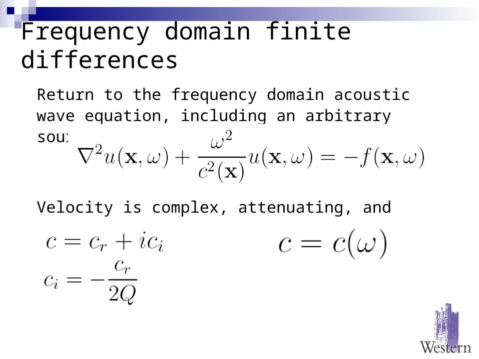
Return to the frequency domain acoustic wave equation, including an arbitrary source term:

Velocity is complex, attenuating, and dispersive:

Frequency domain finite differences

Reducing (for now) to one-dimension:

(imagine waves propagating on a string …)

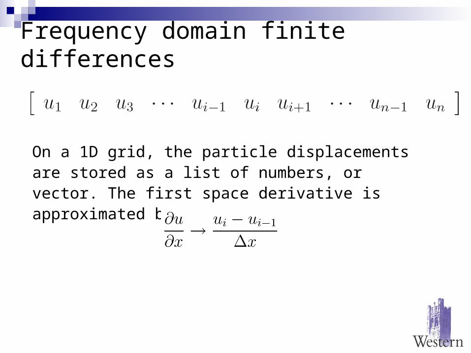
On a 1D grid, the particle displacements are stored as a list of numbers, or vector:

Frequency domain finite differences

On a 1D grid, the particle displacements are stored as a list of numbers, or vector. The first space derivative is approximated by

Frequency domain finite differences

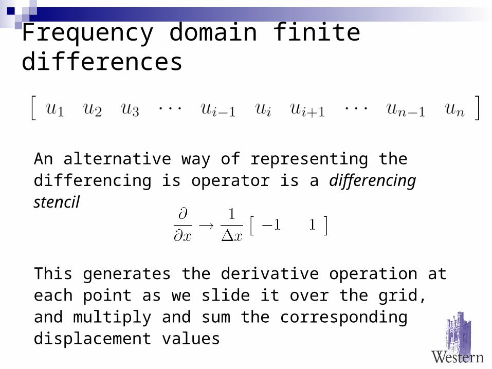
An alternative way of representing the differencing is operator is a differencing stencil

This generates the derivative operation at each point as we slide it over the grid, and multiply and sum the corresponding displacement values

Frequency domain finite differences

The second derivative differencing stencil looks like:

Frequency domain finite differences

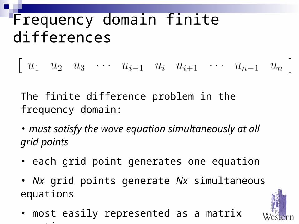
The finite difference problem in the frequency domain:

• must satisfy the wave equation simultaneously at all grid points

• each grid point generates one equation

• Nx grid points generate Nx simultaneous equations

• most easily represented as a matrix equation

Frequency domain finite differences

Frequency domain finite differences

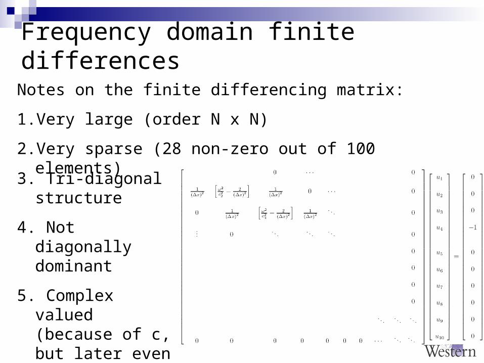
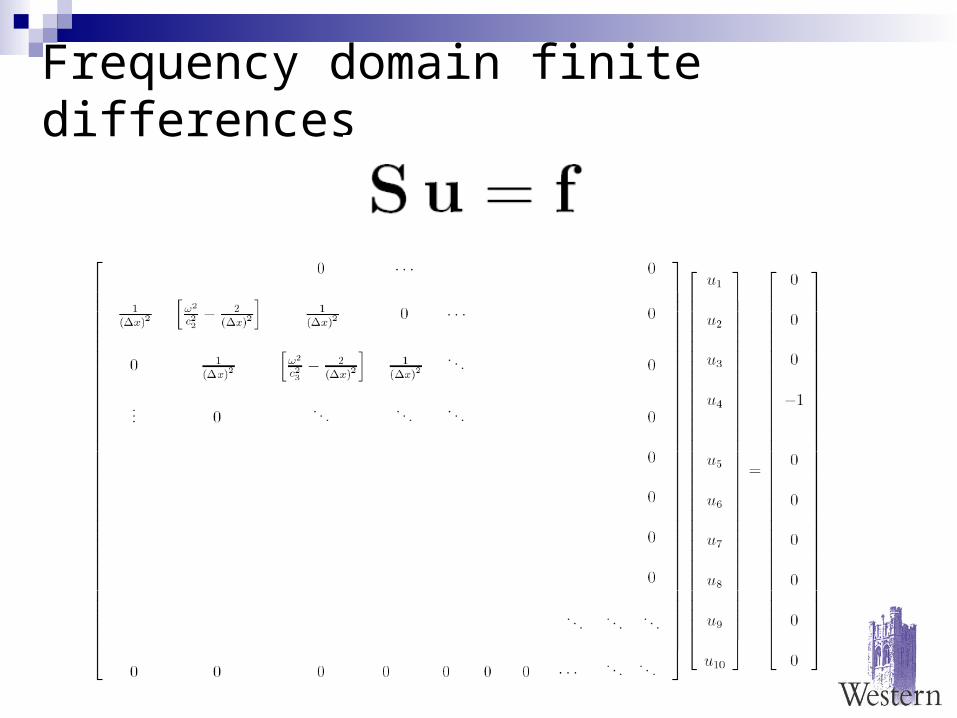
Notes on the finite differencing matrix:

1. Very large (order N x N)

2. Very sparse (28 non-zero out of 100 elements)

3. Tri-diagonal structure

4. Not diagonally dominant

5. Complex valued (because of c, but later even ω will be complex valued)

Frequency domain finite differences

Matrix differencing operators for 2D

• Wavefield is now sampled on a 2D grid

• Differencing stencils become differencing stars

Matrix differencing operators for 2D

• Wavefield is now sampled on a 2D grid

• Differencing stencils become differencing stars

For example, the second derivative in 2D could be

Matrix differencing operators for 2D

• we need to arrange the grid variables into a column vector

• assume (for now) the ordering is row-ordered:

Matrix differencing operators for 2D

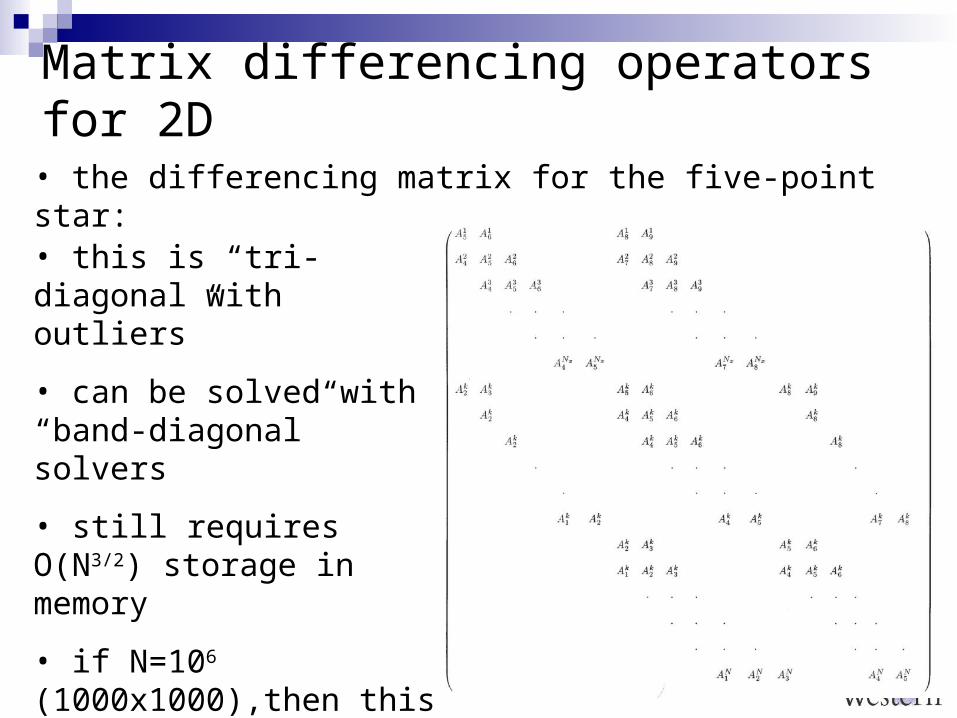
• the differencing matrix for the five-point star:

• this is “tri-diagonal with outliers”

• can be solved with “band-diagonal” solvers

• still requires O(N3/2) storage in memory

• if N=106 (1000x1000),then this is 8 Gbytes of RAM

• we need some tricks!

Tricks: Part 1 – tricks in operators

• the simple five point star differencing operator is very simple minded

• we cannot afford higher order operators, since these create additional outlier bands in the matrix

• two tricks are available: i) rotated operators, and ii) lumped and consistent mass operators

Tricks: Part 1 – tricks in operators

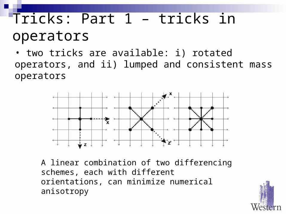
• two tricks are available: i) rotated operators, and ii) lumped and consistent mass operators

A linear combination of two differencing schemes, each with different orientations, can minimize numerical anisotropy

Tricks: Part 1 – tricks in operators

• two tricks are available: i) rotated operators, and ii) lumped and consistent mass operators

Consistent mass formulation:

Lumped mass formulation:

A linear combination of lumped and consistent mass schemes, can minimize numerical dispersion

Tricks: Part 1 – tricks in operators

• rotated operators and consistent mass matrices significantly reduce numerical dispersion (without adding outliers)

Original second order operators

Tricks: Part 1 – tricks in operators

• rotated operators and consistent mass matrices significantly reduce numerical dispersion (without adding outliers)

Rotated and consistent mass second order operators

Tricks: Part 2 – tricks in matrix solvers

• row ordering of grid leads to a band structure

• permutation of the ordering changes the matrix structure

• nested dissection recursively breaks the grid into linked sub-grids

• storage is reduced from O(N3/2) to O(N log √N)

• for N=106, storage is reduced from O(109) to O(106x3) (three orders of magnitude)

• 8 Gbyte storage requirement drops to 24 Mbyte storage (plus overhead)

Tricks: Part 2 – tricks in matrix solvers