Geophys. J. Int. (2007) 168, 723–744 doi: 10.1111/j.1365-246X.2006.03213.x GJI Seismology Formation and evolution of a population of strike-slip faults in a multiscale cellular automaton model Cl´ ement Narteau Laboratoire de Dynamique des Syst` emes G´ eologiques, Institut de Physique du Globe de Paris, 4, Place Jussieu, Paris, Cedex 05, 75252, France. E-mail: [email protected] Accepted 2006 September 4. Received 2006 September 4; in original form 2004 August 10 SUMMARY This paper describes a new model of rupture designed to reproduce structural patterns observed in the formation and evolution of a population of strike-slip faults. This model is a multiscale cellular automaton with two states. A stable state is associated with an ‘intact’ zone in which the fracturing process is confined to a smaller length scale. An active state is associated with an actively slipping fault. At the smallest length scale of a fault segment, transition rates from one state to another are determined with respect to the magnitude of the local strain rate and a time-dependent stochastic process. At increasingly larger length scales, healing and faulting are described according to geometric rules of fault interaction based on fracture mechanics. A redistribution of the strain rates in the neighbourhood of active faults at all length scales ensures that long range interactions and non-linear feedback processes are incorporated in the fault growth mechanism. Typical patterns of development of a population of faults are presented and show nucleation, growth, branching, interaction and coalescence. The geometries of the fault populations spontaneously converge to a configuration in which strain is concentrated on a dominant fault. In these numerical simulations, the material properties are uniform, so the entire process of fault development arises spontaneously from the pattern of interactions between the elements of the system over time. Furthermore, homogenization of the strain rate along faults and structural regularization of the fault trace can be quantified by analysis of the output patterns. The time dependent stochastic process allows relocation of faults by branching from bends and irregularities of the fault traces. This relocation mechanism involves partitioning of the strain and competition between faults. Possible relationships between the seismic regime and the geometry of the fault population suggest that the fault system may be attracted by a critical point. Towards this critical point, the correlation length (i.e. the length of the largest fault) increases, the proportion of large event is higher and larger faults are able to slip at lower stresses. Key words: earthquakes, fault slip, faulting, rock fracture, seismotectonics. 1 INTRODUCTION In the upper crust, an important part of the deformation occurs along fault zones via earthquakes or creep. These narrow zones of mechanical failure are surrounded by regions free of signifi- cant seismicity. Under the large scale loading system generated by plate tectonics, such a localization of the deformation in space and time implies significant stress transfer. The underlying stress ex- change mechanisms are difficult to identify because they vary on a wide range of temporal scales depending on the visco-elastic prop- erties of the upper crust, the creation of new faults and the repetition of earthquakes along them. In addition, stress is difficult to measure in situ, and geophysicists have concentrated more on the determi- nation of strain rates along faults using methods such as geodesy, paleomagnetism and carbon dating. For example, progress in dat- ing technology has enabled geologists to estimate average slip-rates along active faults during the past 10 4 to 10 5 yr (Van der Woerd et al. 2000), and paleoseismological studies indicate sequences of large earthquakes in the past 10 2 –10 4 yr (Rockwell et al. 2000). Furthermore, various analytical and empirical relationships have been proposed to link different morphological properties of active normal faults. For example, the maximum displacement on faults has been related to the length of the fault (see Cowie & Scholz 1992b; Schlische et al. 1996; Clark & Cox 1996, for a discussion of the data obtained by different workers), but also to the relative location of the fault trace with respect to the centre of the fault (Gupta & Scholz 2000) and to fault segment interactions during the formation pro- cess (Peacock & Sanderson 1991). Thus, in addition to the seismic C 2006 The Author 723 Journal compilation C 2006 RAS

Welcome message from author
This document is posted to help you gain knowledge. Please leave a comment to let me know what you think about it! Share it to your friends and learn new things together.
Transcript

Geophys. J. Int. (2007) 168, 723–744 doi: 10.1111/j.1365-246X.2006.03213.x
GJI
Sei
smol
ogy
Formation and evolution of a population of strike-slip faultsin a multiscale cellular automaton model
Clement NarteauLaboratoire de Dynamique des Systemes Geologiques, Institut de Physique du Globe de Paris, 4, Place Jussieu, Paris, Cedex 05, 75252, France.E-mail: [email protected]
Accepted 2006 September 4. Received 2006 September 4; in original form 2004 August 10
S U M M A R YThis paper describes a new model of rupture designed to reproduce structural patterns observedin the formation and evolution of a population of strike-slip faults. This model is a multiscalecellular automaton with two states. A stable state is associated with an ‘intact’ zone in whichthe fracturing process is confined to a smaller length scale. An active state is associated withan actively slipping fault. At the smallest length scale of a fault segment, transition rates fromone state to another are determined with respect to the magnitude of the local strain rate anda time-dependent stochastic process. At increasingly larger length scales, healing and faultingare described according to geometric rules of fault interaction based on fracture mechanics. Aredistribution of the strain rates in the neighbourhood of active faults at all length scales ensuresthat long range interactions and non-linear feedback processes are incorporated in the faultgrowth mechanism. Typical patterns of development of a population of faults are presentedand show nucleation, growth, branching, interaction and coalescence. The geometries of thefault populations spontaneously converge to a configuration in which strain is concentratedon a dominant fault. In these numerical simulations, the material properties are uniform, sothe entire process of fault development arises spontaneously from the pattern of interactionsbetween the elements of the system over time. Furthermore, homogenization of the strainrate along faults and structural regularization of the fault trace can be quantified by analysisof the output patterns. The time dependent stochastic process allows relocation of faults bybranching from bends and irregularities of the fault traces. This relocation mechanism involvespartitioning of the strain and competition between faults. Possible relationships between theseismic regime and the geometry of the fault population suggest that the fault system may beattracted by a critical point. Towards this critical point, the correlation length (i.e. the lengthof the largest fault) increases, the proportion of large event is higher and larger faults are ableto slip at lower stresses.
Key words: earthquakes, fault slip, faulting, rock fracture, seismotectonics.
1 I N T RO D U C T I O N
In the upper crust, an important part of the deformation occursalong fault zones via earthquakes or creep. These narrow zonesof mechanical failure are surrounded by regions free of signifi-cant seismicity. Under the large scale loading system generated byplate tectonics, such a localization of the deformation in space andtime implies significant stress transfer. The underlying stress ex-change mechanisms are difficult to identify because they vary on awide range of temporal scales depending on the visco-elastic prop-erties of the upper crust, the creation of new faults and the repetitionof earthquakes along them. In addition, stress is difficult to measurein situ, and geophysicists have concentrated more on the determi-nation of strain rates along faults using methods such as geodesy,
paleomagnetism and carbon dating. For example, progress in dat-ing technology has enabled geologists to estimate average slip-ratesalong active faults during the past 104 to 105 yr (Van der Woerdet al. 2000), and paleoseismological studies indicate sequences oflarge earthquakes in the past 102–104 yr (Rockwell et al. 2000).Furthermore, various analytical and empirical relationships havebeen proposed to link different morphological properties of activenormal faults. For example, the maximum displacement on faultshas been related to the length of the fault (see Cowie & Scholz 1992b;Schlische et al. 1996; Clark & Cox 1996, for a discussion of the dataobtained by different workers), but also to the relative location ofthe fault trace with respect to the centre of the fault (Gupta & Scholz2000) and to fault segment interactions during the formation pro-cess (Peacock & Sanderson 1991). Thus, in addition to the seismic
C© 2006 The Author 723Journal compilation C© 2006 RAS

724 C. Narteau
catalogues, paleoseismic and geological analysis of active faults aswell as geodetic measurements of coseismic and interseismic strainenable geophysicists to constrain faulting processes.
This paper presents a model of rupture whose outputs can becompared with various aspects of the structural patterns observedin the formation and evolution of a population of strike-slip faults.This work forms the second step (i.e. tectonic part) towards a gen-eral model of the spatial and temporal structures associated withthe earthquake phenomena. The first step (i.e. seismological part) isdeveloped in Narteau (2006) and consists of a detailed descriptionof the temporal properties of the seismicity observed in a model ofa single in-plane fault zone. In this model, a hierarchy is imposedand cells of different length scales represent blocks of rock of differ-ent dimensions (Narteau et al. 2000). Earthquakes are consideredas critical phenomena that occur when fractured domains organizethemselves at all length scales. Practically, a real-space renormal-ization technique is applied to the rupture problem (Kadanoff 1966;Reynolds et al. 1977; Allegre et al. 1982). From the distribution ofthe broken cells at the microscopic length scale, the state of frac-turing is obtained at increasingly larger length scales by applyinga geometric failure criterion to independent 2 × 2 lattices of cells.In a hierarchical system, the implementation of this failure crite-rion is described as an inverse cascade of fracturing and healing(i.e. transfer of the state of fracturing from smaller to larger lengthscales). When elements fail at larger length scale the redistribu-tion of the stress in their neighbourhoods applies not only at themacroscopic length scale, but also at the microscopic length scale.Because the cascade of fracturing implies failures at all interme-diate length scales, the redistribution mechanism is described as adirect cascade of stress redistribution (i.e. transfer of the stress fromlarger to smaller length scales). The multiscale cellular automatonpresented here retains similar cascade mechanisms, but differs fromthe model of seismicity in several important respects for the problemof fracture growth.
In Narteau (2006), the loading is constant and external perturba-tions are only discussed from a conceptual point of view in terms ofinstantaneous and finite stress variations. In natural data, there is agrowing body of evidence that indicates that neighbouring faults in-teract and that fracturing processes at every length scale are stronglydependent on the interrelated evolution of pre-existing faults. Thisevidence, coupled with the geomorphological observations of ac-tive tectonic regions, reveals that only a model consisting of a setof interacting faults can integrate the most important ingredientsof the fracturing process on a regional length scale (>10 km). Thepurpose of this article is not to study the seismic sequences resultingwith a model of fault interaction; rather, I apply a time-dependentstochastic model with a finite number of states at the length scale ofa fault segment in order to capture essential patterns of fault growthsuch as the geometry of the faults or the deformation accommo-dated along faults over different time intervals. Then, if the strainrates along the different faults can be quantified, they can be used inthe future as the inputs to a model of fault interaction. An importantreason for focusing on the development of fault populations is thatonly through comparison with both tectonic and seismic databasescan the prediction of a numerical modelling become more relevant.
Over the last ten years, the modelling of fracture populations hasbecome a well-established approach with a large variety of applica-tions (e.g. reservoir and aquifer characterization, reaction and trans-port phenomena). It is beyond the scope of this paper to compare indetail the present model with all previous investigations. However,different studies are single out in order to illustrate some advantagesof this new model. An & Sammis (1996) have developed a cellular
automaton which reproduces some characteristics of the geometryof crustal shear zones. In this paper, in addition to the shape of afault population, the local tectonic regime along the faults is anal-ysed. The approach is similar to that of Cowie et al. (Cowie et al.1993; Miltenberger et al. 1993; Sornette et al. 1994; Cowie et al.1995; Cowie 1998) in which the question of the self-organization ofan evolving population of fault has been addressed. Nevertheless,in the model presented here, the fault is not defined by a repetitionof earthquake ruptures. Instead, the fault zone and the local tec-tonic regime are defined via a local strain rate determined from thelong-term history of the fault system. The idea is that an individualearthquake is an expression of the localization of the deformationbut not the cause of such localization. Thus, the microfracturingprocess integrated over long time periods determines the geome-try of the fault and any one earthquake is merely a particular anddiscontinuous expression of this long-term process. Moreover, thisallows the incorporation of the analysis of different modes of dissi-pation (earthquakes, creep). In fact, aseismic deformation such aspost-seismic slip (Langbein 1990), slow earthquakes (Dragert et al.2001) and creep (Simpson et al. 2001), may comprise an importantpart of the deformation that is not included in models that consideronly repeated individual earthquakes. Another difference with theapproach of Cowie et al. (1993) is that all material properties areuniform.
2 A M O D E L O F D E V E L O P M E N T O F AP O P U L AT I O N O F S T R I K E - S L I P FAU LT S
The development of the whole system is determined by the orienta-tion of the tectonic loading and the pattern of pre-existing damage.The compressive principal stress orientations are taken to be North-South ((σ 1), vertical (σ 2,) and East–West (σ 3), in such way thatonly vertical strike-slip fault segments can form. In addition, pre-existing damage favours right-lateral faults and new segments growfollowing a main direction, at an angle � from the North (Fig. 1).
2.1 The length scale of a fault segment
A 2-D regular lattice of cells of the length scale K (hereafter calledK-cells) represents a portion of a crustal shear zone. FollowingNarteau et al. (2000), each K-cell is associated with a concep-tual picture of a fault zone: a volume within which a myriad ofmicrofractures may develop and organize themselves at all lengthscales k, 0 ≤ k ≤ K (Aviles et al. 1987). L is the size of theregular lattice. The indices (x, y), x ∈ [1,L], y ∈ [1,L] label theNorth–South and West–East coordinates, respectively. EveryK-cellis noted CK
(x,y). At any time t, CK(x,y) is defined by its state of fracturing
(a boolean variable) and a local strain rate (a scalar ε(x, y, t)).The two possible states of fracturing are (Fig. 1a)
(i) active: the fault segment interacts with adjacent active seg-ments. The fracturing process reaches the length scale K. The localbalance between the dissipation and the external forcing sustains ahigh density of microfractures which are coherently organized at alllength scales.
(ii) stable: the fault segment does not interact with adjacent ac-tive segments. Two physical representations are invoked. (1) thefracturing process does not reach the length scale K. The local bal-ance between the dissipation and the external forcing sustains a lowdensity of microfractures. They are uniformly distributed through-out the volume and they do not interact coherently. (2) Non-optimal
C© 2006 The Author, GJI, 168, 723–744
Journal compilation C© 2006 RAS
Development of a population of strike-slip faults 725
σ
σ
σ
σ1
1
3
3
Θ
stable stateactive state
K Scale
+K
KKK
KK
North
σσ
σ σ
1
13
3
(b)
(c)
(a)
Figure 1. (a) The two states of fracturing used in the model: an active state represents an actively slipping fault segment; a stable state represents an ‘intact’zone in which the fracturing process is confined to smaller length scales. σ 1 is north–south, σ 3 is east–west and only vertical dextral strike-slip faulting withan inclination � from σ 1 can develop (� ≈ 300). (b) A model of a fault population: within a 2-D regular lattice of stable cells (white cells), the fault networkis made of active segments (black cells). σ 1 and σ 3 define the principal axes of the 2-D regular lattice of cells. (c) Schematic representation of the multiscalesystem: every 2 × 2 lattice of K-cells, or grid knot, is associated with a (K + 1)-cell. This operation is repeated until a unique cell remains.
geometrical organization at the boundary of the segment temporarilyimpedes its interaction with adjacent active segments.
The scalar ε(x, y, t) attached to CK(x,y) is the local strain rate.
Ideally, it combines the effect of the external tectonic forcing andfault interactions. εa represents the external tectonic forcing and theboundary condition
εa = 1
L2
L∑i=1
L∑j=1
ε(i, j, t) = const. (1)
is maintained throughout the model run to represent the constantexternal forcing that is observed in geodetic observations of tectonicstrain (DeMets et al. 1994).
2.2 Evolution of an individual fault segment
At the length scale of a fault segment, the dynamic system is de-scribed by a time-dependent stochastic process. This process is de-
fined with respect to non-stationary transition rates between the twostates of fracturing.
The transition rate from active to stable is associated with a heal-ing process. In the most general case, the healing rule (change instate from active to stable) would occur at a rate that depends on thelocal strain rate (positive for strengthening, and negative for weak-ening). In the present work, for the sake of simplicity, the healingrate is taken as a constant, independent of position and time
αs(x, y) = γ. (2)
In later work, this simplifying assumption will be relaxed.K-cells may become active when the local strain rate exceeds a
critical value εc. At the critical strain rate εc, the density of microfrac-tures within the fault zone is high enough to allow their organizationthrough increasingly larger length scales up to the length scale Kof the fault segment. εc at each point in the grid is uniform, and itsvalue does not change with time. The transition rate from stable to
C© 2006 The Author, GJI, 168, 723–744
Journal compilation C© 2006 RAS

726 C. Narteau
active is:
αc(x, y) =
0 for ε(x, y) ≤ εc
ka
(ε(x, y) − εc
εc
)for ε(x, y) > εc
(3)
where ka is a constant with units of the inverse of a time. αc dependson the difference between the local strain rate and the threshold ofactivity. Thus, elements are capable of being active when ε > εc
and larger strain rates are associated with larger transition rates.Therefore a growing fracture accelerates according to an increasingvalue of the strain rates at the fracture tip.
2.3 The fault
If a fault segment becomes active, it can be a sub-segment of afault or a fault nucleus. In either case it interacts with the wholesystem. The distribution of active cells within the array of stablecells corresponds to a map view of the fault population assumingthat every fault zone has a constant width and a depth determinedby the thickness of the brittle crust (Fig. 1b). A fault is an isolatedset of adjacent segments which can rupture during a single event(Harris & Day 1993). More precisely, faults are defined by the so-called fault-orientation neighbourhood rule (Fig. 2). At the lengthscale K, two active segments are part of the same fault if they arenearest neighbours or second nearest neighbours in the fault-strikedirection.
Fig. 3 shows the most frequent geometric patterns of neighbouringactive fault segments in the model and how they are associated withreal tectonic structures. Most of the time, parallel fault segments(parallel faulting in Fig. 3) can be produced by the overlapping offaults growing towards each other. On the other hand, fault branchingresults from a coalescence process occurring at smaller length scales(k < K).
A new fault segment is included in a fault composed of nF (K)cells (say CK
F ). This new fault perturbs the strain rates in its neigh-bourhood according to its interaction with the other faults.
NW
S
N
SE
Figure 2. A fault orientation neighbourhood rule in a regular rectangulargrid: at the length of a fault segment, active cells aligned in the N–S, E–Wand NW–SE directions belong to the same fault of a larger length scale. Sixpossible connections are noted, N, S, E, W, NW and SE according to therelative positions of the grey-fault segments with respect to the black one(see text and Fig. 3).
2.4 Multiscale system of fault interactions
Geometric rules of fault interaction determine the state of fracturing(active or stable) at larger length scales.
2.4.1 The multiscale system
The multiple scale system is obtained as follow: every 2 × 2 latticeof K-cells corresponds to a cell of the larger length scale K+1. Thesame operation is repeated at increasingly larger length scales untila unique cell of length scale K + K remains (K = L − 1). Thus, acell of length scale K + n − 1 is associated with any n × n latticeof K-cells (Fig. 1c). (L − k + K) is the size of the regular squarelattice of length scale k ∈ {K,K + 1,K + 2, . . . ,K + K }. A cellof length scale k, Ck
(x,y), x ∈ [1,L − k + K], y ∈ [1,L − k + K]is a k-cell and �i (Ck
(x,y)) are the i-cells included in Ck(x,y)(i < k) or
composed by Ck(x,y)(i > k). Thus, �k(Ck+1
(x,y)) is the 2 × 2 lattice ofk-cells included in a cell of the larger length scale.
This multiscale system differs from the hierarchical system usedin renormalization group theory essentially because the scaling isdone at all length scales up to the largest one. Real-space renormal-ization techniques consist of dividing up a lattice of spacing s intolattices of spacing Rs,R2s,R3s and so on (Turcotte 1997). Thusthe scaling can only be done at an integer power of the renormaliza-tion factorR, a positive integer. As a consequence, a cell is includedonly in one cell at a higher level of hierarchy. In the multiscale sys-tem presented in this paper, any cell at a lower scale is included inseveral neighbouring cells of a higher scale. These intersections ofthe �i (Ck
(x,y)) with i > k are key to obtaining any localized patternswithin a system with different scales. In particular, this is requiredto produce the detail of the concentration of the strain rates at allpossible growth steps.
2.4.2 The inverse cascade of fault interaction
Lattices with different dimensions represent the brittle crust at dif-ferent length scales. A k-cell with k > K can be stable or active,depending on whether or not the internal organization of its faultsegments achieves the length scale k. At every appearance or con-solidation of an active fault segment at the smallest length scale,the configuration of the K-cells instantaneously determines all thestates of fracturing with respect to a rule of interaction applied fromthe smaller length scale to larger ones (i.e. inverse cascade of faultinteraction). Thus a geometric criterion of fault interaction is im-plemented at all length scales. Based on basic mechanical consider-ations, this criterion introduces a coarse-graining that may connecttwo neighbouring faults laterally if they have an overlap to separa-tion ratio greater than one.
In rock mechanics, the full elastic stress field should depend onshort-range interactions between neighbouring growing fracturesas well as on the long-range interactions imposed by the growth ofindividual fractures (Rodgers 1980; Mann et al. 1983; Mandl 2000).If there is no overlap between two fractures, the simple superpositionof the two stress fields is sufficient to describe the interaction. If thereis a significant overlap, say l, compared to the crack separation d, theeffective length of the crack becomes equivalent to the total lengthof the two cracks. In the present model, this short range interactionis taken into account and a lateral transfer of the active state isapplied at increasingly larger length scales of the multiscale systemif l/d > 1. This introduces a binary switch that connects the twofaults at larger length scales if this condition is met, and neglects the
C© 2006 The Author, GJI, 168, 723–744
Journal compilation C© 2006 RAS

Development of a population of strike-slip faults 727
Same segment Pull appart or bend
Branching BranchingParallel faulting or push-up
Figure 3. Schematic representations of the faulting patterns associated with different configurations of neighbouring active cells. Parallel faulting is likelyto result from external perturbations. For example, it can be associated with the overlapping of parallel growing faults. The two branching examples indicatesymmetric fault segment configurations.
interaction if it does not. That is, the magnitude of the redistributionof the strain rates is now proportional to the sum of the strain rateson the two individual segments. The two faults effectively becometwo segments of a single larger fault at the largest length scale whilestill retaining their distinctive behaviours at smaller length scaleswhere the overlap to separation ratio is less than one.
In the numerical simulations, a purely geometric failure criterionis applied at increasingly larger length scales. This failure crite-rion consists of two cooperative configurations of k-cells within�k(Ck+1
(x,y)) (Fig. 4a). These configurations involve neighbouring ac-tive cells aligned along the N–S or the NW–SE directions. Becauseactive cells model vertical fault segments oriented following themain direction, these configurations correspond to the overlap ofthe shear and extensional zones associated with right-lateral strike-slip motions along each segment. Each cell of these cooperativeconfigurations is oriented ‘up’ or ‘down’ with respect to its relativeposition along the the σ 1-direction (Fig. 4b). This polarity ‘up’ or‘down’ then points in the direction of potential crack growth. Ck+1
(x,y)
is active if one of the upper cells of �k(Ck+1(x,y)) is ‘up’ or if one of the
lower cells of �k(Ck+1(x,y)) is ‘down’ (Fig. 4c). Thus, at larger length
scales, elements are considered active if the upper half of these largeelement contains at least one ‘up’ polarity, or the lower half containsat least one ‘down’ polarity.
Simple examples of the implementation of this inverse cascadeof fault interaction are shown in Figs 4(d) and (e). Practically, faultsinteract positively with one another when, together, they sustain anactive cell at a length scale larger than their dimensions. At thelength scale of a fault segment, a fault which has a dimension Lin the σ 1 direction (i.e. North-South) makes active all the domainslocated within a rectangular area. This rectangular area is definedby the upper left corner located at L K-cells at the left from thenorthern fault tip and the lower right corner located at L K-cells atthe right from the southern fault tip (dotted area on Fig. 5). Conse-quently, if a fault is completely located within the rectangular areaof another fault, they do not positively interact together but they canpositively interact with other faults. Positive interactions are onlypossible between two faults which have their tips included in theinteracting zones of the other fault. Because of the overlap to sepa-
ration ratio, small fault tips have to be located closer to each other.Thus, within the rectangular area of one fault, the dimension of theinteracting zone varies according to the length of the neighbour-ing faults (dashed area on Fig. 5). Larger zones are associated withlonger neighbouring faults and they include all the smaller zonesfor shorter neighbouring faults.
For any transition from stable to active at the length scale K ofa fault segment, all states are recalculated, and the largest lengthscale at which a cell experiences a transition from stable to active isdefined as k m .
2.5 Strain rate redistribution
The redistribution rule for the strain rate parameter is based on asimplified template that mimics the basic anisotropy of the redistri-bution of Coulomb stresses σ C for a right-lateral strike-slip shearcrack. The Coulomb stress is the sum of the mean stress and theproduct of the local shear stress and the friction coefficient, heretaken to be µc = 0.6. Theoretically the local stress tensor (fromwhich the normal and shear stresses can be extracted) is related tothe distance r from the crack tip, the angle θ from the crack axis, by
σi, j = Kk(2πr )−1/2 fi, j (θ ), (4)
where K k is a stress intensity factor that depends on the mode offracture. For an isolated crack
Kk = Yσ l1/2, (5)
where Y is a dimensionless geometric constant, σ is the remoteapplied stress, and l the length scale of the crack. To relate theCoulomb stresses with strain rates, the redistribution is chosen toapproximate a viscous rheology. Then, the strain rate variation isequal to the stress variation multiplied by the dynamic viscosity ν,
�ε = ν�σC . (6)
The tectonic rates are redistributed only after the appearance ofa new active fault segment in the neighbourhood of the fault alongwhich the stable to active transition has taken place. Along thisfault, individual fault segments may line up following the N–S, the
C© 2006 The Author, GJI, 168, 723–744
Journal compilation C© 2006 RAS
728 C. Narteau
x
x
σ1
σ1
σ3 σ3
(a)
(b)
(c)
orientation
configurationscooperative
minimalactivatingconfigurations
scale k (e)
(d)
scale k
scale k+1
scale k+1
scale k+2
Figure 4. (a) Cooperative configurations of active cells. These configurations are those for which the shear and extensional zones associated with motionsalong dextral vertical strike-slip fault overlap. (b) Orientation of active cells in cooperative configurations: according to the direction of potential fault growth,the upper cell is ‘up’ while the lower cell is ‘down’. (c) Minimal configurations of active cells that sustain an active state at the larger length scale. (d) and (e)are examples that show how the state of fracturing is determined at increasingly larger length scales. For each example, active cells are in black, stable cellsincluded in an active cell of the larger length scale are marked with a dot, stable cells included in an active cell of the second larger length scale are markedwith a cross. Cooperative doublets are oriented. The inset shows the orientations of σ 1 and σ 3.
E–W and NW–SE directions (Fig. 2). Thus three redistribution pat-terns are associated with these three different geometries of verticalstrike-slip faults. These redistribution patterns are a coarse-graineddiscrete version of the theoretical change in Coulomb stress. Sincethis fracture problem is rotationally symmetric, four parameters areused to define these redistribution patterns. In a cellular grid, this isthe minimum number required to account for an anisotropic redistri-bution, and the resulting feedback to the strain rate on the active andstable elements. Finally, 12 independent parameters determine theshape of the redistribution (the Q parameters, see Appendix A andFig. 6). These parameters are fixed so that eq. (6) is maintained andso the inferred stress redistribution is similar to that of a Coulombredistribution at a macroscopic length scale (see Fig. 6).
To determine the direction of potential fracture growth, each re-distribution pattern is divided into two parts. Then, six global masksMd are associated with each direction d ∈ {N, NW, W, S, SE, E}.These masks are applied to all the fault segments composing thefault where the stable to active transition has occured. For an iso-
lated fault segment, these masks are non-zero on the nearest and thenext-nearest neighbours. For fault segments of larger faults, thesemasks are non-zero within larger zones. These zones have a size thatvaries according to the relative positions of the fault segments alongthe fault. Their geometries are determined by the shape of the masksaccording to the local configuration of fault segments (Fig. 6 centralcolumn). Thus, the redistribution mechanism can be described as adirecte cascade because the geometry of the fault at all length scalesdetermines the local variations of the strain rates and, for example,the spatial extension of the process zone (Fig. 6).
In making calculation, the first step consist of identifying thefault that include the new active fault segment (i.e. CK
F ). After, eachfault segment is associated with a matrix which determines the localredistribution process (Fig. 7a). This matrix consists of columns forthe NW propagation directions and the SE propagation directions(Fig. 7b). The three components of each column are determined bythe geometry of the fault-orientation neighbourhood rule: diagonal(NW and SE),vertical (N and S) or horizontal (E and W). These
C© 2006 The Author, GJI, 168, 723–744
Journal compilation C© 2006 RAS

Development of a population of strike-slip faults 729
3
σ1
σ1
σ3σ
L cells
L cellsL
cel
lsK+1
K+2
K+3
K+4K+4
K+3
K+2
K+1
K+1
K+2
K+3K+3
K+2
K+1
K+4K+4
Figure 5. A fault of length L following σ 1 activate all the K-cells locatedwithin a rectangular zone. This zone is defined by (1) a top left corner locatedat L K-cells at the left from the northern fault tip and (2) a bottom right-handcorner located at L K-cells at the right from the southern fault tip (dottedcontour). In order to positively interact with this fault, a neighbouring faulthas to end within the zones limited by the internal dashed contours. Differentcontours are for different lengths of neighbouring faults. The number ofcontours is proportional to L.
element are noted edi , d ∈ {N, NW, W, S, SE, E}, i ∈ CK
F . edi is null
if the i-cell has no active neighbour in the direction associated withthe other column. If ed
i has an active neighbour in this direction,its value is equal to the size of the square-lattice of K-cells thatcapture the remainder of the fault in the direction associated withthe other column (note the connection with the multiscale systemand see examples in Fig. 7c). The NW and SE components are atleast 1 to take into account the orientation of a fault segment at thesmallest length scale. Each matrix component, d ∈ {N, NW, W, S,SE, E}, length scale, m ∈ [K,K + K ], and K-cell, a ∈ [1,L], b ∈[1,L], is associated with a mask Md
{m,a,b}. Thus, the total strain rateperturbation mask is
ϒ(x, y) = ρεa
√km
∑o∈CK
F
∑p∈{N ,...,E}
M p
{e po ,xo,yo}(x, y) (7)
where ρ is a constant, εa is the magnitude of the external forcingsystem and (x o, yo) are the coordinates of the o-cell in the 2-Dlattice. Fig. 6 shows ϒ for different fault geometries and differ-ent values for Q parameters. In Appendix A, note that the strainrate perturbation decays as r−2 with respect to the distance fromthe fault segment (the solution for a point dislocation). The over-lapping of the zones of redistribution associated with each seg-ment imposes this decay. When all the masks are applied, near thefault tips, the strain rate perturbation decay as
√r (the solution
for a crack, eq. 4). Further, the decay of the strain rate perturba-tion accelerates and far from the fault an exponential decay may bedescribed.
Similar ingredients are present in eqs (4) and (5) and in eq. (7) toaccount for fracture geometry, fracture length or loading condition.Thus, in the present model, from the transition rates (eqs 2 and 3)and the redistribution of the strain rates (eq. 7) a positive feedback
in the fault growth mechanism may be described. A particularityof the redistribution mechanism developed in this paper is that thegeometry of the fault at all length scales controls the shape and theamplitude of the strain rate perturbation. The
√km dependence in
eq. (7) makes the redistribution sensitive to short range interactionsbetween neighbouring faults. In addition, two faults with a similarsize may have different strain rates along them. Overall, the activityof a fault depends more on its geometry, its location and its shortrange interactions than on its length.
The process zone is the neighbourhood of the fault in which thestrain rate perturbation is positive. The shadow zone is the neigh-bourhood of the fault in which the strain rate perturbation is negative.In order to respect the constant external forcing (eq. 1), the redistri-bution mechanism corresponds to a reorganization of the strain ratesthat conserves the overall ‘tectonic’ strain rate εa . The formation offaults and their growths are then only possible through regions inwhich strain rates are large enough to create and maintain new ac-tive structures. The details of the redistribution of the strain rate aregiven in Appendix B.
By definition, active fault segments have a high density of mi-crofractures and can be considered weaker than the stable regionsbetween them. Consequently, the strain rates available in the shadowzone are first redistributed along active fault segments and thenwithin the stable region of the process zone. At the end of thesetransfers, the fault, which is the weakest part of the region where theredistribution takes place, concentrates the remaining strain rates.Thus the evolution of a fault affects the strain rate along neighbour-ing faults. If a fault is located within the process zone of a growingfault, its strain rates increase. If it is located within the shadow zone,its strain rates decrease. Therefore fault growth is not only possibleinto a stable region under a significant load but also into the shadowzones of other faults.
In addition to the redistribution process, variations of the strainrates may be due to a diffusion process which allows the system toreach a homogeneous state under extremely low tectonic loading.As in the friction model developed in Narteau et al. (2000), the localstrain rate heterogeneities slowly decrease in time following a rateasymptotically proportional to the square root of time:
ε(x, y, t + �t) = εa + 1√1 + ��t
(ε(x, y, t) − εa) (8)
where � is a reduced diffusion coefficient with units of the inverseof time.
3 E V O L U T I O N O F FAU LT PAT T E R N S
In the numerical simulations, if an element adjacent to the modelboundary becomes active, then the redistribution of the strain ratesoutside the model grid is neglected. As in conventional laboratorytests, such a zero boundary condition introduces an edge effect wherethe largest faults grow preferentially in the middle of the modelspace.
An important aspect of the model is that the time step �t foreach iteration is not constant, but is determined by a generalizedPoisson process (see the appendix of Narteau et al. (2001)). Thus, forthe entire system, the time interval between two events is inverselyproportional to the sum of the transition rates,
�t = − 1∑Li=1
∑Lj=1
a(i, j)log(R). (9)
C© 2006 The Author, GJI, 168, 723–744
Journal compilation C© 2006 RAS

730 C. Narteau
Figure 6. Each line corresponds to an idealized strike of the fault: from top to bottom the fault is successively northwest↔southeast, north↔south, east↔west.The centre column shows a schematic representation of the shape of the masks. The Q parameters are symmetric with respect to the centre of the fault (QNW
i =QSE
i , QNi = QS
i , QWi = QE
i ). The left and right column show two redistributions for two sets of Q parameters: the tip-type mask (QNW = [2, 1, −1, −7],QN = [1, −4, 0, −1], QW = [−2, 4, 0, 0]) generates a process zone at each extremities of the fault and a shadow zone all along the fault; the lobe-typemask (QNW = [2, −2.5, 1.5, −7], QN = [2, −4, −1, 2], QW = [−0.5, 2, −1.5, 1]) generates an alternation of process zones and shadow zones with typicallobe-shaped patterns. In this paper, only the the fault tip mask is applied because it results from the simplest coarse-graining technique of the elastic solution.
with
a(i, j) ={
λc(i, j) if the cell is stable,
λs(i, j) if the cell is active,(10)
and R a real number randomly chosen between 0 and 1.At t = 0,K-cells are all stable, strain rates are uniform and
larger than the critical value εc (i.e. εa > εc), so that at least onefailure is bound to occur to nucleate the process. Then, the re-distribution mechanism produces a heterogeneous strain rate dis-tribution. From eq. (3), the time step depends on the level ofconcentration of deformation, ensuring that larger fractures growmore quickly, and intact zones at high strain rate break morerapidly.
Once the first element becomes active the chance of a futureelement making a transition is now not uniform. Instead the nextelement to make a transition is determined by a weighted probabil-ity, where intact elements having a high strain rate are proportion-ately more likely to become active. For a given time interval this
probability is
P(x, y) = a(x, y)∑n
i=1
∑m
j=1a(i, j)
. (11)
Numerically, we define a cumulative step function ranging from 0to 1, where jumps are proportional to the P(x, y)-values. Then, wedraw at random a value between 0 and 1. This value falls within ajump of the cumulative step function which determines in turn thecell which experiences a transition.
This temporal procedure amplifies the positive feedback in theloading in a way that mimics the effect of the stress concentra-tion around a growing fracture. The use of a probabilistic discretetechnique preserves the condition that only one fault segment isnucleated per time step, while allowing low-probability events tooccur occasionally. Each transition is associated with an individualtime step. The transition from active to stable does not always occurat the most highly loaded element, and can occasionally occur atthe least loaded element (as long as it is above the threshold). Suchevents may affect the geometry of the fault population over longtimescales.
C© 2006 The Author, GJI, 168, 723–744
Journal compilation C© 2006 RAS

Development of a population of strike-slip faults 731
componentsmatrix
1
2
3
4
5
1=( )0 0
0 0
5 1
e2 =( )40 0
00
2
e4 =( )1 1
2 40 0( )00
e =30
1 33 e5 =
0 00 5
1 1
e
(a) (b)
(c)
Figure 7. Examples of local stress redistribution matrices for a given faultgeometry: (a) the fault geometry composed of 5 K-cells; (b) orientationassociated with each component d of the matrix (d ∈ {N, NW, W, S, SE,E}); (c) for each K-cell i, i ∈ [1, 5], of the fault, the matrix ed
i are shown. Ifthe i-cell has an active neighbour in the direction associated with the othercolumn, the ed
i value is equal to the size of the square-lattice of cells ofthe elementary scale that capture the remainder of the fault in the directionassociated with the other column. If not, ed
i is null. Because of the strike ofa single fault segment eNW
i and eSEi are at least 1.
After any transition, the cascades are implemented to determinethe state of any cell at all length scales, and to determine the ampli-tude and the shape of the strain rate redistribution in the case of atransition from a stable to an active state.
3.1 Evolution of fault patterns
Fig. 8 shows the evolution of fault patterns under a ‘low’ tectonicloading: εa/εc = 1.01. All the other parameters of the model aredefined in Table 1.
In the description of the numerical simulations, the populations ofsub-parallel faults may be called fault networks. Although there is noclear boundary between them, it is possible to distinguish differentphases in the evolution of the fault patterns as follows.
3.1.1 The nucleation phase
Isolated active fault segments (e.g. fault nuclei) appear at the initialphase. Since fault interaction is negligible, these fault nuclei havea random homogeneous spatial distribution, and their number in-creases at a constant rate. The strain rates remain virtually uniformand only small fluctuations can be distinguished in the neighbour-hood of the fault nucleus. Nevertheless, they favour the accumula-tion and the concentration of strain rates on the fault segment andat the fault tips (process zones) while they impede it on each sideof the fault (shadow zones). Fault nuclei are indistinguishable fromone another, except for their location.
3.1.2 The growth phase
As the nucleation process continues, strain rates are primarily con-centrated at the process zones of the fault nucleus. In these processzones, the intensity of the microfracturing process increases and
fractures at all length scales may organize themselves more effi-ciently. This favours the activation of new fault segments and thegrowth of the fault. During this growth phase, the fault tips movefaster as the fault gets bigger (eq. 3).
Because the amplitudes of the strain rate perturbations inducedby the fault nucleus are small, fault interaction cannot generate step-overs during the growth phase. Consequently, new fault segmentsalways interact positively with fault nuclei to form larger faults.During this evolution stage, step-over structures can be producedonly randomly by the nucleation process.
The new faults are orientated close to the main direction withrespect to the shape of the mask. The intensity and the spatial ex-tension of the process zones coupled with the geometry of the faultitself produce a variety of growth patterns along different orienta-tions. Branching may occur if the fault propagates simultaneouslyin two directions.
Strain rates become more and more heterogeneous. The shadowand process zones cover increasingly larger areas and the variationin the strain rates between these zones increases.
An intrinsic property of the growth process is the production ofnon-uniform strain rates along the faults. Basically, the strain rates ofcentral segments are larger than the strain rates at the fault tips. Thisis consistent with geological observation (Cowie & Scholz 1992a).In detail the distribution of the strain rates along faults is more com-plex. First, the strain rates depend on the local geometry of the fault.The closer the alignment of the fault segments is to the main direc-tion, the larger the strain rates are along these segments. Second,the strain rates along faults also depend on the detailed evolution ofthe fault. The oldest parts of the fault have the largest strain rates,and, due to the growth velocity of each fault tip, the strain rates mayhave different distributions (see Fig. 9). They are asymmetric withrespect to the centre of the fault if one tip propagates faster than theother one (Figs 9a and b). They are symmetric if the tips propagatesat the same speed (Fig. 9c). All of these types have been observedin nature (Manighetti et al. 2001).
Having started from a completely homogeneous system in the nu-cleation phase, every fault is unique in the growth phase. In fact, thegeometry and the history of the fault both define the characteristicsof the strain rate distribution along this fault and its relative activitywithin the fault network. This differentiation between faults is keyfor the evolution of the fault population. It may also explain whysimplified models based on mean-field solutions assuming identicalfaults or cracks fail when confronted with actual data, particularlyin the later stages of deformation (e.g. the damage model such asCox & Meredith 1993).
3.1.3 The coalescence and interaction phase
The nucleation process is now almost nonexistent. Isolated faultsegments may appear but most of the time they do so within theprocess zones of large faults. Since their predetermined evolutionis to interact with these faults, it is possible to distinguish themfrom fault nuclei. As the growth process continues, the ratio be-tween the length of the faults and their separation length increasesand the faults begin to interact. We can discriminate three types ofinteraction:
(i) Positive interaction: overlap of process zones when two faultspropagate towards the same zone. In this case, the fracturing processis enhanced within this area and results in a coalescence (Fig. 10
C© 2006 The Author, GJI, 168, 723–744
Journal compilation C© 2006 RAS

732 C. Narteau
Figure 8. Evolution of fault patterns for εa = 1.01εc and model parameters defined in Table 1. The central column represents the evolution of strain rates atdifferent times. From the top to the bottom and in Myr, t = [0.022; 1;4; 7; 12; 17; 23; 30; 40; 51; 57; 62]. Strain rate variations are larger than allowed by thegrey scale and the ε value can reach 5 10−16. At the same times, left and right columns display the state of fracturing of K-cells (see dashed arrows).
C© 2006 The Author, GJI, 168, 723–744
Journal compilation C© 2006 RAS

Development of a population of strike-slip faults 733
Table 1. Model parameter values.Note that, except for the ratio εa/εc ,all the parameters remain the same forall numerical simulations.
L 256εc 10−18 s−1
εa/εc {1.01,√
10}ka 3.15 × 10⁻¹³ s−1
γ 3.15 × 10⁻¹³ s−1
� 10−12 s−1
ρ 10−1
Qdi see Fig. 6
zone A) or a competition between process and shadow zones (seepoint (iii) below and Fig. 10 zone B).
(ii) Negative interaction: overlapping shadow zones when twoparallel faults propagate simultaneously. These faults have differentgrowth rates resulting from their respective interactions with otherneighbouring faults (see point (i) above). As a consequence, one
Figure 9. Strain rates at t = 3.7 Myr for εa = 1.01εc,L = 64 and model parameters defined in Table 1. For the major structures of this sub-network thearrows point to the younger parts of the faults. The inset (a) and (b) schematically indicate strain rates along faults propagate preferentially in one direction.The inset (c) schematically indicates the strain rates along faults for which each fault tip propagates at the same velocity.
10 30 50
10
30
50
10 30 50
10
30
50
T + ∆TT
A
(a) (b)
B
A
B
Figure 10. State of fracturing of K-cells at (a) t = 15 Myr and (b) t = 15.5 Myr for εa = 1.01εc,L = 64 and the model parameters defined in Table 1. In (a),two zones of positive interaction are indicated by circles A and B. In (b), zone A results in a fault coalescence while zone B results in a steady interaction (seepoint (iii) in text).
fault grows faster and dominates the entire region. The dominantmajor fault takes deformation from other faults which become stableand disappear. Such pattern of interaction gives rise to a slow butcertain deactivating of faults.
(iii) Steady interaction: overlap of shadow and process zoneswhen a step-like discontinuity is observed (see Fig. 10 zone B att = 15.5 Myr). The overlap of process zones may result in thissteady interaction. These interactions may be stable as long as thefaults have similar lengths. In fact, each competes for expansioninto the shadow zone of the other. In general, the longest fault willquickly dominate the sub-network and paralyses activity on the otherfault (see point (ii) above).
These interactions can efficiently modify the geometry of thefault network and form new faulting patterns. The fault popula-tion has now a dense composition of faults over a wide range ofspatial scales (Figs 8 and 11). Step-overs appear frequently, faultsmay coalesce and form bend patterns while other faults may pro-duce en-echelon patterns. By these interactions the propagationof faults is accelerated, decelerated or even arrested. The width
C© 2006 The Author, GJI, 168, 723–744
Journal compilation C© 2006 RAS

734 C. Narteau
Figure 11. (a) Strain rates and (b) state of fracturing of the K-cells at t 1 =19 Myr for εa = 1.01εc,L = 128 and model parameters defined in Table 1.This subnetwork of faults exhibits different fault patterns representative ofthe interaction phase. (a) Two fault segments with strong strain rates linkedby a connection with low strain rates. (b) Long step-over (pull-apart) wherestrain rates are partitioned on both faults. (c) En-echelon faults. (d) Bifur-cation in one portion of the fault with partitioning of the strain rates. (e)Different segments with different orientations have different strain rates. (f)Large strain rates on an isolated segment with an alignment close to the maindirection. Note bends and faults with equivalent length and different strainrates.
of the fault length distribution increases and a hierarchy of faultsemerges.
During this phase, the strain rates vary strongly in time becauseinteracting faults can now affect the largest length scales of thesystem. In fact, even if the zone of the strain rate redistribution isproportional to the length of the fault, if it interacts with at leastone other, the intensity of the redistribution of the strain rate willincrease following the square root of the length scale of the zonethey together cover (eq. 7). Consequently, faults with positive orsteady interactions evolve most readily and can extend their zone ofinfluence over the entire population of fault.
Finally, the population of faults evolves from a heterogeneousdistribution of strain rates to a configuration for which all significantstrain rates are confined on active structures (Figs 8 and 11). Majorand minor faults can be distinguished. Major faults have high strainrates; minor faults have low strain rates.
Along faults, strain rate heterogeneity increases (Fig. 11). In ad-dition to the bends, the branching and the history of the fault prop-agation associated with the growth phase, these heterogeneities aredue to coalescence and overlap of the shadow and process zones ofneighbouring faults. For example, the region which links two faultsmay be complex in terms of the distribution of strain rates and bi-furcations or step-overs may partition the strain rates. However, it isstill possible to distinguish the direction of fault propagation fromthe distribution of strain rates along the faults (see more examplesin Fig. 11).
3.1.4 The concentration phase
Nucleation and growth have stopped. From the hierarchy establishedat the end of the interaction phase, the fault network evolves towardsa pseudo stable state based on the coexistence of major faults. Duringthis phase, major faults in steady interaction increase their strain
rates by removing the strain rates from minor faults. The duration ofthis process depends on the geometry of the faults, their respectivepositions and the strain rates along them. Thus the model predictsthe observed ‘dead faults’ seen in active tectonic zones.
The active fault network becomes less compact (Fig. 8). Majorfaults of different lengths emerge with increasingly simpler geome-try. Branching and step-overs disappear but bends between regularsegments may persist. The strain rates remain concentrated on themajor faults. During this concentration phase, the longest faults havethe largest strain rates. Along these faults, the strain rates becomemore uniform and may vary according to the alignment of the faultsegment with respect to the main direction and structural irregular-ities.
Even if the network has reached a more stable configuration, thefault population continues to evolve. Processes described above (seeSections 3.1.2 and 3.1.3) apply also to the length scale of the majorfault. In fact, major faults which are locally in steady interactionmay also be in positive interaction with more distant faults. Con-sequently, zones of positive interaction between two major faultsare the places where the propagation and the convergence of thesefaults occur. Finally, these faults may coalesce to form a megafaultwith the dimension of the whole system. A megafault absorbs all thestrain rates and affects the whole network by shutting other majorfaults off. The fault population with a megafault and minor faults isextremely resilient despite small fluctuations over long times.
3.1.5 From the nucleation phase to the megafault
During the first stages of development, the population of faults orga-nizes itself to accommodate the tectonic loading. Ultimately, thereis a state in which deformation is concentrated on megafaults alongwhich strain rates are uniform. Empirically, this state is most efficientat eliminating excess energy and it can be seen as the best config-uration to support tectonic motions. Starting from a homogeneoussystem, such a fault network cannot be established instantaneously,either in this model, in the laboratory or in the Earth. Rather, theevolutionary process in all these cases includes a nucleation phase,a growth phase, an interaction phase and a concentration phase. Thesuccession of these phases forms a localization process of the de-formation resulting from the interrelated evolution of the faults andthe distribution of the strain rates (see Section 3.2.1).
3.1.6 Evolution of a megafault: the branching phase
The fault network may also evolve differently under a higher tectonicloading. This evolution of fault patterns is illustrated in Fig. 12.Model parameters are the same as before except for εa/εc = √
10.For a larger amplitude of tectonic loading the nucleation phase
activates a larger number of fault nuclei. From this multitude of faultnuclei, the growth phase initially produces a denser fault network.The larger number of faults and the higher amplitude of the tectonicloading results in a more complex distribution of the strain ratesand a less regular fault geometry. Fault interactions still favours theconcentration of strain rates along a subset of faults. As a hierarchyof fault is established, major faults emerge. They continue to evolve,and, gradually, the localization process regularize their geometry bydeactivating minor fault branches. Finally, a megafault is formedbecause of the propagation towards the north of a major fault. Thispropagation is facilitated by the positive interaction of the megafaultwith a minor fault northwest of the network.
C© 2006 The Author, GJI, 168, 723–744
Journal compilation C© 2006 RAS
Development of a population of strike-slip faults 735
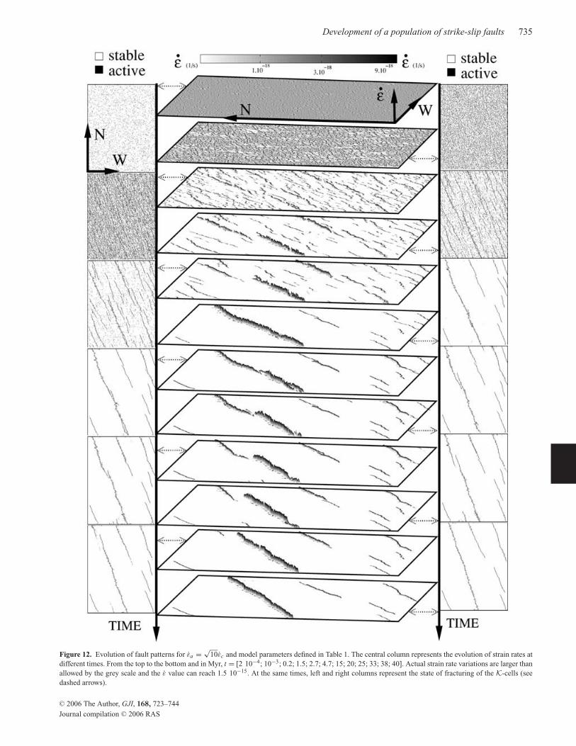
Figure 12. Evolution of fault patterns for εa = √10εc and model parameters defined in Table 1. The central column represents the evolution of strain rates at
different times. From the top to the bottom and in Myr, t = [2 10−4; 10−3; 0.2; 1.5; 2.7; 4.7; 15; 20; 25; 33; 38; 40]. Actual strain rate variations are larger thanallowed by the grey scale and the ε value can reach 1.5 10−15. At the same times, left and right columns represent the state of fracturing of the K-cells (seedashed arrows).
C© 2006 The Author, GJI, 168, 723–744
Journal compilation C© 2006 RAS

736 C. Narteau
In essence, megafault geometry is irregular because it is an ar-rangement of segments that have evolved under various configura-tions. In Fig. 12, it is possible to distinguish three major segmentsafter the megafault has been formed: two parallel southern segmentsare separated by a bend; a northern segment is present with an align-ment closer to the north–south direction than the alignment of thesouthern segments. These bends and irregularities in the alignmentof the fault are associated with low strain rates. This means that,in these areas, the localization process has not been achieved andthat the strain is distributed over a larger area. Zones where majorsegments connect are unstable while the fracturing process is stillintense. At the bend between the southern segments, it is possibleto distinguish the development of parallel segments from structuraldisorder. The new fault segments correspond to branches which,if they are stable in time, better satisfy the tectonic loading andthe local geometry of the fault network. In Fig. 12, the branch-ing phenomena is first observed along the southern segment. Theold branch becomes quickly inactive and concentration of strain isfavoured on the new branch. During this process, strain rates parti-tion along each branch of the fault. Later, a new branch also devel-ops towards the north along the central segment but its propagationis slower. In practice, the new branch competes with the previousone. Because the strain rates along these structures are high, nei-ther branch is dominant. The strain rate perturbations associatedwith their developments are not strong enough. This competitionlasts for a long time, and the strain rates along each fault fluctu-ate. Finally, the new branch dominates the system because of itsbetter alignment and propagates rapidly. The orientation of the newfault is more regular and bends have disappeared. The branchingphase erases the irregularity of the fault network with respect to theorientation of the tectonic loading. This may explain why maturefaults appear to be smooth along their strike and such a sharp dis-continuity perpendicularly to their strike. Since its formation, theevolution of the megafault has consisted of a clockwise rotation of itsalignment.
During the evolution of this network, a pull-apart disappears onthe major fault located at the north, two faults coalesce at the north-east corner, and two major faults compete with each other at thesoutheast corner. The youngest fault network presented in Fig. 12is extremely stable. It does not change for at least the next 100 My,i.e. over a timescale comparable with the lifetime of the present-dayplate-tectonic motions (DeMets et al. 1994).
3.2 General properties of the evolution of a populationof faults
In this section, emergent properties of the model are discussed.These properties result solely from the pattern of interaction betweenthe element of the system over long times because no pre-existingmaterial heterogeneities are determined a priori.
3.2.1 The localization process
Over different stages of development of a fault population, Fig. 13illustrates the localization process by showing the spatial distribu-tion of the transitions from stable to active along a transect lineperpendicular to the main direction and passing through the centreof the lattice.
From the nucleation to the branching phase, the deformation tendsto concentrate on larger and larger faults. These faults extend intotheir process zones and impede the development of other faultsin their neighbourhoods. Because strain rates are higher on pre-
0 150 250
0.25
0.75
1
Distance (K cell)
Act
ivat
ion
dens
ity
250 150 0 150 250
0.25
0.75
1
Distance (K cell)
Act
ivat
ion
dens
ity
250 150 0 150 250
0.25
0.75
1
Distance (K cell)
Act
ivat
ion
dens
ity
(a)
(b)
(c)
Figure 13. For the simulation presented on Fig. 8, the activation densityis plotted over three different time intervals: (a) nucleation phase (0 < t <
2 Myr), (b) growth phase (2 < t < 12 Myr) and (c) concentration phase(50 < t < 60 Myr). The activation density is the normalized distribution ofthe transitions from stable to active along a transect line perpendicular to theorientation of the megafault and passing by the centre of the lattice.
fractured (or weak) material, the faults accumulate the deformation,extend through increasingly larger areas which, in turn, participateto increase the strain rates along this structure. Consequently, local-ization is irreversible under constant loading.
The phenomenon of localization of deformation is a ubiquitousproperty of all the models of granular media and of brittle materi-als that combine elastic material properties and inelastic behaviourobserved in laboratory experiments (i.e. strain-hardening followedstrain-softening towards dynamic stress drop). The present modelembodies the same physical ideas and the localization results fromthe interplay between the anisotropy of the redistribution mecha-nism (elastic) and the local constitutive rule of evolution betweentwo different states of fracturing (plastic).
As shown by Cowie et al. (1993), Miltenberger et al. (1993) andSornette et al. (1994), the localization may be obtained by a self-organizing process towards a global state corresponding to a globalthreshold of effective plasticity. Without weakening, this requiresstrongly heterogeneous material properties which, in their model,predetermine the geometry of the fault population through all thestages of development. Deformation is concentrated on the ‘perco-lation backbone’, corresponding to the weakest line of elements ina particular direction. This paper confirms once more the impor-tance of heterogeneity but a distinction is that they are only incor-porated at a microscopic scale via statistical fluctuations. Thus, pre-existing material properties do not affect the evolution of the fault
C© 2006 The Author, GJI, 168, 723–744
Journal compilation C© 2006 RAS

Development of a population of strike-slip faults 737
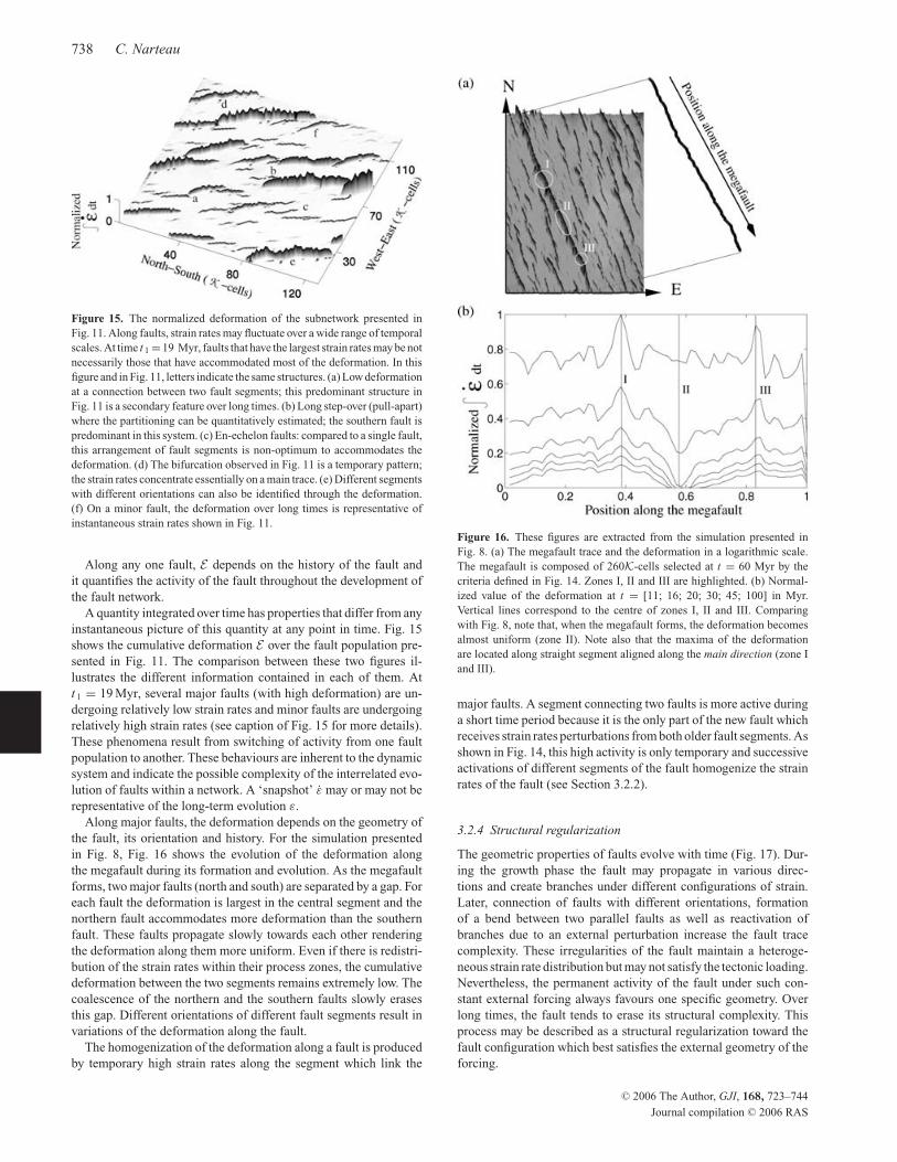
Figure 14. These figures are extracted from the simulation presented in Fig. 12. (a) The megafault trace. It is composed of 186K-cells selected at t = 18 Myrfrom a criteria: a cell is selected if, when it becomes active, (1) it is included in a fault of at least 200K-cells and (2) at least one cell of the length scale K+0.75Lbecomes active. (b) Evolution of the normalized strain rates along the megafault trace. Homogenization of strain rates follows the formation of the megafault.Note that this homogenization exists also on the southern and the northern segments before the formation of the central segment. The southern segment is moreactive than the northern one. It is possible to associate the main fluctuation of strain rates with structural irregularities. (c) The total strain rates measured alongthe megafault trace versus time.
populations in the model presented here. Therefore, the developmentof the geometry of the fault traces over long times is determined onlyby the redistribution mechanism. In this way, long-term behavioursare more easily extracted from the output of the model and are shownto be independent of the type of heterogeneity.
3.2.2 Homogenization of strain rates along megafaults
When faults grow, coalesce or interact, the strain rates along themvary. While faults are active, a homogenization of strain rates alongthese faults is observed. Fig. 14 shows the evolution of the strain ratesalong the primitive megafault presented in Fig. 12. Immediately fol-lowing the formation of the fault, the strain rates are uniform alongthe fault (Fig. 14b) except at major bends. The variation of the totalstrain rate along the megafault (Fig. 14c) increases monotonouslyalthough through a succession of plateaux. At t = 8.2 Myr, the to-tal strain rate along the megafault begins to decrease. The plateaux
and the increasing phases are explained by the growth and the co-alescence of different fault segments. The decrease indicates theimperfect orientation of the fault with respect to tectonic loadingand that the fault is slowly evolving towards a different configura-tion by branching (see Section 3.1.6).
Under a spatially uniform forcing, the homogenization of thestrain rates along the megafaults is regarded as a smoothing processwhich comes from the relationship between the strain rates and thetransition rates (see eqs 2 and 3). In fact, fault segments with largerstrain rates are activated more often and redistribute more energyonto neighbouring segments.
3.2.3 Evolution of the deformation along faults
For every K-cell at any time, the cumulative deformation is
E(x, y, t) =∫ t
0ε(x, y, τ ) dτ. (12)
C© 2006 The Author, GJI, 168, 723–744
Journal compilation C© 2006 RAS
738 C. Narteau
Figure 15. The normalized deformation of the subnetwork presented inFig. 11. Along faults, strain rates may fluctuate over a wide range of temporalscales. At time t 1 =19 Myr, faults that have the largest strain rates may be notnecessarily those that have accommodated most of the deformation. In thisfigure and in Fig. 11, letters indicate the same structures. (a) Low deformationat a connection between two fault segments; this predominant structure inFig. 11 is a secondary feature over long times. (b) Long step-over (pull-apart)where the partitioning can be quantitatively estimated; the southern fault ispredominant in this system. (c) En-echelon faults: compared to a single fault,this arrangement of fault segments is non-optimum to accommodates thedeformation. (d) The bifurcation observed in Fig. 11 is a temporary pattern;the strain rates concentrate essentially on a main trace. (e) Different segmentswith different orientations can also be identified through the deformation.(f) On a minor fault, the deformation over long times is representative ofinstantaneous strain rates shown in Fig. 11.
Along any one fault, E depends on the history of the fault andit quantifies the activity of the fault throughout the development ofthe fault network.
A quantity integrated over time has properties that differ from anyinstantaneous picture of this quantity at any point in time. Fig. 15shows the cumulative deformation E over the fault population pre-sented in Fig. 11. The comparison between these two figures il-lustrates the different information contained in each of them. Att 1 = 19 Myr, several major faults (with high deformation) are un-dergoing relatively low strain rates and minor faults are undergoingrelatively high strain rates (see caption of Fig. 15 for more details).These phenomena result from switching of activity from one faultpopulation to another. These behaviours are inherent to the dynamicsystem and indicate the possible complexity of the interrelated evo-lution of faults within a network. A ‘snapshot’ ε may or may not berepresentative of the long-term evolution ε.
Along major faults, the deformation depends on the geometry ofthe fault, its orientation and history. For the simulation presentedin Fig. 8, Fig. 16 shows the evolution of the deformation alongthe megafault during its formation and evolution. As the megafaultforms, two major faults (north and south) are separated by a gap. Foreach fault the deformation is largest in the central segment and thenorthern fault accommodates more deformation than the southernfault. These faults propagate slowly towards each other renderingthe deformation along them more uniform. Even if there is redistri-bution of the strain rates within their process zones, the cumulativedeformation between the two segments remains extremely low. Thecoalescence of the northern and the southern faults slowly erasesthis gap. Different orientations of different fault segments result invariations of the deformation along the fault.
The homogenization of the deformation along a fault is producedby temporary high strain rates along the segment which link the
Figure 16. These figures are extracted from the simulation presented inFig. 8. (a) The megafault trace and the deformation in a logarithmic scale.The megafault is composed of 260K-cells selected at t = 60 Myr by thecriteria defined in Fig. 14. Zones I, II and III are highlighted. (b) Normal-ized value of the deformation at t = [11; 16; 20; 30; 45; 100] in Myr.Vertical lines correspond to the centre of zones I, II and III. Comparingwith Fig. 8, note that, when the megafault forms, the deformation becomesalmost uniform (zone II). Note also that the maxima of the deformationare located along straight segment aligned along the main direction (zone Iand III).
major faults. A segment connecting two faults is more active duringa short time period because it is the only part of the new fault whichreceives strain rates perturbations from both older fault segments. Asshown in Fig. 14, this high activity is only temporary and successiveactivations of different segments of the fault homogenize the strainrates of the fault (see Section 3.2.2).
3.2.4 Structural regularization
The geometric properties of faults evolve with time (Fig. 17). Dur-ing the growth phase the fault may propagate in various direc-tions and create branches under different configurations of strain.Later, connection of faults with different orientations, formationof a bend between two parallel faults as well as reactivation ofbranches due to an external perturbation increase the fault tracecomplexity. These irregularities of the fault maintain a heteroge-neous strain rate distribution but may not satisfy the tectonic loading.Nevertheless, the permanent activity of the fault under such con-stant external forcing always favours one specific geometry. Overlong times, the fault tends to erase its structural complexity. Thisprocess may be described as a structural regularization toward thefault configuration which best satisfies the external geometry of theforcing.
C© 2006 The Author, GJI, 168, 723–744
Journal compilation C© 2006 RAS

Development of a population of strike-slip faults 739
102
103
104
105
106
107
108
0.7
0.9
1
Time (years)
< n
F /
l F >
I
II
IIIFa
ults
com
plex
ity
Figure 17. Temporal variation of the complexity of the fault traces. Av-eraged on 100 consecutive transitions from a stable to an active state, thismeasure of the fault complexity is the normalized ratio between the numberof K-cells included in a fault and the length of this fault. The lower the valueof this parameter is, the more regular the fault traces are. This figure is ob-tained from the simulation presented in Fig. 12. Three periods are indicated.Period I: creation of the faults by nucleation, growth and coalescence. Thecomplexity of the trace increases until it reach a maximum value. Period II:fault interaction and beginning of the concentration of strain rates. The com-plexity stay almost constant because while some faults continue to develop,the trace of older ones become more regular. Period III: branching phase andmegafault evolution. The complexity decreases rapidly to converge towardsan asymptotic value.
For the range of parameters presented in this paper, the branchingphase may be treated as a subprocess of the structural regularizationbecause it favours a specific orientation of the fault with respect tothe tectonic loading.
3.2.5 Evolution of strain rates per unit of fault length
The averaged strain rate along the fault is an important property indetermining the activity of the fault. For each fault, the evolution ofthe averaged strain rate may give important indications regarding thefuture evolution of the network. The relation between the strain rateper unit of fault length versus the length of the fault is presented inFig. 18. Depending on the length of the fault, three types of variationsare observed. Small faults of length lF < 0.2L concentrate lowstrain rates because they do not interact with other faults. Thesestrain rates per unit of fault length increase relatively slowly withlength of fault. Faults with lengths ranging from lF = 0.2L tolF = 0.7L interact with other faults and concentrate higher strainrates. These strain rates per unit of fault length increase more rapidlythan during the growth phase. The megafault lF > 0.7L does notaccumulate higher strain rates per unit of fault length because itresults from the coalescence of major faults which have alreadyconcentrated all the deformation.
4 D I S C U S S I O N
Starting with a completely homogeneous system, the time-dependent stochastic process outlined in this paper succeeds inreproducing important characteristics of the development of faultsystems. Progress in computer power and more precise knowledge
60 120 180 240 300
0.25
0.75
1
K
(nor
mal
ized
)
per
unit
of f
ault
leng
thA
vera
ge s
trai
n ra
te
Figure 18. The averaged strain rate per unit of fault length versus the lengthof the fault. The y-axis is the normalized ratio between the sum of strain ratesalong the faults and the number ofK-cells composing these faults. This figureis obtained from the simulation presented in Fig. 12. For three fault lengthintervals, dotted segments indicate linear trends corresponding to differentphases of development: l F ∈ [0; 70], small faults are observed during thenucleation and growth phases; they do not interact with neighbouring faultsand concentrate few strain rates. l F ∈ [70; 180], major fault formation isobserved during the interaction and the concentration phases; they interactwith other fault and accommodate more efficiently the deformation. l F >
180, a megafault resulting from the coalescence of major faults is observed;this fault had already concentrated all the strain rates along them and nochange of the strain rates density is observed when they coalesce. The plateaucorresponds to the amplitude of the external forcing (∼ εa).
of the crust may perhaps allow incorporation of all types of hetero-geneities and the validation of elastodynamic laws under geophys-ical conditions. Until that time, it is important to provide a generalexplanation of how a large number of behaviours can be derivedfrom a small number of physical ingredients. In this study, het-erogeneities are required to justify the stochastic process. The keypoint is that these heterogeneities are not predetermined. In fact, thesystem itself converges towards a stationary statistical state whichdoes not depend on pre-existing material properties. Once this sta-tionary statistical state systematically emerges, characteristic spatialand temporal behaviours related to a whole class of self-organizedcomplex systems can be extracted (e.g. localization, structural reg-ularization, distribution of both strain rates and deformation alongfaults).
The model shows that when fault growth produces bends, ir-regularities and different types of unstable configurations betweendifferent fault segments, the fault traces may evolve towards anotherconfiguration. This evolution implies a partitioning of the strain ratesand a competition between parallel branches of the same fault. Inthe end, the branch with better interactions dominates the other. Inthis paper, this branching phase has been described at the largestscale of the fault system. In geophysical systems, such internal evo-lutionary mechanisms may exist. Interestingly, it only requires faultinteractions and may occur without rotational conditions or exter-nal modifications of the external forcing. In particular, the branchingphase offers new perspectives for the modelling of different typesof fracture if no quasi-stable configuration can be reached.
Furthermore, the branching phase illustrates an advantage of atime-dependent stochastic approach with uniform material proper-ties. Such a branching mechanism consists of a complete relocationof largest scale faults with either the removal or the formation of
C© 2006 The Author, GJI, 168, 723–744
Journal compilation C© 2006 RAS

740 C. Narteau
new bends or irregularities along their traces. It may be describedas a relocalization of the deformation by reorganization. In a modelwith heterogeneous failure thresholds, such a behaviour can notbe reproduced without an additional strengthening process becausethe configurations associated with the global threshold of effec-tive plasticity impede a complete relocation of the predominantfaults. Then, the final geometry of faults in mechanically hetero-geneous model is an optimal interface structure (the percolation‘backbone’) which can be determined a priori from the spatial dis-tribution of the material properties (Sornette et al. 1994). Here,without any pre-determined heterogeneity, the geometries and theorientations of the megafaults are determined by the rules of in-teraction and the shape of the redistribution. These faults can belocated anywhere in response to the statistical fluctuations asso-ciated with the time-dependent stochastic process and the limita-tions imposed by the boundary conditions. Furthermore, the faulttraces do not always converge automatically towards an ideal con-figuration, and can sequentially display different unstable configu-rations. Such configurations are equiprobable and when the strainrates have transitioned from one fault to another, except by chance,there is no reason for the same fault configuration to become activeagain.
While the branching phase modifies the largest scale of a faultsystem, structural regularization is a similar mechanism occurringat smaller scales. Bends, turns and branches of the fault traces maydisappear with respect to a smoothing process which, over longtimes, results from the anisotropy of the redistribution mechanismvia the accumulation of the deformation (Wesnousky 1988). Suchan observation is difficult to extract from a model with pre-existingmaterial heterogeneities. In fact, the structural regularization canconflict with the optimization process of the fault path. In the presentmodel, because the optimal fault path is a straight line orientedwith respect to the tectonic loading, any convergence towards thisstate can be more easily observed and associated with the structuralregularization process.
Material properties which incorporate pre-existing hetero-geneities and time-dependent rheologies (weakening or strength-ening) are not in contradiction with the stochastic approach. Suchadditional ingredients can easily be introduced into the modellingif required. For now, it is important to have demonstrated that struc-tural regularization does not require a pre-existing heterogeneity.
A particularity of the model is that the overlap to separation ra-tio between neighbouring faults is taken into account through theimplementation of a geometric interaction criterion at increasinglylarger scales of a multiscale system. Thus, in addition to long rangeinteractions, the evolution of the populations of faults also dependon short range interactions between faults situated near to one an-other. Intuitive rules based on observations and fracture mechanicssuch as those suggested in this paper have to be tested. They re-produce the same basic behaviours as any other reasonable rulesimitating the same phenomena. The purpose is to develop a sys-tem in which it is possible to analyse complexity through a lim-ited number of parameters. This practical approach complementstraditional ones and offers the possibility of discussing the evolutionof geophysical systems over a wide range of temporal and spatialscales.
This paper focuses on the properties of fault populations as wellas on the properties of any fault within these fault populations. Atany time, it is possible to describe how the strain rates are dis-tributed over different faults. These tectonic rates, integrated overdifferent time intervals, determine the deformation along the faultson different timescales. Instantaneous and integrated pictures of the
system could be compared to geodetic and geological observationswithin active tectonic regions. If such variations in strain rates existalong real faults, it is important to consider them for time depen-dant assessment of earthquake hazards. The model presented herecan propose and classify these interpretations from the structuralpatterns observed in a population of strike-slip faults. Simultane-ously, its predictions could be used to look for new observations innatural exposures.
In the present model, it is possible to analyse the competitionbetween faults via the partition of the strain rates but not via thetemporal distribution of earthquakes (Lee et al. 1999). In fact, onlythe distribution of strain rates over a population of interacting faultshas been taken into account. Future work will concentrate on seis-mic patterns at different stages of the evolution of a populationof faults. The idea is to develop a general model that couples aprevious model of seismicity presented in Narteau (2006) and themodel of development of a fault population presented in this pa-per. Interestingly, they complement each other and could togetherprovide a global description of the spatial-temporal properties ofstress dissipation within a crustal shear zone. In a general seismo-tectonic model, instead of considering a homogeneous loading andheterogeneous failure threshold, the present model will allow theintroduction of heterogeneous loading rates which result from faultinteractions at all stages of the development of a population offaults.
In Narteau (2006), at the length scale K of a fault segment, it ispossible to relate different seismic behaviours of a fault zone withthe magnitude of a non-dimensional parameter A. This parameter isthe ratio between the loading rate and the product of the healing rateand the local stress drop. If A ≈ 1, the system is in a critical stateand large events can occur over a wide range of temporal scales; ifA < 1, the system is in a subcritical state controlled by faulting andseismic precursors are frequently observed; if A > 1, the systemis in a subcritical state controlled by healing and the fault zonemay be creeping. One particular feature is that the magnitude of thestress stored in the fault zone decreases and the proportion of largeevents increases as the critical point is approached. This has beeninterpreted as a weakening process.
If the healing rate and the local stress drop are assumed to have aconstant and uniform value, the strain rate used in the present modelwill be proportional to the parameter A used in Narteau (2006). Inthis case, from the results of both models, it is possible to infer ageneral scenario and to conclude the following.
The increase in fault dimension enables the propagation of largerearthquakes. Consequently, over the development of fault popula-tions such as presented in this paper, increasingly larger events can beexpected. Moreover, because fault segments under a critical regime(i.e. A ≈ 1) have a greater proportion of large ruptures, neighbouringfault segments may become critical as following.
(i) Along segments with A > 1, it is because large and discon-tinuous stress dissipations may temporally favour the strengthening,and, so, produce a delayed but significant seismic activity.
(ii) Along segments with A < 1, it is because the slip may bedirectly triggered by stress perturbations associated with the rupturefront propagation along an adjacent segments.
Finally, if some parts of the fault are in a critical state, the seismicregime of the entire fault network may become critical. Then, theweakening process observed at the length scale of a fault segmentis likely to occur at larger length scales. Such, a weakening processaccelerates localization of the deformation along pre-existing faultswhich tends to grow (see the beginning of the paragraph).
C© 2006 The Author, GJI, 168, 723–744
Journal compilation C© 2006 RAS
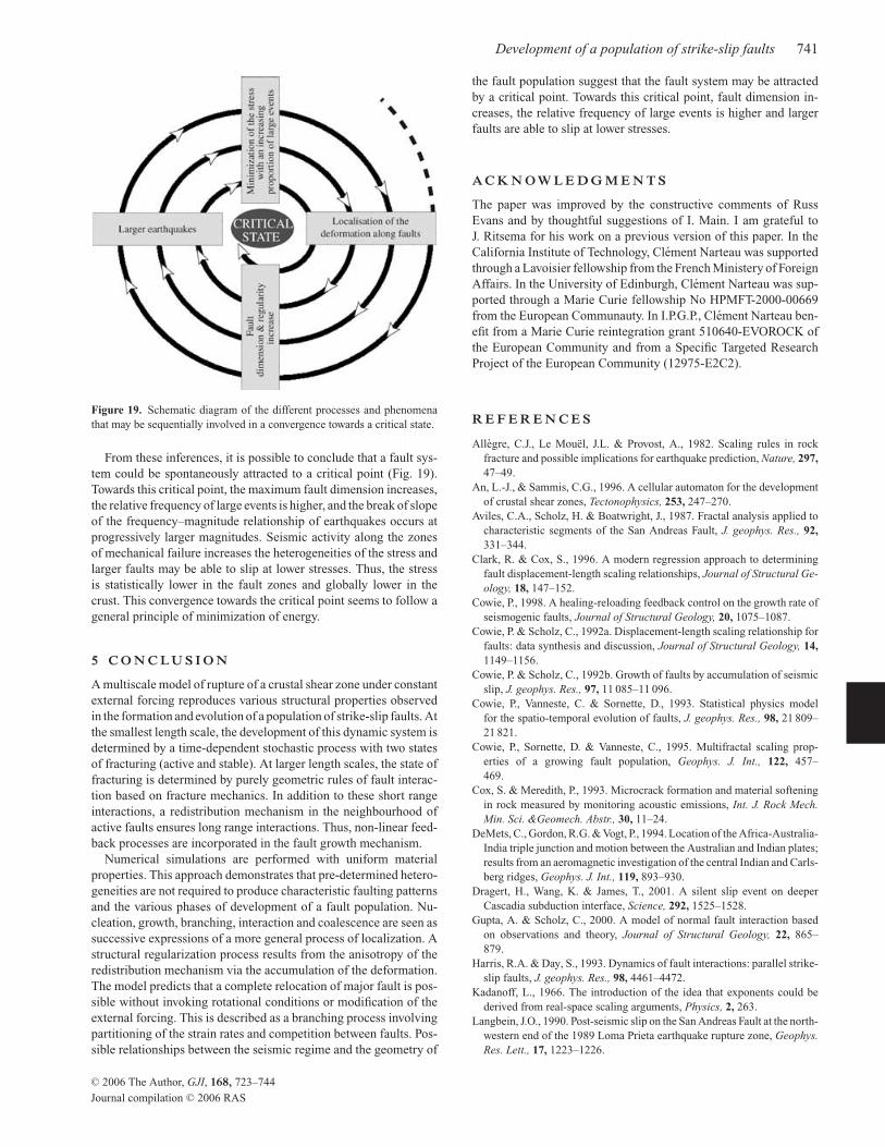
Development of a population of strike-slip faults 741
Figure 19. Schematic diagram of the different processes and phenomenathat may be sequentially involved in a convergence towards a critical state.
From these inferences, it is possible to conclude that a fault sys-tem could be spontaneously attracted to a critical point (Fig. 19).Towards this critical point, the maximum fault dimension increases,the relative frequency of large events is higher, and the break of slopeof the frequency–magnitude relationship of earthquakes occurs atprogressively larger magnitudes. Seismic activity along the zonesof mechanical failure increases the heterogeneities of the stress andlarger faults may be able to slip at lower stresses. Thus, the stressis statistically lower in the fault zones and globally lower in thecrust. This convergence towards the critical point seems to follow ageneral principle of minimization of energy.
5 C O N C L U S I O N
A multiscale model of rupture of a crustal shear zone under constantexternal forcing reproduces various structural properties observedin the formation and evolution of a population of strike-slip faults. Atthe smallest length scale, the development of this dynamic system isdetermined by a time-dependent stochastic process with two statesof fracturing (active and stable). At larger length scales, the state offracturing is determined by purely geometric rules of fault interac-tion based on fracture mechanics. In addition to these short rangeinteractions, a redistribution mechanism in the neighbourhood ofactive faults ensures long range interactions. Thus, non-linear feed-back processes are incorporated in the fault growth mechanism.
Numerical simulations are performed with uniform materialproperties. This approach demonstrates that pre-determined hetero-geneities are not required to produce characteristic faulting patternsand the various phases of development of a fault population. Nu-cleation, growth, branching, interaction and coalescence are seen assuccessive expressions of a more general process of localization. Astructural regularization process results from the anisotropy of theredistribution mechanism via the accumulation of the deformation.The model predicts that a complete relocation of major fault is pos-sible without invoking rotational conditions or modification of theexternal forcing. This is described as a branching process involvingpartitioning of the strain rates and competition between faults. Pos-sible relationships between the seismic regime and the geometry of
the fault population suggest that the fault system may be attractedby a critical point. Towards this critical point, fault dimension in-creases, the relative frequency of large events is higher and largerfaults are able to slip at lower stresses.
A C K N O W L E D G M E N T S
The paper was improved by the constructive comments of RussEvans and by thoughtful suggestions of I. Main. I am grateful toJ. Ritsema for his work on a previous version of this paper. In theCalifornia Institute of Technology, Clement Narteau was supportedthrough a Lavoisier fellowship from the French Ministery of ForeignAffairs. In the University of Edinburgh, Clement Narteau was sup-ported through a Marie Curie fellowship No HPMFT-2000-00669from the European Communauty. In I.P.G.P., Clement Narteau ben-efit from a Marie Curie reintegration grant 510640-EVOROCK ofthe European Community and from a Specific Targeted ResearchProject of the European Community (12975-E2C2).
R E F E R E N C E S
Allegre, C.J., Le Mouel, J.L. & Provost, A., 1982. Scaling rules in rockfracture and possible implications for earthquake prediction, Nature, 297,47–49.
An, L.-J., & Sammis, C.G., 1996. A cellular automaton for the developmentof crustal shear zones, Tectonophysics, 253, 247–270.
Aviles, C.A., Scholz, H. & Boatwright, J., 1987. Fractal analysis applied tocharacteristic segments of the San Andreas Fault, J. geophys. Res., 92,331–344.
Clark, R. & Cox, S., 1996. A modern regression approach to determiningfault displacement-length scaling relationships, Journal of Structural Ge-ology, 18, 147–152.
Cowie, P., 1998. A healing-reloading feedback control on the growth rate ofseismogenic faults, Journal of Structural Geology, 20, 1075–1087.
Cowie, P. & Scholz, C., 1992a. Displacement-length scaling relationship forfaults: data synthesis and discussion, Journal of Structural Geology, 14,1149–1156.
Cowie, P. & Scholz, C., 1992b. Growth of faults by accumulation of seismicslip, J. geophys. Res., 97, 11 085–11 096.
Cowie, P., Vanneste, C. & Sornette, D., 1993. Statistical physics modelfor the spatio-temporal evolution of faults, J. geophys. Res., 98, 21 809–21 821.
Cowie, P., Sornette, D. & Vanneste, C., 1995. Multifractal scaling prop-erties of a growing fault population, Geophys. J. Int., 122, 457–469.
Cox, S. & Meredith, P., 1993. Microcrack formation and material softeningin rock measured by monitoring acoustic emissions, Int. J. Rock Mech.Min. Sci. &Geomech. Abstr., 30, 11–24.
DeMets, C., Gordon, R.G. & Vogt, P., 1994. Location of the Africa-Australia-India triple junction and motion between the Australian and Indian plates;results from an aeromagnetic investigation of the central Indian and Carls-berg ridges, Geophys. J. Int., 119, 893–930.
Dragert, H., Wang, K. & James, T., 2001. A silent slip event on deeperCascadia subduction interface, Science, 292, 1525–1528.
Gupta, A. & Scholz, C., 2000. A model of normal fault interaction basedon observations and theory, Journal of Structural Geology, 22, 865–879.
Harris, R.A. & Day, S., 1993. Dynamics of fault interactions: parallel strike-slip faults, J. geophys. Res., 98, 4461–4472.
Kadanoff, L., 1966. The introduction of the idea that exponents could bederived from real-space scaling arguments, Physics, 2, 263.
Langbein, J.O., 1990. Post-seismic slip on the San Andreas Fault at the north-western end of the 1989 Loma Prieta earthquake rupture zone, Geophys.Res. Lett., 17, 1223–1226.
C© 2006 The Author, GJI, 168, 723–744
Journal compilation C© 2006 RAS

742 C. Narteau
Lee, M.W., Sornette, D. & Knopoff, L., 1999. Persistence and quies-cence of seismicity on fault systems, Phys. Rev. Lett., 20, 4219–4222.
Mandl, G., 2000. Faulting in brittle rocks, Springer.Manighetti, I., King, G., Gaudemer, Y., Scholz, C. & Doubre, C., 2001. Slip
accumulation and lateral propagation of active normal fault in Afar, J.geophys. Res., 106, 13 667–13 696.
Mann, P., Hempton, M. & Dwight, C., 1983. Development of pull-apartbasins, J. Geol., 91, 529–554.
Miltenberger, P., Sornette, D. & Vanneste, C., 1993. Fault self-organizationas optimal random paths selected by critical spatio-temporal dynamics ofearthquakes, Phys. Rev. Lett., 71, 3604–3607.
Narteau, C., 2006. Classification of seismic patterns in a hierarchicalmodel of rupture: a new phase diagram for seismicity, Geophys. J. Int.,doi:10.1111/j.1365-246X.2006.03212.x.
Narteau, C., Shebalin, P., Holschneider, M., Le Mouel, J.L. & Allegre, C.J.,2000. Direct simulation of the stress redistribution in the scaling organi-zation of fracture tectonics, Geophys. J. Int., 141, 115–135.
Narteau, C., Le Mouel, J.-L., Poirier, J., Sepulveda, E. & Shnirman, M.G.,2001. On a small scale roughness of the core-mantle boundary, Phys.Earth planet. Int., 191, 49–61.
Peacock, D. & Sanderson, D.J., 1991. Displacement, segment linkage andrelay ramps in normal fault zones, Journal of Structural Geology, 13,721–731.
Reynolds, P., Klein, W. & Stanley, H., 1977. Renormalization group for siteand bond percolation, Phys. C, 10, 167–172.
Rockwell, T., Lindvall, S., Herzberg, M., Murbach, D., Dawson, T. & Berger,G., 2000. Paleoseismology of the Johnson Valley, Kickapoo, and Home-stead Valley faults, Bull. seism. Soc. Am., 90, 1200–1236.
Rodgers, D., 1980. Analysis of pull-apart basin development produced byen-enchelon strike-slip faults, Special publication of the I.A. of Sedimen-tologists, 4, 27–41.
Schlische, R., Young, S., Ackerman, R. & Gupta, A., 1996. Geometry andscaling relations of a population of very small rift related normal faults,Geology, 24, 683–686.
Simpson, R.W., Lienkaemper, J.J. & Galehouse, J.S., 2001. Variations increep rate along the Hayward Fault, California, interpreted as changes indepth of creep, Geophys. Res. Lett., 28, 2269–2272.
Sornette, D., Miltenberger, P. & Vanneste, C., 1994. Statistical physics offault patterns self-organized by repeated earthquakes, Pure appl. Geo-phys., 142, 491–527.
Turcotte, D.L., 1997. Fractals and Chaos in Geology and Geophysics,Cambridge University Press, Cambridge.
Van der Woerd, J. et al., 2000. Uniform slip-rate along the Kunlun Fault:implications for seismic behaviour and large-scale tectonics, Geophys.Res. Lett., 27, 2353–2356.
Wesnousky, S., 1988. Seismological and structural evolution of strike-slipfaults, Nature, 335, 340–343.
A P P E N D I X A : T H E M A S K S
The six masks used in the redistribution of the strain rates are
M N{m,a,b}(x, y) =
m∑i=1
1
i2
(QN
1 ξ a+i−1a−i+1 (x)ξ b−i
b−i (y) + ξ a−ia−i (x)
(QN
2 ξ b−1b−i (y)
+ QN3 ξ b+i−1
b (y) + QN4 ξ b+2i−1
b+i (y)))
,
(A1)
MNW{m,a,b}(x, y) =
m∑i=1
1
i2
(ξ b−i
b−i (y)(QNW
1 ξ a−1a−i+1(x) + QNW
2 ξ a+i−1a (x) + QNW
3 ξ a+2i−1a+i (x)
)+ ξ a−i
a−i (x)(QNW
1 ξ b−1b−i (y) + QNW
4 ξ b+i−1b (y) + QNW
3 ξ b+2i−1b+i (y)
)),
(A2)
MW{m,a,b}(x, y) =
m∑i=1
1
i2
(QW
1 ξ a−ia−i (x)ξ b+i−1
b−i+1 (y)
+ ξ b−ib−i (y)
(QW
2 ξ a−1a−i (x) + QW
3 ξ a+i−1a (x) + QW
4 ξ a+2i−1a+i (x)
)),
(A3)
M S{m,a,b}(x, y) =
m∑i=1
1
i2
(QS
1ξa+i−1a−i+1 (x)ξ b+i
b+i (y) + ξ a+ia+i (x)
(QS
2ξb−ib−2i+1(y)
+ QS3ξ
bb−i+1(y) + QS
4ξb+ib+1(y)
)),
(A4)
MSE{m,a,b}(x, y) =
m∑i=1
1
i2
(ξ b+i
b+i (y)(QSE
1 ξ a+i−1a+1 (x) + QSE
2 ξ aa−i+1(x) + QSE
3 ξ a−ia−2i+2(x)
)+ ξ a+i
a+i (x)(QSE
3 ξ b−ib−2i+2(y) + QSE
4 ξ bb−i+1(y) + QSE
1 ξ b+ib+1(y)
)),
(A5)
M E{m,a,b}(x, y) =
m∑i=1
1
i2
(QE
1 ξ a+ia+i (x)ξ b+i−1
b−i+1 (y)
+ ξ b+ib+i (y)
(QE
2 ξ a+ia+1(x) + QE
3 ξ aa−i+1(x) + QE
4 ξ a−ia−2i+1(x)
)),
(A6)
with
ξvu (w) =
{1 if w ∈ [u, v] with 0 < u ≤ v,
0 otherwise,
and Qdi , d ∈ {N, NW, W, S, SE, E}, i ∈ {1, 2, 3, 4}, parameters defined in Fig. 6.
C© 2006 The Author, GJI, 168, 723–744
Journal compilation C© 2006 RAS

Development of a population of strike-slip faults 743
A P P E N D I X B : S T R A I N R A T E R E D I S T R I B U T I O N
The total strain rates perturbation mask is
ϒ(x, y) = ρεa
√km
∑o∈CK
F
∑p∈{N ,...,E}
M p
{e po ,xo,yo}(x, y) (B1)
with ρ a constant, εa the amplitude of the external forcing, CKF the elementary cells composing the fault F, and (x o, yo) the coordinates of
the o-cell in the 2-D lattice.The total stress rate perturbation mask may be decomposed into a process zone mask and a shadow zone mask:
ϒ(x, y) = ϒP (x, y)︸ ︷︷ ︸process zones
+ ϒS (x, y)︸ ︷︷ ︸shadow zones
(B2)
with,
ϒP (x, y) ={
ϒ(x, y) if ϒ(x, y) > 0,
0 otherwise,(B3)
and,
ϒS (x, y) ={
0 if ϒ(x, y) > 0,
ϒ(x, y) otherwise.(B4)
Furthermore, the process zones mask may be decomposed in a active and stable process zones mask:
ϒP (x, y) = ϒaP (x, y)︸ ︷︷ ︸active
+ ϒ sP (x, y)︸ ︷︷ ︸stable
(B5)
with,
ϒaP (x, y) =
{ϒP (x, y) if CK
(x,y) is active,
0 otherwise,(B6)
and,
ϒ sP (x, y) =
{ϒP (x, y) if CK
(x,y) is stable,
0 otherwise.(B7)
The maximum strain rates added to active and stable cells of the elementary scale are respectively
RaP =
L∑x=1
L∑y=1
ϒaP (x, y), (B8)
and,
RsP =
L∑x=1
L∑y=1
ϒ sP (x, y). (B9)
In practice, the shadow zone mask is applied first and ε(x, y) cannot be negative:
�S (x, y) = max (−ε(x, y), ϒS (x, y)) , (B10)
The amount of strain rate available for the process zone masks is
RS = −L∑
x=1
L∑y=1
�S (x, y). (B11)
These strain rates may be redistributed by first adding the active process zone mask:
�aP (x, y) = ϒa
P (x, y)
(1 − max
(0,
RaP − RS
RaP
)). (B12)
Second, the remaining strain rates
RS ′ = RS −L∑
x=1
L∑y=1
�aP (x, y) (B13)
are added to the stable process zone mask:
�sP (x, y) = ϒ s
P (x, y)
(1 − max
(0,
RsP − R′
SRsP
)). (B14)
C© 2006 The Author, GJI, 168, 723–744
Journal compilation C© 2006 RAS

744 C. Narteau
Then, the remaining strain rates
R′′S = R′
S −L∑
x=1
L∑y=1
�sP (x, y) (B15)
are finally redistributed uniformly on the fault:
�F (x, y) =
R′′S
nF (K)if CK
(x,y) ∈ CKF ,
0 otherwise,
(B16)
with nF (K) the total number of cells of the elementary scale composing the fault F.Thus the total strain rate redistribution is
�(x, y) = �S (x, y) + �aP (x, y) + �s
P (x, y) + �F (x, y) (B17)
C© 2006 The Author, GJI, 168, 723–744
Journal compilation C© 2006 RAS
Related Documents