Forensic Steganalysis: Determining the Stego Key in Spatial … · Forensic Steganalysis: Determining the Stego Key in Spatial Domain Steganography aJessica Fridrich∗, aMiroslav

Forensic Steganalysis: Determining the Stego Key in Spatial Domain Steganography

aJessica Fridrich∗, aMiroslav Goljan, bDavid Soukal, and aTaras Holotyak

aDept. of Electrical and Computer Engineering, bDept. of Computer Science

SUNY Binghamton, Binghamton, NY 13902-6000, USA

ABSTRACT

This paper is an extension of our work1 on stego key search for JPEG images published at EI SPIE in 2004. We provide a more general theoretical description of the methodology, apply our approach to the spatial domain, and add a method that determines the stego key from multiple images. We show that in the spatial domain the stego key search can be made significantly more efficient by working with the noise component of the image obtained using a denoising filter. The technique is tested on the LSB embedding paradigm and on a special case of embedding by noise adding (the ±1 embedding). The stego key search can be performed for a wide class of steganographic tech-niques even for sizes of secret message well below those detectable using known methods. The proposed strategy may prove useful to forensic analysts and law enforcement.

1. INTRODUCTION The art of discovering secret messages embedded using steganography2 is called steganalysis. The vast majority of work in steganalysis focuses on detection of secret messages rather than extraction. On a more general level, stega-nalysis comprises of several phases, some of which belong to digital forensic analysis (hence the term Forensic Steganalysis in the title of this paper): 1) identification of suspicious images, 2) determining the steganographic method in use, 3) searching for the stego key and extracting the embedded bit-stream, 4) deciphering the bit-stream. In this paper, we investigate Phase 3 under the assumption that we have one or more stego images and, by Kerck-hoffs’ principle, we already know the steganographic program used for embedding (i.e., we have the source code). One simple approach to determine the stego key would be to use a brute-force search for the stego key, inspecting the most likely keys first (dictionary attack) and extracting the alleged message while looking for a recognizable header as a sign that we have come across the correct stego key3. However, this approach will fail if the embedded data stream does not have any detectable structure in which case the search also becomes significantly more com-plicated because for each stego key, all possible encryption keys must be tested. Thus, the complexity of the brute force search is proportional to the product of the size of stego and encryption keyspaces. Even though for some stego programs the stego key space itself may be small enough to make the brute force search for the stego key plausible, if the message has been encrypted using strong encryption, the search becomes computationally infeasi-ble. Trivedi et al.4,5 presented a method for secret key detection in sequential steganography. The authors’ goal is to determine, using a sequential probability ratio test, the embedding key, which is, in their interpretation, the begin-ning and the end of the subsequence modulated during embedding. In contrast, in this paper the key determines a pseudo-randomly ordered subset of all indices in the cover signal to be used for embedding. This situation is more typical for a steganographic application, while sequential embedding is typically used for watermarking. While it is possible to apply the method of Ref. 4 for this case by performing the same hypothesis test for each possible key, additional research would have to be done to estimate the probability of falsely determined and missed keys. Also, the necessity to encounter a jump in the statistics implies that the whole signal used for embedding must be proc-essed, which would slow down the search. In this paper, we follow the approach previously proposed for JPEG images1 and modify it for spatial domain steg-anography. In the next section, we define the embedding paradigm that will be investigated in this paper and in Section 3 we give a detailed problem formulation. The stego key search method itself is described in Section 4. In ∗ [email protected]; phone 1 607 777-2577; fax 1 607 777-4464; http://www.ws.binghamton.edu/fridrich

Section 5, experimental results are interpreted and discussed for ±1 embedding and Least Significant Bit embed-ding (LSB) in the spatial domain. In Section 6, we show how the reliability of the search can be improved if multi-ple stego images embedded with the same key are available. Finally, the paper is concluded in Section 7 where we discuss limitations of the proposed method and possible countermeasures.

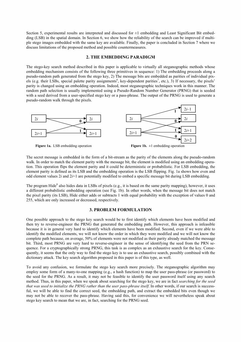
2. THE EMBEDDING PARADIGM The stego-key search method described in this paper is applicable to virtually all steganographic methods whose embedding mechanism consists of the following three primitives in sequence: 1) The embedding proceeds along a pseudo-random path generated from the stego key, 2) The message bits are embedded as parities of individual pix-els (e.g. their LSBs, special palette parity assignments6, key-dependent parities7, etc.), 3) If necessary, the pixels’ parity is changed using an embedding operation. Indeed, most steganographic techniques work in this manner. The random path selection is usually implemented using a Pseudo-Random Number Generator (PRNG) that is seeded with a seed derived from a user-specified stego key or a pass-phrase. The output of the PRNG is used to generate a pseudo-random walk through the pixels.

2i+1

2i 2i

2i+1

0

1 1

i

1

i

1

1

Figure 1a. LSB embedding operation

The secret message is embedded in the form of a bit-stream awalk. In order to match the element parity with the message btion. This operation flips the element parity and it could be delement parity is defined as its LSB and the embedding operaodd element values 2i and 2i+1 are potentially modified to em The program Hide8 also hides data in LSBs of pixels (e.g., it ia different probabilistic embedding operation (see Fig. 1b). Ithe pixel parity (its LSB), Hide either adds or subtracts 1 with255, which are only increased or decreased, respectively.

3. PROBLEM FOR One possible approach to the stego key search would be to fthen try to reverse-engineer the PRNG that generated the embecause it is in general very hard to identify which elements identify the modified elements, we will not know the order incomplete path because, on average, 50% of elements were notbit. Third, most PRNG are very hard to reverse-engineer inquence. For a cryptographically strong PRNG, this task is as quently, it seems that the only way to find the stego key is to dictionary attack. The key search algorithm proposed in this p To avoid any confusion, we formulate the stego key searchemploy some form of a many-to-one mapping (e.g., a hash futhe seed for the PRNG. As a result, it may not be feasible method. Thus, in this paper, when we speak about searching fthat was used to initialize the PRNG rather than the user passful, we will be able to find the correct seed, the embedding may not be able to recover the pass-phrase. Having said thistego key search to mean that we are, in fact, searching for the

2i+

2

Figure 1b. ±1 embedding operatio

0

s the parity of the elements alongit, the element is modified using aeterministic or probabilistic. For Ltion is the LSB flipping. Fig. 1a sbed a specific message bit during

s based on the same parity mappinn other words, when the message equal probability with the excep

MULATION

irst identify which elements havebedding path. However, this ap

have been modified. Second, eve which they were modified and w modified as their parity already m the sense of identifying the seedcomplex as an exhaustive searchuse an exhaustive search, possiblyaper is of this type, as well.

more precisely. The steganogranction) to map the user pass-phra

to identify the user password itseor the stego key, we are in fact se-phrase itself. In other words, if opath, and extract the embedded bs, for convenience we will never PRNG seed.

2i–

2

2i+

2

0

1

n

the pseudo-random n embedding opera-SB embedding, the

hows how even and LSB embedding.

g), however, it uses bit does not match tion of values 0 and

been modified and proach is infeasible n if we were able to e will not know the atched the message from the PRN se-

for the key. Conse- combined with the

phic algorithm may se (or password) to lf using any search arching for the seed ur search is success-its even though we theless speak about

Throughout this text, boldface symbols will denote vectors or matrices, non-boldface symbols will stand for scalars, and boldface Greek symbols will denote random variables. We reserve the letter i to index image elements, k for indices of histogram bins, and j to index stego keys. Let the cover image be represented with a vector x={xi}, i=1, …, N. Depending on the image format, the elements xi can be shades of gray or color indices. The range of xi is a finite set of integers. Let K be the space of all possible stego keys that lead to different pseudo-random paths. After embedding m message bits, the stego image, x(q) = {xi(q)}, is obtained, where q = m/N is the relative message length. During embedding, at least m≤N elements in x are visited (and potentially modified) along the path generated from the stego key K0∈K. Our task is to find the embedding stego key K0 given only the stego image x(q) and a full knowledge of the embedding algorithm. For each possible candidate key Kj∈K, let Path(Kj) denote the ordered set of element indices visited along the path generated from the key Kj. Assuming the embedded message bits are i.i.d. realizations of a binary random variable uniformly distributed on {0, 1} (which is the case if the message is encrypted), in the sequence {xi(q)}, i∈Path(K0), on average 50% of elements were modified by the embedding operation. Thus, taking the first n elements along the path generated from the correct key, n≤m, the expected number of modified elements is n/2. Assuming paths produced from different keys are independent and that each path of length n forms a random subset of the cover image (each element has the same probability of being selected), the probability of encountering a modified element is m/(2N). Thus, the expected number of modified elements along an incorrect path consisting of n elements is n×m/(2N) ≤ n/2 (because m≤N). Thus, if the stego image is not fully embedded, the distribution of elements {xi(q)}, i∈Path(K0), along the correct path will be different from the distributions taken along the incor-rect paths {xi(q)}, i∈Path(Kj), j > 0. Assuming the elements xi(q) are i.i.d. realizations of a random variable, the elements’ Probability Density Function (PDF) is their complete statistical characterization. Thus, we identify the correct key as the one for which the distribution of elements xi(q) along the embedding path is not compatible with the PDF derived for incorrect keys. As explained in Section 4, it is possible to calculate from the whole stego image x(q) the expected distribution h of image elements {xi(q)} along paths generated from an incorrect key. Thus, the stego key search involves a compos-ite hypothesis testing for each candidate key Kj :

H0: the elements {xi(q)}, i∈Path(Kj), are drawn from h. H1: the elements {xi(q)}, i∈Path(Kj), are not drawn from h.

For this purpose, we use the chi-square test. One of the reasons for this choice is the low computational complexity of this test, which is crucial for any exhaustive search method. Keys for which the null hypothesis is rejected are possible candidates for the correct key and are further inspected (see Section 4.1).

4. STEGO KEY SEARCH USING THE CHI-SQUARE TEST In order to apply the chi-square test, we divide the range of elements xi(q), i=1, …, N, into d disjoint bins B1, B2, …, Bd. The choice of bins depends on the steganographic technique and is discussed in detail in Section 5. The discrete distribution of the first n elements along the path generated from key Kj will be denoted using hk(Kj, n, q), k = 1, …, d. In other words, nhk is the number of elements among the first n elements xi(q), i∈Path(Kj), whose values belong to the k–th bin Bk. Note that hk(Kj, n, 0) is the same quantity calculated from the cover image x. Furthermore, let hk(q), k = 1, …, d, denote the distribution of all image elements from the whole image x(q). Let Ξ denote the random variable that stands for a randomly selected incorrect key from K (each key selected with the same probability). The random variable hk(Ξ, n, q) has a multivariate hypergeometric distribution with the ex-pected value and variance of hk(Ξ, n, q) (for proof, see for example Ref. 9):

E{hk(Ξ, n, q)} = hk(q) (1)

{ } 1( , , ) ( )(1 ( ))1k k k

N nVar h n q h q h qn N

Ξ −= −

−. (2)

For n < 0.05N, hk(Ξ, n, q) is well approximated using multivariate binomial distribution. If, at the same time, n is large enough to warrant that each bin is sufficiently populated (at least 30 samples in each bin9), then the binomial distribution is well approximated with a Gaussian distribution. These conditions will be satisfied in practice, be-cause for digital images N is typically of the order of millions, while n is at most of the order of thousands (also, see the discussion for choosing the bins in Section 5). Therefore, with n, N→∞ and n < 0.05N, the variable S

( )21

( , , ) ( )1( , , )( )

d k kk

k

h Ξ n q h qNS Ξ n q nN n h q=

−−=

− ∑ (3)

is asymptotically chi-square distributed with d–1 degrees of freedom. We now calculate the value of the statistic S for the correct key K0

0( , ,S K n q)( )20

1

( , , ) ( )1( )

d k kk

k

h K n q h qNnN n h q=

−−=

− ∑

( ) ( ) ( )( )2 2

0 01

( , , ) (1) (1) ( ) 2 ( , , ) (1) (1) ( )1( )

d k k k k k k k kk

k

h K n q h h h q h K n q h h h qNnN n h q=

− + − + − −−=

− ∑ . (4)

The dominant term in the numerator is the middle term (hk(1)–hk(q))2. This is because along the correct path, the values xi(q), i∈Path(K0), follow the same distribution as elements randomly chosen from a fully embedded image. Thus, hk(K0, n, q) can be considered as a sample mean drawn from N realizations of a random variable ζk with prob-ability distribution Prob(ζk=1) = hk(1), Prob(ζk=0) = 1–hk(1). The expected value and variance of the sample mean

is9 hk(1) and ( )1

1(1) 1 (1)k k

N n

n Nh h −

−− , respectively. Consequently, the first and third terms in (4) vanish with in-

creasing n while the second term is non-zero and independent of n. Therefore, for the correct key K0

0( , , )S K n q( )2

1

(1) ( )1( )

d k kk

k

h h qNnN n h q=

−−≈

− ∑ . (5)

So far, in our considerations, the embedded message was a fixed random binary bit-stream – qN realizations of an i.i.d. binary random variable uniformly distributed on {0,1}. Realizing the messages as a qN-dimensional vector binary random variable µ uniformly distributed in {0,1}qN, h(q) becomes a k-dimensional vector random variable that we denote h(µ, q). For a large class of steganographic schemes, there is a linear relationship between h(0) (the histogram of elements of the cover image) and the expected value of h(µ, q)

{ }1

( , ) ( ) (0)d

k kllE h q A q C h

== +∑µ kl l , (6)

where A and C are constant d×d matrices. For long messages, E{hk(µ, q)} ≈ hk(q), which simplifies (5) to

0( , , )S K n q2

21 1

1 1(1 ) (0) ( )

d dkl lk l

k

Nn q A hN n h q= =

− ≈ − − ∑ ∑

. (7)

Assuming that all bins in the histogram of elements of the embedded image are populated, e.g., hk(q) ≥ 1/N for all

q∈[0,1], we see that 2

1 1

1

( )( ) (0)

k

d dkl lk lh q

qρ= =

= ∑ ∑ A h

is a bounded function of q on [0,1]. Thus, S(K0, n, q)

decreases to zero as (1–q)2 when q approaches 1. This confirms the intuition that the key search should become less reliable for messages whose length approaches the maximal image capacity.

The linear relationship (6) is satisfied for many steganographic schemes. In particular, it is true for any steganogra-phy that can be formulated as adding noise that is independent of the cover image element values because then E{h(µ, q)} is a convolution of h(0) with a low-pass filter kernel11. The performance of the key search will be measured using the probability

( )

0

3 1 ( , , )2 20

0

1 ( , , )2( , ) Prob ( , , ) ( , , )

1Γ2

dS K n q

S K n q ep n q S Ξ n q S K n q

d

−−

= ≥ ≈

−

(8)

that during the stego key search a randomly chosen incorrect key will produce a value of the statistic S equal or larger than the value obtained for the correct key (7). Expression (8) is obtained using the asymptotic expansion of the cumulative density function Fd–1 (c.d.f.) for the chi-square distribution with d–1 degrees of freedom (which is an incomplete Gamma function):

31 1 22 2 21 1

2

1 11 ( ) Prob( ( , , ) ) 11 21 Γ2 Γ 22

dt d x

d dx

xF x S Ξ n q x e t dt e Od xd

−∞ −− − −

− −

− = ≥ = = + − −

∫1 . (9)

The expected number of incorrect outlier keys Kj producing S(Kj, n, q) ≥ S(K0, n, q) among NK keys is

Nout = NK p(n, q). (10) Note that the chi-square value for the correct key (7) increases with n. Thus, larger values of n will lead to a smaller number of candidate keys (10) at the expense of more computations. Also, n needs to be large enough so that our assumption about (3) being asymptotically chi-square distributed is satisfied. Obviously, we also need to keep n smaller than the number of embedded bits, n < m=qN. If q can be estimated using quantitative steganalysis meth-ods10, we can use this estimate and choose n accordingly. If q cannot be estimated, it is in our interest to keep n small to be able to detect stego keys for short messages and to maximize the search speed. Typically, n ~ 500–10000 provides a good compromise between the above mentioned requirements. Also, note from (7) and (10) that the number of outliers Nout gradually increases as q approaches 1 (see Fig. 3). This will slow down the key search as more candidate keys must be further inspected using complement checking or other measures (Section 4.1). 4.1 Search speed and candidates for the correct key Because the size of the key space varies significantly among steganographic systems and can be quite large, an essential property of an effective stego key search algorithm is its speed with which it processes individual keys. To maximize the processing speed and the probability of finding the correct key in a reasonable amount of time, one can employ several measures:

a) The stego key search should start with a dictionary attack and inspect the most likely keys first. b) The number of image elements n along each path could be varied for each key based on the evidence we col-

lect as we add more elements12. c) The testing may consist of several hierarchical passes. All keys are first processed using a fast detector with

an extremely low probability of missing a correct key but possibly with a high false positive rate. This will produce a smaller set of keys that is further processed using another test that has higher reliability but also higher computational complexity. We can cascade several detectors in this manner to maximize the speed of the search algorithm.

d) For many steganographic techniques, it is possible to estimate11 the relative message length q. This estimate gives us information on how to choose n and how many false outliers Nout can be expected during the search.

It is possible that more than one key pass Step c) above. In fact, the number of keys that are identified as potentially correct is given by (10) and strongly depends on the relative message length q=m/N, the number of image elements n, the properties of the cover image ρ(q), and the number of inspected keys NK. To identify the correct key, for each candidate key we can determine the whole embedding path and inspect n image elements that were not visited dur-

ing embedding and were thus unmodified (complement checking). For an incorrect key, we expect statistical evi-dence compatible with an incorrect key (e.g., a low value of S), while for the correct key the elements’ distribution should again produce an outlier value of S. Another possibility to identify the correct key from outliers is to gradually increase n while looking for a “sudden” change in the statistic S as we encounter the end of the message (c.f., Westfeld’s “chi-square attack”13). However, this approach requires always O(N) operations for every incorrect key, which increases with image size and thus slows down the key search. Finally, we note that one of the most important factors influencing the speed of the key search is the PRNG used for generating the random paths. Steganographic algorithms that generate a random permutation of all image ele-ments before embedding will lead to slower key searches than algorithms for which only a small portion of each path can be generated without having to produce the whole embedding path (e.g., OutGuess). In fact, deliberately making the path generation slow, e.g., one second, can be considered as a countermeasure against key search as it will slow down any exhaustive searches for key.

5. STEGO KEY SEARCH IN SPATIAL DOMAIN The search algorithm as described above is directly applicable only to images in the JPEG format. For steg-anographic systems that work in the spatial domain, before applying this methodology, the stego image should be preprocessed in the following manner. We apply a denoising filter F to the stego image and calculate the residual r(q) = x(q) – F(x(q)) with elements ri(q). We have experimented with simple FIR filters, the Wiener filter, and some nonlinear filters. The best performance was obtained using a wavelet-based denoising filter (Appendix A). The filtering improves the SNR between the stego signal and the cover image. It also decorrelates the stego image elements. Thus, our assumption to model the image elements as an i.i.d. signal becomes more plausible. This pre-liminary step improves the performance of the stego key search quite dramatically. In this paper, we address two major embedding types – LSB embedding and ±1 embedding (Fig. 1), which are the simplest examples of embedding by noise adding7. We have chosen LSB embedding because most steganographic schemes available on the Internet use this simple embedding paradigm. The ±1 embedding was chosen as an exam-ple of a scheme for which no detection is currently known that would work for a wide class of images. For our testing, we used a “generic” Matlab implementation of the LSB and ±1 embedding in which the secret key is used as a seed for a PRNG. The output of the PRNG is used to spread the message bits at pseudo-random posi-tions in the stego image. To speed up our simulations, we used a special fast random-path generator that enables generation of the first n image elements without having to generate the complete embedding path. For LSB embedding, we further pre-process the image elements utilizing the fact that we know the pixel modifica-tions are in LSBs only. We calculate the residual r(q) = x(q) – F(x(q)) with elements ri(q), and the “shifted” resid-ual ( )qr = ( )qx – F(x(q)), with elements ( )ir q , where ( )qx denotes x(q) with all its LSBs flipped. Because along an incorrect path, fewer pixels are modified than along the correct path, the average value of ri(q) along the correct path is larger than along an incorrect path. On the other hand, the average value of ( )ir q along the correct path is smaller than along an incorrect path. Thus, it makes sense to use the difference between the residual and the shifted residual ( )ir q – ri(q) for the chi-square test. Indeed, this significantly improved the search performance in our tests. In the next two paragraphs, we discuss the choice of the bins Bi for the chi-square test. For LSB embedding, the values ( )ir q – ri(q), i = 1, …, N, are divided into bins B1, …, Bd in the following manner. The bins’ width is equal to σ −r r /α, where σ −r r is the standard deviation of ( )ir q – ri(q), α is a constant, and the bins are evenly distributed around zero. The left most and right most bins are exceptions, spanning to –∞ and +∞, respectively. We observed similar performance for values in the range 0.8 ≤ α ≤ 1.1, 7 ≤ d ≤ 10, and used α = 0.9, d = 8 in all our tests for LSB. Because for natural images both r and r have approximately Gaussian distribution, this choice of bins also guarantees that all bins will be well populated for our analysis of Section 4 to apply. The choice of bins for the ±1 embedding was different. Because r(q) is approximately zero-mean and has a sym-metrical PDF, we can reduce the number of operations in the chi-square test by taking the absolute value of the

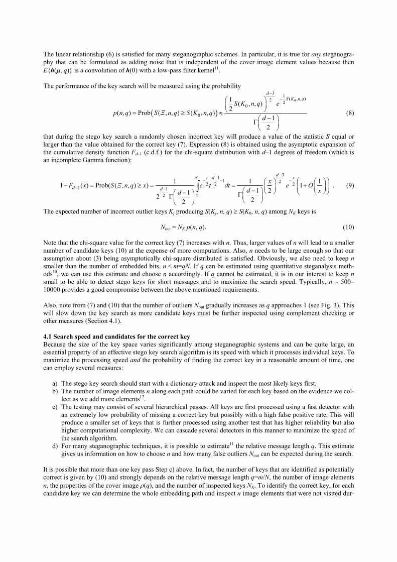
residual |r(q)| with all bins in the interval [0,+∞). The bins’ width was again chosen as σr/α with the same value of α = 0.9 and with d = 5. We have performed a number of different experiments in order to gain understanding of which factors influence the key search the most. As the first simple experiment, we searched for the correct key among 220 keys in one image embedded with ±1 embedding (see Fig. 2).

0 1 2 3 4 5 6 7 8 9 10

x 10 5

0 10 20 30 40 50 60 70 80 90

100

stat

istic

S

key number

correct key

0 10 20 30 40 50 60 70 80 90 100statistic S

correct key

Figure 2. Statistic S (3) (left) and its PDF (right) generated from 2 keys Kj

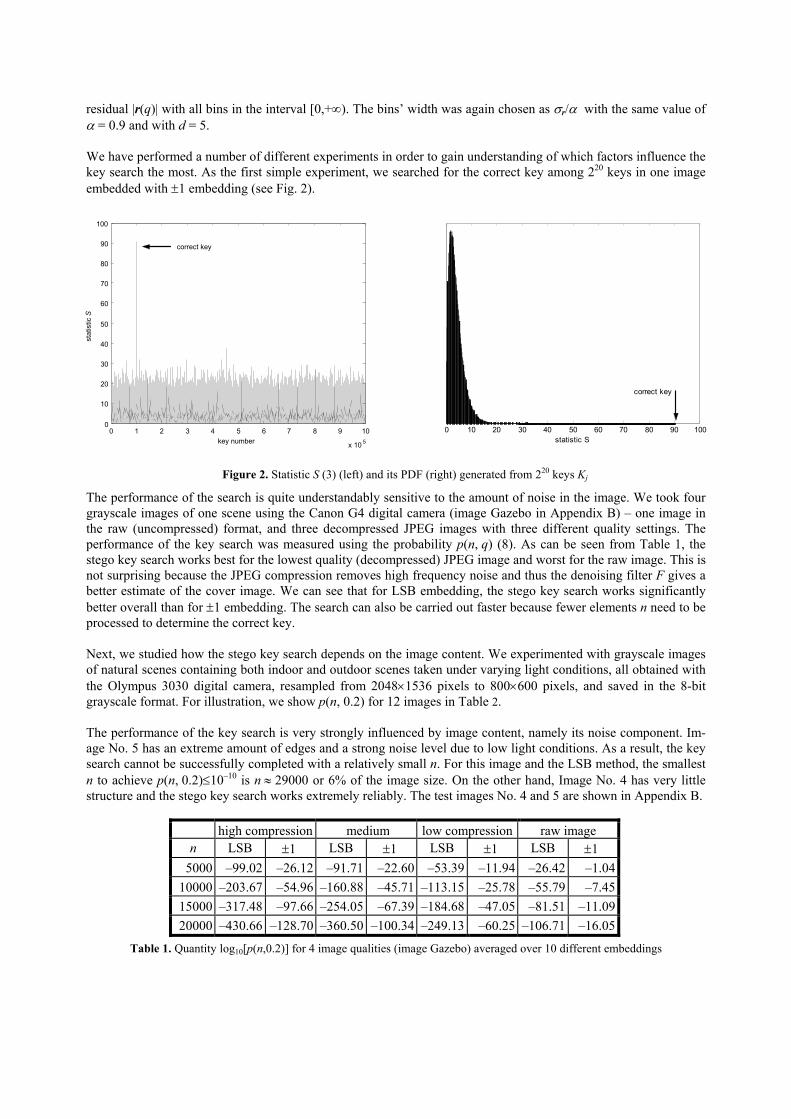
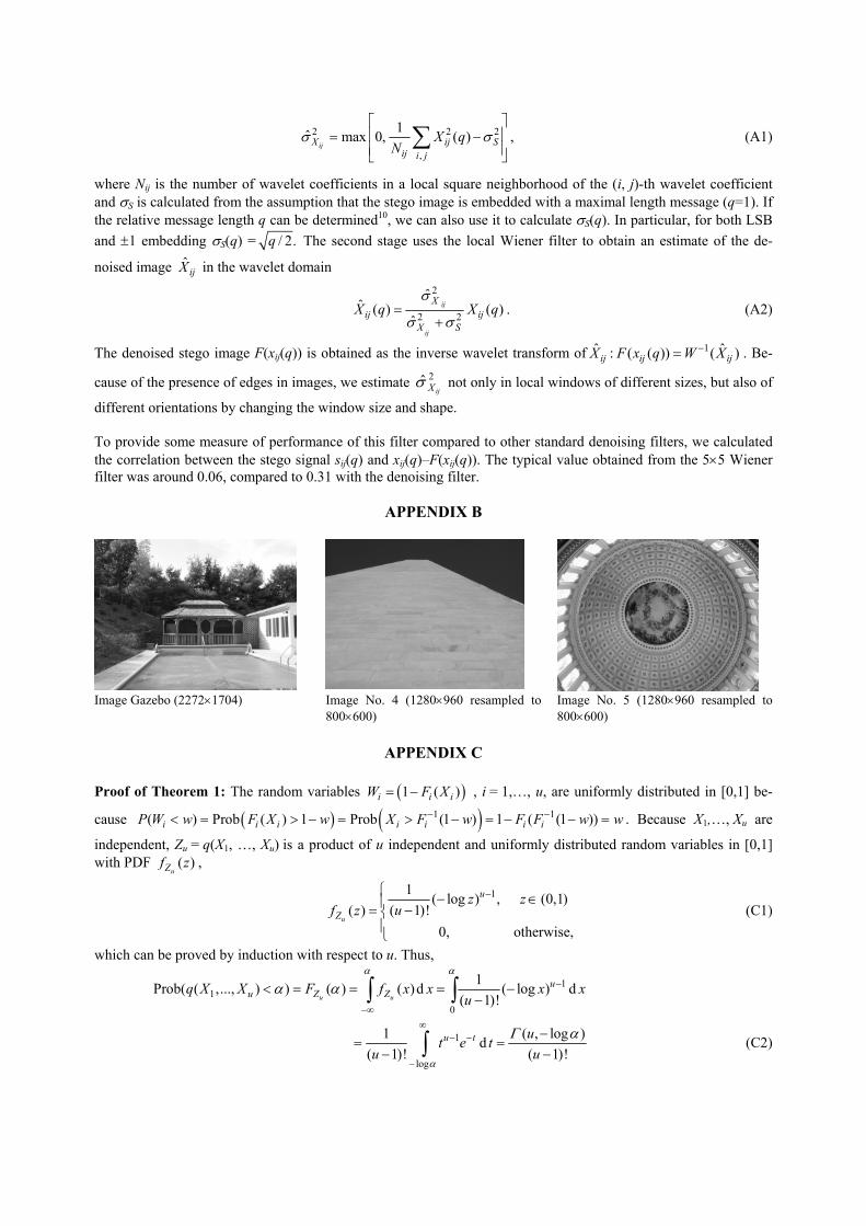
The performance of the search is quite understandably sensitive to the amount of noise in the image. We took four grayscale images of one scene using the Canon G4 digital camera (image Gazebo in Appendix B) – one image in the raw (uncompressed) format, and three decompressed JPEG images with three different quality settings. The performance of the key search was measured using the probability p(n, q) (8). As can be seen from Table 1, the stego key search works best for the lowest quality (decompressed) JPEG image and worst for the raw image. This is not surprising because the JPEG compression removes high frequency noise and thus the denoising filter F gives a better estimate of the cover image. We can see that for LSB embedding, the stego key search works significantly better overall than for ±1 embedding. Th

20

e search can also be carried out faster because fewer elements n need to be rocessed to determine the correct key.

×600 pixels, and saved in the 8-bit rayscale format. For illustration, we show p(n, 0.2) for 12 images in Table 2.

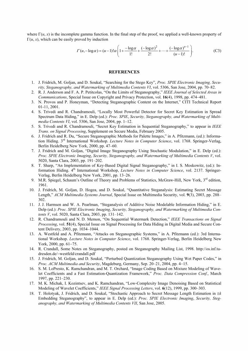
ructure and the stego key search works extremely reliably. The test images No. 4 and 5 are shown in Appendix B.

h

p Next, we studied how the stego key search depends on the image content. We experimented with grayscale images of natural scenes containing both indoor and outdoor scenes taken under varying light conditions, all obtained with the Olympus 3030 digital camera, resampled from 2048×1536 pixels to 800g The performance of the key search is very strongly influenced by image content, namely its noise component. Im-age No. 5 has an extreme amount of edges and a strong noise level due to low light conditions. As a result, the key search cannot be successfully completed with a relatively small n. For this image and the LSB method, the smallest n to achieve p(n, 0.2)≤10–10 is n ≈ 29000 or 6% of the image size. On the other hand, Image No. 4 has very little st

igh com essio me m low com raw ge n LSB ±1 LSB ±1 LSB ±1 LSB ±1

5000 –99.02 –26.12 –91.71 –22.60 –53.39 –11.94 –26.42 –1.04 10000 –203.67 –54.96 –160.88 –45.71 –113.15 –25.78 –55.79 –7.45 15000 –317.48 –97.66 –254.05 –67.39 –184.68 –47.05 –81.51 –11.09

pr n diu pression ima

20000 –430.66 –128.70 –360.50 –100.34 –249.13 –60.25 –106.71 –16.05

Table 1. Quantity log10[p(n,0.2)] for 4 image qualities (image Gazebo) averaged over 10 different embeddings

Fig. 3 shows the outlier probability p(n, q) for different relative message length q averaged over 20 different em-beddings for each q. One can clearly see how the outlier probability increases as q approaches 1 thus slowing down

e key search (as discussed in Section 4). We also see that for short messages, p(n, q) exhibits quite a large vari-ance over different mbeddings.

th e

LSB ±1 # =10000 n=20000 n=40000 =10000 20000 =40000 1 – –224.05 –19.87 –37.09 111.70 –531.51 –95.19 2 –61.39 –158.74 –317.81 –12.22 –29.64 –60.54 3 – – – –18.31 40.86 110.32 –1.13 –3.78 20.40 4 –224.54 –492.18 –1104.06 –43.86 –101.61 –243.26 5 –2.94 –5.93 –14.64 –0.11 –0.20 –0.21 6 –114.09 –254.82 –549.07 –48.47 –128.41 –279.93 7 – –165.11 –363.03 –773.72 –63.78 133.15 –318.05 8 –129.43 –256.11 –519.33 –35.62 –76.39 –153.53 9 –85.89 –202.93 –491.85 –18.14 –143.07 –57.04

10 – –31.97 –162.58 125.30 –297.02 –654.55 –74.83

Image n n n= n

11 –58.34 –125.33 –270.96 –7.56 –20.17 –51.69 12 .82 –69.20 –140.93 –266.50 –9.97 –21.05 –38

0 0.1 0.2 0.3 0.4 0.5 0.6 0.7 0.8 0.9 1q

Figure 3. Logarithm of outlier probability for different relative message length q averaged over 20 different embeddi

Table 2. Quantity log10[p(n,0.2)] av

-40 -35 -30 -25 -20 -15 -10 -5 0

log 10

[p(n

,q)]

ngs for image No. 8 with n=8000 elements. The

e

plete em-edding path must be generated. Thus, t(n) is usually the

d a Pentium IV machine HT (hyper threading) running at 2.4GHz, 512MB, 3200 DDR RAM. The ecessity to generate the whole embedding path slowed down the key search considerably, producing only 11

keys/second.

from all images may uniquely and decisively determine

raged over 10 different embeddings.

We now address the complexity of the key search. Note that the filtering as well as binning of each value ri can be done only once before the key search begins. For each candidate key Kj, we need to generate the first n elements of Path(Kj) (time needed is t(n)), then construct the histogram of their bin indices (n additions), and finally calculate the statistic (3) (3d arithmetic opera-tions). Note that t(n) is at least linear in n and could even be proportional to N, the number of all pixels, for some steganographic programs for which the combdominant term for the key search complexity. We have implemented a generic LSB embedder with a path generator that produced the whole embedding path (t(n)=O(N)) to extract the first n elements. In particular, we used the C++ Standard Template Library function std::random_shuffle, a 800×600 grayscale image,

n = 0.05N, an

boxes indicate lower quartile, median, and upper quartile values.

n

6. STEGO KEY SEARCH USING MULTIPLE IMAGES

In the case when the stego image is of low quality (noisy) or contains a complex texture or when the key space is very large, our key search algorithm may not provide enough evidence about the correct secret key (there may be too many candidate keys) even after applying the measures of Section 4.1. It is not unreasonable to assume, how-ever, that a forensic analyst will have more than one stego image embedded with the same stego key, which in-creases her chances to identify the correct key. Let us assume that the analyst has u stego images J1, …, Ju embed-ded with the same key K0, but possibly different messages. Although the measure p(n, q) (8) may not provide con-vincing evidence about the correct key for each particular image (see Table 3 that shows p(n, q) for the correct key and one incorrect key), some cumulative evidence obtained

the correct key. It is not clear, however, how such evidence should be calculated and how the performance of the

i j i j

stego key search should be measured for mu

For each image J and key K , let α (K ) =

ltiple images.

( )1 ( , , )1d jF S K n q− , where− S is defined in (3). Recalling (8), the per-

form was evaluated using

i

ance of the key sear Jich for the single image

p (n, q) = P ( )0rob ( , , ) ( , , )S n q S K n qΞ ≥

= ( ) ( )( ) ( ) ( )( )1 1 0 0Prob ( , , ) ( , , ) Probd d i iF S n q F S K n q KΞ α Ξ α− −≥ =

wj from u images, we take the product

(Kj) = α1(Kj)…αu(Kj). Obviously, the smaller α(K ) is, the larger our evidence for the key Kj. Generalizing (8) to u images and dropping the dependence on

< ,

hich is the probability that a randomly chosen key will produce a value of S larger than the one for the correct key K0 for image Ji. As a (heuristic) cumulative evidence for key Kα j

, we define n and q for brevity

p(u) = ( )0Prob ( ) ( )Kα Ξ α< (11)

as the measure of performance the stego search fo images.

for key r u

J1 J2 J3 J4 α(Kj) p(u) K : p(n, q) 1.58×10–4 1.26×10–3 2.00×10–12 3.97×10–5 1.58×10–23 4.04×10–19

0

K1: p(n, q) 7.16×10–5 8.03×10–4 6.39×10–2 2.21×10–1 8.12×10–10 1.44×10–6

Table 3. Example of collecting evidence from 4 images. Note that while the evidence in favor of each key is inconclusive, the

The expected number of incorrect keys (outliers) that produce values α(Kj) < α(K0) is

cumulative measure p(u) allows reaching an unambiguous decision when all four images are consi e.

culate p(u), we apply Theor n

dered at the same tim

out ( ) ( )KN u N p u= . To cal-em 1 below (proved i Appendix C) to the case when Fi = 1dF − , iX ( ,S , )Ξ n q= , for

image Ji, and q(X1, …, Xu) = ( )( )11u

d iF X−−∏ 1i=

= α1(Ξ)…αu(Ξ). Thus, from

10( log ( ))u iKα− −

(11) and (13) we have

ou 0( )K KN Kα ∑ . (12) t ( ) ( )N u N p u= =

1

)u

i

0 !i i=

Theorem 1. Let q(x1, x2,…, xu) = (1 ( )i iF x−∏ e a function of u real v re i=

b ariables xi, whe F are cumulative den-

sity functions of u independent variables Xi. If 1iF − exists for all Xi (i.e., ( )1 ( )i iF F x x− = for all x and i), then for 0

< α ≤ 1 2 1( , log ) log ( log ) ( log )uuΓ α α α αα α

− − − − −< = = + + + +1Prob( ( ,..., ) ) 1 ...

( 1)! 1! 2! ( 1)!uq X Xu u

− − . (13)

tego images embedded sing a key-dependent steganographic scheme. This work is thus a bridge between steganography detection and

appropriately defined statistic that quantifies statistical properties of pixels along portions of the embedding path.

7. SUMMARY AND COUNTERMEASURES

In this paper, we present a methodology for identifying the stego key from one or more sumessage extraction and is likely to be of interest to law enforcement and forensic analysts. In our approach, we focus on steganographic techniques in the spatial domain that embed one bit per image ele-ment. We assume that we have a complete knowledge of the embedding algorithm and at least one stego image. The stego key search does not rely on any recognizable patterns in the embedded bit-stream (i.e., it can be en-crypted). Instead, the stego key is determined through an exhaustive stego key search by an outlier value of an

We derive expressions for the expected number of falsely determined keys as a function of the relative embedded message length, the image content, and the number of pixels taken along each tested path. We discuss measures

at can be taken to identify the correct key from possible candidate keys determined by the search.

each steganographic embedding mechanism, the stego key search perform-nce can likely be further improved.

. If the stego key search can be searched in a reasonable time, this method could be used as a etection method.

ker guesses the correct stego key, she will have no information at ll about which pixels were used for embedding.

c easure that combines the evidence obtained from multiple images and improves the reliability of the key search.

ACKNOWLEDGEMENTS

nting the of al policies, either expressed or implied, of Air Force Research Laboratory, or the U. S. Government.

APPENDIX A

r justification of the stego message model, see Ref. 18. In the first stage, we estimate the cover image variance

th Although the search methodology is applicable to virtually all steganographic schemes, this paper focuses on two different embedding paradigms – the LSB and ±1 embedding in the spatial domain. For spatial steganography, prior to the stego key search a special non-linear high-pass filter is applied to the stego image to improve the SNR be-tween the stego signal and the cover image residual. The denoising filter has a major effect on the search perform-ance. By designing a filter matched toa The existence of fast stego key search algorithms underlines the need for strong steganographic keys. Combining a strong encryption algorithm with an insufficient stego key space may actually lead to successful attacks on the embedding schemed Besides making the stego keyspace large or slowing down the pseudo-random path generator, there is one simple countermeasure that effectively prevents stego key searches similar to the one described in this paper. If the em-bedding scheme can, in principle, use every image element with the same probability, independently of the message length, our stego key search will fail. However, padding messages to their maximal length would not be safe as this would make the stego channel more vulnerable to attacks. Instead, we recommend the selection channel2 or the matrix embedding14. For both methods, on average the groups along the correct embedding path will have the same properties as groups along an incorrect path. Moreover, the matrix embedding minimizes the number of embedding changes, which further increases the steganographic security. Lastly, steganographic schemes that use the wet paper codes15 provide an elegant and effective countermeasure because the sender does not have to share the pixel selec-tion rule with the recipient. Thus, even if the attaca In the case when the stego image is of low quality (noisy) or contains a complex texture or when the keyspace is very large, our key search algorithm may not provide enough evidence about the correct secret key (there may be too many candidate keys) even after applying the measures of Section 4.1. Clearly, having more than one stego image embedded with the same stego key increases our chances to identify the correct key. We proposed a heuristim

The work on this paper was supported by the Air Force Research Laboratory, Air Force Material Command, USAF, under research grant number F30602-02-2-0093. The U.S. Government is authorized to reproduce and distribute reprints for Governmental purposes notwithstanding any copyright notation there on. The views and conclusions contained herein are those of the authors and should not be interpreted as necessarily represe

fici

The denoising filter is based on the work first proposed in Ref. 16 and extended in Ref. 17. It is constructed in the wavelet domain while modeling the wavelet coefficients as a conditionally independent zero-mean Gaussian mix-ture process with identically distributed highly correlated variances. In this appendix, we consider the cover and stego images as two-dimensional signals indexed using two indices, i and j, where i and j are row and column indi-ces. For a message of relative length q, let xij(q), xij, and sij(q) be the values of the stego image, cover image, and the stego signal, respectively. Assuming the act of message embedding is an additive process in the spatial domain, xij(q)=xij+sij(q), we have Xij(q)=Xij+Sij(q) for the corresponding wavelet transforms Xij=W(xij), etc. In this appendix, capital letters will denote wavelet transforms of corresponding lower case variables. We model Sij(q) as a white Gaussian noise N(0,σS

2), Xij as a locally stationary i.i.d. signal with zero mean, and build the denoising filter in two stages. Fo

2 2 2

,

1ˆ max 0, ( )ijX ij S

ij i j

X qN

σ σ = −

∑ , (A1)

where N is the number of et coefficients in a local square neighborhood of the (i, j)-th wavelet coefficient and σS is calcu ed from the assumption t

ij

hat the stego image is embedded with a maximal length message (q=1). If the relative m e length can be determ σS(q). In particular, for both LSB and ±1 embedding σS(q) =

wavel

qlat

essag ined10, we can also use it to calculate ond stage uses the local Wiener filter to obtain an estimate of the de-/ 2.q The sec

noised image ˆijX in the wavelet domain

2

2

ˆ( ) ( )

ˆij

ij ij2ijXˆ

X SX q X q

σ

σ σ= . (A2)

+

The denoised stego image F(xij(q)) is obtained as the inverse wavelet transform of ˆijX : 1 ˆ( ( )) ( )ij ijF x q W X−= . Be-

To provide some measure of performance of this o other standard denoising filters, we calculated the correlation between the stego signal sij(q) and xij(q)– xij(q)). The typical value obtained from the 5×5 Wiener

cause of the presence of edges in images, we estimate 2ˆijXσ not only in local windows of different sizes, but also of

different orientations by changing the window size and shape.

filter compared tF(

filter was around 0.06, comp

ared to 0.31 with the denoising filter.

APPENDIX B

Image Gazebo (2272×1704) Image No. 4 (128 960 resampled to Image No. 5 (1280×960 resampled to 0×

800×600 800×600)

Proof of T m

)

APPENDIX C

heore 1: The random variables ( )1 ( )i iW F X= − i , i = 1,…, u, are uniformly

( ) distributed in [0,1] be-

cause ( )1 1− −( ) Prob ( ) 1 ))i i iP W w F X w w< = > − = . Because X1,…, Xu are

independent, Zu = q(X1, …, Xu) with PDF ( )

uZ

Prob (1 ) 1 ( (1i i i iw X F w F F− = > − = −

is a product of u independent and uniformly distributed random variables in [0,1] f z ,

1( log ) , (0,1)( 1)!( )

0, otherwise,u

u

Zz z

uf z−− ∈ −=

which can be proved by induction with respect to u. Thus,

1 (C1)

11( )d ( log ) d( 1)!u u

uZf x x x x

u

α α−= = −

−∫ ∫1Prob( ( ,..., ) ) ( )u Zq X X Fα α< = 0−∞

1 (∞

= 1

log

, log )d( 1)! ( 1)!

u t ut e tu u

α

Γ α− −

−

−=

− −∫ (C2)

where Γ(u, x) is the incompl known property of Γ(u, x), which can be easily

ete gamma function. In the final step of the proof, we applied a well- proved by induction

2 1u− log ( log ) ( log )( , log ) ( 1)! 11! 2! ( 1)!

u uu

α α αΓ α α − − −− = − + + + + −

. (C3)

18. essage Length Estimation in ±k Embedding Steganography”, to appear in E. Delp (ed.): Proc. SPIE Electronic Imaging, Security, Steg-anography, and Watermarking of Multimedia Contents VII, San Jose, 2005.

REFERENCES

1. J. Fridrich, M. Goljan, and D. Soukal, “Searching for the Stego Key”, Proc. SPIE Electronic Imaging, Secu-rity, Steganography, and Watermarking of Multimedia Contents VI, vol. 5306, San Jose, 2004, pp. 70–82.

2. R. J. Anderson and F. A. P. Petitcolas, “On the Limits of Steganography,” IEEE Journal of Selected Areas in Communications, Special Issue on Copyright and Privacy Protection, vol. 16(4), 1998, pp. 474–481.

3. N. Provos and P. Honeyman, “Detecting Steganographic Content on the Internet,” CITI Technical Report 01-11, 2001.

4. S. Trivedi and R. Chandramouli, “Locally Most Powerful Detector for Secret Key Estimation in Spread Spectrum Data Hiding,” in E. Delp (ed.): Proc. SPIE, Security, Steganography, and Watermarking of Multi-media Contents VI, vol. 5306, San Jose, 2004, pp. 1–12.

5. S. Trivedi and R. Chandramouli, “Secret Key Estimation in Sequential Steganography,” to appear in IEEE Trans. on Signal Processing, Supplement on Secure Media, February 2005.

6. J. Fridrich and R. Du, “Secure Steganographic Methods for Palette Images,” in A. Pfitzmann, (ed.): Informa-tion Hiding. 3rd International Workshop. Lecture Notes in Computer Science, vol. 1768. Springer-Verlag, Berlin Heidelberg New York, 2000, pp. 47–60.

7. J. Fridrich and M. Goljan, “Digital Image Steganography Using Stochastic Modulation,” in E. Delp (ed.): Proc. SPIE Electronic Imaging, Security, Steganography, and Watermarking of Multimedia Contents V, vol. 5020, Santa Clara, 2003, pp. 191–202.

8. T. Sharp, “An Implementation of Key-Based Digital Signal Steganography,” in I. S. Moskowitz, (ed.): In-formation Hiding. 4th International Workshop, Lecture Notes in Computer Science, vol. 2137. Springer-Verlag, Berlin Heidelberg New York, 2001, pp. 13–26.

9. M.R. Spiegel, Schaum’s Outline of Theory and Problems of Statistics, McGraw-Hill, New York, 3rd edition, 1961.

10. J. Fridrich, M. Goljan, D. Hogea, and D. Soukal, “Quantitative Steganalysis: Estimating Secret Message Length,” ACM Multimedia Systems Journal, Special Issue on Multimedia Security, vol. 9(3), 2003, pp. 288–302.

11. J. J. Harmsen and W. A. Pearlman, “Steganalysis of Additive Noise Modelable Information Hiding,” in E. Delp (ed.): Proc. SPIE Electronic Imaging, Security, Steganography, and Watermarking of Multimedia Con-tents V, vol. 5020, Santa Clara, 2003, pp. 131–142.

12. R. Chandramouli and N. D. Memon, “On Sequential Watermark Detection,” IEEE Transactions on Signal Processing, vol. 51(4), Special Issue on Signal Processing for Data Hiding in Digital Media and Secure Con-tent Delivery, 2003, pp. 1034–1044.

13. A. Westfeld and A. Pfitzmann, “Attacks on Steganographic Systems,” in A. Pfitzmann (ed.): 3rd Interna-tional Workshop. Lecture Notes in Computer Science, vol. 1768. Springer-Verlag, Berlin Heidelberg New York, 2000, pp. 61−75.

14. R. Crandall, Some Notes on Steganography, posted on Steganography Mailing List, 1998. http://os.inf.tu-dresden.de/~westfeld/crandall.pdf

15. J. Fridrich, M. Goljan, and D. Soukal, “Perturbed Quantization Steganography Using Wet Paper Codes,” in Proc. ACM Multimedia and Security, Magdeburg, Germany, Sep. 20–21, 2004, pp. 4−15.

16. S. M. LoPresto, K. Ramchandran, and M. T. Orchard, “Image Coding Based on Mixture Modeling of Wave-let Coefficients and a Fast Estimation-Quantization Framework,” Proc. Data Compression Conf., March 1997, pp. 221–230.

17. M. K. Michak, I. Kozintsev, and K. Ramchandran, “Low-Complexity Image Denoising Based on Statistical Modeling of Wavelet Coefficients,” IEEE Signal Processing Letters, vol. 6(12), 1999, pp. 300–303. T. Holotyak, J. Fridrich, and D. Soukal, “Stochastic Approach to Secret M