Fnl Report7842679769

ULTIMATE STRENGTH ANALYSIS OF PLATES WITH INITIAL IMPERFECTIONS

Indian Register of Shipping, Mumbai

Research & Rule Development (Structures)

Submitted by :

NIKHILESH MADDHESHIYA

INDIAN MARITIME UNIVERSITY

Internship Period from 2nd June to 26thJuly, 2014

Under the supervision of :Dr.Suhas C. Vhanmane

Senior Surveyor

Research and Rule Development Division

Indian Register of Shipping

ACKNOWLEDGEMENT

I have taken efforts in this project. However, it would not have been possible without the kind support and help of many individuals and organization. I would like to extend my sincere thanks to all of them.

I would like to express my sincere gratitude to the management of Indian Register of Shipping (IRS) for giving me an opportunity to do an internship in the organization. I am highly indebted to Dr.Suhas C. Vhanmane for his guidance and constant supervision as well as for providing necessary information regarding the project and also for his support in completing the project. I would also like to thank Dr. A Samanta, Head of the Structures department who had reviewed my work and given valuable suggestions to improve the quality of my project.

Table of Contents1. Introduction To Finite Element Analysis 1

1.1 WHAT IS FINITE ELEMENT ANALYSIS 2

1.2 How Does Finite Element Analysis Work 3

1.3 Types Of Engineering Analysis 3

1.4 Results of Finite Element Analysis 3

2. Introduction To ANSYS 4

2.1 ANSYS Environment 5

2.2 ANSYS Interface 6

2.3 Convergence Testing 6

2.4 Saving or Restoring job 6

2.4 ANSYS files 6

2.4 Printing Results 6

3. Nonlinear Analysis 4

3.1 Introduction to nonlinear analysis 6

3.2 Reasons for nonlinear analysis 6

3.3 Consequences of nonlinear analysis 6

3.4 Types of nonlinearity 6

3.5 Basic concept of nonlinear analysis 6

1. Introduction To Finite Element Analysis

1.1 What Is Finite Element Analysis (FEA)?

FEA consists of a computer model of a material or design that is stressed and

analyzed for specific results. It is used in new product design, and existing

product refinement. A company is able to verify a proposed design will be able

to perform to the client's specifications prior to manufacturing or construction.

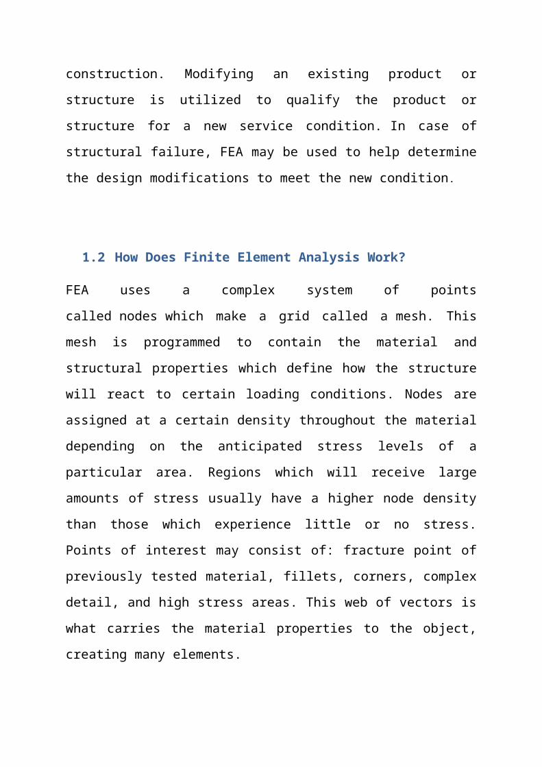
Modifying an existing product or structure is utilized to qualify the product or

structure for a new service condition. In case of structural failure, FEA may be

used to help determine the design modifications to meet the new condition.

1.2 How Does Finite Element Analysis Work?

FEA uses a complex system of points called nodes which make a grid called

a mesh. This mesh is programmed to contain the material and structural

properties which define how the structure will react to certain loading

conditions. Nodes are assigned at a certain density throughout the material

depending on the anticipated stress levels of a particular area. Regions which

will receive large amounts of stress usually have a higher node density than

those which experience little or no stress. Points of interest may consist of:

fracture point of previously tested material, fillets, corners, complex detail, and

high stress areas. This web of vectors is what carries the material properties to

the object, creating many elements. 

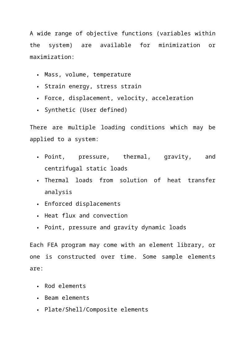
A wide range of objective functions (variables within the system) are available

for minimization or maximization:

Mass, volume, temperature

Strain energy, stress strain

Force, displacement, velocity, acceleration

Synthetic (User defined)

There are multiple loading conditions which may be applied to a system:

Point, pressure, thermal, gravity, and centrifugal static loads

Thermal loads from solution of heat transfer analysis

Enforced displacements

Heat flux and convection

Point, pressure and gravity dynamic loads

Each FEA program may come with an element library, or one is constructed

over time. Some sample elements are:

Rod elements

Beam elements

Plate/Shell/Composite elements

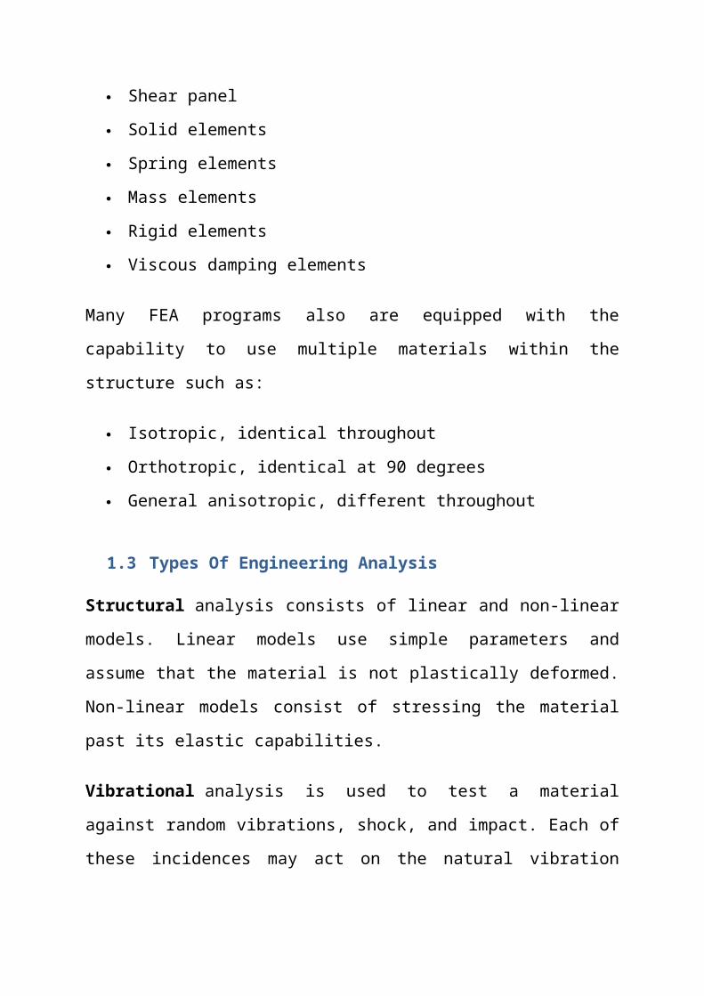
Shear panel

Solid elements

Spring elements

Mass elements

Rigid elements

Viscous damping elements

Many FEA programs also are equipped with the capability to use multiple

materials within the structure such as:

Isotropic, identical throughout

Orthotropic, identical at 90 degrees

General anisotropic, different throughout

1.3 Types Of Engineering Analysis

Structural analysis consists of linear and non-linear models. Linear models use

simple parameters and assume that the material is not plastically deformed.

Non-linear models consist of stressing the material past its elastic capabilities.

Vibrational analysis is used to test a material against random vibrations, shock,

and impact. Each of these incidences may act on the natural vibration frequency

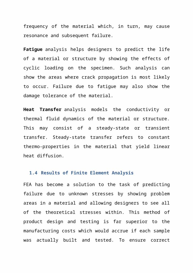
of the material which, in turn, may cause resonance and subsequent failure.

Fatigue analysis helps designers to predict the life of a material or structure by

showing the effects of cyclic loading on the specimen. Such analysis can show

the areas where crack propagation is most likely to occur. Failure due to fatigue

may also show the damage tolerance of the material.

Heat Transfer analysis models the conductivity or thermal fluid dynamics of

the material or structure. This may consist of a steady-state or transient transfer.

Steady-state transfer refers to constant thermo-properties in the material that

yield linear heat diffusion. 

1.4 Results of Finite Element Analysis

FEA has become a solution to the task of predicting failure due to unknown

stresses by showing problem areas in a material and allowing designers to see

all of the theoretical stresses within. This method of product design and testing

is far superior to the manufacturing costs which would accrue if each sample

was actually built and tested. To ensure correct results in a Finite Element

Analysis, the element type should be carefully chosen and the meshing should

be fine enough to capture all the minute details.

2. Introduction to ANSYS

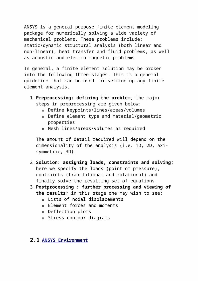
ANSYS is a general purpose finite element modeling package for numerically solving a wide variety of mechanical problems. These problems include: static/dynamic structural analysis (both linear and non-linear), heat transfer and fluid problems, as well as acoustic and electro-magnetic problems.

In general, a finite element solution may be broken into the following three stages. This is a general guideline that can be used for setting up any finite element analysis.

1. Preprocessing: defining the problem; the major steps in preprocessing are given below:

o Define keypoints/lines/areas/volumes

o Define element type and material/geometric propertieso Mesh lines/areas/volumes as required

The amount of detail required will depend on the dimensionality of the analysis (i.e. 1D, 2D, axi-symmetric, 3D).

2. Solution: assigning loads, constraints and solving; here we specify the loads (point or pressure), contraints (translational and rotational) and finally solve the resulting set of equations.

3. Postprocessing : further processing and viewing of the results; in this stage one may wish to see:

o Lists of nodal displacementso Element forces and momentso Deflection plotso Stress contour diagrams

2.1 ANSYS Environment

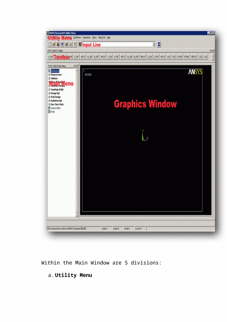
The ANSYS Environment for ANSYS 14.0 contains 2 windows : the Main Window and an Output Window. Note that this is somewhat different from the previous version of ANSYS which made use of 6 different windows.

1. Main Window

Within the Main Window are 5 divisions:

a. Utility Menu

The Utility Menu contains functions that are available throughout the ANSYS session, such as file controls, selections, graphic controls and parameters.

b. Input window

The Input Line shows program prompt messages and allows you to type in commands directly.

c. Toolbar

The Toolbar contains push buttons that execute commonly used ANSYS commands. More push buttons can be added if desired.

d. Main Menu

The Main Menu contains the primary ANSYS functions, organized by preprocessor, solution, general postprocessor, design optimizer. It is from this menu that the vast majority of modelling commands are issued. This is where you will note the greatest change between previous versions of ANSYS and version 7.0. However, while the versions appear different, the menu structure has not changed.

e. Graphics Window

The Graphic Window is where graphics are shown and graphical picking can be made. It is here where you will graphically view the model in its various stages of construction and the ensuing results from the analysis.

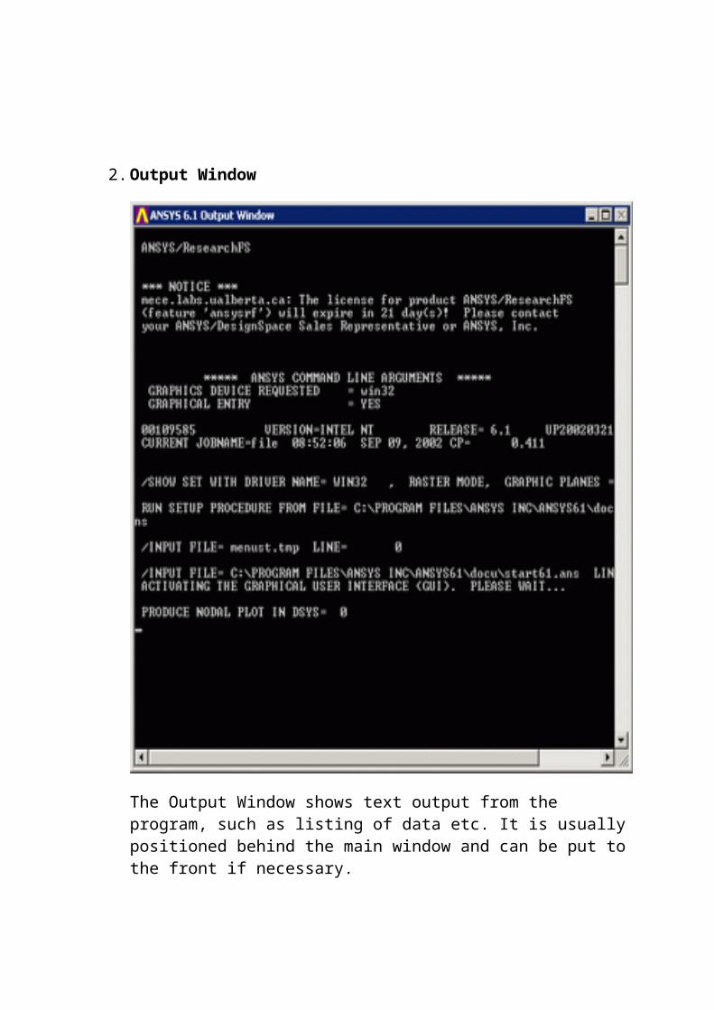
2. Output Window

The Output Window shows text output from the program, such as listing of data etc. It is usually positioned behind the main window and can be put to the front if necessary.

2.2 ANSYS Interface

Graphical Interface vs. Command File Coding

There are two methods to use ANSYS. The first is by means of the graphical user interface or GUI. This method follows the conventions of popular Windows and X-Windows based programs.

The second is by means of command files. The command file approach has a steeper learning curve for many, but it has the advantage that an entire analysis can be described in a small text file, typically in less than 50 lines of commands. This approach enables easy model modifications and minimal file space requirements.

For information and details on the full ANSYS command language, consult:

Help > Table of Contents > Commands Manual.

2.3 Convergence Testing

IntroductionA fundamental premise of using the finite element procedure is that the body is sub-divided up into small discrete regions known as finite elements. These elements defined by nodes and interpolation functions. Governing equations are written for each element and these elements are assembled into a global matrix. Loads and constraints are applied and the solution is then determined.

The ProblemThe question that always arises is: How small do I need to make the elements before I can trust the solution?

What to do about it...In general there are no real firm answers on this. It will be necessary to conduct convergence tests! By this we mean that you begin with a mesh discretization and then observe and record the solution. Now repeat the problem with a finer mesh (i.e. more elements) and then compare the

results with the previous test. If the results are nearly similar, then the first mesh is probably good enough for that particular geometry, loading and constraints. If the results differ by a large amount however, it will be necessary to try a finer mesh yet.

The ConsequencesFiner meshes come with a cost however : more calculation time and large memory requirements (both disk and RAM)! It is desired to find the minimum number of elements that give you a converged solution.

General ModelsIn general however, it is necessary to conduct convergence tests on your finite element model to confirm that a fine enough element discretization has been used. In a solid mechanics problem, this would be done by creating several models with different mesh sizes and comparing the resulting deflections and stresses, for example. In general, the stresses will converge more slowly than the displacement, so it is not sufficient to examine the displacement convergence.

2.4 Saving/Restoring Jobs

Saving Your JobIt is good practice to save your model at various points during its creation. Very often you will get to a point in the modeling where things have gone well and you like to save it at the point. In that way, if you make some mistakes later on, you will at least be able to come back to this point.

To save your model, select  Utility Menu Bar -> File -> Save

As Jobname.db. Your model will be saved in a file called jobname.db, where jobname is the name that you specified in the Launcher when you first started ANSYS.

It is a good idea to save your job at different times throughout the building and analysis of the model to backup your work in case of a system crash or other unforeseen problems.

Recalling or Resuming a Previously Saved Job

Frequently you want to start up ANSYS and recall and continue a previous job. There are two methods to do this:

1. Using the Launcher...o In the ANSYS Launcher, select Interactive... and

specify the previously defined jobname.o Then when you get ANSYS started, select Utility Menu -

> File -> Resume Jobname.db.o This will restore as much of your database (geometry, loads,

solution, etc) that you previously saved.2. Or, start ANSYS and select Utitily Menu -> File ->

Resume from... and select your job from the list that appears.

2.5 ANSYS Files

IntroductionA large number of files are created when you run ANSYS. If you started ANSYS without specifying a jobname, the name of all the files created will be FILE.* where the * represents various extensions described below. If

you specified a jobname, say Frame, then the created files will all have the

file prefix, Frame again with various extensions:

frame.db

Database file (binary). This file stores the geometry, boundary conditions and any solutions.

frame.dbb

Backup of the database file (binary).

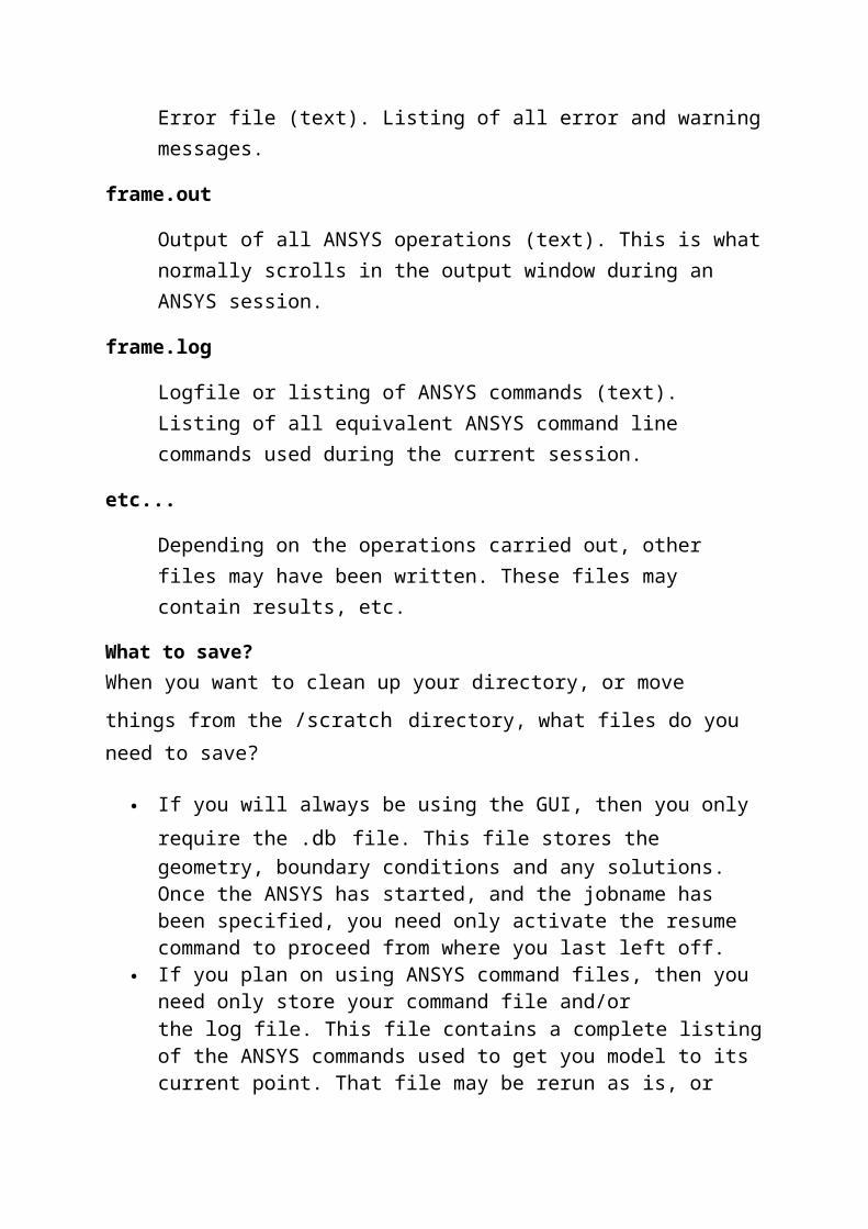
frame.err

Error file (text). Listing of all error and warning messages.

frame.out

Output of all ANSYS operations (text). This is what normally scrolls in the output window during an ANSYS session.

frame.log

Logfile or listing of ANSYS commands (text). Listing of all equivalent ANSYS command line commands used during the current session.

etc...

Depending on the operations carried out, other files may have been written. These files may contain results, etc.

What to save?When you want to clean up your directory, or move things from

the /scratch directory, what files do you need to save?

If you will always be using the GUI, then you only require

the .db file. This file stores the geometry, boundary conditions and any solutions. Once the ANSYS has started, and the jobname has been specified, you need only activate the resume command to proceed from where you last left off.

If you plan on using ANSYS command files, then you need only store your command file and/or the log file. This file contains a complete listing of the ANSYS commands used to get you model to its current point. That file may be rerun as is, or edited and rerun as desired (Command File Creation and Execution).

If you plan to use the command mode of operation, starting with an existing  log file, rename it first so that it does not get over-written or added to, from another ANSYS run.

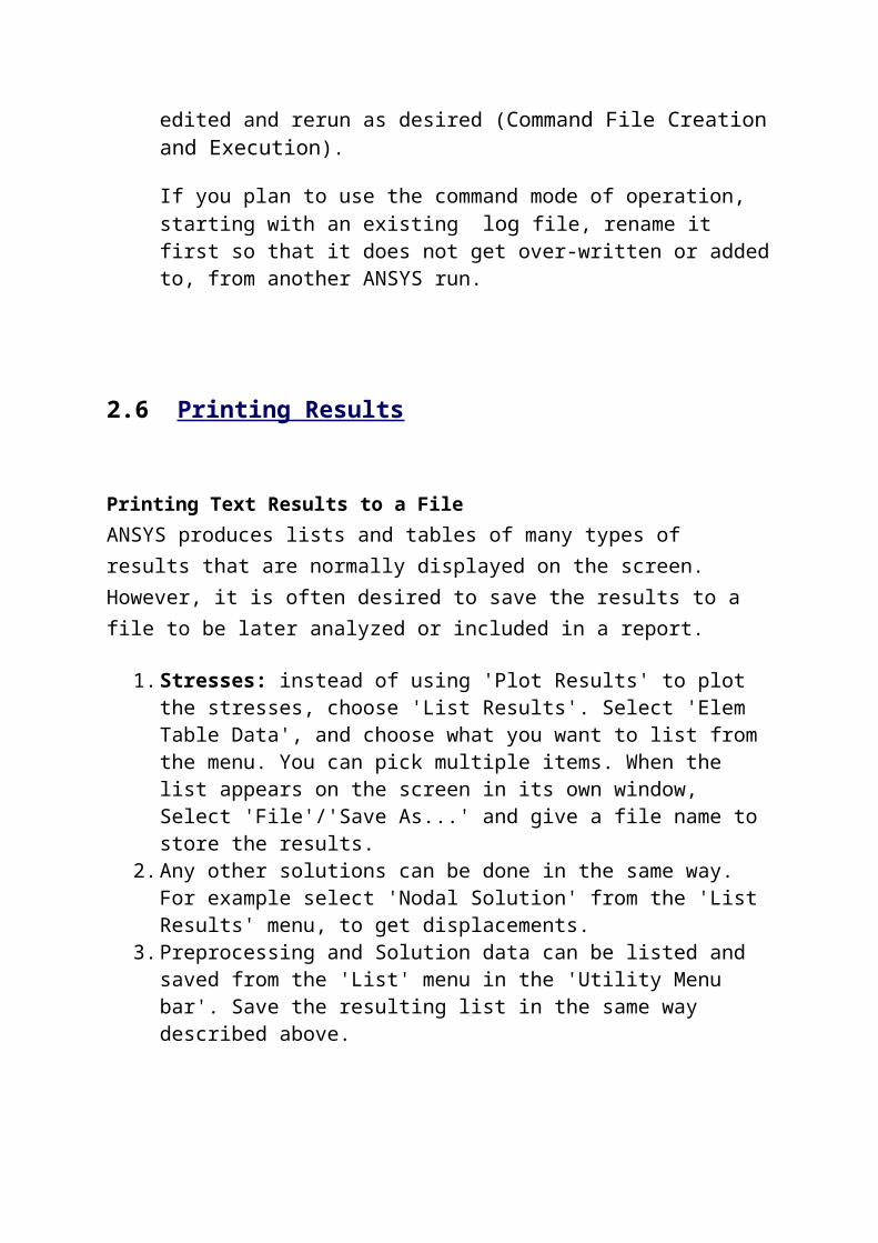
2.6 Printing Results

Printing Text Results to a FileANSYS produces lists and tables of many types of results that are normally displayed on the screen. However, it is often desired to save the results to a file to be later analyzed or included in a report.

1. Stresses: instead of using 'Plot Results' to plot the stresses, choose 'List Results'. Select 'Elem Table Data', and choose what you want to list from the menu. You can pick multiple items. When the list appears on the screen in its own window, Select 'File'/'Save As...' and give a file name to store the results.

2. Any other solutions can be done in the same way. For example select 'Nodal Solution' from the 'List Results' menu, to get displacements.

3. Preprocessing and Solution data can be listed and saved from the 'List' menu in the 'Utility Menu bar'. Save the resulting list in the same way described above.

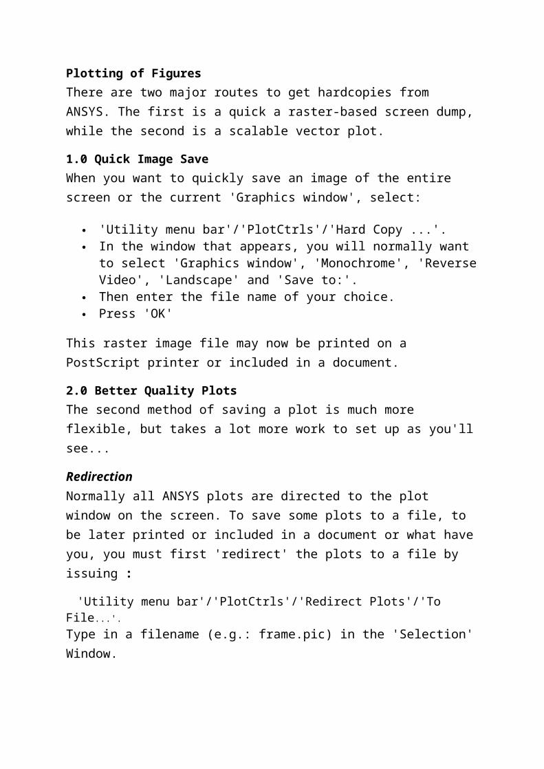
Plotting of FiguresThere are two major routes to get hardcopies from ANSYS. The first is a quick a raster-based screen dump, while the second is a scalable vector plot.

1.0 Quick Image SaveWhen you want to quickly save an image of the entire screen or the current 'Graphics window', select:

'Utility menu bar'/'PlotCtrls'/'Hard Copy ...'. In the window that appears, you will normally want to select 'Graphics

window', 'Monochrome', 'Reverse Video', 'Landscape' and 'Save to:'. Then enter the file name of your choice. Press 'OK'

This raster image file may now be printed on a PostScript printer or included in a document.

2.0 Better Quality PlotsThe second method of saving a plot is much more flexible, but takes a lot more work to set up as you'll see...

RedirectionNormally all ANSYS plots are directed to the plot window on the screen. To save some plots to a file, to be later printed or included in a document or what have you, you must first 'redirect' the plots to a file by issuing :

'Utility menu bar'/'PlotCtrls'/'Redirect Plots'/'To File...'.Type in a filename (e.g.: frame.pic) in the 'Selection' Window.

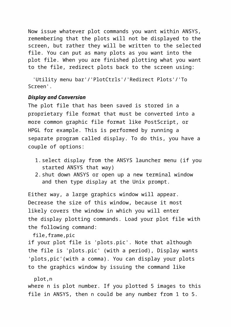
Now issue whatever plot commands you want within ANSYS, remembering that the plots will not be displayed to the screen, but rather they will be written to the selected file. You can put as many plots as you want into the plot file. When you are finished plotting what you want to the file, redirect plots back to the screen using:

'Utility menu bar'/'PlotCtrls'/'Redirect Plots'/'To Screen'.

Display and ConversionThe plot file that has been saved is stored in a proprietary file format that must be converted into a more common graphic file format like PostScript, or HPGL for example. This is performed by running a separate program called display. To do this, you have a couple of options:

1. select display from the ANSYS launcher menu (if you started ANSYS that way)

2. shut down ANSYS or open up a new terminal window and then type display at the Unix prompt.

Either way, a large graphics window will appear. Decrease the size of this window, because it most likely covers the window in which you will enter the display plotting commands. Load your plot file with the following

command: file,frame,picif your plot file is 'plots.pic'. Note that although the file is 'plots.pic' (with a period), Display wants 'plots,pic'(with a comma). You can display your plots to the graphics window by issuing the command like

plot,nwhere n is plot number. If you plotted 5 images to this file in ANSYS, then n could be any number from 1 to 5.

Now that the plots have been read in, they may be saved to printer files of various formats:

1. Colour PostScript: To save the images to a colour postscript file, enter the following commands in display:

2. pscr,color,23. /show,pscr4. plot,n

where n is the plot number, as above. You can plot as many images as you want to postscript files in this manner. For subsequent plots, you only require the plot,n command as the other options have

now been set. Each image is plotted to a postscript file such as pscrxx.grph, where xx is a number, starting at 00.

Note: when you import a postscript file into a word processor, the postscript image will appear as blank box. The printer information is still present, but it can only be viewed when it's printed out to a postscript printer.

5. Black & White PostScript: The above mentioned colour postscript files can get very large in size and may not even print out on the postscript printer in the lab because it takes so long to transfer the files to the printer and process them. A way around this is to print them out in a black and white postscript format instead of colour; besides the colour specifications don't do any good for the black and white lab printer anyways. To do this, you set the postscript color option to '3', i.e. and then issue the other commands as before

6. pscr,color,37. /show,pscr8. plot,n

Note: when you import a postscript file into a word processor, the postscript image will appear as blank box. The printer information is still present, but it can only be viewed when it's printed out to a postscript printer.

9. HPGL: The third commonly used printer format is HPGL, which stands for Hewlett Packard Graphics Language. This is a compact vector format that has the advantage that when you import a file of this type into a word processor, you can actually see the image in the word processor! To use the HPGL format, issue the following commands:

10. /show,hpgl11. plot,n

Final Steps

It is wise to rename these plot files as soon as you leave display,

for display will overwrite the files the next time it is run. You may

want to rename the postscript files with an '.eps' extension to indicate

that they are encapsulated postscript images. In a similar way, the HPGL printer files could be given an '.hpgl' extension. This renaming is done at the Unix commmand line (the 'mv' command).

A list of all available display commands and their options may be obtained by typing:

help

When complete, exit display by entering

finish

3. NONLINEAR ANALYSIS

3.1 INTRODUCTION TO NONLINEAR ANALYSIS Some important engineering phenomena can only be assessed on the basis of a nonlinear analysis:

• Collapse or buckling of structures due to sudden overloads

• Progressive damage behavior due to long lasting severe loads

• For certain structures (e.g. cables), nonlinear phenomena need be included in the analysis even for service load calculations.

The need for nonlinear analysis has increased in recent years due to the need for

- use of optimized structures

- use of new materials

- addressing safety-related issues of structures more rigorously

The corresponding benefits can be most important.

Problems to be addressed by a nonlinear finite element analysis are found in almost all branches of engineering, most notably in,

Nuclear Engineering

Earthquake Engineering

Automobile Industries

Defense Industries

Aeronautical Engineering

Mining Industries

Offshore Engineering and so on.

A nonlinear analysis is needed if the loading on a structure causes significant changes in stiffness. Typical reasons for stiffness to change significantly are:

– Strains beyond the elastic limit (plasticity)

– Large deflections, such as with a loaded fishing rod

– Contact between two bodies

Linear v/s Nonlinear Response

• Numerical simulation of the response where both the LHS and RHS depends

upon the primary unknown.

• Linear versus Nonlinear FEA:

Linear FEA:

[K]{D}={R}

Nonlinear FEA:

[K(D)]{D}={R(D)}

• Field of Nonlinear FEA:

Continuum mechanics FE discretization (FEM) Numerical solution algorithms Software considerations (engineering)

Equilibrium path

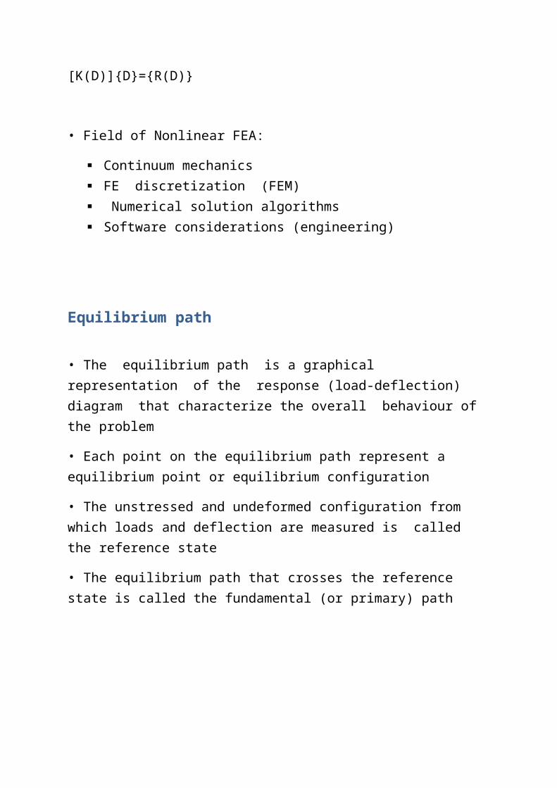
• The equilibrium path is a graphical representation of the response (load-deflection) diagram that characterize the overall behaviour of the problem

• Each point on the equilibrium path represent a equilibrium point or equilibrium configuration

• The unstressed and undeformed configuration from which loads and deflection are measured is called the reference state

• The equilibrium path that crosses the reference state is called the fundamental (or primary) path

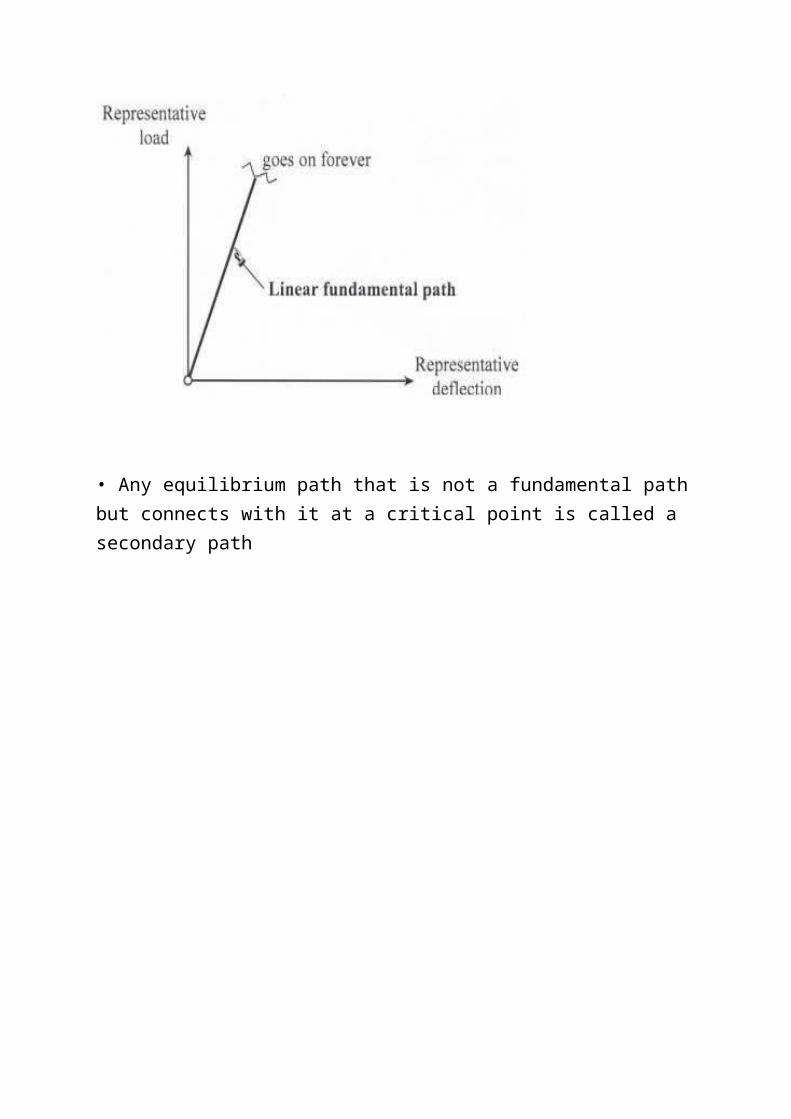
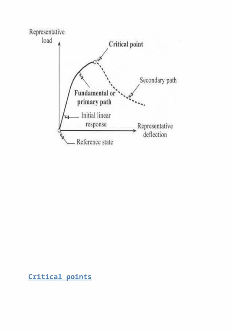
• Any equilibrium path that is not a fundamental path but connects with it at a critical point is called a secondary path

Critical points

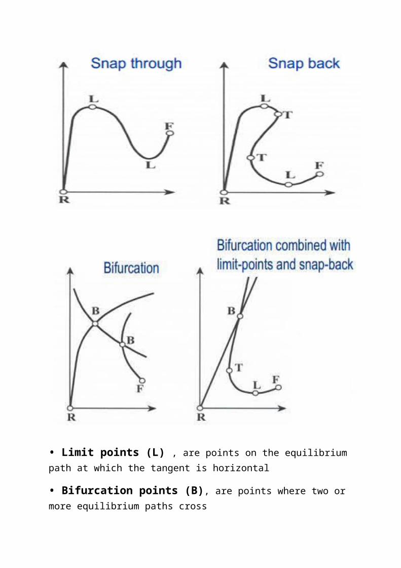
• Limit points (L) , are points on the equilibrium path at which the tangent is horizontal

• Bifurcation points (B), are points where two or more equilibrium paths cross

• Turning points (T), are points where the tangent is vertical

• Failure points (F), are points where the path suddenly stops because of physical failure.

Advantages of linear response

• A linear structure can sustain any load whatsoever and undergo any displacement magnitude

• There are no critical (limit, bifurcation, turning or failure) points

• Solutions for various load cases may be superimposed

• Removing all loads returns the structure to the reference state

• Simple direct solution of the structural stiffness relationship without need for costly load incrementation and iterative schemes

3.2 Reasons for Nonlinear FEA

• Strength analysis – how much load can the structure support before global failure occurs

• Stability analysis – finding critical points (limit points and bifurcation points) closest to operational range

• Service configuration analysis – finding the ‘operational’ equilibrium configuration of certain slender structures when the fabrication and service configurations are quite different (e.g. cable and inflatable structures)

• Reserve strength analysis – finding the load carrying capacity beyond critical points to assess safety under abnormal conditions

• Progressive failure analysis – a combined strength and stability analysis in which progressive detoriation (e.g. cracking) is considered

• Establish the causes of a structural failure

• Safety and serviceability assessment of existing infrastructure whose integrity may be in doubt due to:

– Visible damage (cracking, etc)

–Special loadings not envisaged at the design state

– Health–monitoring

– Concern over corrosion or general aging

• A shift towards high performance materials and more efficient utilization of structural components

• Direct use of NFEA in design for both ultimate load and serviceability limit states

• Simulation of materials processing and manufacturing (e.g. metal forming, extrusion and casting processes)

• In research:

– To establish simple ‘code-based’ methods of analysis and design

– To understand basic structural behaviour

– To test the validity of proposed ‘material models’

• Computer hardware becomes cheaper and faster and FE software becomes more robust and user-friendly

• It will simply become easier for an engineer to apply direct analysis rather than code-based checking.

3.3 Consequences of Nonlinear FEA

• For the analyst familiar with the use of LFEA, there are a number of consequences of nonlinear behavior that have to be recognized before embarking on a NFEA:

The principle of superposition cannot be applied Results of several ‘load cases’ cannot be scaled, factored and combined

as is done with LFEA Only one load case can be handled at a time The loading history (i.e. sequence of application of loads) may be

important The structural response can be markedly non-proportional to the

applied loading, even for simple loading states Careful thought needs to be given to what is an appropriate measure of

the behavior The initial state of stress(e.g. residual stresses from welding,

temperature, or prestressing of reinforcement and cables) may be extremely important for the overall response

3.4 TYPES OF NONLINEARITY

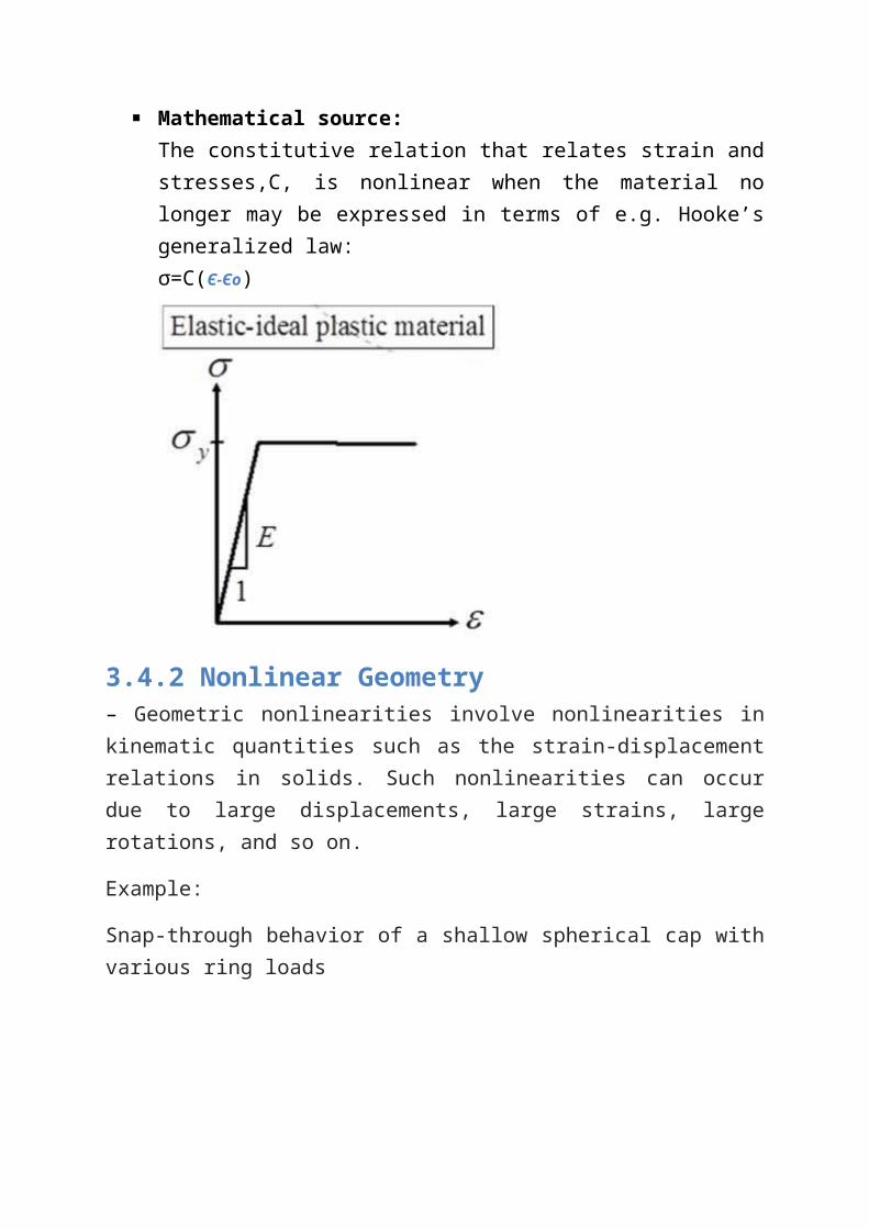
3.4.1 Nonlinear Material Physical source:

Material behavior depends on current deformation state and possibly past history of the deformation.

The constitutive relation may depend on other variables (prestress, temperature, time, moisture, electromagnetic fields, etc)

Applications:–Nonlinear elasticity–Plasticity–Viscoelasticity–Creep, or inelastic rate effects

Mathematical source:The constitutive relation that relates strain and stresses,C, is nonlinear when the material no longer may be expressed in terms of e.g. Hooke’s generalized law:σ=C( - oЄ Є )

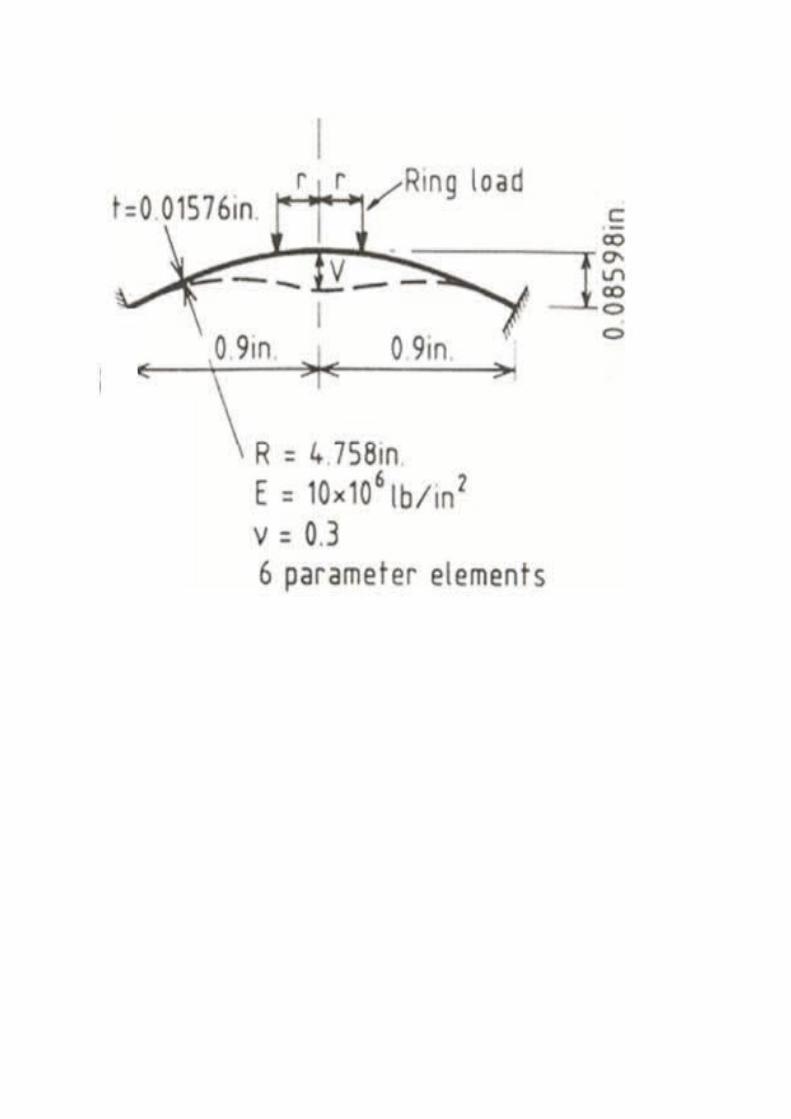
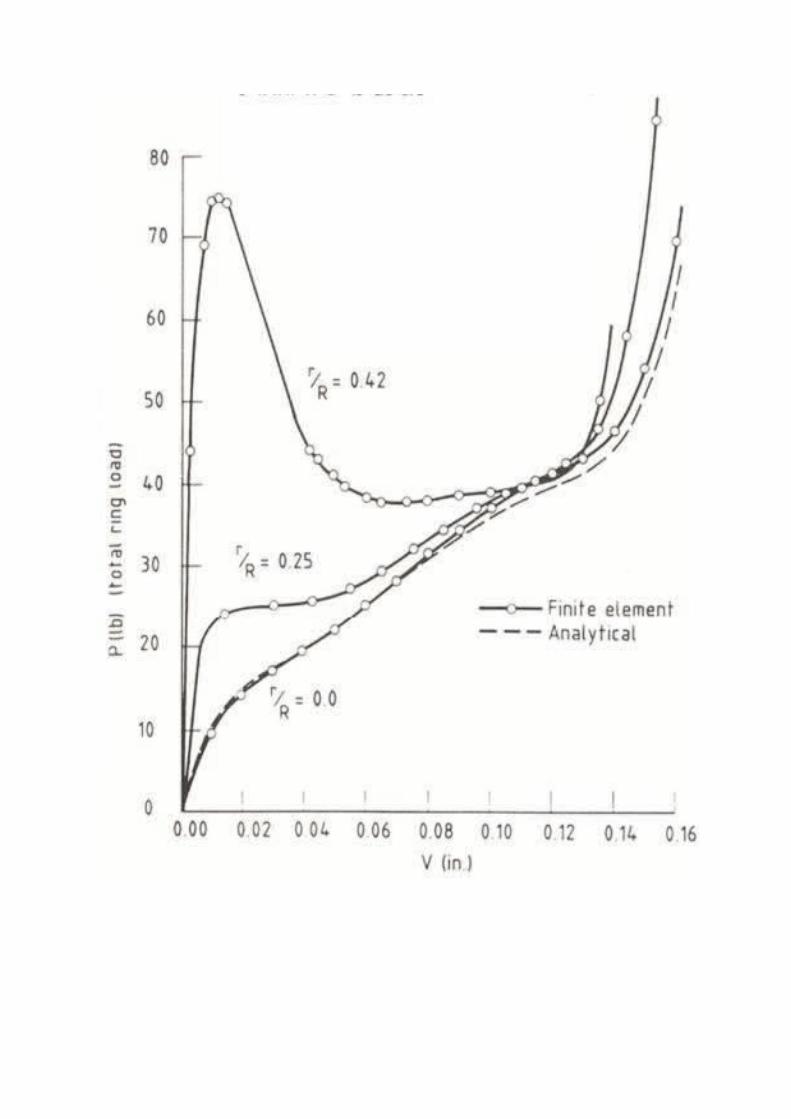
3.4.2 Nonlinear Geometry– Geometric nonlinearities involve nonlinearities in kinematic quantities such as the strain-displacement relations in solids. Such nonlinearities can occur due to large displacements, large strains, large rotations, and so on.

Example:

Snap-through behavior of a shallow spherical cap with various ring loads

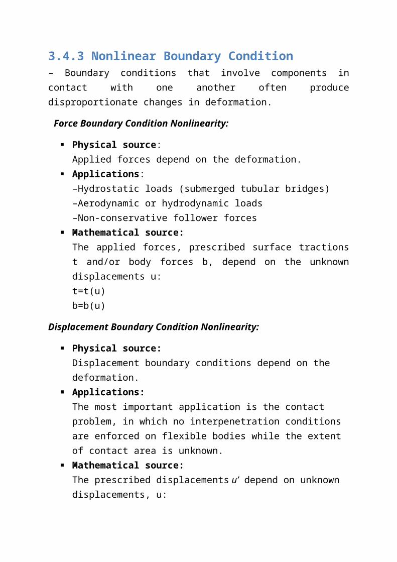
3.4.3 Nonlinear Boundary Condition– Boundary conditions that involve components in contact with one another often produce disproportionate changes in deformation.

Force Boundary Condition Nonlinearity:

Physical source: Applied forces depend on the deformation.

Applications:–Hydrostatic loads (submerged tubular bridges)–Aerodynamic or hydrodynamic loads–Non-conservative follower forces

Mathematical source:The applied forces, prescribed surface tractions t and/or body forces b, depend on the unknown displacements u:t=t(u)b=b(u)

Displacement Boundary Condition Nonlinearity:

Physical source: Displacement boundary conditions depend on the deformation.

Applications:The most important application is the contact problem, in which no interpenetration conditions are enforced on flexible bodies while the extent of contact area is unknown.

Mathematical source:The prescribed displacements u’ depend on unknown displacements, u: u’=u’(u)

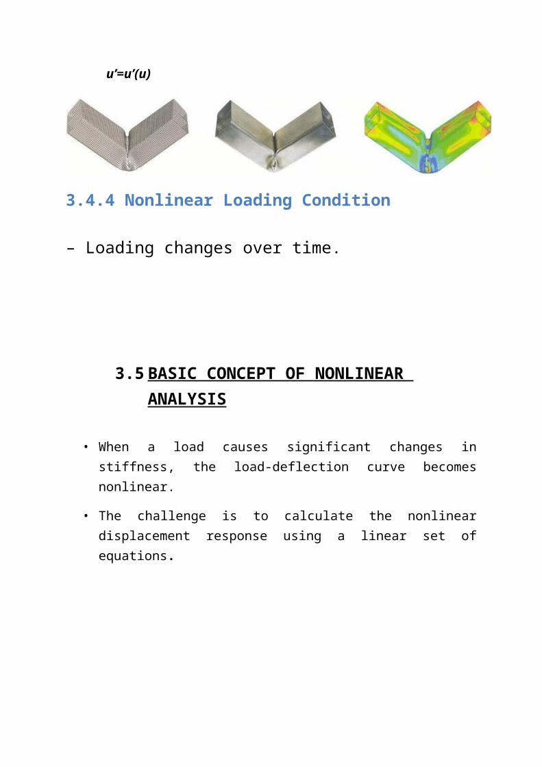
3.4.4 Nonlinear Loading Condition

– Loading changes over time.

3.5 BASIC CONCEPT OF NONLINEAR ANALYSIS

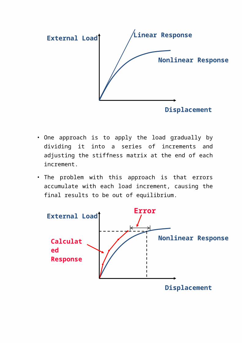
• When a load causes significant changes in stiffness, the load-deflection curve becomes nonlinear.

• The challenge is to calculate the nonlinear displacement response using a linear set of equations.

• One approach is to apply the load gradually by dividing it into a series of increments and adjusting the stiffness matrix at the end of each increment.

• The problem with this approach is that errors accumulate with each load increment, causing the final results to be out of equilibrium.

Nonlinear Response

Linear Response

Displacement

External Load

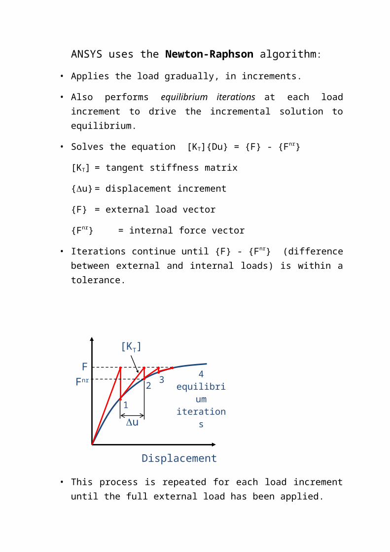
ANSYS uses the Newton-Raphson algorithm:

• Applies the load gradually, in increments.

• Also performs equilibrium iterations at each load increment to drive the incremental solution to equilibrium.

• Solves the equation [KT]{Du} = {F} - {Fnr}

[KT] = tangent stiffness matrix

{Du} = displacement increment

{F} = external load vector

{Fnr} = internal force vector

• Iterations continue until {F} - {Fnr} (difference between external and internal loads) is within a tolerance.

Nonlinear Response

Displacement

External LoadError

Calculated Response

• This process is repeated for each load increment until the full external load has been applied.

3.5.1 Weaknesses of Newton’s method

• The standard (true) Newton’s method, although effective in most cases, is not necessarily the most economical solution method and does not always provide rapid and reliable convergence.

• Weaknesses of the method:

Computational expense: ─Tangent stiffness has to be computed and assembled at each iteration within each load step─If a direct solver is employed Kt also needs to be factored at each iteration within each load step

Increment size:─If the time stepping algorithm used is not robust (self-adaptive), a certain degree of trial and error may be required to determine the appropriate load increments

Divergence:─If the equilibrium path include critical points negative load increments must be prescribed to go beyond limit points─If the load increments are too large such that the solution falls outside ‘‘the ball of convergence’’ analysis may fail to converge

Displacement

F

[KT]

1

23

4 equilibrium iterationsFnr

Du

3.5.2Modified Newton methods• Modified Newton methods differ from the standard method in that the tangent stiffness Kt is only

updated occasionally.

• Initial stiffness method:

Tangent stiffness Kt updated only once The method may result in a slow rate of convergence

• Modified Newton’s method:

Tangent stiffness Kt updated occasionally (but not for every iteration) More rapid convergence than the initial stiffness method (but not

quadratic)

• Quasi (secant) Newton methods:

The inverse of the tangent stiffness obtained by a secant approximation rather than recomputing and factorizing Kt at every iteration

Thus a nonlinear solution typically involves the following:

– One or more load steps to apply the external loads and boundary conditions. (This is true of linear analyses too.)

– Multiple substeps to apply the load gradually. Each substep represents one load increment. (A linear analysis needs just one substep per load step.)

– Equilibrium iterations to obtain equilibrium (or convergence) at each substep. (Does not apply to linear analyses.)

Time and Time Step

• Each load step and substep is associated with a value of time.

• Time in most nonlinear static analyses is simply used as a counter and does not mean actual, chronological time.

"Time"

External Load

Substeps

LS 1

Load Step (LS) 2

– By default, time = 1.0 at the end of load step 1, 2.0 at the end of load step 2, and so on.

– For rate-independent analyses, you can set it to any desired value for convenience. For example, by setting time equal to the load magnitude, you can easily plot the load-deflection curve.

• The "time increment" between each substep is the time step Dt.

• Time step Dt determines the load increment DF over a substep. The higher the value of Dt, the larger the DF, so Dt has a direct effect on the accuracy of the solution.

• ANSYS has an automatic time stepping algorithm that predicts and controls the time step size for all substeps in a load step.

3.5.3 Choosing step length

• The optimal choice of the incremental step depends on:

The shape of the equilibrium path:Large increments may be used were the path is almost linear and smaller ones where the curve is highly nonlinear

The objective of the analysis:If it is necessary to trace the entire equilibrium path accurately, small increments are needed, while if only the failure load is of interest, largersteps can be used until the load is close to the limit value

The solution algorithm employed: The initial stiffness method require smaller increments than the modified Newton’s method that again require smaller increments than the standard Newton’s method

• It is desirable that the solution algorithm includes a solution monitoring device that on basis of:

Certain user prescribed input, and Degree of nonlinearity of the equilibrium path is able to adjust the size

of the load increment

"Time"

External Load

1.0 2.0

Dt

DF

3.5.4 Load incrementation• For monotonic loading, the load increment can be based on number of iterations:

∆ λ n=∆ λ n−1 √ N d

N n−1

(∆ λ min≤∆ λ n≤ ¿)

Where N d is a ‘desired number of iterations’selected by the analyst,N n−1 is the number of iterations required for convergence at increment ‘n-1’, while ∆ λ max and ∆ λ min are upper and lower limit of the increment prescribed by the analyst.

• However, the initial load increment still have to be selected by the analyst

3.5.4.1 Automatic load incrementation

• Even though you may find more sophisticated incremental load control methods, they can only work effectively if nonlinearity spreads gradually.

• Such methods cannot predict a sudden change in the stiffness.

• Solution methods based on prescribed load {Rnext }= {Rext (λ n)} or prescribed displacements {Dn }={D( λn)} are not able to trace the equilibrium path beyond limit and turning points, respectively.

3.5 Convergence criteria

• A convergence criteria measures how well the obtained solution satisfies equilibrium.

• In NFEA of the convergence criteria are usually based on some norm of the:

Displacements (total or incremental) Residuals Energy (product of residual and displacement)

• Although displacement based criteria seem to be the most natural choice they are not advisable in general as they can be misleadingly satisfied by a slow convergence rate.

• Residual based criteria are far more reliable as they check that equilibrium has been achieved within a specified tolerance in the current increment.

• Alternatively energy based criteria that use both displacements and residuals may be applied However, energy criteria should not be used together with LS.

• In general NFEA it is recommended that a combination of the three criteria is applied.

• The convergence criteria and tolerances must be carefully chosen so as to provide accurate yet economical solutions.

If the convergence criterion is too loose inaccurate results are obtained. If the convergence criterion is too tight too much effort spent in

obtaining unnecessary accuracy.