Flexible Parametric Survival Analysis Using Stata: Beyond ... · book on survival analysis in Stata (Cleves et al. 2010): This is a book about survival analysis for the professional

Flexible Parametric Survival Analysis

Using Stata: Beyond the Cox Model

PATRICK ROYSTONMRC Clinical Trials Unit, United Kingdom

PAUL C. LAMBERTDepartment of Health Sciences, University of Leicester, United Kingdom and

Medical Epidemiology and Biostatistics, Karolinska Institute, Stockholm, Sweden

®

A Stata Press PublicationStataCorp LPCollege Station, Texas

® Copyright c© 2011 by StataCorp LP

All rights reserved. First edition 2011

Published by Stata Press, 4905 Lakeway Drive, College Station, Texas 77845

Typeset in LATEX2ε

Printed in the United States of America

10 9 8 7 6 5 4 3 2 1

ISBN-10: 1-59718-079-3

ISBN-13: 978-1-59718-079-5

Library of Congress Control Number: 2011921921

No part of this book may be reproduced, stored in a retrieval system, or transcribed, in any

form or by any means—electronic, mechanical, photocopy, recording, or otherwise—without

the prior written permission of StataCorp LP.

Stata, , Stata Press, Mata, , and NetCourse are registered trademarks of

StataCorp LP.

Stata and Stata Press are registered trademarks with the World Intellectual Property Organi-

zation of the United Nations.

LATEX2ε is a trademark of the American Mathematical Society.

Contents

List of tables xiii

List of figures xv

Preface xxv

1 Introduction 1

1.1 Goals . . . . . . . . . . . . . . . . . . . . . . . . . . . . . . . . . . . . 1

1.2 A brief review of the Cox proportional hazards model . . . . . . . . 2

1.3 Beyond the Cox model . . . . . . . . . . . . . . . . . . . . . . . . . . 2

1.3.1 Estimating the baseline hazard . . . . . . . . . . . . . . . . 2

1.3.2 The baseline hazard contains useful information . . . . . . . 5

1.3.3 Advantages of smooth survival functions . . . . . . . . . . . 8

1.3.4 Some requirements of a practical survival analysis . . . . . . 9

1.3.5 When the proportional-hazards assumption is breached . . . 10

1.4 Why parametric models? . . . . . . . . . . . . . . . . . . . . . . . . . 13

1.4.1 Smooth baseline hazard and survival functions . . . . . . . . 13

1.4.2 Time-dependent HRs . . . . . . . . . . . . . . . . . . . . . . 13

1.4.3 Modeling on different scales . . . . . . . . . . . . . . . . . . 13

1.4.4 Relative survival . . . . . . . . . . . . . . . . . . . . . . . . 13

1.4.5 Prediction out of sample . . . . . . . . . . . . . . . . . . . . 14

1.4.6 Multiple time scales . . . . . . . . . . . . . . . . . . . . . . . 14

1.5 Why not standard parametric models? . . . . . . . . . . . . . . . . . 14

1.6 A brief introduction to stpm2 . . . . . . . . . . . . . . . . . . . . . . 16

1.6.1 Estimation (model fitting) . . . . . . . . . . . . . . . . . . . 16

1.6.2 Postestimation facilities (prediction) . . . . . . . . . . . . . 17

1.7 Basic relationships in survival analysis . . . . . . . . . . . . . . . . . 17

vi Contents

1.8 Comparing models . . . . . . . . . . . . . . . . . . . . . . . . . . . . 18

1.9 The delta method . . . . . . . . . . . . . . . . . . . . . . . . . . . . . 19

1.10 Ado-file resources . . . . . . . . . . . . . . . . . . . . . . . . . . . . . 20

1.11 How our book is organized . . . . . . . . . . . . . . . . . . . . . . . . 21

2 Using stset and stsplit 23

2.1 What is the stset command? . . . . . . . . . . . . . . . . . . . . . . . 23

2.2 Some key concepts . . . . . . . . . . . . . . . . . . . . . . . . . . . . 23

2.3 Syntax of the stset command . . . . . . . . . . . . . . . . . . . . . . 24

2.4 Variables created by the stset command . . . . . . . . . . . . . . . . 25

2.5 Examples of using stset . . . . . . . . . . . . . . . . . . . . . . . . . 25

2.5.1 Standard survival data . . . . . . . . . . . . . . . . . . . . . 26

2.5.2 Using the scale( ) option . . . . . . . . . . . . . . . . . . . . 27

2.5.3 Date of diagnosis and date of exit . . . . . . . . . . . . . . . 27

2.5.4 Date of diagnosis and date of exit with the scale( ) option . 28

2.5.5 Restricting the follow-up time . . . . . . . . . . . . . . . . . 29

2.5.6 Left-truncation . . . . . . . . . . . . . . . . . . . . . . . . . 31

2.5.7 Age as the time scale . . . . . . . . . . . . . . . . . . . . . . 32

2.6 The stsplit command . . . . . . . . . . . . . . . . . . . . . . . . . . . 33

2.6.1 Time-dependent effects . . . . . . . . . . . . . . . . . . . . . 33

2.6.2 Time-varying covariates . . . . . . . . . . . . . . . . . . . . 34

2.7 Conclusion . . . . . . . . . . . . . . . . . . . . . . . . . . . . . . . . . 35

3 Graphical introduction to the principal datasets 37

3.1 Introduction . . . . . . . . . . . . . . . . . . . . . . . . . . . . . . . . 37

3.2 Rotterdam breast cancer data . . . . . . . . . . . . . . . . . . . . . . 37

3.3 England and Wales breast cancer data . . . . . . . . . . . . . . . . . 39

3.4 Orchiectomy data . . . . . . . . . . . . . . . . . . . . . . . . . . . . . 42

3.5 Conclusion . . . . . . . . . . . . . . . . . . . . . . . . . . . . . . . . . 45

4 Poisson models 47

4.1 Introduction . . . . . . . . . . . . . . . . . . . . . . . . . . . . . . . . 47

4.2 Modeling rates with the Poisson distribution . . . . . . . . . . . . . . 48

Contents vii

4.3 Splitting the time scale . . . . . . . . . . . . . . . . . . . . . . . . . . 50

4.3.1 The piecewise exponential model . . . . . . . . . . . . . . . 53

4.3.2 Time as just another covariate . . . . . . . . . . . . . . . . . 57

4.4 Collapsing the data to speed up computation . . . . . . . . . . . . . 57

4.5 Splitting at unique failure times . . . . . . . . . . . . . . . . . . . . . 59

4.5.1 Technical note: Why the Cox and Poisson approaches areequivalent∗ . . . . . . . . . . . . . . . . . . . . . . . . . . . . 61

4.6 Comparing a different number of intervals . . . . . . . . . . . . . . . 62

4.7 Fine splitting of the time scale . . . . . . . . . . . . . . . . . . . . . 66

4.8 Splines: Motivation and definition . . . . . . . . . . . . . . . . . . . 67

4.8.1 Calculating splines∗ . . . . . . . . . . . . . . . . . . . . . . . 69

4.8.2 Restricted cubic splines . . . . . . . . . . . . . . . . . . . . . 70

4.8.3 Splines: Application to the Rotterdam data . . . . . . . . . 71

4.8.4 Varying the number of knots . . . . . . . . . . . . . . . . . . 74

4.8.5 Varying the location of the knots . . . . . . . . . . . . . . . 78

4.8.6 Estimating the survival function∗ . . . . . . . . . . . . . . . 79

4.9 FPs: Motivation and definition . . . . . . . . . . . . . . . . . . . . . 81

4.9.1 Application to Rotterdam data . . . . . . . . . . . . . . . . 83

4.9.2 Higher order FP models . . . . . . . . . . . . . . . . . . . . 87

4.9.3 FP function selection procedure . . . . . . . . . . . . . . . . 89

4.10 Discussion . . . . . . . . . . . . . . . . . . . . . . . . . . . . . . . . . 90

5 Royston–Parmar models 91

5.1 Motivation and introduction . . . . . . . . . . . . . . . . . . . . . . . 92

5.1.1 The exponential distribution . . . . . . . . . . . . . . . . . . 92

5.1.2 The Weibull distribution . . . . . . . . . . . . . . . . . . . . 95

5.1.3 Generalizing the Weibull . . . . . . . . . . . . . . . . . . . . 96

5.1.4 Estimating the hazard function . . . . . . . . . . . . . . . . 100

5.2 Proportional hazards models . . . . . . . . . . . . . . . . . . . . . . 101

5.2.1 Generalizing the Weibull . . . . . . . . . . . . . . . . . . . . 101

5.2.2 Example . . . . . . . . . . . . . . . . . . . . . . . . . . . . . 103

viii Contents

5.2.3 Comparing parameters of PH(1) and Weibull models . . . . 104

5.3 Selecting a spline function . . . . . . . . . . . . . . . . . . . . . . . . 108

5.3.1 Knot positions . . . . . . . . . . . . . . . . . . . . . . . . . . 108

Example . . . . . . . . . . . . . . . . . . . . . . . . . . . . . 109

5.3.2 How many knots? . . . . . . . . . . . . . . . . . . . . . . . . 110

5.4 PO models . . . . . . . . . . . . . . . . . . . . . . . . . . . . . . . . 111

5.4.1 Introduction . . . . . . . . . . . . . . . . . . . . . . . . . . . 111

5.4.2 The loglogistic model . . . . . . . . . . . . . . . . . . . . . . 112

5.4.3 Generalizing the loglogistic model . . . . . . . . . . . . . . . 113

5.4.4 Comparing parameters of PO(1) and loglogistic models . . . 113

Example . . . . . . . . . . . . . . . . . . . . . . . . . . . . . 114

5.5 Probit models . . . . . . . . . . . . . . . . . . . . . . . . . . . . . . . 114

5.5.1 Motivation . . . . . . . . . . . . . . . . . . . . . . . . . . . . 114

5.5.2 Generalizing the probit model . . . . . . . . . . . . . . . . . 115

5.5.3 Comparing parameters of probit(1) and lognormal models . 116

5.5.4 Comments on probit and POs models . . . . . . . . . . . . . 117

5.6 Royston–Parmar (RP) models . . . . . . . . . . . . . . . . . . . . . . 118

5.6.1 Models with θ not equal to 0 or 1 . . . . . . . . . . . . . . . 119

5.6.2 Example . . . . . . . . . . . . . . . . . . . . . . . . . . . . . 119

5.6.3 Likelihood function and parameter estimation∗ . . . . . . . 120

5.6.4 Comparing regression coefficients . . . . . . . . . . . . . . . 121

5.6.5 Model selection . . . . . . . . . . . . . . . . . . . . . . . . . 121

5.6.6 Sensitivity to number of knots . . . . . . . . . . . . . . . . . 122

5.6.7 Sensitivity to location of knots . . . . . . . . . . . . . . . . 123

5.7 Concluding remarks . . . . . . . . . . . . . . . . . . . . . . . . . . . 124

6 Prognostic models 125

6.1 Introduction . . . . . . . . . . . . . . . . . . . . . . . . . . . . . . . . 125

6.2 Developing and reporting a prognostic model . . . . . . . . . . . . . 126

6.3 What does the baseline hazard function mean? . . . . . . . . . . . . 127

6.3.1 Example . . . . . . . . . . . . . . . . . . . . . . . . . . . . . 128

Contents ix

6.4 Model selection . . . . . . . . . . . . . . . . . . . . . . . . . . . . . . 129

6.4.1 Choice of scale and baseline complexity . . . . . . . . . . . . 130

Example . . . . . . . . . . . . . . . . . . . . . . . . . . . . . 130

6.4.2 Selection of variables and functional forms . . . . . . . . . . 131

Example . . . . . . . . . . . . . . . . . . . . . . . . . . . . . 132

6.5 Quantitative outputs from the model . . . . . . . . . . . . . . . . . . 134

6.5.1 Survival probabilities for individuals . . . . . . . . . . . . . 134

6.5.2 Survival probabilities across the risk spectrum . . . . . . . . 137

6.5.3 Survival probabilities at given covariate values . . . . . . . . 138

6.5.4 Survival probabilities in groups . . . . . . . . . . . . . . . . 140

6.5.5 Plotting adjusted survival curves . . . . . . . . . . . . . . . 142

6.5.6 Plotting differences between survival curves . . . . . . . . . 143

6.5.7 Centiles of the survival distribution . . . . . . . . . . . . . . 145

6.6 Goodness of fit . . . . . . . . . . . . . . . . . . . . . . . . . . . . . . 147

6.6.1 Example . . . . . . . . . . . . . . . . . . . . . . . . . . . . . 148

6.7 Discrimination and explained variation . . . . . . . . . . . . . . . . . 149

6.7.1 Example . . . . . . . . . . . . . . . . . . . . . . . . . . . . . 151

6.7.2 Harrell’s C index of concordance . . . . . . . . . . . . . . . 152

6.8 Out-of-sample prediction: Concept and applications . . . . . . . . . 153

6.8.1 Extrapolation of survival functions: Basic technique . . . . 153

6.8.2 Extrapolation of survival functions: Further investigations . 155

6.8.3 Validation of prognostic models: Basics . . . . . . . . . . . . 157

6.8.4 Validation of prognostic models: Further comments . . . . . 160

6.9 Visualization of survival times . . . . . . . . . . . . . . . . . . . . . . 161

6.9.1 Example . . . . . . . . . . . . . . . . . . . . . . . . . . . . . 161

6.10 Discussion . . . . . . . . . . . . . . . . . . . . . . . . . . . . . . . . . 164

7 Time-dependent effects 167

7.1 Introduction . . . . . . . . . . . . . . . . . . . . . . . . . . . . . . . . 167

7.2 Definitions . . . . . . . . . . . . . . . . . . . . . . . . . . . . . . . . . 168

7.3 What do we mean by a TD effect? . . . . . . . . . . . . . . . . . . . 169

x Contents

7.4 Proportional on which scale? . . . . . . . . . . . . . . . . . . . . . . 176

7.5 Poisson models with TD effects . . . . . . . . . . . . . . . . . . . . . 179

7.5.1 Piecewise models . . . . . . . . . . . . . . . . . . . . . . . . 180

7.5.2 Using restricted cubic splines . . . . . . . . . . . . . . . . . 184

7.6 RP models with TD effects . . . . . . . . . . . . . . . . . . . . . . . 190

7.6.1 Piecewise HRs . . . . . . . . . . . . . . . . . . . . . . . . . . 190

7.6.2 Continuous TD effects . . . . . . . . . . . . . . . . . . . . . 193

7.6.3 More than one TD effect . . . . . . . . . . . . . . . . . . . . 201

7.6.4 Stratification is the same as including TD effects . . . . . . 203

7.7 TD effects for continuous variables . . . . . . . . . . . . . . . . . . . 205

7.8 Attained age as the time scale . . . . . . . . . . . . . . . . . . . . . . 211

7.8.1 The orchiectomy data . . . . . . . . . . . . . . . . . . . . . 211

7.8.2 Proportional hazards model . . . . . . . . . . . . . . . . . . 212

7.8.3 TD model . . . . . . . . . . . . . . . . . . . . . . . . . . . . 214

7.9 Multiple time scales . . . . . . . . . . . . . . . . . . . . . . . . . . . 218

7.10 Prognostic models with TD effects . . . . . . . . . . . . . . . . . . . 219

7.10.1 Example . . . . . . . . . . . . . . . . . . . . . . . . . . . . . 220

7.11 Discussion . . . . . . . . . . . . . . . . . . . . . . . . . . . . . . . . . 224

8 Relative survival 227

8.1 Introduction . . . . . . . . . . . . . . . . . . . . . . . . . . . . . . . . 227

8.2 What is relative survival? . . . . . . . . . . . . . . . . . . . . . . . . 227

8.3 Excess mortality and relative survival . . . . . . . . . . . . . . . . . 228

8.3.1 Excess mortality . . . . . . . . . . . . . . . . . . . . . . . . 228

8.3.2 Relative survival is a ratio . . . . . . . . . . . . . . . . . . . 230

8.4 Motivating example . . . . . . . . . . . . . . . . . . . . . . . . . . . . 231

8.5 Life-table estimation of relative survival . . . . . . . . . . . . . . . . 233

8.5.1 Using strs . . . . . . . . . . . . . . . . . . . . . . . . . . . . 234

8.6 Poisson models for relative survival . . . . . . . . . . . . . . . . . . . 235

8.6.1 Piecewise models . . . . . . . . . . . . . . . . . . . . . . . . 235

8.6.2 Restricted cubic splines . . . . . . . . . . . . . . . . . . . . . 241

Contents xi

8.7 RP models for relative survival . . . . . . . . . . . . . . . . . . . . . 246

8.7.1 Likelihood for relative survival models . . . . . . . . . . . . 247

8.7.2 Proportional cumulative excess hazards . . . . . . . . . . . . 247

8.7.3 RP models on other scales . . . . . . . . . . . . . . . . . . . 248

8.7.4 Application to England and Wales breast cancer data . . . . 248

8.7.5 Relative survival models on other scales . . . . . . . . . . . 250

8.7.6 Time-dependent effects . . . . . . . . . . . . . . . . . . . . . 253

8.8 Some comments on model selection . . . . . . . . . . . . . . . . . . . 259

8.9 Age as a continuous variable . . . . . . . . . . . . . . . . . . . . . . . 267

8.10 Concluding remarks . . . . . . . . . . . . . . . . . . . . . . . . . . . 272

9 Further topics 273

9.1 Introduction . . . . . . . . . . . . . . . . . . . . . . . . . . . . . . . . 273

9.2 Number needed to treat . . . . . . . . . . . . . . . . . . . . . . . . . 273

9.2.1 Example . . . . . . . . . . . . . . . . . . . . . . . . . . . . . 274

9.3 Average and adjusted survival curves . . . . . . . . . . . . . . . . . . 275

9.3.1 Renal data . . . . . . . . . . . . . . . . . . . . . . . . . . . . 277

9.4 Modeling distributions with RP models . . . . . . . . . . . . . . . . 283

9.4.1 Example 1: Rotterdam breast cancer data . . . . . . . . . . 283

9.4.2 Example 2: CD4 lymphocyte data . . . . . . . . . . . . . . 285

9.4.3 Example 3: Prostate cancer data . . . . . . . . . . . . . . . 294

9.5 Multiple events . . . . . . . . . . . . . . . . . . . . . . . . . . . . . . 296

9.5.1 Introduction . . . . . . . . . . . . . . . . . . . . . . . . . . . 296

9.5.2 The AG model . . . . . . . . . . . . . . . . . . . . . . . . . 297

9.5.3 The WLW model . . . . . . . . . . . . . . . . . . . . . . . . 298

9.5.4 The PWP model . . . . . . . . . . . . . . . . . . . . . . . . 298

9.5.5 Multiple events in RP models . . . . . . . . . . . . . . . . . 298

9.5.6 Summary . . . . . . . . . . . . . . . . . . . . . . . . . . . . 304

9.6 Bayesian RP models . . . . . . . . . . . . . . . . . . . . . . . . . . . 304

9.6.1 Introduction . . . . . . . . . . . . . . . . . . . . . . . . . . . 304

9.6.2 The “zeros trick” in WinBUGS . . . . . . . . . . . . . . . . 305

xii Contents

9.6.3 Fitting a RP model . . . . . . . . . . . . . . . . . . . . . . . 305

9.6.4 Summary . . . . . . . . . . . . . . . . . . . . . . . . . . . . 310

9.7 Competing risks . . . . . . . . . . . . . . . . . . . . . . . . . . . . . . 310

9.7.1 Summary . . . . . . . . . . . . . . . . . . . . . . . . . . . . 316

9.8 Period analysis . . . . . . . . . . . . . . . . . . . . . . . . . . . . . . 317

9.8.1 Introduction . . . . . . . . . . . . . . . . . . . . . . . . . . . 317

9.8.2 What is period analysis? . . . . . . . . . . . . . . . . . . . . 317


9.9 Crude probability of death from relative survival models . . . . . . . 322

9.9.1 Introduction . . . . . . . . . . . . . . . . . . . . . . . . . . . 322


9.9.3 Conclusion . . . . . . . . . . . . . . . . . . . . . . . . . . . . 329

9.10 Final remarks . . . . . . . . . . . . . . . . . . . . . . . . . . . . . . . 329

References 331

Author index 341

Subject index 345

Preface

We would first like to quote from the preface of a well-known and respected Stata Pressbook on survival analysis in Stata (Cleves et al. 2010):

This is a book about survival analysis for the professional data analyst,whether a health scientist, an economist, a political scientist, or any of awide range of scientists who have found that survival analysis is applicableto their problems. This is a book for researchers who want to understandwhat they are doing and to understand the underpinnings and assumptionsof the tools they use; in other words, this is a book for all researchers.

In a way, the aims of our book are similar to those of Cleves et al. (2010). We extendtheir book in particular directions: flexible, parametric, going beyond the standardmodels, particularly the Cox model. We include, for example, detailed treatments oftime-dependent effects and relative survival. Our starting point is a basic understandingof survival analysis and how it is done in Stata. We would be surprised, for example, ifa reader had not created and plotted Kaplan–Meier curves and fitted a Cox model inStata. Our aim is that researchers can build on our examples to apply the methodologyto their own investigations of survival data. To that end, we have provided the basictools (ado-files) but also, in the examples, we present Stata code to do many of theanalyses and produce many of the graphs. Indeed, presentation of the results of flexibleparametric modeling is often best achieved by well-chosen graphs, and we regard thatas an important message of our book.

Royston–Parmar models are a key tool in our approach; they are currently availableonly in Stata. (See section 1.10 for more information.) We would like to see theirimplementation in other software, such as R or SAS. However, we are very unlikely toimplement this ourselves! If anyone has attempted such an implementation (or plans todo so) and would value our input, we would encourage them to contact us.

This book uses Stata version 12 throughout, but is fully compatible with Stata 11.1or later, with only minor cosmetic differences across versions.

Finally, we would like to thank the folk who have contributed to our understandingof survival analysis and those who have undertaken the seemingly thankless task ofcommenting on our draft text. We are particularly grateful to

Therese Andersson, Karolinska InstituteCarol Coupland, University of Nottingham

xxvi Preface

Paul Dickman, Karolinska InstituteSandra Eloranta, Karolinska InstituteBobby Gutierrez, StataCorpHans van Houwelingen, University of LeidenBernard Rachet, London School of Hygiene and Tropical MedicineBill Rising, StataCorpMark Rutherford, University of LeicesterWilli Sauerbrei, University of Freiburg Medical CenterMichael Schemper, University of Vienna

London and Leicester Patrick RoystonApril 2011 Paul C. Lambert

1 Introduction

1.1 Goals

Most books on survival analysis devote a substantial section of their material to the Coxproportional hazards (PH) model (Cox 1972). The Cox model has played a vital rolein applied survival analysis during the last three decades. The model and its softwareimplementations have popularized survival analysis and made it accessible to researchersin varied disciplines who are not necessarily statisticians. It has been so successful thatit is probably used in most practical analyses of the effects of covariates on survival.

Some years ago, Sir David Cox, in a revealing interview with Nancy Reid (Reid1994), was asked what he thought of the cottage industry that had grown up around“his” model. He responded by saying that he would normally wish to attack a problemparametrically, because operations such as prediction were so much easier. Prediction(really estimation) of relevant features of survival data is a key theme in the presentbook.

Our main goals are to describe and to illustrate the use and applications of flexibleparametric survival models, programmed in Stata, which in some important respectsgo beyond the Cox model and beyond the standard parametric survival models (suchas the Weibull). These flexible models overcome the problems of potentially poor fitof standard parametric models and of the “noisy” estimates of the hazard and survivalfunctions associated with the Cox model and with nonparametric estimators such asthe Kaplan–Meier.

Flexible parametric survival models can help us in a number of ways. For example,they allow us to obtain an estimate of the baseline survival function and its uncertaintywhich vary smoothly over time. Prediction of survival probabilities and differences,hazard functions, hazard differences and ratios, time-dependent effects of covariates, andexcess mortality rates in the context of relative survival are just some of the possibleoutputs from the models. Furthermore, the Stata commands are easy to use and toapply to real problems in a variety of settings.

Other than in chapter 1, we give extensive code showing how to implement themethods we describe in Stata. We present results graphically in many cases, but donot present code for all graphs because many are similar in style. More details of thestructure and content of our book are outlined briefly in section 1.11.

1

2 Chapter 1 Introduction

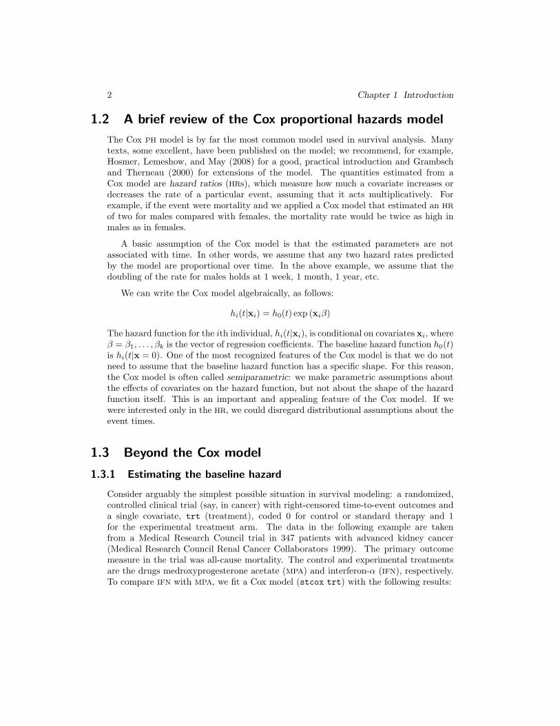
1.2 A brief review of the Cox proportional hazards model

The Cox PH model is by far the most common model used in survival analysis. Manytexts, some excellent, have been published on the model; we recommend, for example,Hosmer, Lemeshow, and May (2008) for a good, practical introduction and Grambschand Therneau (2000) for extensions of the model. The quantities estimated from aCox model are hazard ratios (HRs), which measure how much a covariate increases ordecreases the rate of a particular event, assuming that it acts multiplicatively. Forexample, if the event were mortality and we applied a Cox model that estimated an HR

of two for males compared with females, the mortality rate would be twice as high inmales as in females.

A basic assumption of the Cox model is that the estimated parameters are notassociated with time. In other words, we assume that any two hazard rates predictedby the model are proportional over time. In the above example, we assume that thedoubling of the rate for males holds at 1 week, 1 month, 1 year, etc.

We can write the Cox model algebraically, as follows:

hi(t|xi) = h0(t) exp (xiβ)

The hazard function for the ith individual, hi(t|xi), is conditional on covariates xi, whereβ = β1, . . . , βk is the vector of regression coefficients. The baseline hazard function h0(t)is hi(t|x = 0). One of the most recognized features of the Cox model is that we do notneed to assume that the baseline hazard function has a specific shape. For this reason,the Cox model is often called semiparametric: we make parametric assumptions aboutthe effects of covariates on the hazard function, but not about the shape of the hazardfunction itself. This is an important and appealing feature of the Cox model. If wewere interested only in the HR, we could disregard distributional assumptions about theevent times.

1.3 Beyond the Cox model

1.3.1 Estimating the baseline hazard

Consider arguably the simplest possible situation in survival modeling: a randomized,controlled clinical trial (say, in cancer) with right-censored time-to-event outcomes anda single covariate, trt (treatment), coded 0 for control or standard therapy and 1for the experimental treatment arm. The data in the following example are takenfrom a Medical Research Council trial in 347 patients with advanced kidney cancer(Medical Research Council Renal Cancer Collaborators 1999). The primary outcomemeasure in the trial was all-cause mortality. The control and experimental treatmentsare the drugs medroxyprogesterone acetate (MPA) and interferon-α (IFN), respectively.To compare IFN with MPA, we fit a Cox model (stcox trt) with the following results:

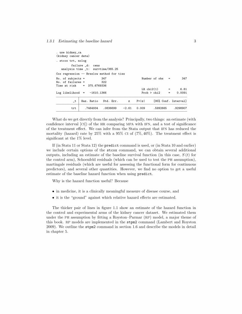
1.3.1 Estimating the baseline hazard 3

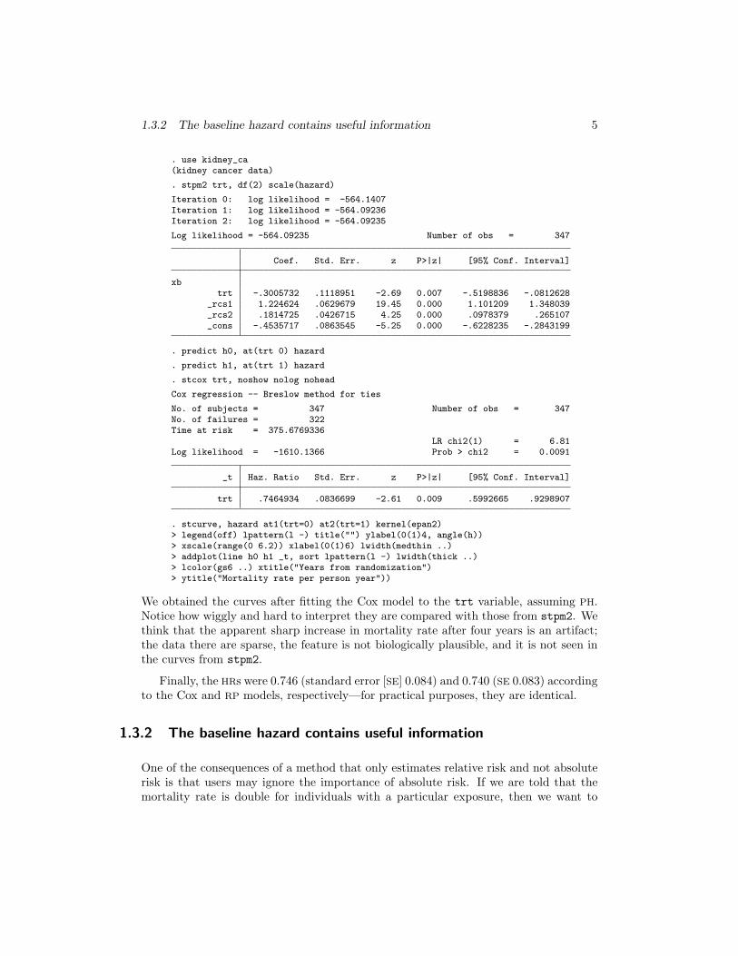
. use kidney_ca(kidney cancer data)

. stcox trt, nolog

failure _d: censanalysis time _t: survtime/365.25

Cox regression -- Breslow method for ties

No. of subjects = 347 Number of obs = 347No. of failures = 322Time at risk = 375.6769336

LR chi2(1) = 6.81Log likelihood = -1610.1366 Prob > chi2 = 0.0091

_t Haz. Ratio Std. Err. z P>|z| [95% Conf. Interval]

trt .7464934 .0836699 -2.61 0.009 .5992665 .9298907

What do we get directly from the analysis? Principally, two things: an estimate (withconfidence interval [CI]) of the HR comparing MPA with IFN, and a test of significanceof the treatment effect. We can infer from the Stata output that IFN has reduced themortality (hazard) rate by 25% with a 95% CI of (7%, 40%). The treatment effect issignificant at the 1% level.

If (in Stata 11 or Stata 12) the predict command is used, or (in Stata 10 and earlier)we include certain options of the stcox command, we can obtain several additionaloutputs, including an estimate of the baseline survival function (in this case, S (t) forthe control arm), Schoenfeld residuals (which can be used to test the PH assumption),martingale residuals (which are useful for assessing the functional form for continuouspredictors), and several other quantities. However, we find no option to get a usefulestimate of the baseline hazard function when using predict.

Why is the hazard function useful? Because

• in medicine, it is a clinically meaningful measure of disease course, and

• it is the “ground” against which relative hazard effects are estimated.

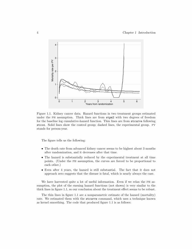
The thicker pair of lines in figure 1.1 show an estimate of the hazard function inthe control and experimental arms of the kidney cancer dataset. We estimated themunder the PH assumption by fitting a Royston–Parmar (RP) model, a major theme ofthis book. RP models are implemented in the stpm2 command (Lambert and Royston2009). We outline the stpm2 command in section 1.6 and describe the models in detailin chapter 5.


0

1

2

3

4

Mort

alit

y r

ate

per

PY

0 1 2 3 4 5 6Years from randomization

Figure 1.1. Kidney cancer data. Hazard functions in two treatment groups estimatedunder the PH assumption. Thick lines are from stpm2 with two degrees of freedomfor the baseline log cumulative-hazard function. Thin lines are from stcurve followingstcox. Solid lines show the control group; dashed lines, the experimental group. PY

stands for person-year.

The figure tells us the following:

• The death rate from advanced kidney cancer seems to be highest about 3 monthsafter randomization, and it decreases after that time.

• The hazard is substantially reduced by the experimental treatment at all timepoints. (Under the PH assumption, the curves are forced to be proportional toeach other.)

• Even after 4 years, the hazard is still substantial. The fact that it does notapproach zero suggests that the disease is fatal, which is nearly always the case.

We have harvested quite a lot of useful information. Even if we relax the PH as-sumption, the plot of the ensuing hazard functions (not shown) is very similar to thethick lines in figure 1.1, so our conclusion about the treatment effect seems to be robust.

The thin lines in figure 1.1 are a nonparametric estimate of the hazard (mortality)rate. We estimated them with the stcurve command, which uses a technique knownas kernel smoothing. The code that produced figure 1.1 is as follows:

1.3.2 The baseline hazard contains useful information 5

. use kidney_ca(kidney cancer data)

. stpm2 trt, df(2) scale(hazard)

Iteration 0: log likelihood = -564.1407Iteration 1: log likelihood = -564.09236Iteration 2: log likelihood = -564.09235

Log likelihood = -564.09235 Number of obs = 347

Coef. Std. Err. z P>|z| [95% Conf. Interval]

xbtrt -.3005732 .1118951 -2.69 0.007 -.5198836 -.0812628

_rcs1 1.224624 .0629679 19.45 0.000 1.101209 1.348039_rcs2 .1814725 .0426715 4.25 0.000 .0978379 .265107_cons -.4535717 .0863545 -5.25 0.000 -.6228235 -.2843199

. predict h0, at(trt 0) hazard

. predict h1, at(trt 1) hazard

. stcox trt, noshow nolog nohead

Cox regression -- Breslow method for ties

No. of subjects = 347 Number of obs = 347No. of failures = 322Time at risk = 375.6769336

LR chi2(1) = 6.81Log likelihood = -1610.1366 Prob > chi2 = 0.0091

_t Haz. Ratio Std. Err. z P>|z| [95% Conf. Interval]

trt .7464934 .0836699 -2.61 0.009 .5992665 .9298907

. stcurve, hazard at1(trt=0) at2(trt=1) kernel(epan2)> legend(off) lpattern(l -) title("") ylabel(0(1)4, angle(h))> xscale(range(0 6.2)) xlabel(0(1)6) lwidth(medthin ..)> addplot(line h0 h1 _t, sort lpattern(l -) lwidth(thick ..)> lcolor(gs6 ..) xtitle("Years from randomization")> ytitle("Mortality rate per person year"))

We obtained the curves after fitting the Cox model to the trt variable, assuming PH.Notice how wiggly and hard to interpret they are compared with those from stpm2. Wethink that the apparent sharp increase in mortality rate after four years is an artifact;the data there are sparse, the feature is not biologically plausible, and it is not seen inthe curves from stpm2.

Finally, the HRs were 0.746 (standard error [SE] 0.084) and 0.740 (SE 0.083) accordingto the Cox and RP models, respectively—for practical purposes, they are identical.

1.3.2 The baseline hazard contains useful information

One of the consequences of a method that only estimates relative risk and not absoluterisk is that users may ignore the importance of absolute risk. If we are told that themortality rate is double for individuals with a particular exposure, then we want to


know what reference value this doubling refers to. In a survival model, the referenceis usually the baseline hazard rate, which usually changes as a function of time. Thuseven if the PH assumption is reasonable, the impact of a particular exposure in absoluteterms depends on how long has passed since the time origin (diagnosis, randomization,start of treatment, etc.) and the magnitude of the underlying hazard rate.

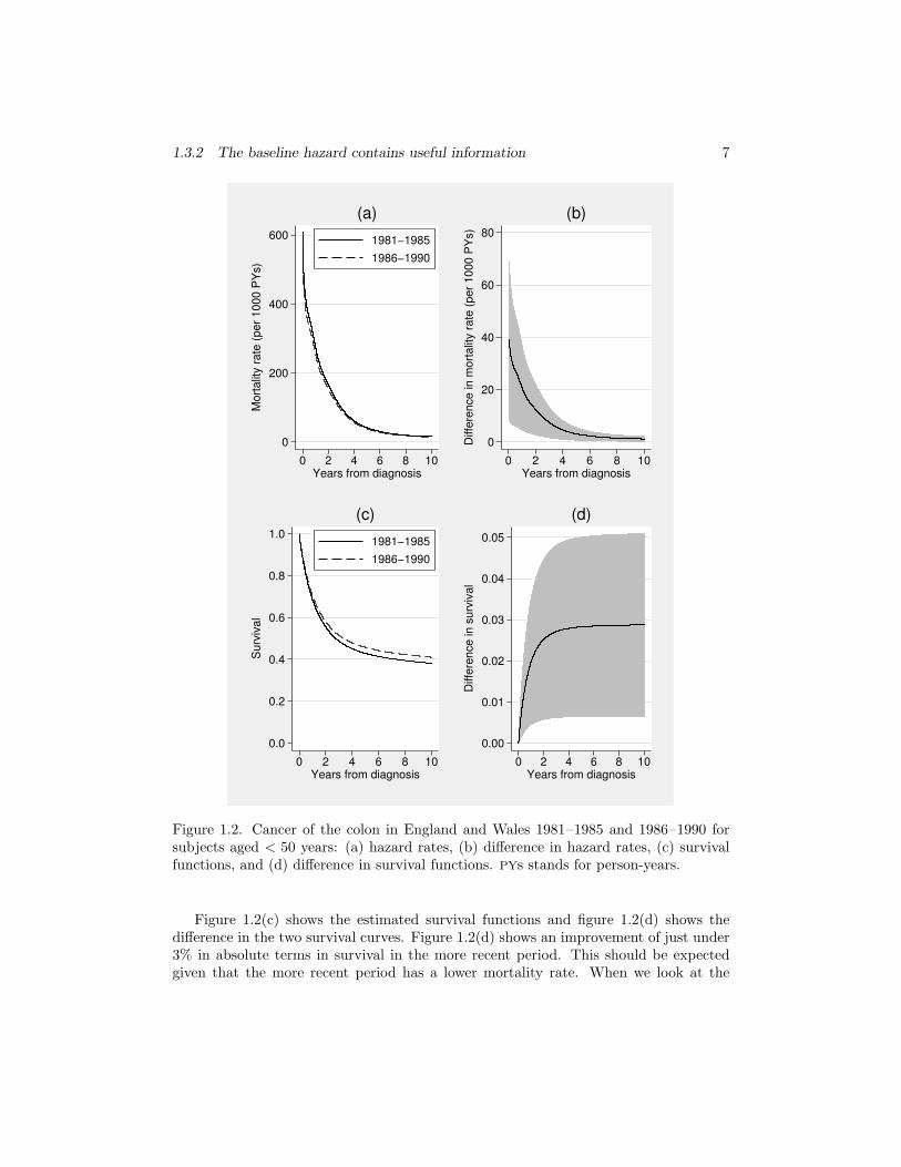
An example to illustrate the importance of the baseline hazard is in survival fromcolon cancer. Figure 1.2(a) shows data from England and Wales where the time fromdiagnosis to death from colon cancer in those ages < 50 years has been modeled andsmooth estimates of the hazard function derived for two time periods, 1981–1985 and1986–1990. The event is death from any cause and thus the hazard rate can be consid-ered as a mortality rate. The model assumes that the two hazard rates are proportional.The figure shows that the mortality rate is high in the first few months after diagnosis,but then decreases. By about 8 years, the mortality rate is very close to zero. We caninfer that very few colon cancer patients who have survived to this time will actually diebetween 8 and 10 years. When the mortality rate associated with a diagnosis of a par-ticular disease approaches zero, we have what is know as “statistical” or “population”cure (Lambert et al. 2007). The HR between the two time periods is 0.92, implying thatthe mortality rate is 8% lower in the more recent period. As the model assumes PH, theestimated relative effect is forced to be the same over the whole time period.

Figure 1.2(b) shows the difference in the hazard (mortality) rates. The absolute dif-ference decreases with increasing follow-up time. Thus the 8% reduction in the mortalityrate has little impact beyond about 6 years.

1.3.2 The baseline hazard contains useful information 7

0

200

400

600

Mort

alit

y r

ate

(per

1000 P

Ys)

0 2 4 6 8 10Years from diagnosis

1981−1985

1986−1990

(a)

0

20

40

60

80

Diffe

rence in m

ort

alit

y r

ate

(per

1000 P

Ys)


(b)

0.0

0.2

0.4

0.6

0.8

1.0

Surv

ival


1981−1985

1986−1990

(c)

0.00

0.01

0.02

0.03

0.04

0.05

Diffe

rence in s

urv

ival


(d)

Figure 1.2. Cancer of the colon in England and Wales 1981–1985 and 1986–1990 forsubjects aged < 50 years: (a) hazard rates, (b) difference in hazard rates, (c) survivalfunctions, and (d) difference in survival functions. PYs stands for person-years.

Figure 1.2(c) shows the estimated survival functions and figure 1.2(d) shows thedifference in the two survival curves. Figure 1.2(d) shows an improvement of just under3% in absolute terms in survival in the more recent period. This should be expectedgiven that the more recent period has a lower mortality rate. When we look at the


difference in the survival curves, we see that most of the improvement has been in thefirst 2–3 years.

We feel that the graphs shown in figure 1.2 give a better understanding of the diseaseand of the improvement in the more recent period than just quoting a hazard ratio of0.92.

1.3.3 Advantages of smooth survival functions

A Kaplan–Meier plot of the survival function, S (t), is an important feature of mostsurvival analyses and is widely presented in publications of applied work. For the Coxmodel, Stata’s predict command after stcox with the basesurv() option providesan estimate of the baseline survival function, S0 (t) = S (t|x = 0). From the baselinesurvival and the HR, we can predict the survival function for any combination of covariatevalues. However, all such survival functions are step functions and typically are notparticularly smooth. However, it is reasonable to suppose that the underlying functionis smooth. Also, the least precise parts of the curve get the most visual weight, a generalcriticism of Kaplan–Meier survival curves.

Kaplan–Meier-type estimates of S (t) are composed of a sequence of point estimatesof the survival function that are highly serially correlated. Accordingly, Kaplan–Meierplots tend to display “runs” of values that move away from and back toward the generaltrend, giving an undulating appearance. This may make the curve difficult to interpretand may lead to overemphasis of local features.

An example of these aspects, which is particularly a problem in smaller samples,appears in the kidney cancer data (see figure 1.3).

1.4.4 Relative survival 13

possible to define such an average HR, we doubt its usefulness, because the issue ofnoninterpretability remains. The HR is by definition a ratio of hazard functions. Forexample, a HR function that starts > 1 for small t and becomes < 1 for large t is notmeaningfully summarized by a single value near 1. We therefore regard the single HR

as a meaningless summary under nonproportional hazards unless the departures fromproportionality are so small as to be unimportant. We prefer to allow the HR to be afunction of time, as described for some of the models in chapters 5 and 7.

1.4 Why parametric models?

1.4.1 Smooth baseline hazard and survival functions

Parametric survival models generally provide smooth estimates of the hazard and sur-vival functions for any combination of covariate values. Exceptions are piecewisemodels—for example, the piecewise exponential (see section 4.3.1), for which the haz-ard function is a step function and the survival function has discontinuities in the firstderivative.

1.4.2 Time-dependent HRs

With parametric models, we can obtain essentially any type of output—for example, atime-dependent HR (see section 7.6)—as a function of the estimated model parameters(the covariates and time). Furthermore, we can use Stata’s powerful predictnl com-mand, which implements the delta method using numeric derivatives, to get SEs andCIs quite easily (see section 1.9).

1.4.3 Modeling on different scales

Sometimes, a covariate whose effect is nonproportional on the hazards scale may be(much closer to) proportional on another scale, such as the odds or probit (inversenormal probability) scales (see chapter 5). We may be able to take advantage of thedifferent possible scales to build a parsimonious and efficient alternative to a PH model.

1.4.4 Relative survival

In cancer survival, we often want to know the impact of covariates on the mortalityrate for a particular cancer. However, because cancer is usually a disease of old age,many people may die of diseases other than the cancer they were originally diagnosedwith. In relative survival models, we deal with this issue by incorporating expectedmortality, which we can usually obtain from routine data sources. Traditionally, simplepiecewise models have been used for relative survival, but all the advantages of standardparametric survival models also apply to relative survival models. See chapter 8 fordetails.


1.4.5 Prediction out of sample

The baseline survival function in a Cox model (estimated by predict varname,basesurv() following use of stcox) is available only in the estimation sample. Topredict survival outside the estimation sample, we need special measures, such as in-terpolation or even extrapolation. Using special measures limits the applications of theCox model in some situations. An important case arises when we wish to validate a sur-vival model in an independent sample, a task that necessitates out-of-sample prediction(see section 6.8).

1.4.6 Multiple time scales

In a Cox model, we can consider only one time scale—for example, time from diagnosisof disease or time from randomization in a clinical trial. Sometimes, for example, inage–period–cohort models (Clayton and Schifflers 1987), we might want to considermore than one time scale. See section 7.9 for an example of using multiple time scales.

1.5 Why not standard parametric models?

We have outlined some advantages of working with parametric models. In chapter 13of Cleves et al. (2010)—an excellent introduction to survival analysis in Stata—theauthors describe six standard parametric survival models—exponential, Weibull, Gom-pertz, lognormal, loglogistic, and generalized gamma. The models, together with a richset of extensions, are implemented in the portmanteau command streg. Cleves et al.(2010) give formulas for the hazard and survival functions for these models, togetherwith detailed examples and their implementation in Stata. We do not repeat the mate-rial here.

With such riches available, why do we need to go beyond streg? There are two mainreasons. First, the simpler parametric models in streg may not be flexible enough toadequately represent, say, the hazard function—in other words, they may not fit thedata well enough. (Concern about possible lack of fit of parametric models is one of themain reasons for the popularity of the Cox model; the shape of the baseline distributiondoes not influence estimates of HRs.) For example, the main parametric PH model, theWeibull, has a hazard function that always goes in the same direction with time—up,down, or constant. Many real-life datasets have hazards that peak after some period oftime and then decline, so the Weibull model can never fit such data well. Second, in ourbook, we present new classes of parametric models that include flexible PH models, butalso flexible proportional odds (PO) and probit-scale models. These alternative modelsgreatly extend the range of survival distributions that can be estimated.

1.5 Why not standard parametric models? 15

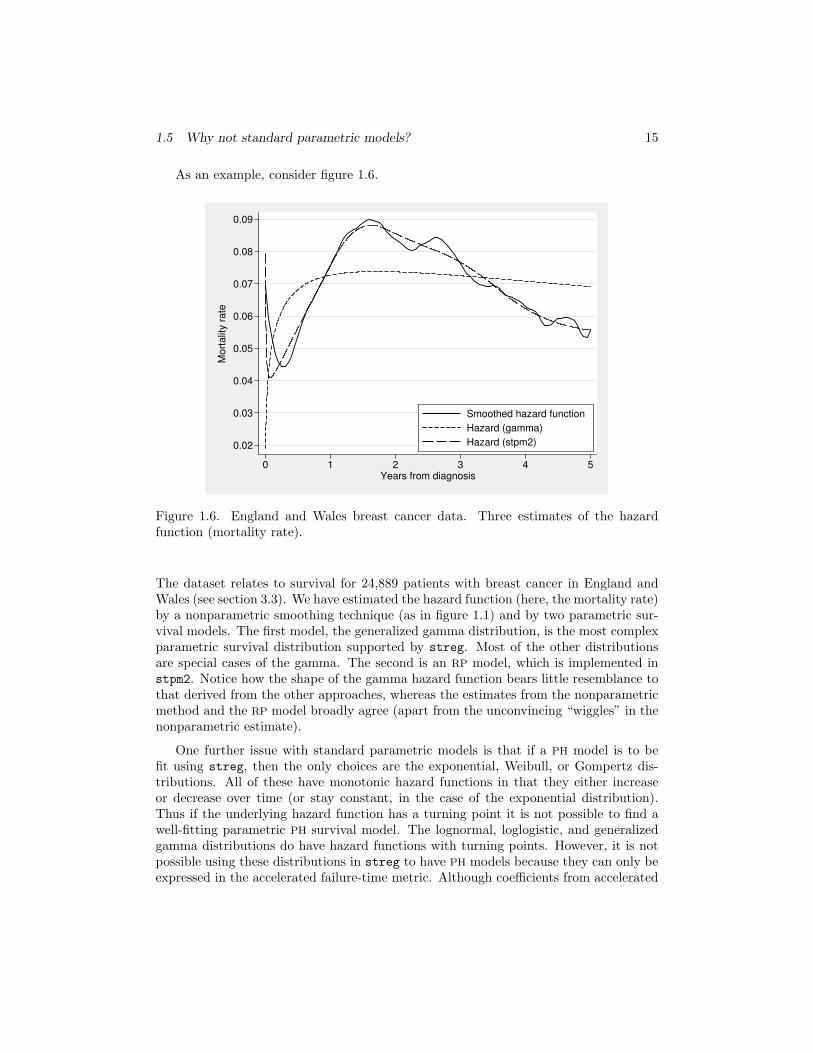
As an example, consider figure 1.6.

0.02

0.03

0.04

0.05

0.06

0.07

0.08

0.09M

ort

alit

y r

ate


Smoothed hazard function

Hazard (gamma)

Hazard (stpm2)

Figure 1.6. England and Wales breast cancer data. Three estimates of the hazardfunction (mortality rate).

The dataset relates to survival for 24,889 patients with breast cancer in England andWales (see section 3.3). We have estimated the hazard function (here, the mortality rate)by a nonparametric smoothing technique (as in figure 1.1) and by two parametric sur-vival models. The first model, the generalized gamma distribution, is the most complexparametric survival distribution supported by streg. Most of the other distributionsare special cases of the gamma. The second is an RP model, which is implemented instpm2. Notice how the shape of the gamma hazard function bears little resemblance tothat derived from the other approaches, whereas the estimates from the nonparametricmethod and the RP model broadly agree (apart from the unconvincing “wiggles” in thenonparametric estimate).

One further issue with standard parametric models is that if a PH model is to befit using streg, then the only choices are the exponential, Weibull, or Gompertz dis-tributions. All of these have monotonic hazard functions in that they either increaseor decrease over time (or stay constant, in the case of the exponential distribution).Thus if the underlying hazard function has a turning point it is not possible to find awell-fitting parametric PH survival model. The lognormal, loglogistic, and generalizedgamma distributions do have hazard functions with turning points. However, it is notpossible using these distributions in streg to have PH models because they can only beexpressed in the accelerated failure-time metric. Although coefficients from accelerated

Flexible Parametric Survival Analysis Using Stata: Beyond ... · book on survival analysis in Stata (Cleves et al. 2010): This is a book about survival analysis for the professional

Documents