Fin 3318 Chapter 8

1

Chapter 8 - An Introduction to Asset Pricing Models

Questions to be answered:• What are the assumptions of the capital asset

pricing model?• What is a risk-free asset and what are its risk-return

characteristics?• What is the covariance and correlation between the

risk-free asset and a risky asset or portfolio of risky assets?


• What is the expected return when you combine the risk-free asset and a portfolio of risky assets?

• What is the standard deviation when you combine the risk-free asset and a portfolio of risky assets?

• When you combine the risk-free asset and a portfolio of risky assets on the Markowitz efficient frontier, what does the set of possible portfolios look like?


• Given the initial set of portfolio possibilities with a risk-free asset, what happens when you add financial leverage (that is, borrow)?

• What is the market portfolio, what assets are included in this portfolio, and what are the relative weights for the alternative assets included?

• What is the capital market line (CML)? • What do we mean by complete diversification?

2


• How do we measure diversification for an individual portfolio?

• What are systematic and unsystematic risk?• Given the capital market line (CML), what is the

separation theorem?• Given the CML, what is the relevant risk measure

for an individual risky asset?• What is the security market line (SML) and how

does it differ from the CML?


• What is beta and why is it referred to as a standardized measure of systematic risk?

• How can you use the SML to determine the expected (required) rate of return for a risky asset?

• Using the SML, what do we mean by an undervalued and overvalued security, and how do we determine whether an asset is undervalued or overvalued?


• What is an asset’s characteristic line and how do you compute the characteristic line for an asset?

• What is the impact on the characteristic line when you compute it using different return intervals (e.g., weekly versus monthly) and when you employ different proxies (i.e., benchmarks) for the market portfolio (e.g., the S&P 500 versus a global stock index)?

3


• What happens to the capital market line (CML) when you assume there are differences in the risk-free borrowing and lending rates?

• What is a zero-beta asset and how does its use impact the CML?

• What happens to the security line (SML) when you assume transaction costs, heterogeneous expectations, different planning periods, and taxes?


• What are the major questions considered when empirically testing the CAPM?

• What are the empirical results from tests that examine the stability of beta?

• How do alternative published estimates of beta compare?

• What are the results of studies that examine the relationship between systematic risk and return?


• What other variables besides beta have had a significant impact on returns?

• What is the theory regarding the “market portfolio” and how does this differ from the market proxy used for the market portfolio?

• Assuming there is a benchmark problem, what variables are affected by it?

4

Capital Market Theory:An Overview

• Capital market theory extends portfolio theory and develops a model for pricing all risky assets

• Capital asset pricing model (CAPM) will allow you to determine the required rate of return for any risky asset

Assumptions of Capital Market Theory

1. All investors are Markowitz efficient investors who want to target points on the efficient frontier. – The exact location on the efficient frontier and,

therefore, the specific portfolio selected, will depend on the individual investor’s risk-return utility function.


2. Investors can borrow or lend any amount of money at the risk-free rate of return (RFR). – Clearly it is always possible to lend money at

the nominal risk-free rate by buying risk-free securities such as government T-bills. It is not always possible to borrow at this risk-free rate, but we will see that assuming a higher borrowing rate does not change the general results.

5


3. All investors have homogeneous expectations; that is, they estimate identical probability distributions for future rates of return.– Again, this assumption can be relaxed. As long

as the differences in expectations are not vast, their effects are minor.


4. All investors have the same one-period time horizon such as one-month, six months, or one year. – The model will be developed for a single

hypothetical period, and its results could be affected by a different assumption. A difference in the time horizon would require investors to derive risk measures and risk-free assets that are consistent with their time horizons.


5. All investments are infinitely divisible, which means that it is possible to buy or sell fractional shares of any asset or portfolio. – This assumption allows us to discuss

investment alternatives as continuous curves. Changing it would have little impact on the theory.

6


6. There are no taxes or transaction costs involved in buying or selling assets. – This is a reasonable assumption in many

instances. Neither pension funds nor religious groups have to pay taxes, and the transaction costs for most financial institutions are less than 1 percent on most financial instruments. Again, relaxing this assumption modifies the results, but does not change the basic thrust.


7. There is no inflation or any change in interest rates, or inflation is fully anticipated.– This is a reasonable initial assumption, and it

can be modified.


8. Capital markets are in equilibrium.– This means that we begin with all investments

properly priced in line with their risk levels.

7


• Some of these assumptions are unrealistic• Relaxing many of these assumptions would

have only minor influence on the model and would not change its main implications or conclusions.

• A theory should be judged on how well it explains and helps predict behavior, not on its assumptions.

Risk-Free Asset

• An asset with zero standard deviation• Zero correlation with all other risky assets• Provides the risk-free rate of return (RFR)• Will lie on the vertical axis of a portfolio

graph

Covariance with a Risk-Free Asset

Covariance between two sets of returns is

∑=

=n

1ijjiiij )]/nE(R-)][RE(R-[RCov

Because the returns for the risk free asset are certain,

0RF =σ Thus Ri = E(Ri), and Ri - E(Ri) = 0

Consequently, the covariance of the risk-free asset with any risky asset or portfolio will always equal zero. Similarly the correlation between any risky asset and the risk-free asset would be zero.

8

Combining a Risk-Free Asset with a Risky Portfolio

Expected returnthe weighted average of the two returns

))E(RW-(1(RFR)W)E(R iRFRFport +=

This is a linear relationship


Standard deviationThe expected variance for a two-asset portfolio is

211,22122

22

21

21

2port rww2ww)E( σσσσσ ++=

Substituting the risk-free asset for Security 1, and the risky asset for Security 2, this formula would become

iRFiRF σσσσσ iRF,RFRF22

RF22

RF2port )rw-(1w2)w1(w)E( +−+=

Since we know that the variance of the risk-free asset is zero and the correlation between the risk-free asset and any risky asset i is zero we can adjust the formula

22RF

2port )w1()E( iσσ −=


Given the variance formula22

RF2port )w1()E( iσσ −=

22RFport )w1()E( iσσ −=the standard deviation is

iσ)w1( RF−=

Therefore, the standard deviation of a portfolio that combines the risk-free asset with risky assets is the linear proportion of the standard deviation of the risky asset portfolio.

9


Since both the expected return and the standard deviation of return for such a portfolio are linear combinations, a graph of possible portfolio returns and risks looks like a straight line between the two assets.

Portfolio Possibilities Combining the Risk-Free Asset and Risky Portfolios on the Efficient Frontier

)E( portσ

)E(R port Exhibit 8.1

RFR

MC

AB

D

Risk-Return Possibilities with Leverage

To attain a higher expected return than is available at point M (in exchange for accepting higher risk)

• Either invest along the efficient frontier beyond point M, such as point D

• Or, add leverage to the portfolio by borrowing money at the risk-free rate and investing in the risky portfolio at point M

10

Portfolio Possibilities Combining the Risk-Free Asset and Risky Portfolios on the Efficient Frontier

)E( portσ

)E(R port

Exhibit 8.2

RFR

M

CML

Borrowing

Lending

The Market Portfolio

• Because portfolio M lies at the point of tangency, it has the highest portfolio possibility line

• Everybody will want to invest in Portfolio M and borrow or lend to be somewhere on the CML

• Therefore this portfolio must include ALL RISKY ASSETS


Because the market is in equilibrium, all assets are included in this portfolio in proportion to their market value

11


Because it contains all risky assets, it is a completely diversified portfolio, which means that all the unique risk of individual assets (unsystematic risk) is diversified away

Systematic Risk

• Only systematic risk remains in the market portfolio

• Systematic risk is the variability in all risky assets caused by macroeconomic variables

• Systematic risk can be measured by the standard deviation of returns of the market portfolio and can change over time

Examples of Macroeconomic Factors Affecting Systematic Risk

• Variability in growth of money supply• Interest rate volatility• Variability in

– industrial production– corporate earnings– cash flow

12

How to Measure Diversification

• All portfolios on the CML are perfectly positively correlated with each other and with the completely diversified market Portfolio M

• A completely diversified portfolio would have a correlation with the market portfolio of +1.00

Diversification and the Elimination of Unsystematic Risk

• The purpose of diversification is to reduce the standard deviation of the total portfolio

• This assumes that imperfect correlations exist among securities

• As you add securities, you expect the average covariance for the portfolio to decline

• How many securities must you add to obtain a completely diversified portfolio?

Diversification and the Elimination of Unsystematic Risk

Observe what happens as you increase the sample size of the portfolio by adding securities that have some positive correlation

13

Number of Stocks in a Portfolio and the Standard Deviation of Portfolio Return

Exhibit 8.3Standard Deviation of Return

Number of Stocks in the Portfolio

Standard Deviation of the Market Portfolio (systematic risk)

Systematic Risk

Total Risk

Unsystematic (diversifiable) Risk

The CML and the Separation Theorem

• The CML leads all investors to invest in the M portfolio

• Individual investors should differ in position on the CML depending on risk preferences

• How an investor gets to a point on the CML is based on financing decisions

• Risk averse investors will lend part of the portfolio at the risk-free rate and invest the remainder in the market portfolio


Investors preferring more risk might borrow funds at the RFR and invest everything in the market portfolio

14


The decision of both investors is to invest in portfolio M along the CML (the investment decision)

M

CML

PFR

B

A

( )portE R

portσ


The decision to borrow or lend to obtain a point on the CML is a separate decision based on risk preferences (financing decision)


Tobin refers to this separation of the investment decision from the financing decision, the separation theorem

15

A Risk Measure for the CML

• Covariance with the M portfolio is the systematic risk of an asset

• The Markowitz portfolio model considers the average covariance with all other assets in the portfolio

• The only relevant portfolio is the M portfolio

A Risk Measure for the CML

Together, this means the only important consideration is the asset’s covariance with the market portfolio

A Risk Measure for the CMLBecause all individual risky assets are part of the M portfolio, an

asset’s rate of return in relation to the return for the M portfolio may be described using the following linear model:

ε++= Miiiit RbaRwhere:

Rit = return for asset i during period t

ai = constant term for asset i

bi = slope coefficient for asset i

RMt = return for the M portfolio during period t

= random error termε

16

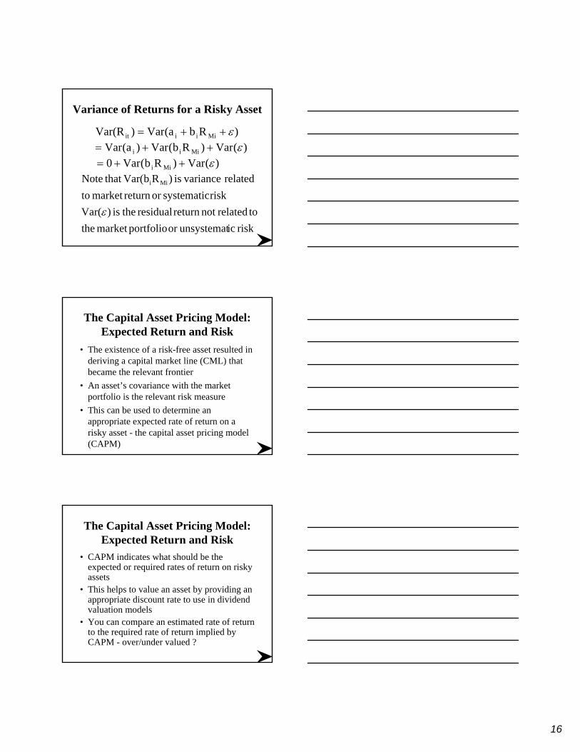
Variance of Returns for a Risky Asset

)Rba(Var)Var(R Miiiit ε++=)(Var)Rb(Var)a(Var Miii ε++=

)(Var)Rb(Var0 Mii ε++=

risk icunsystemator portfoliomarket the torelatednot return residual theis )(Var

risk systematicor return market to related varianceis )Rb(Var that Note Mii

ε

The Capital Asset Pricing Model: Expected Return and Risk

• The existence of a risk-free asset resulted in deriving a capital market line (CML) that became the relevant frontier

• An asset’s covariance with the market portfolio is the relevant risk measure

• This can be used to determine an appropriate expected rate of return on a risky asset - the capital asset pricing model (CAPM)

The Capital Asset Pricing Model: Expected Return and Risk

• CAPM indicates what should be the expected or required rates of return on risky assets

• This helps to value an asset by providing an appropriate discount rate to use in dividend valuation models

• You can compare an estimated rate of return to the required rate of return implied by CAPM - over/under valued ?

17

The Security Market Line (SML)

• The relevant risk measure for an individual risky asset is its covariance with the market portfolio (Covi,m)

• This is shown as the risk measure• The return for the market portfolio should

be consistent with its own risk, which is the covariance of the market with itself - or its variance: 2

mσ

Graph of Security Market Line (SML)

)E(R i

Exhibit 8.5

RFR

imCov2mσ

mR

SML

The Security Market Line (SML)The equation for the risk-return line is

)Cov(RFR-RRFR)E(R Mi,2M

Mi σ

+=

RFR)-R(Cov

RFR M2M

Mi,

σ+=

2M

Mi,Covσ

We then define as beta

RFR)-(RRFR)E(R Mi iβ+=

)( iβ

18

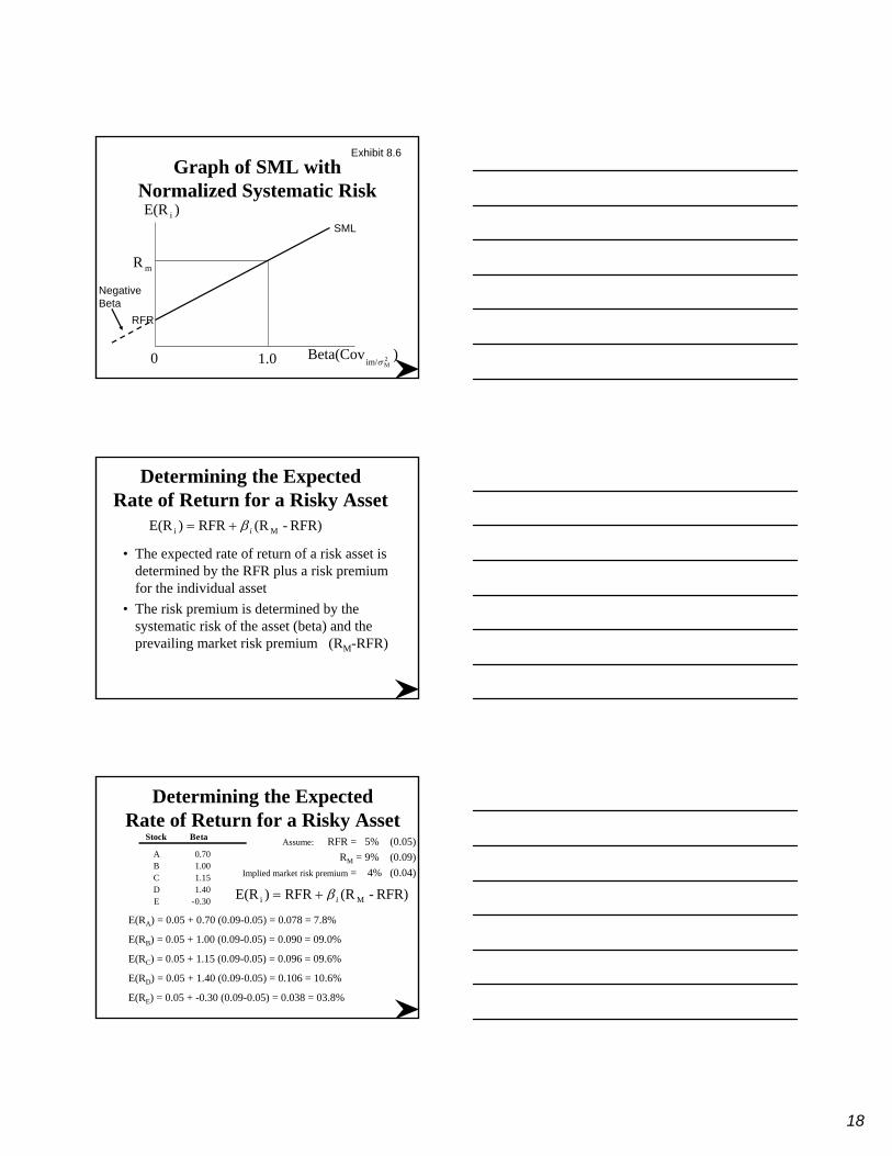
Graph of SML with Normalized Systematic Risk

)E(R i

Exhibit 8.6

)Beta(Cov 2Mim/σ0.1

mR

SML

0

Negative Beta

RFR

Determining the Expected Rate of Return for a Risky Asset

• The expected rate of return of a risk asset is determined by the RFR plus a risk premium for the individual asset

• The risk premium is determined by the systematic risk of the asset (beta) and the prevailing market risk premium (RM-RFR)

RFR)-(RRFR)E(R Mi iβ+=


Assume: RFR = 5% (0.05) RM = 9% (0.09)

Implied market risk premium = 4% (0.04)

Stock Beta

A 0.70B 1.00C 1.15D 1.40E -0.30 RFR)-(RRFR)E(R Mi iβ+=

E(RA) = 0.05 + 0.70 (0.09-0.05) = 0.078 = 7.8%

E(RB) = 0.05 + 1.00 (0.09-0.05) = 0.090 = 09.0%

E(RC) = 0.05 + 1.15 (0.09-0.05) = 0.096 = 09.6%

E(RD) = 0.05 + 1.40 (0.09-0.05) = 0.106 = 10.6%

E(RE) = 0.05 + -0.30 (0.09-0.05) = 0.038 = 03.8%

19


• In equilibrium, all assets and all portfolios of assets should plot on the SML

• Any security with an estimated return that plots above the SML is underpriced

• Any security with an estimated return that plots below the SML is overpriced

• A superior investor must derive value estimates for assets that are consistently superior to the consensus market evaluation to earn better risk-adjusted rates of return than the average investor

Identifying Undervalued and Overvalued Assets

• Compare the required rate of return to the expected rate of return for a specific risky asset using the SML over a specific investment horizon to determine if it is an appropriate investment

• Independent estimates of return for the securities provide price and dividend outlooks

Calculating Systematic Risk: The Characteristic Line

The systematic risk input of an individual asset is derived from a regression model, referred to as the asset’s characteristic line with the model portfolio:

εβα ++= tM,iiti, RRwhere: Ri,t = the rate of return for asset i during period tRM,t = the rate of return for the market portfolio M during t

miii R-R βα =

2M

Mi,Covσ

β =i

error term random the=ε

20

The Impact of the Time Interval• Number of observations and time interval used in

regression vary• Value Line Investment Services (VL) uses weekly

rates of return over five years• Merrill Lynch, Pierce, Fenner & Smith (ML) uses

monthly return over five years• There is no “correct” interval for analysis• Weak relationship between VL & ML betas due to

difference in intervals used• The return time interval makes a difference, and

its impact increases as the firm’s size declines

The Effect of the Market Proxy• The market portfolio of all risky assets must

be represented in computing an asset’s characteristic line

• Standard & Poor’s 500 Composite Index is most often used– Large proportion of the total market value of

U.S. stocks– Value weighted series

Weaknesses of Using S&P 500as the Market Proxy

– Includes only U.S. stocks – The theoretical market portfolio should include

U.S. and non-U.S. stocks and bonds, real estate, coins, stamps, art, antiques, and any other marketable risky asset from around the world

21

Relaxing the Assumptions• Differential Borrowing and Lending Rates

– Heterogeneous Expectations and Planning Periods

• Zero Beta Model– does not require a risk-free asset

• Transaction Costs– with transactions costs, the SML will be a band

of securities, rather than a straight line

Relaxing the Assumptions

• Heterogeneous Expectations and Planning Periods– will have an impact on the CML and SML

• Taxes– could cause major differences in the CML and

SML among investors

Empirical Tests of the CAPM• Stability of Beta

– betas for individual stocks are not stable, but portfolio betas are reasonably stable. Further, the larger the portfolio of stocks and longer the period, the more stable the beta of the portfolio

• Comparability of Published Estimates of Beta

– differences exist. Hence, consider the return interval used and the firm’s relative size

22

Relationship Between Systematic Risk and Return

• Effect of Skewness on Relationship– investors prefer stocks with high positive

skewness that provide an opportunity for very large returns

• Effect of Size, P/E, and Leverage– size, and P/E have an inverse impact on returns

after considering the CAPM. Financial Leverage also helps explain cross-section of returns

Relationship Between Systematic Risk and Return

• Effect of Book-to-Market Value– Fama and French questioned the relationship

between returns and beta in their seminal 1992 study. They found the BV/MV ratio to be a key determinant of returns

• Summary of CAPM Risk-Return Empirical Results– the relationship between beta and rates of return

is a moot point

The Market Portfolio: Theory versus Practice

• There is a controversy over the market portfolio. Hence, proxies are used

• There is no unanimity about which proxy to use• An incorrect market proxy will affect both the beta

risk measures and the position and slope of the SML that is used to evaluate portfolio performance

23

Summary

• The assumption of capital market theory expand on those of the Markowitz portfolio model and include consideration of the risk-free rate of return

Summary

• The dominant line is tangent to the efficient frontier– Referred to as the capital market line (CML)– All investors should target points along this line

depending on their risk preferences

Summary• All investors want to invest in the risky

portfolio, so this market portfolio must contain all risky assets– The investment decision and financing decision

can be separated– Everyone wants to invest in the market

portfolio– Investors finance based on risk preferences

24

Summary• The relevant risk measure for an individual

risky asset is its systematic risk or covariance with the market portfolio– Once you have determined this Beta measure

and a security market line, you can determine the required return on a security based on its systematic risk

Summary

• Assuming security markets are not always completely efficient, you can identify undervalued and overvalued securities by comparing your estimate of the rate of return on an investment to its required rate of return

Summary

• When we relax several of the major assumptions of the CAPM, the required modifications are relatively minor and do not change the overall concept of the model.

25

Summary

• Betas of individual stocks are not stable while portfolio betas are stable

• There is a controversy about the relationship between beta and rate of return on stocks

• Changing the proxy for the market portfolio results in significant differences in betas, SMLs, and expected returns

Summary

• It is not possible to empirically derive a true market portfolio, so it is not possible to test the CAPM model properly or to use model to evaluate portfolio performance

What is Next?

• Alternative asset pricing models

26

The InternetInvestments Online

http://www.valueline.comhttp://www.wsharpe.comhttp://gsb.uchicago.edu/fac/eugene.fama/http://www.moneychimp.com

Future topicsChapter 9

• Multifactor Models of Risk and Return

Fin 3318 Chapter 8

Documents