Exploring future changes in smallholder farming systems by ... · 1 Exploring future changes in smallholder farming systems by linking socio-economic ... We discuss the results in

1

Exploring future changes in smallholder farming systems by linking socio-economic 1

scenarios with regional and household models 2

3

Mario Herrero1*

, Philip K. Thornton2,3

, Alberto Bernués4, Isabelle Baltenweck

3, Joost 4

Vervoort2,5

, Jeannette van de Steeg3, Stella Makokha

6, Mark T. van Wijk

3, Stanley 5

Karanja3, Mariana C. Rufino

3 and Steven J. Staal

3 6

7

1Commonwealth Scientific and Industrial Research Organisation, 306 Carmody Road, St 8

Lucia, 4067 QLD, Australia 9

2CGIAR Research Programme on Climate Change, Agriculture and Food Security 10

(CCAFS), PO Box 30709-00100, Nairobi, Kenya 11

3International Livestock Research Institute (ILRI), PO Box 30709-00100, Nairobi, Kenya 12

4AgriFood Research and Technology Centre of Aragon, Avda. Montaña 930, 50059 – 13

Zaragoza, Spain 14

5Environmental Change Institute, University of Oxford, OX1 3QY, UK 15

6Kenyan Agricultural Research Institute (KARI), Nairobi, Kenya 16

17

18

*Corresponding author: Dr Mario Herrero, CSIRO, 306 Carmody Road, St Lucia, 19

4067, QLD, Australia, email: [email protected]; tel +61 7 3214 2538. 20

21

22

23

24

25

26

27

28

29

30

31

2

Abstract 1

2

We explore how smallholder agricultural systems in the Kenyan highlands might 3

intensify and/or diversify in the future under a range of socio-economic scenarios. Data 4

from approximately 3000 households were analysed and farming systems characterized. 5

Plausible socio-economic scenarios of how Kenya might evolve, and their potential 6

impacts on the agricultural sector, were developed with a range of stakeholders. We study 7

how different types of farming systems might increase or diminish in importance under 8

different scenarios using a land-use model sensitive to prices, opportunity cost of land 9

and labour, and other variables. We then use a household model to determine the types of 10

enterprises in which different types of households might engage under different socio-11

economic conditions. Trajectories of intensification, diversification, and stagnation for 12

different farming systems are identified. Diversification with cash crops is found to be a 13

key intensification strategy as farm size decreases and labour costs increase. Dairy 14

expansion, while important for some trajectories, is mostly viable when land available is 15

not a constraint, mainly due to the need for planting fodders at the expense of cropland 16

areas. We discuss the results in relation to induced innovation theories of intensification. 17

We outline how the methodology employed could be used for integrating global and 18

regional change assessments with local-level studies on farming options, adaptation to 19

global change, and upscaling of social, environmental and economic impacts of 20

agricultural development investments and interventions. 21

22

23

Keywords 24

25

Scenarios, smallholders, household modeling, land use modeling, sustainable 26

intensification, agriculture, dairy 27

28

29

30

1. Introduction 31

3

1

The role that smallholder agricultural producers are likely to play in global food 2

production and food security in the coming decades is highly uncertain. In many parts of 3

the tropics, particularly sub-Saharan Africa, smallholder production is critical to the food 4

security of the poor. Industrialisation of agricultural production is occurring in many 5

places, largely in response to burgeoning demand for food. Some smallholders may be 6

able to seize the opportunities that exist and develop, and operate as sustainable and 7

profitable smallholder agricultural production systems (Herrero et al., 2010; Thornton, 8

2010). Whether large numbers of smallholders will be able to do this in a carbon-9

constrained global economy and in an environment characterised by a changing climate 10

and by increased climatic variability, will depend on many things such as increasing 11

regulation, building social protection and strengthening links to urban areas, and 12

substantial investment in agriculture (Wiggins, 2009; World Bank, 2009). Understanding 13

how smallholder systems may evolve in the future is critical if poverty alleviation and 14

food security goals are to be achieved. 15

In many parts of the tropics, particularly Africa and Asia, smallholders operate 16

mixed crop-livestock systems, which integrate different enterprises on the farm; crops 17

provide food for consumption and for cash sales, as well as residues to feed livestock, and 18

livestock provide draft power to cultivate the land and manure to fertilise the soil. These 19

systems are often highly diversified, and the synergies between cropping and livestock 20

keeping offer real opportunities for raising productivity and increasing resource use 21

efficiency (Herrero et al., 2010). Whether these systems can increase household incomes 22

and enhance the availability of and access to food for rapidly increasing urban 23

populations in the coming years, while at the same time maintaining environmental 24

services, is a question of considerable importance. 25

Studying this question requires some consideration of theories of change. A 26

general model of agricultural intensification originated with Boserup (1965), who 27

described it as an endogenous process responding to increased population pressure. As 28

the ratio of land to population decreases, farmers are induced to adopt technologies that 29

raise returns to land at the expense of a higher input of labour. The direct causal factor is 30

relative factor price changes, in accordance with the theory of induced innovation. At 31

4

low human population densities, production systems are extensive, with high availability 1

of land and few direct crop-livestock interactions. Population increases lead to increases 2

in demand for crop and livestock products, which in turn increases the value of manure 3

and feed resources and other inputs, leading to increased crop and livestock productivity. 4

As population increases yet further, systems intensify through specialisation or 5

diversification in production as relative values of land, labour and capital continue to 6

change: fertilizer replaces manure, tractors replace draft animals, concentrate feeds 7

replace crop residues, and cash crops replace food crops (Baltenweck et al., 2003). 8

Other factors can also play a significant role in determining the nature and 9

evolution of crop-livestock systems (McIntire et al., 1992). In humid areas with a high 10

disease challenge for large ruminants, crop-livestock interactions are likely to be limited 11

owing to lower livestock densities. Other factors include economic opportunities, cultural 12

preferences, climatic variability (e.g., droughts that lead to livestock losses), lack of 13

capital to purchase animals, and labour bottlenecks at some periods of the year that may 14

prevent farmers from adopting technologies such as draft power (Powell and Williams, 15

1993). Nevertheless, common patterns of both the drivers and the outcomes of 16

intensification of tropical crop-livestock systems can be identified. Choice of crops and 17

livestock interventions have been shown to be at least partly dependent on relative labour 18

and land costs and on market access, at a wide range of sites throughout the tropics 19

(Baltenweck et al., 2003). Furthermore, in the same study education level, market access 20

and human population densities were shown to be major drivers of crop-livestock 21

systems intensification (Baltenweck et al., 2003). 22

At the same time, alongside these larger scale drivers of farm development, the 23

ability of smallholders to implement new practices is further determined by intrinsic 24

system properties that may act as modifiers to their adoption. Farmers’ objectives and the 25

rules governing labour allocation and gender differentiation in the household are 26

examples (Thornton and Herrero, 2001; Waithaka et al., 2006). Such factors are not 27

necessarily related to spatial or macro-economic drivers; they therefore need to be studied 28

at the farm household level. 29

30

To understand the evolution of smallholder crop-livestock systems, we propose that. 31

5

these systems should be examined at multiple levels by analysing and linking macro-level 1

socio-economic drivers, regional-level land-use patterns, and micro-level household 2

dynamics and strategies. Complementary methods should be used that appropriately 3

reflect the key dynamics of each of these levels (Cash et al., 2006). The significant 4

complexity and uncertainty associated with the interacting biophysical and socio-5

economic dimensions of agricultural systems should be taken into account by using a 6

multiple scenarios approach, informed by relevant stakeholder perspectives (Biggs et al., 7

2007). Interactions of smallholder systems with changing contexts should be simulated 8

and discussed iteratively with key stakeholders to explore longer-term evolutionary 9

pathways (Kinzig, 2006). 10

11

In this paper we provide an example of this multi-level, multi-scenario, evolutionary 12

framework for the analysis of smallholder systems, using complementary modeling 13

approaches and harnessing relevant stakeholder perspectives. We build on the work of 14

Baltenweck et al. (2003) and Herrero et al. (2007a) by studying the potential household-15

level impacts of crop-livestock intensification using crop-dairy systems data obtained 16

from longitudinal monitoring of representative case studies and key informants 17

(extension officers and policy makers) from Kenya. The objective of the study was to 18

generate socio-economic development scenarios as to how crop-livestock systems in the 19

highlands of Kenya might evolve in the next two decades and evaluate these plausible, 20

alternative futures through a multi-level modeling framework that includes a) the 21

development of scenarios providing different socio-economic conditions at the country 22

level and above; b) a regional land-use change analysis projecting the spatial distribution 23

of farming systems into the future; and c) the use of a household model to evaluate the 24

results of the spatial analysis at the farm level, allowing for a deeper understanding of 25

internal farm dynamics. We conclude with a discussion of the value of multi-scale, 26

stakeholder-generated, iterative analyses in evaluating synergies and trade-offs in farming 27

systems, particularly related to the dynamics of global change in tropical smallholder 28

systems. 29

30

6

2. Materials and methods 1

2

2.1 Area of Study 3

4

The study area, which covers the highlands of Kenya is, approximately 65,000 km2 5

spread over 34 districts (figure 1). The human population in the area has increased from 6

approximately 21 to 26 million people in the last several years (Kenya Government, 7

2002; Kenya National Bureau of Statistics, 2010), representing about 68% of the Kenyan 8

human population. Most people in the study area live in the rural areas. The region in 9

Kenya is representative of many regions in sub-Saharan Africa with a similar climate and 10

with similar scenarios for their socio-economic development, e.g. potentially increased 11

economic growth in the rural areas with connections to the rapidly developing urban 12

centers while still uncertainty remains about the supportiveness of the political and policy 13

environment for these developments (e.g. southern Uganda). As such results of this 14

analysis in terms of the driving factors behind changes and the constraints limiting 15

economic growth in the smallholder farming sector can be seen as representative for large 16

areas in the east African highlands. 17

18

Figure 1 about here 19

20

The soils are predominantly deep, well-drained strongly weathered tropical soils 21

(Nitosols and Andosols) and suited for growing tea, coffee, and wheat as cash crops. 22

Maize and beans are the predominant staple food crops. Compared with the lowlands, the 23

highlands of Kenya have a more favorable agro-ecology for dairy and crop production 24

and better market opportunities because of the high population numbers with a tradition 25

for consuming milk (Staal et al., 2001; Waithaka et al., 2000). 26

The area has a diversity of farming systems, varying from subsistence farmers, 27

farmers with major dairy activities, intensified farmers with limited dairy activities, and 28

export cash crop farmers with limited or major dairy activities. Production in the Kenyan 29

Highlands is often based on the close integration of dairy cattle into the crop production 30

(Bebe et al., 2003). In the study area, production is typically conducted on a few acres, 31

7

with a herd of crossbred cows ranging from 1 to 5 in size (usually Friesian or Ayrshire 1

crossed with local Zebu). Crops (for food and cash) are often integrated with dairy 2

production to diversify risks from dependency on a single crop or livestock enterprise. 3

Dairy production is part of the farming system to produce milk for subsistence and for 4

sale, to produce manure for supporting crop production, to provide dairy animals for 5

savings and for social status (Waithaka et al., 2006). Mixed farming derives 6

complementarities in resource use: crop residues and by-products from crop production 7

constitute feeds for cattle, which return manure to maintain soil fertility and crop 8

production, allowing sustained multiple cropping (Giller et al., 2006; Herrero et al., 9

2010). 10

11

2.2 Overview of Methodological Framework 12

13

The methodological framework of the research is represented in Figure 2. This 14

framework combines complementary analytical perspectives: socio-economic conditions 15

at the country level through scenarios, a regional/sub-national level simulating spatial 16

land use changes, and a representation of choices and strategies at the household level. 17

The various approaches are linked through the scenario analysis, so that both the spatial 18

dynamics of farming systems and patterns of system evolution at the household level can 19

be studied under similar scenario assumptions. 20

21

Figure 2 about here 22

23

Based on surveys of 2866 households, farming systems were characterized into 24

six groups. These farming systems were used as input for both spatial and household 25

modeling. These household data were obtained from three surveys conducted in central 26

and western Kenya between 1996 and 2000, as part of a collaborative effort to 27

characterize smallholder dairy systems from the Kenyan Ministry of Livestock 28

Development & Fisheries, the Kenya Agricultural Research Institute (KARI), and the 29

International Livestock Research Institute (ILRI) (http://www.smallholderdairy.org/). 30

8

A household questionnaire was completed through single interviews with the 1

household head or in his/her absence, the most senior member available or the household 2

member responsible for the farm. The questionnaires were divided into sections covering 3

household composition, labour availability and use; farm activities and facilities; 4

livestock inventory; cattle feeding, dairying with emphasis on milk production and milk 5

marketing; livestock management and health services; household income and sources; 6

and cooperative membership and milk consumption. Along with the survey data, each 7

surveyed household was geo-referenced. 8

The households were grouped using an expert-based classification using the 9

following criteria: i) cultivation of only food crops or cash crops for the local market or 10

cultivation of cash crops for export; ii) level of external inputs, captured by the extent of 11

inorganic fertilizer used and an area with fertilizer below or higher than 25% of the 12

cropped area; and iii) level of milk production, captured by cattle milk density, below or 13

above 1000 l milk per ha per year. Figure 3 presents the rationale behind the 14

classification. 15

16

Figure 3 about here 17

18

2.3 Socio-economic scenarios developed with regional experts 19

20

Different socio-economic environments modulate how farming systems may 21

evolve in the future under different sets of policy and demographic conditions. These 22

conditions are complex, uncertain, and linked across global, (sub)continental and national 23

levels. To adequately capture the notion that smallholder farmers might face significantly 24

different futures, we developed scenarios. Scenarios are a set of alternate narratives in 25

words and/or numbers that describe plausible ways in which the future might unfold (van 26

Notten et al., 2003; Kok et al., 2007). Scenarios can be viewed as a linking tool that 27

integrates qualitative narratives or stories about the future and quantitative formulations 28

based on formal modeling (Alcamo, 2008; Volkery et al., 2008) . As such, scenarios 29

enhance our understanding of how systems work, behave and evolve, and so can help in 30

the assessment of future developments under alternative policy directions (Kok et al., 31

9

2011). In this case study, scenarios were also used to connected different levels of 1

analysis by exploring smallholder developments under similar assumptions and socio-2

economic conditions. 3

The recognition that socio-economic systems are complex and uncertain and may 4

offer widely diverse challenges to smallholders prompts the need for the involvement of 5

stakeholders with long expertise from different sectors, such as policy or the private 6

sector, in the focus region (Wilkinson and Eidinow, 2008). The involvement of such 7

stakeholders also makes it more likely that researchers ask appropriate and locally 8

relevant questions (Xiang and Clarke, 2003). In the case of our study, three scenarios 9

were adapted based on the inputs from planners, policy makers, researchers and 10

organizations interested in Kenya’s future agricultural development during several 11

meetings and stakeholders’ workshops. More details can be found in Van de Steeg et al. 12

(2007). 13

Prompted by these stakeholders, we used Kenya’s Economic Recovery Strategy 14

for Wealth and Employment Creation (ERSP) scenario (Kenyan Government, 2003) as 15

an explicitly normative, desired scenario for the region that focuses on equitable rural 16

development. However, the stakeholder engagement also yielded two less optimistic 17

scenarios: a scenario where development largely fails, and a scenario where inequitable 18

growth dominates. We refer to these scenarios as the “equitable growth”, “baseline ” (= 19

low growth) and “inequitable growth” scenarios, respectively. 20

The projected growth trends for the coming 20 year assumed under the different 21

scenarios, described in Table 1, were translated into new spatial data layers for the drivers 22

of the spatial analysis; for the farm level analysis, scenarios were translated via 23

modifying different parameters and restrictions in the household model. Table 1 describes 24

the various assumptions made for these scenarios. The resulting temporal data layers are 25

called dynamic data layers here, as opposed to static data layers which are assumed not to 26

be affected by the different scenarios. 27

28

Table 1 about here 29

30

10

The equitable growth storyline describes the future of Kenya with both political and 1

economic reform, and represents the outcomes planned under the Economic Recovery 2

Strategy for Wealth and Employment Creation. The policy and institutional environments 3

are characterized by functioning institutions and policies, and strong capable oversight 4

institutions to address issues to support economic growth. There is a strong commitment 5

to market-based solutions in order to obtain an optimum balance between demand and 6

supply of goods, services and environmental quality at national and international levels. 7

Under this scenario the Economic Recovery Strategy for Wealth and Employment 8

Creation is fully and successfully implemented. Efficient policy institutions contribute to 9

the enhancement of the agricultural sector. Expected rates of growth and investment as 10

presented in the Economic Recovery Strategy for Wealth and Employment Creation 11

official documents are used to quantify the changes in the spatial data layers over time. 12

The baseline (= low growth) scenario describes the future of Kenya with 13

inefficient institutions, and a failure to address slow economic growth, unemployment 14

and poverty. The political dilemma is characterized by poor policy formulation and 15

weakness of oversight institutions, such as parliament, to create a favorable policy 16

environment. In this scenario, Kenya continues to slide into ‘the abyss of 17

underdevelopment and hopelessness’ (Kenya Government, 2003) as no attempts are 18

undertaken for economic recovery. The political environment contributes to the 19

deterioration or at best stagnation of the agricultural sector. Past trends are used to 20

quantify the dynamic spatial data layers under consideration. 21

The inequitable growth storyline describes the future of Kenya with inefficient 22

institutions and inequitable economic growth. Economic growth is localized, brought 23

about by initiatives of individuals and the private sector, with limited facilitation by the 24

government. Market development and infrastructure are relatively good only in areas 25

with export-led agriculture. In these areas agriculture technology development is also 26

strong, mostly focused on cost reductions and yield increases. There is an increase in 27

agricultural productivity in the large-scale production of cash crops for the international 28

market. In these areas there are local off-farm income opportunities available for rural 29

people via wage labour in commercial farming, with some rural development and income 30

multiplier effects. Under this scenario the Economic Recovery Strategy for Wealth and 31

11

Employment Creation is only partly implemented and not all Kenyans benefit, 1

particularly not smallholders. 2

3

12

2.4 Spatial Analysis Model 1

A specific farming system is expected to occur at locations with conditions that best fit 2

that type of farming system at that moment in time. Logit models were used to predict the 3

relative probability for the different farming systems at a certain location and at a certain 4

time, with the farming systems as dependent variable and location characteristics as 5

explanatory variables (Van de Steeg et al, 2010). The explanatory variables considered in 6

the analysis are chosen based on the analysis described in Staal et al. (2002), by linking 7

spatial measures to the perceived real decision-makers, thus matching the spatial and 8

behavioural units. 9

10

The mapping of the spatial distribution of farming systems is described in Van de Steeg 11

et al (2010). Linking farming system choice and drivers of change is a key element of this 12

research effort. Based on the biophysical and socio-economic conditions of a location, the 13

fitted logit models were used to calculate the probabilities of finding different farming 14

systems across the study area. The individual probability maps for the different farming 15

systems were combined into an overall map indicating the spatial distribution of farming 16

systems given the relative probabilities and the region-wide prevalence, by means of an 17

iterative procedure (Verburg et al., 2002). A simple classification by assigning the 18

location to the farming system with the highest probabilities is not appropriate, as this 19

would reflect the prevalence of farming systems in the original sampling which is not 20

representative for the entire study area. Instead, the allocated area of each farming system 21

is determined by an estimate of the surface area of each farming system type occurring in 22

the study area. The distribution of farming systems, at the base year, is derived from an 23

external database (CBS, 1997) that was considered to contain a representative sample for 24

determining the prevalence of the different farming systems. 25

26

Over time, the surface area of different farming systems is determined by the demand for 27

certain agricultural commodities, i.e. how much of each agricultural commodity is 28

required to satisfy the needs of the changing population. We considered the four most 29

important commodities for the study area; maize, beans, tea and milk. Using the initial 30

13

estimate of the surface area and the total demand for the commodities based on 1

FAOSTAT, the percentage of production of each commodity supplied by each farming 2

system is estimated. 3

4

Next, using average consumption data, growth in gross domestic product (GDP) per 5

capita under the different scenarios, and income elasticity of the demand for four 6

commodities, the evolution of the demand for the different commodities by year and by 7

scenario is predicted. Consumption data were derived from FAOSTAT. Income elasticity 8

demands were derived from USDA (2013); we used 0.58, 0.81, 0.9 and 1.6 for maize, 9

beans, milk and tea respectively. We assumed a growth in gross domestic product per 10

capita of 0.7%, 4.7%, and 2.7% for the low, equitable and inequitable growth scenario 11

respectively (Kenya Government, 2002; Kenya Government, 2003). 12

13

Based on the evolution in the demand for commodities, it is possible to predict the 14

change in farming systems, using the contribution of each farming system to the 15

production of the different commodities (under the assumption of similar productivity by 16

cluster). The map with farming systems distribution at the base year, the set of static and 17

dynamic spatial data layers, and the logit models that relate the probability of occurrence 18

of farming systems to location characteristics were used as input to a spatial and temporal 19

model of farming systems dynamics. Scenario analyses were performed with the CLUE-S 20

(the Conversion of Land Use and its Effects at Small regional extent) modelling 21

framework. CLUE-S is specifically developed for the spatially explicit simulation of 22

land-use and farming system change based on an empirical analysis of location suitability 23

combined with the dynamic simulation of competition and interactions between the 24

spatial and temporal dynamics of land-use systems (Verburg et al., 2002). 25

26

Based on the demand for certain commodities, i.e. an estimate of the prevalence of the 27

different farming systems, the predicted probabilities are corrected in an iterative 28

procedure to obtain a classification that reflects the prevalence correctly as well as the 29

relative probabilities calculated for the different locations. For farming system types 30

14

where the allocated area is smaller than the demanded area the value of the iteration 1

variable is increased. For land use types for which too much is allocated the value is 2

decreased. Through this procedure it is possible that the local suitability based on the 3

location factors is overruled by the iteration variable due to the differences in regional 4

demand. The procedure followed balances the bottom-up allocation based on location 5

suitability and the top-down allocation based on regional demand. 6

For each scenario a sequence of maps with the spatial distribution of farming systems 7

over time was generated following the method described above. From this we were able 8

to simulate the trajectories of farming systems change for each scenario. 9

10

2.5 Household Modelling 11

12

Clustering Procedure for Household Characterization 13

14

In order to identify case studies that could have diverse pathways of evolution inside each 15

predetermined class (see Figure 3), a further classification of farms was performed and 16

each class was further divided into three sub-groups representing the variability within 17

each class. 18

From the variables of the initial dataset, those that could change over time included land 19

size, cropped area, level of education of farmer, milk production, herd size, and family 20

size. Rather than grouping the farms using a cluster analysis on these variables, a 21

Principal Component Analysis was first performed by class in order to observe if there 22

were relationships between these variables and to check that the same factors could be 23

identified in each of the six classes, i.e. the importance of variables when explaining 24

heterogeneity was similar between classes. 25

Factor 1 in the Principal Component Analysis was Farm Size (a combination of 26

land and herd size) for all classes. Other factors were defined by only one variable 27

(Family Size, Milk Production and Education Level) and changed relative positions 28

depending on the class. With these factors obtained from the Principal Component 29

Analysis, a hierarchical cluster analysis (by predetermined class) was performed using 30

Ward’s method of aggregation. Non-hierarchical clustering and other methods of 31

15

aggregation were also tested but results were less satisfactory as resulting sub-clusters 1

were unbalanced. To improve clustering performance and avoid distortion from outliers, 2

these were eliminated from the analysis using the TRIM option of Statistical Analysis 3

System (SAS, 2001). The final clustering process resulted in the definition of the same 6 4

classes as in the expert opinion exercise (Figure 3), but now with three sub-groups in 5

each of these classes systematically representing the diversity within each class. . 6

7

Description of Case Study Households 8

9

From the final 18 household groups (six classes and three sub-groups in each), a 10

representative case study farm was selected. The IMPACT household characterization 11

tool (Herrero et al., 2007b) was used to collect detailed information from each case study 12

household on general system characteristics (location, system type, agro-climatology, for 13

example); land management (crops and fodders planted, growing seasons, for example); 14

livestock and their management (species, animal numbers, feeding systems); household 15

composition and farm labour; and inputs and outputs (cash, labour, food, nutrients, stock 16

and other assets). 17

18

IMPACT analysis and subsequent household model analysis were performed for each of 19

the 18 case studies. Here, because of the large quantity of results produced (18 case 20

studies by three scenarios by four periods of time), only three contrasting case study 21

households will be presented.. These are heterogeneous in terms of size, structure and 22

orientation of production. The three case studies correspond to the following: 1. 23

Subsistence farm with dairy (class 2: food crops or cash crops for domestic market only, 24

no or low external inputs and high dairy); 2. Intensified farm with dairy (class 4: food 25

crops or cash crops for domestic market only, high external inputs and high dairy); 3. 26

Export oriented farm with dairy (class 6: cash crops for export, high dairy). 27

IMPACT also computed a range of simple indicators of farming systems in terms 28

of monthly cash flows, the family’s monthly nutritional status, annual soil nutrient 29

balance, and labour use efficiency (Herrero et al., 2007b). The main characteristics of the 30

three case studies are shown in Table 2. 31

16

1

1. Subsistence farm with dairy. 2

3

The household consists of eight members (five of them working on the farm). Farm size 4

is 2.46 ha (only 18.7% owned), from which 2 ha are pastures, mostly cut-and-carry 5

pastures. The only crops in this farm are maize and beans. Fertilizer and hybrid seeds are 6

used but in very low amounts. Labour is hired to meet additional requirement for feeding 7

cattle, planting, weeding and harvesting. The herd structure consists of three female 8

calves, four cows, one young bull and one reproductive male, which is used for serving 9

farmers’ cows in the area, bringing some income to the farm. The breed of cattle kept is 10

Friesian and the major purpose is milk production. The cattle are zero-grazed all year 11

round and are fed on Napier grass, maize stover and concentrates. 12

The main source of income for the family is the sale of milk; very little surplus of 13

food crops is sold. The household also gets some off-farm income (20.8% of total 14

household income) by doing wage work on other farms. The household’s major costs are 15

related to food crop production, with comparatively few livestock costs and other 16

expenses (off-farm food, children, school fees, etc.). Annual income per person and per 17

ha are medium in relation to the other case studies. 18

Most energy and protein sources come from the food crops and milk produced on 19

the farm, but the family is not able to meet the World Health Organisation energy 20

requirements (deficit of 11.6% of total family requirements). 21

22

Table 2 about here 23

24

2. Intensified farm with dairy. 25

26

This household consists of seven members (four working on the farm). Farm size 27

is 1.4 ha (43% owned), from which 0.4 ha is dedicated to crops and the rest to grazing 28

pastures. The major crops are maize, beans, bananas and kales. The main cash crop is 29

kale, although some beans and bananas are also sold. Fertilizer is mostly used on maize 30

and pesticides are applied to kale. One Ayrshire cow and its calf are kept for milk 31

17

production. They graze on communal land and are also stall-fed with Napier grass, crop 1

residues and concentrates. 2

Most agricultural income for the household comes from kale and some milk. 3

Some off-farm income is obtained through wages received from work on other farms by 4

the household head and his wife, accounting for 18.8% of total household income. 5

Livestock keeping costs are more important than those due to agriculture, because of little 6

hiring of labour for cropping activities. Economic results are the poorest of the three case 7

studies. 8

Similar to the previous case study, most energy and protein sources come from 9

the food crops and milk produced on the farm, and the family is nearly able to meet the 10

WHO energy requirements (deficit of 1.3% of total family requirements). 11

12

3. Export-oriented farm with dairy. 13

14

This household consists of six members (four working on the farm). The household head 15

has twelve years of education. Farm size is the biggest of all the case studies with 4.8 ha 16

(all owned), from which 3.7 ha is dedicated to crops and the rest to cut-and-carry 17

pastures. Main crops are for export (tea, coffee and passion fruit) and the other crops 18

(beans, maize and potato) are for family consumption. Casual labour is hired to meet the 19

requirements of land preparation, planting, weeding and harvesting. Fertilizer, pesticides 20

and hybrid seeds are used in substantial quantities. This household keeps highly improved 21

Friesian cattle (two calves, two heifers, one young bull and four milking cows). A long-22

term labourer has been hire to take care of the cattle. The system of feeding is zero-23

grazing, with Napier grass, crop residues, concentrates and brewers by-products. 24

The only household income comes from agriculture and milk, the last being 25

slightly more important than export crops. Livestock keeping costs are comparatively 26

low in relation to the costs of cropping (casual labour and inputs). Economic results -27

globally, per person and per ha - are the best of the three case studies. 28

This family is able to meet largely its World Health Organisation energy and 29

protein requirement, and contrary to what was observed in the previous case studies, the 30

18

main source of food is purchased, although only a low proportion (6.8%) of total income 1

is spent in purchasing food. 2

3

Household Modelling 4

5

The IMPACT tool was linked to a household linear programming model and used to 6

generate the data files that this model needed to run (Herrero et al., 2007b). The 7

Household model allows the identification of the optimal combination of activities to 8

achieve an objective function subject to the constraints of the system. It is based on a 9

linear programming optimization model developed in Xpress-MP. The household model 10

structure and functioning are presented briefly below; further details can be found in the 11

supplementary information. 12

13

The objective function was to maximize farm gross margin: crop sales + livestock sales 14

+ other income – crops inputs – livestock inputs – labour – food purchase – other 15

expenses. 16

17

The decision variables in the household model included the following. Land use 18

(management options for plots). Dairy orientation (optimal number of dairy cows). 19

Feeding strategies for cows and herd structure, these are not optimized and only the 20

observed current situation is considered. Therefore, observed milk production per cow is 21

constant. Use of commodities (eaten by the family, sell, buy, store, feed the animals, 22

leave as fertilizer). 23

24

Some key constraints were related to food security (food needs by the family in each 25

month), seasonal labour availability, cost and demand; seasonal prices, market demand, 26

food storage, the range of cropping and livestock activities; and annual cash flows, which 27

are essential for investing in new activities or for dealing with specific cash demands at 28

certain periods during the year. 29

30

19

The household model developed by Herrero and Fawcett (2002) and used in previous 1

modeling studies in smallholder systems (Waithaka et al., 2006; Gonzalez Estrada et al., 2

2008; Zingore et al., 2009) was further adapted for multi-time period modeling, running 3

in monthly periods in steps of five years from 2005 to 2025 (see supplementary 4

information for the description of the model). Optimization occurs annually, and results 5

from the previous year were used as the starting point for the next year. Additional 6

activities such as new cropping options could be included in the household model, 7

allowing the farming systems to change orientation of production or intensify. 8

Trajectories of change were defined through a transition matrix (Table 3) to allow 9

one type of system to evolve through time into another, and this could occur after one run 10

of five years – for instance, a farmer could evolve from being a subsistence farmer to 11

become a farmer growing cash crops and/ or having more intensive dairy production. The 12

transition matrix constitutes a logical “roadmap” of how a system might evolve into 13

another as time progresses, and this roadmap is different for the different scenarios 14

defined above. With this approach we add a degree of realism to systems’ change. 15

16

Table 3 about here 17

18

To translate the drivers described in Table 1, which define the trajectories described in 19

Table 3, into the information requirements of the household model, projections of 20

different variables that changed according to scenario, specific location of the case study 21

and period of time were carried out. These related specifically to land size and 22

opportunity cost of labour, as it was considered that these two variables were most 23

directly affected by the projected demographic and off-farm employment projections in 24

the alternative scenarios (Baltenweck et al., 2003). Real values of land size and cost of 25

labour and projections through time are represented in Figure 4. We assume changes in 26

crop and livestock production due to climate change in the time window up to 2025 are 27

small compared to the socio-economic changes that are represented here, i.e. price 28

changes and changes in land size. 29

Figure 4 about here 30

31

20

Several assumptions had to be made to run the household model. These are described 1

below. 2

3

Assumptions on intensification trajectories: transition from subsistence farming 4

systems to intensified systems was simulated through an increase in the use of fertilizers 5

and expected yield improvement for the major food and cash crops: maize, beans and 6

potato. The DSSAT models (Jones et al., 2003) were used to produce fertilizer response 7

curves for these main crops. 8

Assumptions on export-oriented trajectories: to simulate transition of cash- and 9

food-oriented farming systems to export oriented farms, a new cropping option was 10

introduced, that of growing passion fruit. According to the stakeholders consulted and the 11

Kenya Agricultural Research Institute, this is a promising cash crop in the Kenyan 12

highlands. For the new cropping option, information on yearly requirements of inputs 13

(fertilizers, pesticides, etc.) and labour on a monthly basis, establishment costs, yields, 14

and prices were obtained from Kenya Agricultural Research Institute scientists and other 15

expert opinion. 16

The first trajectory considers changes in labour cost and land size, and values of 17

these two driving forces are different by scenarios to mimic the scenarios narratives. The 18

values of these two variables by scenario are presented in Figure 4. Under the first 19

trajectory, the number of cows is also a decision variable. Compared with the first 20

trajectory, the second trajectory considers change in labour costs and land size, and the 21

number of cows is still a decision variable; in addition, the model is set to choose whether 22

to start growing passion fruit and whether to intensify crop production (captured by 23

applying fertilizer on the maize and beans plots). 24

25

Figure 4 around here 26

27

Assumptions of simulations across 20 years: to run the household model for a 28

period of 20 years, four periods of five years each were considered, and optimisations 29

were done annually. The final output obtained from one period in terms of optimal land 30

use and number of cows was used as the initial conditions for the next period. To do this, 31

21

non-annual costs (for example, establishment cost of crops or cost of purchasing new 1

cows) were divided by five. 2

When running the household model for the case study households with observed 3

data, calibration of the model for specific constraints was needed. Although the 4

household model has quite an elaborate set of constraints, they are still somewhat generic 5

and cannot reflect farmer behavior exactly; and they may not reflect specific local 6

conditions, such as limited amounts of inputs being available due to local market 7

restrictions, for example. Therefore, a process of calibration of some model constraints 8

was carried out. This usually involved modifying the market prices of some commodities 9

to reflect the internal transaction costs incurred by the household. When results of the 10

household model came near the observed results in the farm, the specific model (called 11

‘optimal base’ in the results shown below) constituted the starting point for subsequent 12

runs. 13

We did not perform a systematic sensitivity analyses for each of the case studies, 14

but in this study the scenario analyses, with its diverse socio-economic pathways provide 15

substantial parameter variability to understand how farming systems are likely to evolve 16

under different conditions. Similar observations were made recently by Claessens et al. 17

(2012).. Scenarios were analysed for three different farm types, for different input 18

settings and over three periods of time, and the results obtained in this analyses show 19

which drivers, variables and parameters captured in this setup are most important in 20

driving changes in the functioning of the farm households. This methodology also 21

determines whether the household model is sensitive enough for detecting change caused 22

by the socio-economic scenarios (see Figure 4) against this background of substantial 23

variability. 24

25

3. Results 26

27

3.1 Spatial Modelling 28

29

3.1 Spatial Modelling 30

22

In order to map the spatial distribution of farming systems over time, first the surface area 1

demanded by certain agricultural commodities of the different farming systems is 2

determined for the base year (Van de Steeg et al., 2010). Table 4 presents the percentage 3

of production of certain agricultural commodities supplied by each farming system. Note 4

that farming system classes two and four were combined, since the number of households 5

in these two categories was very small. The last category represents the non–agricultural 6

households. 7

8

Table 4 about here 9

10

The evolution of the demand for the different commodities by year and by scenario is 11

predicted. Table 5 summarizes the demand for the different commodities 12

(tons/year/person). 13

14

Table 5 about here 15

16

The combined annual changes in the demand for different commodities (Table 5) will 17

change the surface area of the different farming systems (Table 4) accordingly. Table 6 18

provides the estimates of the distribution of farming systems over time, driven by the 19

evolution in the demand for commodities. 20

21

Table 6 about here 22

23

Based on the evolution in the demand for commodities, it is possible to predict the spatial 24

trajectories in farming systems. Farming systems change is found all over the study area 25

(Figure 5), but especially in the neighbourhood of urban areas where population density 26

is high and where there are many possibilities for off-farm income generation. Besides 27

demand, changes in farming systems are also driven by the variability of the spatial 28

variables (Table 1). As spatial variables are changing over time, the optimal occurrence 29

of a certain farming system for a given location will change (Table 7). Consequently, a 30

reallocation of land takes place between farming systems. Between 15 to 25% of the 31

23

study area is likely to change for the different scenarios (Figure 5), and this range is used 1

as the basis for defining the three scenario storylines that are the outcomes of the CLUE-2

S model exercise. 3

4

Figure 5 about here 5

6

The preference for certain farming systems for a specific location is determined by 7

several household and spatial variables. It is not possible to derive a dominant 8

explanatory factor that leads to the change of one farming systems to another at a regional 9

level. The trajectories of farming systems change constitute a complex system driven by 10

many household and location characteristics, both static and dynamic. 11

12

Table 5 about here 13

14

Baseline scenario 15

About 20% of the surface area of the study area was projected to change in this scenario, 16

so the midrange value of the predicted range is shown in Figure 5. Of this, more than 17

50% of the farming systems change into export-oriented farming systems. Most 18

important trajectories of change were from subsistence and intensified farmers with 19

limited dairy activities to export cash crop farming with limited dairy activities. 20

21

Equitable growth scenario 22

About 25% of the surface area of the study area was projected to change for this scenario, 23

the highest value of the range predicted in Figure 5. Of this, more than 61% of the 24

farming systems changed into export-oriented farming systems. Also for this scenario the 25

most important trajectories of change were from subsistence and intensified farmers with 26

limited dairy activities to export cash crop farming with limited dairy activities. 27

28

Inequitable growth scenario 29

About 15% of the surface area of the study area was projected to change for this scenario, 30

the lowest value of the range predicted in Figure 5. Of this, more than 40% of the farming 31

24

systems changed into export-oriented farming systems in the zone without large-scale 1

farming, and about 25% in the zone with large-scale farming. For this scenario the most 2

important trajectories of change were intensified farmers with limited dairy activities to 3

export cash crop farming with limited dairy activities, and from export cash crop farmers 4

with limited dairy activities to intensified farming or non-agricultural activities. 5

6

3.2 Household Modelling 7

8

Results are presented for three case studies (Figures 6, 7 and 8) under the different 9

scenarios, for a time horizon of 20 years (in five-year periods, results of 2005-2010 and 10

2020-2025 are presented) and for one or two trajectories of change, as described in Table 11

4. Observed data, the optimal solution “optimal base scenario” after the fine tuning 12

process, under the current circumstances in terms of input/ output prices, land area and 13

labour availability, and the results of the scenarios are also presented in Figures 6, 7 and 14

8. 15

16

Evolution of the Case Studies 17

18

Subsistence with dairy (Figure 6): This case study is defined by a medium size family 19

with intermediate land area (2.46 ha) and relatively large herd size. The “optimal base 20

scenario” indicates maintenance of milk production and concentration on production of 21

maize and beans. 22

In the baseline scenario, in combination with Trajectory 1, dairy declines 23

gradually from period 1 through 4 from eight cows in the first period to five cows in the 24

last period, due to decreasing land size that reduces land availability for food crops and 25

cut-and-carry forage. Hired labour decreases drastically and there is a higher dependency 26

of the household on basic off-farm staple food and forages. 27

In Trajectory 2, dairy declines drastically in the first five years and then remains 28

constant as from the second period; this occurs because the farmer starts to grow passion 29

fruits that are more profitable than dairy. With decreasing land size over time, however, 30

the farmer has to decrease the land allocated to this enterprise in the subsequent periods. 31

25

In this scenario, the farmer increases the land under maize intercropped with beans, 1

which suggests a move towards increased farming for subsistence food crops (the farmer 2

intensifies the crop activities by applying fertilizer on the maize-beans plot) and at the 3

same time starts to export crops to improve economic output. Hired labour evolves 4

following the requirements of the passion fruit crop. Other results of the model, not 5

shown here, were that the dependency on off-farm staple food decreases, and the 6

dependency on purchased forages increases. 7

Under the “equitable growth” scenario, the farmer maintains the dairy herd due to 8

land consolidation (the farmer can allocate more land to fodder), despite the increase in 9

labour costs that could have potentially negatively influenced the decision to keep cattle. 10

The biggest change in land use is the proportion of land dedicated to maize and beans, 11

with the aim of improving food security in the household and selling the surplus. Hired 12

labour increases due to the larger cropping area. 13

In Trajectory 2, the number of cows on the farm decreases in the first period (due 14

to substitution of forage area for passion fruit), but the number increases again afterwards 15

when land area enlarges. It is important to notice that the farmer only starts growing 16

passion fruit if cash is available to start this activity, which has high initial costs. Cash is 17

also available to use fertilizer on the maize-beans plot. In the first period there is a higher 18

dependency on off-farm staple food and forage, but decreases in the second and third 19

periods. Hired labour use increases largely due to the cultivation of passion fruit. 20

In the “inequitable growth” scenario, with labour costs and land size values being 21

“intermediate”, the results of the household model are also in between those observed in 22

the other two scenarios. Trajectory 1 is stable and similar to the “optimal base” (land 23

remains constant). In Trajectory 2, the number of cows decreases drastically as the farmer 24

chooses to grow passion fruit, taking up land at the expense of planted fodder. More land 25

is also allocated to maize and beans where fertilizer is applied to increase yields. 26

27

Figure 6 about here 28

29

Intensified with dairy (Figure 7): This case study also refers to a smallholder farmer but 30

now with a high proportion of off-farm income. The “optimal base scenario” slightly 31

26

increases the amount of land used for food and cash crops (maize and beans) at the 1

expense of the grassland area, but maintains the dairy activity. 2

Under the baseline scenario and Trajectory 1, the dairy herd is maintained from 3

the first to the fourth period despite the decline in grazing resources due to the decrease in 4

land holdings (through increases in the purchase of Napier grass forage). There is no 5

major change in the cropping patterns under this trajectory, except that the kale cropping 6

area doubles to generate more cash. 7

In Trajectory 2, when passion fruit is an option, the farmer starts the activity (cash 8

is available from previous periods) and decreases the land for dairy (cut-and-carry forage 9

and natural pastures), thereby reducing herd size in the last period. Fewer food crops are 10

grown (maize intercropped with beans and bananas), together with less area for kale in 11

the final period. No additional fertilizer is applied. Therefore, there is a higher 12

dependency on off-farm staple food and forage. Hired labour needs to be increased to 13

deal with the requirements of passion fruit. 14

The results obtained in the “equitable growth” scenario are similar to those in the 15

baseline scenario. This can be explained by the fact that land size increases marginally for 16

this farmer. It is worth noting that some land is left unallocated during the last period of 17

the second trajectory, suggesting that high costs of labour under this scenario prevented 18

the farmer from increasing high labour-intensive activities such as dairy or passion fruit 19

production. 20

The evolution of the trajectories under the “inequitable growth” scenario shows 21

similar results to the previous scenario except that the farmer maintains his dairy herd 22

even when growing passion fruit. This is explained by the fact that under this scenario the 23

cost of labour increases less than in the equitable scenario; and only a marginal part of the 24

land is left unallocated. 25

26

Figure 7 about here 27

28

Export oriented with dairy: This case study involves the biggest farm (4.8 ha) and the one 29

with the highest diversification of activities (dairy and several export crops). All income 30

comes from the farm and the profit obtained is the largest of all the case studies. The 31

27

“optimal base simulation” slightly increases the amount of land dedicated to export crops 1

(coffee) at the expense of grassland and planted fodder. A large amount of food is 2

purchased from outside the farm (maize and bananas). 3

It is important to notice that, due to the peri-urban location of the farm, close to 4

the capital city Nairobi where population densities are higher and where there is a higher 5

demand for land for non-agricultural activities, the evolution of land size is opposite to 6

that observed for the other case studies. This means there are increases in land size in the 7

baseline scenario and decreases in the “equitable growth” scenario. For similar reasons, 8

prices of hired labour increase in all scenarios but at a higher degree than for the other 9

case studies (Figure 8). 10

Under the baseline scenario, dairy is maintained similar to the “optimal base” 11

results throughout all four periods but there are some differences in land use. In the first 12

period food crops (bananas and maize) disappear completely at the expense of cash crop 13

coffee which continues increasing up to period 3, after which there is a shift to more land 14

being dedicated to passion fruit in the last five years. This is due to the more expensive 15

cropping cost of coffee (due to a higher demand of labour). In the third period, the food 16

crops (potatoes and beans) increase as the available land increases, but declines in the last 17

five years due to the high labour cost in the area. Total labour requirements remain 18

constant through time and there is an increment in the dependency on some staple foods 19

such as maize and bananas and also forages. 20

In the “equitable growth” scenario, this farm experiences a decrease in land size. 21

All activities (including passion fruit) are reduced except dairy, which is maintained 22

(although the herd size is slightly reduced in the last period); and this despite increased 23

labour costs. This move towards more specialized dairy activities near cities is consistent 24

with previous studies that showed that dairy is profitable near cities despite high farming 25

costs, because of high demand for milk translating into a higher milk price. In this way, 26

labour requirements are decreasing with land size and at the same time, dependency on 27

off-purchases increases. 28

The “inequitable growth” scenario offers intermediate results between those 29

observed for the previous two scenarios. Land allocated to coffee decreases substantially 30

and becomes zero at the end of the 20-year period. On the other hand, passion fruit and 31

28

dairy activities are maintained, despite the increased labour costs and slightly decreased 1

land size. In this scenario, more land is allocated to food crops because the decrease in 2

land size is lower than under the equitable scenario. 3

4

Figure 8 about here 5

6

4. Discussion 7

8

Intensification, diversification and plausible change in the Kenyan highlands 9

10

Our study attempted to explain trajectories of intensification and diversification in 11

the Kenyan highlands using theoretical concepts of induced innovation. While in general 12

terms the findings of our study confirm the importance of relative factor prices (land, 13

labour) for establishing the trajectories of change, we also found that different farming 14

systems would react differently depending on the choices available and the prevailing 15

socio-economic climate (modeled through different scenarios in this study). These 16

findings are clearly relevant for regions with similar agro-ecological and socio-economic 17

conditions, i.e. for larger areas in the east African Highlands. 18

Under the conditions studied, dairy is maintained or reduced in the period 2010 - 19

2025, and never increases in any of the scenarios. Land pressure is very strong and as a 20

result, not much land is available for pastures and forage. Communal pastures are limited 21

and land is preferentially allocated to food or cash crops when population density 22

increases and land size decreases. With the spatial model, a shift towards export-23

orientated farming of cash crops was projected in all scenarios, with no or little increase 24

in dairy. Especially in the neighbourhood of urban areas where population density is high 25

and where there are many possibilities for off-farm income, changes in the predicted 26

farming systems occur (the household model projected diversification through high value 27

crops). In the household modeling exercise, land size and cost of labour relative to land 28

returns are the determining factors for the evolution of farming systems. These variables, 29

together with commodity prices, determine the economic possibilities within the farm and 30

constrain the development of the farm towards activities that generate cash and are 31

efficient in the use of land (Baltenweck et al., 2003; McIntyre et al., 1992). 32

29

Applying the two modeling approaches to the same study area gave valuable 1

additional information because model detail is different between the two and changes in 2

farming systems are described differently. Whereas the spatial model is determined by 3

statistical relationships that are based on current distributions of farms, the household 4

model is an optimization model, which assumes the farmer to be a ‘Homo economicus’. 5

Both approaches have their limitations for exploring future development pathways, but if 6

the two different approaches project similar patterns of evolution, this can give more 7

credibility to the plausibility of the findings from each tool. Both tools quantify a change 8

towards land intensification and cash crop production (diversification). The household 9

model shows that a substantial increase in milk price is needed for a further increase in 10

dairy production. 11

Whereas the spatial land-use model showed only the potential shift in farm types 12

in space and time, and the results over the scenarios were quite similar, the household 13

model showed smaller changes in the activities within a certain farm type, and showed 14

clear differences between the scenarios. The baseline scenario, meaning low economic 15

growth, unemployment and raising poverty, will mean, in most locations, relatively larger 16

proportions of rural population and therefore higher pressure on land, with average farm 17

size decreasing. In smaller households (case studies 1 and 2) this could lead to a shift 18

towards subsistence farming, with more cultivation of food and food and cash crops at the 19

expense of pastures and forage areas, and therefore probable a reduction in dairy 20

activities. Hired labour would decrease as a consequence of this evolution towards 21

subsistence farming. 22

In locations where rural migration to cities could expand, as in case study 3 23

located close to Nairobi, farm sizes could remain the same or even increase. This 24

situation does not necessarily imply an increase in dairy production if milk prices in 25

informal markets remain the same. In addition, the costs of hired labour could make some 26

labour-demanding activities, such as dairy and other cash crops, less profitable. 27

For some households, those with larger land areas, better market access, 28

marketing infrastructure already in place and better management, export crops could 29

constitute an option for development, but this will depend on international market 30

regulations and prices and the pressure to crop on-farm staple food for the family. 31

30

The “equitable growth” scenario, with general economic growth and better 1

infrastructure, could lead to an increase in farm size if population densities in rural areas 2

do not rise, migration to centres with high employment opportunities occurs, and non-3

farm activities are available. In smaller subsistence farms, such as case studies 1 and 2, 4

there could be a shift towards more cultivation of cash crops, even export crops in some 5

cases. Even so, dairy activities will increase only if land can be dedicated to the 6

cultivation of cut-and-carry forage crops. Hired labour requirements could increase, 7

especially if export crops become an option, but if opportunity costs of labour rise above 8

a certain threshold, some land could be left uncultivated, which could be a positive 9

environmental outcome, as farmers could tap into investments in mitigation of 10

greenhouse gas emissions. For households located in peri-urban areas, this scenario could 11

mean a decrease in farm size and more expensive labour costs. For case study 3, dairy 12

could be maintained if land can be devoted to forage crops. The cost of labour could also 13

constrain the expansion of dairy, as its marginal productivity will depend on the marginal 14

revenue, which will obviously depend on price of milk. But in general, case study 3 under 15

this scenario will reduce those activities that are highly demanding of labour, as this input 16

becomes more expensive. 17

In the “inequitable growth” scenario, economic growth is localized, benefiting 18

large farmers or companies in the private sector. Market development and infrastructure 19

are improved in areas with export-led agriculture. The results of the household model 20

offers intermediate results between those observed in the other two scenarios. The 21

opportunities for development towards market oriented agriculture or, on the contrary, 22

towards further marginalization and subsistence agriculture, will very much depend on 23

the specific location of the household. 24

25

5. Conclusions: multi-scale modeling, scenarios, and understanding change in 26

smallholder systems 27

28

We set out to study how agricultural systems in the Kenyan highlands might evolve as a 29

result of drivers of change that could create opportunities for intensification and 30

diversification for different types of farming systems. At the same time, we introduced 31

31

the notion that it is only under certain political and economic conditions, studied through 1

stakeholder-informed scenarios, that farmers could make the most of these opportunities. 2

Linking these two lines of thought led to the development of an integrated, bottom-up, 3

multi-scale methodology for studying change in agricultural systems, how farmers may 4

be influenced by such changes, and what would the consequences be of upscaling these 5

changes to the regional level. 6

Often, the results of regional or more aggregated modeling studies are not able to 7

inform what may happen to specific types of farming systems and households, but can 8

only inform general policies and certain types of investments. However, the forces 9

rapidly shaping agriculture and other sectors seem to dictate the need for linking 10

agricultural development with studies of global and regional change. As change occurs, it 11

is essential to have the ability to study what may happen to different types of households, 12

how they might react and adapt or not, what the costs associated with these adaptations 13

could be, who will be the winners and the losers, what kinds of robust interventions may 14

be suitable for different types of farming systems, and what could be the socio-economic 15

and environmental trade-offs if these were to be implemented. Our success in informing 16

future choices for meeting the demands placed on the agricultural sector socially, 17

equitably and environmentally, lies partly in understanding the consequences of different 18

actions at different scales, and how these are interconnected. For this we need more 19

sophisticated, better integrated research methodologies, and better communication 20

between scientists working at different scales. 21

The research presented in this paper argues for the value of using a multi-level, 22

stakeholder-informed, iterative framework for the analysis of smallholder crop-livestock 23

systems. The combination of complementary models at multiple levels, extensive inputs 24

from policy experts as well as from household-level interviews and a capacity to explore 25

iterative, evolutionary change has generated insights that would not have been possible 26

without this systems-oriented, spatially and temporally dynamic framework. Both the 27

modeling approaches, the spatial land-use model and the household model, project 28

similar changes in the evolution of farming systems, although using very different 29

modeling approaches and working at different levels of integration. 30

32

The involvement of regional experts in the development of socio-economic 1

scenarios has enabled us to explore change in smallholder systems under different policy-2

relevant conditions that incorporate both desired futures as expressed by government 3

strategies as well as less optimistic, more challenging futures. The involvement of policy 4

experts also provides legitimacy to this type of analysis, which increases the likelihood 5

that it will be taken up by relevant user groups (Chaudhury et al., 2012). 6

This set of plausible scenarios has in turn allowed us to link simulations at 7

different levels and provide consistency in our analysis and comparability of results 8

across these levels (Zurek and Henrichs, 2007). This comparability is due to the 9

transferability of the effects of scenarios’ key assumptions across spatial levels. Rather 10

than providing a two-dimensional “low-medium-high investment” set of scenarios, the 11

scenario set included equitable versus inequitable growth as another dimension, one that 12

can be expressed as spatial differentiation. This differentiation can entail highly diverse 13

local conditions for smallholders. The scenarios have furthermore provided a long-term 14

future context beyond present-day conditions in which evolution of smallholder systems 15

can be simulated over multiple iterations. However, in our iterative simulations we have 16

not considered feedbacks from the models to the scenarios which might result in cross-17

level system shifts (Kinzig, 2006), such as regional land-use change patterns prompting 18

changes in national government policies. Similarly, an extended version of this multi-19

level, multi-scenarios iterative process could include more iterations between stakeholder 20

consultation and model simulation, whereby experts could comment on the plausibility of 21

the results and ask questions that can guide new research. The Story-And-Simulation 22

approach (Alcamo, 2008) and other examples of mixed qualitative scenarios and 23

quantitative simulations (Volkery et al., 2008) outline a number of benefits of a more 24

iterative interaction between multi-stakeholder scenarios and simulations, and these could 25

inform next steps forward. More generally, there is much potential in using multi-level 26

quantitative scenarios processes directly for policy guidance in multi-stakeholder arenas 27

at different levels of decision making (such as the Millennium Ecosystem Assessment 28

(2005) and IPCC (2007), for instance). We are currently building on the lessons from the 29

study presented here to link regional and household-level models with multi-stakeholder 30

scenarios at regional and local levels through the scenarios activities of the CGIAR 31

33

Research Programme on Climate Change, Agriculture and Food Security (CCAFS; 1

Chaudhury et al., 2012). These activities share similarities with other participatory 2

scenario activities (Claessens et al. 2012, Rosenzweig et al 2013). 3

4

References 5

6

Alcamo, J., 2008. The SAS approach: combining qualitative and quantitative knowledge 7

in environmental scenarios. J. Alcamo, editor. Environmental futures: the practice 8

of environmental scenario analysis. Elsevier, Amsterdam. 9

Baltenweck, I. Staal, S., Ibrahim, M.N.M., Herrero, M., Holmann, F., Jabbar, M., 10

Manyong, V., Patil, B.R., Thornton, P.K., Williams, T., Waithaka, M., de Wolf, T., 11

2003. Crop-Livestock Intensification and Interaction across Three Continents. 12

Main Report. CGIAR System-Wide Livestock Programme, ILRI, Addis Ababa, 13

Ethiopia. 124 p. 14

Bebe, B.O., Udo H.M.J., Rowlands, G.J., Thorpe, W., 2003. Smallholder dairy systems in 15

the Kenya highlands: breed preferences and breeding practices. Livestock 16

Production Science 82:117–127. 17

Biggs, R., C. Raudsepp-Hearne, C. Atkinson-Palombo, E. Bohensky, E. Boyd, G. 18

Cundill, H. Fox, S. Ingram, K. Kok, S. Spehar, M. Tengö, D. Timmer, M. Zurek, 19

2007. Linking futures across scales: a dialog on multiscale scenarios. Ecology and 20

Society 12. 21

Boserup, E., 1965. The condition of agricultural growth: the economics of agrarian 22

change under population pressure. London: Aldine Publishing Company. 23

Cash, D. W., W. N. Adger, F. Berkes, P. Garden, L. Lebel, P. Olsson, L. Pritchard, O. 24

Young, 2006. Scale and Cross-Scale Dynamics: Governance and Information in a 25

Multilevel World. Ecology and Society 11:12. 26

CBS, (1997). Welfare monitoring surveys March/April 1997 . Nairobi: Central Bureau of 27

Statistics, Ministry of Finance and Planning. 28

Chaudhury, C., J. Vervoort, P. Kristjanson, P. J. Ericksen, A. Ainslie, 2012. Multi-29

stakeholder scenarios as a boundary process: improving food security, 30

34

environments and livelihoods in East Africa under conditions of climate change. 1

Regional Environmental Change (in press). 2

Claessens, L., Antle, J.M., Stoorvogel, J.J., Valdivia, R.O., Thornton, P.K. and Herrero, 3

M., 2012. A method for evaluating climate change adaptation strategies for small-4

scale farmers using survey, experimental and modeled data. Agricultural Systems 5

111, 85-95. 6

Giller, K.E., Rowe, E., de Ridder, N., van Keulen, H., 2006. Resource use dynamics and 7

interactions in the tropics: Scaling up in space and time. Agricultural Systems 88, 8

8-27. 9

González-Estrada, E., Rodriguez, L. C., Walen, V. K. ,Naab, J. B. , Jawoo K., Jones, J. 10

W., Herrero, M., Thornton, P.K., 2008. Carbon sequestration and farm income in 11

West Africa: Identifying best management practices for smallholder agricultural 12

systems in northern Ghana. Ecological Economics 67, 492-502. 13

Herrero, M., Fawcett, R.H., 2002. A generic household model for assessing the impact of 14

interventions in crop-livestock systems. In: Proceedings of the 17th Symposium of 15

the International Farming Systems Association, 17–20 November 2002, Lake 16

Buena Vista, FL, p. 106. 17

Herrero, M., J.A van de Steeg, A. Bernués, S. Karanja, P.K. Thornton, I. Baltenweck, 18

S.Staal, 2007a. Identifying pathways of change in mixed systems by linking 19

regional land use and household models. Farming Systems Design 2007. 20

International Symposium on Methodologies for Integrated Analysis of Farm 21

Production Systems. Catania, Sicily, Italy, 10-12 September 2007. 22

Herrero, M., E. González-Estrada, P.K. Thornton, C. Quirós, M.M. Waithaka, R. Ruiz, G. 23

Hoogenboom, 2007b. “IMPACT: Generic household-level databases and 24

diagnostics tools for integrated crop-livestock systems analysis”. Agricultural 25

Systems 92, 240-265. 26

Herrero, M., Thornton PK., Notenbaert AM., Wood S., Msangi S., Freeman HA., Bossio 27

D., Dixon J., Peters M., van de Steeg J., Lynam J., Parthasarathy Rao P., 28

Macmillan S., Gerard B., McDermott J, Seré C., Rosegrant M., 2010. Smart 29

investments in sustainable food production: revisiting mixed crop-livestock 30

systems. Science 327, 822-825. 31

35

IPCC, 2007. Inter-Governmental Panel on Climate Change. 4th

Assessment Report. 1

Impacts Adaptation and Vulnerability. Cambridge University Press, Cambridge, 2

United Kingdom. 3

Jones, J.W., Hoogenboom, G., Porter, C.H., Boote, K.J., Batchelor, W.D., Hunt, L.A., 4

Wilkens, P.W., Singh, U., Gijsman, A.J., Ritchie, J.T., 2003.The DSSAT Cropping 5

System Model. Eur. J. Agron. 18, 235–265. 6

Kenya Government, 2002. National Development Plans 2002-2008: Effective 7

Management for Sustainable Economic Growth and Poverty Reduction. Ministry 8

of Finance and Planning. Government Printers. 9

Kenya Government, 2003. Economic Recovery strategy for Wealth and Employment 10

Creation 2003-2007. Government printers, Nairobi. http://www.planning.go.ke 11

Kenya National Bureau of Statistics, 2010. Kenya 2009 Population and Housing Census 12

Highlights. Online at 13

www.knbs.or.ke/Census%20Results/KNBS%20Brochure.pdf 14

Kinzig, A.M., 2006. Resilience and regime shifts: assessing cascading effects. Ecology 15

and Society 11:20. 16

Kok, K., R. Biggs, M. Zurek, 2007. Methods for Developing Multiscale Participatory 17

Scenarios: Insights from Southern Africa and Europe. Ecology and Society 13:8. 18

Kok, K., M. van Vliet Mathijs, I. Bärlund Ilona, A. Dubel, J. Sendzimir, 2011. 19

Combining participative backcasting and exploratory scenario development: 20

Experiences from the SCENES project. Technological Forecasting and Social 21

Change 78:835-851. 22

McIntire, J., Bourzat, D., Pingali, P., 1992. Crop-livestock interaction in Sub-Saharan 23

Africa. Washington DC: World Bank, pp 246. 24

Millennium Ecosystems Assessment, 2005. Ecosystems and Human Well-being: 25

Synthesis. Island Press, Washington D.C. 26

Powell, J.M., Williams, T.O., 1993. Livestock, nutrient cycling and sustainable 27

agriculture in the West African Sahel. Gatekeeper Series No. 37, International 28

Institute for Environment and Development, London. 29

Rosenzweig, C., Jones, J.W., Hatfield, J.L., Ruane, A.C., Boote, K.J., Thorburne, P., 30

Antle, J.M., Nelson, G.C., Porter, C., Janssen, S., Asseng, S., Bassoi, B., Ewert, 31

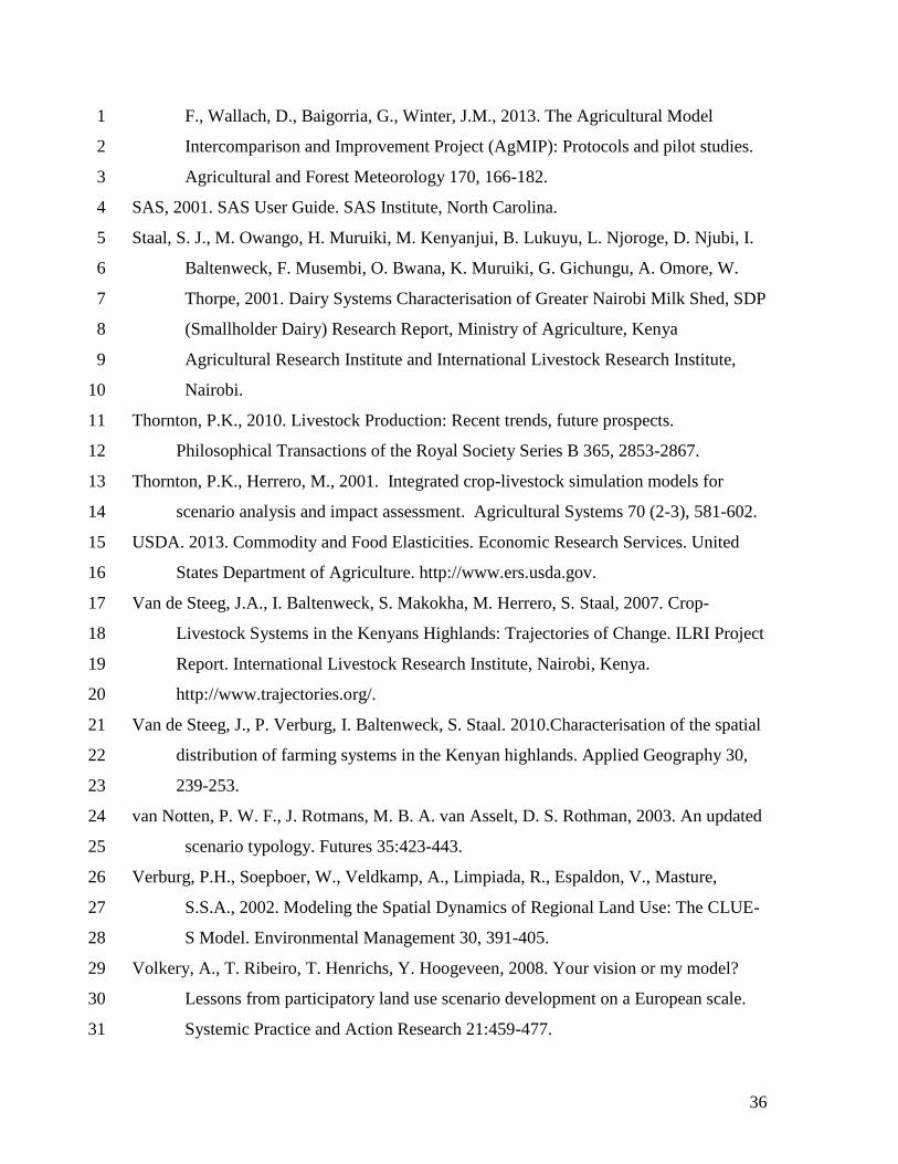
36

F., Wallach, D., Baigorria, G., Winter, J.M., 2013. The Agricultural Model 1

Intercomparison and Improvement Project (AgMIP): Protocols and pilot studies. 2

Agricultural and Forest Meteorology 170, 166-182. 3

SAS, 2001. SAS User Guide. SAS Institute, North Carolina. 4

Staal, S. J., M. Owango, H. Muruiki, M. Kenyanjui, B. Lukuyu, L. Njoroge, D. Njubi, I. 5

Baltenweck, F. Musembi, O. Bwana, K. Muruiki, G. Gichungu, A. Omore, W. 6

Thorpe, 2001. Dairy Systems Characterisation of Greater Nairobi Milk Shed, SDP 7

(Smallholder Dairy) Research Report, Ministry of Agriculture, Kenya 8

Agricultural Research Institute and International Livestock Research Institute, 9

Nairobi. 10

Thornton, P.K., 2010. Livestock Production: Recent trends, future prospects. 11

Philosophical Transactions of the Royal Society Series B 365, 2853-2867. 12

Thornton, P.K., Herrero, M., 2001. Integrated crop-livestock simulation models for 13

scenario analysis and impact assessment. Agricultural Systems 70 (2-3), 581-602. 14

USDA. 2013. Commodity and Food Elasticities. Economic Research Services. United 15

States Department of Agriculture. http://www.ers.usda.gov. 16

Van de Steeg, J.A., I. Baltenweck, S. Makokha, M. Herrero, S. Staal, 2007. Crop-17

Livestock Systems in the Kenyans Highlands: Trajectories of Change. ILRI Project 18

Report. International Livestock Research Institute, Nairobi, Kenya. 19

http://www.trajectories.org/. 20

Van de Steeg, J., P. Verburg, I. Baltenweck, S. Staal. 2010.Characterisation of the spatial 21

distribution of farming systems in the Kenyan highlands. Applied Geography 30, 22

239-253. 23

van Notten, P. W. F., J. Rotmans, M. B. A. van Asselt, D. S. Rothman, 2003. An updated 24

scenario typology. Futures 35:423-443. 25

Verburg, P.H., Soepboer, W., Veldkamp, A., Limpiada, R., Espaldon, V., Masture, 26

S.S.A., 2002. Modeling the Spatial Dynamics of Regional Land Use: The CLUE-27

S Model. Environmental Management 30, 391-405. 28

Volkery, A., T. Ribeiro, T. Henrichs, Y. Hoogeveen, 2008. Your vision or my model? 29

Lessons from participatory land use scenario development on a European scale. 30

Systemic Practice and Action Research 21:459-477. 31

37

Waithaka, M., A. Wokabi, J. Nyangaga, E. Ouma, J. Biwott, S. Staal, M. Ojowi, R. 1

Ogidi, I. Njarro, P. Mudavadi, 2000. A participatory rapid appraisal (PRA) of 2

farming systems in western Kenya. In: Proceedings of the Report of a PRA on 3

Dairy and Crop Activities in Western Kenya, 24 January to 5 February, 2000. 4

MoA/KARI/ILRI Smallholder Dairy (Research & Development) Project Report. 5

Waithaka, M.M., Thornton, P.K., Shepherd, K.D., Herrero, M., 2006. Bio-economic 6

evaluation of farmers’ perceptions of sustainable farms in Western Kenya. 7

Agricultural Systems 90, 243-271. 8

Wiggins, S., 2009 Can the smallholder model deliver poverty reduction and food security 9

for a rapidly growing population in Africa? Background paper for the Expert 10

Meeting on How to feed the World in 2050, Food and Agriculture Organization of 11

the United Nations. Online at www.fao.org/docrep/012/ak542e/ak542e00.htm. 12

Wilkinson, A., Eidinow, E., 2008. Evolving practices in environmental scenarios: A new 13

scenario typology. Environmental Research Letters 3:045017. 14

World Bank, 2009. Minding the stock: bringing public policy to bear on livestock sector 15

development. Report no. 44010-GLB.Washington, DC. 16

Xiang, W. N., Clarke, K.C., 2003. The use of scenarios in land-use planning. 17

Environment and Planning B: Planning and Design 30:885-909. 18

Zingore, S., Gonzalez-Estrada, E., Delve, R.J., Herrero, M., Dimes, J., Giller, K., 2009. 19

An integrated evaluation of strategies for enhancing productivity and profitability 20

of resource-constrained smallholder farms in Zimbabwe. Agricultural Systems 21

101, 57–68. 22

Zurek, M. B., Henrichs, T., 2007. Linking scenarios across geographical scales in 23

international environmental assessments. Technological Forecasting and Social 24

Change 74:1282-1295. 25

26

27

28

38

Figures 1

2

Figure 1: Map of the study area 3

4

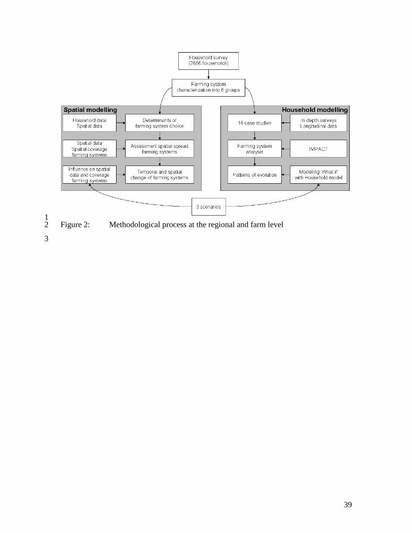
39

1 Figure 2: Methodological process at the regional and farm level 2

3

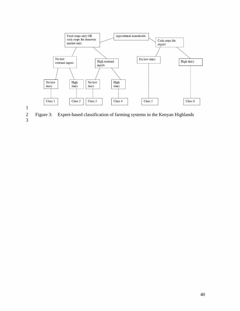
40

1

Figure 3: Expert-based classification of farming systems in the Kenyan Highlands 2

3

41

1 2

Figure 4: Projections of land size and labour price for the three case studies and 3

scenarios (2005-2025) which serve as inputs for the Household Model 4

analyses 5

6

Baseline Case study 1 Baseline Case study 2 Baseline Case study 3

Equitable Case study 1 Equitable Case study 2 Equitable Case study 3

Inequitable Case study 1 Inequitable Case study 2 Inequitable Case study 3

Baseline Case study 1 Baseline Case study 2 Baseline Case study 3

Equitable Case study 1 Equitable Case study 2 Equitable Case study 3

Inequitable Case study 1 Inequitable Case study 2 Inequitable Case study 3

0

1

2

3

4

5

6

7

2005 2010 2015 2020 2025

year

ha

0.150

0.170

0.190

0.210

0.230

0.250

0.270

0.290

0.310

2005 2010 2015 2020 2025

year

€/ h

42

1 Figure 5: Predicted spatial distribution of farming systems for the year 2005, and spatial 2

and aggregated change in farming systems for different scenarios in 2025 (the 3

grey areas represent areas without change). 4

5

43

Figure 6: Case Study 1: evolution of subsistence farm with dairy; signs above the bar 1

show the trend in the five-year period of simulation (increase, decrease, equal); white 2

bars in milk orientation graph are non-milking cattle 3

4

5 6

0

0.005

0.01

0.015

0.02

0.025

0.03

0.035

are

a [h

a]

Food Crops - Maize

0

0.5

1

1.5

2

2.5

are

a [h

a]

Food / Cash Crops - Maize-Beans

Observed

Optimal base

2005 - 2010

2020 - 2025

0

0.1

0.2

0.3

0.4

0.5

0.6

0.7

0.8

0.9

are

a [h

a]

Cash Crops - Passion

0

0.02

0.04

0.06

0.08

0.1

0.12

0.14

0.16

0.18

0.2

are

a [h

a]

Grassland

0

0.5

1

1.5

2

2.5

are

a [h

a]

Cut and Carry

0

2

4

6

8

10

12

Nr

of

Co

ws,

wh

ite

of

wh

ich

are

milk

ing

Milk orientation

0

500

1000

1500

2000

2500

Ho

urs

of

lab

ou

r

Hired Labour

T1 T2 T1 T2Baseline Equitable

T1 T2 T1 T2Baseline Equitable

T1 T2 T1 T2Baseline Equitable

T1 T2 T1 T2Baseline Equitable

InequitableT1 T2

InequitableT1 T2

InequitableT1 T2

T1 T2 T1 T2Baseline Equitable Inequitable

T1 T2 T1 T2 T1 T2Baseline Equitable Inequitable

T1 T2

T1 T2 T1 T2Baseline Equitable Inequitable

T1 T2

InequitableT1 T2

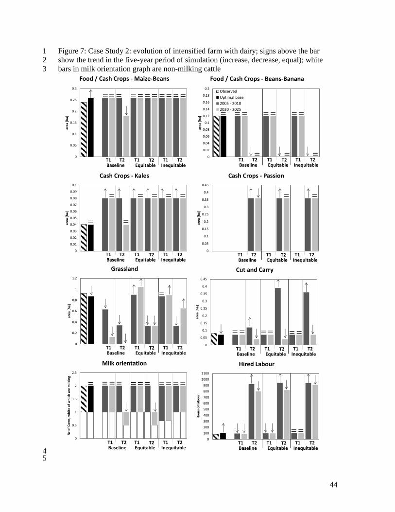
44

Figure 7: Case Study 2: evolution of intensified farm with dairy; signs above the bar 1

show the trend in the five-year period of simulation (increase, decrease, equal); white 2

bars in milk orientation graph are non-milking cattle 3

4 5

0

0.05

0.1

0.15

0.2

0.25

0.3

are

a [h

a]

Food / Cash Crops - Maize-Beans

0

0.02

0.04

0.06

0.08

0.1

0.12

0.14

0.16

0.18

0.2

are

a [h

a]

Food / Cash Crops - Beans-Banana

Observed

Optimal base

2005 - 2010

2020 - 2025

0

0.01

0.02

0.03

0.04

0.05

0.06

0.07

0.08

0.09

0.1

are

a [h

a]

Cash Crops - Kales

0

0.2

0.4

0.6

0.8

1

1.2

are

a [h

a]

Grassland

0

0.05

0.1

0.15

0.2

0.25

0.3

0.35

0.4

0.45

are

a [h

a]

Cut and Carry

0

0.5

1

1.5

2

2.5

Nr

of

Co

ws,

wh

ite

of

wh

ich

are

milk

ing

Milk orientation

0

100

200

300

400

500

600

700

800

900

1000

1100

Ho

urs

of

lab

ou

r

Hired Labour

0

0.05

0.1

0.15

0.2

0.25

0.3

0.35

0.4

0.45

are

a [h

a]

Cash Crops - Passion

T1 T2 T1 T2Baseline Equitable Inequitable

T1 T2 T1 T2 T1 T2Baseline Equitable Inequitable

T1 T2

T1 T2 T1 T2Baseline Equitable Inequitable

T1 T2 T1 T2 T1 T2Baseline Equitable Inequitable

T1 T2

T1 T2 T1 T2Baseline Equitable Inequitable

T1 T2 T1 T2 T1 T2Baseline Equitable Inequitable

T1 T2

T1 T2 T1 T2Baseline Equitable Inequitable

T1 T2 T1 T2 T1 T2Baseline Equitable Inequitable

T1 T2

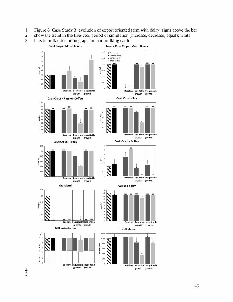
45

Figure 8: Case Study 3: evolution of export oriented farm with dairy; signs above the bar 1

show the trend in the five-year period of simulation (increase, decrease, equal); white 2

bars in milk orientation graph are non-milking cattle 3

4 5

0

0.2

0.4

0.6

0.8

1

1.2

1.4

1.6

are

a [h

a]

Food Crops - Maize-Beans

0

0.05

0.1

0.15

0.2

0.25

0.3

are

a [h

a]

Food / Cash Crops - Maize-Beans

ObservedOptimal base2005 - 20102020 - 2025

0

0.1

0.2

0.3

0.4

0.5

0.6

0.7

0.8

0.9

are

a [h

a]

Cash Crops - Passion-Coffee

0

0.05

0.1

0.15

0.2

0.25

are

a [h

a]

Grassland

0

0.1

0.2

0.3

0.4

0.5

0.6

0.7

0.8

0.9

1

are

a [h

a]

Cut and Carry

0

2

4

6

8

10

12

Nr

of

Co

ws,

wh

ite

of

wh

ich

are

milk

ing

Milk orientation

0

200

400

600

800

1000

1200

Ho

urs

of

lab

ou

r

Hired Labour

0

0.2

0.4

0.6

0.8

1

1.2ar

ea

[ha]

Cash Crops - Tea

0

0.02

0.04

0.06

0.08

0.1

0.12

are

a [h

a]

Cash Crops - Trees

0

0.5

1

1.5

2

2.5

3

3.5

are

a [h

a]

Cash Crops - Coffee

Baseline Equitablegrowth

Inequitablegrowth

Baseline Equitablegrowth

Inequitablegrowth

Baseline Equitablegrowth

Inequitablegrowth

Baseline Equitablegrowth

Inequitablegrowth

Baseline Equitablegrowth

Inequitablegrowth

Baseline Equitablegrowth

Inequitablegrowth

Baseline Equitablegrowth

Inequitablegrowth

Baseline Equitablegrowth

Inequitablegrowth

Baseline Equitablegrowth

Inequitablegrowth

Baseline Equitablegrowth

Inequitablegrowth

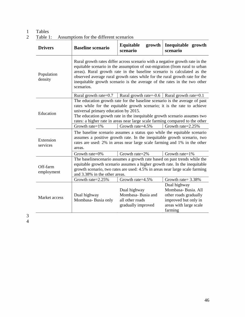
46

Tables 1

Table 1: Assumptions for the different scenarios 2

Drivers Baseline scenario Equitable growth

scenario

Inequitable growth

scenario

Population

density

Rural growth rates differ across scenario with a negative growth rate in the

equitable scenario in the assumption of out-migration (from rural to urban

areas). Rural growth rate in the baseline scenario is calculated as the

observed average rural growth rates while for the rural growth rate for the

inequitable growth scenario is the average of the rates in the two other

scenarios.

Rural growth rate=0.7 Rural growth rate=-0.6 Rural growth rate=0.1

Education

The education growth rate for the baseline scenario is the average of past

rates while for the equitable growth scenario; it is the rate to achieve

universal primary education by 2015.

The education growth rate in the inequitable growth scenario assumes two

rates: a higher rate in areas near large scale farming compared to the other

areas. Growth rate=1% Growth rate=4.5% Growth rate=2.25%

Extension

services

The baseline scenario assumes a status quo while the equitable scenario

assumes a positive growth rate. In the inequitable growth scenario, two

rates are used: 2% in areas near large scale farming and 1% in the other

areas.

Growth rate=0% Growth rate=2% Growth rate=1%

Off-farm

employment

The baselinescenario assumes a growth rate based on past trends while the

equitable growth scenario assumes a higher growth rate. In the inequitable

growth scenario, two rates are used: 4.5% in areas near large scale farming

and 3.38% in the other areas.

Growth rate=2.25% Growth rate=4.5% Growth rate= 3.38%

Market access Dual highway

Mombasa- Busia only

Dual highway

Mombasa- Busia and

all other roads

gradually improved

Dual highway

Mombasa- Busia. All

other roads gradually

improved but only in

areas with large scale

farming

3

4

47

Table 2: Main characteristics of case study households, 2005 1

Variable

subsistence farm with

dairy

intensified farm with

dairy

export oriented farm

with dairy

General Characteristics

Location (elevation,

m.a.s.l.)

Vihiga (1542) Nandi (2131) Kiambu (1954)

Family size (working) 8 (5) 7 (4) 6 (4)

Farm size, ha (no. of

plots)

2.46 (6) 1.40 (7) 4.8 (7)

% of crops 17.5% 71.4% 77.1%

Main crops maize, beans maize, beans, kales tea, coffee, passion

fruit, beans, maize,

potato

Livestock numbers Cattle (milking): 8

(4)

Goats: 10, Chicken:

20

Cattle (milking): 2

(1)

Sheep: 3, Chicken: 10

Cattle (milking): 10

(5)

Sheep: 3, Chicken: 13

Economics: income and expenditure

Annual incomes

agriculture

livestock

off-farm Annual expenditure

agriculture

livestock

other expenses Net annual income from

agricultural activities, €

1610.2 846.2 3083.7

Contribution of off-farm

income to total income, %

20.8% 18.8% 0%

Agric. products with

highest contribution to

income

milk, maize kales, milk milk, passion fruit,

tea, coffee

Annual agricultural

income per person, €

322.4 184.9 1077.3

Annual agricultural

income per ha, €

1397.9 1233.0 1795.5

Sources of annual food security (energy and protein)

Energy sources

On-farm agric.

prod.

on-farm livest.

prod.

purchased products

48

Protein sources

on-farm agric.

prod.

on-farm livest.

prod.

purchased products

Family’s energy

requirements met

(deficit)

NO (11.6%) NO (1.3%) YES

Family’s protein

requirements met

YES YES YES

Proportion of income

spent in purchasing food

11.8% 14.2% 6.8%

On-farm prod. with

highest contribution to

family’s nutrition

maize, milk maize, milk, beans maize, milk

1

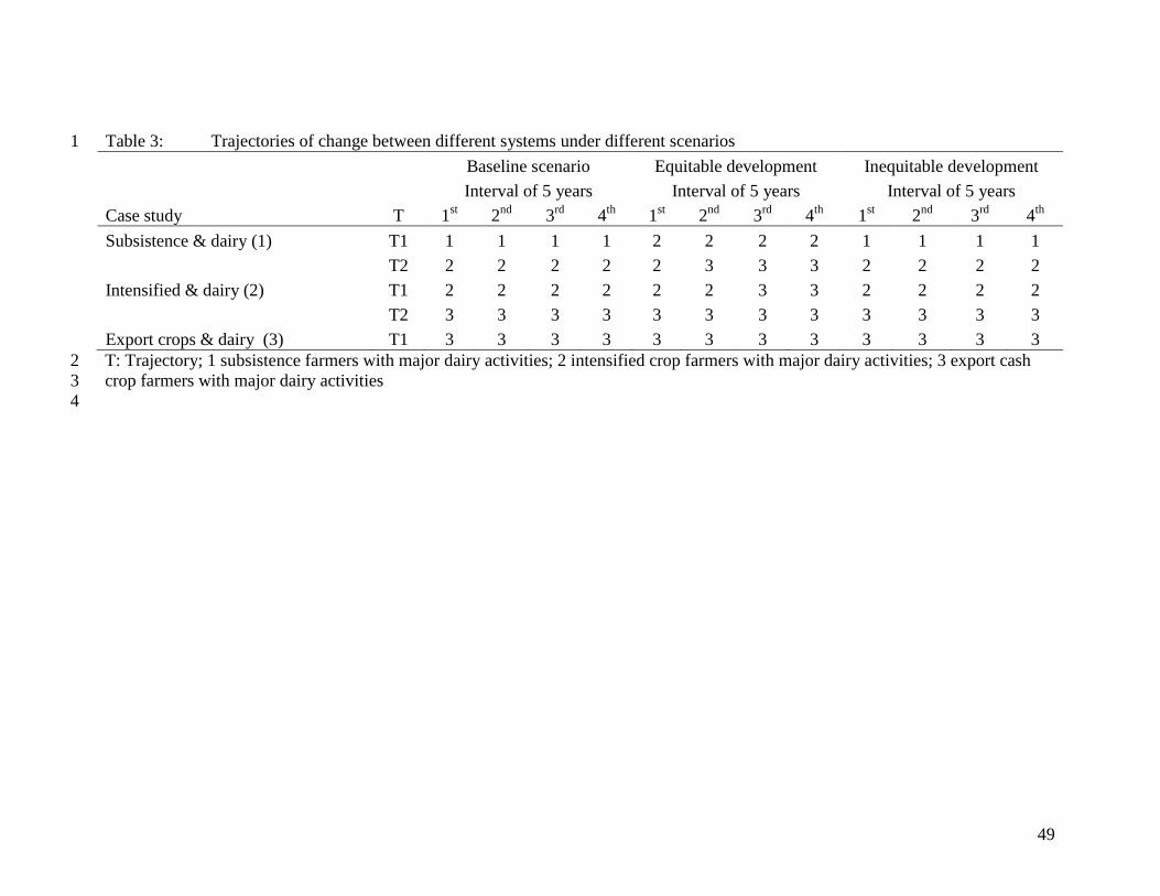
49

Table 3: Trajectories of change between different systems under different scenarios 1

Baseline scenario Equitable development Inequitable development

Interval of 5 years Interval of 5 years Interval of 5 years

Case study T 1st 2

nd 3

rd 4

th 1

st 2

nd 3

rd 4

th 1

st 2

nd 3

rd 4

th

Subsistence & dairy (1) T1 1 1 1 1 2 2 2 2 1 1 1 1

T2 2 2 2 2 2 3 3 3 2 2 2 2

Intensified & dairy (2) T1 2 2 2 2 2 2 3 3 2 2 2 2

T2 3 3 3 3 3 3 3 3 3 3 3 3

Export crops & dairy (3) T1 3 3 3 3 3 3 3 3 3 3 3 3

T: Trajectory; 1 subsistence farmers with major dairy activities; 2 intensified crop farmers with major dairy activities; 3 export cash 2

crop farmers with major dairy activities 3

4

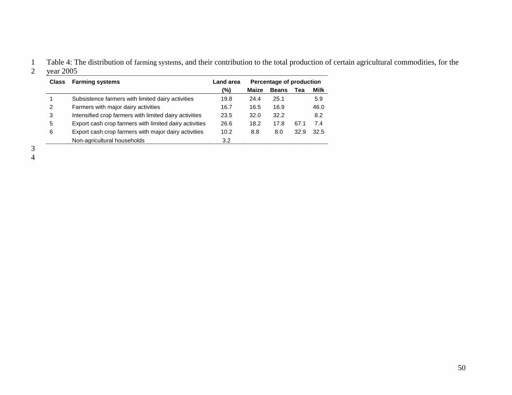
50

Table 4: The distribution of farming systems, and their contribution to the total production of certain agricultural commodities, for the 1

year 2005 2

Class Farming systems Land area Percentage of production

(%) Maize Beans Tea Milk

1 Subsistence farmers with limited dairy activities 19.8 24.4 25.1

5.9

2 Farmers with major dairy activities 16.7 16.5 16.9

46.0

3 Intensified crop farmers with limited dairy activities 23.5 32.0 32.2

8.2

5 Export cash crop farmers with limited dairy activities 26.6 18.2 17.8 67.1 7.4

6 Export cash crop farmers with major dairy activities 10.2 8.8 8.0 32.9 32.5

Non-agricultural households 3.2

3

4

51

Table 5: Demand for commodities (tons/year/person) 1

Baseline scenario Equitable growth scenario Inequitable growth scenario

Maize Beans Milk Tea Maize Beans Milk Tea Maize Beans Milk Tea

2004 0.103 0.007 0.087 0.777 0.103 0.007 0.087 0.777 0.103 0.007 0.087 0.777

2005 0.103 0.007 0.088 0.786 0.106 0.008 0.091 0.837 0.105 0.008 0.089 0.811

2006 0.104 0.007 0.088 0.795 0.109 0.008 0.095 0.900 0.106 0.008 0.091 0.847

2007 0.104 0.008 0.089 0.804 0.112 0.008 0.099 0.969 0.108 0.008 0.094 0.884

2008 0.105 0.008 0.089 0.813 0.115 0.009 0.103 1.042 0.110 0.008 0.096 0.922

2009 0.105 0.008 0.090 0.822 0.118 0.009 0.107 1.122 0.111 0.008 0.098 0.963

2010 0.105 0.008 0.090 0.832 0.121 0.009 0.112 1.207 0.113 0.008 0.101 1.005

2011 0.106 0.008 0.091 0.841 0.124 0.010 0.117 1.299 0.115 0.009 0.103 1.049

2012 0.106 0.008 0.092 0.851 0.128 0.010 0.122 1.397 0.117 0.009 0.106 1.094

2013 0.107 0.008 0.092 0.860 0.131 0.010 0.127 1.504 0.118 0.009 0.108 1.142

2014 0.107 0.008 0.093 0.870 0.135 0.011 0.132 1.618 0.120 0.009 0.111 1.192

2015 0.108 0.008 0.093 0.880 0.139 0.011 0.138 1.741 0.122 0.009 0.114 1.244

2016 0.108 0.008 0.094 0.890 0.142 0.012 0.144 1.873 0.124 0.010 0.116 1.299

2017 0.108 0.008 0.095 0.900 0.146 0.012 0.150 2.016 0.126 0.010 0.119 1.355

2018 0.109 0.008 0.095 0.910 0.150 0.012 0.156 2.169 0.128 0.010 0.122 1.415

2019 0.109 0.008 0.096 0.920 0.154 0.013 0.163 2.334 0.130 0.010 0.125 1.476

2020 0.110 0.008 0.096 0.931 0.159 0.013 0.170 2.512 0.132 0.010 0.128 1.541

2021 0.110 0.008 0.097 0.941 0.163 0.014 0.177 2.703 0.134 0.011 0.131 1.608

2022 0.111 0.008 0.098 0.952 0.167 0.014 0.185 2.908 0.136 0.011 0.135 1.678

2023 0.111 0.008 0.098 0.963 0.172 0.015 0.192 3.129 0.138 0.011 0.138 1.752

2024 0.112 0.008 0.099 0.974 0.177 0.016 0.201 3.367 0.141 0.011 0.141 1.828

2

3

52

Table 6: The distribution of farming systems over 20 years, driven by the combined changes in the demand for different commodities 1

Farming System Scenario Land area (%)

2005 2010 2015 2020 2025

Subsistence farmers with limited dairy activities

Baseline 19.76 19.64 19.51 19.38 19.26

Equitable growth 19.75 19.59 19.42 19.24 19.08

Inequitable growth 19.76 19.63 19.50 19.36 19.25

Farmers with major dairy activities

Baseline 16.70 16.65 16.60 16.54 16.49

Equitable growth 16.70 16.63 16.56 16.49 16.44

Inequitable growth 16.70 16.65 16.60 16.54 16.51

Intensified crop farmers with limited dairy activities

Baseline 23.44 23.31 23.17 23.01 22.88

Equitable growth 23.43 23.25 23.06 22.85 22.68

Inequitable growth 23.44 23.29 23.15 22.99 22.87

Export cash crop farmers with limited dairy activities

Baseline 26.58 26.50 26.41 26.30 26.22

Equitable growth 26.60 26.58 26.55 26.51 26.48

Inequitable growth 26.60 26.56 26.51 26.46 26.43

Export cash crop farmers with major dairy activities

Baseline 10.25 10.28 10.31 10.34 10.37

Equitable growth 10.26 10.34 10.43 10.52 10.61

Inequitable growth 10.25 10.31 10.36 10.43 10.49

Non-agricultural households

Baseline 3.28 3.62 4.01 4.42 4.79

Equitable growth 3.27 3.61 3.98 4.38 4.72

Inequitable growth 3.28 3.62 4.01 4.42 4.79

2

3

53

Table 7: Overview of spatial changes in farming system over 20 years, under different scenarios 1

Farming system for various years Surface area changes (%)

by growth scenario

2005 2025 Baseline Equitable Inequitable

Subsistence farmers with limited dairy

Subsistence farmers with limited dairy 0 0 0

Farmers with major dairy activities 1.2 1.2 1.2

Intensified crop farmers with limited dairy 5.3 5.4 5.8

Export cash crop farmers with limited dairy 15.9 21.0 20.6

Export cash crop farmers with major dairy 0 0 0

Non-agricultural households 0.4 0 0

Farmers with major dairy activities

Subsistence farmers with limited dairy 0 0 0

Farmers with major dairy activities 0 0 0

Intensified crop farmers with limited dairy 0.2 0.5 0.3

Export cash crop farmers with limited dairy 2.2 3.1 3.1

Export cash crop farmers with major dairy 3.4 4.1 4.1

Non-agricultural households 0 0 0

Intensified crop farmers with limited dairy

Subsistence farmers with limited dairy 0.1 0.1 0.2

Farmers with major dairy activities 5.9 3.4 3.3

Intensified crop farmers with limited dairy 0.0 0 0

Export cash crop farmers with limited dairy 16.2 16.9 17.1

Export cash crop farmers with major dairy 11.7 15.7 15.8

Non-agricultural households 0 0.0 0.0

Export cash crop farmers with limited dairy

Subsistence farmers with limited dairy 0 0.0 0.0

Farmers with major dairy activities 2.1 1.1 1.0

Intensified crop farmers with limited dairy 4.7 0.5 0.5

Export cash crop farmers with limited dairy 0 0 0

Export cash crop farmers with major dairy 21.5 18.8 18.7

Non-agricultural households 0 0.0 0

Export cash crop farmers with major dairy

Subsistence farmers with limited dairy 0 0 0

Farmers with major dairy activities 0.9 0.1 0.1

Intensified crop farmers with limited dairy 0.3 0.0 0.1

Export cash crop farmers with limited dairy 0.0 0 0

Export cash crop farmers with major dairy 0 0 0

54

Non-agricultural households 0 0 0

Non-agricultural households

Subsistence farmers with limited dairy 0.1 0.0 0

Farmers with major dairy activities 2.7 1.9 1.8

Intensified crop farmers with limited dairy 1.4 0.7 0.8

Export cash crop farmers with limited dairy 3.4 4.6 4.5

Export cash crop farmers with major dairy 0.5 0.8 0.8

Non-agricultural households 0 0 0

1

2