EVEN SEM 2017 - SRM Institute of Science and · PDF filearockia vijay joseph |ei1106- mcs|23.01.2017 even sem 2017 arockia vijay joseph department of eie, srm university even sem 2017

AROCKIA VIJAY JOSEPH |EI1106- MCS|23.01.2017

EVEN

SEM

2017

AROCKIA VIJAY JOSEPH

DEPARTMENT OF EIE, SRM

UNIVERSITY

EVEN SEM 2017

MODERN CONTROL SYSTEMS


MODERN CONTROL SYSTEMS

Total Contact Hours – 45

Prerequisite CONTROL SYSTEMS ENGINEERING

PURPOSE To gain knowledge in compensator and controller design, state variable analysis, non-linear systems

and optimal control.

INSTRUCTIONAL OBJECTIVES 1. To design cascade compensators in time domain and design PID controllers in time domain

and frequency domain.

2. To understand and develop state space model for different systems.

3. To analyse the controllability and observability of a system and to design controllers and

observers.

4. To give a basic knowledge in non-linearity and methods to find the stability of non-linear

systems.

5. To understand the need of optimality and solving problems.

UNIT – I LINEAR CONTROL DESIGN (9 hours) Design specifications- compensator configuration (series and feedback)-design cascade and feedback

compensators (lag, lead, lag-lead) by using time domain. Introduction of PID controllers and design

PD, PI, PID controllers using time and frequency domain methods

UNIT – II STATE SPACE ANALYSIS (9 hours) Concepts of State, State variable and State space model- State space representation of linear

continuous time systems using physical variables, phase variables and canonical variables-

diagonalization-State space representation of discrete time systems-Solution of state equations-

computation of state transition matrix.

UNIT III - CONTROLLABILITY AND OBSERVABILITY (9 hours)

BIBO Stability – Determining the stability by Routh-Hurwitz criterion- Properties and construction of

the root loci-effect of adding a pole and zeros to a system

UNIT IV – NON-LINEAR CONTROL (9 hours) Non-linear systems-properties-common physical non-linearity’s-dead zone, relay, saturation

nonlinearities phase plane method-singular points-phase trajectories- stability analysis by describing

function method-Liapunov's stability criterion.

UNIT – V OPTIMAL CONTROL (9 hours) Problem formulation – necessary conditions of optimality – state regulator problem – Matrix Riccati

equation – infinite time regulator problem – output regulator and tracking problems

TEXT BOOKS 1. Gopal. M, “Modern Control System theory”, New age international(P) ltd, 2012. 2. Nagrath.I.J, and Gopal .M, “Control Systems Engineering”, Anshan Pub, 2008.

REFERENCES

1. Katsuhiko Ogata, “Modern Control Engineering”-fifth edition, Prentice Hall of India Private Ltd,

New Delhi, 2009.

2. Kirk D.E, “Optimal control theory-an introduction”, Prentice Hall, N.J. 1970. 3. Richard .C, Dorf and Robert.H.Bishop, “Modern Control System Engineering”, Pearson Education (US), United States, 2010.


UNIT I - LINEAR CONTROL DESIGN

COMPENSATORS

1.1 Lead Compensation Techniques Based on the Root-Locus Approach

The root-locus approach to design is very powerful when the specifications are given in terms of

time-domain quantities, such as the damping ratio and undamped natural frequency of the desired

dominant closed-loop poles, maximum overshoot, rise time, and settling time. Consider a design

problem in which the original system either is unstable for all values of gain or is stable but has

undesirable transient-response characteristics. In such a case, the reshaping of the root locus is

necessary in the broad neighbourhood of the jω axis and the origin in order that the dominant

closed-loop poles be at desired locations in the complex plane. This problem may be solved by

inserting an appropriate lead compensator in cascade with the feed forward transfer function.

The procedures for designing a lead compensator for the system shown in Figure by the root-

locus method may be stated as follows:

1. From the performance specifications, determine the desired location for the dominant closed-

loop poles.

2. By drawing the root-locus plot of the uncompensated system (original system), ascertain

whether or not the gain adjustment alone can yield the desired closed- loop poles. If not, calculate

the angle deficiency φ. This angle must be contributed by the lead compensator if the new root

locus is to pass through the desired locations for the dominant closed-loop poles.

3. Assume the lead compensator (s) to be

1

where α and T are determined from the angle deficiency. is determined from the requirement

of the open-loop gain.

4. If static error constants are not specified, determine the location of the pole and zero of the

lead compensator so that the lead compensator will contribute the necessary angle φ. If no other

requirements are imposed on the system, try to make the value of α as large as possible. A larger

value of α generally results in a larger value of 𝑣, which is desirable. (If a particular static error

constant is specified, it is generally simpler to use the frequency-response approach.)

5. Determine the open-loop gain of the compensated system from the magnitude condition.

Once a compensator has been designed, check to see whether all performance specifications have

been met. If the compensated system does not meet the performance specifications, then repeat

the design procedure by adjusting the compensator pole and zero until all such specifications are

met. If a large static error constant is required, cascade a lag network or alter the lead

compensator to a lag-lead compensator.

Note that if the selected dominant closed-loop poles are not really dominant, it will be necessary

to modify the location of the pair of such selected dominant closed-loop poles. (The closed-loop

poles other than dominant ones modify the response obtained from the dominant closed-loop


poles alone. The amount of modification depends on the location of these remaining closed-loop

poles.) Also, the closed-loop zeros affect the response if they are located near the origin.

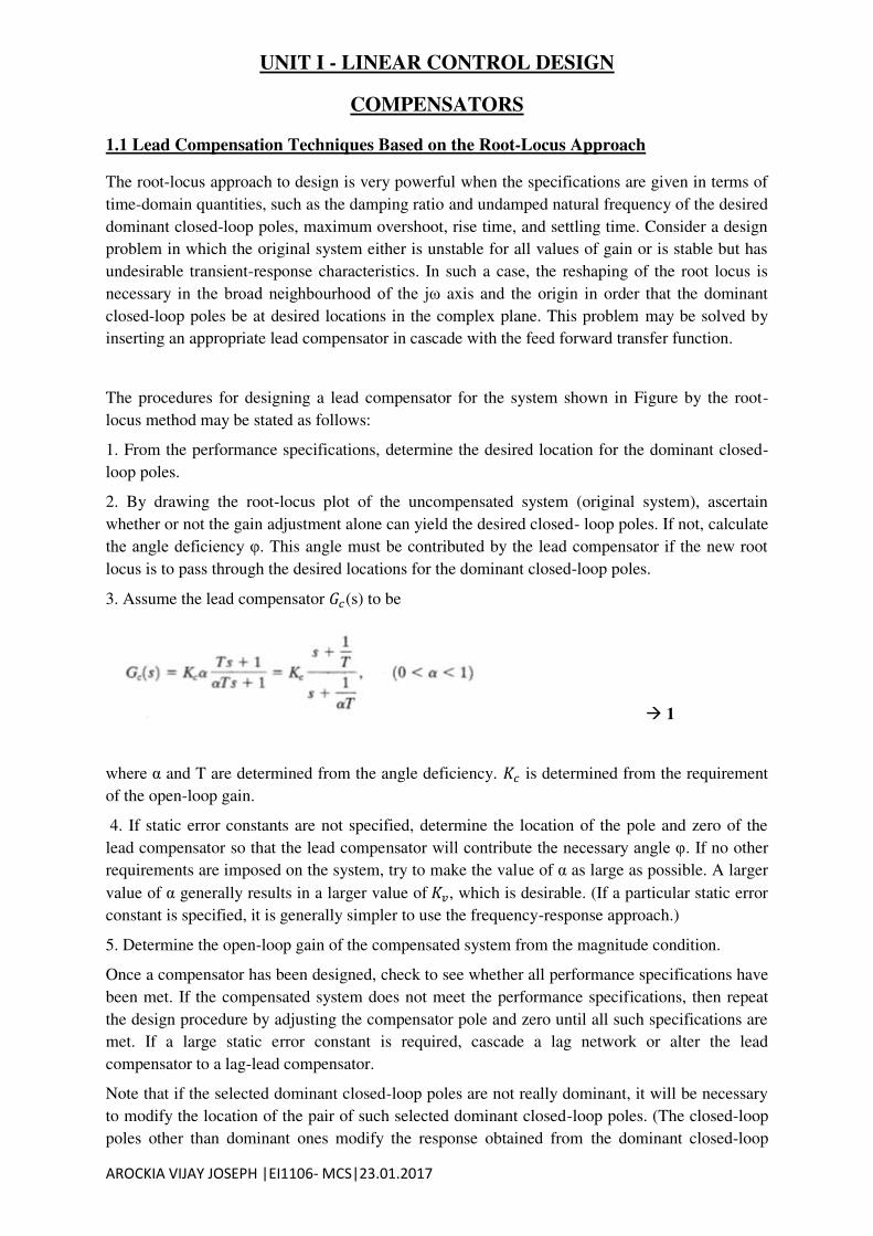
Example 1: Consider the block diagram of a model for an attitude-rate control system.

It is desired to speed up the response and also eliminate the oscillatory mode at the beginning of

the response. Design a suitable lead compensator such that the dominant closed-loop poles are at

s = -2 ± j2√3.




1.2 Lag Compensation Techniques Based on the Root-Locus Approach

Consider the problem of finding a suitable compensation network for the case where the system

exhibits satisfactory transient-response characteristics but unsatisfactory steady-state

characteristics. Compensation in this case essentially consists of increasing the open- loop gain

without appreciably changing the transient-response characteristics. This means that the root

locus in the neighbourhood of the dominant closed-loop poles should not be changed appreciably,

but the open-loop gain should be increased as much as needed. This can be accomplished if a lag

compensator is put in cascade with the given feed forward transfer function. To avoid an

appreciable change in the root loci, the angle contribution of the lag network should be limited

to a small amount, say 5 .To assure this, we place the pole and zero of the lag network relatively

close together and near the origin of the s plane. Then the closed-loop poles of the compensated

system will be shifted only slightly from their original locations. Hence, the transient-response

characteristics will be changed only slightly. Consider a lag compensator G(s), where

2

If we place the zero and pole of the lag compensator very close to each other, then at s = ,

where , is one of the dominant closed-loop poles, the magnitudes + (1/T) and + [1/( T)] are

almost equal, or

3

To make the angle contribution of the lag portion of the compensator to be small, we require

4

This implies that if gain , of the lag compensator is set equal to 1, then the transient- response

characteristics will not be altered. (This means that the overall gain of the open-loop transfer

function can be increased by a factor of where > 1.) If the pole and zero are placed very close

to the origin, then the value of can be made large. (A large value of may be used, provided

physical realization of the lag compensator is possible.) It is noted that the value of T must be

large, but its exact value is not critical. However, it should not be too large in order to avoid

difficulties in realizing the phase lag compensator by physical components.

An increase in the gain means an increase in the static error constants. If the open-loop transfer

function of the uncompensated system is G(s), then the static velocity error constant 𝑣, of the

uncompensated system is

5


If the compensator is chosen as given by Equation (2), then for the compensated system with the

open-loop transfer function (s)G(s) the static velocity error constant ��, becomes

6

Thus if the compensator is given by Equation (2), then the static velocity error constant is

increased by a factor of , where is approximately unity.

The main negative effect of the lag compensation is that the compensator zero that will be

generated near the origin creates a closed-loop pole near the origin. This closed- loop pole and

compensator zero will generate a long tail of small amplitude in the step response, thus increasing

the settling time.

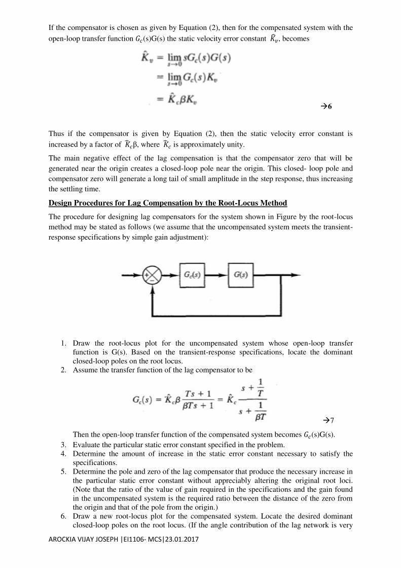
Design Procedures for Lag Compensation by the Root-Locus Method

The procedure for designing lag compensators for the system shown in Figure by the root-locus

method may be stated as follows (we assume that the uncompensated system meets the transient-

response specifications by simple gain adjustment):

1. Draw the root-locus plot for the uncompensated system whose open-loop transfer

function is G(s). Based on the transient-response specifications, locate the dominant

closed-loop poles on the root locus.

2. Assume the transfer function of the lag compensator to be

7

Then the open-loop transfer function of the compensated system becomes (s)G(s).

3. Evaluate the particular static error constant specified in the problem.

4. Determine the amount of increase in the static error constant necessary to satisfy the

specifications.

5. Determine the pole and zero of the lag compensator that produce the necessary increase in

the particular static error constant without appreciably altering the original root loci.

(Note that the ratio of the value of gain required in the specifications and the gain found

in the uncompensated system is the required ratio between the distance of the zero from

the origin and that of the pole from the origin.)

6. Draw a new root-locus plot for the compensated system. Locate the desired dominant

closed-loop poles on the root locus. (If the angle contribution of the lag network is very


small, that is, a few degrees, then the original and new root loci are almost identical.

Otherwise, there will be a slight discrepancy between them. Then locate, on the new root

locus, the desired dominant closed-loop poles based on the transient-response

specifications.)

7. Adjust gain of the compensator from the magnitude condition so that the dominant

closed-loop poles lie at the desired location. ( Will be approximately 1.)

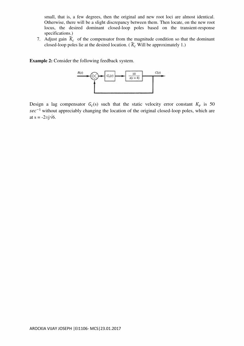
Example 2: Consider the following feedback system.

Design a lag compensator (s) such that the static velocity error constant 𝑣 is 50 − without appreciably changing the location of the original closed-loop poles, which are

at s = -2±j√6.




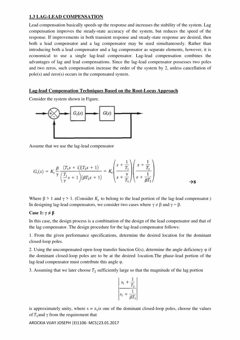
1.3 LAG-LEAD COMPENSATION

Lead compensation basically speeds up the response and increases the stability of the system. Lag

compensation improves the steady-state accuracy of the system, but reduces the speed of the

response. If improvements in both transient response and steady-state response are desired, then

both a lead compensator and a lag compensator may be used simultaneously. Rather than

introducing both a lead compensator and a lag compensator as separate elements, however, it is

economical to use a single lag-lead compensator. Lag-lead compensation combines the

advantages of lag and lead compensations. Since the lag-lead compensator possesses two poles

and two zeros, such compensation increase the order of the system by 2, unless cancellation of

pole(s) and zero(s) occurs in the compensated system.

Lag-lead Compensation Techniques Based on the Root-Locus Approach

Consider the system shown in Figure.

Assume that we use the lag-lead compensator

8

Where > 1 and > 1. (Consider to belong to the lead portion of the lag-lead compensator.)

In designing lag-lead compensators, we consider two cases where ≠ and = .

Case 1: ≠

In this case, the design process is a combination of the design of the lead compensator and that of

the lag compensator. The design procedure for the lag-lead compensator follows:

1. From the given performance specifications, determine the desired location for the dominant

closed-loop poles.

2. Using the uncompensated open-loop transfer function G(s), determine the angle deficiency φ if

the dominant closed-loop poles are to be at the desired 1ocation.The phase-lead portion of the

lag-lead compensator must contribute this angle φ.

3. Assuming that we later choose 𝑇 sufficiently large so that the magnitude of the lag portion

is approximately unity, where s = is one of the dominant closed-loop poles, choose the values

of 𝑇 and from the requirement that


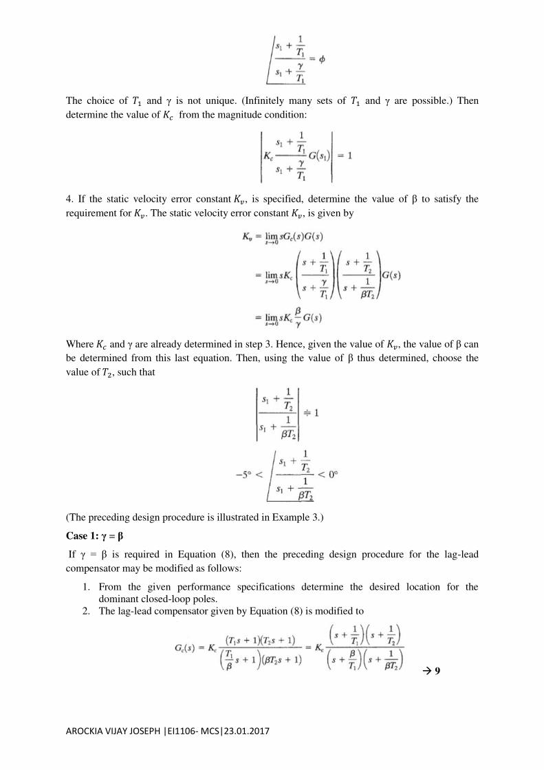
The choice of 𝑇 and is not unique. (Infinitely many sets of 𝑇 and are possible.) Then

determine the value of from the magnitude condition:

4. If the static velocity error constant 𝑣, is specified, determine the value of to satisfy the

requirement for 𝑣. The static velocity error constant 𝑣, is given by

Where and are already determined in step 3. Hence, given the value of 𝑣, the value of can

be determined from this last equation. Then, using the value of thus determined, choose the

value of 𝑇 , such that

(The preceding design procedure is illustrated in Example 3.)

Case 1: =

If = is required in Equation (8), then the preceding design procedure for the lag-lead

compensator may be modified as follows:

1. From the given performance specifications determine the desired location for the

dominant closed-loop poles.

2. The lag-lead compensator given by Equation (8) is modified to

9


where > 1. The open-loop transfer function of the compensated system is s)G(s). If

the static velocity error constant is specified, determine the value of constant from

the following equation:

3. To have the dominant closed-loop poles at the desired location, calculate the angle

contribution φ needed from the phase lead portion of the lag-lead compensator.

4. For the lag-lead compensator, we later choose 𝑇 sufficiently large so that

is approximately unity, where s = is one of the dominant closed-loop poles. Determine

the values of 𝑇 and from the magnitude and angle conditions:

5. Using the value of just determined, choose 𝑇 so that

The value of 𝑇 the largest time constant of the lag-lead compensator, should not be too

large to be physically realized. (An example of the design of the lag-lead compensator

when = is given in Example 4.)


Example 3: Consider the following system with a feed forward transfer function,

The desired locations for the dominant closed-loop poles are at

It is desired to make the damping ratio of the dominant closed-loop poles equal to 0.5 and

to increase the undamped natural frequency to 5 rad/sec and the static velocity error

constant to 80 − . Design an appropriate compensator to meet all the performance

specifications.




Example 4: Consider the following system with a feed forward transfer function,

The desired locations for the dominant closed-loop poles are at

It is desired to make the damping ratio of the dominant closed-loop poles equal to 0.5 and

to increase the undamped natural frequency to 5 rad/sec and the static velocity error

constant to 80 − . Design an appropriate compensator to meet all the performance

specifications.




Control system design via frequency response

The ultimate aim of study into control system analysis is to use the insight gained for controller design.

That is to select an appropriate compensator type and tune the parameters of that compensator so that the

performance of the system closed-loop response is good.

1.5 The relationship between the system closed loop performance and open loop

frequency response function

The closed loop system performance is concerned with stability, transient response, and steady-state error.

These can all be related to the system open loop frequency response function.

The Nyquist criterion tells us how to determine if a system is stable. Typically, an open-loop stable system

is stable in closed loop if the open-loop magnitude frequency response has a gain of less than 0dB at the

frequency where the phase frequency response is 180 degree.

The transient response is normally described by the percent overshoot and settling time or peak time of the

system response to a step input as shown in the figure below.

The percent overshoot can be related to the phase margin (PM) of the system open loop

frequency response. The setting time and peak time describe the speed of the system response

and directly relate to the bandwidth 𝜔 𝑊 of the system closed loop frequency response which

could be determined from the system open loop frequency response function.

We can therefore achieve a desired system transient response via designing an appropriate open

loop frequency response function. The basic principle for this design is to reach a good

phase/gain margins (45°< phase margins <60° or gain margin->6-10dB) and a sufficient big

bandwidth for the open loop FRF. The good phase/gain margins correspond to desired percent

overshoot, and the bigger the bandwidth is, the faster the speed of the system response will be.

Steady-state errors can be improved by increasing the low frequency magnitude of the open loop

frequency response function, even if the high frequency magnitude response is attenuated. See a

simple illustration in the space below for why.

Generally 𝑦 𝑗𝜔 = 𝑗𝜔 𝑗𝜔+ 𝑗𝜔 𝑗𝜔 𝑗𝜔

For a step input and at the steady state,

𝑦 = 𝑦∞ = 𝑌 𝑗𝜔 |𝜔= = 𝜔 𝜔+ 𝜔 𝜔 |𝜔= r


Note: The above are the basic facts underlying our design for stability, transient response, and

steady state error using frequency response methods. The Nyquist criterion and the Nyquist

diagram compose the underlying theory behind the design process.

1.6. Design via gain adjustment

Consider the adjustment of the gain of a position control system the open loop transfer function

of which is H s = + +

The objective is to achieve a desired transient response which corresponds to a 60 degree phase

margin. The bode plots of the system when K=1 is____________________.

To achieve this objective, at the phase margin frequency where | 𝑗𝜔 𝑗𝜔 | = , , the phase

of 𝑗𝜔 𝑗𝜔 should be ∠ 𝑗𝜔 𝑗𝜔 = − ° + ° = − °

and it can be observed from the Bode plots above that for this purpose the gain of the system

should be increased by 54.8dB. That is 20logK=54.8 so = . ⁄ = .

Under this K, the Bode plots of the system are given below indicating that the design

requirement has been achieved.

This is a successful example. But in other cases, although an adjustment of the gain can

achieve a good PM, hence a good transient response, the simple design may impair the

system Steady state behaviour.

Consider another example where = + +

The objective is again to achieve a desired transient response corresponding to a 60 degree

phase margin. The Bode plot of the system when K-1 is as below.

It can be observed from the plot that to reach 60 degree PM the gain of the system have to be

reduced by 11.6dB, that is,

20 log K = -11.6 K = 0.2630

In this case the Bode plot of the system is as follows indicating that the steady state

performance of the original system has been impaired although a desired transient

performance is achieved.

A solution to this problem is to introduce Lag compensation.


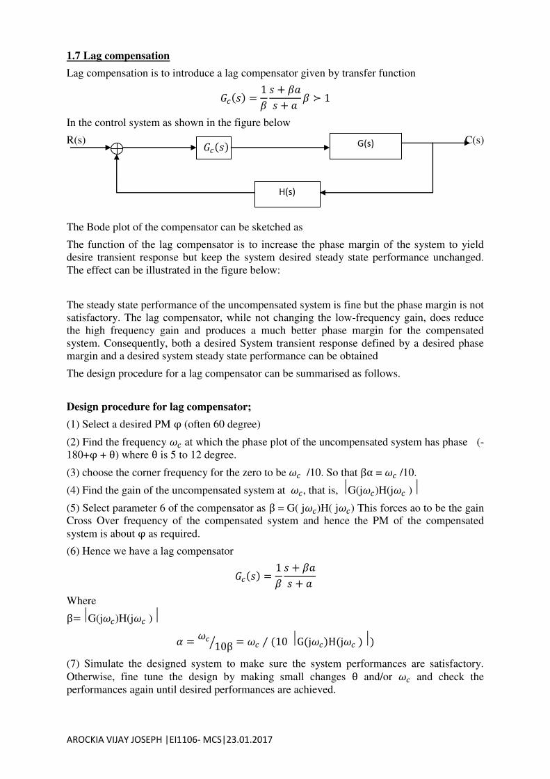
1.7 Lag compensation

Lag compensation is to introduce a lag compensator given by transfer function = ++ ≻

In the control system as shown in the figure below

R(s) C(s)

The Bode plot of the compensator can be sketched as

The function of the lag compensator is to increase the phase margin of the system to yield

desire transient response but keep the system desired steady state performance unchanged.

The effect can be illustrated in the figure below:

The steady state performance of the uncompensated system is fine but the phase margin is not

satisfactory. The lag compensator, while not changing the low-frequency gain, does reduce

the high frequency gain and produces a much better phase margin for the compensated

system. Consequently, both a desired System transient response defined by a desired phase

margin and a desired system steady state performance can be obtained

The design procedure for a lag compensator can be summarised as follows.

Design procedure for lag compensator;

(1) Select a desired PM φ (often 60 degree)

(2) Find the frequency 𝜔 at which the phase plot of the uncompensated system has phase (-

180+φ + θ) where θ is 5 to 12 degree.

(3) choose the corner frequency for the zero to be 𝜔 /10. So that = 𝜔 /10.

(4) Find the gain of the uncompensated system at 𝜔 , that is, G(j𝜔 )H(j𝜔 )

(5) Select parameter 6 of the compensator as = G( j𝜔 )H( j𝜔 ) This forces ao to be the gain

Cross Over frequency of the compensated system and hence the PM of the compensated

system is about φ as required.

(6) Hence we have a lag compensator = ++

Where =G(j𝜔 )H(j𝜔 ) = 𝜔 ⁄ = 𝜔 ⁄ G j𝜔 H j𝜔

(7) Simulate the designed system to make sure the system performances are satisfactory.

Otherwise, fine tune the design by making small changes θ and/or 𝜔 and check the

performances again until desired performances are achieved.

G(s)

H(s)


Note:

1) The 5 to 12 degree phase θ is introduced to compensate for the fact that the phase

of the lag compensator may still contribute anywhere from -5 to -12 degree of phase

at the phase margin (gain cross over) frequency

2) Choosing the corner frequency for the zero to be 𝜔 /10 is to ensure a small effect

of the compensator on the phase of the system at the gain cross over frequency 𝜔 .

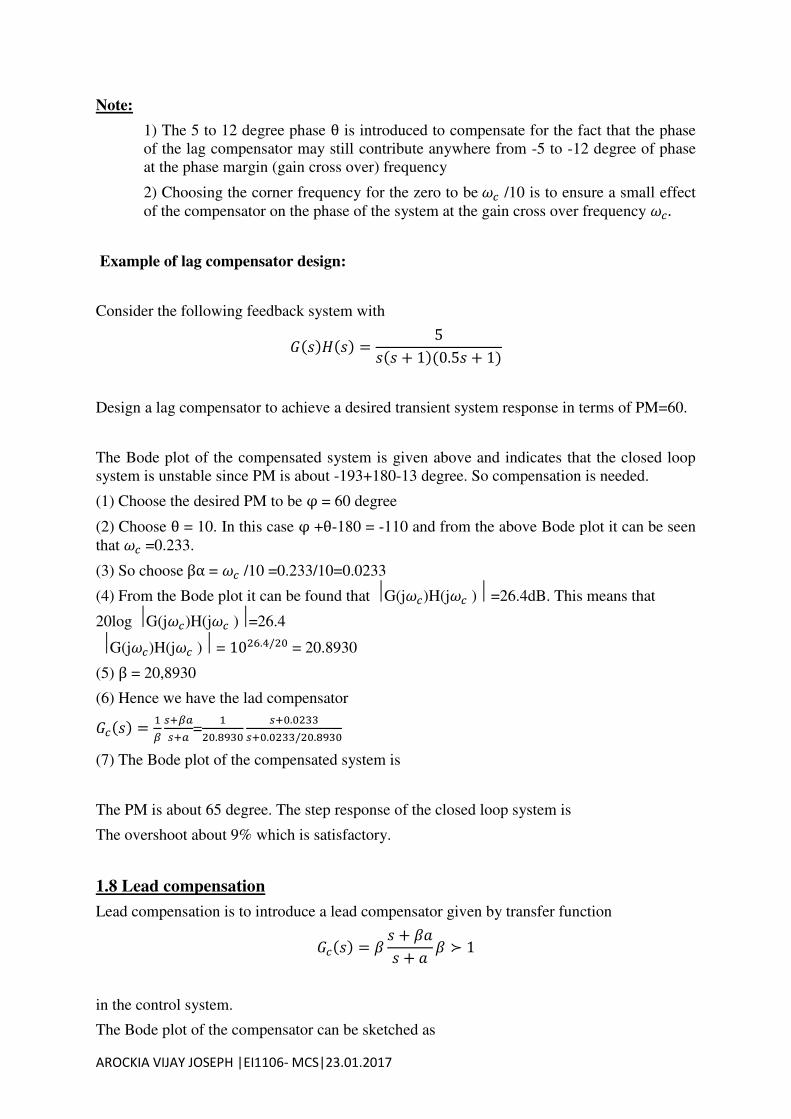
Example of lag compensator design:

Consider the following feedback system with = + . +

Design a lag compensator to achieve a desired transient system response in terms of PM=60.

The Bode plot of the compensated system is given above and indicates that the closed loop

system is unstable since PM is about -193+180-13 degree. So compensation is needed.

(1) Choose the desired PM to be φ = 60 degree

(2) Choose θ = 10. In this case φ +θ-180 = -110 and from the above Bode plot it can be seen

that 𝜔 =0.233.

(3) So choose = 𝜔 /10 =0.233/10=0.0233

(4) From the Bode plot it can be found that G(j𝜔 )H(j𝜔 ) =26.4dB. This means that

20log G(j𝜔 )H(j𝜔 )=26.4

G(j𝜔 )H(j𝜔 ) = . / = 20.8930

(5) = 20,8930

(6) Hence we have the lad compensator = + 𝑎+𝑎 = . + .+ . / .

(7) The Bode plot of the compensated system is

The PM is about 65 degree. The step response of the closed loop system is

The overshoot about 9% which is satisfactory.

1.8 Lead compensation

Lead compensation is to introduce a lead compensator given by transfer function = ++ ≻

in the control system.

The Bode plot of the compensator can be sketched as


When a system has a desired steady state performance and a satisfactory or acceptable phase

margin but a smaller bandwidth hence a slower response speed, a lead compensator may be

introduced to improve the performance. The function of a lead compensator in such case is to

maintain desired steady state performance, keep or even further improve the system phase

margin, and at the same time achieve a faster speed for the system response. The effect is

illustrated in the figure below.

The uncompensated System has a relatively small (may be acceptable may not depending on

design requirements) phase margin and a low phase margin frequency hence a small

bandwidth that implies a slow response speed. Using a lead compensator, the phase angle plot

(compensated system) is raised for high frequencies, At the same time, the gain crossover

frequency in the magnitude plot is increased. These effects yield a similar or larger phase

margin, a higher phase margin frequency, and a larger bandwidth but keep the steady state

gain unchanged. Therefore the compensated system has not only a good steady state

performance but also has a transient response which is "" terms of both percent overshoot and

response speed.

The design of a lead compensator is more complicated than the design for the lag. We need to

first derive the maximum phase of the compensator and the frequency where the maximum

phase is reached.

From ∠ 𝑗𝜔 = − tan− 𝜔 + tan− 𝜔

it is known that the maximum phase is

max {∠ 𝑗𝜔 } = tan− −√

This is reached at 𝜔 = 𝜔𝑚𝑎𝑥 = √

and at frequency 𝑗𝜔 = √ 𝜔2𝑚𝑎𝑥+𝑎2𝜔2𝑚𝑎𝑥+ 2 2 = √ 𝑎2+𝑎2𝑎2+ 2 2 = √

Based on the above basic relationships, we have the following design procedure for the lead

compensator.

Design procedure for lead compensator:

(1) Selecta desired PM φ (often 60 degree) and determine the value of from the equation Φ-𝜑 + 𝜃 = max {∠ 𝑗𝜔 } = tan− −√

where 𝜑 is the phase margin of the uncompensated system and 0 is a correction factor to be

adjusted during the design

(2) Determine the new phase margin frequency , by finding where the uncompensated system’s

magnitude curve is the negative of the lead compensator's magnitude at the peak of the

compensator's phase curve, In other Words, find the frequency where G(j𝜔 )H(j𝜔 )= /√ and select this frequency to be the new phase margin or gain cross over frequency (0.

(3) Determine a from 𝜔 = √

(4) Hence we have a lead compensator = ++


Where tan− −√ = Φ-𝜑 + 𝜃 G(j𝜔 )H(j𝜔 )= /√ , and = 𝜔𝑐√


Otherwise, redesign if necessary to meet requirements,

Note: θ is normally chosen to be 5 to 12 degree because the addition of the lead compensator

shifts the gain crossover frequency to the right and decrease the phase margin.

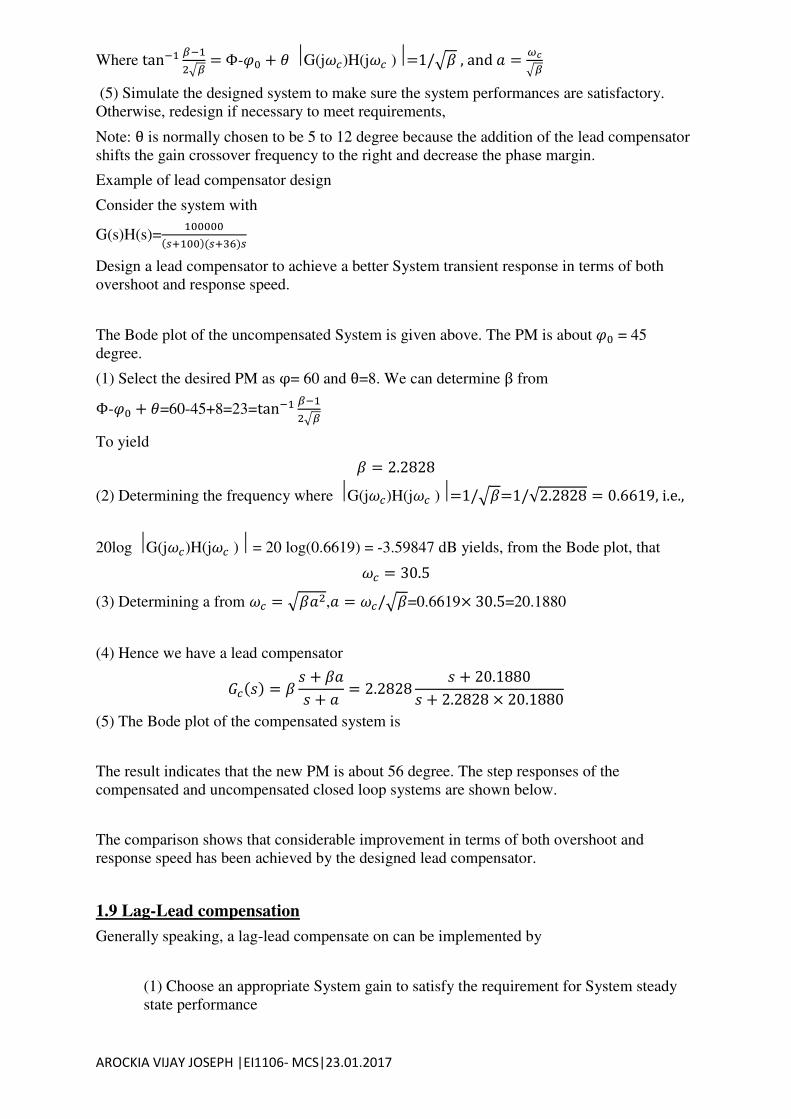
Example of lead compensator design

Consider the system with

G(s)H(s)= + +

Design a lead compensator to achieve a better System transient response in terms of both

overshoot and response speed.

The Bode plot of the uncompensated System is given above. The PM is about 𝜑 = 45

degree.

(1) Select the desired PM as φ= 60 and θ=8. We can determine from Φ-𝜑 + 𝜃=60-45+8=23=tan− −√

To yield = .

(2) Determining the frequency where G(j𝜔 )H(j𝜔 )= /√ =1/√ . = . , i.e.,

20log G(j𝜔 )H(j𝜔 ) = 20 log(0.6619) = -3.59847 dB yields, from the Bode plot, that 𝜔 = .

(3) Determining a from 𝜔 = √ , = 𝜔 /√ =0.6619× . =20.1880

(4) Hence we have a lead compensator = ++ = . + .+ . × .

(5) The Bode plot of the compensated system is

The result indicates that the new PM is about 56 degree. The step responses of the

compensated and uncompensated closed loop systems are shown below.

The comparison shows that considerable improvement in terms of both overshoot and

response speed has been achieved by the designed lead compensator.

1.9 Lag-Lead compensation

Generally speaking, a lag-lead compensate on can be implemented by

(1) Choose an appropriate System gain to satisfy the requirement for System steady

state performance


(2) Design the lag compensation to lower the high frequency gain and stabilize the

System.

(3) Design the lead compensation to meet the phase margin requirement and increase

the system response speed.

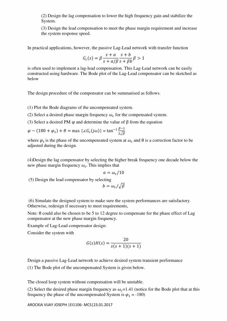
In practical applications, however, the passive Lag-Lead network with transfer function = ++ / ++ >

is often used to implement a lag-lead compensation. This Lag-Lead network can be easily

constructed using hardware. The Bode plot of the Lag-Lead compensator can be sketched as

below

The design procedure of the compensator can be summarised as follows.

(1) Plot the Bode diagrams of the uncompensated system.

(2) Select a desired phase margin frequency 𝜔 for the compensated system.

(3) Select a desired PM φ and determine the value of from the equation 𝜑 − + 𝜑 + 𝜃 = max {∠ 𝑗𝜔 } = tan− −√

where 𝜑 is the phase of the uncompensated system at 𝜔 and θ is a correction factor to be

adjusted during the design.

(4)Design the lag compensator by selecting the higher break frequency one decade below the

new phase margin frequency 𝜔 . This implies that = 𝜔 /

(5) Design the lead compensator by selecting = 𝜔 /√


Otherwise, redesign if necessary to meet requirements,

Note: θ could also be chosen to be 5 to 12 degree to compensate for the phase effect of Lag

compensator at the new phase margin frequency.

Example of Lag-Lead compensator design:

Consider the system with = + +

Design a passive Lag-Lead network to achieve desired system transient performance

(1) The Bode plot of the uncompensated System is given below.

The closed loop system without compensation will be unstable.

(2) Select the desired phase margin frequency as 𝜔 =1.41 (notice for the Bode plot that at this

frequency the phase of the uncompensated System is 𝜑 = -180)


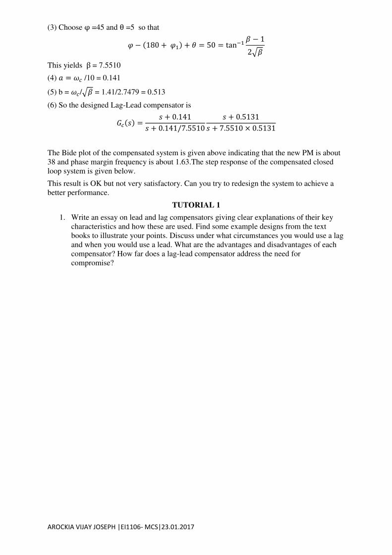
(3) Choose φ =45 and θ =5 so that 𝜑 − + 𝜑 + 𝜃 = = tan− −√

This yields = 7.5510

(4) = 𝜔 /10 = 0.141

(5) b = 𝜔 /√ = 1.41/2.7479 = 0.513

(6) So the designed Lag-Lead compensator is = + .+ . / . + .+ . × .

The Bide plot of the compensated system is given above indicating that the new PM is about

38 and phase margin frequency is about 1.63.The step response of the compensated closed

loop system is given below.

This result is OK but not very satisfactory. Can you try to redesign the system to achieve a

better performance.

TUTORIAL 1

1. Write an essay on lead and lag compensators giving clear explanations of their key

characteristics and how these are used. Find some example designs from the text

books to illustrate your points. Discuss under what circumstances you would use a lag

and when you would use a lead. What are the advantages and disadvantages of each

compensator? How far does a lag-lead compensator address the need for

compromise?


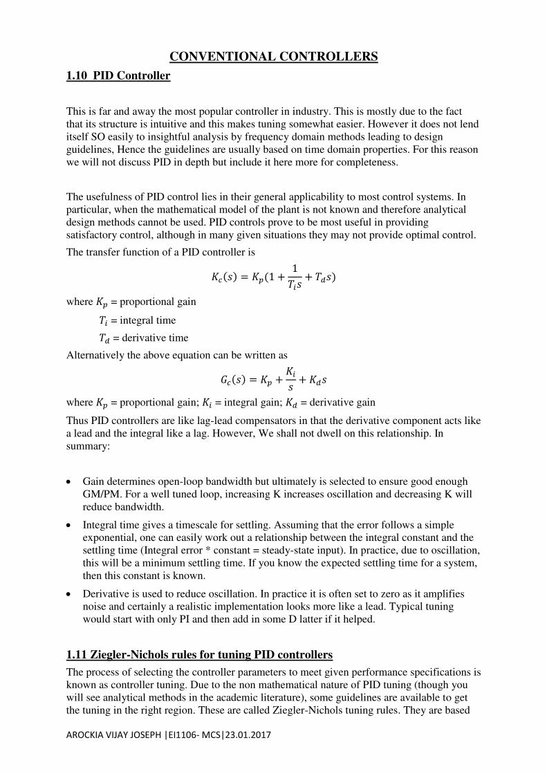
CONVENTIONAL CONTROLLERS

1.10 PID Controller

This is far and away the most popular controller in industry. This is mostly due to the fact

that its structure is intuitive and this makes tuning somewhat easier. However it does not lend

itself SO easily to insightful analysis by frequency domain methods leading to design

guidelines, Hence the guidelines are usually based on time domain properties. For this reason

we will not discuss PID in depth but include it here more for completeness.

The usefulness of PID control lies in their general applicability to most control systems. In

particular, when the mathematical model of the plant is not known and therefore analytical

design methods cannot be used. PID controls prove to be most useful in providing

satisfactory control, although in many given situations they may not provide optimal control.

The transfer function of a PID controller is = 𝑝 + 𝑇 + 𝑇

where 𝑝 = proportional gain 𝑇 = integral time 𝑇 = derivative time

Alternatively the above equation can be written as = 𝑝 + +

where 𝑝 = proportional gain; = integral gain; = derivative gain

Thus PID controllers are like lag-lead compensators in that the derivative component acts like

a lead and the integral like a lag. However, We shall not dwell on this relationship. In

summary:

Gain determines open-loop bandwidth but ultimately is selected to ensure good enough

GM/PM. For a well tuned loop, increasing K increases oscillation and decreasing K will

reduce bandwidth.

Integral time gives a timescale for settling. Assuming that the error follows a simple

exponential, one can easily work out a relationship between the integral constant and the

settling time (Integral error * constant = steady-state input). In practice, due to oscillation,

this will be a minimum settling time. If you know the expected settling time for a system,

then this constant is known.

Derivative is used to reduce oscillation. In practice it is often set to zero as it amplifies

noise and certainly a realistic implementation looks more like a lead. Typical tuning

would start with only PI and then add in some D latter if it helped.

1.11 Ziegler-Nichols rules for tuning PID controllers

The process of selecting the controller parameters to meet given performance specifications is

known as controller tuning. Due to the non mathematical nature of PID tuning (though you

will see analytical methods in the academic literature), some guidelines are available to get

the tuning in the right region. These are called Ziegler-Nichols tuning rules. They are based


on a target of 25% maximum overshoot in Step response for a 2nd

order system. However it is

recognised that many real systems can be approximated quite well by a 2nd order system, and

hence these rules tend to work quite well. Fine tuning is usually required.

Remark: ZN tuning will not work on all processes, for instance they do not apply to unstable

plant. In such cases more insight and trial and error may be required. Typically (for stable

processes) one could start with a low gain PI and gradually up the tuning. Unstable processes

need high gain control and a generic Solution cannot be given.

First Method. (Open-loop method)

In this method, we obtain experimentally the response of the plant to a unit-step input.

If such a response curve looks like a an S-shaped curve (i.e., it involves no integrators or

dominant complex conjugate poles), then the curve may be characterised by a delay time L

(the time before the output changes significantly) and a time constant T (the time it takes

from it starts moving to when it is close to the steady-value). The transfer function 𝑅 may

then be approximated by a first-order system with a transport lag. 𝐶𝑅 = −𝐿𝑇 +

In this case, the Ziegler-Nichols tuning rule is given by the following table.

Type of Controller Kp Ti Td

P 𝑇

∞ 0

PI . 𝑇 .

0

PID . 𝑇

2L 0.5L

Second Method. (Closed-loop method)

First, use the proportional control action only, increase K to a critical value where the output

first exhibits sustained oscillations with a period P. (From root-loci this implies that 2 poles

are crossing from the LHP to the RHP.) In this case, the Ziegler-Nichols tuning rule is given

by the following table.

Type of Controller Kp Ti Td

P 0.5K ∞ 0

PI 0.45K P/1.2 0

PID 0.6K P/2 P/8

Ziegler-Nichols tuning rules (and other tuning rules presented in the literature) have been

Widely used to tune PID controllers in process control systems where the plant dynamics are

not precisely known. Over many years, such tuning rules proved to be very useful. If the

plant dynamics are known, many analytical and graphical approaches to the design of PID

controllers are available in addition to Ziegler-Nichols tuning rules.


1.12 More intuitive approaches

Settling time is dictated by the size of the integral term

1. The steady state input derives solely form the integral component as in steady state the

proportional and derivative terms multiply on Zero (the error being zero in steady state).

2. Assuming an exponential type of response, the integral of the error is given by

approximately

∫−∞ ≈ 𝑇

where r is the setpoint and T the setting time.

3. Hence consistency demands that the following holds for realistic settling times:

𝑇 ≈ (steady state input) =

In conclusion: Given a desired settling time, the required integral constant can be computed.

Rise time is dictated by the proportional gain

4. Given a step change, the error is also, initially a step. For the transient stage the integral

term will be negligible as this depends upon an area which is necessarily small for small

times.

5.Hence the initial input is given by = 𝑝

where r is the set point.

6. Given a view as to how aggressive the controller is allowed to be, that is limits on u(O) for

given r, one can determine arrange of Values for 𝑝.

7. Clearly rise time is dictated largely by how aggressively the input responds in transients

and this depends solely on the proportional term. For a fast rise time, 𝑝 must be large.

Derivative is used cautiously

Derivative helps to reduce overshoot/oscillation in the ideal case. However it amplifies noise.

Hence in many cases it is omitted altogether. Where it must be used the magnitude allowed

will depend on the SNR (signal to noise ratio).

WARNING: When implementing PID on MATLAB, make sure that the set point does not

pass through the derivative or your results will erroneous and misleading. The derivative of a

step is an impulse, which does not exist in real life but MATLAB happily absorbs this in the

algebra without giving any warnings. Some books make this mistake and hence give

erroneous results.

A better PID implementation is as follows: = 𝑝 + − 𝑦

where e is the error and y the output.







EVEN SEM 2017 - SRM Institute of Science and · PDF filearockia vijay joseph |ei1106- mcs|23.01.2017 even sem 2017 arockia vijay joseph department of eie, srm university even sem 2017

Documents