epub.uni-regensburg.de · Contents 1 Alloy Solidiﬁcation 11 1.1 Irreversible thermodynamics . . . . . . . . . . . . . . . . . . . . . . . . . . . . . . . . 11 1.1.1 Thermodynamics

Derivation and Analysis of a

Phase Field Model

for Alloy Solidification

Dissertation zur Erlangung des

Doktorgrades der Naturwissenschaften

(Dr. rer. nat.)

der Naturwissenschaftlichen Fakultat I - Mathematik

der Universitat Regensburg

vorgelegt von

Bjorn Stinner

Regensburg, Oktober 2005

Promotionsgesuch eingereicht am 10. Oktober 2005

Die Arbeit wurde angeleitet von Prof. Dr. H. Garcke

Prufungsausschuss: Vorsitzender: Prof. Dr. Jannsen1. Gutachter: Prof. Dr. Garcke2. Gutachter: Priv.-Doz. Dr. Eckweiterer Prufer: Prof. Dr. Finster Zirker

Contents

1 Alloy Solidification 111.1 Irreversible thermodynamics . . . . . . . . . . . . . . . . . . . . . . . . . . . . . . . . 11

1.1.1 Thermodynamics for a single phase . . . . . . . . . . . . . . . . . . . . . . . . 111.1.2 Multi-phase systems . . . . . . . . . . . . . . . . . . . . . . . . . . . . . . . . 151.1.3 Derivation of the Gibbs-Thomson condition . . . . . . . . . . . . . . . . . . . 18

1.2 The general sharp interface model . . . . . . . . . . . . . . . . . . . . . . . . . . . . 241.3 Non-negativity of entropy production . . . . . . . . . . . . . . . . . . . . . . . . . . . 251.4 Calibration . . . . . . . . . . . . . . . . . . . . . . . . . . . . . . . . . . . . . . . . . 28

1.4.1 Phase diagrams . . . . . . . . . . . . . . . . . . . . . . . . . . . . . . . . . . . 281.4.2 Mass diffusion . . . . . . . . . . . . . . . . . . . . . . . . . . . . . . . . . . . 30

2 Phase Field Modelling 332.1 The general phase field model . . . . . . . . . . . . . . . . . . . . . . . . . . . . . . . 342.2 Non-negativity of entropy production . . . . . . . . . . . . . . . . . . . . . . . . . . . 382.3 Examples . . . . . . . . . . . . . . . . . . . . . . . . . . . . . . . . . . . . . . . . . . 39

2.3.1 Possible choices of the surface terms . . . . . . . . . . . . . . . . . . . . . . . 392.3.2 Relation to the Penrose-Fife model . . . . . . . . . . . . . . . . . . . . . . . . 402.3.3 A linearised model . . . . . . . . . . . . . . . . . . . . . . . . . . . . . . . . . 412.3.4 Relation to the Caginalp model . . . . . . . . . . . . . . . . . . . . . . . . . . 422.3.5 Relation to the Warren-McFadden-Boettinger model . . . . . . . . . . . . . . 43

2.4 The reduced grand canonical potential . . . . . . . . . . . . . . . . . . . . . . . . . . 442.4.1 Motivation and introduction . . . . . . . . . . . . . . . . . . . . . . . . . . . 442.4.2 Example . . . . . . . . . . . . . . . . . . . . . . . . . . . . . . . . . . . . . . . 462.4.3 Reformulation of the model . . . . . . . . . . . . . . . . . . . . . . . . . . . . 47

3 Asymptotic Analysis 493.1 Expansions and matching conditions . . . . . . . . . . . . . . . . . . . . . . . . . . . 513.2 First order asymptotics of the general model . . . . . . . . . . . . . . . . . . . . . . 55

3.2.1 Outer solution . . . . . . . . . . . . . . . . . . . . . . . . . . . . . . . . . . . 563.2.2 Inner expansion . . . . . . . . . . . . . . . . . . . . . . . . . . . . . . . . . . . 573.2.3 Jump and continuity conditions . . . . . . . . . . . . . . . . . . . . . . . . . . 593.2.4 Gibbs-Thomson relation and force balance . . . . . . . . . . . . . . . . . . . . 60

3.3 Second order asymptotics in the two-phase case . . . . . . . . . . . . . . . . . . . . . 643.3.1 The modified two-phase model . . . . . . . . . . . . . . . . . . . . . . . . . . 643.3.2 Outer solutions . . . . . . . . . . . . . . . . . . . . . . . . . . . . . . . . . . . 653.3.3 Inner solutions . . . . . . . . . . . . . . . . . . . . . . . . . . . . . . . . . . . 663.3.4 Summary of the leading order problem and the correction problem . . . . . . 69

3.4 Numerical simulations of test problems . . . . . . . . . . . . . . . . . . . . . . . . . . 713.4.1 Scalar case in 1D . . . . . . . . . . . . . . . . . . . . . . . . . . . . . . . . . . 713.4.2 Scalar case in 2D . . . . . . . . . . . . . . . . . . . . . . . . . . . . . . . . . . 743.4.3 Binary isothermal systems . . . . . . . . . . . . . . . . . . . . . . . . . . . . . 75

3

3.4.4 Binary non-isothermal case . . . . . . . . . . . . . . . . . . . . . . . . . . . . 76

4 Existence of Weak Solutions 794.1 Quadratic reduced grand canonical potentials . . . . . . . . . . . . . . . . . . . . . . 81

4.1.1 Assumptions and existence result . . . . . . . . . . . . . . . . . . . . . . . . . 814.1.2 Galerkin approximation . . . . . . . . . . . . . . . . . . . . . . . . . . . . . . 844.1.3 Uniform estimates . . . . . . . . . . . . . . . . . . . . . . . . . . . . . . . . . 864.1.4 First convergence results . . . . . . . . . . . . . . . . . . . . . . . . . . . . . . 894.1.5 Strong convergence of the gradients of the phase fields . . . . . . . . . . . . . 904.1.6 Initial values for the phase fields . . . . . . . . . . . . . . . . . . . . . . . . . 924.1.7 Additional a priori estimates . . . . . . . . . . . . . . . . . . . . . . . . . . . 94

4.2 Linear growth in the chemical potentials . . . . . . . . . . . . . . . . . . . . . . . . . 974.2.1 Assumptions and existence result . . . . . . . . . . . . . . . . . . . . . . . . . 984.2.2 Solution to the perturbed problem . . . . . . . . . . . . . . . . . . . . . . . . 994.2.3 Properties of the Legendre transform . . . . . . . . . . . . . . . . . . . . . . . 1014.2.4 Compactness of the conserved quantities . . . . . . . . . . . . . . . . . . . . . 1044.2.5 Convergence statements . . . . . . . . . . . . . . . . . . . . . . . . . . . . . . 107

4.3 Logarithmic temperature term . . . . . . . . . . . . . . . . . . . . . . . . . . . . . . 1094.3.1 Assumptions and existence result . . . . . . . . . . . . . . . . . . . . . . . . . 1104.3.2 Solution to the perturbed problem . . . . . . . . . . . . . . . . . . . . . . . . 1124.3.3 Estimate of the conserved quantities . . . . . . . . . . . . . . . . . . . . . . . 1144.3.4 Strong convergence of temperature and chemical potentials . . . . . . . . . . 1184.3.5 Convergence statements . . . . . . . . . . . . . . . . . . . . . . . . . . . . . . 122

A Notation 123

B Equilibrium thermodynamics 125

C Facts on evolving surfaces and transport identities 129

D Several functional analytical results 131

4

Introduction

The subject of the present work is the derivation and the analysis of a phase field model to de-scribe solidification phenomena on a microscopic length scale occurring in alloys of iron, aluminium,copper, zinc, nickel, and other materials which are of importance in industrial applications. Me-chanical properties of castings and the quality of workpieces can be traced back to the structure onan intermediate length scale of some µm between the atomic scale of the crystal lattice (typicallyof some nm) and the typical size of the workpiece. This so-called microstructure consists of grainswhich may only differ in the orientation of the crystal lattice, but it is also possible that there aredifferences in the crystalline structure or the composition of the alloy components. In the first casethe system is named homogeneous, in the latter case heterogeneous. The homogeneous parts inheterogeneous systems are named phases. These phases itself are in thermodynamic equilibriumbut the boundaries separating the grains of the present phases are not in equilibrium and compriseexcess free energy. Following [Haa94], Chapter 3, the microstructure is defined to be the totality ofall crystal defects which are not in thermodynamic equilibrium.

The fact that the thermodynamic equilibrium is not attained results from the process of solid-ification. When a melt is cooled down solid germs appear and grow into the liquid phase. Thetype of the solid phase and the evolution of the solid-liquid phase boundaries depends on the localconcentrations of the components and on the local temperature. But also the surface energy ofthe solid-liquid interface plays an important role. Not only the typical size of the microstructure isdetermined by the surface energy. Its anisotropy, together with certain (possibly also anisotropic)mobility coefficients, and the fact that the solid-liquid interface is unstable leads to the formation ofdendrites as in Fig. 1. The properties as the number of tips, the tip velocity, and the tip curvatureare of special interest in materials science.

During the growth, the primary solid phases can meet forming grain boundaries which involvesurface energies of their own. In eutectic alloys, lamellar eutectic growth as in Fig. 2 on the leftcan be observed, i.e., layers of solid phases enriched with two different components grow into amelt of an intermediate composition. The strength and robustness of workpieces thanks to thatfine microstructure make such alloys of particular interest in industry. The typical width of thegrains and its dependence on composition and cooling rate is of interest as well as the appearanceof patterns like, for example, eutectic colonies (cf. Fig. 2 on the right). At an even later stageof solidification, when essentially the whole melt is solidified, coarsening and ripening processesinvolving a motion of the grain boundaries on a larger timescale are observed.

In the following, the distinction between phase and grain will be dropped, and the notation”phase” will be used for an atomic arrangement in thermodynamic equilibrium as well as a domainoccupied by a certain phase, i.e., a grain of the phase. As a consequence, the notation ”phaseboundary” will be used for interfaces separating grains of the same phase, too.

When modelling solidification processes, classically, the occurring phase boundaries are movinghypersurfaces meeting in triple lines or moving curves meeting in triple points if the problem isessentially two dimensional as in thin films. The Gibbs-Thomson condition couples the form andthe motion of the interface to its surface energy and to the local thermodynamic potentials. Inthe Stefan problem (cf. [Dav01], Section 2.2) for a pure material, for example, the Gibbs-Thomsoncondition states that the deviation of the temperature from its equilibrium value u = c(T − Tm)

5

Figure 1: On the left: growth of a primary dendrite with intermediate eutectic microstruc-ture into some hypo-eutectic C2Cl6-CBr4-alloy (Akamatsu and Faivre, picture from http://www.gps.jussieu.fr/ gps/ surfaces/ lamel.htm); on the right: ice crystal (Libbrecht, picture fromhttp:// www.its.caltech.edu/ atomic/ snowcrystals/ photos/ photos.htm)

on the solid-liquid interface (T being the interfacial temperature, Tm the melting temperature, andc some material dependent constant) is proportional to the surface tension σ multiplied with thecurvature κ of the interface,

u = σκ.

In addition, balance equations for the energy and the components must be considered. In thecontext of irreversible thermodynamics (cf. [Mul01], see also Section 1.1.1 for a brief introduction)this leads to diffusion equations for the heat and the components in the pure phases, coupled tojump conditions on the phase boundaries taking, for example, the release of latent heat duringsolidification and the segregation of components into account (cf. [Dav01], Section 3.1). In thealready mentioned Stefan problem the diffusion equation for the heat reads

∂tu = D∆u

with some diffusion coefficient D, and the jump condition on the solid-liquid interface

lvν = [−D∇u] · νwhere the constant l is proportional to the latent heat, ν is a unit normal on the interface, vν isthe velocity of the interface in direction ν, and [·] denotes the jump of the quantity in the bracketswhen crossing the interface in direction ν.

The idea of introducing order parameters enables to state a weak formulation of the free bound-ary problem and, possibly, to solve it (for example, [Luc91] for the Stefan problem). To eachpossible phase an order parameter φ, in the following also called phase field variable, is introducedto describe the presence of the corresponding phase, i.e., in a pure phase the phase field variableof the corresponding phase is one while the other phase field variables vanish, and on the phaseboundaries they are not defined but jump across the interface. As long as the phase field variablesare of bounded variation, the surface energy is given as an integral of terms of their spatial gradientsover the considered domain. In the case of a system with two phases occupying a domain Ω a scalarphase field variable φ ∈ BV (Ω) is sufficient, and the surface energy is then

Esharp =

∫

Ω

σ|∇φ| dx

where |∇φ| dx has to be understood in the sense of a measure with support on the phase bound-ary. Adding further thermodynamic potentials to the energy (depending on the temperature, for

6

Figure 2: On the left: eutectic structures of some Ru-Al-Mo-alloy (Rosset, Cefalu, Varner,Johnson, picture from https:// engineering.purdue.edu/ MSE/ FACULTY/ RESEARCH FOCUS/Def Fract Ruth.whtml); on the right: eutectic grains, so-called colonies (Akamatsu and Faivre,picture from http:// www.gps.jussieu.fr/ gps/ surfaces/ lamel.htm)

example), the evolution of the phase boundaries can be defined as an appropriate gradient flow ofthe free energy in the isothermal case or, with the opposite sign, of the entropy in the general case.

In the phase field approach, a length scale ε smaller than the typical size of the microstructureto be described is introduced. Instead of jumping across the phase boundaries, the phase fieldvariables change smoothly in a transition layer whose thickness is determined by the new smalllength scale ε. This leads to the notion of a diffuse interface. The smooth profiles of the phasefields in the interfacial layer are obtained by replacing the sharp interface energy/entropy by aGinzburg-Landau type energy/entropy involving a gradient term and a multi-well potential w. Inthe case of two phases it may be of the form

Ediffuse =

∫

Ω

(

εσ|∇φ|2 +σ

εw(φ)

)

dx.

In the corresponding gradient flow, leading to systems of Allen-Cahn equations (cf., for example,[TC94]), the gradient term models diffusion trying to smooth out the phase field variables whilethe multi-well potential term is a counter-player and tries to separate the values. Of particularinterest is the limit when the small length scale ε related to the thickness of the interfacial layertends to zero. In quite general settings, the Γ-limit of the Ginzburg-Landau energy is known (cf.[Mod87, BBR05]), and for the time dependent case there are results establishing a relation betweenthe Allen-Cahn equations and motion by curvature. Much less is known in the case that additionalevolution equations are coupled to the Allen-Cahn equations as, for example, balance equations inmodels for solidification. Nevertheless, using the method of matched asymptotic expansions, oftena sharp interface model related to the phase field model can be found.

The use of such smoothly varying phase field variables dates back to ideas of van der Waals[vdW83] and Landau and Ginzburg [LG50]. Langer [Lan86] and Caginalp [Cag89] introduced theidea in the context of solidification on which [OKS01] gives a summary. An overview on otherapplications of the phase field approach can be found in [Che02]. The phase field is not always con-sidered as a mathematical device allowing for a reformulation of a free boundary problem. In othermodels, the phase field variables stand for physical quantities as, for example, the concentrationsin the model of Cahn and Hilliard [CH58] or the mass density. There, the phase transitions areregarded as being diffuse from the beginning, i.e., they have a thickness of some atomic layers, andthe sharp interface model is considered as an approximation on a larger length scale.

Independent of the interpretation of the phase field variables and the question whether the diffuseinterface model is the natural one or an approximation of a free boundary problem, one advantage

7

of the phase field approach is that the numerical implementation of phase field models is muchsimpler than of sharp interface models. The fact that phases can disappear and phase boundariescan coalesce must be taken into account. The numerical handling of such singularities is difficultfor the sharp interface model but not impossible (cf. [Sch98]). This problem is overcome in thephase field approach since there are only parabolic differential equations to solve. Furthermore, theextension of the interface by one dimension does not really cause high additional effort as long asadaptive methods are applied since the transition layers where the phase field variables stronglyvary are very thin.

In the following, a short overview on the content of the present work is given. Intentionally, it iskept brief since each chapter starts with a careful and detailed introduction on its goals, difficulties,and results.

In Chapter 1, the sharp interface modelling of solidification in alloy systems is revised. Based onirreversible thermodynamics, the governing set of equations is derived providing a general framework(cf. Section 1.2). The main task is the derivation of the Gibbs-Thomson condition from a localisedgradient flow of the entropy. To obtain a model for a specific material, the framework has to becalibrated by postulating suitable free energy densities for the possible phases and inserting materialproperties and parameters such as the surface energies and diffusivities.

In Chapter 2, a general framework for phase field modelling of solidification is presented. Anentropy functional of Ginzburg-Landau type in the phase field variables plays the central role.Balance equations for the conserved quantities are coupled to a gradient flow like evolution equationfor the phase fields in such a way that an entropy inequality can be derived. The general characterbecomes clear by demonstrating that the governing equations of earlier models are obtained byappropriate calibration. For the following analysis it turns out that the so-called reduced grandcanonical potential density is a good thermodynamic quantity to formulate the general model. Itis defined to be the Legendre transform of the negative entropy density.

The relation between the phase field model of the second chapter and the sharp interface modelof the first chapter in the sense of a sharp interface limit is shown in Chapter 3. First, the procedureof matching asymptotic expansions is outlined. Afterwards, the main result on the relation is statedand proven. The quality of the approximation is of interest, too, and it is demonstrated that incertain cases a higher order approximation is possible taking additional correction terms in thephase field model into account. Numerical simulations support the theoretical results.

Chapter 4 is dedicated to the rigorous analysis of the partial differential equations of the phasefield model. The parabolic system has the structure

∂tb(u, φ) = ∇ · L∇u,

∂tφ = ∇ · a′(∇φ) − w′(φ) + g(u, φ)

for a function u related to thermodynamic quantities and a set of phase field variables φ. Thefirst equation describes conservation of conserved quantities while the second one is the gradientflow of the entropy. The function b is the derivative of the reduced grand canonical potential ψwhich is a convex function with respect to u, i.e., b is monotone in u, and also the coupling termg is related to ψ. Existence of weak solutions to the parabolic system of equations is shown. Thefocus lies on tackling difficulties caused by the growth properties of the reduced grand canonicalpotential ψ in u, namely, potentials ψ involving terms like − ln(−u) or of at most linear growth inu are of interest. The idea is to use a perturbation technique. The perturbed problem is solvedmaking a Galerkin ansatz. The main task is then to derive suitable estimates and, based on theestimates, to develop and apply appropriate compactness arguments in order to go to the limit asthe perturbation vanishes.

8

Acknowledgement

I want to thank everyone who contributed to this work and supported me to finish it. My deepestthanks go to my supervisor Harald Garcke for his ideas and help to tackle all the challenges.Furthermore, I thank Britta Nestler and Christof Eck for the fruitful discussions on solidificationphenomena and applications and, respectively, on the existence theory of weak solutions to partialdifferential equations.

I gratefully acknowledge the German Research Foundation (DFG) for the financial supportwithin the priority program ”Analysis, Modeling and Simulation of Multiscale Problems”.

9

10

Chapter 1

Alloy Solidification

In applications, the production of certain microstructural morphologies in alloys is often achievedby imposing appropriate conditions just before and during the solidification process. In order toget a deeper understanding of the process, the scientific challenge is to describe the microstructureformation with a mathematical model, where the imposed conditions enter as initial and boundaryvalues or as additional forces and parameters in the equations governing the evolution. Startingfrom thermodynamic principles for irreversible processes, a framework for continuum modelling ofalloy solidification is derived in Section 1.1.

Balancing the conserved quantities energy and mass respectively concentrations of the compo-nents yields diffusion equations in the bulk phases as well as continuity and jump conditions on themoving phase boundaries. A coupling of the phase boundary motion to the thermodynamic quan-tities of the adjacent phases, the Gibbs-Thomson condition, is derived by localising an appropriategradient flow of the entropy. For this purpose, variations of the entropy by deforming the interfacein a small ball around a point on the phase boundary are considered. Since only variations areadmissible such that the energy and mass remain conserved, the motion law is obtained by lettingthe radius of the small ball converge to zero after suitable rescaling.

It turns out that the balance equations and the Gibbs-Thomson condition, together with certainangle conditions in junctions where several phases meet and which are due to local force balance,enable to show that local entropy production is non-negative and to derive an entropy inequality.This is presented in Section 1.3 after stating the total set of governing equations in Section 1.2.

Finally, in Section 1.4, it is discussed how material parameters can enter the framework such thata certain alloy is described. This step is called calibration. Bulk material properties and physicalparameters as latent heats and melting temperatures of the components can be taken into accountby postulating appropriate free energies of the possible phases. Their relation to the phase diagramdescribing the solidification behaviour of the considered alloy is briefly clarified. Experimentallymeasurable diffusion coefficients can enter the equations via suitable definition of the fluxes for theconserved quantities.

In this chapter, partial derivatives sometimes are denoted by subscripts after a comma. Forexample, s,e is the partial derivative of the function s = s(e, c) with respect to the variable e.

1.1 Irreversible thermodynamics

1.1.1 Thermodynamics for a single phase

An alloy of N ∈ N components occupying an open domain Ω ∈ Rd during some time interval

I = (0, T ) is considered. In applications d = 3, but in the following chapters sometimes problemsare examined which effectively are one or two dimensional, hence d ∈ 1, 2, 3. There are nophase boundaries present, only the distributions of temperature and composition of the alloy are

11

CHAPTER 1. ALLOY SOLIDIFICATION

of interest. The following assumptions are made:

S1 The system is closed, there is no mass flux across the external boundary ∂Ω.

S2 The pressure is constant.

S3 The only transport mechanism is diffusion. There are no forces present leading to flows ordeformations.

S4 The mass density is constant.

The domain Ω remains undeformed during evolution. In applications, the changes in pressureor volume are often small and can be neglected (cf. [Haa94], Section 5.1) which motivates thesecond assumption. Models with constant mass density like the Stefan problem of the Introductionhave been very successfully applied to describe microstructural evolution. But other effects as, forexample, convection in liquid phases, can strongly influence the growing structures (cf. [Dav01]).The applicability of the model presented in the following is therefore restricted to cases where sucheffects can be neglected. Before deriving the governing set of equations some objects are definedfor later use.

1.1 Definition For K ∈ N define the sets

HΣK :=

v ∈ RK :

K∑

i=1

vi = 1

, (1.1a)

ΣK :=

v ∈ HΣK : vi ≥ 0 ∀i

. (1.1b)

The tangent space on HΣK can be naturally identified in every point v ∈ HΣK with the subspace

TvHΣK ∼= TΣK :=

w ∈ RK :

K∑

i=1

wi = 0

. (1.1c)

The map PK : RK → TΣK is the orthogonal projection given by

PKw =(

wk − 1

K

K∑

l=1

wl

)K

k=1=

(

IdK − 1

K1K ⊗ 1K

)

w

where 1K = (1, . . . , 1) ∈ RK and IdK is the identity on R

K .

Observe that IdK − 1K 1K ⊗ 1K is symmetric and PKw = w for all w ∈ TΣK .

By the first law of thermodynamics, energy and mass are conserved quantities. By e or c0 theinternal energy density (with respect to volume) is denoted. Let N be the number of components.Then ci is the concentration of component i ∈ 1, . . . , N. Writing c = (c1, . . . cN ), the (mass)concentrations are demanded to fulfil the constraint

c ∈ ΣN . (1.2)

Following [Mul01], Section 11.2, the evolution is governed by balance equations for the conservedquantities. By the above Assumptions S2–S4 they simplify to

∂te = −∇ · J0, ∂tci = −∇ · Ji, 1 ≤ i ≤ N, (1.3)

with fluxes J0 for the energy and Ji for concentration ci. For (1.2) being fulfilled the constraint

N∑

i=1

Ji = 0 (1.4)

12

1.1. IRREVERSIBLE THERMODYNAMICS

is imposed. In thermodynamics of irreversible processes the relations between the fields are basedon the principle of local thermodynamic equilibrium. In the present situation the entropy densitys is a function of the conserved quantities. Its derivatives are the inverse temperature and thechemical potential difference reduced by the temperature (see Appendix B), i.e.,

s = s(e, c) and ds =1

Tde +

−µ

T· dc.

By µi the chemical potential divided by the (by Assumption S4 constant) mass density correspond-ing to component i is denoted. In the above equation the identity µ = PNµ was used whereµ = (µ1, . . . , µN ). The scalar field T is the temperature. The fluxes are postulated to be linear

combinations of the thermodynamic forces ∇ 1T and ∇−µj

T , 1 ≤ j ≤ N , i.e.,

Ji = Li0 ∇1

T+

N∑

j=1

Lij ∇−µj

T, 0 ≤ i ≤ N (1.5)

with coefficients Lij which may depend on the thermodynamic potentials 1T and −µ

T or on theconserved quantities e and c. This phenomenological theory was already introduced in [Ons31]. Itis assumed that

L = (Lij)Ni,j=0 is positive semi-definite. (1.6a)

In Section 1.3 it is shown in a more general context that then local entropy production indeed isnon-negative. To fulfil (1.4) it is required that

N∑

i=1

Lij = 0, ∀j ∈ 1, . . . , N. (1.6b)

Onsager’s law of reciprocity states the symmetry of L and can be proven and experimentallyobserved if the fluxes and forces are independent (cf. [KY87], Section 3.8). The above fluxes arenot independent by the constraint (1.4). But even in the present case Onsager’s law can be shownto hold by a certain choice of the coefficients (see [KY87], Section 4.2, and the reference therein;there the calculation is performed for the isothermal case, but another additional independent forcecan be taken into account without any problem). A simple calculation shows that then due to thesymmetry of the matrix (Lij)i,j

N∑

j=1

Lij ∇−µj

T=

N∑

j=1

Lij ∇−µj

T.

Another short calculation, more precisely considering Ji−JN , shows that the definition of the fluxesas above is equivalent to the definition in [Mul01], Section 11.2.

The equations (1.3) are coupled to initial conditions at t = 0 and boundary conditions on theexternal boundary ∂Ω. As the system is closed it holds that Ji · νext = 0 for all i ∈ 1, . . . , N, νext

is the external unit normal. If not otherwise stated the same is assumed for the energy flux, i.e.,the system is adiabatic.

The equations (1.3) can also be interpreted as gradient flow of the entropy with respect to aweighted H−1-product. Let

M : L1(Ω, R × TΣN ) → R × TΣN , M(f) =(

0, —

∫

Ω

f1(x) dx, . . . , —

∫

Ω

fN (x) dx)

and consider the following problem: Given some function f ∈ L2(Ω, R×TΣN) find h ∈ H1,2(Ω, R×TΣN ) with M(h) = 0 such that

∫

Ω

∇v : L∇h :=

∫

Ω

N∑

i,j=0

∇vi · Lij∇hj =

∫

Ω

v · f (1.7)

13


for all test functions v ∈ H1,2(Ω, R × TΣN ) with M(v) = 0. Using the Lax-Milgram theorem(cf. [Alt99], Theorem 4.2) it can be shown that this problem has a unique solution provided thefollowing conditions are satisfied:

L1 The functions Lij are essentially bounded, i.e., Lij ∈ L∞(Ω), 0 ≤ i, j ≤ N ,

L2 the core of the matrix L = (Lij)Ni,j=0 is the space (R × TΣN )⊥, i.e., the space spanned by

(0, 1, . . . , 1) ∈ RN+1.

If L depends on e, c, T , or µ then, given a situation in form of measurable fields (e, c, T, µ), itis assumed that the Lij(e, c, T, µ) fulfils these properties. Observe that by the second assumptionthe matrix L is positive definite when restricted on R × TΣN so that the left hand side of (1.7) iscoercive. Let G be the operator that assigns to each f ∈ L2(Ω, R × TΣN ) the solution h of (1.7).By

(f1, f2)L := (G(f1), f2)L2 (1.8)

a scalar product on L2(Ω, R × TΣN ) is well-defined. Indeed, the symmetry follows from the sym-metry of L and

(f1, f2)L =

∫

Ω

G(f1) · f2 =

∫

Ω

∇G(f1) : L∇G(f2)

=

∫

Ω

∇G(f2) : L∇G(f1) =

∫

Ω

G(f2) · f1 = (f2, f1)L,

and the positivity from assumption L2.

If the system is isolated mass and energy in the whole system are constant, i.e., M((e, c)T (t)) =M((e, c)T (t = 0)) and M(∂t(e, c)T (t)) = 0 for all t ∈ I. Therefore, when computing the variationof the entropy, only directions v ∈ L2(Ω, R × TΣN ) with M(v) = 0 are allowed. The gradient flowreads

(∂t(e, c)T , v)L =⟨ δS

δ(e, c)(e, c), v

⟩

=

∫

Ω

( 1

T,−µ

T

)T

· v =: −∫

Ω

u · v.

For the second identity the relations s,e = 1T and s,c = −µ

T were used. For some w ∈ L2(Ω, R×TΣN)the function w − M(w) is an allowed test function. By (1.8)

∫

Ω

(

G(∂t(e, c)T ) − M(G(∂t(e, c)T )))

· w =

∫

Ω

G(∂t(e, c)T ) · (w − M(w))

= (∂t(e, c)T , w − M(w))L = −∫

Ω

u · (w − M(w)) = −∫

Ω

(u − M(u)) · w

so that G(∂t(e, c)T ) = −u+M(u−G(∂t(e, c)T )). Since ∇M(G(∂t(e, c)T )) = 0 equation (1.7) yieldsfor v ∈ L2(Ω, R × TΣN ) with M(v) = 0 the identity

∫

Ω

v · ∂t(e, c)T =

∫

Ω

∇v : L∇G(∂t(e, c)T ) =

∫

Ω

∇v : L∇(−u).

The corresponding strong formulation is (1.3) with the fluxes defined in (1.5).

If the system not isolated but closed and, for example, Dirichlet boundary conditions are imposedfor the temperature then of course a different solution space must be considered for problem (1.7),whence the above facts and conclusions read different.

14


1.1.2 Multi-phase systems

Let M ∈ N be the number of possible phases. The domain Ω is now decomposed into subdomainsΩ1(t), . . . , ΩM (t), t ∈ I, which are called phases (and, more precisely, correspond to grains inapplications; see the discussion in the Introduction). The phases are not necessarily connectedbut it is assumed that each one consists of an finite number of connected subdomains. The phaseboundaries

Γαβ(t) := Ωα(t) ∩ Ωβ(t), 1 ≤ α, β ≤ M, α 6= β,

are supposed to be piecewise smoothly evolving points, curves or hypersurfaces, depending on thedimension (cf. Definition C.1 in Appendix C). The unit normal on Γαβ pointing into phase β isdenoted by ναβ . The external boundary of phase Ωα is denoted by

Γα,ext := Ωα(t) ∩ ∂Ω.

If d ≥ 2 the intersections of the curves or hypersurfaces are defined by (for pairwise differentα, β, δ ∈ 1, . . . , M)

Tαβδ(t) := Ωα(t) ∩ Ωβ(t) ∩ Ωδ(t).

Besides the phase boundaries can hit the external boundary. The sets of these points are denotedby

Tαβ,ext(t) := Ωα(t) ∩ Ωβ(t) ∩ ∂Ω.

If d = 2 then Tαβδ is a set of triple junctions, i.e., piecewise smoothly evolving points. If d = 3 triplelines can appear which are piecewise smoothly evolving curves. The triple lines can intersect andform quadruple junctions. Then the following sets are well-defined for pairwise different α, β, δ, ζ ∈1, . . . , M:

Qαβδζ(t) := Ωα(t) ∩ Ωβ(t) ∩ Ωδ(t) ∩ Ωζ(t).

Besides the triple lines can hit the external boundary. The sets of these points are denoted by

Qαβδ,ext(t) := Ωα(t) ∩ Ωβ(t) ∩ Ωδ(t) ∩ ∂Ω.

1.2 Remark During evolution, it may happen that one of the connected subdomains of a phase oreven a whole phase vanishes, namely if the adjoining phase boundaries coalesce. It is also possiblethat a piece of a phase boundary vanishes so that one of the sets Tαβδ includes a quadruple pointor line. The latter configuration is not in mechanical equilibrium and will instantaneously split upforming new phase boundaries.

It is supposed that such singularities only occur at finitely many times t ∈ I during the evolution.This is why only piecewise smooth evolution is assumed. The following evolution equations arestated for times at which no singularity occurs.

In each phase Ωα, α ∈ 1, . . . , M, the smooth fields as in the previous Subsection 1.1.1 arepresent. They are denoted by cα

i , eα, µαi , T α and sα (here, α is always an index, no exponent).

Additionally, surface fields on the phase boundaries Γαβ are taken into account. The surface tensionσαβ(ναβ) and a capillarity coefficient γαβ(ναβ) can depend on the orientation of the interface givenby ναβ . Both σαβ and γαβ are one-homogeneously extended to R

d\0, i.e.,

σαβ(lν) = lσαβ(ν), γαβ(lν) = lγαβ(ν) ∀l > 0.

Then the gradient ∇γαβ(ν) is well-defined whenever ν 6= 0. Furthermore there is a mobility coeffi-cient mαβ(ναβ) that can also depend on the orientation of the interface. It is zero-homogeneouslyextended to R

d\0, i.e.,

mαβ(lν) = mαβ(ν) ∀l > 0.

15


Besides it is assumed that for all α 6= β

σαβ(ναβ) = σαβ(−ναβ) = σβα(νβα)

and analogously for γαβ and mαβ so that the anisotropic surface fields are even and do not dependon the order of the indices. This assumption is not really necessary but shortens the followingpresentation and analysis.

The surface tensions σαβ and the mobilities mαβ are physical quantities that may be measuredin experiments. Given some reference temperature Tref , the capillarity coefficients are related tothe surface tensions by setting

γαβ(ναβ) :=σαβ(ναβ)

Tref. (1.9)

Based on ideas of [WSW+93] (see the Remark 1.3 below) the entropy is defined by

S(t) =

M∑

α=1

∫

Ωα(t)

sα(eα, cα)dLd −M∑

α<β, α,β=1

∫

Γαβ(t)

γαβ(ναβ) dHd−1 (1.10)

1.3 Remark Surface tensions usually decrease if temperature is increased. Similarly there can bea dependence on the concentrations of the adjacent phases Ωα and Ωβ or on the chemical potential.In [Gur93] the case of a pure material in two dimensions is considered. Temperature dependentsurface fields for free energy, entropy and internal energy are defined and analysed yielding analogousrelations as valid for the bulk fields. In particular, there is a contribution to the internal energyby the present surfaces which must be taken into account in the energy balance and which leadsto additional terms in the jump condition for the energy (1.13c). These terms are often supposedto be small and are neglected (cf. [Dav01], Section 2.2.1). But in the following Gibbs-Thomsoncondition (1.14) the γ-term is necessary to generate capillarity effects leading to structures as inFig. 1 and 2.

If the surface tension is linear in the temperature, i.e., σ = γTref

T , then following [Gur93] there

is indeed no surface contribution to the internal energy, and the surface entropy, given by −∂T σ,is independent of the temperature as defined in (1.10). This yields the desired capillarity term in(1.14) without changing (1.13c). The following chapters deal with phase field models, and in thatcontext such a definition of the entropy is motivated in [WSW+93]. The analysis of a more generaldependence of σ on T and also on µ is left for future research.

The evolution must be defined in such a way that energy and mass are conserved and that localentropy production is non-negative. In every phase α balance equations hold for the conservedquantities, i.e.

∂teα = −∇ · Jα

0 , ∂tcαi = −∇ · Jα

i , 1 ≤ i ≤ N, (1.11)

and the coefficients of the fluxes which are defined as in the previous Subsection 1.1.1 can dependon the phase:

Jα0 = Lα

00 ∇1

T α−

N∑

j=1

Lα0j ∇

µαj

T α, (1.12a)

Jαi = Lα

i0 ∇1

T α−

N∑

j=1

Lαij ∇

µαj

T α, 1 ≤ i ≤ N. (1.12b)

These equations are coupled to conditions on the moving phase boundaries Γαβ . To ensure con-

servation of e and the ci the potentials 1T and

−µj

T , 1 ≤ j ≤ N , (or, equivalently, temperature

16


and generalised chemical potential difference) are continuous and jump conditions (or Rankine-Hugoniot-conditions) have to be satisfied (cf., for example, [Smo94]):

T α = T β, (1.13a)

µαi = µβ

i ∀i, (1.13b)

[e]βα vαβ = [J0]βα · ναβ , (1.13c)

[ci]βα vαβ = [Ji]

βα · ναβ ∀i. (1.13d)

Here, hα stands for the limit of the field h from the adjacent phase α and [·]βα denotes the jump ofthe quantity in brackets across Γαβ , e.g., [e]βα = eβ − eα. The quantity vαβ is the normal velocitytowards ναβ .

The evolution of the phase boundaries is coupled to the thermodynamic fields by the Gibbs-Thomson condition. To ensure that entropy is maximised during evolution a gradient flow of theentropy is considered to describe the phase boundary motion. Computing the variation of theentropy (1.10) under the constraint that energy and mass are conserved (see the next subsection)yields the following condition on Γαβ :

mαβ(ναβ)vαβ = −∇Γ · ∇γαβ(ναβ) +1

T

[

f(T, c) − µ(T, c) · c]β

α. (1.14)

The field fα is the (Helmholtz) free energy density of phase α. By ∇Γ · the surface divergence isdenoted. In the case of an isotropic surface entropy, i.e., γαβ(ν) = γαβ |ν| with some constant γαβ

independent of the direction, there is the identity −∇Γ · ∇γαβ(ν) = γαβκαβ where καβ is the meancurvature (see Section 1.3). In thermodynamic equilibrium the right hand side of (1.14) vanishes.

To obtain a well-posed problem for the evolution of the Γαβ(t) initial boundaries Γ0αβ are given.

Besides if d = 2, 3 certain angle conditions in points where a phase boundary of Γαβ hits ∂Ω oranother phase boundary are satisfied. As mass density is constant and there is not transport (exceptdiffusion) mechanical equilibrium is ensured. The angle conditions are due to local force balance or,equivalently, local minimisation of the surface energy (cf. [GN00], Section 2). The surface tensionsare demanded to fulfil the constraint

σαβ + σβδ > σαδ for pairwise different α, β, δ

uniformly in their arguments. Otherwise undesired wetting effects could appear (cf. [Haa94],Section 3.4, for a discussion and references).

On a phase boundary belonging to Γαβ there is the vector field

ξαβ(ναβ) := ∇σαβ(ναβ) = σαβ(ναβ)ναβ + ∇Γσαβ(ναβ) (1.15)

where ∇Γ is the surface gradient. The identity ∇ = ∇Γ + ναβ · ∇ was used as well as the fact thatσαβ is one-homogeneously extended implying

∇σαβ(ναβ) · ναβ = σαβ(ναβ). (1.16)

The idea of using those ξ-vectors originally stems from [CH74] where also the relation to thecapillary forces acting on the phase boundary is established. For a short outline, [WM97] is asuitable reference.

In the three-dimensional case Tαβδ consists of triple lines that can be oriented so that, to eachpoint x on the triple line, a unit tangent vector ταβδ(x) can be assigned. If the whole space iscut with the plane orthogonal to ταβδ(x) through x then the picture in Fig. 1.1 is obtained.Observe that this plane is spanned by the vectors ναβ(x) and ταβ(x). The force with that Γαβ

acts on x is given by ξαβ(ναβ(x)) × ταβδ(x), × : R3 × R

3 → R3 being the vector product. Since

(ταβ(x), ναβ(x), ταβδ(x)) is an oriented orthonormal system of R3 it follows that (evaluation at x

which is omitted here)

ξαβ(ναβ) = (∇σαβ(ναβ) · ταβ)ταβ + (∇σαβ(ναβ) · ναβ)ναβ + (∇σαβ(ναβ) · ταβδ)ταβδ,

17


whence for the force there results the identity

ξαβ(ναβ) × ταβδ = (∇σαβ(ναβ) · ταβ)(ταβ × ταβδ) + (∇σαβ(ναβ) · ναβ)(ναβ × ταβδ)

= (∇σαβ(ναβ) · ταβ)(−ναβ) + σαβ(ναβ)ταβ . (1.17a)

Mechanical equilibrium means that the sum of the capillary forces acting on x is zero, i.e., settingA := (α, β), (β, δ), (δ, α):

0 =∑

(i,j)∈Aξij(νij(x)) × ταβδ(x). (1.17b)

The set Γαβ(t) ∩ ∂Ω consists of lines to that a unit tangent vector ταβ,ext(x) can be assigned toevery point x ∈ Γαβ(t) ∩ ∂Ω similarly as ταβδ(x) as before. The force acting on x is given by

ξαβ(ναβ(x)) × ταβ,ext(x). (1.17c)

Force balance in x implies that this force is not tangential to ∂Ω. Since it is already orthogonal toταβ,ext(x) by definition this is true if and only if

ξαβ(ναβ(x)) · νext(x) = 0 (1.17d)

because then ξαβ(ναβ(x)) is tangential to ∂Ω implying that the force ξαβ(ναβ(x)) × ταβ,ext(x) isnormal to ∂Ω.

The two-dimensional case can be handled by extending identically the situation into the thirddimension such that one gets ταβδ = (0, 0, 1). The conditions (1.17b) and (1.17d) hold true also inthis case. Observe that then ∇σαβ(ναβ) · ταβ = ∇Γσαβ(ναβ).

All the identities that are derived for the σαβ hold also true for the γαβ by the relation (1.9).A full list of the equations governing the evolution is given in Section (1.2).

1.4 Remark The principle of local thermodynamic equilibrium implies that the entropy locally ismaximised, hence its variation should vanish. This yields a Gibbs-Thomson condition (1.14) withmαβ ≡ 0. But it turned out that a mobility coefficient is necessary to describe certain phenomena(cf. the introduction of the kinetic coefficient in [Dav01] in Section 2.1.4; in Section 5 also itsanisotropy is motivated). But there may be situations where the kinetic term can be neglected, cf.,for example, [JH66], Section III.

1.1.3 Derivation of the Gibbs-Thomson condition

In this section a physical motivation of the Gibbs-Thomson condition (1.14) based on thermody-namic principles is given. The idea is to define the motion of the phase boundaries as a gradientflow of the entropy. If only surface entropy contributions are present a procedure as outlined in[TC94] can be applied. On the set of admissible surfaces (see Definition 1.5 below) the tangentspace of a surface is defined by the smooth real valued functions f on the surface supplied with a(possibly weighted) L2-product. A variation of the surface entropy in the direction f is then thechange rate of the entropy when deforming the surface towards its normal with a strength given byf .

In the general situation also bulk entropy is present, and variations must be such that totalenergy E =

∑

α

∫

Ωαeα and total mass C =

∑

α

∫

Ωαcα are conserved. In general, a deformation of

a phase boundary also changes the volumes of the adjacent phases. Thanks to this fact the bulkfields can enter the Gibbs-Thomson condition. But changes in the conserved quantities must becounterbalanced. Since (1.14) is a local motion law, only local deformations of an ε-ball arounda point x0 on a phase boundary are considered. Conservation of energy and mass is ensured bytaking a non-local Lagrange multiplier into account. But in the limit as ε → 0 all terms becomelocal after appropriate scaling so that the desired equation is obtained.

18


Ω

Ω

Ω

β

ν

τ

ν

ν

βδδα

δα

αβτ

βδ

ταβ

Γ

βδ

δα

Γ

Γ

αβ

α

δ

Ω

Ω−

+

ν

Γ

Γ ε

Uε

x0

Figure 1.1: On the left: triple junction x with orientations of the forming curves; such a pictureis also obtained in the 3D-case by cutting the space with the plane spanned by ναβ(x), ταβ(x).On the right: local situation around a point x0 on a phase boundary for the derivation of theGibbs-Thomson condition; a local deformation is indicated by the dashed line.

For simpler presentation, not the general situation as in the previous Subsection 1.1.2 is consid-ered but the following one. Let Γ be a smooth compactly embedded d−1-dimensional hypersurfaceseparating two phases Ω+ and Ω− and let ν be the unit normal pointing into Ω+. Such a surfacerespectively configuration is called admissible.

1.5 Definition Let G be the set of the admissible surfaces. The tangent space is defined by

TΓG := C1(Γ, R).

A Riemannian structure on TΓG is defined by the weighted L2 product

(v, ξ)Γ :=

∫

Γ

m(ν)vξ dHd−1 ∀ v, ξ ∈ TΓG

where m(ν) is a non-negative mobility function.

According to (1.10) the entropy is given by

S =

∫

Ω+∪Ω−

s(e0, c0) −∫

Γ

γ(ν). (1.18)

The bulk fields for energy density and concentrations, here denoted by e0 and c0 respectively,are allowed to suffer jump discontinuities across Γ, but the potentials s,e = 1

T and s,c = −µT are

supposed to be Lipschitz continuous. Within the phases Ω+ and Ω− all fields are smooth.Variations of the entropy are based on local deformations of the domain. Let x0 ∈ Γ and consider

the family of open balls Uεε>0 around x0 with radius ε as in Fig. 1.1. Given arbitrary functionsξε ∈ C1

0 (Uε) it is shown in [Giu77], Section 10.5, that there are a vector fields

~ξε ∈ C10 (Uε, Rd) with ~ξε = ξεν on Γε := Γ ∩ Uε. (1.19)

The solution θε : Uε → Uε to

θε(0, y) = y, θε,δ(δ, y) = ~ξε(θε(−δ, y)) for δ ∈ [−δε

0, δε0],

θε,δ being the partial derivative of θε with respect to δ, yields a local deformation of Uε. The

restriction of δ is such that Γε := Uε ∩ Γ remains a smooth surface imbedded into Uε, i.e., the sets

Γεδ = θε(δ, x) : x ∈ Γε, δ ∈ [−δε

0, δε0],

19


define an evolving d − 1-dimensional surface in Uε in the sense of Definition C.1.The following identity is proven in [Gar02]:

d

dδdet θε

,x(δ, x) = ∇ · ~ξε(θε(δ, x)) det θε,x(δ, x). (1.20)

The functional mapping L1-functions on Uε onto their mean value is denoted by Mε, i.e.,

Mε : L1(Uε) → Rm, Mε(f) :=

1

|Uε|

∫

Uε

f(x) dx = —

∫

Uε

f(x) dx

where |Uε| = Ld(Uε) with the d-dimensional Lebesgue measure Ld.

1.6 Definition The energy density under the local deformation θε of Uε is defined by

e(δ, y) := e0(θε(−δ, y)) −Mε(e0(θε(−δ, ·)) − e0(·)

), y ∈ Uε. (1.21a)

Analogously, the concentration vector under the deformation is defined by

c(δ, y) := c0(θε(−δ, y)) −Mε(c0(θε(−δ, ·)) − c0(·)

), y ∈ Uε. (1.21b)

The local entropy under the deformation consists of the bulk part

SεB(δ) :=

∫

Uε

s(e(δ, y), c(δ, y)) dy (1.22a)

and the surface part

SεS(δ) := −

∫

Γεδ

γ(ν(δ)) dHd−1. (1.22b)

Lagrange multipliers as Mε(e0(θε(−δ, ·)) − e0(·)

)in (1.21a) ensure that energy and mass are con-

served under the deformation. For example, concerning the energy:∫

Uε e(δ, y)dy =∫

Uε e0(x)dx forall δ.

1.7 Lemma The derivative of the bulk entropy (1.22a) with respect to δ in δ = 0 is

d

dδSε

B(0) =

∫

Uε

(

s(e0, c0) −Mε( 1

T

)e0 −Mε

(−µ

T

)· c0

)

∇ · ~ξε dx.

Proof: By the definitions (1.21a) and (1.21b), the bulk entropy (1.22a) is

∫

Uε

s(

e0(θε(−δ, y)) −Mε(e0(θε(−δ, ·)) − e0

), c0(θε(−δ, y)) −Mε

(c0(θε(−δ, ·)) − c0

))

dy

=

∫

Uε

s(

e0(x) −Mε(e0(θε(−δ, ·)) − e0

), c0(x) −Mε

(c0(θε(−δ, ·)) − c0

))

det θ,x(δ, x) dx

where for the last identity the transformation y = θε(δ, x) was used. The equation (1.20) yieldstogether with θε(0, x) = x and det(θε

,x(0, x)) = det Id = 1

d

dδ

∫

Uε

e0(θε(−(·), z)) dz∣∣∣δ=0

=d

dδ

∫

Uε

e0(x) det θε,x(δ, x) dx

∣∣∣δ=0

=

∫

Uε

e0(x)∇ · ~ξε(θε(0, x)) det θε,x(0, x) dx

=

∫

Uε

e0(x)∇ · ~ξε(x) dx.

20


An analogous identity holds true with c0 instead of e0. With s,e = 1T and s,c = −µ

T it follows that

d

dδSε

B(0) =

∫

Uε

s(

e0(x) −Mε(e0(θε(0, ·)) − e0

), c0(x) −Mε

(c0(θε(0, ·)) − c0

))

∇ · ~ξε(x) dx

−∫

Uε

s,e(e0(x), c0(x))

d

dδ—

∫

Uε

e0(θε(−(·), z)) dz∣∣∣δ=0

dx

−∫

Uε

s,c(e0(x), c0(x)) · d

dδ—

∫

Uε

c0(θε(−(·), z)) dz∣∣∣δ=0

dx

=

∫

Uε

s(e0(x), c0(x))∇ · ~ξε(x) dx

− —

∫

Uε

1

T (x)dx

∫

Uε

e0(x)∇ · ~ξε(x) dx

− —

∫

Uε

−µ(x)

T (x)dx ·

∫

Uε

c0(x)∇ · ~ξε(x) dx

=

∫

Uε

(

s(e0, c0) −Mε( 1

T

)e0 −Mε

(−µ

T

)· c0

)

∇ · ~ξε(x) dx

which is the desired identity. ¤

1.8 Lemma The derivative of the surface entropy (1.22b) with respect to δ in δ = 0 is

d

dδSε

S(0) = −∫

Γε

∇Γ · ∇γ(ν) ξε dHd−1.

Here, ∇Γ is the surface gradient, ∇Γ· the surface divergence.

Proof: Interpreting Γεδδ as evolving surface, the normal velocity is ξε and the vectorial normal

velocity is ~ξε = ξεν. The curvature is denoted by κΓ. Applying Theorem C.4 from AppendixC yields (observe that the boundary integrals over ∂Γε vanish as the velocity ~ξε has a compactsupport in Uε and vanishes there)

d

dδSε

S(0) = −∫

Γε

∂γ(ν) − γ(ν) ~ξε · ~κΓ dHd−1

which is using (C.5), (C.4), (C.6) and the one-homogeneity of γ

=

∫

Γε

∇γ(ν) · ∇Γξε + ∇γ(ν) · ν κΓ ξε dHd−1.

Applying Theorem C.3 on ~ϕ = ∇γ(ν)ξε (again the boundary integral vanishes) and again (C.4) onthe last term it follows that

. . . =

∫

Γε

−∇Γ · ∇γ(ν) ξε − ~κΓ · ∇γ(ν) ξε + ∇γ(ν) · ~κΓ ξε dHd−1

= −∫

Γε

∇Γ · ∇γ(ν) ξε dHd−1

which is the desired result. ¤

As stated at the beginning of this section, the goal is to define the motion as a localised versionof a gradient flow similarly to (v, ξ)Γ = 〈δS, ξ〉 for all ξ as in [TC94]. This is realised in the followingdefinition.

21


1.9 Definition Let |Γε| = Hd−1(Γε). The motion of the phase boundary Γ is defined as follows:In each point x0 ∈ Γ the identity

limε→0

1

|Γε| (v, ξε)Γ = limε→0

1

|Γε|d

dδ(Sε

B + SεS)(0) (1.23)

holds for all families of functions ξε ∈ C10 (Uε) where Sε

B(δ) and SεS(δ) are defined by (1.22a) and

(1.22b) respectively.

1.10 Theorem The localised gradient flow (1.23) yields the Gibbs-Thomson condition (1.14).

To prove the theorem the following lemma is useful:

1.11 Lemma Let g ∈ L∞(Uε) with g ∈ C1(Ω+ ∩ Uε) and g ∈ C1(Ω− ∩ Uε), and let z ∈ R begiven. There is a family of functions ξεε>0 ⊂ C1(Uε) with ξε(x0) = z for all ε such that

1

|Γε|

∫

Uε

g∇ · ~ξε dx = −—

∫

Γε

[g]+−ξε dHd−1 − 1

|Γε|

∫

Uε

∇g · ~ξε dx

→ −[g(x)]+−z as ε → 0

where the functions ~ξε are uniformly bounded and satisfy condition (1.19). By g+ the limit ofg in x ∈ Γ when approximated from the side Ω+ is denoted. Analogously g− is defined whenapproximating x ∈ Γ from Ω−, and [g]+− = g+ − g− is the difference.

Proof: For a given small ε > 0 consider the function

ξε :=

z on Uε−ε2

0 on Uε\Uε−ε2

.

Let ζ be a smooth function with compact support on the unit ball U1(0) ⊂ Rd such that

∫

Rd ζ = 1

and define ξε by the convolution of ξε with ε−3dζ(·/ε3), i.e.,

ξε(x) :=(ε−3dζ( ·

ε3 ) ∗ ξε)(x).

Then for ε small enough ξε = z on Γ ∩ Uε−2ε2

=: Γε. The functions ~ξε constructed from the ξε asin [Giu77], Section 10.5, satisfy the demanded properties.

Observe that thanks to the smoothness of Γ the Hd−1-measure of Γε\Γε is of order εd so that

Hd−1(Γε\Γε)

Hd−1(Γε)= O(ε) as ε → 0.

The function f = [g]+− is Lipschitz continuous on Γ. It holds that

—

∫

Γε

fξε dHd−1 = —

∫

Γε

fz dHd−1 + —

∫

Γε

f(ξε − z) dHd−1.

The first term on the right hand side converges to f(x0)z as ε → 0. The second term vanishes inthat limit:

∣∣∣ —

∫

Γε

f(ξε − z) dHd−1∣∣∣

≤ ‖f‖L∞(Γε)1

|Γε|

∫

Γε

|ξε − z| dHd−1

= ‖f‖L∞(Γε)1

|Γε|

∫

Γε\Γε

|ξε − z| dHd−1

≤ ‖f‖L∞(Γε) ‖ξε − z‖L∞(Γε)Hd−1(Γε\Γε)

Hd−1(Γε)= O(ε) as ε → 0.

22


As moreover the Ld-measure of Uε is of order εd but the Hd−1-measure of Γε is of order εd−1 andsince |∇g · ~ξε| is bounded in Uε the assertion on the limiting behaviour as ε → 0 is obtained.

To show the first identity the divergence theorem is applied on the two parts Uε∩Ω+ and Uε∩Ω−

of Uε. As ~ξε vanishes on the external boundary ∂Uε there only remain some boundary terms on Γε.Whenever boundary integrals appear in the following computation then νext denotes the externalunit normal of the domain corresponding to the boundary. On Γε of course it is identical to ±ν.

∫

Uε

g∇ · ~ξε dx =

∫

Uε∩Ω+

g∇ · ~ξε dx +

∫

Uε∩Ω−

g∇ · ~ξε dx

= −∫

Uε∩Ω+

∇g · ~ξε dx +

∫

∂(Uε∩Ω+)

g~ξε · νext dHd−1

−∫

Uε∩Ω−

∇g · ~ξε dx +

∫

∂(Uε∩Ω−)

g~ξε · νext dHd−1

= −∫

Uε

∇g · ~ξε dx +

∫

Γε

g+~ξε · (−ν) dHd−1 +

∫

Γε

g−~ξε · ν dHd−1

= −∫

Uε

∇g · ~ξε dx −∫

Γε

[g]+−ξε dHd−1

where for the last identity (1.19) was used. ¤

Proof: (Theorem 1.10) First, observe that Mε( 1T ) → 1

T (x0) and Mε(−µT ) → −µ(x0)

T (x0)as ε → 0

because T and µ are Lipschitz continuous.

Choose some arbitrary z ∈ R and a family of functions ξεε>0 as in Lemma 1.11 and let ~ξεε>0

be the corresponding vector fields. Then, using Lemma 1.11,

1

|Γε|

∫

Uε

Mε( 1

T

)e0(x)∇ · ~ξε(x) dx = Mε

( 1

T

) 1

|Γε|

∫

Uε

e0(x)∇ · ~ξε(x) dx

→ 1

T (x0)[e0(x0)]

+−z =

[e0

T

]+

−(x0)z.

An analogous result is obtained when replacing Mε( 1T )e0 by Mε(−µ

T ) · c0. The limit of the righthand side of (1.23) is, using the Lemmata 1.7, 1.8, and 1.11,

1

|Γε|d

dδ(Sε

B + SεS)(0)

=1

|Γε|

∫

Uε

(

s(e0, c0) −Mε( 1

T

)e0 −Mε

(−µ

T

)· c0

)

∇ · ~ξε dx − —

∫

Γε

∇Γ · ∇γ(ν) dHd−1

→(

−[s(e0, c0)]+−(x0) +[e0

T

]+

−(x0) +

[−µ · c0

T

]+

−(x0) −∇Γ · ∇γ(ν(x0))

)

z

=

([f(T, c0) − µ · c0

T

]+

−(x0) −∇Γ · ∇γ(ν(x0))

)

z

where for the last identity the relation e = f + sT ⇒ fT = −s + e

T was applied. The left hand sideof (1.23) yields in the limit as ε → 0

1

|Γε| (v, ξε)Γ = —

∫

Γε

m(ν)vξε dHd−1 → m(ν(x0))v(x0)z.

Since z ∈ R and x0 ∈ Γ can be chosen arbitrarily the condition (1.14) follows. ¤

23


1.2 The general sharp interface model

In this section, the variables and the governing set of equations are listed for completeness.There are the following bulk fields in the phases Ωα, α ∈ 1, . . . , M:

cαi : concentration of component i, 1 ≤ i ≤ N,

cα0 := eα : internal energy density,

fα : (Helmholtz) free energy density,

µαi : chemical potential of component i, 1 ≤ i ≤ N,

T α : temperature,

sα : entropy density,

uα0 := −1

T α : inverse negative temperature,

uαi :=

µαi

T α : reduced chemical potential difference of component i, 1 ≤ i ≤ N.

On the phase boundaries Γαβ with α 6= β, α, β ∈ 1, . . . , M there are the following surface fields:

ναβ : unit normal pointing into Ωβ ,

σαβ(ναβ) : surface tension,

γαβ(ναβ) : capillarity coefficient,

mαβ(ναβ) : mobility coefficient,

vαβ : normal velocity towards ναβ ,

καβ : curvature.

The matrix of surface tensions (σαβ(ν))α,β is symmetric for every unit vector ν (the diagonal entriesare not of interest and may be set to zero). The relation between surface tension and capillaritycoefficient is given by (1.9), i.e.,

γαβ(ναβ) =σαβ(ναβ)

Tref(1.24a)

with some reference temperature Tref . The surface tensions are one-homogeneous in their argumentand fulfil the constraint

σαβ + σβδ > σαδ. (1.24b)

The mobilities mαβ(ναβ) are zero-homogeneous in their arguments.For the conserved quantities energy and mass the balance equations

∂tcαi = −∇ · Jα

i = ∇ ·

N∑

j=0

Lαij∇uα

j

, 0 ≤ i ≤ N, (1.24c)

hold in every phase Ωα(t) (compare (1.11), (1.12a), (1.12b)). On the phase boundaries Γαβ thecontinuity conditions (1.13a), (1.13b)

[ui]βα = 0, 0 ≤ i ≤ N, (1.24d)

as well as the jump conditions (1.13c), (1.13d)

[ci]βαvαβ = [Ji]

βα · ναβ , 0 ≤ i ≤ N, (1.24e)

have to be satisfied. The evolution of the phase boundaries is coupled to the thermodynamic fieldsby the Gibbs-Thomson condition

mαβ(ναβ)vαβ = −∇Γ · ∇γαβ(ναβ) +[

− u0f(T, c) +

N∑

i=1

uici

]β

α. (1.24f)

24

1.3. NON-NEGATIVITY OF ENTROPY PRODUCTION

In points where three phases Ωα, Ωβ , and Ωδ meet or where a phase boundary Γαβ meets theexternal boundary forces are in equilibrium. Following (1.17b) and (1.17d) this is expressed by

0 =∑

(i,j)∈Aξij(νij(x)) × ταβδ(x) (1.24g)

where A := (α, β), (β, δ), (δ, α) and by

ξαβ(ναβ(x)) · νext(x) = 0 (1.24h)

respectively. To obtain a well-posed problem, additionally, initial data and boundary conditionsmust be provided. If not otherwise stated, the isolated case

Jαi · νext = 0 on ∂Ω, 0 ≤ i ≤ N, 1 ≤ α ≤ M, (1.24i)

is considered.

1.3 Non-negativity of entropy production

In this section it is shown that the equations governing the evolution imply locally positive entropyproduction. For this purpose some definitions and facts on evolving surfaces are necessary, inparticular, a divergence theorem and a transport theorem on surfaces. These facts are listed inAppendix C and are based on [Bet86].

An entropy inequality is derived at times t ∈ I such that the following holds true in an opentime interval I ′ = (t − δ0, t + δ0) around t:

• If d = 1 then the sets Γαβ consist of smoothly evolving points (0-dimensional surfaces).

• If d = 2 then the sets Γαβ consist of smoothly evolving 1-dimensional subsurfaces. Moreprecisely, there are evolving curves ending in points that belong to Tαβ,ext or Tαβδ for someδ 6= α, β. These endpoints also smoothly evolve, and the curves can be extended over theendpoints so that the curve except the endpoints can be seen as a subcurve as in DefinitionC.2. In particular, the external unit normal vectors in the endpoints (i.e., the vectors τΓ

discussed just after Definition C.2) are well-defined.

• If d = 3 then the sets Γαβ consist of smoothly evolving 2-dimensional subsurfaces that meetin smoothly evolving curves belonging to Tαβ,ext or Tαβδ for some δ 6= α, β. Also here, it isassumed that the external unit normal vectors in points on the endcurves are well-defined.

It may happen during evolution that phases disappear and boundaries vanish. Times with suchsingularities are excluded.

By∫

Γαβ(t) the integral over all surfaces included in the set Γαβ at time t with respect to the

surface measure Hd−1 is denoted in the following. Analogously∫

Ωα(t) and∫

Tαβδ(t) are defined. Also

expressions like ∇Γαβor ~v∂Γαβ

must be interpreted in that context. Besides for shortening thepresentation set µ0 := −1.

1.12 Theorem At times t ∈ I when the above assumption is fulfilled the entropy (1.10) satisfies

d

dtS(t) =

∫

Ω(t)

N∑

i,j=0

∇−µi

T· Lij∇

−µj

TdLd +

∑

1≤α<β≤M

∫

Γαβ(t)

mαβ(vαβ)2 dHd−1 ≥ 0. (1.25)

Proof: First, the bulk terms are considered. Let α ∈ 1, . . . , M. By (1.12a), (1.12b) and (B.4)

∂tsα(eα, cα) = ∂es

α(eα, cα) ∂teα + ∇cs

α(eα, cα) · ∂tcα = −

( 1

T∇ · Jα

0 +

N∑

i=1

−µi

T∇ · Jα

i

)

.

25


Furthermore, the boundary

∂Ωα(t) =⋃

β 6=α

Γαβ(t) ∪ Γα,ext(t)

piecewise consists of evolving d − 1-dimensional surfaces and satisfies the Lipschitz condition inDefinition C.2 (the Γt there corresponds to Ωα(t), and the vector τΓ = τΩα

appearing in thefollowing discussion there is nothing else than the external unit normal of Ωα in regular boundarypoints; one may write τΩα

= ν∂Ωα). On Γαβ(t) it holds that ~v∂Ωα

· τΩα= vαβ , and on Γα,ext(t)

obviously ~v∂Ωα· τΩα

= 0 since the domain Ω is fixed in time. Hence, using Reynold’s transporttheorem (see Remark C.5) and integrating by parts:

d

dt

(∫

Ωα

sα(eα, cα) dLd

) ∣∣∣∣t

=

∫

Ωα(t)

∂tsα(eα, cα) dLd +

∫

∂Ωα(t)

sα(eα, cα)~v∂Ωα· τΩα

dHd−1

= −∫

Ωα(t)

N∑

i=0

−µαi

T α∇ · Jα

i dLd +∑

β 6=α

∫

Γαβ(t)

sαvαβ dHd−1

=

∫

Ωα(t)

N∑

i=0

∇−µαi

T α· Jα

i dLd −∫

Γα,ext(t)

( 1

T αJα

0 +∑

i

−µαi

T αJα

i

)

· νext dHd−1

+∑

β 6=α

∫

Γαβ(t)

(

sαvαβ −( 1

T αJα

0 +∑

i

−µαi

T αJα

i

)

· ναβ

)

dHd−1

By (1.24i) the second term vanishes. Summing up over α and using the jump and continuityconditions (1.13a)-(1.13d) as well as the definitions of the fluxes (1.12a), (1.12b) and relation (B.3)it follows that

d

dt

(∫

Ω

s(e, c) dLd

) ∣∣∣∣t

=∑

α

∫

Ωα(t)

(

∇ 1

T α· Jα

0 +

N∑

i=1

∇−µαi

T α· Jα

i

)

dLd

+∑

α<β

∫

Γαβ(t)

(

−[s]βαvαβ +[ 1

TJ0 +

N∑

i=1

−µi

TJi

]β

α· ναβ

)

dHd−1

=

∫

Ω(t)

(

∇−µ0

T· J0 +

N∑

i=1

∇−µi

T· Ji

)

dLd

+∑

α<β

∫

Γαβ(t)

(

−[s]βαvαβ +1

T[e]βαvαβ +

N∑

i=1

−µi

T[ci]

βαvαβ

)

dHd−1

=

∫

Ω(t)

N∑

i,j=0

∇−µi

T· Lij∇

−µj

TdLd +

∑

α<β

∫

Γαβ(t)

1

T

[

f −∑

i

µici

]β

αvαβ dHd−1. (1.26a)

Next, the surface contribution to (1.10) of one set Γαβ is considered. Theorem C.4 implies

d

dt

(

−∫

Γαβ

γαβ(ναβ) dHd−1

)∣∣∣∣t

= −∫

Γαβ(t)

(

∂γαβ(ναβ) − γαβ(ναβ)~vΓαβ· ~κΓαβ

)

dHd−1

−∫

∂Γαβ(t)

γαβ(ναβ)~v∂Γαβ· τΓαβ

dHd−2. (1.26b)

26

1.3. NON-NEGATIVITY OF ENTROPY PRODUCTION

Using (C.6), Theorem C.3 and the identities (C.4), (C.5) and (1.16) (observe that by (1.9) this alsoholds true for γαβ) the first term becomes

−∫

Γαβ(t)

(

∂γαβ(ναβ) − γαβ(ναβ)~vΓαβ· ~κΓαβ

)

dHd−1

= −∫

Γαβ(t)

(

∇γαβ(ναβ) · (−∇Γαβvαβ) −∇γαβ(ναβ) · ναβ vαβκαβ

)

dHd−1

= −∫

Γαβ(t)

(

(∇Γαβ· ∇γαβ(ναβ)) vαβ + ~κΓαβ

· ∇γαβ(ναβ) vαβ −∇γαβ(ναβ) · ~κΓαβvαβ

)

dHd−1

+

∫

∂Γαβ(t)

∇γαβ(ναβ) vαβ · τΓαβdHd−2

= −∫

Γαβ(t)

(∇Γαβ· ∇γαβ(ναβ)) vαβ dHd−1 +

∫

∂Γαβ(t)

∇γαβ(ναβ) vαβ · τΓαβdHd−2. (1.26c)

Since

∂Γαβ(t) =⋃

δ 6=α,β

Tαβδ(t) ∪ Tαβ,ext(t),

the second terms of (1.26b) and (1.26c) together yield using (1.17a) and (1.17c) divided by Tref

−∫

∂Γαβ(t)

γαβ(ναβ)~v∂Γαβ· τΓαβ

dHd−2 +

∫

∂Γαβ(t)

∇γαβ(ναβ) vαβ · τΓαβdHd−2

=

∫

∂Γαβ(t)

(− (∇γαβ(ναβ) · ναβ)(~v∂Γαβ

· τΓαβ) + (~vΓαβ

· ναβ)(∇γαβ(ναβ) · τΓαβ))dHd−2

=

∫

∂Γαβ(t)

~v∂Γαβ·(− τΓαβ

(∇γαβ(ναβ) · ναβ) + ναβ(∇γαβ(ναβ) · τΓαβ))dHd−2

=∑

δ 6=α,β

∫

Tαβδ(t)

−~vTαβδ·(ξαβ(ναβ) × ταβδ

) 1

TrefdHd−2

+

∫

Tαβ,ext(t)

−~vTαβ,ext·(ξαβ(ναβ) × ταβ,ext

) 1

TrefdHd−2. (1.26d)

The last term vanishes as by (1.17d) the force ξαβ×ταβδ is normal and ~v∂Γαβ= ~vTαβ,ext

is tangentialso that

~vTαβ,ext· (ξαβ × ταβ,ext) = 0 on Tαβ,ext.

Therefore, (1.26b), (1.26c) and (1.26d) yield

d

dt

(

−∫

Γαβ


) ∣∣∣∣t

= −∫

Γαβ(t)

(∇Γαβ· ∇γαβ(ναβ)) vαβ dHd−1

−∑

δ 6=α,β

∫

Tαβδ(t)

~vTαβδ·(ξαβ(ναβ) × ταβδ

) 1

TrefdHd−2.

Summing up over all pairs α < β the last term reads

−∑

α<β

∑

δ 6=α,β

∫

Tαβδ(t)

~vTαβδ·(ξαβ(ναβ) × ταβδ

) 1

TrefdHd−2

= −∑

α<β<δ

∫

Tαβδ(t)

~vTαβδ·

∑

(i,j)∈A(ξij(νij) × ταβδ)

︸︷︷︸

=0 by (1.17b)

1

TrefdHd−2,

27


hence

d

dt

−∑

α<β

∫

Γαβ


∣∣∣∣t

= −∑

α<β

∫

Γαβ(t)

(∇Γαβ· ∇γαβ(ναβ))vαβ dHd−1. (1.26e)

Finally, (1.26a) and (1.26e) yield, using the Gibbs-Thomson condition (1.14), the desired result

d

dtS(t) =

d

dt

∫

Ω

s(e, c) dLd −∑

α<β

∫

Γαβ


∣∣∣∣t

=

∫

Ω(t)

∑

i,j

∇−µi

T· Lij∇

−µj

TdLd

+∑

α<β

∫

Γαβ(t)

( 1

T[f − µ · c ]βα −∇Γαβ

· ∇γαβ(ναβ))

vαβ dHd−1

=

∫

Ω(t)

∑

i,j

∇−µi

T· Lij∇

−µj

TdLd +

∑

α<β

∫

Γαβ(t)

mαβ(vαβ)2 dHd−1.

By (1.6a) the last line is non-negative. ¤

1.4 Calibration

1.4.1 Phase diagrams

In materials science, the solidification behaviour of alloys is described by phase diagrams. Suchdiagrams indicate at which composition and temperature a certain phase is preferred. Often,unstable regions appear as, instead of forming one homogeneous phase, it is energetically favourableto form several phases with different compositions. The fact that energy is necessary to createboundaries between the phases is not taken into account.

The phase diagram of a specific alloy can experimentally be determined. In theory, alloys aremodelled by postulating free energies of the possible phases. Keeping the temperature fixed, thesystem is in equilibrium if the free energy is minimised over the set of possible compositions; everypoint on the lower convex hull of the free energies can be realised. Given the composition of thealloy, either one of the free energies realises the lower convex hull (then the phase corresponding tothat energy is stable) or the convex hull is strictly lower than each free energy. In the latter case thepoint on the convex hull can be found by interpolating certain points on the graphs of different freeenergies. But this means that forming phases corresponding to those points (with volume fractionssuch that the mass of the whole system is not changed) yields a lower free energy than the freeenergy of each homogeneous phase at the given composition. In the following, the above procedureis more precisely described and exemplarily done for a binary alloy.

It is shown in Appendix B, Lemma B.3 that, given a fixed temperature T , two phases whichlabelled with α and β are in equilibrium if and only if (1.13b) and (1.14) with vαβ = 0 and−∇Γ · ∇γαβ(ναβ) = 0 (the phase boundary doesn’t move and is flat) are fulfilled. Postulating freeenergy densities of the phases, from those conditions pairs of concentration vectors cα and cβ canbe computed such that the phases are in equilibrium.

From statistical thermodynamics (cf., for example, [Haa94], Section 5.2 and the referencestherein) the model of ideal solution can be derived for the free energy density:

fαid(T, c) =

N∑

i=1

(

Lαi

T − T αi

T αi

ci +Rg

vmTci ln(ci) − cvT

(

ln(T

Tref) − 1

)

ci

)

. (1.27)

28

1.4. CALIBRATION

0 0.1 0.2 0.3 0.4 0.5 0.6 0.7 0.8 0.9 1−0.2

0

0.2

0.4

0.6

0.8

1

1.2

1.4

concentration

free

ene

rgy

dens

ity

commmon tangent construction

fs

fl

γ κ = 0.06

concentration cl cs 0 0.1 0.2 0.3 0.4 0.5 0.6 0.7 0.8 0.9 1

0.8

0.85

0.9

0.95

1

1.05

1.1

1.15

1.2

1.25

concentration

tem

pera

ture

phase diagram

γ κ = 0.06 γ κ = 0.0

γ κ = −0.06

phase l

phase s

cl cs

Figure 1.2: On the left: tangents with equal slope and given distance γκ = 0.06 on two free energydensities for phases l and s, the corresponding concentrations are drawn in the phase diagram;on the right: additional terms in the Gibbs-Thomson condition shift the phase diagram. Theparameters do not correspond to a certain material.

Lαi and T α

i are the latent heat respectively the melting temperature of component i in phase α, Rg

is the gas constant, vm the molar volume (which is supposed to be constant) and cv the specificheat capacity (constant, too; observe that cv = cp due to the assumptions in Subsection 1.1.1 thatvolume and pressure are fixed, cf. [Mul01], Section 2.4.3). It is clear that fα

id is strictly concave inthe temperature and convex in the concentrations which can be used for Legendre transformations.

The more general model of subregular solution takes the Redlich-Kister terms (cf. [RK48]) intoaccount and reads

fαsr = fα

id +N∑

i=1

N∑

j=1

cicj

K∑

n=0

M(n)ij (ci − cj)

n (1.28)

with interaction coefficients M(n)ij . In the case K = 0, the model of regular solution is obtained.

The property of convexity in c may be lost because of the additional terms. Then more than onepair of concentration vectors may be found such that the equilibrium conditions are satisfied.

In the case of a binary alloy, i.e., N = 2, the concentration of the second component is given byc2 = 1− c1. It holds that P2e1 = 1

2 (e1 − e2) and P2e2 = 12 (e2 − e1), hence, as µi = ∇cf · P2ei (see

Appendix B, Lemma B.2),

µ1 =1

2(∂c1f − ∂c2f) = −µ2.

Writing c := c1 and setting f (T, c) := f(T, c, 1 − c) implies µ1(T, c) = 12∂c f (T, c). Given (1.13a),

i.e., T = T α = T β, the conditions (1.13b) reduce to

∂c fα(T, cα) = ∂c f

β(T, cβ). (1.29)

Besides

f(T, c) − µ(T, c) · c = f (T, c) − µ1(T, c)c − µ2(T, Sc)(1 − c)

= f (T, c) − ∂c f (T, c)c +1

2∂c f (T, c)

so that with (1.29) the Gibbs-Thomson condition (1.14) becomes

f α(T, cα) = f β(T, cβ) + ∂c fβ(T, cβ)(cα − cβ). (1.30)

29


0 0.05 0.1 0.15 0.2 0.25 0.30.96

0.98

1

1.02

1.04

1.06

1.08

Concentration of C2Cl

6

Temperature,

° C

liquid

α β

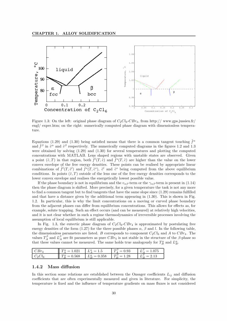
Figure 1.3: On the left: original phase diagram of C2Cl6-CBr4, from http:// www.gps.jussieu.fr/engl/ exper.htm; on the right: numerically computed phase diagram with dimensionless tempera-ture.

Equations (1.29) and (1.30) being satisfied means that there is a common tangent touching f α

and f β in cα and cβ respectively. The numerically computed diagrams in the figures 1.2 and 1.3were obtained by solving (1.29) and (1.30) for several temperatures and plotting the computedconcentrations with MATLAB. Lens shaped regions with unstable states are observed. Givena point (c, T ) in that region, both f l(T, c) and f s(T, c) are higher than the value on the lowerconvex envelope of the free energy densities. These points can be realised by appropriate linearcombinations of f l(T, cl) and f s(T, cs), cl and cs being computed from the above equilibriumconditions. In points (c, T ) outside of the lens one of the free energy densities corresponds to thelower convex envelope and realises the energetically lowest possible value.

If the phase boundary is not in equilibrium and the vαβ -term or the γαβ-term is present in (1.14)then the phase diagram is shifted. More precisely, for a given temperature the task is not any moreto find a common tangent but to find tangents that have the same slope since (1.29) remains fulfilledand that have a distance given by the additional term appearing in (1.30). This is shown in Fig.1.2. In particular, this is why the limit concentrations on a moving or curved phase boundaryfrom the adjacent phases can differ from equilibrium concentrations. This allows for effects as, forexample, solute trapping. Such an effect occurs (and can be measured) at relatively high velocities,and it is not clear whether in such a regime thermodynamics of irreversible processes involving theassumption of local equilibrium is still applicable.

In Fig. 1.3, the eutectic phase diagram of C2Cl6-CBr4 is approximated by postulating freeenergy densities of the form (1.27) for the three possible phases α, β and l. In the following table,the dimensionless parameters are listed. B corresponds to component C2Cl6 and A to CBr4. Thevalues T β

A and LβA are fit parameters as pure CBr4 is not stable in the structure of the β-phase so

that these values cannot be measured. The same holds true analogously for T αB and Lα

B.

CBr4 T αA = 1.021 Lα

A = 1.5 T βA = 0.93 Lβ

A = 1.075

C2Cl6 T αB = 0.568 Lα

B = 0.358 T βB = 1.28 Lβ

B = 2.13

1.4.2 Mass diffusion

In this section some relations are established between the Onsager coefficients Lij and diffusioncoefficients that are often experimentally measured and given in literature. For simplicity, thetemperature is fixed and the influence of temperature gradients on mass fluxes is not considered

30

1.4. CALIBRATION

but only cross effects due to the presence of several components. Since in the present model massdiffusion is a bulk phenomenon (enhanced diffusion in the phase boundaries is not taken into accountbut can easily be involved, cf. [NGS05]) only one phase is considered. The flux (1.5) becomes withT , being fixed, entering the coefficients

Ji =

N∑

i=1

Lij∇(−µj).

According to Fick’s law, diffusion is often modelled by a linear relation between diffusive fluxand concentration gradients (cf. [TAV03], Section 2.4 and the discussion therein). If the diffusivityDik models the influence of gradients of component k on the flux of component i then

Ji = −N∑

k=1

Dik∇ck.

For (1.4) to be fulfilled,

N∑

i=1

Dik = 0, 1 ≤ k ≤ N,

is supposed. Often, one component (w.l.o.g. component N) is considered as solvent for the others

which only appear in a minor concentration. Since cN = 1 − ∑N−1i=1 ci it holds that

Ji = −N∑

k=1

Dik∇ck = −N−1∑

k=1

(Dik − DiN )∇ck =: −N−1∑

k=1

DNik∇ck

with coefficients DNik = Dik −DiN that are often given in literature. In particular, cross effects are

possible in the sense that concentration gradients of one species causes another species to diffuse.An example is the Darken effect [Dar49] for diffusion of carbon in steel under the influence of silicon(cf. again [TAV03], Section 2.4).

Considering µ as a function in c (cf. Appendix B) yields

Ji =

N∑

j=1

Lij∇(−µj) =

N∑

j=1

Lij

N∑

k=1

(−∂ckµj)∇ck = −

N∑

k=1

N∑

j=1

Lij∂ckµj

∇ck

and therefore

Dik =N∑

j=1

Lij∂ckµj or, shortly, D = L∂cµ. (1.31)

In particular,∑

i Dik = 0 is obtained from the corresponding condition on the Lij . In Subsection1.1.1 it is mentioned that L can be chosen to be symmetric. Then D is not symmetric in general.Furthermore,

DNik =

N∑

j=1

Lij(∂ck− ∂cN

)µj .

The fact that L is symmetric imposes constraints on the DNij and on the dependence of the µj on

the concentrations.Instead of using the DN

ik, alternatively to each species an atomic diffusivity or bare mobilityDi(c) can be assigned. Defining

Dik = Di(c)δik − Di(c)ci∑

l Dl(c)clDk(c)

31


it is easy to derive that∑N

i=1 Dik = 0 and, by (1.31),∑N

i=1 Lij = 0. Using cN = 1 − ∑N−1i=1 ci it

holds that

Ji = −N∑

k=1

Dik∇ck

= − Di(c)∇ci +Di(c)ci

∑

l Dl(c)cl

N∑

k=1

Dk(c)∇ck

= − Di(c)∇ci +Di(c)ci

∑

l Dl(c)cl

N−1∑

k=1

(Dk(c) − DN (c))∇ck,

whence there results the following relation to the DNik:

DNik = Di(c)δik − Di(c)ci

∑

l Dl(c)cl(Dk(c) − DN (c)), 1 ≤ i ≤ N, 1 ≤ k ≤ N − 1.

32

Chapter 2

Phase Field Modelling

In this chapter, a general framework based on the phase field approach is presented to describe themicrostructure formation occurring during alloy solidification. In the preceding chapter, an entropyfunctional played a central role involving bulk and surface contributions. Introducing phase fieldvariables and replacing the surface terms by a Ginzburg-Landau type entropy, the motion of the(diffuse) phase boundaries or, respectively, the evolution of the phase fields can be defined by agradient flow of the entropy which yields a set of partial differential equations of parabolic type(see Section 2.1). As before, the evolution is coupled to bulk equations balancing the conservedquantities energy and mass. In particular, a small length scale is involved related to the thicknessof the interfacial layers.

To take kinetic anisotropy of the phase boundaries into account, a deviation from the gradientflow structure is allowed by introducing a positive mobility function depending on the phase fieldsand their gradients. In spite of this deviation, an entropy inequality can be derived again (seeSection 2.2).

To clarify the generality of the developed framework, it is shown in Section 2.3 that, by ap-propriate calibration, i.e., choosing free energies for the phases and suitable potentials for theGinzburg-Landau part of the entropy as well as Onsager coefficients for the fluxes, the governingequations of models are obtained which have been used earlier. More precisely, the models of Cagi-nalp [Cag89] (various asymptotic limits are discussed in this paper), Penrose-Fife [PF90] (in thiswork, thermodynamic consistency is discussed), and Wheeler-Boettinger-McFadden [WMB92] (ason of the first phase field models for an alloy) are derived.

The general framework is formulated in terms of the phase fields and the conserved quantities.Instead of the latter the thermodynamic potentials, namely, the negative inverse temperature andgeneralised chemical potential differences divided by the temperature, may be used. Since thesepotentials are continuous across the phase boundaries in the related sharp interface model, theasymptotic analysis in the following chapter is simplified. The use of the thermodynamic potentialsinstead of the conserved quantities is also motivated by the discussion in [KKS99]. There it wasfound that, when taking the concentration as variable, in the diffuse interfacial region an extraamount of free energy appears which is due to the interpolation properties in the concentration andthe phase field variable. It plays no role in the sharp interface limit since it scales proportional tothe small length scale related to the interface thickness. But if one is interested in a quantitativedescription of a specific alloy and in numerical simulations with, necessarily, relatively high interfacethicknesses then, depending on the material, it is possible that this extra potential cannot be ignoredany more. By using the chemical potential as a variable instead of the concentration, the additionalpotential is avoided.

A good thermodynamic quantity to reformulate the diffusion equations is the reduced grandcanonical potential, defined to be the Legendre transform of the negative entropy with respect tothe conserved quantities energy and concentrations. After its introduction and an example, the

33

CHAPTER 2. PHASE FIELD MODELLING

reformulated general phase field model is presented in Section 2.4.As in the previous chapter, derivatives sometimes are denoted by subscripts after a comma. For

example, s,φ(c, φ) is the derivative of the function s = s(c, φ) in a point (c, φ) with respect to thevariables corresponding to φ.

2.1 The general phase field model

A system with M possible phases and N components is considered. The entropy (1.10) is replacedby an entropy functional of the form

S(c, φ) =

∫

Ω

(

s(c, φ) −(εa(φ,∇φ) +

1

εw(φ)

))

dx. (2.1)

The vector φ = (φα)Mα=1 consists of phase field variables. Each variable φα describes the local

fraction of the corresponding phase α. They are required to fulfil the constraint

φ ∈ ΣM (2.2)

analogously to the constraint (1.2) imposed on the concentrations. Here,

c := (e, c1, . . . cN ) ∈ R × ΣN (2.3a)

denotes the vector of all conserved variables including the internal energy e = c0. The pureconcentration vector is denoted by

c := (c1, . . . , cN ) ∈ ΣN . (2.3b)

The bulk entropy contribution s(c, φ) will later be motivated (see (2.13)). The interfacial con-tribution in (1.10), namely

−M∑

α<β, α,β=1

∫

Γαβ

γαβ(ναβ) dHd−1, (2.4)

is replaced by a Ginzburg-Landau type functional (cf. [LG50]) of the form

−∫

Ω

(

εa(φ,∇φ) +1

εw(φ)

)

dx. (2.5)

The function a : ΣM × (TΣM )d → R is a gradient energy density which is assumed to be smooth,non-negative, and homogeneous of degree two in the second variable, i.e.,

a(φ, X) ≥ 0 and a(φ, ηX) = η2a(φ, X) ∀(φ, X) ∈ ΣM × (TΣM )d and ∀η ∈ R+, (2.6a)

and w : ΣM → R is a smooth function with exactly M global minima at the points eβ = (δαβ)Mα=1,

1 ≤ β ≤ M , with w(eβ) = 0, i.e.,

w(φ) ≥ 0, and w(φ) = 0 ⇔ φ = eβ for some β ∈ 1, . . . , M. (2.6b)

Observe that the eβ are the corners of the set ΣM onto which φ maps by (2.2). Possible choices fora and w are given in Section 2.3.

For the case of two phases it is shown in [Mod87] under appropriate assumptions on a that thefunctional (2.5) Γ-converges to the perimeter functional (2.4) when ε converges to zero. This resultwas generalised to more general surface energies (cf. [AB98]) which motivates the replacement. Itshould be remarked that the rigorous treatment of the case of several order parameters is still anopen problem because of the appearance of triple points or lines, and so far only formal resultsexist (see the following chapter).

34

2.1. THE GENERAL PHASE FIELD MODEL

The evolution of the system is determined by a gradient flow of the entropy for the phase fieldvariables coupled to balance equations for the conserved variables. As shown in the following sectionthe coupling is such that an entropy inequality holds, and the second law of thermodynamics isfulfilled.

To compute the variational derivative of the entropy with respect to the phase field variableslet v : Ω → TΣM be a smooth test function and φ : Ω → int(ΣM ) be smooth where int(ΣM ) isthe interior of ΣM with respect to the induced topology on HΣM from R

M . Observe that thenS(c, φ + δv) is well-defined for δ small enough.

⟨δS

δφ(c, φ), v

⟩

=d

dδ

∫

Ω

(

s(c, φ + δv) −(εa(φ + δv,∇φ + δ∇v) +

1

εw(φ + δv)

))

dx∣∣∣δ=0

=

∫

Ω

M∑

α=1

(

s,φα(c, φ)vα − εa,φα

(φ,∇φ)vα − εa,∇φα(φ,∇φ) · ∇vα − 1

εw,φα

(φ)vα

)

dx

=

∫

Ω

M∑

α=1

(

ε∇ · a,∇φα(φ,∇φ) − εa,φα

(φ,∇φ) − 1

εw,φα

(φ) + s,φα(c, φ)

)

vα dx.

To obtain the last identity the boundary conditions

a,∇φα(φ,∇φ) · νext = 0, 1 ≤ α ≤ M, (2.7)

were imposed.To allow for anisotropy in the mobility of the phase boundaries, analogously as in Definition 1.5

in Subsection 1.1.3 the L2 product is weighted. Given a smooth field φ : Ω → ΣM let

(w, v)ω,φ :=

∫

Ω

ε ω(φ,∇φ)w · v dx ∀w, v ∈ C∞(Ω; TΣM ). (2.8a)

The function ω is supposed to be smooth, positive, and homogeneous of degree zero in the secondvariable, i.e.,

ω(φ, X) ≥ 0 and ω(φ, ηX) = ω(φ, X) ∀(φ, X) ∈ ΣM × Rd×M and ∀η ∈ R

+. (2.8b)

The evolution is of the system, defined by

(∂tφ, v)ω,φ =⟨δS

δφ(c, φ), v

⟩

∀v ∈ C∞(Ω, TΣM ), (2.9)

yields for all test function v : Ω → TΣM

∫

Ω

ε ω(φ,∇φ)∂tφ · v dx

=

∫

Ω

(

ε∇ · a,∇φ(φ,∇φ) − εa,φ(φ,∇φ) − 1

εw,φ(φ) + s,φ(c, φ)

)

· v dx. (2.10)

Observe that since the weight ω of the L2 product depends on φ this is no gradient flow of theentropy as in the sharp interface model. If v : Ω → R

M is an arbitrary test function, then v −PMvmaps onto TΣM , PM being the projection defined in (1.1c). Inserting v − PMv and using

∫

Ω

ξ · (v − PMv) dx =

∫

Ω

(ξ − PMξ) · v dx

for another test function ξ : Ω → RM which holds thanks to the symmetry of PM = 1

M 1M ⊗ 1M

gives for the left hand side of (2.10)∫

Ω

εω(φ,∇φ)∂tφ · (v − PMv) dx =

∫

Ω

εω(φ,∇φ)∂tφ · v dx

35


since ∂tφ(t, x) ∈ TΣM implying PM∂tφ = 0. The right hand side of (2.10) becomes when insertingthe function v − PMv

∫

Ω

∑

α

(


(φ,∇φ) − 1

εw,φα

(φ) + s,φα(c, φ) − λ

)

vα dx

where the Lagrange factor λ is given by

λ =1

M1M ·

(

ε∇ · a,∇φ(φ,∇φ) − εa,φ(φ,∇φ) − 1

εw,φ(φ) + s,φ(c, φ)

)

=1

M

M∑

α=1

(


(φ,∇φ) − 1

εw,φα

(φ) + s,φα(c, φ)

)

. (2.11)

Finally, (2.9) yields

ε ω(φ,∇φ)∂tφ = ε∇ · a,∇φ(φ,∇φ) − εa,φ(φ,∇φ) − 1

εw,φ(φ) + s,φ(c, φ) − λ1M .

The balance equations for the conserved quantities read

∂tci = −∇ · Ji(c, φ,∇u(c, φ)), 0 ≤ i ≤ N,

with the fluxes

Ji(c, φ,∇u(c, φ)) =N∑

j=0

Lij(c, φ)∇(−uj(c, φ)).

Similarly as done in Subsection 1.1.1 it can be shown that this is a gradient flow of the entropywith respect to a weighted H−1-product. The different phases are taken into account by lettingthe potentials and the coefficients depend on the smooth phase field variables. This may be doneas follows:

The free energy of the system can be defined as an appropriate interpolation of the free energiesfα(T, c)α of the possible phases, i.e.

f(T, c, φ) =

M∑

α=1

fα(T, c)h(φα) (2.12)

with an interpolation function h : [0, 1] → [0, 1] satisfying h(0) = 0 and h(1) = 1. By s = −f,T ande = f + Ts = f − Tf,T (see Appendix B) the internal energy can be expressed as a function in(T, c, φ). By appropriate assumptions on f the temperature inversely can be expressed as a functionin (e, c, φ) = (c, φ). Let

Φ : R+ × int(ΣN ) × int(ΣM ) → R × int(ΣN ) × int(ΣM ), (T, c, φ) 7→ (e(T, c, φ), c, φ)

be this change of variables. Using µ = f,c (see Appendix B) and again e = f − Tf,T yields

e,T = −Tf,TT , e,c = µ − Tµ,T , e,φ = f,φ − Tf,Tφ.

Then DΦ(T, c, φ) : R × TΣN × TΣM → R × TΣN × TΣM is given by

DΦ(T, c, φ) =

−Tf,TT µ − Tµ,T f,φ − Tf,Tφ

0 IdTΣN 00 0 IdTΣM

where IdTΣK is the identity on TΣK . Assuming that Tf,TT 6= 0 the inverse function theoremimplies

D(Φ−1)(e, c, φ) =−1

Tf,TT

1 −(µ − Tµ,T ) −(f,φ − Tf,Tφ)0 −Tf,TT IdTΣN 00 0 −Tf,TT IdTΣM

36

2.1. THE GENERAL PHASE FIELD MODEL

where f and its derivatives are evaluated at (T (e, c, φ), c, φ). In the first line the derivatives of Twith respect to e, c and φ can be found. Considering the entropy density as a function in the newvariables (e, c, φ) = (c, φ), i.e.

s(e, c, φ) = −f,T (T (e, c, φ), c, φ), (2.13)

the derivatives of s with respect to (c, φ) can be computed:

s,c0(c, φ) = s,e(e, c, φ) = −f,TT T,e = −f,TT−1

Tf,TT=

1

T= −u0,

s,c(c, φ) = s,c(e, c, φ) = −f,T c − f,TT T,c = −µ,T − f,TT

µ − Tµ,T

Tf,TT=

−µ

T=: −u,

s,φ(c, φ) = s,φ(e, c, φ) = −f,Tφ − f,TT T,φ = −f,Tφ − f,TTf,φ − Tf,Tφ

Tf,TT= −f,φ

T.

The identity in the last line can be inserted into (2.10) and the following equations. Moreoveru0 = −1

T and u = µT are expressed in terms of (c, φ).

The coefficients Lij and the diffusivities (see Subsection 1.4.2) can distinguish in the differentphases, too. This may be modelled by interpolating the coefficients Lα

ijα of the pure phases

analogously as done for the free energy. The matrix L(c, φ) = (Lij(c, φ))Ni,j=0 remains symmetric.

From (1.6a) and (1.6b) the conditions

L = (Lij(c, φ))Ni,j=0 is positive semi-definite, (2.14a)

N∑

i=1

Lij(c, φ) = 0 ∀j ∈ 1, . . . , N (2.14b)

can be deduced. Altogether, the above computations motivate the following definition of the model:

2.1 Definition The evolution of the system is governed by the partial differential equations

∂tci = −∇ · Ji(c, φ,∇u(c, φ)) = ∇ ·(

N∑

j=0

Lij(c, φ)∇uj(c, φ)

)

, (2.15a)

ε ω(φ,∇φ) ∂tφα = ε∇ · a,∇φα(φ,∇φ) − εa,φα

(φ,∇φ) − 1

εw,φα

(φ) − f,φα(T (c, φ), c, φ)

T (c, φ)− λ (2.15b)

where 0 ≤ i ≤ N and 1 ≤ α ≤ M with λ given by

λ =1

M

M∑

α=1

(


(φ,∇φ) − 1

εw,φα

(φ) − f,φα(T (c, φ), c, φ)

T (c, φ)

)

. (2.15c)

The differential equations are subject to initial conditions

c(t = 0) = cic, φ(t = 0) = φic (2.15d)

and boundary conditions

Ji(c, φ,∇u(c, φ)) · νext = 0, 1 ≤ i ≤ N, (2.15e)

a,∇φα(φ,∇φ) · νext = 0, 1 ≤ α ≤ M. (2.15f)

If not otherwise stated, additionally the boundary condition

J0(c, φ,∇u(c, φ)) · νext = 0 (2.15g)

is imposed.

2.2 Remark The boundary condition (2.15e) implies that the system is closed as there is no massflux across the external boundary. If (2.15g) holds true there is no energy flux across the externalboundary and the system is adiabatic. Instead of (2.15g) one may impose different conditions that,for example, correspond to Dirichlet conditions for the temperature. Such boundary conditionscan, for example, model the cooling of the system to a certain temperature.

37


2.2 Non-negativity of entropy production

Analogously as done in Section 1.3, it is shown in the following that the equations in Definition 2.1governing the evolution imply a locally non-negative entropy production which is the second lawof thermodynamics. The calculation is much easier than in Section 1.3 as no jumps of fields acrossphase boundaries are involved but only smooth fields appear.

The time derivative of the integrand of the entropy (2.1) is

∂t

(

s(c, φ) − εa(φ,∇φ) − 1

εw(φ)

)

= s,c · ∂tc︸︷︷︸

I

+ s,φ · ∂tφ − ε(a,φ · ∂tφ + a,∇φ : ∇∂tφ) − 1

εw,φ · ∂tφ

︸︷︷︸

II

.

Using (2.15a) and s,c = −u yields for I (the dependence of the functions on c and φ is omitted hereand in the following for a shorter presentation)

I =

N∑

i=0

ui∇ ·

N∑

j=0

Lij∇(−uj)

= ∇ ·

N∑

i,j=0

uiLij∇(−uj)

−N∑

i,j=0

∇ui · Lij∇(−uj)

= ∇ ·(

N∑

i=0

uiJi

)

+

N∑

i,j=0

∇(−ui) · Lij∇(−uj).

Using (2.15b) it holds for the second term that

II =

M∑

α=1

(

s,φα∂tφα − εa,φα

∂tφα − εa,∇φα· ∇(∂tφα) − 1

εw,φα

∂tφα

)

=M∑

α=1

(

−f,φα

T− εa,φα

+ ε∇ · a,∇φα− 1

εw,φα

)

∂tφα −M∑

α=1

ε∇ · (a,∇φα∂tφα)

= ε ω(φ,∇φ)

M∑

α=1

(∂tφα)2+

∑

α

λ∂tφα

︸︷︷︸

=λ∂t

P

φα=0

−ε

M∑

α=1

∇ · (a,∇φα∂tφα) .

Integrating I and II with respect to the space gives, using the divergence theorem,

∂tS(c, φ) =

∫

Ω

(I + II) dx

=

∫

Ω

N∑

i,j=0

∇(−ui) · Lij∇(−uj) + ε ω(φ,∇φ)M∑

α=1

(∂tφα

)2

dx (2.16a)

−∫

∂Ω

(N∑

i=0

(−ui)Ji + ε(a,∇φα

∂tφα

)

)

· νext dHd−1. (2.16b)

From (2.16a) and using Assumptions (2.14a) and (2.8b) it is clear that the local entropy productionis non-negative,

N∑

i,j=0

∇(−ui) · Lij∇(−uj) + ε ω(φ,∇φ)ε

M∑

α=1

(∂tφα

)2 ≥ 0.

38

2.3. EXAMPLES

Moreover, (2.16b) implies that the entropy flux

Js :=

N∑

i=0

(−ui)Ji + ε

M∑

α=1

a,∇φα∂tφα

consists of two terms. The first one is due to energy and mass diffusion and the second one due tomoving phase boundaries (cf. [AP92]). With the boundary conditions (2.15e), (2.15g), and (2.7) itholds that

∂tS(c, φ) ≥ 0

which is the desired entropy inequality for an isolated system.

2.3 Examples

The phase field model from Definition 2.1 generalises earlier models that have successfully beenapplied to describe such phenomena as mentioned in the Introduction. In the next subsectionsthis is exemplarily shown for the models used in [Cag89, PF90, WMB92] by postulating suitablefunctions a, w, and f .

2.3.1 Possible choices of the surface terms

First, some examples for the terms modelling interfacial contributions to the entropy are given.The simplest form of the gradient energy is

a(φ,∇φ) = γ|∇φ|2 = γM∑

α=1

|∇φα|2

or, more generally,

a(φ,∇φ) =∑

α<β

gαβ∇φα · ∇φβ (2.17a)

with constants γ and gαβ , α, β ∈ 1, . . . , M. However, as shown in [SPN+96, GNS99a], gradientenergies of the form

a(φ,∇φ) =∑

α<β

Aαβ(φα∇φβ − φβ∇φα), (2.17b)

where the Aαβ are convex functions that are homogeneous of degree two, are more convenient withrespect to the calibration of parameters in the phase field model to the surface terms in the sharpinterface model. A choice that leads to isotropic surface terms is

a(φ,∇φ) =∑

α<β

γαβ

mαβ|φα∇φβ − φβ∇φα|2

with constants γαβ and mαβ that can be related to γαβ and mαβ (cf. [GNS98]).Possible choices for the mobility function (2.8b) are given and discussed in [GNS99b, NGS05].

A general form is

ω(φ,∇φ) = ω0 +∑

α<β

Bαβ(φα∇φβ − φβ∇φα)

39


where the Bαβ are smooth functions that are homogeneous of degree zero and that can be relatedto the mobility coefficient mαβ(ν) of the α-β-phase transition (see the following chapter).

For the bulk potential one may take the standard multi-well potential

wst(φ) = 9∑

α<β

mαβ γαβφ2αφ2

β (2.18)

or a higher order variant

wst(φ) = wst(φ) +∑

α<β<δ

γαβδφ2αφ2

βφ2δ.

For numerical computations, the obstacle potential with multiple wells yields good calibrationproperties. It is defined by

wob(φ) =

16π2

∑

α<β mαβ γαβφαφβ if φ ∈ ΣM ,

∞ elsewhere,

with a higher order variant

wob(φ) =

wob(φ) +∑

α<β<δ γαβδφαφβφδ if φ ∈ ΣM ,

∞ elsewhere.

The calibration properties of the presented multi-well potentials are discussed in [GNS99b] and[GHS05].

2.3.2 Relation to the Penrose-Fife model

Now, it is demonstrated that the general model includes the model of Penrose and Fife [PF90] asa special case. There is only one component, and the variable c can be neglected. There are twophases, a solid one an a liquid one, hence the equations can be written down in terms of the solidfraction ϕ = φ1. Then, by (2.2), φ2 = 1 − ϕ. Moreover, instead of using the density of the internalenergy as variable, the temperature is taken.

The first phase, the solid one, is characterised by φ = e1 of, equivalently, ϕ = 1. Its free energydensity is postulated to be

fs(T ) = LT − Tm

Tm− cvT (ln(T ) − 1),

where Tm is the melting temperature and L the latent heat of the solid-liquid phase transition. Thesecond phase, the liquid one, is characterised by φ = e2 ⇔ ϕ = 0, and its free energy density ispostulated to be

f l(T ) = −cvT (ln(T ) − 1).

Setting

f(T, ϕ, 1 − ϕ) = LT − Tm

Tmh(ϕ) − cvT (ln(T ) − 1) (2.19)

it holds that s(T, ϕ, 1 − ϕ) = − LTm

h(ϕ) + cv ln(T ) and

e(T, ϕ, 1 − ϕ) = −Lh(ϕ) + cvT.

40

2.3. EXAMPLES

The evolution equation (2.15a) for the energy yields

cv∂tT − Lh′(ϕ)∂tϕ = −∇ ·(

L00∇1

T

)

.

Choosing L00 = cvK2T2 the right hand side becomes cvK2∆T .

Furthermore, the simple gradient entropy term

a(φ,∇φ) =γ

2|∇φ|2 =

γ

2(|∇φ1|2 + |∇φ2|2) = γ|∇ϕ|2

where γ = κ1cv

ε for some constant κ1 is taken. Then a,∇φα= γ∇φα, ∇ · a,∇φα

= γ∆φα anda,φα

= 0. Inserting this into the phase field equations (2.15b) yields

εω∂tφ1 = εγ∆φ1 −1

εw,φ1 −

1

Tf,φ1 − λ, (2.20a)

εω∂tφ2 = εγ∆φ2 −1

εw,φ2 −

1

Tf,φ2 − λ (2.20b)

with

λ =1

2

(

εγ∆φ1 −1

εw,φ1 −

1

Tf,φ1 + εγ∆φ2 −

1

εw,φ2 −

1

Tf,φ2

)

.

Since ϕ = φ1 = 1 − φ2 it holds that ∂tφ1 = ∂tϕ, ∂tφ2 = −∂tϕ, ∆φ1 = ∆ϕ and ∆φ2 = −∆ϕ.Moreover,

w,φ1(ϕ, 1 − ϕ) − w,φ2(ϕ, 1 − ϕ) = ∂ϕw(ϕ, 1 − ϕ),

f,φ1(T, ϕ, 1 − ϕ) − f,φ2(T, ϕ, 1 − ϕ) = ∂ϕf(T, ϕ, 1 − ϕ).

Subtracting (2.20b) from (2.20a) gives

2εω∂tϕ = 2εγ∆ϕ − 1

ε∂ϕw(ϕ, 1 − ϕ) − 1

T∂ϕf(T, ϕ, 1 − ϕ). (2.21)

By (2.19), − 1T ∂ϕf(T, ϕ, 1 − ϕ) = L( 1

T − 1Tm

)h′(ϕ). Setting ω ≡ 12ε , K1 = cv

2ε and defining

s0(ϕ) := − 1

εcvw(ϕ, 1 − ϕ) − L

cvTmh(ϕ), λ(ϕ) := Lh′(ϕ)/cv

the equations (2.21) and (2.15a) become

∂tϕ = K1

(λ(ϕ)

T+ s′0(ϕ) + κ1∆ϕ

)

,

∂tT − λ(ϕ)∂tϕ = K2∆T

which is the model in [PF90], Chapter 6.

2.3.3 A linearised model

In this subsection the general model is partially linearised. This is done in such a way that theevolution equations in the pure phases are linear, i.e., they reduce to standard linear diffusionequations. Only a binary system is considered, but a generalisation to multi-component systems isstraightforward.

By c = c1 the concentration of the first component is denoted, hence c2 = 1 − c. The fact thatL is symmetric and the algebraic constraints (2.14b) give

L01 = L10 = −L02 = −L20 and L11 = L22 = −L12 = −L21.

41


Setting f (T, c) = f(T, c, 1 − c) gives as in Subsection 1.4.1

f,c = µ1 − µ2.

Therefore Li1∇(−µ1)+ Li2∇(−µ2) = Li1∇f,c , i = 0, 1, 2, and the conservation laws for energy andconcentration read

∂te = −∇ · L00∇1

T−∇ · L10∇

−f,cT

, (2.22a)

∂tc = −∇ · L10∇1

T−∇ · L11∇

−f,cT

. (2.22b)

Defining e(T, c) := f (T, c) − T f,T (T, c) and choosing

L11 = DT

f,cc, L10 = L01 = e,cD

T

f,cc, and L00 = e2

,cDT

f,cc+ KT 2,

the equations (2.22a) and (2.22b) become after a short calculation

∂te = ∇ ·(

K∇T + e,cD∇c + e,cDf,cφ

f,cc∇φ

)

, (2.22c)

∂tc = ∇ ·(

D∇c + Df,cφ

f,cc∇φ

)

. (2.22d)

The diffusivity coefficients K and D may depend on φ. It remains to couple equations (2.22c) and(2.22d) to the equations for the phase field variables (2.15b).

If the internal energy density is affine linear in the variables (T, c), i.e.,

e(T, c) = cvT + e,cc with e,c constant,

then the system (2.22c)–(2.22d) reduces in regions where φ is constant, i.e., in the pure phases(where, the diffusivities K and D are constants), to

cv∂tT = ∇ · K∇T = K∆T, ∂tc = ∇ · D∇c = D∆c.

These are classical linear diffusion equations for temperature (Fourier’s law) and concentration(Fick’s law).

2.3.4 Relation to the Caginalp model

Further linearisation of the model leads to a generalisation of the original phase field model [Cag89]to the case of alloy solidification. Let M = 3, N = 2 (a three-phase system for a binary alloy isconsidered) and choose the free energy density

f (T, c, φ) =(

κc

2−

3∑

α=1

Lα1 φα

)

cT − cvT(

ln( T

Tref

)− 1

)

−3∑

α=1

Lα2 φα,

where Lα2 are latent heat coefficients and Lα

1 and κ, respectively, are coefficients entering thechemical potentials. As in the preceding subsection, c = c1 and c2 = 1 − c1 = 1 − c. Then

s = −f,T = −(

κc

2−

3∑

α=1

Lα1 φα

)

c + cv ln( T

Tref

),

e = f + Ts = cvT −∑

α

Lα2 φα,

µ1 − µ2

T=

f,cT

= κc −∑

α

Lα1 φα,

f,φα

T= −Lα

1 c − Lα2

T.

42

2.3. EXAMPLES

The mobility matrix is chosen as in the previous subsection leading to

∂te = ∂t

(

cvT −∑

α

Lα2 φα

)

= ∇ · (K∇T ),

∂tc = ∇ · D∇(

κc −∑

α

Lα1 φα

)

.

For the gradient energy the isotropic function a(φ,∇φ) = γ2

∑

α |∇φα|2 is taken as in Subsection2.3.2. Then the equations for the phase field variables are of the form

ωε∂tφα = εγ∆φα − 1

εw,φα

(φ) + Lα1 c +

Lα2

T− λ,

The term 1T can be linearised around a reference temperature Tm: so that

ωε∂tφα = εγ∆φα − 1

εw,φα

(φ) + Lα1 c + Lα

2

(1

Tm− 1

T 2m

(T − Tm)

)

− λ.

The equations for (T, c) are linear, and all terms in the equation for φ are linear except the termw,φα

.It should be remarked that the above choice of the free energy density leads to a linearised

phase diagram. In particular, the magnitude of the jump of the concentration in the sharp interfacemodel is constant for each of the phase boundaries (cf. equations (1.29) and (1.30) in Subsection1.4.1).

2.3.5 Relation to the Warren-McFadden-Boettinger model

In the model used in [WMB92] double-well potentials are used with coefficients depending on theconcentration. The presented general model is not intended for a concentration dependence of w.But it turns out that, if the constants WA and WB in equations (8) and (9) of [WMB92] are equal(let WA = WB =: W ), then the concentration dependence of the double-well potential drops out.the following derivation it restricted to the latter case.

A binary alloy involving two phases is considered. Diffusion of heat is supposed to be muchfaster than the relaxation of the phase boundaries and the mass diffusion. Therefore the energyequation is not considered and a constant temperature is assumed. The variables ϕ = φ1 andc = c1 introduced in the Subsection 2.3.2 and 2.3.3 are used again. Component 1 corresponds tocomponent B in [WMB92]. As in Subsection 2.3.2, the gradient entropy term

a(φ,∇φ) =K

2|∇φ|2

leads to the phase field equation

2εω∂tϕ = 2εK∆ϕ − 1

ε∂ϕw(ϕ, 1 − ϕ) − 1

T∂ϕf (c, ϕ, 1 − ϕ).

Setting ω = 1M1

and K = δ2 this becomes

∂tϕ = M1

(

δ2∆ϕ − 1

2ε2∂ϕw(ϕ, 1 − ϕ) − 1

2εT∂ϕ f (c, ϕ, 1 − ϕ)

)

.

If the multi-well potential

w(φ1, φ2) =ε2W

2φ2

1φ22

is chosen then 12ε2 ∂ϕw(ϕ, 1−ϕ) = W w ′(ϕ) with w(ϕ) = 1

4ϕ2(1−ϕ)2, and the phase field equationreads

∂tϕ = M1

(

δ2∆ϕ − W w ′(ϕ) − 1

2εT∂ϕ f (c, ϕ, 1 − ϕ)

)

.

43


The free energy density is postulated to be

f (c, ϕ, 1 − ϕ) =εW

3

(cβB(T ) + (1 − c)βA(T )

)Th(ϕ) +

2R

vmT

(c ln(c) + (1 − c) ln(1 − c)

)

where h(ϕ) = (3−2ϕ)ϕ2 and the functions βB(T ) and βA(T ) are explained in [WMB92] just belowequation (7). Then

1

2εT∂ϕ f (c, ϕ, 1 − ϕ) =

W

6

(cβB(T ) + (1 − c)βA(T )

)h′(ϕ)

and hence the phase field equation reads

∂tϕ = M1

(

δ2∆ϕ − W w ′(ϕ) − W

6

(cβB(T ) + (1 − c)βA(T )

)h′(ϕ)

)

which is equation (17) from [WMB92] (for the case WA = WB = W ). Since

f,cφ1(c, ϕ, 1 − ϕ) =W

3

(βB(T ) − βA(T )

)Th′(ϕ),

f,cφ2(c, ϕ, 1 − ϕ) = 0,

f,cc(c, ϕ, 1 − ϕ) =2R

vm

T

c(1 − c),

and choosing L11 = D Tf,cc

as in Subsection 2.3.3, (2.22d) becomes

∂tc = ∇ ·(

D∇c + Dvm

R

c(1 − c)

2

W

3

(βB(T ) − βA(T )

)Th′(ϕ)∇ϕ

)

= D∆c + M2∇ ·(

c(1 − c)∇(W

6

(βB(T ) − βA(T )

)h(ϕ)

))

with M2 = Dvm

R which is equation (18) from [WMB92]. Since the equations (17) and (18) governthe evolution in [WMB92] it is shown that their model can be recovered by the presented generalone under the mentioned condition WA = WB .

2.4 The reduced grand canonical potential

2.4.1 Motivation and introduction

In Subsection 1.4.1 the relation between free energies and phase diagrams is established. Thefollowing chapters motivate that, sometimes, the reduced grand canonical potential is more appro-priate for the analysis. The entropy is a function in the conserved variables internal energy andconcentrations (cf. (B.4) in Appendix B) and the reduced grand canonical potential is defined tobe the Legendre transform (cf. [ET99]) of the negative entropy. Some structural assumptions onthe entropy are necessary. As usual let

e := c0, c := (c0, c1, . . . , cN ) Ã s = s(c).

Let int(ΣN ) be the interior of ΣN with respect to the induced topology on HΣN ⊂ RN and

assume that

R1 (−s) : C := E × int(ΣN ) → R with an open interval E ⊂ R is smooth and strictly convex,

R2 ∇(−s) : C → U is a C∞-diffeomorphism into a convex open set U ⊂ R × TΣN .

44

2.4. THE REDUCED GRAND CANONICAL POTENTIAL

In Assumption R2, the tangent space TcC on C in c ∈ C is identified with R × TΣN according toDefinition 1.1. Observe that E×int(ΣN ) is a convex subset of an affine linear subspace. AssumptionR1 implies that D2(−s)(c), acting on (R × TΣN )2, is positive and has full rank so that, locally,Assumption R2 is already satisfied.

In the following, the sets C and U are considered as subsets of RN+1, and c · u is the standard

scalar product on RN+1 for elements c ∈ C and u ∈ U .

2.3 Lemma With the Assumptions R1 and R2 the Legendre transform of the entropy density

(−s)∗(u) := supc∈C

c · u + s(c), u ∈ U,

is a real valued smooth function (−s)∗ : U → R. Besides

∇(−s)∗(u) = c.

Proof: For given u, c = c(u) := (∇(−s))−1(u) exists by Assumption R2. From the convexityof s in Assumption R1 it follows that this is the only critical point of c 7→ c · u + s(c) and that thisis the global maximum. Hence (−s)∗(u) = c(u) ·u + s(c(u)). The identity for the derivative followseasily using ∇(−s)(c) = u. ¤

2.4 Definition If the entropy density s satisfies the Assumptions R1 and R2 then the density ofthe reduced grand canonical potential is defined by

ψ : U → R, ψ(u) = (−s)∗(u).

Analogously as in [ET99] it can be shown that

(−s)∗∗ = ψ∗ = −s. (2.23)

Besides the preceding computations motivate to write

ψ = c · u + s, dψ = c · du = edu0 +N∑

i=1

cidui. (2.24)

A relation to the grand canonical potential b (see (B.5) in Appendix B) can be derived as follows:

ψ = s + u · c = s +−1

T(e −

N∑

i=1

µici)

= s +−1

T(f + sT −

N∑

i=1

µici) =−1

T(f − µici)

=1

Tb = −u0b. (2.25)

Using that (B.8) is equivalent to (1.13b) and (1.14) for a fixed temperature the equilibriumconditions on a phase boundary between two phases α and β transform into

uα = uβ, ψα = ψβ . (2.26)

45


2.4.2 Example

For a binary alloy with components A and B the free energy density

f(T, c1, c2) = LAT − TA

TAc1 + LB

T − TB

TB+ RT (c1 ln(c1) + c2 ln(c2)) − cvT

(

ln(T

Tref) − 1

)

is postulated (cf. (1.27)). Then

s = −f,T = −(LA

TAc1 +

LB

TBc2

)

− R(c1 ln(c1) + c2 ln(c2)) + cv ln(T

Tref).

Moreover

e = f + Ts = −LAc1 − LBc2 + cvT,

and, hence, the temperature can be written as a function in (e, c1, c2):

T =1

cv(e + LAc1 + LBc2).

Then also −s can be written as a function in c = (e, c1, c2)

−s(c) =(LA

TAc1 +

LB

TBc2

)

+ R(c1 ln(c1) + c2 ln(c2)) − cv ln( 1

cvTref(e + LAc1 + LBc2)

)

.

Since u = ∇c(−s)(c) ∈ R × TΣ2 it is obvious that u0 = ∇c(−s)(c) · (1, 0, 0)⊥. Moreover u1 = −u2,hence 2u1 = u1 − u2 = ∇c(−s)(c) · (0, 1,−1)⊥. The above function for −s(c) yields

u0 = − cv

e + LAc1 + LBc2,

2u1 = LA

( 1

TA− cv

e + LAc1 + LBc2

)

− LB

( 1

TB− cv

e + LAc1 + LBc2

)

+ R ln(c1

c2).

Using c2 = 1 − c1 the above functions can be inverted, and c can be written as a function in u. Ashort calculation yields

e(u) = − cv

u0− LA

1

1 + ev1(u)− LB

1

1 + ev2(u),

c1(u) =1

1 + ev1(u),

c2(u) =1

1 + ev2(u)

where

v1(u) =1

R

(

LA(u0 − uA) − LB(u0 − uB) − 2u1

)

,

v2(u) =1

R

(

LB(u0 − uB) − LA(u0 − uA) − 2u2

)

= −v1(u)

with uA := −1TA

and uB := −1TB

. The entropy density becomes

s(c(u)) =( LAuA

1 + ev1(u)+

LBuB

1 + ev2(u)

)

+ R( ln(1 + ev1(u))

1 + ev1(u)+

ln(1 + ev2(u))

1 + ev2(u)

)

− cv ln(−u0Tref).

46

2.4. THE REDUCED GRAND CANONICAL POTENTIAL

Figure 2.1: Reduced grand canonical potential ψ from the example in Subsection 2.4.2 as a functionin u0 and u1 = −u2. The parameters are given in (2.27).

Inserting this and c(u) into (2.24) gives the reduced grand canonical potential density

ψ(u) = c(u) · u + s(c(u))

= −cv − LAu0

1 + ev1(u)− LBu0

1 + ev2(u)+

u1

1 + ev1(u)+

u2

1 + ev2(u)

+( LAuA

1 + ev1(u)+

LBuB

1 + ev2(u)

)

+ R( ln(1 + ev1(u))

1 + ev1(u)+

ln(1 + ev2(u))

1 + ev2(u)

)

− cv ln(−u0Tref )

=(LA(uA − u0)

1 + ev1(u)+

LB(uB − u0)

1 + ev2(u)

)

+(u1 + R ln(1 + ev1(u))

1 + ev1(u)+

u2 + R ln(1 + ev2(u))

1 + ev2(u)

)

− cv

(1 + ln(−u0Tref )

).

Fig. 2.1 shows this potential for the following values:

LA = 1.0, LB = 1.2, uA = 0.8, uB = 1.4, R = 1.0, cv = 1.0, Tref = 1.0. (2.27)

Up to the last term, the growth in u is nearly linear while the last term tends to infinity as u0 0.

2.4.3 Reformulation of the model

The aim is now to write down the equations governing the evolution in terms of (u, φ) insteadof (c, φ). For this purpose, the density of the reduced grand canonical potential ψ including itsderivatives is used.

In the preceding section it is shown how the reduced grand canonical potential density of aphase can be computed given the free energy density of the phase. In a multi-phase system thereare therefore densities ψα : Uα → R, 1 ≤ α ≤ M , for the possible phases with Uα ⊂ R × TΣN

defined in Assumption R2 in Section 2.4. Assume that U =⋂M

α=1 Uα is non-empty. The functionψ : U × ΣM → R is obtained as a suitable interpolation of the ψα such that ψ(u, eα) = ψα(u), forexample (see also the Remark 2.6 below)

ψ : U × ΣM → R, ψ(u, φ) =

M∑

α=1

ψα(u)h(φα) (2.28)

with an interpolation function

h : [0, 1] → [0, 1] satisfying h(0) = 0, h(1) = 1. (2.29)

47


It is assumed that the Legendre transformation in Lemma 2.3 as well as the backward transfor-mation (2.23) is possible after adapting the domains Uφ and Cφ in dependence of φ. Let φ ∈ ΣM

be fixed. Given ψ, sufficient conditions for the backward transformation to obtain s read similarlyas the Assumptions R1 and R2 in Section 2.4 for the forward transformation. Hence

s(c, φ) = ψ(u(c, φ), φ) − c · u(c, φ) (2.30a)

where

c = ∇uψ(u, φ) = (∇uψ(·, φ))(u) ⇔ u = (∇ψ(·, φ))−1(c). (2.30b)

If the dependence of ψ on φ is smooth then also the domains Uφ and Cφ depend smoothly onφ in the following sense: Given u ∈ Uφ and c = ψ,u(u, φ) ∈ Cφ there is a small ball Bκ(φ) ⊂ ΣM of

radius κ around φ such that u ∈ Uφ and c ∈ Cφ for all φ ∈ Bκ(φ). Thus, varying φ is possible in(2.30a) which with (2.30b) provides the identity

s,φ(c, φ) · v =

M∑

α=1

(

u,φα· ψ,u(u, φ)︸︷︷︸

=c

+ψ,φα(u, φ) − u,φα

· c)

vα = ψ,φ(u, φ) · v (2.31)

for every v ∈ TΣM . Using this, the identity s,φ = − f,φ

T , and (2.30b), the model in Definition 2.1can be reformulated considering (u, φ) as variables:

2.5 Definition The evolution of the system is governed by the partial differential equations

∂tψ,ui(u, φ) = −∇ · Ji(ψ,u(u, φ), φ,∇u) = ∇ ·

(N∑

j=0

Lij(ψ,u(u, φ), φ)∇uj

)

, (2.32a)

ε ω(φ,∇φ)∂tφα = ε∇ · a,∇φα(φ,∇φ) − εa,φα

(φ,∇φ) − 1

εw,φα

(φ) + ψ,φα(u, φ) − λ (2.32b)


λ =1

M

M∑

α=1

(


(φ,∇φ) − 1

εw,φα

(φ) + ψ,φα(u, φ)

)

. (2.32c)

The differential equations are subject to initial conditions

u(t = 0) = uic, φ(t = 0) = φic (2.32d)


Ji(ψ,u(u, φ), φ,∇u) · νext = 0, 1 ≤ i ≤ N, (2.32e)

a,∇φα(φ,∇φ) · νext = 0, 1 ≤ α ≤ M. (2.32f)

If not otherwise stated, additionally the boundary condition

J0(ψ,u(u, φ), φ, ) · νext = 0 (2.32g)

is imposed.

2.6 Remark Of course it is possible to choose interpolation functions in (2.28) involving u. Indeed,instead of interpolating the densities of the reduced grand canonical potentials, first, the free energydensities could be interpolated similarly to (2.12), and after the procedure as in the example of theprevious section could be carried out to gain ψ from f . It turns out that, for the limiting modelas ε → 0, it does not matter which interpolation is chosen. But in numerical simulations morecomplicated interpolations involve more computational effort and, since in applications feasiblevalues for ε have to be chosen (the smaller ε the higher the costs), different results may be obtained.

48

Chapter 3

Asymptotic Analysis

This chapter is dedicated to the limit of the general phase field model as ε → 0. It is demonstratedthat the relation between the phase field model presented in Subsection 2.4.3 and the sharp interfacemodel presented in Section 1.2 can be established using the method of matched asymptotic expan-sions. For this purpose, methods developed in [CF88, BGS98, GNC00, GNS98] are generalised. Itis supposed that, in the bulk regions of the pure phases as well as in the interfacial regions, thesolution to the phase field model can be expanded in ε-series. In Section 3.1 necessary conditionsare derived for that these expansions match. It turns out that the coefficient functions to leadingorder of the ε expansions in the bulk regions exactly fulfil the governing equations of the sharpinterface model (see Section 3.2).

It should be remarked that this procedure is a formal method in the sense that it is not rigorouslyshown that the assumed expansions in fact exist or converge respectively. But in some cases, thisansatz could be verified (cf. [ABC94, CC98, MS95, Sto96]).

In the following Section 3.3 the quality of the approximation of the sharp interface is of interest.The approximation obtained in Section 3.2 is of first order in the small parameter ε. For example,expanding the temperature in the pure phases in the form T = T0 + εT1 + O(ε2) the asymptoticanalysis yields that T0 satisfies the equations of the sharp interface problem. But if T1 vanishes theapproximation of T0 is of second order in ε. To see whether this is possible, the asymptotic analysishas to be continued in order to derive the equations T1 has to fulfil which leads to the notion of anO(ε)-correction problem.

An improvement of the approximation was obtained in [KR98] in the context of a thin interfaceasymptotic analysis. The analysis led to a positive correction term in the kinetic coefficient ofthe phase field equation balancing undesirable O(ε)-terms in the Gibbs-Thomson condition andraising the stability bound of explicit numerical methods. Besides, the better approximation allowsfor larger values of ε and, therefore, for coarser grids. In particular, it is possible to consider thelimit of vanishing kinetic undercooling which is important in applications. Numerical simulations ofappropriate test problems reveal an enormous gain in efficiency thanks to a better approximation.

In [Alm99] the analysis was extended to the case of different diffusivities in the phases andboth classical and thin interface asymptotics were discussed. By choosing different interpolationfunctions for the free energy density and the internal energy density an approximation of secondorder could still be achieved but the gradient structure of the model and thermodynamic consistencywere lost. In [And02] it was shown, based on [Alm99], that even an approximation of third order ispossible by using high order polynomials for the interpolation. McFadden, Wheeler, and Anderson[MWA00] used an approach based on an energy and an entropy functional providing more degreesof freedom to tackle the difficulties with unequal diffusivities in the phases while avoiding the loss ofthe thermodynamic consistency. Both classical and thin asymptotics hare discussed in the paper aswell as the limit of vanishing kinetic undercooling. In a more recent analysis in [RBKD04], a binaryalloy also involving different diffusivities in the phases was considered and a better approximation

49

CHAPTER 3. ASYMPTOTIC ANALYSIS

was obtained by adding a small additional term to the mass flux (anti-trapping mass current, theideas stem from [Kar01]).

In the present work it is shown that, for two phase multi-component systems with arbitraryphase diagrams, there is a correction term to the kinetic coefficient such that the model with movingboundaries is approximated to second order. A new feature compared to the existing results is that,in general, this correction term depends on u, i.e., on temperature and chemical potentials. Indeed,up to some numerical constants, the latent heat appears in the correction term obtained by Karmaand Rappel [KR98]. Analogously, the equilibrium jump in the concentrations enters the correctionterm when investigating an isothermal binary alloy. But from realistic phase diagrams it is obviousthat this jump depends on the temperature leading to a temperature dependent correction term inthe non-isothermal case.

To investigate the gain in efficiency thanks to the better approximation results of numericalsimulations to the phase field model with and without correction term are compared in Section 3.4.

For the derivations, some assumptions on the occurring functions are necessary:

A1 The core of the matrix L = (Lij)Ni,j=0 of Onsager coefficients is the space orthogonal to

R × TΣN (cf. assumption L2 in Subsection 1.1.1), i.e.,

ker(L) = span(0, 1, . . . , 1) ⊂ RN+1 = (Y N )⊥

where

Y N = R × TΣN .

Then, for each v ∈ Y N , there is a unique solution ξ ∈ Y N of the equation Lξ = v. Thesolution is denoted by L−1v.

A2 In addition to (2.29), the interpolation functions fulfils

h′(0) = h′(1) = 0.

A3 Around its minima eβ , 1 ≤ β ≤ M , the function w is strictly convex. This means that

w,φφ(eβ) > 0, 1 ≤ β ≤ M.

This chapter only treats the two dimensional case (i.e., d = 2). The generalisation to the threedimensional case is straightforward. The differentials along curves simply become surface gradientsor surface divergences.

Several times the homogeneity of a is used. This is why the following facts are stated at thebeginning of this chapter: It holds that

a,φ(φ, η∇φ) = η2a,φ(φ,∇φ), a,∇φ(φ, η∇φ) = ηa,∇φ(φ,∇φ), (3.1a)

and, moreover,

a(φ, 0) = 0, a,φ(φ, 0) = 0, a,∇φ(φ, 0) = 0, a,∇φ(φ,∇φ) : ∇φ = 2a(φ,∇φ) (3.1b)

for all φ ∈ ΣM , ∇φ ∈ (TΣM )d, and η > 0.

50

3.1. EXPANSIONS AND MATCHING CONDITIONS

3.1 Expansions and matching conditions

The matching procedure for asymptotic expansions in the context of phase field models is outlinedwith great care in [FP95]. Here, only the main ideas are sketched.

Consider a time interval I = (0, tend) and an interfacial region in a domain D ⊂ R2 where two

phases meet. The family of curves Γ(t; ε)ε>0, t∈I is supposed to be a set of smooth curves in Dwhich are uniformly bounded away from ∂D and depend smoothly on (ε, t) such that, if ε → 0, somesmooth limiting curve Γ(t; 0) is obtained. By Dl(t; ε) and Ds(t; ε) the regions occupied by the twophases are denoted. The limiting curve Γ(t; 0) corresponds to the sharp interface between the phasesin the sense of Section 1.2, i.e., to some curve of a phase boundary Γsl, while the approximatingcurves Γ(t; ε) are given somehow as level sets of the phase field variables. In the model of Definition2.1 in Section 2.1, for example, if (φ(t, x; ε), c(t, x; ε)) is the solution of (2.15a)–(2.15g), then Γ(t; ε)may be defined by

Γ(t; ε) :=

x ∈ D : φl(t, x; ε) = φs(t, x; ε)

, ε > 0, t ∈ I. (3.2)

Let γ(t, s; 0) be a parametrisation of Γ(t; 0) by arc-length s ∈ [0, l(t)] for every t ∈ I, l(t) beingthe length of Γ(t; 0). The vector ν(t, s; 0) denotes the unit normal on Γ(t; 0) pointing into Dl(t; 0),and the vector τ(t, s; 0) := ∂sγ(t, s; 0) denotes the unit tangent vector towards the parametrisation.The orientation is such that (ν, τ) is positively oriented.

Using some distance function d(t, s; ε), the curves Γ(t; ε) can be parametrised over Γ(t; 0) by

γ(t, s; ε) := γ(t, s; 0) + d(t, s; ε)ν(t, s; 0). (3.3)

Close to ε = 0 it is assumed that there is the expansion d(t, s; ε) = d0(t, s)+ ε1d1(t, s)+ ε2d2(t, s)+O(ε3). Since d(t, s; 0) ≡ 0 the expansion becomes

d(t, s; ε) = ε1d1(t, s) + ε2d2(t, s) + O(ε3). (3.4)

Near Γ(t; 0), the coordinates (s, r) are well-defined, r being the signed distance of x from Γ(t; 0)(positive towards ν, i.e., if x ∈ Dl(t; 0)). Let z = r

ε and ε0 > 0. For each t ∈ I and ε ∈ (0, ε0) thereare the diffeomorphisms

Fε(t, s, z) := (t, γ(t, s; 0) + (εz + d(t, s; ε))ν(t, s))

mapping an open set V (t; ε) ⊂ R2 onto an open tube B(t) around Γ(t; 0). The coordinates (t, s, z)

are such that the curve Γ(t; ε) is given by the set Fε(t, s, z)|z = 0. It is supposed that, uniformlyin t and ε, the tube B(t) is large enough such that values for z lying in a fixed interval aroundzero are allowed as arguments for z. To obtain expressions for ∇(t,x)z(t, x) and ∇(t,x)s(t, x) it isnecessary to compute the inverse of the derivative of Fε.

Let κ := κ(t, s; 0) be the curvature of Γ(t; 0) defined by ∂sτ = κν or, equivalently, by ∂sν = −κτ .Furthermore let

v = v(t, s; 0) = ∂tγ(t, s; 0) · ν(t, s; 0) (normal velocity, intrinsic), (3.5a)

vτ = vτ (t, s; 0) = ∂tγ(t, s; 0) · τ(t, s; 0) (tangential velocity, non-intrinsic). (3.5b)

Hence, writing dε = d(t, s; ε),

DFε(t, s, z) =

(∂tt(t, s, z) ∂st(t, s, z) ∂zt(t, s, z)∂tx(t, s, z) ∂sx(t, s, z) ∂zx(t, s, z)

)

=

(1 0 0

∂tγ + (εz + dε)∂tν + (∂tdε)ν τ − (εz + dε)κτ + (∂sdε)ν εν

)

51


and, using (3.5a) and (3.5b),

D(F−1ε )(t, x) = (DFε)

−1(t, x) =

∂tt(t, x) ∇xt(t, x)∂ts(t, x) ∇xs(t, x)∂tz(t, x) ∇xz(t, x)

=

1 (0, 0)− 1

1−κ(εz+dε)(vτ + (εz + dε)τ · ∂tν) 11−κ(εz+dε)τ

T

1ε

(

−∂tdε + ∂sdε(εz+dε)1−κ(εz+dε) τ · ∂tν + ∂sdε

1−κ(εz+dε)vτ − v)

1ενT − ∂sdε

ε(1−κ(εz+dε))τT

with ∂tγ, ∂tν, ν, τ , κ, vτ and v evaluated at (t, s; 0). The ansatz (3.4) yields the expansion

1

1 − κ(εz + dε)= 1 + εκ(z + d1) + ε2

(κd2 + κ2(z + d1)

2)

+ O(ε3),

whence

∂ts(t, x) = −vτ + O(ε),

∇xs(t, x) =(

1 + εκ(z + d1) + ε2(κd2 + κ2(z + d1)

2)

+ O(ε3))

τ,

∂tz(t, x) = − 1εv − (∂td1 − ∂sd1vτ ) + O(ε),

∇xz(t, x) = 1εν −

(

∂sd1 + ε(∂sd2 + ∂sd1κ(z + d1)

))

τ

−ε2(

∂sd3 + ∂sd2κ(z + d1) + ∂sd1κd2 + ∂sd1κ2(z + d1)

2)

τ + O(ε3).

A short calculation shows that for a function B(t, s, z) and for a vector field ~B(t, s, z) it holds that

ddtB = − 1

εv∂zB + ∂B − (∂d1)∂zB + O(ε), (3.6a)

∇xB = 1ε∂zB ν + (∂sB − ∂sd1∂zB) τ

+ε(κ(z + d1)∂sB − (∂sd2 + ∂sd1κ(z + d1))∂zB

)τ + O(ε2), (3.6b)

∇x · ~B = 1ε∂z

~B · ν + (∂s~B − ∂sd1∂z

~B) · τ+ε

(κ(z + d1)∂s

~B − (∂sd2 + ∂sd1κ(z + d1))∂z~B)· τ + O(ε2), (3.6c)

∆xB = 1ε2 ∂zzB − 1

εκ∂zB

+(∂sd1)2∂zzB − 2∂sd1∂szB − κ2(z + d1)∂zB − ∂ssd1∂zB + ∂ssB + O(ε) (3.6d)

where ∂ = ∂t − vτ∂s is the (intrinsic) normal-time-derivative (see Appendix C). This identityis motivated by the following calculation: Consider a field f(t, x) in I × D and write f (t, s) =f(t, γ(t, s)) for f restricted on Γ(t; 0). Then it holds with (C.1)

∂t f (t, s) − vτ∂s f (t, s)

=d

dtf(t, γ(t, s)) − ∂tγ(t, s) · τ(t, s)∂sf(t, γ(t, s))

= ∂tf(t, γ(t, s)) + ∂tγ(t, s) · ∇xf(t, γ(t, s)) − ∂tγ(t, s) · τ(t, s)∇xf(t, γ(t, s)) · τ(t, s)

= ∂tf(t, γ(t, s)) +((

∂tγ(t, s) · ν(t, s))ν(t, s) +

(∂tγ(t, s) · τ(t, s)

)τ(t, s)

)

· ∇xf(t, γ(t, s))

− (∂tγ(t, s) · τ(t, s))τ(t, s) · ∇xf(t, γ(t, s))

= ∂tf(t, γ(t, s)) + v(t, s)ν(t, s) · ∇xf(t, γ(t, s))

= ∂(1,(vν)(t,s))f(t, γ(t, s))

= ∂f(t, γ(t, s)).

52

3.1. EXPANSIONS AND MATCHING CONDITIONS

Now assume that the normal velocity and the curvature of Γ(t; ε) can be expanded in ε-series,

v(t, s; ε) = v0(t, s; 0) + εv1(t, s; 0) + ε2v2(t, s; 0) + . . . ,

κ(t, s; ε) = κ0(t, s; 0) + εκ1(t, s; 0) + ε2κ2(t, s; 0) + . . . .

The first order corrections v1 and κ1 can be written in terms of d1:

3.1 Lemma It holds that

κ(t, s; ε) = κ(t, s; 0) + ε(κ(t, s; 0)2d1(t, s) + ∂ssd1(t, s)

)+ O(ε2), (3.7a)

v(t, s; ε) = v(t, s; 0) + ε∂d1(t, s) + O(ε2). (3.7b)

Proof: The unit tangent vector and the unit normal vector are

τ(t, s; ε) =∂sγε

|∂sγε|=

(1 − κdε)τ + (∂sdε)ν

((1 − κdε)2 + (∂sdε)2)1/2,

ν(t, s; ε) =∂sγ

⊥ε

|∂sγε|=

(1 − κdε)ν − (∂sdε)τ

((1 − κdε)2 + (∂sdε)2)1/2

where ∂sγ⊥ε is the rotation of ∂sγε by 90 degree such that (∂sγ

⊥ε , ∂sγε) is positively oriented.

Inserting the expansion (3.4) yields

(

(1 − κdε)2 + (∂sdε)

2)−1/2

= 1 + εκd1(t, s) + O(ε2)

and for v(t, s; ε) the expansion

v(t, s; ε) = ∂tγε · ν(t, s; ε)

=(∂tγ(t, s; 0) + ∂tdεν + dε∂tν) · ((1 − κdε)ν − (∂sdε)τ)

((1 − κdε)2 + (∂sdε)2)1/2

=(1 − κdε)v + ∂tdε(1 − κdε) − ∂sdεvτ − dε∂sdε∂tν · τ

((1 − κdε)2 + (∂sdε)2)1/2

= v + ε∂d1 + O(ε2)

where ∂tν · ν = 12∂t|ν|2 = 0 was used. To compute the expansion of κ(t, s; ε), the identity

∂ssγ(t, s; ε) = −(

2(∂sdε)κ + dε(∂sκ))

τ +(

κ + ∂ssdε − κ2dε

)

ν

implies

det(∂sγ(t, s; ε), ∂ssγ(t, s; ε)) = −(1 − κdε)(κ + ∂ssdε − κ2dε) − (∂sdε)(2(∂sdε)κ + dε(∂sκ)),

and with

|∂sγε|−3 = (1 − 2κdε + κ2d2ε + (∂sd

2ε))

−3/2 = 1 + ε 3κd1 + O(ε2)

this gives

κ(t, s; ε) =− det(∂sγε, ∂ssγε)

|∂sγε|3= κ + ε

(

κ2d1 + ∂ssd1

)

+ O(ε2).

¤

Consider some function b(t, x) (in the next subsections, b corresponds to φ, c or u). Supposethat, in each domain D ⊂⊂ D\Γ(t; 0), the function b can be expanded in a series close to ε = 0(outer expansion): For some K ≥ 2

b(t, x; ε) =

K∑

k=0

εkb(k)(t, x) + O(εK+1). (3.8)

53


Hence, in a neighbourhood of Γ(t; 0), the functions

b(t, s, r; ε) := b(t, x; ε). (3.9)

are well-defined for r 6= 0. To be more precise, the expansion

b(t, s, r; ε) =

K∑

k=0

εkb(k)(t, s, r) + O(εK+1) (3.10)

is assumed to be valid uniformly on

V αout :=

(t, s, r; ε) : t ∈ I, s ∈ [0, l(t)], r ∈ (εα δ0

2 , δ0], ε ∈ (0, ε0]

for every α ∈ (0, 1). Furthermore it is assumed that function b(k) can be smoothly and uniformlyextended onto Γ(t; 0) from both sides, i.e., as r 0 and r 0 respectively.

Let B(t, s, z; ε) := b(t, s, r; ε) with r = εz. Suppose that the function B can be expanded in aseries as follows (inner expansion):

B(t, s, z; ε) =K∑

k=0

εkB(k)(t, s, z) + O(εK+1). (3.11)

It is assumed that the functions B(k)(t, s, z) are well-defined for t ∈ I, s ∈ [0, l(t)] and z ∈ R, andthat they approximate some polynomial in z uniformly in t, s for large z, i.e.,

B(k)(t, s, z) ≈ B±k,0(t, s) + B±

k,1(t, s)z + B±k,2(t, s)z

2 + · · · + B±k,nk

(t, s)znk , z → ±∞, (3.12)

with nk ∈ N for all k. Moreover, the expansion (3.11) shall be valid uniformly on

V αinn :=

(t, s, z; ε) : t ∈ I, s ∈ [0, l(t)], z ∈ εα−1[−δ0, δ0], ε ∈ (0, ε0]

for every α ∈ (0, 1).

3.2 Definition (cf. [LP88]) Let ζ ∈ ( δ0

2 , δ0), ε ∈ (0, ε0] and α ∈ (0, 1).

1. The variable ζεα is called intermediate variable.

2. The expansions (3.10) and (3.11) are said to match if the following holds:When replacing r in (3.10) and z in (3.11) by an arbitrary intermediate variable, i.e., r = ζεα

and z = r/ε = ζεα−1, then, in the limit as ε → 0, the coefficients agree to every order in εand ζ.

3.3 Lemma For that the two expansions (3.8) and (3.11) of b match in the limit as ε → 0 thefollowing conditions must be fulfilled: As z → ±∞

B(0)(z) ≈ b(0)(0±), (3.13a)

B(1)(z) ≈ b(1)(0±) + (∇b(0)(0±) · ν)z, (3.13b)

∂zB(1)(z) ≈ ∇b(0)(0±) · ν, (3.13c)

∂zB(2)(z) ≈ ∇b(1)(0±) · ν + (ν · D2b(0)(0±)ν)z. (3.13d)

Here, b(0+) denotes the limit of b(t, x) if r(t, x) = dist(x, Γ(t; 0)) → 0 where x ∈ Dl(t; 0) which isequivalent to r 0; analogously, b(0−) is defined considering x ∈ Ds(t; 0) or r 0.

54

3.2. FIRST ORDER ASYMPTOTICS OF THE GENERAL MODEL

Proof: An expansion of the functions b(k) in (3.10) in Taylor series at r = 0 yields

b(k)(t, s, r) = b(k)(t, s, 0+) + ∂r b(k)(t, s, 0+)r + 1

2∂rrb(k)(t, s, 0+)r2 + O(r3), r ∈ (0, δ0], (3.14a)

b(k)(t, s, r) = b(k)(t, s, 0−) + ∂r b(k)(t, s, 0−)r + 1

2∂rrb(k)(t, s, 0−)r2 + O(r3), r ∈ [−δ0, 0). (3.14b)

If r is replaced by an intermediate variable ζεα then, for ε small enough, r = ζεα indeed is small,and the above expansion (3.14a) is valid and gives for (3.10) (dropping the dependence on (t, s))

b(ζεα; ε) = ε0b(0)(0+) + εα∂r b(0)(0+)ζ + ε2α 1

2∂rrb(0)(0+)ζ2 + O(ε3α)

+ ε1b(1)(0+) + ε1+α∂rb(1)(0+)ζ + ε1+2α 1

2∂rr b(1)(0+)ζ2 + O(ε1+3α)

+ ε2b(2)(0+) + ε2+α∂rb(2)(0+)ζ + ε2+2α 1

2∂rr b(2)(0+)ζ2 + O(ε2+3α)

+ O(ε3 + ε4α).

Equation (3.14b) yields the same with 0+ replaced by 0− if −ζ ∈ ( δ0

2 , δ0).The expansion (3.11) is valid for z = ζεα−1. Using (3.12) and again dropping the dependence

on (t, s) gives

B(ζεα−1; ε) = ε0B+0,0 + εα−1B+

0,1ζ + · · · + εn0(α−1)B+0,n0

ζn0

+ ε1B+1,0 + ε1+α−1B+

1,1ζ + · · · + ε1+n1(α−1)B+1,n1

ζn1

+ ε2B+2,0 + ε2+α−1B+

2,1ζ + · · · + ε2+n2(α−1)B+2,n2

ζn2 + . . .

The same holds true for −ζ ∈ ( δ0

2 , δ0) with B+ replaced by B−.

By Definition 3.2 the expansions of B and b are said to match if, in the limit ε → 0, thecoefficients to every order in ε and ζ agree for every α ∈ (0, 1). Comparing the two series yieldsthe following relations between the coefficients B+

k,n on the one hand and the derivatives ∂jru(0+)

on the other hand for k ≤ 2:

B+0,0 = b(0)(0+), B+

0,i = 0, 1 ≤ i ≤ n0,

B+1,0 = b(1)(0+), B+

1,1 = ∂r b(0)(0+), B+

1,i = 0, 2 ≤ i ≤ n1,

B+2,0 = b(2)(0+), B+

2,1 = ∂r b(1)(0+), B+

2,2 = 12∂rrb

(0)(0+), B+2,i = 0, 3 ≤ i ≤ n2.

It is obvious from the definition of r and (3.9) that a derivative of b with respect to r corresponds

to the derivative of b with respect to x towards ν = ν(t, s(t, x); 0). Hence, ∂r b(k) = ∇xb(k) · ν and,

since ν is independent of r, ∂rrb(k) = ν ·D2

xb(k)ν. Using (3.12) again yields the following matchingconditions corresponding to (3.13a)–(3.13d): As z → +∞

B(0)(z) ≈ b(0)(0+),

B(1)(z) ≈ b(1)(0+) + (∇b(0)(0+) · ν)z,

∂zB(1)(z) ≈ ∇b(0)(0+) · ν,

∂zB(2)(z) ≈ ∇b(1)(0+) · ν + (ν · D2b(0)(0+)ν)z.

Analogously, the result for 0− can be shown. ¤

3.2 First order asymptotics of the general model

The goal of this section is to figure out the limit of the general phase field system (2.32a), (2.32b),(2.32e)–(2.32g) as ε → 0, i.e., the limit of the equations

ε ω(φ,∇φ)∂tφ = PM

(

ε∇ · a,∇φ(φ,∇φ) − εa,φ(φ,∇φ) − 1

εw,φ(φ) + ψ,φ(u, φ)

)

, (3.15a)

∂tc(u, φ) = −∇ · J(c(u, φ), φ,∇u) = ∇ · (L(c(u, φ), φ)∇u) , (3.15b)

55


subject to the boundary conditions

Ji(c(u, φ), φ,∇u) · νext = 0, 0 ≤ i ≤ N, (3.15c)

a,∇φα(φ,∇φ) · νext = 0, 1 ≤ α ≤ M. (3.15d)

For this purpose, the method of matched asymptotic expansions is used. Expansions of the variablesu and φ of the form (3.8) and (3.11) are plugged into the governing equations and matched accordingto the conditions in Lemma 3.3.

3.4 Theorem Let u(t, x; ε), φ(t, x; ε)ε denote a family of solutions to the system (3.15a)–(3.15d).Consider phase boundaries Γαβ , α < β, α, β ∈ 1, . . . , M, and assume that the solutions can beexpanded according to (3.8) in the adjacent bulk regions. Then the coefficient function u(0) andthe motion of the phase boundaries Γαβ satisfy the following equations:

In the bulk regions Ωα, α ∈ 1, . . . , M, the balance equations

∂tcαi (u(0)) = −∇ · Jα

i (c(u(0)),∇u(0)) = ∇ ·(

N∑

j=0

Lαij(c

α(u(0)))∇u(0)j

)

, 0 ≤ i ≤ N, (3.16a)

are fulfilled. On the phase boundaries Γαβ it holds that

[u(0)i ]βα = 0, 0 ≤ i ≤ N, (3.16b)

[ci(u(0))]βαvαβ = [Ji(c(u

(0)),∇u(0))]βα · ναβ , 0 ≤ i ≤ N, (3.16c)

mαβ(ναβ)vαβ = −∇Γ · ∇γαβ(ναβ) + [ψ(u(0))]βα. (3.16d)

There is no flux across the external boundary,

Jαi (c(u(0)),∇u(0)) · νext = 0 on ∂Ωα, 0 ≤ i ≤ N, 1 ≤ α ≤ M, (3.16e)

and the angle conditions (1.24g) and (1.24h) are satisfied.

Proof: The equations are derived in the following subsections, namely (3.16a) and (3.16e) in3.2.1, (3.16b) and (3.16c) in 3.2.3, and (3.16d) in 3.2.4. The angle conditions (1.24g) and (1.24h)can be derived as in [GNS98].

3.2.1 Outer solution

Based on experiences from numerical simulations it is known that, when solving the equations ofDefinition 2.5, several phases arise which are separated by diffuse interfaces with a thickness of orderε. In such a phase, away from an interface to another phase, an outer expansion is considered. Anansatz according to (3.8) is made:

u(t, x; ε) =

K∑

k=0

εku(k)(t, x) + O(εK+1), φ(t, x) =

K∑

k=0

εkφ(k)(t, x) + O(εK+1), (3.17)

where, for the constraints φ ∈ ΣM and u ∈ Y N to be satisfied,

φ(0) ∈ HΣM , φ(k) ∈ TΣM , k ≥ 1,

u(k) ∈ Y N , k ≥ 0.

The components of the vectors are denoted by u(k)j , 0 ≤ j ≤ N , and φ

(k)α , 1 ≤ α ≤ M , respectively.

First the equation (3.15a) for the phase field variables is considered. Expanding PMw,φ(φ) gives

PMw,φ(φ) = PMw,φ(φ(0)) + ε(PMw,φ),φ(φ(0)) · φ(1) + O(ε2).

56


To leading order O(ε−1) equation (3.15a) becomes

0 = PMw,φ(φ(0)) = w,φ(φ(0)) − 1

M

(M∑

α=1

w,φα(φ(0))

)

1. (3.18)

If a is expanded analogously to w in (φ(0),∇φ(0)) then the boundary conditions (3.15d) become toleading order O(ε0)

0 = a,∇φ(φ(0),∇φ(0)) · νext. (3.19)

Since only stable solutions are of interest, φ(0) is constant (here, the homogeneity of a resulting in(3.1b) is used for the boundary conditions) and one of the minima of w, i.e., in view of (2.6b) oneof the base vectors eβ1≤β≤M . This means that the whole domain Ω is partitioned into phases toleading order which are characterised by the M possible values of φ(0).

To the next order O(ε0) equation (3.15a) becomes

0 = −(PMw,φ),φ(φ(0)) · φ(1) + PMψ,φ(u(0), φ(0)). (3.20)

Inserting φ(0) = eβ for some β ∈ 1, . . . , M gives w,φφ(φ(0)) > 0 due to assumption A3. Moreover,by (2.28) and assumption A2 it holds that ψ,φ(u(0), φ(0)) = 0. Hence, the only solution to (3.20) isφ(1) = 0. This solution is consistent with the boundary conditions for φ(1) resulting from equation(3.15d) to order O(ε1) which reads

0 =(

(a,∇φ),φ(φ(0),∇φ(0)) · φ(1) + (a,∇φ),∇φ(φ(0),∇φ(0)) : ∇φ(1))

· νext. (3.21)

The O(ε0)-equations for the conserved variables are

∂tci(u(0), φ(0)) = ∇ ·

N∑

j=0

Lij(c(u(0), φ(0)), φ(0))∇u

(0)j , 0 ≤ i ≤ N. (3.22)

It should be noted that the fields ci(u(0), φ(0)) and the coefficients Lij were expanded analogously

to PMw,φ. Boundary conditions at the external boundary result from (3.15c) which is to orderO(ε0):

Ji(c(u(0), φ(0)), φ(0),∇u(0)) · νext = 0, 0 ≤ i ≤ N. (3.23)

In the following subsections, boundary conditions on the moving phase boundaries between thephases are derived by matching with inner expansions of the variables in interfacial regions.

In phase α, the equations (1.24c) and (1.24i) are obtained by inserting φ(0) = eα into (3.22)which gives

∂tci(u(0), eα) = ∇ ·

N∑

j=0

Lij(c(u(0), eα), eα)∇u

(0)j , 0 ≤ i ≤ N,

and into (3.23) which yields

Ji(c(u(0), eα), eα,∇u(0)) · νext = 0, 0 ≤ i ≤ N.

3.2.2 Inner expansion

Now, an interfacial region is considered where, without loss of generality, φ(0) = e1 in one of theadjacent phases, denoted by Ω1, and φ(0) = e2 in the other one, denoted by Ω2. These two phasesare supposed to be separated by a family Γ(t; ε)ε>0, t∈I of evolving smooth curves defined as in(3.2) with φl replaced by φ1 and φs by φ2.

57


In the interfacial region, the functions u and φ are expanded according to (3.11):

u(t, x; ε) =

K∑

k=0

εkU (k)(t, s, z) + O(εK+1), φ(t, x; ε) =

K∑

k=0

εkΦ(k)(t, s, z) + O(εK+1), (3.24)

where

Φ(0) ∈ ΣM , Φ(k) ∈ TΣM , k ≥ 1,

U (k) ∈ Y N , k ≥ 0,

to ensure that the constraints on φ and u are satisfied. Taking a Taylor expansion of ci and Lij

around (U (0), Φ(0)) and writing L0,inij = Lij(c(U

(0), Φ(0)), Φ(0)), the conservation laws for mass and

energy give to lowest order O(ε−2)

0 = ν · d

dz

N∑

j=0

L0,inij ∂zU

(0)j ν

=d

dz

N∑

j=0

L0,inij ∂zU

(0)j

, 0 ≤ i ≤ N, (3.25)

where ∂zν = 0 was used. Integrating with respect to z over R yields

L0,in∂zU(0) = k (3.26)

for some vector k ∈ RN+1.

The O(ε−1)-equations of the conserved quantities (3.15b) are with (3.6a)–(3.6c) and ∂sν = −κτ

−v∂zci(U(0), Φ(0)) = τ ·

( d

ds− ∂sd1

d

dz

)

N∑

j=0

L0,inij ∂zU

(0)j ν

+ ν · d

dz

N∑

j=0

L0,inij

(

∂zU(1)j ν + (∂s − ∂sd1∂z)U

(0)j τ

+ ν · d

dz

N∑

j=0

(

terms involving derivatives of Lij

)

∂zU(0)j ν

= −κ

N∑

j=0

L0,inij ∂zU

(0)j

+d

dz

N∑

j=0

L0,inij ∂zU

(1)j

(3.27)

+d

dz

N∑

j=0

(

terms involving derivatives of Lij

)

∂zU(0)j

.

Considering the equations for the phase field variables, similarly as done in [GNS98], the a-termsare expanded in (Φ(0), ∂zΦ

(0) ⊗ ν). Using (3.6b) and (3.6c) the expansions

PMa,φ(φ,∇φ) =1

ε2PMa,φ(Φ(0), ∂zΦ

(0) ⊗ ν)

+1

ε(PMa,φ),φ(Φ(0), ∂zΦ

(0) ⊗ ν) · Φ(1)

+1

ε(PMa,φ),∇φ(Φ(0), ∂zΦ

(0) ⊗ ν) : ((∂s − ∂sd1∂z)Φ(0) ⊗ τ + ∂zΦ

(1) ⊗ ν)

+ O(ε0)

58


and

PM (∇ · a,∇φ(φ,∇φ)) = ∇ · (PMa,∇φ(φ,∇φ))

=1

ε2

d

dz

(

PMa,∇φ(Φ(0), ∂zΦ(0) ⊗ ν)

)

ν

+1

ε

d

dz

(

(PMa,∇φ),φ(Φ(0), ∂zΦ(0) ⊗ ν) · Φ(1)

)

ν

+1

ε

d

dz

(

(PMa,∇φ),∇φ : ((∂s − ∂sd1∂z)Φ(0) ⊗ τ + ∂zΦ

(1) ⊗ ν))

ν

+1

ε

( d

ds− ∂sd1

d

dz

)(

PMa,∇φ(Φ(0), ∂zΦ(0) ⊗ ν)

)

τ

+ O(ε0)

hold. The w-term is expanded in Φ(0) and the ψ-term in (U (0), Φ(0)).To leading order O(ε−1) equation (3.15a) reads

0 =d

dz

(

PMa,∇φ(Φ(0), ∂zΦ(0) ⊗ ν)

)

ν − PMa,φ(Φ(0), ∂zΦ(0) ⊗ ν) − PMw,φ(Φ(0)). (3.28)

Multiplying this equation with ∂zΦ(0) ∈ TΣM gives (the projection PM can be dropped)

0 =d

dz

(

a,∇φ(Φ(0), ∂zΦ(0) ⊗ ν)

)

: (∂zΦ(0) ⊗ ν)

− a,φ(Φ(0), ∂zΦ(0) ⊗ ν) · ∂zΦ

(0) − w,φ(Φ(0)) · ∂zΦ(0)

=d

dz

(

a,∇φ(Φ(0), ∂zΦ(0) ⊗ ν) : (∂zΦ

(0) ⊗ ν))

− a,∇φ(Φ(0), ∂zΦ(0) ⊗ ν) : (∂zzΦ

(0) ⊗ ν)

− a,φ(Φ(0), ∂zΦ(0) ⊗ ν) · ∂zΦ

(0) − d

dz

(

w(Φ(0)))

=d

dz

(

a,∇φ(Φ(0), ∂zΦ(0) ⊗ ν) : (∂zΦ

(0) ⊗ ν) − a(Φ(0), ∂zΦ(0) ⊗ ν) − w(Φ(0))

)

. (3.29)

The equation to order O(ε0) is with (3.6a)

−ω(Φ(0), ∂zΦ(0) ⊗ ν)v∂zΦ

(0) =d

dz

(

(PMa,∇φ),φ · Φ(1) + (PMa,∇φ),∇φ : (∂zΦ(1) ⊗ ν)

)

ν

+d

dz

(

(PMa,∇φ),∇φ : ((∂s − ∂sd1∂z)Φ(0) ⊗ τ)

)

ν

− (PMa,φ),φ · Φ(1) − (PMa,φ),∇φ : (∂zΦ(1) ⊗ ν)

− (PMa,φ),∇φ : ((∂s − ∂sd1∂z)Φ(0) ⊗ τ)

+( d

ds− ∂sd1

d

dz

)(

PMa,∇φ

)

τ

− (PMw,φ),φ · Φ(1) + PMψ,φ(U (0), Φ(0)), (3.30)

where w and all its derivatives are evaluated at Φ(0) and a and its derivatives in (Φ(0), ∂zΦ(0) ⊗ ν).

3.2.3 Jump and continuity conditions

Throughout this subsection, for u(0) in the outer expansions (3.17) in the phases Ω1 and Ω2 thesuperscripts u(0),1 and u(0),2 are used.

First the matching conditions are applied to the functions U(0)j , 0 ≤ j ≤ N , solving the differ-

ential equations (3.26). By assumption A1

∂zU(0) = (L0,in)−1k.

59


Thanks to the matching condition (3.13a) the function U (0) must be bounded if |z| → ∞ sinceu(0)(0±) is finite. Hence ∂zU

(0)(z) → 0 as z → ±∞. Since L0,in = L(U (0), Φ(0)) → L(u(0),1, e1) 6= 0as z → ∞ and L0,in → L(u(0),2, e2) 6= 0 as z → −∞, by assumption A1 necessarily k = 0 so thatU (0) is constant. But due to (3.13a) this means that u(0),1(0+) = u(0),2(0−) which is condition(1.24d).

Since ∂zU(0) = 0, the O(ε−1)-equations (3.27) for the conserved variables simplify to

−v∂zci(U(0), Φ(0)) =

d

dz

N∑

j=0

L0,inij ∂zU

(1)j

.

Integrating with respect to z from −∞ to ∞ (or, more precisely, integrating from −R to R andthen considering the limit as R → ∞) and using that v(t, s) is independent of z, yields

v[

ci(U(0), Φ(0))

]z∞

z−∞= −

N∑

j=0

Lij(U(0), Φ(0))∂zU

(1)j

z∞

z−∞

.

The matching condition (3.13a) for φ and u implies on the one hand

v[

ci(U(0), Φ(0))

]z∞

z−∞= v

(ci(u

(0),1, e1) − ci(u(0),2, e2)

)= v

[ci

]1

2.

On the other hand, thanks to the matching condition (3.13c),

−

N∑

j=0

Lij(c(U(0), Φ(0)), Φ(0))∂zU

(1)j

z∞

z−∞

= −( N∑

j=0

Lij(c(u(0),1, e1), e1)∇xu

(0),1j · ν

)

(0+) −( N∑

j=0

Lij(c(u(0),2, e2), e2)∇xu

(0),2j · ν

)

(0−)

=(

Ji(c(u(0),1, e1), e1,∇u(0),1)(0+) − Ji(c(u

(0),2, e2), e2,∇u(0),2)(0−))

· ν

=[Ji

]1

2· ν.

Altogether this is the desired jump condition (1.24e).

3.2.4 Gibbs-Thomson relation and force balance

In the bulk regions Ω1 and Ω2 adjacent to the interfacial region under consideration it holds thatφ(0) = eα, α ∈ 1, 2. Due to (3.13a), for each s ∈ [0, l(t)] equation (3.28) has to be solved subjectto the boundary conditions

Φ(0)(z) → e1 as z → ∞, Φ(0)(z) → e2 as z → −∞. (3.31)

Integrating (3.29) with respect to z and using (3.1b) and w(e1) = w(e2) = 0 the equation

0 = a,∇φ(Φ(0), ∂zΦ(0) ⊗ ν) : (∂zΦ

(0) ⊗ ν) − a(Φ(0), ∂zΦ(0) ⊗ ν) − w(Φ(0)).

is obtained. With the last identity in (3.1b) this implies

a(Φ(0), ∂zΦ(0) ⊗ ν) = w(Φ(0)),

which is known as equipartition of energy. Setting

C0,1αβ ([−1, 1], ΣM) :=

p ∈ C0,1([−1, 1]; ΣM) | p(−1) = eα and p(1) = eβ

,

60


the surface entropy in direction e ∈ Rd is proposed to be

γαβ(e) = inf

2

∫ 1

−1

√

w(p)√

a(p, p′ ⊗ e)(y) dy | p ∈ C0,1αβ

. (3.32)

This representation was introduced in [Ste91] for isotropic surface energies and in [GNS98] for thegeneral case. It is shown that, if a minimiser exists for e = ν(t, s), then a reparametrisation of theminimiser fulfils (3.28) and, in addition,

γ2,1(ν) =

∫ ∞

−∞

(

a(Φ(0), ∂zΦ(0) ⊗ ν) + w(Φ(0))

)

dz. (3.33)

In [BBR05] the Γ-limit of a functional of the form (2.5) was computed. Besides a rigorous represen-tation formula for γαβ(ν) was found from which it is not known whether it coincides with (3.32).For applications and numerical simulations it is therefore strictly necessary to test the calibrationproperties of the chosen potentials a and w.

The goal is now to deduce the Gibbs–Thomson law. First observe that due to the matchingconditions (3.13b) and (3.13c)

∂zΦ(0)(z) → 0, Φ(1)(t, s, z) → 0, ∂zΦ

(1)(t, s, z) → 0 as z → ±∞. (3.34)

The equation (3.28) for Φ(0) is multiplied by ∂zΦ(1) ∈ TΣM and the equation (3.30) for Φ(1) by

∂zΦ(0) ∈ TΣM . Again the projections PM can be dropped. Then the two equations are summed

and integrated from −∞ to ∞ with respect to z. Altogether

∫ ∞

−∞

((3.28) · ∂zΦ

(1) + (3.30) · ∂zΦ(0)

)dz (3.35)

is computed. The terms involving w and its derivatives vanish:

−∫ ∞

−∞((w,φ),φ · Φ(1)) · ∂zΦ

(0) from (3.30)

−∫ ∞

−∞w,φ · ∂zΦ

(1) from (3.28)

= −∫ ∞

−∞((w,φ),φ · ∂zΦ

(0)) · Φ(1) +

∫ ∞

−∞∂z(w,φ) · Φ(1) − [w,φ · Φ(1)]∞−∞

= − [w,φ(Φ(0)) · Φ(1)]∞−∞ = 0,

since by (3.31) w,φ(Φ(0)) → w,φ(e1,2) = 0 and by (3.34) Φ(1) is bounded as z → ±∞ . Concerningthe a-terms, evaluated at (Φ(0), ∂zΦ

(0) ⊗ ν), the contribution from (3.30) to (3.35) is

∫ ∞

−∞∂z

((a,∇φ),φ · Φ(1)

): (∂zΦ

(0) ⊗ ν) dz +

∫ ∞

−∞∂z

((a,∇φ),∇φ : (∂zΦ

(1) ⊗ ν))

: (∂zΦ(0) ⊗ ν) dz

+

∫ ∞

−∞∂z

((a,∇φ),∇φ : ((∂s − ∂sd1∂z)Φ

(0) ⊗ ν))

: (∂zΦ(0) ⊗ ν) dz

−∫ ∞

−∞((a,φ),φ · Φ(1)) · ∂zΦ

(0) dz −∫ ∞

−∞((a,φ),∇φ : (∂zΦ

(1) ⊗ ν)) · ∂zΦ(0) dz

−∫ ∞

−∞((a,φ),∇φ : ((∂s − ∂sd1∂z)Φ

(0) ⊗ τ) · ∂zΦ(0) dz

+

∫ ∞

−∞((∂s − ∂sd1∂z)a,∇φ) : (∂zΦ

(0) ⊗ τ) dz

61


= [((a,∇φ),φ · Φ(1)) : (∂zΦ(0) ⊗ ν)]∞−∞

︸︷︷︸

=:(t1)

−∫ ∞

−∞((a,∇φ),φ · Φ(1)) : (∂zzΦ

(0) ⊗ ν) dz

︸︷︷︸

=:(t2)

+ [((a,∇φ),∇φ : (∂zΦ(1) ⊗ ν)) : (∂zΦ

(0) ⊗ ν)]∞−∞︸︷︷︸

=:(t3)

−∫ ∞

−∞((a,∇φ),∇φ : (∂zΦ

(1) ⊗ ν)) : (∂zzΦ(0) ⊗ ν) dz

︸︷︷︸

=:(t4)

+ [((a,∇φ),∇φ : ((∂s − ∂sd1∂z)Φ(0) ⊗ τ)) : (∂zΦ

(0) ⊗ ν)]∞−∞︸︷︷︸

=:(t5)

−∫ ∞

−∞((a,∇φ),∇φ : ((∂s − ∂sd1∂z)Φ

(0) ⊗ τ)) : (∂zzΦ(0) ⊗ ν) dz

−∫ ∞

−∞((a,φ),φ · Φ(1)) · ∂zΦ

(0) dz

︸︷︷︸

=:(t6)

−∫ ∞

−∞((a,φ),∇φ : (∂zΦ

(1) ⊗ ν)) · ∂zΦ(0) dz

︸︷︷︸

=:(t7)

−∫ ∞

−∞((a,φ),∇φ : ((∂s − ∂sd1∂z)Φ

(0) ⊗ τ) · ∂zΦ(0) dz

+

∫ ∞

−∞((∂s − ∂sd1∂z)a,∇φ) : (∂zΦ

(0) ⊗ τ) dz,

while the contribution from (3.28) to (3.35) is

∫ ∞

−∞(∂za,∇φ) : (∂zΦ

(1) ⊗ ν) dz −∫ ∞

−∞a,φ · ∂zΦ

(1) dz

=

∫ ∞

−∞((a,∇φ),φ · ∂zΦ

(0)) : (∂zΦ(1) ⊗ ν) dz

︸︷︷︸

=(t7)

+

∫ ∞

−∞((a,∇φ),∇φ : (∂zzΦ

(0) ⊗ ν)) : (∂zΦ(1) ⊗ ν) dz

︸︷︷︸

=(t4)

− [a,φ · Φ(1)]∞−∞︸︷︷︸

=:(t8)

+

∫ ∞

−∞((a,φ),φ · ∂zΦ

(0)) · Φ(1) dz

︸︷︷︸

=(t6)

+

∫ ∞

−∞((a,φ),∇φ : (∂zzΦ

(0) ⊗ ν)) · Φ(1) dz

︸︷︷︸

=(t2)

.

Using (3.1b), (3.31) and (3.34), the boundary terms (t1), (t3), (t5) and (t8) vanish. Since the terms(t2), (t4), (t6), and (t7) appear in the contributions from both equations (3.30) and (3.28) but withopposite signs, the a-terms in (3.35) are

−∫ ∞

−∞((a,∇φ),∇φ : (∂zzΦ

(0) ⊗ ν)) : ((∂s − ∂sd1∂z)Φ(0) ⊗ τ)) dz

−∫ ∞

−∞((a,∇φ),φ · ∂zΦ

(0)) : ((∂s − ∂sd1∂z)Φ(0) ⊗ τ) dz

+

∫ ∞

−∞((∂s − ∂sd1∂z)a,∇φ) : (∂zΦ

(0) ⊗ τ) dz

= −∫ ∞

−∞(∂za,∇φ) : ((∂s − ∂sd1∂z)Φ

(0) ⊗ τ)) dz

+

∫ ∞

−∞(∂sa,∇φ) : (∂zΦ

(0) ⊗ τ) dz − ∂sd1

∫ ∞

−∞(∂za,∇φ) : (∂zΦ

(0) ⊗ τ)

62


= − [a,∇φ : (∂sΦ(0) ⊗ τ)]∞−∞ +

∫ ∞

−∞a,∇φ : (∂zsΦ

(0) ⊗ τ) dz +

∫ ∞

−∞(∂sa,∇φ) : (∂zΦ

(0) ⊗ τ) dz

=d

ds

( ∫ ∞

−∞a,∇φ · ∂zΦ

(0) dz)

τ

where the boundary term again vanishes thanks to (3.1b) and (3.34).

Finally, (3.35) yields the following solvability condition for equation (3.30):

− v

∫ ∞

−∞ω(Φ(0), ∂zΦ

(0) ⊗ ν)(∂zΦ(0))2

=d

ds

(∫ ∞

−∞a,∇φ(Φ(0), ∂zΦ

(0) ⊗ ν) · ∂zΦ(0) dz

)

τ −∫ ∞

−∞ψ,φ(U (0), Φ(0)) · ∂zΦ

(0) dz. (3.36)

Using that U (0) is independent of z, the last term becomes using (3.13a)

∫ ∞

−∞ψ,φ(U (0), Φ(0)) · ∂zΦ

(0) dz =

∫ ∞

−∞∂z(ψ(U (0), Φ(0))) dz

=[ψ(U (0), Φ(0))

]z∞z−∞ = ψ(u(0),1, e1) − ψ(u(0),2, e2) = [ψ(u(0))]12

with the notation u(0),1 and u(0),2 as in the preceding Subsection (3.2.3).

The derivative of γ2,1 with respect to ν is with (3.33)

∇γ2,1(ν) =

∫ ∞

−∞a,∇φ(Φ(0), ∂zΦ

(0) ⊗ ν) · ∂zΦ(0) dz.

Setting

m(ν) =

∫ ∞

−∞ω(Φ(0), ∂zΦ

(0) ⊗ ν)(∂zΦ(0))2 dz,

the solvability condition reduces to (observe that τ ·∂s is the surface divergence on the curve Γ(t; 0))

m(ν)v = −∇s · ∇γ2,1(ν) + [ψ(u(0))]12.

This is the desired condition (1.24f), which can be seen using the identities (2.25) and (B.5).

Considering ν and γ as functions in an angle θ ∈ [0, 2π), i.e., setting ν(θ) = (cos(θ), sin(θ)) andγ(θ) = γ(ν(θ)), one can derive (cf. [GNS98])

∇s · Dγ2,1(ν) = −(γ2,1(θ) + γ′′2,1(θ))κ.

Inserting this identity into the solvability condition gives

m(ν)v = (γ2,1(θ) + γ′′2,1(θ))κ + [ψ(u(0))]12.

To obtain the full set of equations governing the evolution in Section 1.2 it remains to derivethe force balance conditions (1.24g) and (1.24h). But this can be done as in [GNS98]. Therefore,all equations defining the sharp interface model are derived by formally matched asymptotic ex-pansions. ¤

63


3.3 Second order asymptotics in the two-phase case

In the preceding section it is shown that the phase field model can be related to a correspondingsharp interface model by matching asymptotic expansions. To improve the quality of this approxi-mation, namely, to obtain an approximation to second order in ε, ideas of [KR98] are applied andgeneralised to the case of an arbitrary number of conserved quantities. First of all the govern-ing equations of the two phase model are stated in Subsection 3.3.1. Thereafter the technique ofmatched asymptotic expansions is applied again (Subsections 3.3.2 and 3.3.3) to deduce a linearparabolic O(ε)-correction problem. The problem to leading order as well as the correction problemare stated in Subsection 3.3.4. Given appropriate initial and boundary conditions, zero is a solutionto the correction problem.

3.3.1 The modified two-phase model

The problem consists of finding smooth functions

ϕ : I × D → R, u = (u0, . . . , uN) : I × D → Y N

that solve the partial differential equations

(ω0 + εω1(u))∂tϕ = σ∆ϕ − σ

ε2w′(ϕ) +

1

2εh′(ϕ)Ψ(u), (3.37a)

∂tψ,u(u, ϕ) =(

∇ ·N∑

j=0

Lij∇uj

)N

i=0= ∇ · (L∇u). (3.37b)

The first equation can be obtained from (3.15a) by setting φ1 = ϕ, φ2 = 1 − φ1 = 1 − ϕ. Theprocedure is outlined in Subsection 2.3.2. The precise coupling to the thermodynamic quantitiesvia the last term in that equation is clarified below. The function ω1 : Y N → R is a certaincorrection term in order to obtain quadratic convergence and will be defined during the analysis.The following definitions and assumptions are made:

B1 ω0 and σ are positive constants. If not stated otherwise, σ = 1.

B2 The function w : R → R+ is some non-negative, smooth double-well potential which attains

its global minima in 0 and 1, more precisely it is required that

w(ϕ) > 0 if ϕ 6∈ 0, 1,w(0) = w(1) = 0, w′(0) = w′(1) = 0, w′′(0) = w′′(1) > 0.

Besides w is axis-symmetric with respect to 12 , i.e., w(1

2 + ϕ) = w(12 − ϕ) ∀φ ∈ R.

B3 In addition to assumption A2, the interpolation function h : R → R is monotone and point-symmetric with respect to (1

2 , 12 ), i.e.,

12 + h(1

2 + ϕ) = 12 − h(1

2 − ϕ), h′(ϕ) ≥ 0.

B4 The reduced grand canonical potential density ψ : Y N × R → R is smooth and given asinterpolation between the reduced grand canonical potentials of the two possible phases s andl, i.e.,

ψ(u, ϕ) = ψs(u) + h(ϕ)(ψl(u) − ψs(u)

)

with a function h satisfying assumption B3. Observe that in the case h 6= h the model lacksthermodynamic consistency, and an entropy inequality might not hold (cf. [PF90, KR98,Alm99]). In (3.37a) the abbreviation

Ψ(u) := ψl(u) − ψs(u)

was used.

64

3.3. SECOND ORDER ASYMPTOTICS IN THE TWO-PHASE CASE

B5 In addition to assumption A1, the matrix L = (Lij)Ni,j=0 is constant. The handling of a

dependence on u is straightforward (cf. also the remark in Subsection 3.3.4 for the result),and a dependence of the diffusivities on the phase has already been considered in [Alm99].Therefore, the analysis is restricted to this simple case.

For some ε > 0, a smooth solution to (3.37a) and (3.37b) is denoted by (u(t, x; ε), ϕ(t, x; ε)).The family of curves Γ(t; ε)ε>0,t∈I appearing in Section 3.1 and determining the position of thephase boundary in the diffuse interface model is defined by

Γ(t; ε) :=

x ∈ D : ϕ(t, x; ε) = 12

, ε > 0, t ∈ I. (3.38)

To avoid the handling of the boundary values it is supposed that the curves are bounded away fromthe boundary ∂D of the considered domain uniformly in (t; ε). By Dl(t; ε) and Ds(t; ε) the regionsoccupied by the liquid phase (where ϕ(t, x; ε) > 1

2 ) and the solid phase (where ϕ(t, x; ε) < 12 )

respectively are denoted.Finally, to obtain a well-posed problem, initial conditions

ϕ(t = 0) = ϕic, u(t = 0) = uic


(L∇u) · νext = 0, (3.39a)

∇ϕ · νext = 0 (3.39b)

are imposed.

3.3.2 Outer solutions

According to (3.8), the ansatz

u(t, x; ε) =K∑

k=0

εku(k)(t, x; ε) + O(εK+1), ϕ(t, x; ε) =K∑

k=0

εkϕ(k)(t, x; ε) + O(εK+1)

is plugged into the differential equations (3.37a) and (3.37b) away from the phase boundary Γ(t; 0).All functions and terms that appear are expanded in ε-series.

The results from the phase field equation (3.37a) are consistent with the results obtained for thegeneral model. To leading order O(ε−2) there is the identity 0 = −w′(ϕ(0)), and the only stablesolutions to this equation subject to the leading order boundary condition ∇φ(0) · νext = 0 are theminima of w, hence ϕ(0) = 0 or ϕ(0) = 1. It is assumed that the set Ds(t; 0) corresponds to theset of all points with ϕ(0) = 0 and similarly Dl(t; 0) with ϕ(0) = 1. The equation to the next orderyields again ϕ(1) = 0 as in Subsection 3.2.1.

To leading order O(ε0) equation (3.37b) is

∂t(ψ,u(u(0), ϕ(0))) = L∆u(0). (3.40)

Depending on the value of ϕ(0) it holds that ψ,u(u(0), ϕ(0)) = (ψl),u(u(0)) or ψ,u(u(0), ϕ(0)) =(ψs),u(u(0)). In both cases (3.40) is a parabolic equation for u(0) by assumption B4.

To order O(ε1) equation (3.37b) reads

∂t

((ψ,uu)(u(0), ϕ(0))u(1)

)= L∆u(1) (3.41)

where ϕ(1) = 0 was inserted. Assumption B4 states that ψ is convex so that (3.41) is a linearparabolic equation for u(1).

Boundary conditions for (3.40) and (3.41) on Γ(t; 0) are derived in the following subsection. Onthe external boundary of D it holds from (3.39a) that

(L∇u(0)) · νext = 0, (L∇u(1)) · νext = 0.

65


3.3.3 Inner solutions

Analogously as in Subsection 3.2.2, expansions of the form (3.11) for u and ϕ are plugged into thedifferential equations. For shorter presentation, the constants ω0 and σ are dropped, but in thenext subsection they reappear in the formulations of the deduced problems. In the expansion forthe phase field variable ϕ,

ϕ(t, x; ε) =K∑

k=0

εkΦ(k)(t, s, z) + O(εK+1)

again the functions Φ(k) appear. But in contrast to Subsection 3.2.2 they are scalar functions.To leading order O(ε−2) equation (3.37a) is

0 = ∂zzΦ(0) − w′(Φ(0)). (3.42)

Definition (3.38) yields Φ(0)(0) = 12 . The matching condition (3.13a) implies for ϕ

Φ(0)(t, s, z) → ϕ(t, s; 0+) = 1 as z → ∞,

Φ(0)(t, s, z) → ϕ(t, s; 0−) = 0 as z → −∞.

Therefore Φ(0)(z) only depends on z. Furthermore, Φ(0) is monotone, approximates the values at±∞ exponentially and fulfils

Φ(0)(−z) = 1 − Φ(0)(z). (3.43)

For the conserved variables the equation to leading order is

0 = L∂zzU(0). (3.44)

As shown in Subsection 3.2.3, U (0) must be constant in z which means U (0) = U (0)(t, s). Thematching condition (3.13a) implies that U (0)(t, s) is exactly the value of u(0) in the point γ(t, s; 0) ∈Γ(t; 0) from both sides of the interface. As a consequence

u(0) is continuous across the interface Γ(t; 0). (3.45)

To order O(ε−1) equation (3.37a) yields

−v∂zΦ(0) = ∂zzΦ

(1) − κ∂zΦ(0) − w′′(Φ(0))Φ(1) + 1

2h′(Φ(0))Ψ(U (0)). (3.46)

From the outer solutions it is known that ϕ(1)(t, s, 0±) = 0 and ∇ϕ(0)(t, s, 0±) · ν = 0, since ϕ(0) isconstant. The matching condition (3.13b) implies Φ(1) → 0 as z → ±∞.

The operator L(Φ(0))b = ∂zzb − w′′(Φ(0))b is self-adjoint with respect to the L2-product overR. Differentiating (3.42) with respect to z reveals that ∂zΦ

(0) lies in the core of L(Φ(0)). SinceΦ(0)(−z) = 1−Φ(0)(z) the functions ∂zΦ

(0) and h′(Φ(0)) are even thanks to assumption B3, hence(3.46) allows for an even solution.

In the following it is assumed that Φ(1) is even. (3.47)

Analogously to the procedure in Section 3.2.4, a solvability condition can be derived by multi-plying the equation (3.46) by ∂zΦ

(0) and integrating over R with respect to z:

0 =

∫

R

(

(κ − v)(∂zΦ(0)(z))2 − 1

2Ψ(U (0))h′(Φ(0)(z)) ∂zΦ(0)(z)

)

dz

= (κ − v)

∫

R

(∂zΦ(0)(z))2 dz − 1

2Ψ(U (0)) = (κ − v)I − 12Ψ(U (0)) (3.48)

66


where

I =

∫

R

(∂zΦ(0))2 dz.

The system (3.37b) reads to the order O(ε−1)

−v∂zψ,u(U (0), Φ(0)) = −v∂z

((ψs),u(U (0)) + h(Φ(0))Ψ,u(U (0))

)= L∂zzU

(1). (3.49)

As U (0) only depends on t and s it holds that Ψ,u(U (0)) = [ψ,u(u(0))]ls = (ψl),u(u(0))− (ψs),u(u(0))for all z. After integrating two times with respect to z equation (3.49) gives

U (1) = −L−1(

v

∫ z

0

ψ,u(U (0), Φ(0)) dz′ − Az)

+ u (3.50a)

∼ −L−1(

v(ψl),u(U (0))z − Az − v[ψ,u(u(0))]lsH)

+ u as z → ∞ (3.50b)

∼ −L−1(

v(ψs),u(U (0))z − Az − v[ψ,u(u(0))]lsH)

+ u as z → −∞ (3.50c)

where A ∈ R × ΣN (observe that then vψ,u − A ∈ Y N which allows for using assumption B5) andu ∈ Y N are two integration constants and

H =

∫ ∞

0

(1 − h(Φ(0)(z))) dz =

∫ 0

−∞h(Φ(0)(z)) dz.

Here, since Φ(0) exponentially converges to constants as z → ±∞, the integral∫ z

0 was replaced by∫ ∞0 while the linear terms remained. Using (3.13b) it holds that

u(1)(t, s, 0±) = u + vL−1[ψ,u(u(0))]lsH (3.51)

which means in particular that

u(1) is continuous across Γ(t; 0). (3.52)

Since from (3.50a) or equivalently from integrating (3.49) once

−L∂zU(1) = vψ,u(U (0), Φ(0)) − A,

with (3.13c) the following jump condition is obtained at the interface:

[−L∇u(0)]ls · ν := −L∇u(0)(t, s, 0+) · ν + L∇u(0)(t, s, 0−) · ν=

(

v(ψl),u(u(0)) − A)

−(

v(ψs),u(u(0)) − A)

(3.53)

= v[ψ,u(u(0))]ls.

Using the fact that Φ(0) only depends on z, the phase field equation to order O(ε0) reads (theidentity (3.6d) is used for the second order derivatives)

− v∂zΦ(1) − ω1(u

(0))v∂zΦ(0) − (∂d1)∂zΦ

(0)

= ∂zzΦ2 − w′′(Φ(0))Φ2 + (∂sd1)2∂zzΦ

(0) − κ2(z + d1)∂zΦ(0) − ∂ssd1∂zΦ

(0)+

− κ∂zΦ(1) − 1

2w′′′(Φ(0))(Φ(1))2 + 12Ψ(U (0))h′′(Φ(0))Φ(1) + 1

2Ψ,u(U (0)) · U (1)h′(Φ(0)).

To guarantee that Φ2 exists there is again a solvability condition which can be obtained by mul-tiplying with ∂zΦ

(0) and integrating over R with respect to z. The Φ(1)-terms in this conditionvanish which can be seen as follows:

∫

R

(

(κ − v)∂zΦ(1) + 1

2w′′′(Φ(0))(Φ(1))2 − 12Ψ(U (0))h′′(Φ(0))Φ(1)

)

∂zΦ(0) dz

=

∫

R

(

(κ − v)∂zΦ(1)∂zΦ

(0) − w′′(Φ(0))Φ(1)∂zΦ(1) + 1

2Ψ(U (0))h′(Φ(0))∂zΦ(1)

)

dz

= 2(κ − v)

∫

R

∂zΦ(1)∂zΦ

(0) dz −∫

R

∂zzΦ(1)∂zΦ

(1) dz

67


where (3.46) was used to obtain the last identity. Since by (3.43) and (3.47) the functions z 7→∂zΦ

(1)(z) · ∂zΦ(0)(z) and z 7→ ∂zzΦ

(1)(z) · ∂zΦ(1)(z) are odd, the integrals in the last line vanish.

Now, define the constants

H :=

∫ ∞

0

z∂z(h Φ(0))(z) dz = −∫ 0

−∞z∂z(h Φ(0))(z) dz,

J :=

∫ ∞

0

∂z(h Φ(0))(z)

∫ z

0

(1 − (h Φ(0))(z′)) dz′ dz

=

∫ 0

−∞∂z(h Φ(0))(z)

∫ 0

z

(h Φ(0))(z′) dz′ dz,

where the equalities holds thanks to the symmetries of h and h in assumption B3 and B4. By theidentity (3.50a) for the U (1)-term the following holds (using the superscript 0 for a dependence onU (0) which is independent of z and equal to u(0)(0±)):

−∫

R

1

2Ψ0

,u · U (1)∂z(h Φ(0)) dz

= −∫

R

1

2Ψ0

,u ·(

−L−1(

v

∫ z

0

ψ,u(U (0), Φ(0)) dz′ − Az)

+ u

)

∂z(h Φ(0)) dz.

Using assumption B4, Ψ,u = (ψl),u − (ψs),u, and that U (0) is constant this yields

=

∫

R

1

2Ψ0

,u ·(

L−1(

v

∫ z

0

((ψs)

0,u + Ψ,u(U (0))h(Φ(0)(z′))

)dz′ − Az

)

− u

)

∂z(h Φ(0)) dz

= −∫

R

1

2Ψ0

,u · u ∂z(h Φ(0)) dz

+

∫ ∞

0

1

2Ψ0

,u · L−1(

v(ψl)0,uz − Az − vΨ0

,u

∫ z

0

(1 − (h Φ(0))(z′)) dz′)

∂z(h Φ(0)) dz

+

∫ 0

−∞

1

2Ψ0

,u · L−1(

v(ψs)0,uz − Az − vΨ0

,u

∫ 0

z

(h Φ(0))(z′) dz′)

∂z(h Φ(0)) dz

= − 1

2[ψ,u(u(0))]ls · u

+1

2[ψ,u(u(0))]ls · L−1

(

(v(ψl),u(u(0)) − A)H + (v(ψs),u(u(0)) − A)(−H) − 2[ψ,u(u(0))]ls J)

= − 1

2[ψ,u(u(0))]ls ·

(

u + vL−1[ψ,u(u(0))]lsH)

+ v[ψ,u(u(0))]ls · L−1[ψ,u(u(0))]lsH + H − 2J

2

and inserting the relation (3.51)

= − 1

2[ψ,u(u(0))]ls · u(1) + v [ψ,u(u(0))]ls · L−1[ψ,u(u(0)))]ls

H + H − 2J

2.

Hence, the whole solvability condition for Φ2 becomes

0 =[−∂ + ∂ss + κ2

]d1 I − 1

2 [ψ,u(u(0))]lsu(1)

+ v(

− ω1(u(0))I + [ψ,u(u(0))]ls · L−1[ψ,u(u(0))]ls

H+H−2J2

)

. (3.54)

Observe that, by (3.7b) and (3.7a), ∂d1 and (∂ss + κ2)d1 are the first order corrections of thenormal velocity and the curvature of Γ(t, s; ε).

In the following, whenever ψ and its derivatives are evaluated at (U (0), Φ(0)) this is denoted bythe superscript 0. The conservation laws (3.37b) yield to order O(ε0)

−v∂z(ψ0,uuU (1) + ψ0

,uϕΦ(1)) + ∂ψ0,u − (∂d1)∂zψ

0,u = L

[

∂zzU(2) − κ∂zU

(1) + ∂ssU(0)

]

(3.55)

68


where the independence of U (0) on z was used. Integrating once with respect to z leads to

− L∂zU(2) = v∂z

(ψ0

,uuU (1) + ψ0,uϕΦ(1)

)− B

︸︷︷︸

=:(s1)

+

∫ z

0

((∂d1)∂zψ0,u − ∂ψ0

,u) dz′

︸︷︷︸

=:(s2)

− κLU (1)︸︷︷︸

=:(s3)

+L∂ssU(0)z (3.56)

where B ∈ Y N is an integration constant. The aim is now to derive a correction to the jumpcondition (3.53), i.e., a jump condition for u(1). Therefore only the terms contributing to ∇u(1) · νin (3.13d) are of interest. Terms which are linear in z are abbreviated in the following as they arenot needed. Applying (3.13b) to Φ(1), U (1) and using h′(0) = h′(1) = 0 it is clear that

(s1) ∼ v(ψl),uu(u(0))u(1) − B + (. . . )z as z → ∞,

∼ v(ψs),uu(u(0))u(1) − B + (. . . )z as z → −∞.

Furthermore it holds that

(s2) = (∂d1)(ψ0,u

∣∣z

0) −

∫ z

0

[∂((ψs)0,u) + (∂Ψ0

,u)(h Φ(0))(z′)] dz′

∼ 12 (∂d1)[ψ,u(u(0))]ls − (∂(ψl),u(u(0)))z + ∂[ψ,u(u(0))]lsH as z → ∞,

∼ − 12 (∂d1)[ψ,u(u(0))]ls − (∂(ψs),u(u(0)))z + ∂[ψ,u(u(0))]lsH as z → −∞

where for the first term the symmetry of h is used again. In (s3) identity (3.51) yields

(s3) = κLu(1)(t, s, 0) + (. . . )z as z → ±∞.

Finally the first order correction of the jump condition (3.53) on the phase boundary reads

[−L∇u(1)]ls · ν = v[ψ,uu(u(0))]ls · u(1) + (∂d1)[ψ,u(u(0))]ls. (3.57)

3.3.4 Summary of the leading order problem and the correction problem

The problem to leading order consists of the bulk equation (3.40) which is coupled to the conditions(3.45), (3.53) and (3.48) (taking now the constants σ and ω0 into account) on Γ(t; 0):

(LOP) Find a function u(0) : I×D → Y N and a family of curves Γ(t; 0)t∈I separatingD into two domains Dl(t; 0) and Ds(t; 0) such that

∂t((ψl),u(u(0))) = L∆u(0), in Dl(t; 0), t ∈ I, (3.58a)

∂t((ψs),u(u(0))) = L∆u(0), in Ds(t; 0), t ∈ I, (3.58b)

such that

(L∇u(0)) · νext = 0 on ∂D, t ∈ I, (3.58c)

with the external unit normal νext of D, and such that on Γ(t; 0)

u(0) is continuous, (3.58d)

[−L∇u(0)]ls · ν = v[ψ,u(u(0))]ls, (3.58e)

ω0v = σκ − 1

2I[ψ(u(0))]ls (3.58f)

for all t ∈ I, where ν is the unit normal to Γ(t; 0) pointing into Dl(t; 0).

69


If it holds that

ω1 = ω1(u(0)) := [ψ,u(u(0))]ls · L−1[ψ,u(u(0))]ls

H + H − 2J

2I(3.59)

then the correction problem consisting of (3.41), (3.52), (3.57) and (3.54) reads as follows:

(CP) Let (u(0), Γ(t; 0)t) be a solution to (LOP) and let l(t) be the length of Γ(t; 0)and set SI = (t, s) : t ∈ I, s ∈ [0, l(t)).Then find functions u(1) : I × D → Y N and d1 : SI → R such that

∂t((ψl),uu(u(0))u(1)) = L∆u(1), in Dl(t; 0), t ∈ I, (3.60a)

∂t((ψs),uu(u(0))u(1)) = L∆u(1), in Ds(t; 0), t ∈ I, (3.60b)

such that

(L∇u(1)) · νext = 0 on ∂D, t ∈ I, (3.60c)

with the external unit normal νext of D, and such that on Γ(t; 0)

u(1) is continuous, (3.60d)

[−L∇u(1)]ls · ν = v[ψ,uu(u(0))]lsu(1) + (∂d1)[ψ,u(u(0))]ls, (3.60e)

ω0(∂d1) = σ(∂ss + κ2)d1 −

1

2I[ψ,u(u(0))]ls · u(1) (3.60f)

for all t ∈ I.

Obviously, (u(1), d1) ≡ 0 is a solution given appropriate initial data. If this solution is uniquethen the leading order problem is approximated to second order in ε by the phase field model.The expansions (3.7a) and (3.7b) of curvature and normal velocity show that (CP) is in fact thelinearisation of (LOP). It should be stated again that the choice (3.59) is crucial in order to guaranteethat undesired terms in (3.54) vanish.

3.5 Remark If the diffusivity matrix L depends on u then equation (3.55) becomes

− v∂z(ψ0,uuU (1) + ψ0

,uϕΦ(1)) + ∂ψ0,u − (∂d1)∂zψ

0,u = L(U (0))∂zzU

(2)

+ ∂z

(L,u(U (0))U (1)∂zU

(1))

+ L,u(U (0))(∂sU(0))2 + L(U (0))∂ssU

(0) − κL(U (0))∂zU(1)

resulting in

− L∂zU(2) = (s1) + (s2)

− κL(U (0))U (1)

︸︷︷︸

=(s3)

+ L,u(U (0)) · U (1)∂zU(1)

︸︷︷︸

=:(s4)

+(L,u(U (0))(∂sU

(0))2 + L(U (0))∂ssU(0)

)z

instead of (3.56). The matching conditions (3.13a), (3.13b) and (3.13c) yield

(s4) = L,u(u(0)) · u(1)∇u(0)(0±) · ν + (. . .)z as z → ±∞.

This leads to an additional term in the jump condition of the correction problem. The condition(3.60e) now reads

[− L(u(0))∇u(1) − L,u(u(0)) · u(1)∇u(0)

]l

s· ν = v[ψ,uu(u(0))]lsu

(1) + (∂d1)[ψ,u(u(0))]ls,

but this is still consistent with the above statement that (CP) is the linearisation of (LOP) as theadditional term results from expanding L in a straightforward way.

70

3.4. NUMERICAL SIMULATIONS OF TEST PROBLEMS

3.4 Numerical simulations of test problems

Numerical simulations were performed in order to show that convergence to second order indicatedby the analysis in the previous section can really be obtained. For this purpose, the ε-dependenceof numerical solutions to the phase field system were analysed and, whenever available, comparedwith analytical solutions to the sharp interface problem.

The differential equations of the phase field system were discretised in space and time usingfinite differences on uniform grids with spatial mesh size ∆x and time step ∆t. The update intime was explicit, and to guarantee stability a time step ∆t . ∆x2 was chosen. If not otherwisestated, the mesh size ∆x was decreased until being sure that the error due to the discretisation wasnegligible (cf. the example in Subsection 3.4.4).

The order of convergence in ε is always estimated by the following procedure: Assume that theε-dependence of the error is approximately given by

Err(ε) = cerr εk + higher order terms

with a constant cerr and the exponent k > 0 that is of interest. Given some m > 1 (often, m =√

2was chosen) it holds, up to higher terms, that

Err(ε) − Err( εm)

Err( εm ) − Err( ε

m2 )= ( 1

m )−k = mk,

from which k can be computed by inserting the measured values for Err(ε).

3.4.1 Scalar case in 1D

Let d = 1 and N = 1. Setting u = u0 the following reduced grand canonical potential is postulatedaccording to assumption B4:

ψ(u, ϕ) = 12cvu2 + λ(um − u)(1 − h(ϕ)), i.e., Ψ(u) = λ(u − um),

with constants λ, um and cv. Choosing w(ϕ) = 92ϕ2(1−ϕ)2 as double-well potential the differential

equations (3.37a) and (3.37b) read

ε(ω0 + εω1)∂tϕ = εσ∂xxϕ − 9σ

εϕ(1 − ϕ)(1 − 2ϕ) +

1

2λ(u − um)h′(ϕ), (3.61)

∂tψ,u = ∂t(cvu − λ(1 − h(ϕ))) = K∂xxu. (3.62)

With these equations the following sharp interface problem ((LOP) of Subsection 3.3.4) for a singlephase transition is approximated:

cv∂tu = K∂xxu, for x 6= p(t),

u is continuous in x = p(t),

λp′(t) = [−K∂xu]ls, in x = p(t),

ω0p′(t) = λ(um − u), in x = p(t),

where p(t) denotes the position of the interface at time t. Imposing the boundary condition u → u∞

as x → ∞ there is the following travelling wave solution: Setting uI := λcv

+ u∞ let

p(t) = v t =λ

ω0(um − uI)t, (3.63)

u = uI , x ≤ v t, (3.64)

u = u∞ + (uI − u∞) exp(−K−1cvv(x − v t)

), x > v t. (3.65)

71


For the interpolation functions h(ϕ) = h(ϕ) = ϕ2(3−2ϕ) the constants can be computed explicitly:

I = 12 , H + H − 2J = 19

90 .

Furthermore, if

λ = 0.5, um = −1.0, u∞ = −2.0, cv = 1.0, ω0 = 0.25, K = 1.0, σ = 1.0,

then the velocity v = 1.0, the value uI = −1.5 on the interface and, by (3.59), the correction termω1 ≈ 0.013194444 are obtained.

The differential equations were solved on the time interval I = [0, 0.1] for several values for εsubject to Dirichlet boundary conditions for u given by the travelling wave solution (3.64), (3.65)to the sharp interface model and homogeneous Neumann boundary conditions for ϕ. To initialiseϕ the profile

ϕ(0, x) :=1

2

(

1 + tanh(3

2z))

= Φ(0)(z), z =x − x0

ε, (3.66)

was taken with some suitable initial transition point x0 such that the transition region (the setϕ ∈ (δ, 1−δ) for some small δ, e.g., δ = 10−3) remained away from the outer boundary during theevolution. The function Φ(0) is the solution to (3.42) with the boundary conditions Φ(0)(z) → 1, 0as z → ∞,−∞. Initial values for u were obtained by matching outer and inner solution to leadingand first order gained from the asymptotic expansions (cf. [LP88] for this technique),

u(0, x) = u(0)(0, x) + εu(1)(0, x) + U (0)(0, z) + εU (1)(0, z) − common part. (3.67)

The function u(0)(0, x), the leading order solution to the energy equation (3.62), corresponds to theprofile of the travelling wave solution:

u(0)(0, x) =

u∞ + (uI − u∞) exp(− cv

K v(x − x0)), x > x0,

uI , x ≤ x0.(3.68)

As u(1) ≡ 0 is demanded to be a solution to the correction problem, u(1)(0, x) = 0 was chosen.Following equations (3.44) and (3.45) and the paragraph in between, U (0) ≡ uI is the constantinterface value. Equation (3.13c) implies ∂zU

(1)(z) → ∇ · u(0)(x−0 ) = 0 as z → −∞. Since

u(1)(0, x) = 0, equation (3.51) implies u = −vL−1[ψ,u(u(0))]lsH = − vK λH . From (3.50c) it then

follows that, as z → −∞,

0 ∼ −L−1(v(ψs),u(U (0))z − Az

)+ vL−1[ψ,u(u(0))]lsH + u

= L−1(v(ψs),u(U (0)) − A

)z.

Hence A = v(ψs),u(U (0)), and (3.50a) yields

U (1)(0, z) =v

K

λ − z +∫ z

0 (1 − h ϕ(0))(z′) dz′ − H, z > 0,

λ∫ 0

z (h ϕ(0))(z′) dz′ − H, z < 0.

The common part is uI − v λK z if z > 0 and uI if z < 0 (cf. [LP88] on how to compute this term).

The phase boundaries ϕ = 12 were determined by linearly interpolating the values at the grid

points. Subtracting from the computed transition point the exact position given by (3.63) yielded,up to the sign, the values in Fig. 3.1 on the left. It turns out that, when considering the correctionterm, the interface is too slow, but quadratic convergence is observed. Without the correction termω1 the interface is too fast, and larger errors occur indicating only linear convergence in ε. Similarresults concerning the order of convergence hold true if

u(0, x) = u(0)(0, x) or ϕ = χ[x0,∞]

72


35.3553 50 70.7107 100 141.4214 20010

−3

10−2

10−1

100

101

102

Deviation of the transition at t = 0.1

ε /10−3

erro

r

without correctionwith correction termlinear convergence

0.5 1 1.5 2 2.5 3 3.5 40.4

0.6

0.8

1

1.2

1.4

1.6

1.8

2

2.2

2.4

t

Convergence rate behavious in time

k

with correction termwithout correction

Figure 3.1: On the left: deviations of the phase boundaries measured from the exact interfaceposition given by (3.63) over ε; the resolution of the transition region is very fine such that theerror caused by the discretisation is negligible; the dashed line indicates linear convergence in ε. Onthe right: behaviour of the numerically computed convergence rates in time for the angle β = 15

(see Subsection 3.4.2).

was chosen as initial data instead of the above smooth functions. The only difference is that theerrors are larger then.

In the above simulations, the transition regions were resolved by more than 100 grid points todetermine the error and the convergence behaviour exactly. In applications, such resolutions ofthe interface are much too costly. Therefore, the same problem was simulated over the larger timeinterval I = [0, 8.0] with much less grid points in the interface. It was found that the ε/∆x ratioshould be at least 10/

√2. The deviations at t = 8.0 are:

With correction term

∆x\ε 0.4 0.4√2

0.2 0.2√2

0.04 -0.06011 -0.05724 -0.08194 -0.149410.025 -0.04921 -0.03539 -0.03785 -0.059330.02 -0.04680 -0.03051 -0.02804 -0.03943

Without correction term

∆x\ε 0.4 0.4√2

0.2 0.2√2

0.1 0.1√2

0.05

0.04 0.58669 0.39191 0.22991 0.066080.025 0.59902 0.41554 0.27636 0.159800.02 0.60177 0.42083 0.28670 0.18033 0.082220.0125 0.20204 0.12573 0.054280.01 0.13548 0.07393 0.007920.00625 0.09479 0.05016

Again, the errors are much larger without correction term. To get an error as obtained withcorrection term, ε and ∆x must be set eight times smaller. When using explicit methods theexpenditure becomes 8 times larger if the grid constant is halved due to the stability constraint∆t . ∆x2 for the time step. Hence, in the above example, the costs without the correction termare 83 = 512 times larger to obtain the same size of the error.

73


3.4.2 Scalar case in 2D

Now let N = 1 and d = 2 and consider the same reduced grand canonical potential as in Subsection3.4.1. Instead of the smooth double-well potential an obstacle potential with two wells was used:

wob(ϕ) =

8

π2 ϕ(1 − ϕ), 0 ≤ ϕ ≤ 1,

∞ elsewhere.

Then (3.61) has to be replaced by the variational inequality

0 ≤∫ ∞

−∞

((ε(ω0 + εω1)∂tϕ +

σ

ε(wob),ϕ(ϕ) − 1

2Ψ(u)h′(ϕ)

)(η − ϕ) + εσ∂xϕ∂x(η − ϕ)

)

dx

for test functions η ∈ C∞0 (R, [0, 1]), but the asymptotic analysis can be done in a similar way (cf.

[BE93]). The main advantage of such a potential is that the stable minima 0 and 1 of w are attainedoutside of the interfacial region, and the phase field equations only have to be solved in the thininterfacial layer around the approximated phase boundary. The equation (3.62) for u remains thesame except that ∂xx is replaced by the Laplacian ∆.

With the constants

λ = 0.5, um = 2.0, cv = 1.0, ω0 = 0.25, K = 0.1, σ = 0.1

the evolution of a radial interface was simulated. Initially, for ϕ the profile

ϕ(0, x) =

0, −∞ < z ≤ −π2

8 ,12 (1 + sin(4z

π )), −π2

8 ≤ z ≤ π2

8 ,

1, π2

8 ≤ z < ∞,

z =r − r0

ε,

was used which is the solution to the variational inequality corresponding to (3.42) when restricted

to a radial direction. Here, r =√

x2 + y2 is the radius, and the initial radius r0 = 0.8 was chosen.

With h(ϕ) = h(ϕ) = ϕ2(3 − 2ϕ) the constants are I = 12 , H + H − 2J = 23π2

1024 , and hence

ω1 =λ2

K

H + H − 2J

2I≈ 0.554201419.

For u initially the 1D profile (3.68) of the travelling wave solution in Subsection 3.4.1 in radialdirection was taken. As in the 1D case uI = −1.5, v = ω0

λ (um − uI) = 0.25 and u∞ = −2.0.For a first set of simulations the domain D = [0, 2]2 was considered. The grid constant was

fixed and set to ∆x = 0.004, but ε was changed. At different times the distance of the level setϕ = 1

2 from the origin depending on the angle β with the x-direction was measured. Again, thevalues at the grid points were linearly interpolated. This procedure resulted in the following valuesat t = 0.5:

without correction with correctionβ = 20 β = 15 β = 0 β = 20 β = 15 β = 0

ε = 0.2 1.276891 1.277098 1.277356 1.122416 1.122630 1.122895ε = 0.141421356 1.239878 1.240082 1.240335 1.131427 1.131635 1.131896ε = 0.1 1.212321 1.212519 1.212761 1.137193 1.137395 1.137644

k 0.851281 0.850897 0.850106 1.287845 1.289176 1.293952

The distances as well as the order of convergence do not essentially depend on the angle. The orderof convergence is much better if the correction term is taken into account. Besides the change inthe radius when changing ε is much smaller if a correction ω1 in considered.

For a second set of simulations the larger domain D = [0, 8]2 with the fixed grid constant∆x = 0.02 allowing for larger time intervals in acceptable computation time was considered. Thesame measurements as above were done at t = 1.5:

74


without correction with correctionβ = 20 β = 15 β = 0 β = 20 β = 15 β = 0

ε = 0.2 2.398226 2.398924 2.399661 1.851693 1.852492 1.853469ε = 0.141421356 2.277925 2.278367 2.278668 1.889131 1.889779 1.890377ε = 0.1 2.180093 2.180095 2.179580 1.910175 1.910433 1.910311

k 0.596551 0.589719 0.576271 1.662103 1.704448 1.777240

The results are qualitatively the same as before. Fig. 3.1 shows that, in both cases, the convergencerates decrease in time. At t = 0.05, convergence rates of about 1.76 (with correction term) and 0.79(without) on the coarsen grid are obtained while before, on the finer grid, the values are about 1.29and 0.85. This demonstrates that the numerical computation of the order of convergence must beconsidered with care. In particular, it is indispensable to assess the measured values for the phasetransitions itself.

3.4.3 Binary isothermal systems

To model phase transformations in systems with non-trivial, non-linearised phase diagrams (see,for example, Fig. (3.2)) a u-dependent correction term has to be introduced. In this subsectionit is demonstrated that the approach with the correction term in fact enables to obtain a superiorapproximation behaviour in this case as well.

Since (u1, u2) ∈ TΣ2 it is sufficient to consider u1. The following reduced grand canonicalpotential is postulated:

ψ(u0, u1, ϕ) =1

2

((u0)

2 + (u1)2)

+(λ(u0 − uref ) + G(u1)

2(3 − 2u1))(1 − h(ϕ))

with constants uref = −1.0, λ = G = 0.1. The two phases l and s are in equilibrium if [ψ(u)]ls = 0by (2.26). Here the equilibrium condition reads

u0 = uref − G

λ(u1)

2(3 − 2u1). (3.69)

From this condition the phase diagram in Fig. 3.2 can be constructed using the relations T = −1u0

and c1 = ψ,u1 = u1 − 6Ghs(ϕ)u1(1 − u1) where hs(ϕ) := 1 − h(ϕ). Besides it holds that

[c1(u1)]ls = 6Gu1(1 − u1).

For the isothermal case, i.e., u0 is constant, equation (3.37a) and

∂tc1(u1) = ∂tψ,u1(u1) = Dmass∂xxu1

were numerically solved in the domain D = [0, 28] for t ∈ [0, 40]. The mass diffusivity Dmass = 0.4was taken. Homogeneous Neumann boundary conditions were imposed. Initially, for u1 a profileas in (3.68) for u0 was chosen,

u1(0, x) =

u1,∞ + (uI1 − u1,∞) exp(− 1

Dmassv(x − x0)), x > x0,

uI1, x ≤ x0.

(3.70)

By

u1 =

c1, hs(ϕ) = 0,1

12Ghs(ϕ)

(6Ghs(ϕ) − 1 +

√

(6Ghs(ϕ) − 1)2 + 24Ghs(ϕ)c1

), hs(ϕ) > 0,

the potential is expressed as a function in (c1, ϕ). Because of the fraction, this is numericallyunstable as hs(ϕ) → 0. The value u1 = c1 was taken if 6Ghs(ϕ) ≤ 10−4, but checks were done withdifferent cut off values. The following results do not essentially depend on the cut off value.

75


Choosing uI1 = 0.6 for the interface value, the equilibrium concentrations are c

(l)1 = 0.6 and

c(s)1 = 0.456. To model the solidification of an alloy of concentration 0.456, c

(l)1 and u1 decayed

exponentially to this value by setting u1,∞ = 0.456. For u1 = uI1 = 0.6 the equilibrium value for u0

is u0,eq ≈ −1.648 which corresponds to a temperature of Teq ≈ 0.6067. To make the front move thesystem was undercooled with a temperature of T = 0.55, i.e., u0 ≡ −1

0.55 . Formula (3.63) yields an

estimation of the initial velocity of the front: with ω0 = 0.08 it holds that v ≈ λω0

(u0,eq −u0) ≈ 0.2.The initial position of the front x0 = 8.0 was appropriately chosen such that there was no interactionwith the external boundary. Initial values for ϕ again were defined as in (3.66). By (3.59), thecorrection term is (h and h are chosen as before)

ω1(u1) =([c1(u1)]

ls)

2

Dmass

H+H+J2I .

Equation (3.70) does not describe the profile of a travelling wave solution, but a nearly travellingwave solution is observed (see Fig. 3.2). The following transition points of ϕ were computed: Att = 10.0

without correction with correction

∆x\ε 0.4 0.4√2

0.2 0.2√2

0.4 0.4√2

0.2 0.2√2

0.04 10.1909 10.1605 10.1332 10.1019 10.0922 10.0917 10.0851 10.06820.025 10.1938 10.1661 10.1440 10.1240 10.0949 10.0970 10.0957 10.09010.02 10.1945 10.1674 10.1465 10.1289 10.0955 10.0982 10.0981 10.0950

and at t = 20.0

without correction with correction

∆x\ε 0.4 0.4√2

0.2 0.2√2

0.4 0.4√2

0.2 0.2√2

0.04 12.3851 12.3232 12.2675 12.2049 12.1859 12.1843 12.1709 12.13750.025 12.3910 12.3344 12.2896 12.2491 12.1915 12.1952 12.1922 12.18110.02 12.3923 12.3369 12.2945 12.2589 12.1928 12.1976 12.1971 12.1907

In view of the positions with correction term it is remarkable that the behaviour in ε is not monotone,but comparing the values for the different grids it seems that this behaviour can be explained bynumerical errors. If the correction term is considered and if the ratio ε/∆x is small enough (as wasalready mentioned in Subsection (3.4.1), a ratio of 5

√2 is sufficient which means that for ε = 0.2/

√2

a grid spacing of ∆x = 0.02 is necessary) then the changes in the interface position are of order10−3 when changing ε. If the correction term is not considered deviations of several grid pointsare possible. This behaviour in ε indicates that the approximation of the sharp interface solution(an explicit solution to the corresponding sharp interface model to compare with is not known) isimproved thanks to the correction term.

3.4.4 Binary non-isothermal case

A better convergence behaviour can also be observed if multiple conserved quantities are considered.The following reduced grand canonical potential is postulated:

ψ(u0, u1) =1

2

((u0)

2 + (u1)2)

+(λ(u0 − uref) + G(u1 − ue)

)(1 − h(ϕ))

with constants uref = −1.0, ue = 0.6, λ = G = 0.2. For the energy e = ψ,u0 the flux K∇u0 withK = 4.0 and for the concentration c1 = ψ,u1 the flux Dmass∇u1 with Dmass = 0.1 is postulated,i.e., there are no cross effects between mass and energy diffusion. Since [c1(u)]ls = G and [e(u)]ls = λare independent of u the correction term (h and h are chosen as above)

ω1 =(

λ2

K + G2

Dmass

)H+H−2J

2I ≈ 0.8655555

76


0 0.2 0.4 0.6 0.8 10.5

0.55

0.6

0.65

0.7

0.75

0.8

0.85

0.9

0.95

1

c

T

Phase Diagram

phase l

phase s

0 200 400 600 800 10000.44

0.46

0.48

0.5

0.52

0.54

0.56

0.58

0.6Profiles of c at t = 0, 6, 12, 18, 24, 30, 36

I = [0.0, 28.0], h = 0.025

c

Figure 3.2: On the left: phase diagram for a binary mixture computed from (3.69); c = c1. Onthe right: profiles of the solution c = c1 for the binary system in Subsection 3.4.3 during theevolution, ε = 0.4; the figure indicates already that there is only a negligible influence of theboundary conditions on the evolution as gradients of c1 don’t vanish only in the transition region.But simulations on domains with different lengths were performed to verify this conjecture.

is constant. Usually temperature diffusivity is much faster than mass diffusivity so that the influenceof the concentration part on the correction term is much larger.

In equilibrium (cf. (2.26) in Subsection 2.4.1 for the conditions) the linear relation u1,eq − ue =u0,eq − uref holds. For u1 = ue = 0.6 and u0 = uref = −1.0 (Ã T (0) = Tref = 1.0) the equilibrium

concentrations are c(l)1 = u1 = 0.6 and c

(s)1 = u1 − G = 0.4.

The differential equations were solved for x ∈ D = [0.0, 1.4] and t ∈ I = [0.0, 0.5]. Initial valuesfor ϕ again were defined as in (3.66) with an interface located at x0 = 0.6 away from the boundaries.Setting u1(t = 0) ≡ 0.6 and u0(t = 0) ≡ −1.0, initial values for c1 and e were obtained from ψ.For ϕ and u1 homogeneous Neumann boundary conditions were imposed. The same boundarycondition was imposed for u0 in x = 1.4, but on the other boundary point the Dirichlet boundarycondition u0(x = 0.0) = −1.25 was imposed which corresponds to an undercooling of 1

5 and madethe transition point move. Setting ω0 = 0.08 and σ = 1.0 and, at t = 0.4, measuring the interfaceposition the following results were obtained:

∆x\ε 0.4√2

0.2 0.2√2

0.1 0.1√2

with 0.002 0.704470 0.708335 0.710319correction 0.001 0.710339 0.711441 0.712032

without 0.002 0.730570 0.726796 0.723258correction 0.001 0.723281 0.720480 0.718347

The computations for ε = 0.2√2

reveal that the error due to the grid is small compared to the deviation

due to the different values for ε. Computing numerically the order of convergence yielded the valuesk ≈ 1.8 with correction term and k ≈ 0.6 without correction term when comparing the runs forε ∈ 0.4√

2, 0.2√

2, 0.1√

2. Similar results were obtained at t = 0.5:

∆x\ε 0.4√2

0.2 0.2√2

0.1 0.1√2

with 0.002 0.738533 0.743021 0.745364correction 0.001 0.745390 0.746678 0.747364

without 0.002 0.772149 0.766629 0.761871correction 0.001 0.761900 0.758197 0.755408

77

78

Chapter 4

Existence of Weak Solutions

The goal of this chapter is to show that weak solutions (u, φ) exist to the system of parabolicdifferential equations

∂tψ,ui(u, φ) = ∇ ·

(N∑

j=0

Lij(ψ,u(u, φ), φ)∇uj

)

,

ω(φ,∇φ)∂tφα = ∇ · a,∇φα(φ,∇φ) − a,φα

(φ,∇φ) − w,φα(φ) + ψ,φα

(u, φ) − λ


λ =1

M

M∑

α=1

(∇ · a,∇φα(φ,∇φ) − a,φα

(φ,∇φ) − w,φα(φ) + ψ,φα

(u, φ))

as stated in Definition 2.5 in Subsection 2.4.3 (the ε is dropped since it is not essential any morefor the following analysis). In view of reduced grand canonical potentials as in Subsection 2.4.2difficulties arise from the growth properties of such potentials ψ. First, the fact that ψ → ∞ ifthe temperature tends to infinity, i.e., if u0 0, must be handled. Second, a linear growth of ψin u = (u1, . . . , uN) means that a control of terms involving ψ,u in general do not provide muchinformation or a control of u itself any more, in contrast to the case of a quadratically growing ψ.

To precise these problems, suppose that the existence of solutions to approximating problemscan be shown as, for example, a Galerkin approximation or solutions to a time discrete problem(here, a perturbation method will be used). In order to obtain a solution to the original problemfrom the approximations, often, convergence in certain Lp spaces is necessary. In view of the Riesztheorem, estimates of differences of the form f(x + h) − f(x) for small h are needed which areusually obtained from a priori estimates. In the case of parabolic differential equations the termwith the time derivative yields a control of terms involving time differences, but in the present caseonly for ψ,u, and the above stated growth properties make it difficult to deduce a control of timedifferences for u.

Not only the time differences impose difficulties. Standard a priori estimates gained by testingthe first equation with ui and the second one with ∂tφα yield a bound for ∇u in L2 from thediffusion term. But the weak growth of ψ in u provides no estimate of u, whence the mass of u isnot under control. In order to overcome this problem, suitable boundary conditions differing fromthe conditions in Definition 2.5, i.e., (2.32e) and (2.32g), are imposed, namely Robin boundaryconditions of the form

−N∑

j=0

Lij(ψ,u(u, φ), φ)∇uj · νext =

N∑

j=0

βij(uj − ubc,j)

where 0 ≤ i ≤ N . The function ubc = (ubc,0, . . . , ubc,N) : I × ∂Ω → Y N and the coefficient matrixβ = (βij)i,j have to fulfil certain consistence conditions which will later be stated precisely. Then

79

CHAPTER 4. EXISTENCE OF WEAK SOLUTIONS

these boundary conditions provide a control of u on the boundary of the domain under consideration,hence the Poincare inequality gives the desired control.

The procedure applied in the present work is as follows: First, a reduced grand canonical poten-tial of quadratic growth in u is considered. The terms of strongest growth are not multiplicativelycoupled to the phase field variables which means that there are restrictions on how to interpolategiven potentials ψ(α) for the possible phases in the sense of (2.28). Existence of weak solutions isshown using the Galerkin method. Thanks to the quadratic growth, the above stated difficultiesdo not arise, and generically derived estimates are sufficient for the limiting procedure.

The idea to solve the alloy problem is then to approximate a potential ψ of linear growth in uby potentials ψ(ν) = ψ + ν|u|2 of quadratic growth and let ν 0. Applying methods of Alt andLuckhaus [AL83], this procedure successfully generates a weak solution to the limiting problem.

Under a strong assumption on the diffusion matrix, namely, the exclusion of cross effects in massand energy diffusion, it is also possible to manage the terms of the structure g(0)(u0) := − ln(−u0)in the example in Subsection 2.4.2 for ψ. Here, an approximation g(η)(u0) of quadratic growth isused and ideas of Alt and Pawlow [AP93] are applied when letting η 0. Unfortunately, the lastlimiting procedure is only possible for potentials ψ(η) of quadratic growth in u, whence the problemcorresponding to the example in Subsection 2.4.2 still remains open. This is because mixed termsof the form |u0(t + h) − u0(t)||u(t + h) − u(t)| appear and cannot be appropriately estimated. Itshould be remarked that Luckhaus and Visintin [LV83] can show existence of a weak solution in thiscase, but without coupling to phase field equations. Their work is based on [AL83], and they use anapproximation of g(0) with function of linear growth. They need a strong assumption on the energyflux to obtain u0 < 0 in the limit. Eck [Eck04] proved existence and uniqueness of weak solutions toa model for a binary mixture involving two conserved quantities (internal energy and concentrationof one of the components). Allowing for a free energy density as in Subsection 2.4.2 the problemis formulated in terms of the temperature and the concentration. The energy equation is linearisedin the temperature by appropriate choice of the temperature diffusion coefficient similarly as inSubsection 2.3.2. But a degenerate mass diffusivity of the form Dc(1 − c), D being a materialconstant and c the concentration, is considered. Some additional difficulties arise from anisotropicsurface energies.

A remark on the phase field equations: Since the focus lies on handling u and ψ, the functions forthe phase field variables a and w are ’nice’ in the sense that the managing of the order parametersis kept simple throughout this chapter. In particular, the same boundary conditions as in (2.32f),namely

a,∇φα(φ,∇φ) · νext = 0, 1 ≤ α ≤ M,

are imposed. Special difficulties do not appear except perhaps in the coupling term to the ther-modynamic potentials ψ,φ. In works of Colli, Gajewski, Horn, Krejci, Rocca, Sprekels, Zheng etal. (for instance cf. [SZ03, KRS05], but see also the references therein), non-local models for thephase field variables and the temperature are considered where again the difficulties due to thelogarithmic term in the free energy density (corresponding to the term g(0) in the reduced grandcanonical potential) appear. Multiple conserved quantities are not considered there. Concerningthe Penrose-Fife model in Subsection 2.3.2, which is the simplest model involving the above stateddifficulties, the articles of Horn et al. and Klein [HLS96, Kle02] should be mentioned.

Necessary for a well-posed problem are initial conditions

u(t = 0) = uic, φ(t = 0) = φic

as in (2.32d). It is clear that they must fulfil certain consistence conditions. For example, whenconsidering the problem involving g(0) = − ln(−u0) the initial value for u0 should satisfy u0,ic < 0.

In this chapter, numerous estimates appear involving constants independent of the variables butonly from given data as the considered domain Ω, the time interval I = [0, T ] etc. In spite of thefact that they may change from line to line they remain denoted by C.

80

4.1. QUADRATIC REDUCED GRAND CANONICAL POTENTIALS

When applying compactness methods, convergence results in general only hold for subsequences.For shorter presentation, throughout this chapter this is usually not explicitly stated, and it wasabstained from an indication on the indices. Moreover, the isometric isomorphisms Lp(I × Ω) ∼=Lp(I; Lp(Ω)) often are implicitly applied.

Several theorems and results used in this chapter are listed in Appendix D (without proofbut references), namely, results on Dirac sequences, the Picard-Lindelof theorem, the Lebesguedominated convergence theorem, Rellich and Sobolev embeddings, the Poincare inequality, a tracetheorem, the Riesz theorem, and the Gronwall lemma. In the following, precise references to thesefacts are therefore sometimes omitted.

4.1 Quadratic reduced grand canonical potentials

4.1.1 Assumptions and existence result

Let Ω ⊂ Rd be an open bounded domain with Lipschitz boundary, d ∈ 1, 2, 3, and I = (0, T ) ⊂ R

a time interval. Definition 1.1 motivates the following definition involving functions mapping toΣK :

4.1 Definition Let D ⊂ Rk together with the Lebesgue measure. The space H1(D; HΣM ) consists

of all measurable functions φ : D → HΣM such that the square of φ and the square of its weakderivative ∇φ : D → (TΣM )d are integrable. The space H1(D; TΣM ) is defined analogously.

Let Y N := R×TΣN . The tangent space of Y N in some point y ∈ Y N can naturally be identifiedwith Y N again so that also the space H1(D; Y N ) becomes well defined. The set D stands for Ω orI × Ω.

Assume the following:

E1 The reduced canonical potential satisfies

ψ ∈ C2,1(Y N × HΣM ), (4.1a)

v · ψ,uu(u, φ)v ≥ k0|v|2 ∀v ∈ Y N , (4.1b)

|w · ψ,uu(u, φ)v| ≤ k1|w||v| ∀w, v ∈ Y N , (4.1c)

|ψ,φ(u, φ) · ζ| ≤ k2(1 + |u|) ∀ζ ∈ TΣM , (4.1d)

|v · ψ,uφ(u, φ)ζ| ≤ k3|v||ζ| ∀v ∈ Y N , ζ ∈ TΣM , (4.1e)

|ψ(0, φ)| ≤ k4, (4.1f)

|ψ,u(u, φ) · v| ≤ k5(1 + |u|)|v| ∀v ∈ Y N , (4.1g)

|ψ(u, φ)| ≤ k6(1 + |u|2), (4.1h)

(ψ,uu(·))−1 ∈ C0,1(Y N × HΣM , Lin(Y N , Y N )), (4.1i)

for all (u, φ) ∈ Y N ×HΣM where the ki are positive constants. It should be remarked that theassumption (4.1i) indeed is redundant but follows already from (4.1a)–(4.1c). This is shownin Lemma 4.7 in Subsection 4.2.2. For completeness, it has been listed again.

E2 For the Onsager coefficients it holds that

Lij ∈ C0,1(Y N × HΣM ) ∩ L∞(Y N × HΣM ). (4.2a)

Uniformly in its arguments the coefficient matrix fulfils

L = (Lij)Ni,j=0 is symmetric and positive semi-definite, (4.2b)

ker(L) = span(0, 1, . . . , 1) ∈ RN+1 = (Y N )⊥. (4.2c)

81


Moreover, when restricting the matrix L on Y N , the smallest eigenvalue is uniformly boundedaway from zero, and the largest eigenvalue is uniformly bounded away from infinity,

v · L(y, φ)v ≥ l0|v|2 ∀v ∈ Y N , (y, φ) ∈ Y N × HΣM (4.2d)

w · L(y, φ)v ≤ L0|w||v| ∀w, v ∈ Y N , (y, φ) ∈ Y N × HΣM (4.2e)

where 0 < l0 ≤ L0 are constants and | · | is the Euclidian norm on Y N induced from RN+1.

E3 The multi-well potential w(φ) satisfies for all φ ∈ HΣM

w ∈ C1(HΣM ), (4.3a)

|w(φ)| ≤ w0(1 + |φ|p), (4.3b)

|w,φ(φ)| ≤ w1(1 + |φ|p−1), (4.3c)

w(φ) ≥ w2|φ|p − w3, (4.3d)

where the wi are positive constants. Here, p > 2 is such that 1 − d2 > − d

p or, equivalently,

p < 6 if d = 3 and p < ∞ if d ≤ 2. Observe that by Theorem D.4 H1(Ω) → Lp(Ω) is compact,and if φ ∈ Lp(I ×Ω; HΣM ) then w,φ(φ) ∈ Lp∗

(I ×Ω; TΣM ) with p∗ = pp−1 the dual exponent

to p.

E4 The gradient term a(φ,∇φ) fulfils

a ∈ C1,1(HΣM × (TΣM )d), (4.4a)

a(φ, X) ≥ a0|X |2, (4.4b)

a(φ, X) ≤ a1(|φ|2 + |X |2), (4.4c)

a,φ(φ, X) ≤ a2

(|φ| + |X |

), (4.4d)

a,∇φ(φ, X) ≤ a3

(|φ| + |X |

), (4.4e)

(a,∇φ(φ, X) − a,∇φ(φ, X)

): (X − X) ≥ a4|X − X|2, (4.4f)

for all φ ∈ HΣM and X, X ∈ (TΣM )d where the ai are positive constants.

E5 The kinetic coefficient satisfies

ω ∈ C0,1(HΣM × (TΣM )d), (4.5a)

ω(φ, X) ≥ ω0, (4.5b)

ω(φ, X) ≤ ω1, (4.5c)

(ω(·))−1 ∈ C0,1(HΣM × (TΣM )d), (4.5d)

for all φ ∈ HΣM and X ∈ (TΣM )d where the ωi are positive constants. Condition (4.5d)follows from (4.5a)–(4.5c) (see Lemma 4.7) and has only been stated for completeness. Ingeneral, assumption (4.5a) is in conflict with (2.8b) since the homogeneity of degree zero cancause ω to jump in X = 0. In a small ball around X = 0 it may therefore be necessary tosmooth out the kinetic coefficient for the (4.5a) is fulfilled.

E6 The initial data fulfil

uic ∈ L2(Ω; Y N ), φic ∈ H1(Ω; ΣM ) ∩ L∞(Ω; ΣM ). (4.6a)

and are such that∫

Ω

[

ψ,u(uic, φic) · uic − ψ(uic, φic) + w(φic) + |∇φic|2]

dx ≤ C. (4.6b)

Observe that it follows already from (4.3b) and (4.6a) that w(φic) ∈ L1(Ω) and |∇φic|2 ∈L1(Ω) whence the two last terms could be dropped.

82


E7 For the boundary data it holds that

ubc ∈ C0(I × ∂Ω; Y N ) ∩ L2(I; L2(∂Ω; Y N )), (4.7a)

β = (βij)Ni,j=0 ∈ C0(I × ∂Ω, Lin(Y N , Y N )). (4.7b)

Moreover, the matrix of coefficients β is symmetric and satisfies

ker(β) ⊃ span(0, 1, . . . , 1) ∈ RN+1 = (Y N )⊥, (4.7c)

|w · β(t, x)v| ≤ β1|w||v| ∀w, v ∈ Y N , (4.7d)

v · β(t, x)v ≥ β0|v|2 ∀v ∈ Y N . (4.7e)

for all (t, x) ∈ I × ∂Ω where 0 ≤ β0 ≤ β1 are constants.

4.2 Remark Some additional comments on the above assumptions:

• The assumptions E2 on the Onsager coefficients imply that the diffusion is not degenerate.

• If d = 3 then p < 6 in the growth assumption in E3. But this restriction is necessary in orderto obtain the strong convergence of the gradients of the phase field variables in Subsection4.1.5. There, a difference of test functions is chosen which only in Lp(I ×Ω) converges to zeroso that (4.3c) is necessary.The growth assumptions are only needed if the phase field variables become big which meansthat one of them is far away from the Gibbs simplex ΣM . But for the asymptotic analysis inthe previous chapter only the behaviour around ΣM is of interest, and the growth of w faraway is not involved. Thus, w could be replaced by a function of smaller growth away fromΣM .

• Assumption (4.4f) is imposed to obtain strong convergence in the gradients of the phase fieldvariables. For gradients terms with no explicit dependence on φ as in (2.17a) this holds trueif the coefficients matrix (gαβ)α,β is positive definite. For the more general type (2.17b) it isnot clear when the growth assumptions (4.4d) and (4.4e) are satisfied. This problem is leftfor future research.

• Continuity of the boundary data ubc and β with respect to t is necessary to obtain a solutionto the ordinary differential equations resulting from the Galerkin approach. In applications,rapid changes on a smaller time scale than the evolution can be modelled by instantaneouschanges, i.e., jumps in the conditions. It may be possible to allow for more general boundarydata (in some Lp space for example) using some approximation arguments for the boundarydata and, after, compactness arguments as presented below for the corresponding solutions.

• Assumption (4.7c) is due to (1.4) and reads

N∑

i=1

βij = 0 ∀j ∈ 0, . . . , N.

4.3 Theorem If the assumptions E2–E7 are fulfilled then there are functions

u ∈ L2(I; H1(Ω; Y N )), φ ∈ H1(I × Ω; HΣM ) ∩ Lp(I × Ω; HΣM ) (4.8a)

such that

φ(t, ·) → φic in L2(Ω; HΣM ) as t 0 (4.8b)

83


and such that

0 =

∫

I

∫

Ω

[

− ∂tv · (ψ,u(u, φ) − ψ,u(uic, φic)) + ∇v : L(ψ,u(u, φ), φ)∇u]

dxdt

+

∫

I

∫

∂Ω

v · β(u − ubc) dHd−1dt

+

∫

I

∫

Ω

[

ω(φ,∇φ)∂tφ · ζ + a,∇φ(φ,∇φ) : ∇ζ]

dxdt

+

∫

I

∫

Ω

[

a,φ(φ,∇φ) · ζ + w,φ(φ) · ζ − ψ,φ(u, φ) · ζ]

dxdt (4.8c)

for all test functions v ∈ H1(I ×Ω; Y N ) with v(T ) = 0 and ζ ∈ H1(I ×Ω; TΣM )∩Lp(I ×Ω; TΣM ).

Proof: The proof will be given in several steps corresponding to the following subsections:

• For a Galerkin approximation, the existence of solutions (u(n), φ(n)) mapping into finite di-mensional subspaces Y (n)×X(n) of H1(Ω; Y N )×H1(Ω; TΣM ) is shown. The set of admissibletest functions is restricted, too.

• Uniform estimates in n are derived by testing with appropriate functions. It is shown thatfor m ≤ n

‖u(n)‖L∞(I;L2(Ω;Y N )) + ‖∇u(n)‖L2(I;L2(Ω;(Y N )d)) + ‖∂tu(n)‖L2(I;(Y (m)))∗ ≤ C,

‖φ(n)‖L∞(I;Lp(Ω;HΣM )) + ‖∇φ(n)‖L∞(I;L2(Ω;(TΣM )d)) + ‖∂tφ(n)‖L2(I;L2(Ω;TΣM )) ≤ C.

• Thanks to the imposed regularity and growth conditions in E1–E5, the above estimates aresufficient to go to the limit as n → ∞ in most of the terms in the weak formulation of theGalerkin problem.

• Strong convergence of ∇φ(n) to some limiting function ∇φ in L2 has to be shown in order tohandle the terms involving ω, a,φ and a,∇φ. The idea is to use ζ(n) = φ(n) −φ as test functionin the Galerkin system and to use (4.4f) to get |∇φ(n) − ∇φ| under control. The fact thatφ is no admissible test function for the Galerkin system makes it necessary to construct anapproximation appropriately converging to φ.

• To conclude the proof, assertion (4.8b) is shown.

4.1.2 Galerkin approximation

Let s0, s1, s2, . . . be a set of functions in L∞(Ω) constituting a Schauder basis of H1(Ω) suchthat the matrix

((si, sj)L2(Ω)

)m

i,j=0is regular for each m ∈ N. Furthermore, let v0, . . . , vN−1 be

a basis of Y N = R × TΣN ⊂ RN+1. Then the functions vKsm =: eNm+K , 0 ≤ K ≤ N − 1,

m = 0, 1, 2, . . . , are elements of L∞(Ω; Y N) and constitute a Schauder basis of H1(Ω; Y N ) such

that((ei, ej)L2(Ω;Y N )

)k

i,j=0is regular for each k ∈ N. Analogously, let ζ0, . . . ζM−2 be a basis of

TΣM ⊂ RM . Then the set of functions ζJsm =: b(M−1)m+J , 0 ≤ J ≤ M − 2, m = 0, 1, 2, . . . ,

in L∞(Ω; TΣM ) constitute a Schauder basis of H1(Ω; TΣM ) ⊂ Lp(Ω; TΣM ) (with p from (4.3b)–

(4.3d), cf. Theorem D.4 for the embedding) such that((bi, bj)L2(Ω;TΣM )

)k

i,j=0is regular for each

k ∈ N.Given some n ∈ N define Nn := Nn+N−1, Mn := (M−1)n+M−2, and the finite dimensional

Galerkin spaces

Y (n) := spanem, 0 ≤ m ≤ Nn ⊂ H1(Ω; Y N ), (4.9a)

X(n) := spanbm, 0 ≤ m ≤ Mn ⊂ H1(Ω; TΣM ) ⊂ Lp(Ω; TΣM ), (4.9b)

84


and consider the Galerkin ansatz

u(n)(t, x) =

Nn∑

k=0

u(k,n)(t)ek(x) ∈ Y N , φ(n)(t, x) = 1M +

Mn∑

l=0

φ(l,n)(t)bl(x) ∈ HΣM . (4.10)

The aim is to solve the following problem:Find (u(n), φ(n)) ∈ C1(I; Y (n)) × C1(I; X(n)) such that in t = 0

u(n)(0, x) = u(n)ic (x) :=

Nn∑

k=0

(uic, ek

)

L2(Ω;Y N )ek(x), (4.11a)

φ(n)(0, x) = φ(n)ic (x) :=

Mn∑

l=0

(φic, bl

)

L2(Ω;TΣM )bl(x), (4.11b)

and such that for each t ∈ I

0 =

∫

Ω

[

v(n) ·(ψ,uu(u(n), φ(n))∂tu

(n) + ψ,uφ(u(n), φ(n))∂tφ(n)

)]

dx

+

∫

Ω

[

∇v(n) : L(ψ,u(u(n), φ(n)), φ(n))∇u(n)]

dx +

∫

∂Ω

[

v(n) · β(u(n) − ubc)]

dHd−1

+

∫

Ω

[

ω(φ(n),∇φ(n))ζ(n) · ∂tφ(n) + ∇ζ(n) : a,∇φ(φ(n),∇φ(n))

]

dx

+

∫

Ω

[

ζ(n) ·(a,φ(φ(n),∇φ(n)) + w,φ(φ(n)) − ψ,φ(u(n), φ(n))

)]

dx (4.12)

for all test functions of the form

v(n) =

Nn∑

k=0

v(k,n)ek ∈ H1(Ω; Y N ), ζ(n) =

Mn∑

l=0

ζ(l,n)bl ∈ H1(Ω; TΣM ) ⊂ Lp(Ω; TΣM ) (4.13)

with real coefficients v(k,n) and ζ(l,n).The identity (4.12) is linear in (v(n), ζ(n)), therefore the problem reduces to find a solution to

0 =

Nn∑

k=0

(∫

Ω

em1(x) · (ψ,uu(u(n)(t, x), φ(n)(t, x)) · ek(x)) dx

)

∂tu(k,n)(t)

+

Mn∑

l=0

(∫

Ω

em1(x) · (ψ,uφ(u(n)(t, x), φ(n)(t, x)) · bl(x)) dx

)

∂tφ(l,n)(t)

+

∫

Ω

∇em1(x) : L(ψ,u(u(n)(t, x), φ(n)(t, x)), φ(n)(t, x))∇u(n)(t, x) dx

+

∫

∂Ω

em1(x) · β(t, x)(u(n)(t, x) − ubc(t, x)) dHd−1, (4.14a)

0 =

Mn∑

l=0

(∫

Ω

ω(φ(n),∇φ(n))bm2(x) · bl(x) dx

)

∂tφ(l,n)(t)

+

∫

Ω

(

∇bm2(x) : a,∇φ(φ(n)(t, x),∇φ(n)(t, x)) + bm2(x) · a,φ(φ(n)(t, x)∇φ(n)(t, x)))

dx

+

∫

Ω

bm2(x) ·(

w,φ(φ(n)(t, x)) − ψ,φ(u(n)(t, x), φ(n)(t, x)))

dx (4.14b)

for all m1 ∈ 0, . . . , Nn and m2 ∈ 0, . . . , Mn.

85


Using assumption (4.1b) and the properties of the basis functions ekk it holds that

∫

Ω

Nn,Nn∑

m1,k=0

em1 · ψ,uu(u(n), φ(n))ek dx ≥ k0

∫

Ω

∣∣∣∣∣

Nn∑

k=0

ek

∣∣∣∣∣

2

dx = k0

Nn∑

i,j=0

∫

Ω

ei · ej dx > 0.

Therefore, the symmetric matrix before the vector ∂t(u(k,n))k can be inverted. Similarly, assumption

(4.5b) and the properties of the bll imply

∫

Ω

Mn,Mn∑

m2,l=0

ω(φ(n),∇φ(n))bm2 · bl dx ≥ ω0

∫

Ω

∣∣∣∣∣

Mn∑

l=0

bl

∣∣∣∣∣

2

dx > 0

whence the matrix before the vector ∂t(φ(l,n))l can be inverted. By the assumptions (4.1i), (4.1a),

(4.2a), (4.3a), (4.4a), and (4.5d) on the regularity of the occurring functions all terms are Lipschitzcontinuous with respect to the coefficient functions u(k,n)(t) and φ(l,n)(t), and thanks to (4.7a) and(4.7b) continuous with respect to t. Applying the theorem of Picard-Lindelof (Theorem D.1 inAppendix D), there is a unique solution

(u(n), φ(n)) ∈ C1(I; Y (n)) × C1(I; X(n)). (4.15)

to (4.12) or, equivalently, to (4.14a) and (4.14b) subject to the initial data (u(n)ic , φ

(n)ic ) given in

(4.17a), (4.17b). In particular, the coefficients u(k,n) and φ(l,n) are C1-functions.Using test functions (v(m), ζ(m)) of the form (4.13) with n replaced by m and coefficient functions

v(k,m) ∈ C1(I) fulfilling v(m)(T ) = 0 and ζ(l,m) ∈ C0(I), equation (4.12) becomes when partiallyintegrating with respect to t over I for n ≥ m

0 = −∫

I

∫

Ω

∂tv(m) · (ψ,u(u(n), φ(n)) − ψ,u(u

(n)ic , φ

(n)ic )) dxdt (4.16a)

+

∫

I

∫

Ω

∇v(m)L(ψ,u(u(n), φ(n)), φ(n)) : ∇u(n) dxdt (4.16b)

+

∫

I

∫

∂Ω

v(m) · β(u(n) − ubc) dHd−1dt (4.16c)

+

∫

I

∫

Ω

ω(φ(n),∇φ(n))ζ(m) · ∂tφ(n) dxdt (4.16d)

+

∫

I

∫

Ω

[

∇ζ(m) : a,∇φ(φ(n),∇φ(n)) + ζ(m) · a,φ(φ(n),∇φ(n))]

dxdt (4.16e)

+

∫

I

∫

Ω

[

ζ(m) · w,φ(φ(n)) − ζ(m) · ψ,φ(u(n), φ(n))]

dxdt. (4.16f)

4.1.3 Uniform estimates

The goal is now to derive appropriate estimates to let n → ∞ in (4.16a)–(4.16f). For this purpose,multiply (4.14a) by u(m1,n)(t), sum up over m1, and integrate with respect to t over some timeinterval I = (0, t), t < T . Analogously, multiply (4.14b) by ∂tφ

(m2,n), sum up over m2, andintegrate to find

0 =

∫

I

∫

Ω

[

u(n) · ∂tψ,u(u(n), φ(n)) − ∂tφ(n) · ψ,φ(u(n), φ(n))

]

dxdt

+

∫

I

∫

Ω

[

∇u(n) : L(ψ,u(u(n), φ(n)), φ(n))∇u(n)]

dxdt

+

∫

I

∫

∂Ω

[

u(n) · β(u(n) − ubc)]

dHd−1dt

+

∫

I

∫

Ω

[

ω(φ(n),∇φ(n))|∂tφ(n)|2 + ∂t

(a(φ(n),∇φ(n)) + w(φ(n))

)]

dxdt

86


=

∫

I

∫

Ω

[

∂t

(ψ,u(u(n), φ(n)) · u(n) − ψ(u(n), φ(n))

)+ ∂t

(a(φ(n),∇φ(n)) + w(φ(n))

)]

dxdt

+

∫

I

∫

Ω

[

ω(φ(n),∇φ(n))|∂tφ(n)|2 +

d∑

l=1

∂xlu(n) · L(ψ,u(u(n), φ(n)), φ(n))∂xl

u(n)]

dxdt

+

∫

I

∫

∂Ω

[

u(n) · β(u(n) − ubc)]

dHd−1dt.

Here, the regularity assumptions on w, a, and ψ were used again.Thanks to properties of the basis functions ekk and the bll it is clear that, as n → ∞,

u(n)ic → uic almost everywhere and in L2(Ω; Y N ), (4.17a)

φ(n)ic → φic almost everywhere and in H1(Ω; HΣM ). (4.17b)

Since the embedding H1(Ω; HΣM ) → Lp(Ω; HΣM ) is compact for p from assumption E3 it alsoholds for a subsequence as n → ∞ that

φ(n)ic → φic in Lp(Ω; HΣM ). (4.17c)

Altogether, (4.17a)–(4.17c) yield, using the Lebesgue convergence theorem D.2 and the growthproperties (4.1g), (4.1h), (4.3b), and (4.4c):

ψ,u(u(n)ic , φ

(n)ic ) → ψ,u(uic, φic) in L2(Ω; Y N ) by (4.1g),

ψ(u(n)ic , φ

(n)ic ) → ψ(uic, φic) in L1(Ω) by (4.1h),

w(φ(n)ic ) → w(φic) in L1(Ω) by (4.3b),

a(φ(n)ic ,∇φ

(n)ic ) → a(φic,∇φic) in L1(Ω) by (4.4c).

By (4.11a), (4.11b), and (4.6b) it follows that (the dependence on x is dropped)∫

Ω

[

ψ,u(u(n)(t), φ(n)(t)) · u(n)(t) − ψ(u(n)(t), φ(n)(t))]

dx

+

∫

Ω

[

w(φ(n)(t)) + a(φ(n)(t),∇φ(n)(t))]

dx

+

∫

I

∫

Ω

[

ω(φ(n),∇φ(n))|∂tφ(n)|2 +

d∑

l=1


u(n)]

dxdt

+

∫

I

∫

Ω

[

u(n) · β(u(n) − ubc

)]

dHd−1dt

≤∫

Ω

[

ψ,u(u(n)ic , φ

(n)ic ) · u(n)

ic − ψ(u(n)ic , φ

(n)ic ) + w(φ

(n)ic ) + a(φ

(n)ic ,∇φ

(n)ic )

]

dx

→∫

Ω

[

ψ,u(uic, φic) · uic − ψ(uic, φic) + w(φic) + a(φic,∇φic)]

dx ≤ C. (4.18)

Assumption (4.1b) gives

ψ,u(u(n), φ(n)) · u(n) − ψ(u(n), φ(n))

=

∫ 1

0

d

dθ

(ψ,u(θu(n), φ(n)) · θu(n) − ψ(θu(n), φ(n))

)dθ − ψ(0, φ(n))

=

∫ 1

0

(θu(n) · (ψ,uu(θu(n), φ(n))u(n))

)dθ − ψ(0, φ(n))

≥ k0

2|u(n)|2 − k4.

87


By assumptions (4.7d) and (4.7e), using Young’s inequality with some small δ (which will later bedetermined)

∫

I

∫

∂Ω

[

u(n) · βu(n) − u(n) · βubc

]

dHd−1dt

≥ β0

∫

I

∫

∂Ω

|u(n)|2 dHd−1dt − β1

∫

I

∫

∂Ω

|u(n)||ubc| dHd−1dt

≥ (β0 − β1δ)

∫

I

‖u(n)‖2L2(∂Ω) dt − C(β1, δ)

∫

I

‖ubc‖2L2(∂Ω) dt.

Now, the estimate (4.18) yields thanks to (4.2e), (4.3d), (4.4b), and (4.5b)

∫

Ω

[k0

2 |u(n)(t)|2 + w2|φ(n)(t)|p + a0|∇φ(n)(t)|2]

dx

+

∫

I

∫

Ω

[

ω0|∂tφ(n]|2 + l0|∇u(n)|2

]

dxdt −∫

I

∫

∂Ω

δβ1|u(n)|2 dHd−1dt ≤ C. (4.19)

By the trace theorem D.6 there is a constant Ctr such that

−δβ1

∫

I

∫

∂Ω

|u(n)|2 dHd−1dt ≥ −δβ1CTr

∫

I

∫

Ω

|u(n)|2 + |∇u(n)|2 dxdt.

Choose δ > 0 so small such that l0 − δβ1CTr > 0. Then (4.19) gives

∫

Ω

k0

2 |u(n)(t , x)|2 dx ≤ C +

∫ t

0

∫

Ω

δβ1CTr|u(n)(t, x)|2 dxdt.

Applying the Gronwall lemma D.7 on the continuous functions t 7→∫

Ω |u(n)(t, x)|2dx yields∫

Ω

|u(n)(t, x)|2 dx ≤ 2C

k0e

2δβCT rk0

T ≤ C,

and hence with (4.19)

‖u(n)‖L∞(I;L2(Ω;Y N ) + ‖φ(n)‖L∞(I;Lp(Ω;HΣM )) + ‖∇φ(n)‖L∞(I;L2(Ω;(TΣM )d))

+ ‖∂tφ(n)‖L2(I;L2(Ω;TΣM )) + ‖∇u(n)‖L2(I;L2(Ω;(Y N )d)) ≤ C. (4.20)

Multiply (4.14a) by continuous coefficient functions v(k,n)(t) and integrate with respect to t overI. With (4.1a), (4.2e) and (4.7d), and (4.20) it follows that

∣∣∣

∫

I

∫

Ω

v(n) · ∂tψ,u(u(n), φ(n))∣∣∣

=∣∣∣

∫

I

∫

Ω

∇v(n) : L(ψ,u(u(n), φ(n)), φ(n))∇u(n) dxdt +

∫

I

∫

∂Ω

v(n) · β(u(n) − ubc) dHd−1dt∣∣∣

≤ L0‖∇v(n)‖L2(I;L2(Ω;(Y N )d))‖∇u(n)‖L2(I;L2(Ω;(Y N )d))

+ β1‖v(n)‖L2(I;L2(∂Ω;Y N ))(‖u(n)‖L2(I;L2(∂Ω;Y N )) + ‖ubc‖L2(I;L2(∂Ω;Y N )))

≤ C‖v(n)‖L2(I;H1(Ω;Y N ))

so that for all natural numbers n ≥ m with some constant C(m) independent of n

‖∂tψ,u(u(n), φ(n))‖L2(I,(Y (m))∗) ≤ C(m). (4.21)

By (4.1b) and (4.1e) |∂tψ,u(u(n), φ(n))| ≥ k0|∂tu(n)| − k3|∂tφ

(n)|, hence from (4.20) and (4.21) forn ≥ m with some C(m) independent of n

‖∂tu(n)‖L2(I,(Y (m))∗) ≤ C(m). (4.22)

88


4.1.4 First convergence results

Since the Hilbert spaces L2(I; H1(Ω; Y N )), L2(I; L2(∂Ω; Y N )), and H1(I × Ω; HΣM ) are reflexive,in view of (4.20) there are functions u and φ such that for a subsequence as n → ∞ (as mentionedin the introduction, whenever there are convergence statements in the following, in general, theyare only valid for subsequences which are relabelled with n again)

φ(n) φ in H1(I × Ω; HΣM ), (4.23a)

u(n) u in L2(I; H1(Ω; Y N )). (4.23b)

The continuous trace map S : H1(Ω) → L2(∂Ω) of Theorem D.6 has a dense image since thefunctions f |∂Ω : f ∈ C∞(Rd) are dense in L2(∂Ω) (cf. [Alt99], Section A6.5). Therefore, (4.23b)provides

u(n) u in L2(I; L2(∂Ω; Y N )). (4.23c)

Since H1(Ω; HΣM ) → Lp(Ω; HΣM ) is compact, Lp(Ω; HΣM ) → L2(Ω; HΣM ) is continuous, andsince H1(Ω; HΣM ) and L2(Ω; HΣM ) are reflexive, Theorem D.8 provides that the embedding

ζ ∈ Lp(I; H1(Ω; HΣM )) : ∂tζ ∈ L2(I; L2(Ω; HΣM ))

→ Lp(I; Lp(Ω; HΣM ))

exists and is compact. Therefore from (4.20) and (4.23a) (in this context observe that clearlyL∞(I; H1(Ω; HΣM )) ⊂ Lp(I; H1(Ω; HΣM )))

φ(n) → φ in Lq(I × Ω; HΣM ), (4.23d)

φ(n) → φ almost everywhere (4.23e)

for q = 2 and q = p the value in (4.3b)–(4.3d).As Y (m) ⊂ H1(Ω; Y N ) ⊂ L2(Ω; Y N ) ⇒ L2(Ω; Y N ) ∼= (L2(Ω; Y N ))∗ ⊂ (Y (m))∗ there are the

embeddings H1(Ω; Y N ) → L2(Ω; Y N ) → (Y (m))∗ where the first one is compact. Moreover,H1(Ω; Y N ) and (Y (m))∗ are reflexive. Using again Theorem D.8

ξ ∈ L2(I; H1(Ω; Y N )), ∂tξ ∈ L2(I; (Y (m))∗)

→ L2(I; L2(Ω; Y N )) (4.24)

exists and is compact. By (4.1c), (4.1e), and using (4.20)

|∇ψ,u(u(n), φ(n))| ≤ k1|∇u(n)| + k3|∇φ(n)| ∈ L2(I; L2(Ω)),

and by (4.1g) ψ,u(u(n), φ(n)) ∈ L2(I; L2(Ω; Y N )). Using the estimate (4.21) and applying (4.24)there is a function B ∈ L2(I; L2(Ω; Y N )) such that

ψ,u(u(n), φ(n)) → B in L2(I; L2(Ω; Y N )) and almost everywhere. (4.25)

Similarly, the estimates (4.20) and (4.22) together with (4.24) imply that there is some u ∈L2(I; L2(Ω; Y N )) such that u(n) → u almost everywhere and in L2(I; L2(Ω; Y N )). By (4.23b)(the weak limit is unique) u = u, hence

u(n) → u almost everywhere and in L2(I; L2(Ω; Y N )). (4.26)

Together with (4.23e) this furnishes ψ,u(u(n), φ(n)) → ψ,u(u, φ) almost everywhere. With (4.25) itfollows that B = ψ,u(u, φ), whence

ψ,u(u(n), φ(n)) → ψ,u(u, φ) almost everywhere and in L2(I; L2(Ω; Y N )). (4.27)

In the preceding Subsection it was already demonstrated that

ψ,u(u(n)ic , φ

(n)ic ) → ψ,u(uic, φic) almost everywhere and in L2(Ω; Y N ). (4.28)

89


From (4.2a) it follows that L(ψ,u(u(n), φ(n)), φ(n)) → L(ψ,u(u, φ), φ) almost everywhere. By (4.2e)and again the Lebesgue convergence theorem

L(ψ,u(u(n), φ(n)), φ(n))∇v(m) → L(ψ,u(u, φ), φ)∇v(m) a.e. and in L2(I; L2(Ω; (Y N )d))

With (4.23b) this implies

∇v(m) : L(ψ,u(u(n), φ(n)), φ(n))∇u(n) → ∇v(m) : L(ψ,u(u, φ), φ)∇u in L1(I; L1(Ω)). (4.29)

By (4.23e) and (4.26) ψ,φ(u(n), φ(n)) → ψ,φ(u, φ) almost everywhere. Using (4.1d), (4.20) andthe theorem of dominated convergence

ψ,φ(u(n), φ(n)) → ψ,φ(u, φ) a.e. and in L2(I; L2(Ω; Y N )). (4.30)

Similarly, by (4.23e) w,φ(φ(n)) → w,φ(φ) almost everywhere. By (4.3c) |w,φ(φ(n))|p∗ ≤ C(w1)(1 +|φ(n)|p). With (4.23d) and the theorem of dominated convergence

w,φ(φ(n)) → w,φ(φ) a.e. and in Lp∗

(I × Ω; TΣM ). (4.31)

4.1.5 Strong convergence of the gradients of the phase fields

The first goal is to construct functions strongly converging to φ in H1(I ×Ω; HΣM ) and in Lp(I ×Ω; HΣM ) which are admissible test functions in (4.16a)–(4.16f).

Let P(I ; H1(Ω; HΣM )) be the set of polynomials f : [0, T ] → H1(Ω; HΣM ). Using stan-dard density results (for example, cf. [Zei90], Proposition 23.2) these polynomials are dense inH1(I; H1(Ω; HΣM )) whence in H1(I × Ω; HΣM ). Since H1(Ω; HΣM ) ⊂ Lp(Ω; HΣM ) is dense theset P(I ; H1(Ω; HΣM )) is even dense in Lp(I; Lp(Ω; HΣM )) ∼= Lp(I × Ω; HΣM ). Let fnn∈N be asequence of polynomials in P(I ; H1(Ω; HΣM )) with

fn → φ in H1(I × Ω; HΣM ) and Lp(I × Ω; HΣM ) as n → ∞.

The union of the Galerkin spaces X(∞) :=⋃

m∈NX(m) is dense in H1(Ω; HΣM ) and Lp(Ω; HΣM ).

By appropriate projection of the coefficients of the polynomials fk onto the spaces X(m), for each

n ∈ N there are polynomials f (m)n m∈N ⊂ P(I ; X(m)) with

f (m)n → fn in P(I ; H1(Ω; HΣM )) and P(I ; Lp(Ω; HΣM )) as m → ∞.

Taking an appropriate diagonal sequence

φ(n)n∈N := f (mn)n n∈N

this means that there are functions φ(n) ∈ C0(I; X(n)) with

φ(n) → φ a. e. and in H1(I × Ω; HΣM ) and Lp(I × Ω; HΣM ) as n → ∞ (4.32)

and, in addition, thanks to (4.23d), for q = 2 and q = p

‖φ(n) − φ(n)‖Lq(I×Ω;TΣM ) → 0 as n → ∞. (4.33)

Now, let m = n in (4.16a)–(4.16f) and take v(n) = 0 and ζ(n) = (φ(n) − φ(n)) as testfunction.By (4.23d) for q = p, the functions w,φ(φ(n)) are bounded in Lp∗

(I × Ω; TΣM ) (cf. the remark inassumption E3). Then by (4.20) and using the growth assumptions (4.1d), (4.4d), and (4.5c), the

90


convergence in (4.33) implies

∣∣∣∣

∫

I

∫

Ω

a,∇φ(φ(n),∇φ(n)) : (∇φ(n) −∇φ(n)) dxdt

∣∣∣∣

≤∣∣∣∣

∫

I

∫

Ω

(ω(φ(n),∇φ(n))∂tφ

(n) + a,φ(φ(n),∇φ(n)))· ζ(n) dxdt

∣∣∣∣

+

∣∣∣∣

∫

I

∫

Ω

(w,φ(φ(n)) − ψ,φ(u(n), φ(n))

)· ζ(n) dxdt

∣∣∣∣

≤ ω1‖∂tφ(n)‖L2(I;L2(Ω;TΣM ))‖ζ(n)‖L2(I×Ω;TΣM )

+ a2

(‖φ(n)‖L2(I;L2(Ω;HΣM )) + ‖∇φ(n)‖L2(I;L2(Ω;(TΣM )d))

)‖ζ(n)‖L2(I×Ω;TΣM )

+ ‖w,φ(φ(n))‖Lp∗(I×Ω;TΣM )‖ζ(n)‖Lp(I×Ω;TΣM )

+ k2C(1 + ‖u(n)‖L2(I;L2(Ω;Y N ))

)‖ζ(n)‖L2(I×Ω;TΣM )

≤ C(‖ζ(n)‖Lp(I×Ω;TΣM ) + ‖ζ(n)‖L2(I×Ω;TΣM )) → 0 as n → ∞. (4.34)

By (4.32), (4.23d) for q = 2, and by assumption (4.4e) the Lebesgue convergence theorem yields

a,∇φ(φ(n),∇φ(n)) → a,∇φ(φ,∇φ) in L2(I; L2(Ω; (TΣM )d)).

Since in addition ∇ζ(n) = ∇φ(n) − ∇φ(n) 0 in L2(I; L2(Ω; (TΣM )d)) by (4.32) and (4.23a) isfollows that

∫

I

∫

Ω

a,∇φ(φ(n),∇φ(n)) : ∇ζ(n) dxdt → 0 as n → ∞. (4.35)

The left hand side of (4.34) can be computed to

∫

I

∫

Ω

a,∇φ(φ(n),∇φ(n)) : (∇φ(n) −∇φ(n)) dxdt

=

∫

I

∫

Ω

(a,∇φ(φ(n),∇φ(n)) − a,∇φ(φ(n),∇φ(n))

): (∇φ(n) −∇φ(n)) dxdt

+

∫

I

∫

Ω

a,∇φ(φ(n),∇φ(n)) : (∇φ(n) −∇φ(n)) dxdt.

Assumption (4.4f) applied on the first term on the right hand side now furnishes together with theconvergence results in (4.34) and (4.35) that

∫

I

∫

Ω

|∇φ(n) −∇φ(n)|2 dxdt → 0 as n → ∞

which, in view of (4.23a) and (4.32), means that

φ(n) → φ in L2(I; H1(Ω; HΣM )), ∇φ(n) → ∇φ a.e. (4.36)

Using the growth and regularity assumptions in E4, The Lebesgue convergence theorem gives

a,∇φ(φ(n),∇φ(n)) → a,∇φ(φ,∇φ) in L2(I; L2(Ω; (TΣM )d)), (4.37a)

a,φ(φ(n),∇φ(n)) → a,φ(φ,∇φ) in L2(I; L2(Ω; TΣM )). (4.37b)

Moreover, for arbitrary test functions ζ(m), by (4.5a) and (4.5c)

ω(φ(n),∇φ(n))ζ(m) → ω(φ,∇φ)ζ(m) a.e. and in L2(I; L2(Ω; TΣM ))

whence, since ∂tφ(n) ∂tφ in L2(I; L2(Ω; TΣM )) by (4.23a),

ω(φ(n),∇φ(n))ζ(m) · ∂tφ(n) → ω(φ,∇φ)ζ(m) · ∂tφ in L1(I; L1(Ω)). (4.38)

91


Finally, letting n converge to infinity in (4.16a)–(4.16f), the convergence results (4.27), (4.28),(4.29), (4.23c), (4.38), (4.37a), (4.37b), (4.31), and (4.30) yield that (u(n), φ(n)) can be replaced by(u, φ). Altogether it holds for every m ∈ N that

0 = −∫

I

∫

Ω

[

∂tv(m) · (ψ,u(u, φ) − ψ,u(uic, φic))

]

dxdt

+

∫

I

∫

Ω

[

∇v(m) : L(ψ,u(u, φ), φ)∇u]

dxdt +

∫

I

∫

∂Ω

[

v(m) · β(u − ubc)]

dHd−1dt

+

∫

I

∫

Ω

[

ζ(m) · ω(φ,∇φ)∂tφ + ∇ζ(m) : a,∇φ(φ,∇φ)]

dxdt

+

∫

I

∫

Ω

[

ζ(m) ·(a,φ(φ,∇φ) + w,φ(φ) − ψ,φ(u, φ)

)]

dxdt. (4.39)

By appropriate approximation, this is valid for testfunctions

v(m) ∈ L2(I; Y (m)) ∩ H1(I; L2(Ω; Y N )), ζ(m) ∈ Lp(I; X(m)) ∩ H1(I; L2(Ω; TΣM ))

satisfying v(m)(T ) = 0. Given arbitrary test functions v ∈ H1(I × Ω; Y N ) with v(T ) = 0 andζ ∈ H1(I × Ω; TΣM ) ∩ Lp(I × Ω; TΣM ) there are functions (v(m), ζ(m)) of the above form with

v(m) → v in H1(I × Ω; Y N ),

ζ(m) → ζ in H1(I × Ω; TΣM ) ∩ Lp(I × Ω; TΣM ).

Consider for example the procedure of defining φ(n) for finding the ζ(m) and similar operations forfinding the v(m). From (4.39) it then follows that (u, φ) is a solution to (4.8c). To conclude theproof of Theorem 4.3, (4.8b) must be proven.

4.1.6 Initial values for the phase fields

Consider the set

W :=

ζ ∈ L2(I; H1,2(Ω)) : ∂tζ ∈ L2(I; L2(Ω))

∼= H1,2(I × Ω).

Theorem D.8 provides that the embedding W → C0(I ; L2(Ω)) exists and is continuous. Since thesmooth functions C∞(I × Ω) are dense in H1,2(I × Ω) the functions C1(I ; H1,2(Ω)) are dense inW .

4.4 Lemma The embedding

E : C1(I ; H1,2(Ω)) → C0(I ; L2(Ω))

is compact.

Proof: It must be shown that, given a bounded series ζnn∈N ⊂ C1(I ; H1,2(Ω)), i.e.,

supn∈N

(

maxt∈I

‖ζn‖H1,2(Ω) + maxt∈I

‖∂tζn‖H1,2(Ω)

)

≤ C, (4.40)

the series E(ζn)n ⊂ C0(I ; L2(Ω)) is precompact.For this purpose, let δ > 0 and tj ∈ I , j = 1, . . . , l, such that

I ⊂l⋃

j=1

Bδ(tj) ⊂ R

92


where Bδ denotes the ball of radius δ. The set of functions ζn(tj , ·) ∈ H1,2(Ω), n ∈ N, j ∈1, . . . , l, is precompact in L2(Ω) since by Theorem D.3 the embedding H1,2(Ω) → L2(Ω) iscompact. Therefore there is a finite number of functions ξi ∈ L2(Ω), i ∈ 1, . . . , k, such that

ζn(tj , ·)n,j ⊂k⋃

i=1

Bδ(ξi) ⊂ L2(Ω). (4.41)

Considering mappings π : 1, . . . , l → 1, . . . , k define the sets

Sπ :=ζn : ζn(tj , ·) ∈ Bδ(ξπ(j)), ∀j ∈ 1, . . . , l

.

For every map π such that Sπ is not empty choose some function ζπ ∈ Sπ.Let n ∈ N and t ∈ I . It is clear from (4.41) that there is a mapping π such that ζn ∈ Sπ. With

j ∈ 1, . . . , l such that t ∈ Bδ(tj) is holds that

‖ζn(t) − ζπ(t)‖L2(Ω) ≤ ‖ζn(t) − ζn(tj)‖L2(Ω) (4.42a)

+ ‖ζn(tj) − ξπ(j)‖L2(Ω) (4.42b)

+ ‖ξπ(j) − ζπ(tj)‖L2(Ω) (4.42c)

+ ‖ζπ(tj) − ζπ(t)‖L2(Ω). (4.42d)

The difference (4.42a) is estimated using (4.40) as follows:

‖ζn(t) − ζn(tj)‖L2(Ω) ≤ ‖ζn(t) − ζn(tj)‖H1,2(Ω) ≤ maxτ∈I

‖∂tζn(τ)‖H1,2(Ω) |t − tj | ≤ Cδ.

Similarly, (4.42d) can be estimated, i.e., ‖ζπ(tj) − ζπ(t)‖L2(Ω) ≤ Cδ. By the definition of the setsSπ (4.42b) and (4.42c) are smaller than δ respectively. Altogether

maxt∈I

‖ζn(t) − ζπ(t)‖L2(Ω) ≤ 2(C + 1)δ.

Since δ is arbitrary this provides the desired result: For every ε > 0 (let δ = ε/2(C + 1) in theabove calculations) there is a finite number ζππ of functions in the set ζnn such that the wholeset ζnn is covered by ε-balls around the functions ζππ,

ζnn∈N ⊂⋃

π

Bε(ζπ) ⊂ C0(I ; L2(Ω)).

¤

This lemma together with the extension principle for operators (cf. [Zei90], Section 18.12,Proposition 18.29) yields that the embedding

W → C0(I ; L2(Ω)) is compact.

Observe that this result also holds when considering functions mapping into finite dimensionalvector spaces as the φ(n). Indeed, since φ(n)n ⊂ H1,2(I ×Ω; HΣM ) the convergence result (4.23a)implies that (for a subsequence as n → ∞)

φ(n) → φ in C0(I ; L2(Ω; HΣM )).

In particular, at t = 0 using (4.11b) and (4.17b)

‖φ(0, ·) − φic‖L2(Ω;TΣM ) ≤ ‖φ(0, ·) − φ(n)(0, ·)‖L2(Ω;TΣM ) + ‖φ(n)(0, ·) − φic‖L2(Ω;TΣM )

≤ ‖φ − φ(n)‖C0(I ;L2(Ω;TΣM )) + ‖φ(n)ic − φic‖L2(Ω;TΣM )

→ 0 as n → ∞.

This proves assertion (4.8b) and, hence, Theorem 4.3. ¤

93


4.1.7 Additional a priori estimates

In addition to proving Theorem 4.3, the convergence results in the previous subsections allow todeduce estimates for the solution (u, φ) which will turn out to be useful in the coming sections. Itis assumed that β0 > 0 in this subsection.

Replacing I by I in (4.18) there is already the estimate

esssupt∈I

( ∫

Ω

[

ψ,u(u(n)(t), φ(n)(t)) · u(n)(t) − ψ(u(n)(t), φ(n)(t))]

dx

+

∫

Ω

[

w(φ(n)(t)) + a(φ(n)(t),∇φ(n)(t))]

dx

)

+

∫

I

∫

Ω

[

ω(φ(n),∇φ(n))|∂tφ(n)|2 +

d∑

l=1


u(n)]

dxdt

+

∫

I

∫

∂Ω

[

u(n) · β(u(n) − ubc

)]

dHd−1dt ≤ C. (4.43)

By (4.26) and (4.27)

∫

Ω

ψ,u(u(n)(t), φ(n)(t)) · u(n)(t) dx →∫

Ω

ψ,u(u(t), φ(t)) · u(t) dx (4.44a)

for almost every t ∈ I. By assumption (4.1a), (4.23e) and (4.26) imply ψ(u(n), φ(n)) → ψ(u, φ)almost everywhere. Using assumption (4.1h) and the Lebesgue convergence theorem it holds foralmost every t ∈ I that

∫

Ω

ψ(u(n)(t), φ(n)(t)) dx →∫

Ω

ψ(u(t), φ(t)) dx. (4.44b)

By (4.23d) for q = p it holds for almost every t ∈ I that

lim infn→∞

∫

Ω

w(φ(n)(t)) dx ≥ lim infn→∞

∫

Ω

w2|φ(n)(t)|p dx − C ≥∫

Ω

w2|φ(t)|p dx − C. (4.44c)

Since by (4.36) ∇φ(n)(t) → ∇φ(t) in L2(Ω; (TΣM )d) for almost every t and since the L2 normis weakly lower semi-continuous it follows with assumption (4.4b) that

lim infn→∞

∫

Ω

a(φ(n)(t),∇φ(n)(t)) dx

≥ lim infn→∞

∫

I

∫

Ω

a0|∇φ(n)(t)|2 dx ≥∫

I

∫

Ω

a0|∇φ(t)|2 dx. (4.44d)

Analogously, since by (4.23a) ∂tφ(n) ∂tφ in L2(I; L2(Ω; TΣM ))

lim infn→∞

∫

I

∫

Ω

ω(φ(n),∇φ(n))|∂tφ(n)|2 dxdt ≥

∫

I

∫

Ω

ω0|∂tφ|2 dxdt, (4.44e)

and since by (4.23b) ∇u(n) ∇u in L2(I; L2(Ω; (Y N )d)), assumption (4.2d) yields

lim infn→∞

∫

I

∫

Ω

∇u(n) : L(ψ,u(u(n), φ(n)), φ(n))∇u(n) dxdt

≥ lim infn→∞

∫

I

∫

Ω

l0|∇u(n)|2 dxdt ≥∫

I

∫

Ω

l0|∇u|2 dxdt. (4.44f)

94


Finally for the boundary terms by (4.23c) and for δ small enough (such that β2 := β0 − δβ1 > 0,remember that β0 > 0 was assumed for this subsection)

lim infn→∞

∫

I

∫

∂Ω

u(n) · β(u(n) − ubc) dHd−1dt

≥ lim infn→∞

(β0 − δβ1)

∫

I

∫

∂Ω

|u(n)|2 dHd−1dt − β1

∫

I

∫

∂Ω

|ubc|2 dHd−1dt

≥ β2

∫

I

∫

∂Ω

|u|2 dHd−1dt − C. (4.44g)

Due to (4.44a)–(4.44g), in the limit as n → ∞ the estimate (4.43) yields the following entropyestimate:

esssupt∈I

∫

Ω

[

ψ,u(u(t), φ(t)) · u(t) − ψ(u(t), φ(t)) + w2|φ(t)|p + a0|∇φ(t)|2]

dx

+

∫

I

∫

Ω

[

ω0|∂tφ|2 + l0|∇u|2]

dxdt + β2

∫

I

∫

∂Ω

|u|2 dHd−1dt ≤ C. (4.45)

Now, define for times 0 < t1 < t2 < T − δ and small δ > 0 the functions

χδ(t) =

0, t 6∈ [t1, t2 + δ],1δ (t − t1), t ∈ [t1, t1 + δ],

1, t ∈ (t1 + δ, t2),

− 1δ (t − (t2 + δ)), t ∈ [t2, t2 + δ].

Since u ∈ L2(H1,2(Ω; Y N )) and

χ′δ(t) =

1δ , t ∈ [t1, t1 + δ],

− 1δ , t ∈ [t2, t2 + δ],

0, elsewhere

it is clear that v(t, x) = χδ(t)(u(t2, x) − u(t1, x)) ∈ H1,2(I × Ω; Y N ) for almost every t1, t2. Theproperties of the convolution (see Theorem D.11 in Appendix D, the functions ζδ(t) = 1

δ χ(t,t+δ)(t)

where χ(t,t+δ) is the characteristic function of the interval (t , t + δ) constitute a Dirac sequence)

and the fact that ψ,u(u, φ) ∈ L2(I; L2(Ω; Y N )) by (4.27) give

—

∫ t+δ

t

∫

Ω

ψ,u(u(t), φ(t)) dxdt →∫

Ω

ψ,u(u(t), φ(t)) dx

for almost every t ∈ I. Inserting the function v and ζ = 0 in (4.8c) yields for almost every t1, t2 inthe limit as δ 0 (the dependence on x is dropped and L(t) := L(ψ,u(u(t), φ(t)), φ(t)) was set forshorter presentation)

0 =

∫ t1+δ

t1

∫

Ω

− 1δ (u(t2) − u(t1)) ·

(ψ,u(u(t), φ(t)) − ψ,u(uic, φic)

)dxdt

+

∫ t2+δ

t2

∫

Ω

1δ (u(t2) − u(t1)) ·

(ψ,u(u(t), φ(t)) − ψ,u(uic, φic)

)dxdt

+

∫ t2+δ

t1

∫

Ω

χδ(t)∇(u(t2) − u(t1)) · L(t)∇u(t) dxdt

+

∫ t2+δ

t1

∫

∂Ω

χδ(t)(u(t2) − u(t1)) · β(t)(u(t) − ubc(t)) dHd−1dt

95


→∫

Ω

(u(t2) − u(t1)) ·(ψ,u(u(t2), φ(t2)) − ψ,u(u(t1), φ(t1))

)dx

+

∫ t2

t1

∫

Ω

∇(u(t2) − u(t1)) · L(t)∇u(t) dxdt

+

∫ t2

t1

∫

∂Ω

(u(t2) − u(t1)) · β(t)(u(t) − ubc(t)) dHd−1dt.

For a small s > 0 such that T − s > 0 let t2 = t1 + s and integrate the above identity with respectto t1 from t1 = 0 to t1 = T −s. The convolution estimate (inequality (D.2) in Theorem D.9, extendthe functions t 7→ ‖L(t)∇u(t)‖L2(Ω;(Y N )d) and t 7→ ‖β(t)(u(t)−ubc(t))‖L2(∂Ω;Y N ) by zero on R− I)furthermore implies that

∫ T −s

0

—

∫ t1+s

t1

‖L(t)∇u(t)‖L2(Ω;(Y N )d) dtdt1 ≤∫

I

‖L∇u(t1)‖L2(Ω;(Y N )d) dt1,

∫ T −s

0

—

∫ t1+s

t1

‖β(t)(u(t) − ubc(t))‖L2(∂Ω;Y N ) dtdt1 ≤∫

I

‖β(t1)(u(t1) − ubc(t1))‖L2(∂Ω;Y N ) dt1.

It follows from (4.45) that

0 ≤∣∣∣

∫ T −s

0

∫

Ω

(u(t1 + s) − u(t1)) ·(ψ,u(u(t1 + s), φ(t1 + s)) − ψ,u(u(t1), φ(t1))

)dxdt1

∣∣∣

≤ s

∫ T −s

0

(

‖∇u(t1 + s)‖L2(Ω) + ‖∇u(t1)‖L2(Ω)

)

—

∫ t1+s

t1

‖L(t)∇u(t)‖L2(Ω) dtdt1

+ s

∫ T −s

0

(‖u(t1 + s)‖L2(∂Ω) + ‖u(t1)‖L2(∂Ω)

)—

∫ t1+s

t1

‖β(t)(u(t) − ubc(t))‖L2(∂Ω) dtdt1

≤ s

∫

I

2L0‖∇u(t1)‖2L2(Ω;(Y N )d) + 2β1‖u(t1)‖L2(∂Ω;Y N )‖u(t1) − ubc(t1)‖L2(∂Ω;Y N ) dt1 (4.46)

where the last inequality holds due to assumptions (4.2e) and (4.7d). Obviously


)

= (u(t1 + s) − u(t1)) ·(ψ,u(u(t1 + s), φ(t1 + s)) − ψ,u(u(t1 + s), φ(t1))

)

+ (u(t1 + s) − u(t1)) ·(ψ,u(u(t1 + s), φ(t1)) − ψ,u(u(t1), φ(t1))

). (4.47)

Using (4.1e), the first term on the right hand side can be estimated by∣∣(u(t1 + s) − u(t1)) · (ψ,u(u(t1 + s), φ(t1 + s)) − ψ,u(u(t1 + s), φ(t1)))

∣∣

=∣∣∣(u(t1 + s) − u(t1)) ·

∫ 1

0

d

dθψ,u(u(t1 + s), θφ(t1 + s) + (1 − θ)φ(t1))dθ

∣∣∣

=∣∣∣(u(t1 + s) − u(t1)) ·

∫ 1

0

ψ,uφ(u(t1 + s), θφ(t1 + s) + (1 − θ)φ(t1))dθ · (φ(t1 + s) − φ(t1))∣∣∣

≤ 12k3|u(t1 + s) − u(t1)||φ(t1 + s) − φ(t1)|.

Assumption (4.1b) implies that ψ,u is monotone in u uniformly in φ, hence from (4.46) and (4.47)the following estimation is obtained:

0 ≤∫ T −s

0

∫

Ω

(u(t1 + s) − u(t1)) ·(ψ,u(u(t1 + s), φ(t1)) − ψ,u(u(t1), φ(t1))

)dxdt1

=

∫ T −s

0

∫

Ω

(u(t1 + s) − u(t1)) ·(ψ,u(u(t1 + s), φ(t1 + s)) − ψ,u(u(t1 + s), φ(t1))

)dxdt1

−∫ T −s

0

∫

Ω


)dxdt1

96

4.2. LINEAR GROWTH IN THE CHEMICAL POTENTIALS

≤∣∣∣

∫ T −s

0

∫

Ω


)dxdt1

∣∣∣

+∣∣∣

∫ T −s

0

∫

Ω

(u(t1 + s) − u(t1)) ·(ψ,u(u(t1 + s), φ(t1 + s)) − ψ,u(u(t1 + s), φ(t1))

)dxdt1

∣∣∣

≤ s( ∫

I

2L0‖∇u(t1)‖2L2(Ω;(Y N )d) dt1

)

+ s(∫

I

2β1‖u(t1)‖L2(∂Ω;Y N )‖u(t1) − ubc(t1)‖L2(∂Ω;Y N ) dt1

)

+ s

∫ T −s

0

∫

Ω

1

2k3|u(t1 + s) − u(t1)|

1

s|φ(t1 + s) − φ(t1)| dxdt1

≤ s(

2L0‖∇u‖2L2(I;L2(Ω;(Y N )d)) + 2β1‖u‖L2(I;L2(∂Ω;Y N ))‖u − ubc‖L2(I;L2(∂Ω;Y N ))

)

+ s(

k3‖u‖L2(I;L2(Ω;Y N ))‖∂tφ‖L2(I;L2(Ω;Y N ))

)

≤ s C(‖u‖L2(I;H1,2(Ω;Y N )), ‖u‖L2(I;L2(∂Ω;Y N )), ‖∂tφ‖L2(I;L2(Ω;TΣM ))

). (4.48)

For the second last estimate it was used that

∫

Ω

∫ T −s

0

∣∣∣∣

φ(t + s) − φ(t)

s

∣∣∣∣

2

dtdx =

∫

Ω

∫ T −s

0

∣∣∣∂t —

∫ t+s

t

φ(τ)dτ∣∣∣

2

dtdx

=

∫

Ω

∫ T −s

0

|∂t(1sχ(−s,0) ∗ φ)(t)|2 dtdx

=

∫

Ω

∫ T −s

0

|(1sχ(−s,0) ∗ ∂tφ)(t)|2 dtdx

≤ T ‖∂tφ‖2L2(I×Ω;TΣM ) (4.49)

where ∂tφ was extended by zero on R\I and properties of the convolution in Theorem D.9 wereapplied.

4.2 Linear growth in the chemical potentials

In this section, existence of weak solutions to the problem in Definition 2.5 is shown for a reducedgrand canonical potential of the form

ψ : R × TΣN × HΣM → R,

ψ(u, φ) = g(u0) +

M∑

α=1

h(φα)λ(α)(u)

where h : R → [0, 1] is a monotone smooth interpolation function, the functions λ(α) are convexbut only of linear growth in u, and g is of quadratic growth replacing the logarithmic term of ψ inthe example in Subsection 2.4.2. Because of the special structure of ψ it makes sense to split thevariable u defining

u =: (u0, u), u0 ∈ R, u ∈ TΣN .

The idea of solving this problem is to approximate ψ with potentials satisfying the conditions inassumption E1. After, compactness arguments are applied to the solutions in order to deduce alimiting function which solves the differential equations with the original ψ. The arguments followthe lines of [AL83] for the potentials u. The challenge is to tackle the problems due to the couplingto the phase field variables φ.

97



Let Ω and I be as in Subsection 4.1.1 and define

ψ(ν)(u, φ) := ν|u|2 + ψ(u, φ). (4.50)

Assume the following:

N1 The functions g and λ(α) are of the class C2,1 in their arguments.Moreover it holds for all (u, φ) ∈ Y N × HΣM that

|g(u0)| ≤ g0(1 + u20), (4.51a)

|g′(u0)| ≤ g1(1 + |u0|), (4.51b)

|g′′(u0)| ≤ g2, (4.51c)

v · ψ,uu(u, φ)v ≥ k0|v0|2 ∀v ∈ Y N , (4.51d)

|λ(α)(u)| ≤ k2(1 + |u|) ∀α, (4.51e)

|λ(α),u (u) · v| ≤ k3|v| ∀α, ∀v ∈ Y N , (4.51f)

|w · λ(α),uu(u)v| ≤ k1|w||v| ∀α, ∀w, v ∈ Y N , (4.51g)

|λ(α)(0)| ≤ k4, (4.51h)

h ∈ W 3,∞(R; [0, 1]), (4.51i)

h(r) = 0 if r ≤ 0, (4.51j)

h(r) = 1 if r ≥ 1, (4.51k)

|h′(r)| ≤ k7 ∀r ∈ R, (4.51l)

where the gi, the ki and the ki are positive constants.

N2 For initial data (uic, φic) as in (4.6a) there is some ν > 0 such that the inequality (4.6b) holdswith a constant independent of ν as long as ν ∈ [0, ν].

N3 In addition to assumption E7, it holds that

β0 > 0, (4.52a)

and the boundary data ubc are such that

‖ψ(ν),u (ubc, φ)‖L2(I;L2(∂Ω;Y N )) ≤ C for all ν ∈ [0, ν], φ ∈ H1,2(I × Ω; HΣM ). (4.52b)

for some constant C > 0.

N4 The assumptions in E2–E5 remain fulfilled.

4.5 Remark In the previous section, a control of u(n) in L2 was obtained from the quadratic growthof ψ (see the estimate after (4.18)). Together with the estimate on the gradient ∇u(n) in (4.20)the convergence (4.23c) was obtained using the trace theorem D.6 in Appendix D. In particular,one can allow for β ≡ 0 which corresponds to homogeneous Neumann boundary conditions for u inconsistence with (2.32e) and (2.32g). But an estimate of u(n) is not available any more in the caseν = 0 whence the above stated Robin boundary conditions with β0 > 0 are essential for u in thefollowing. For u0 one could have applied the same procedure as in the previous section since by theassumption (4.51d) the situation has not changed.

The special choice of q(ν) = ν|u|2 is not essential. Another function of quadratic growth ofC2,1-regularity which converges to zero as ν → 0 would do as well.

98


4.6 Theorem If the assumptions N1–N4 are fulfilled then there are functions


such that


and such that

0 =

∫

I

∫

Ω

[


dxdt

+

∫

I

∫

∂Ω

v · β(u − ubc) dHd−1dt

+

∫

I

∫

Ω

[

ω(φ,∇φ)∂tφ · ζ + a,∇φ(φ,∇φ) : ∇ζ]

dxdt

+

∫

I

∫

Ω

[

a,φ(φ,∇φ) · ζ + w,φ(φ) · ζ − ψ,φ(u, φ) · ζ]

dxdt (4.53c)

for all test functions v ∈ H1(I; L∞(Ω; Y N )) ∩ L2(I; H1(Ω; Y N )) with v(T ) = 0 and ζ ∈ H1(I ×Ω; TΣM ) ∩ Lp(I × Ω; TΣM ).

Proof: Again the proof will be given in steps corresponding to the following subsections:

• The reduced grand canonical potential ψ(ν) fulfils the assumptions of Theorem 4.3 yielding asolution (u(ν), φ(ν)) and providing a useful set of a priori estimates from (4.45), (4.46), and(4.48). By functional analytical facts on the considered spaces candidates (u, φ) for a solutionof the weak problem are obtained. It remains to handle the nonlinearities in the ν formulationof (4.8c).

• Several preparatory facts on ψ(ν) and its Legendre transform are shown. In particular, itholds that ψ,φ = −ψ∗

,φ.

• The core of the proof is to show that the set of functions ψ(ν),u (u(ν), φ(ν))ν is precompact in

L1.

• The results are sufficient to go to the limit in the weak formulation of the ν problem as ν → 0.Strong convergence of ∇φ(ν) in L2 can be shown with arguments as in Subsection 4.1.5.

4.2.2 Solution to the perturbed problem

By the assumptions on the functions g, h, and the λ(α) the perturbed potential ψ(ν) is of the classC2,1 (for the dependence on φ Theorem D.5 in Appendix D was applied on W 3,∞(R) in whichh lies). The following estimates imply that the perturbed potential ψ(ν) fulfils the assumptions(4.1b)–(4.1h): For all u, v, w ∈ Y N , φ ∈ HΣM , and ζ ∈ TΣM

v · ψ(ν),uu(u, φ)v ≥ k0v

20 + 2ν|v |2, (4.54a)

|w · ψ(ν),uu(u, φ)v| ≤ g2|w0||v0| + 2ν|w||v | + Mk1|w||v|, (4.54b)

|ψ(ν),φ (u, φ) · ζ| ≤ k2(1 + |u|)Mk7|ζ|, (4.54c)

|v · ψ(ν),uφ(u, φ)ζ| ≤ |v|k3Mk7|ζ|, (4.54d)

|ψ(ν)(0, φ)| ≤ Mk4, (4.54e)

|ψ(ν),u (u, φ) · v| ≤ g1(1 + |u0|)|v0| + 2ν|u||v | + Mk3|v |,|ψ(ν)(u, φ)| ≤ g0(1 + u2

0) + ν|u|2 + Mk2C(1 + |u|2). (4.54f)

Assumption (4.1i) follows from (4.54a), (4.54b) and the following lemma (indeed, this assumptionis redundant and has only been listed for completeness):

99


4.7 Lemma Let L, K ∈ N and Q ∈ C0,1(RL; RK×K) be a function such that Q(x) is symmetric.Assume that there are constants q1 > q0 > 0 so that q0|v|2 ≤ v · Q(x)v ≤ q1|v|2 for all x ∈ R

L andv ∈ R

K . Then the function x 7→ Q−1(x) is Lipschitz continuous.

Proof: Clearly, the matrices Q(x) are invertible since they are positive definite, and it holdsthat v · Q−1(x)v ≤ 1

q0|v|2 for all x ∈ R

L and v ∈ RK . Let x 6= y ∈ R

L and denote the Lipschitz

constant of Q by q. By | · | some norms on RL and R

K×K are denoted.From Q−1(z)Q(z) = IdK for all z ∈ R

L it follows that

Q−1(x)Q(x) − Q−1(y)Q(y)

|x − y| = 0.

Subtracting and adding Q−1(y)Q(x) gives

(Q−1(x) − Q−1(y))Q(x)

|x − y| +Q−1(y)(Q(x) − Q(y))

|x − y| = 0.

From this the estimate

|Q−1(x) − Q−1(y)||x − y| ≤ |Q−1(y)| |Q(x) − Q(y)|

|x − y| |Q−1(x)| ≤ Cq

q20

.

is obtained showing the desired result. ¤

Assuming N2–N4, Theorem 4.3 furnishes functions

u(ν) ∈ L2(I; H1(Ω; Y N ), φ(ν)H1(I × Ω; HΣM ) (4.55a)

such that

φ(ν)(t, ·) → φic in L2(Ω; HΣM ) as t 0 (4.55b)

and such that

0 =

∫

I

∫

Ω

[

− ∂tv · (ψ(ν),u (u(ν), φ(ν)) − ψ(ν)

,u (uic, φic)) + ∇v : L(ψ(ν),u (u(ν), φ(ν)), φ(ν))∇u(ν)

]

dxdt

+

∫

I

∫

∂Ω

v · β(u(ν) − ubc) dHd−1dt

+

∫

I

∫

Ω

[

ω(φ(ν),∇φ(ν))∂tφ(ν) · ζ + a,∇φ(φ(ν),∇φ(ν)) : ∇ζ

]

dxdt

+

∫

I

∫

Ω

[

a,φ(φ(ν),∇φ(ν)) · ζ + w,φ(φ(ν)) · ζ − ψ(ν),φ (u(ν), φ(ν)) · ζ

]

dxdt (4.55c)

for all test functions v ∈ H1(I ×Ω; Y N ) with v(T ) = 0 and ζ ∈ H1(I ×Ω; TΣM )∩Lp(I ×Ω; TΣM ).Furthermore, the following estimates resulting from (4.45) and (4.48) are fulfilled (remember thatβ0 > 0 in consistence with the additional assumption in Subsection 4.1.7):

esssupt∈I

∫

Ω

[

ψ(ν),u (u(ν)(t), φ(ν)(t)) · u(ν)(t) − ψ(ν)(u(ν)(t), φ(ν)(t))

+w2|φ(ν)(t)|p + a0|∇φ(ν)(t)|2]

dx

+

∫

I

∫

Ω

[

ω0|∂tφ(ν)|2 + l0|∇u(ν)|2

]

dxdt + β2

∫

I

∫

∂Ω

|u(ν)|2 dHd−1dt ≤ C, (4.56a)

∫ T −s

0

∫

Ω

(u(ν)(t + s) − u(ν)(t))

·(ψ(ν)

,u (u(ν)(t + s), φ(ν)(t)) − ψ(ν),u (u(ν)(t), φ(ν)(t))

)dxdt ≤ C s. (4.56b)

100


4.2.3 Properties of the Legendre transform

For shorter presentation define the function

B(ν) : Y N × HΣM → R, B(ν)(u, φ) := ψ(ν),u (u, φ) · u − ψ(ν)(u, φ) (4.57)

for every ν ∈ [0, ν]. The following two lemmata were proven in [AL83] for functions ψ(ν) notdepending on φ ∈ HΣM .

4.8 Lemma For every δ > 0 there is a constant Cδ > 0 independent of ν such that

|ψ(ν),u (z, ξ)| ≤ δB(ν)(z, ξ) + Cδ (4.58)

for all (z, ξ) ∈ Y N × HΣM .

Proof: For arbitrary points z, z ∈ Y N and ξ ∈ HΣM the convexity of ψ(ν) implies

ψ(ν)(z , ξ) ≥ ψ(ν),u (z, ξ) · (z − z) + ψ(ν)(z, ξ).

Therefore by the definition of B(ν)

B(ν)(z, ξ) − B(ν)(z , ξ) = (ψ(ν),u (z, ξ) − ψ(ν)

,u (z , ξ)) · z+ ψ(ν)(z , ξ) − ψ(ν)

,u (z, ξ) · (z − z)− ψ(ν)(z, ξ)︸︷︷︸

≥0

.

Let e = ψ(ν),u (z, ξ)/|ψ(ν)

,u (z, ξ)| ∈ Y N . Then

|ψ(ν),u (z, ξ)| = δψ(ν)

,u (z, ξ) · e

δ

= δψ(ν),u (

e

δ, ξ) · e

δ+ δ

(ψ(ν)

,u (z, ξ) − ψ(ν),u (

e

δ, ξ)

)· e

δ

≤ δψ(ν),u (

e

δ, ξ) · e

δ+ δ

(B(ν)(z, ξ) − B(ν)(

e

δ, ξ)

)

≤ δB(ν)(z, ξ) + δ max|z |= 1

δ

ψ(ν)(z , ξ).

In view of (4.54f), the assertion of the lemma holds for Cδ = C maxg0, Mk2, ν(1 + 1δ2

). ¤

4.9 Lemma For all Ξ > 0 there is a function ωΞ : [0,∞) → [0,∞) continuous in zero with ωΞ(0) =0 so that for all ν ∈ [0, ν] and all functions z1, z2, ξ ∈ H1(Ω) with ‖z1‖H1 , ‖z2‖H1 , ‖ξ‖H1 ≤ Ξ,‖B(ν)(zi, ξ)‖L1(Ω) ≤ Ξ, i = 1, 2, and

∫

Ω

(ψ(ν)

,u (z1, ξ) − ψ(ν),u (z2, ξ)

)· (z1 − z2) dx ≤ δ

it holds that∫

Ω

∣∣ψ(ν)

,u (z1, ξ) − ψ(ν),u (z2, ξ)

∣∣ dx ≤ ωΞ(δ).

Proof: Suppose the contrary, i.e., there are Ξ, ε > 0 such that for all δ > 0 there are functions

z(δ)i , ξ(δ) ∈ H1(Ω) and values νδ ∈ [0, ν] such that

‖z(δ)i ‖H1 ≤ Ξ, ‖ξ(δ)‖H1 ≤ Ξ, ‖B(νδ)(z

(δ)i , ξ(δ))‖L1(Ω) ≤ Ξ, i = 1, 2,

∫

Ω

(ψ(νδ)

,u (z(δ)1 , ξ(δ)) − ψ(νδ)

,u (z(δ)2 , ξ(δ))

)· (z(δ)

1 − z(δ)2 ) dx ≤ δ

101


but∫

Ω

∣∣ψ(νδ)

,u (z(δ)1 , ξ(δ)) − ψ(νδ)

,u (z(δ)2 , ξ(δ))

∣∣dx > ε.

There are functions zi, ξ ∈ H1(Ω) and there is ν ∈ [0, ν] such that, for a subsequence as δ → 0 (still

denoted by ν), it holds that νδ → ν, z(δ)i zi in H1(Ω), and ξ(δ) ξ in H1(Ω). By the theorem

of Rellich (cf. Appendix D, Theorem D.3), after eventually restricting again on a subsequence,

it follows that (z(δ)i , ξ(δ)) → (zi, ξ) in (L2(Ω))2 and almost everywhere. Hence ψ

(νδ),u (z

(δ)i , ξ(δ)) →

ψ(ν),u (zi, ξ) almost everywhere. By the preceding lemma

∫

E

|ψ(νδ),u (z

(δ)i , ξ(δ))| dx ≤ δ

∫

E

B(νδ)(z(δ)i , ξ(δ)) dx +

∫

E

Cδ dx

≤ δΞ + CδLd(E)

for every δ > 0 and every Borel set E ⊂ Ω. Choosing first δ small and then E such that

Ld(E) becomes sufficiently small the Vitali convergence theorem D.12 yields ψ(νδ),u (z

(δ)i , ξ(δ)) →

ψ(ν),u (zi, ξ) in L1(Ω) whence

∫

Ω

∣∣ψ(ν)

,u (z1, ξ) − ψ(ν),u (z2, ξ)

∣∣ dx ≥ ε. (4.59)

Using the Fatou lemma (see Lemma D.13 in Appendix D) and the monotonicity of ψ(νδ),u in u one

first obtains

0 = lim infδ→0

∫

Ω

(ψ(νδ)

,u (z(δ)1 , ξ(δ)) − ψ(νδ)

,u (z(δ)2 , ξ(δ))

)· (z(δ)

1 − z(δ)2 ) dx

≥∫

Ω

lim infδ→0

(ψ(νδ)

,u (z(δ)1 , ξ(δ)) − ψ(νδ)

,u (z(δ)2 , ξ(δ))

)· (z(δ)

1 − z(δ)2 )

︸︷︷︸

=(ψ(ν),u (z1,ξ)−ψ

(ν),u (z2,ξ))·(z1−z2)

dx

and from this ψ(ν),u (z1, ξ) = ψ

(ν),u (z2, ξ) almost everywhere which is a contradiction to (4.59). ¤

The following lemma precises the relation (2.31). Observe that, for a given φ ∈ HΣM , in thecase ν = 0 the derivative ψ,u(·, φ) is bounded in u so that ψ∗(·, φ) is defined on a real open subsetCφ of R × HΣN (cf. also Subsection 2.4.1 for the assumptions in order to obtain a well-definedpotential ψ).

4.10 Lemma Let ν ∈ [0, ν] and let

(ψ(ν))∗(ψ(ν)

,u (u, φ), φ)

:= u · ψ(ν),u (u, φ) − ψ(ν)(u, φ) = B(ν)(u, φ)

be the Legendre transform of ψ(ν) with respect to u. Then

(ψ(ν))∗,φ(c, φ

)= −ψ

(ν),φ (u, φ) where c = ψ(ν)

,u (u, φ). (4.60)

Proof: Standard results of convex analysis give as a property of the Legendre transform (cf.[ET99])

(ψ(ν))∗,c

∣∣∣(c=ψ

(ν),u (u,φ),φ)

= u.

The assertion follows since for every v ∈ TΣM

M∑

α=1

d

dφα

(

(ψ(ν))∗(ψ(ν)

,u (u, ·), ·))

∣∣∣φ· vα

= (ψ(ν))∗,c

∣∣∣(c=ψ

(ν),u (u,φ),φ)

· ψ(ν),uφ(u, φ)v + (ψ(ν))∗,φ

(ψ(ν)

,u (u, φ), φ)

= u · ψ(ν),uφ(u, φ)v + (ψ(ν))∗,φ

(ψ(ν)

,u (u, φ), φ)

102


and on the other hand

M∑

α=1

d

dφα(ψ(ν))∗

(ψ(ν)

,u (u, φ), φ)· vα = B

(ν),φ (u, φ) · v = u · ψ(ν)

,uφ(u, φ)v − ψ(ν),φ (u, φ).

¤

The following lemma concerns the dependence of the ψ(ν) on φ which has already been discussedin Subsection (2.4.3).

4.11 Lemma Consider series u(m)m∈N ⊂ Y N , φ(m)m∈N ⊂ HΣM , and νmm∈N ⊂ [0, ν] suchthat φ(m) → φ in HΣM , νm 0, and there is u ∈ Y N such that

ψ(νm),u (u(m), φ(m)) → ψ,u(u, φ)

as m → ∞. Then

ψ(νm),φ (u(m), φ(m)) → ψ,φ(u, φ) as m → ∞.

Proof: By (4.60) it must be demonstrated that

(ψ(νm))∗,φ(ψ(νm),u (u(m), φ(m)), φ(m)) → ψ∗

,φ(ψ,u(u, φ), φ) as m → ∞. (4.61)

The regularity assumptions on ψ in N1 provide that, for a given φ ∈ HΣM , the function ψ,u(·, φ)is a C1-diffeomorphism mapping an open set Uφ ⊂ Y N onto an open set Cφ ⊂ R × HΣN (cf. thediscussion in Subsection (2.4.3)). These sets may be real subsets in contrast to the situation with

ψ(νm),u (·, φ) which, thanks to the quadratic growth in u, is defined on the total space Y N and maps

onto the total space R × HΣN .Let q(νm)(u) := νm|u|2. The special structure of ψ(νm)(u, φ) = q(νm)(u) + ψ(u, φ) yields for all

c ∈ Cφ that

(ψ(νm))∗(c, φ) = q(νm)(c) + ψ∗(c, φ).

Furthermore, the regularity of ψ in φ implies that if c ∈ Cφ then also c ∈ Cφ for all φ in a smallball around φ. Hence, fixing c, variations with respect to φ are possible and give

(ψ(νm))∗,φ(c, φ) = ψ∗,φ(c, φ).

Consider now c = ψ,u(u, φ). Since φ(m) → φ and using the regularity assumptions on ψ againthere are a small ε > 0 and m1 ∈ N such that

Bε(ψ,u(u, φ)) ⊂ Cφ(m) ⊂ R × HΣN for all m ≥ m1.

Therefore (ψ(νm))∗,φ(c, φ(m)) = ψ∗,φ(c, φ(m)) for all c ∈ Bε(ψ,u(u, φ)) as long as m ≥ m1.

Since ψ(νm),u (u(m), φ(m)) → ψ,u(u, φ) ∈ Cφ there is some m2 ∈ N, m2 ≥ m1, with

ψ(νm),u (u(m), φ(m)) ∈ Bε(ψ,u(u, φ)) for all m ≥ m2

whence

(ψ(νm))∗,φ(ψ(νm),u (u(m), φ(m)), φ(m)) = ψ∗

,φ(ψ(νm),u (u(m), φ(m)), φ(m)) for all m ≥ m2.

Standard results of convex analysis (cf. [ET99]) and, again, the regularity assumption in N1 providethat ψ∗

,φ is continuous which gives the desired result (4.61). ¤

103


4.2.4 Compactness of the conserved quantities

As a first step to show precompactness of the set ψ(ν),u (u(ν), φ(ν))ν∈[0,ν] a convergence result

involving time differences ψ(ν),u (u(ν)(t + s), φ(ν)(t + s)) − ψ

(ν),u (u(ν)(t), φ(ν)(t)) will be proven. For

this purpose, define the set

E(ν)s,Ξ :=

t ∈ [0, T − s] : e(ν)s,Ξ(t) ≤ Ξ

(4.62)

where

e(ν)s,Ξ(t) := ‖u(ν)(t)‖H1(Ω;Y N ) + ‖u(ν)(t + s)‖H1(Ω;Y N ) + ‖φ(ν)(t)‖H1(Ω;HΣM )

+1

s

∫

Ω

(u(ν)(t + s) − u(ν)(t)) ·(ψ(ν)


)dx

+∥∥∥

φ(ν)(t + s) − φ(ν)(t)

s

∥∥∥

L2(Ω;TΣM )

+ ‖B(ν)(u(ν)(t + s), φ(ν)(t + s))‖L1(Ω) + ‖B(ν)(u(ν)(t), φ(ν)(t))‖L1(Ω).

By (4.56a) and (4.56b) and using (4.49) there is a constant C > 0 such that

C ≥∫ T −s

0

e(ν)s,Ξ(t) dt =

∫

E(ν)s,Ξ

e(ν)s,Ξ(t) dt +

∫

[0,T ]\E(ν)s,Ξ

e(ν)s,Ξ(t) dt ≥ ΞL1(E

(ν)s,Ξ)

whence L1(E(ν)s,Ξ) becomes arbitrarily small when choosing Ξ sufficiently large. Obviously

∫

[0,T −s]\E(ν)s,Ξ

∫

Ω

∣∣ψ(ν)

,u (u(ν)(t + s), φ(ν)(t + s)) − ψ(ν),u (u(ν)(t), φ(ν)(t))

∣∣ dxdt

=

∫

[0,T −s]\E(ν)s,Ξ

∫

Ω

∣∣ψ(ν)

,u (u(ν)(t + s), φ(ν)(t + s)) − ψ(ν),u (u(ν)(t + s), φ(ν)(t))

∣∣ dxdt

+

∫

[0,T −s]\E(ν)s,Ξ

∫

Ω

∣∣ψ(ν)


∣∣ dxdt.

Applying Lemma 4.9 of the previous subsection with δ = sΞ gives

∫

[0,T −s]\E(ν)s,Ξ

∫

Ω

∣∣ψ(ν)


∣∣ dxdt ≤ T ωΞ(sΞ).

for the second term on the right hand side. With (4.54d), the first term can be estimated as follows:

∫

[0,T −s]\E(ν)s,Ξ

∫

Ω

∣∣ψ(ν)

,u (u(ν)(t + s), φ(ν)(t + s)) − ψ(ν),u (u(ν)(t + s), φ(ν)(t))

∣∣ dxdt

=

∫

[0,T −s]\E(ν)s,Ξ

∫

Ω

∣∣∣

∫ 1

0

d

dθψ(ν)

,u (u(ν)(t + s), θφ(ν)(t + s) + (1 − θ)φ(ν)(t)︸︷︷︸

=:φθ

) dθ∣∣∣ dxdt

=

∫

[0,T −s]\E(ν)s,Ξ

∫

Ω

∣∣∣

∫ 1

0

ψ(ν),uφ(u(ν)(t + s), φθ) dθ ·

(φ(ν)(t + s) − φ(ν)(t)

)∣∣∣dxdt

≤ s

∫

[0,T −s]\E(ν)s,Ξ

∫

Ω

k3Mk7

∣∣∣φ(ν)(t + s) − φ(ν)(t)

s

∣∣∣ dxdt ≤ s C Ξ.

104


For the last inequality it was used that, on bounded domains, the L1 norm can be estimated by theL2 norm, and estimate (4.49) was applied. Altogether, using (4.56a) and Lemma 4.8 with δ = 1:

∫ T −s

0

∫

Ω

∣∣ψ(ν)


∣∣ dxdt

≤∫

E(ν)s,Ξ

∫

Ω

∣∣ψ(ν)


∣∣ dxdt

+

∫

[0,T −s]\E(ν)s,Ξ

∫

Ω

∣∣ψ(ν)


∣∣ dxdt

≤ 2esssupt∈I

∫

Ω

|ψ(ν),u (u(ν)(t), φ(ν)(t))| dxL1(E

(ν)s,Ξ) + s C Ξ + T ωΞ(sΞ)

≤ 2(

esssupt∈I

∫

Ω

B(ν)(u(ν)(t), φ(ν)(t)) dx + Ld(Ω)C1

)

L1(E(ν)s,Ξ)) + s C Ξ + T ωΞ(sΞ)

≤ CL1(E(ν)s,Ξ)) + s C Ξ + T ωΞ(sΞ).

Choosing first Ξ sufficiently large and, after, s sufficiently small, the right hand side becomesarbitrarily small, independently of ν ∈ [0, ν], hence as Ξ → ∞, s → 0

supν∈[0,ν]

∫ T −s

0

∫

Ω

∣∣ψ(ν)

,u (u(ν), φ(ν))(t + s) − ψ(ν),u (u(ν), φ(ν))(t)

∣∣ dxdt → 0. (4.63)

In order to show precompactness of the ψ(ν),u in L1(I × Ω; Y N ), to each κ > 0 a finite number

of functions fkk has to be found such that the ψ(ν),u lie in the union of the balls with radius κ

around the fk. Indeed, it is sufficient if the set ψ(ν),u (u(ν), φ(ν))ν∈[0,ν] is precompact in L1(D; Y N )

for every D ⊂⊂ I × Ω. To see this, let κ > 0 be given. Observe that for each f ∈ L1(D; Y N ) byLemma 4.8

‖ψ(ν),u (u(ν), φ(ν)) − χDf‖L1(I×Ω;Y N )

=

∫

(I×Ω)\D

|ψ(ν),u (u(ν), φ(ν))| dxdt +

∫

D

∣∣ψ(ν)

,u (u(ν), φ(ν)) − f∣∣dxdt

≤ δ

∫

I×Ω

B(ν)(u(ν), φ(ν)) dxdt + CδLd((I × Ω)\D) +

∫

D

∣∣ψ(ν)

,u (u(ν), φ(ν)) − f∣∣dxdt. (4.64)

Choosing δ small, thanks to (4.56a) the first term becomes smaller than κ/3. After, choose Dappropriately so that the second term becomes smaller than κ/3, i.e., choose D such that Ld((I ×Ω)−D) < κ/(3Cδ). Finally, use the assumption that there are functions f1, . . . , fk(κ,D) ∈ L1(D; Y N )such that

ψ(ν),u (u(ν), φ(ν))

ν∈[0,ν]⊂

k(κ,D)⋃

i=1

Bκ/3(fi)

where Bε(f) =g ∈ L1(D; Y N ) : ‖g− f‖L1(D;Y N ) < ε

to find a suitable f = fi ∈ L1(D; Y N ) such

that the last term in (4.64) becomes smaller than κ/3, too.

To show precompactness of the ψ(ν),u in L1(D; Y N ) for each D ⊂⊂ I × Ω, approximating step

functions will be constructed. For this purpose, let K ∈ N and s = T /K, and define the functions

v(ν)(t, x) :=

u(ν)(t, x), if t 6∈ E(ν)s,Ξ,

0, elsewhere,

ζ(ν)(t, x) :=

φ(ν)(t, x), if t 6∈ E(ν)s,Ξ,

0, elsewhere.

105


The step functions (with steps in time, not in space) are defined by

T(ν)r,s,Ξ(t, x) :=

K∑

i=1

ψ(ν),u (v(ν), ζ(ν))((i − 1)s + r, x)χ(i−1)s,is](t)

where r ∈ [0, s) will later be chosen appropriately. The following calculation is essential for a controlof the error between the original function and the step function. For times t1 = j1s and t2 = j2swith j1, j2 ∈ 0, . . . , K

—

∫ s

0

∫ t2

t1

∥∥∥ψ(ν)

,u (u(ν), φ(ν))(t) − T(ν)r,s,Ξ(t)

∥∥∥

L1(Ω;Y N )dtdr

=1

s

j2∑

i=j1+1

∫ s

0

∫ is

(i−1)s

∥∥∥ψ(ν)

,u (u(ν), φ(ν))(t) − ψ(ν),u (v(ν), ζ(ν))((i − 1)s + r)

∥∥∥

L1(Ω;Y N )dtdr

=1

s

j2∑

i=j1+1

∫ s

0

∫ s

0

∥∥∥ψ(ν)

,u (u(ν), φ(ν))((i − 1)s + r) − ψ(ν),u (v(ν), ζ(ν))((i − 1)s + r)

∥∥∥

L1(Ω;Y N )drdr

=1

s

j2∑

i=j1+1

∫ s

0

∫ is

(i−1)s

∥∥∥ψ(ν)

,u (u(ν), φ(ν))((i − 1)s + r) − ψ(ν),u (v(ν), ζ(ν))(t)

∥∥∥

L1(Ω;Y N )dtdr

=1

s

∫ t2

t1

∫ s

0

∥∥∥ψ(ν)

,u (u(ν), φ(ν))((i − 1)s + r) − ψ(ν),u (v(ν), ζ(ν))(t)

∥∥∥

L1(Ω;Y N )drdt ;

inserting q = r + (i − 1)s − t ∈ ((i − 1)s − t , is− t) this is estimated by

≤ 1

s

∫ t2

t1

∫ s

−s

∥∥∥ψ(ν)

,u (u(ν), φ(ν))(t + q) − ψ(ν),u (v(ν), ζ(ν))(t)

∥∥∥

L1(Ω;Y N )dqdt

≤ 1

s

∫ t2

t1

∫ s

−s

∥∥∥ψ(ν)

,u (u(ν), φ(ν))(t + q) − ψ(ν),u (u(ν), φ(ν))(t)

∥∥∥

L1(Ω;Y N )dqdt

+1

s

∫ t2

t1

∫ s

−s

∥∥∥ψ(ν)

,u (u(ν), φ(ν))(t) − ψ(ν),u (v(ν), ζ(ν))(t)

∥∥∥

L1(Ω;Y N )dqdt

≤ 2 sup|q|≤s

∫ t2

t1

∥∥∥ψ(ν)

,u (u(ν), φ(ν))(t + q) − ψ(ν),u (u(ν), φ(ν))(t)

∥∥∥

L1(Ω;Y N )dt

+ 2

∫

E(ν)s,Ξ

∥∥∥ψ(ν)

,u (u(ν), φ(ν))(t) − ψ(ν),u (0, 0)(t)

∥∥∥

L1(Ω;Y N )dt .

The result (4.63) states that the first term on the right hand side tends to zero as s → 0. UsingLemma 4.8 with δ = 1, (4.54e), and (4.56a), the second term is estimated by

2L1(E(ν)s,Ξ)

(

esssupt∈I

∫

Ω

B(ν)(u(ν)(t , x), φ(ν)(t , x)) dx + C)

≤ C L1(E(ν)s,Ξ)

and becomes arbitrarily small when choosing Ξ sufficiently large. Therefore, if a small κ > 0 is giventhen it is possible to choose some large Ξ, some small s (by choosing K big), and some rν ∈ [0, s]for every ν ∈ [0, ν] such that

∫ t2

t1

‖ψ(ν),u (u(ν), φ(ν))(t) − T

(ν)rν ,s,Ξ(t)‖L1(Ω;Y N ) dt ≤ κ.

Hence, if the set of step functions T (ν)rν,s,Ξν∈[0,ν] is precompact in L1(D) for every D ⊂⊂ I × Ω

and every s, Ξ, then choose s small enough such that D ⊂⊂ [0, T − s] × Ω and apply the above

result to get that the set ψ(ν),u (u(ν), φ(ν))ν∈[0,ν] is precompact in L1(D; Y N ).

106


Finally, consider the set T (ν)rν,s,Ξν∈[0,ν] as a subset of L1(D; Y N ) for some D ⊂⊂ I × Ω. It

remains to demonstrate that there is a function T ∈ L1(D; Y N ) and a subsequence (νk)k∈N such

that T(νk)rνk

,s,Ξ → T in L1(D; Y N ). Since K, s, and Ξ are fixed now it remains to examine whether

the sets ψ(ν),u (v(ν), ζ(ν))((i − 1)s + rν)ν∈[0,ν] are precompact in L1(Dx; Y N ) for every Dx ⊂⊂ Ω,

i = 1, . . . , K. It holds that

t(ν) := (i − 1)s + rν ∈ E(ν)s,Ξ ⇒ v(ν)(t(ν)) = 0,

t(ν) 6∈ E(ν)s,Ξ ⇒ ‖v(ν)(t(ν))‖H1(Dx;Y N ) ≤ Ξ,

and analogously for ζ(ν). It follows that for every sequence (νk)k∈N ⊂ [0, ν] there is a subsequence,still denoted by (νk)k, there is ν ∈ [0, ν], and there are functions v ∈ H1(Dx; Y N ) and ζ ∈H1(Dx; HΣM ) such that νk → ν and

v(νk)(t(νk)) → v weakly in H1(Dx; Y N ), strongly in L2(Dx; Y N ), and a.e.,

ζ(νk)(t(νk)) → ζ weakly in H1(Dx; TΣM ), strongly in L2(Dx; TΣM ), and a.e.

as k → ∞. Here, the Rellich theorem D.3 was applied. The same arguments as in the proof ofLemma 4.9 in the previous subsection, namely Lemma 4.8 and the Vitali convergence theorem D.12,yield the assertion:

ψ(νk),u (v(νk), ζ(νk))(t(νk)) → ψ(ν)

,u (v, ζ) in L1(Dx; Y N ).

Altogether, it was proven that

ψ(ν),u (u(ν), φ(ν))

ν∈[0,ν]⊂ L1(I × Ω; Y N ) is precompact. (4.65)

4.2.5 Convergence statements

The aim of this section is to let ν → 0 in (4.55c) in order to obtain (4.53c).Since the set of functions u(ν)ν∈[0,ν] is bounded with respect to the norm ‖ · ‖L2(I;L2(∂Ω;Y N ))

in view of (4.56a), the first point of the Poincare inequality (see Lemma D.14, Appendix D) isfulfilled, thus

‖u(ν)‖L2(I;L2(Ω;Y N )) ≤ C. (4.66)

By this, by the other estimates in (4.56a) and by (4.65) there are functions u ∈ L2(I; H1(Ω; Y N )),b ∈ L1(I ×Ω; Y N ), and φ ∈ H1(I × Ω; HΣM ) so that for a subsequence as ν → 0 (as in Subsection4.1.4 such subsequences will again be indexed by ν, and it won’t be explicitly stated any more whenrestricting to a subsequence in the following convergence statements)

φ(ν) φ in H1(I × Ω; HΣM ), (4.67a)

u(ν) u in L2(I; H1(Ω; Y N )), (4.67b)

u(ν) u in L2(I; L2(∂Ω; Y N )), (4.67c)

ψ(ν),u (u(ν), φ(ν)) → b in L1(I × Ω; Y N ). (4.67d)

Observe that the third convergence result is already sufficient to obtain the second line of (4.53c)from the second line of (4.55c) as long as the test function fulfils v ∈ L2(I; L2(∂Ω; Y N )).

With the same arguments as in Subsection 4.1.4

φ(ν) → φ in Lq(I × Ω; HΣM ), (4.67e)

φ(ν) → φ almost everywhere (4.67f)

107


for q = 2 and q = p the value in (4.3b)–(4.3d). Let for R > 0

PR : Y N → BR(0) ⊂ Y N , PR(v) :=

v, if |v| ≤ R,R|v|v, if |v| > R.

The convexity of ψ(ν) in u implies that ψ(ν),u is monotone in u, hence for all v ∈ L2(I × Ω; Y N )

0 ≤∫

I

∫

Ω

PR

(ψ(ν)

,u (v, φ(ν)) − ψ(ν),u (u(ν), φ(ν))

)· (v − u(ν)) dxdt. (4.68)

The convergence in (4.67e) and (4.67f) yields, thanks to the smoothness assumptions in N1 and theLebesgue convergence theorem D.2 in Appendix D,

ψ(ν),u (v, φ(ν)) → ψ,u(v, φ) almost everywhere and in L1(I × Ω; Y N ).

Applying (4.67b) and (4.67d) gives

0 ≤∫

I

∫

Ω

PR

(ψ,u(v, φ) − b

)· (v − u) dxdt

from (4.68). Insert v = u + εv with some v ∈ L2(I × Ω; Y N ) and multiply by ε to obtain

0 ≤∫

I

∫

Ω

PR

(ψ,u(u + εv, φ) − b

)· v dxdt.

Let ε → 0 which, using the Lebesgue convergence theorem again, yields

0 ≤∫

I

∫

Ω

PR

(ψ,u(u, φ) − b

)· v dxdt.

Since R > 0 and v are arbitrary one can conclude that b = ψ,u(u, φ) almost everywhere, whencefrom (4.67d)

ψ(ν),u (u(ν), φ(ν)) → ψ,u(u, φ) in L1(I × Ω; Y N ) and a.e. (4.69a)

Similar arguments furnish

ψ(ν),u (uic, φic) → ψ,u(uic, φic) in L1(Ω; Y N ). (4.69b)

Therefore, for every test function v : I × Ω → Y N such that ∂tv ∈ L∞(I × Ω; Y N )

∂tv ·(ψ(ν)

,u (u(ν), φ(ν)) − ψ(ν),u (uic, φic)

)→ ∂tv ·

(ψ,u(u, φ) − ψ,u(uic, φic)

)in L1(I × Ω). (4.70)

With the assumptions in N4 implying E2 it holds that Lij(ψ(ν),u (u(ν), φ(ν)), φ(ν)) → Lij(ψ,u(u, φ), φ)

almost everywhere, and the same arguments as in Subsection 4.1.4 around (4.29) give

∇v : L(ψ(ν),u (u(ν), φ(ν)), φ(ν))∇u(ν) → ∇v : L(ψ,u(u, φ), φ)∇u in L1(I × Ω) (4.71)

if the test function fulfils v ∈ L2(I; H1(Ω; Y N)). Taking (4.70) and (4.71) together, the limit asν → 0 of the first line of (4.55c) indeed is the first line of (4.53c).

Also the terms involving the functions ω, a and w in the third and the fourth line of (4.55c) canbe handled as previously in Subsection 4.1.4 and 4.1.5. No projection P(n) as in Subsection 4.1.5 isnecessary since ζ = φ(ν) − φ is allowed as test function in (4.55c). The following arguments of thatsubsection can be applied again to show strong convergence of ∇φ(ν) to ∇φ in L2(I; L2(Ω; (TΣM )d))and, therefore, to let ν → 0 in the terms involving ω and a. For handling the w term, the argumentsaround the result (4.31) can be applied again in view of (4.67e) and (4.67f). In particular, thelimiting terms are exactly those appearing in (4.53c).

108

4.3. LOGARITHMIC TEMPERATURE TERM

It remains to consider the last term in (4.55c). By (4.67f) and (4.69a) the assumption in Lemma4.11 are fulfilled almost everywhere which means that

ψ(ν),φ (u(ν), φ(ν)) → ψ,φ(u, φ) almost everywhere as ν → 0. (4.72)

The growth assumptions on ψ(ν),φ in N1, more precisely (4.54c), give, thanks to (4.56a),

‖ψ(ν),φ (u(ν), φ(ν))‖L2(I;L2(Ω;TΣM )) ≤ C

(1 + ‖u(ν)‖L2(I;L2(Ω;Y N ))

)≤ C,

whence there is some ζ ∈ L2(I; L2(Ω; TΣM )) such that

ψ(ν),φ (u(ν), φ(ν)) ζ in L2(I; L2(Ω; TΣM )).

Taking this and (4.72) together

ψ(ν),φ (u(ν), φ(ν)) ψ,φ(u, φ) in L2(I; L2(Ω; TΣM )) (4.73)

which is sufficient to go to the limit in the last term of (4.55c) as long as ζ ∈ L2(I; L2(Ω; TΣM ))and to obtain the last term of (4.53c).

Assertion (4.53b) can be derived with similar arguments as in Subsection 4.1.6 which concludesthe proof of Theorem 4.6. ¤

4.3 Logarithmic temperature term

In this section, the aim is to show existence of a weak solution to the problem in Definition 2.5 inSubsection 2.4.3 for a reduced grand canonical potential of the form

ψ : (−∞, 1) × TΣN × HΣM → R,

ψ(u, φ) = −cv

(1 + ln(Tref (u0 − 1))

)

︸︷︷︸

:=g(u0)

+ν|u|2 +

M∑

α=1

h(φα)λ(α)(u) (4.74)

with a monotone smooth interpolation function h : R → [0, 1] and convex functions λ(α) of lineargrowth in u. Observe that, in contrast to the potential in the example in Subsection 2.4.2, there isa shift by 1 in u0. This is done only for technical reasons, namely, to have a well defined value atu = 0.

As in the preceding section, the idea is to approximate ψ with potentials satisfying the conditionsin Assumption E1 in order to apply Theorem 4.3. After, apply compactness arguments on thesolutions to deduce a limiting function. To obtain convergence in u0, ideas of [AP93] are used.

For η ∈ [0, η] let yη and zη be the points such that g′(yη) = 1η and g′(zη) = η. The points exist

if η is small enough since g′ is continuous, g′(u0) → ∞ as u0 → 1 and g′(u0) → 0 as u0 → −∞.Clearly yη → 1 and zη → ∞ as η → 0. Uniqueness follows from the fact that g is strictly convex,hence, g′ is strictly monotone increasing.

Let g+η : R → R be the unique polynomial of degree 2 such that g+

η (yη) = g(yη), (g+η )′(yη) =

g′(yη) and (g+η )′′(yη) = g′′(yη). An explicit expression of the polynomial can be obtained by

integrating up the constant function x 7→ g′′(yη) two times and adjusting the integration constantsaccording to the other two conditions. Analogously, let g−η : R → R be the unique quadraticpolynomial such that g−η (zη) = g(zη), (g−η )′(zη) = g′(zη) and (g−η )′′(zη) = g′′(zη). Define

g(η)(u0) =

g+η (u0), yη ≤ u0,

g(u0), zη ≤ u0 ≤ yη,

g−η (u0), u0 ≤ zη,

(4.75)

109


and then ψ(η) ∈ C2,1(Y N × HΣM ) by

ψ(η)(u, φ) = g(η)(u0) + ν|u |2 +M∑

α=1

h(φα)λ(α)(u). (4.76)

Observe that, in this section, η varies but ν is a fixed positive constant. Letting η → 0 it must beshown that a solution u(η) to the perturbed problem converges to a function u with u0 < 1 almosteverywhere. For this purpose, an additional estimate for the conserved quantities of the form

‖ψ(η),u (u(η), φ(η))‖L2 ≤ C

is derived. Since g′(u0) = −cv1

u0−1 this enables to get the desired result. Unfortunately, in orderto obtain that estimate, additional assumptions on the Onsager coefficients and the boundaryconditions have to be imposed. Cross effects between mass and energy diffusion are neglected, andRobin boundary conditions are only imposed for the energy flux while it is assumed that there isno mass flux across the external boundary. The assumptions and the result are precisely stated inthe following subsection.


Let Ω and I be as in Subsection 4.1.1. Assume the following:

G1 The functions λ(α) are of the class C2,1 in their arguments.Moreover it holds for all (u, φ) ∈ Y N × HΣM that

v · ψ(η),uu(u, φ)v ≥ k0|v|2 ∀v ∈ Y N , (4.77a)

|λ(α)(u)| ≤ k2(1 + |u|) ∀α, (4.77b)

|λ(α),u (u) · v| ≤ k3|v| ∀α, ∀v ∈ Y N , (4.77c)

|w · λ(α),uu(u)v| ≤ k1|w||v| ∀α, ∀w, v ∈ Y N , (4.77d)

|λ(α)(0)| ≤ k4, (4.77e)

h ∈ W 3,∞(R; [0, 1]), (4.77f)

h(r) = 0 if r ≤ 0, (4.77g)

h(r) = 1 if r ≥ 1, (4.77h)

|h′(r)| ≤ k7 ∀r ∈ R, (4.77i)

where the ki and ki are positive constants.There is a small δ0 > 0 and a constant k8 such that

ψ(η),u0

(u, φ) ≥ kη(u0 − 1) − k8 whenever u0 > 1 − δ0 (4.77j)

with 0 < kη → ∞ as η → 0.

G2 The Onsager coefficients are as in assumption E2 but, in addition, fulfil

Li0 = L0i = 0 ∀i ∈ 1, . . . , N. (4.78)

G3 For initial data (uic, φic) as in assumption E6 there is some η > 0 such that

ψ(η),u (uic, φic) = ψ,u(uic, φic) for all η ≤ η (4.79a)

Moreover,

‖ψ(η),u (uic, φic)‖L2(Ω) ≤ C for all η ≤ η, (4.79b)

and the inequality (4.6b) holds with a constant independent of η, too.

110


G4 For the energy flux the boundary condition

J0 · νext = β00(u0 − ubc,0)

is imposed with a continuous function β00 : I × Ω → R satisfying

0 < β0 ≤ β00(t, x) < β1 (4.80a)

and a function ubc,0 ∈ C(I × ∂Ω; Y N ) ∩ L2(I; L2(∂Ω; Y N )) such that

‖ψ(η),u0

(ubc,0, u(η), φ(η))‖L2(I;L2(∂Ω)) ≤ C (4.80b)

for all sets u(η)η∈[0,η] ⊂ TΣN , φ(η)η∈[0,η] ⊂ HΣM with

supη∈[0,η]

(

‖φ(η)‖L2(I;L2(∂Ω;HΣM )) + ‖u(η)‖L2(I;L2(∂Ω;HΣN ))

)

≤ C. (4.80c)

G5 The assumptions in E3–E5 are satisfied.

4.12 Theorem If the assumptions G1–G5 are fulfilled then there are functions


such that

u0 < 1 almost everywhere, (4.81b)

φ(t, ·) → φic in L2(Ω; HΣM ) as t 0, (4.81c)

and such that

0 =

∫

I

∫

Ω

[


dxdt

+

∫

I

∫

∂Ω

v0 · β00(u0 − ubc,0) dHd−1dt

+

∫

I

∫

Ω

[

ω(φ,∇φ)∂tφ · ζ + a,∇φ(φ,∇φ) : ∇ζ]

dxdt

+

∫

I

∫

Ω

[

a,φ(φ,∇φ) · ζ + w,φ(φ) · ζ − ψ,φ(u, φ) · ζ]

dxdt (4.81d)

for all test functions v ∈ H1(I ×Ω; Y N ) with v(T ) = 0 and ζ ∈ H1(I ×Ω; TΣM )∩Lp(I ×Ω; TΣM ).

Proof: The proof of the theorem is given in several steps, each one corresponding to one of thefollowing subsections:

• The perturbed reduced grand canonical potential ψ(η) fulfils the assumptions of Theorem4.3. Since the other assumptions are satisfied, too, there is a weak solution to the perturbedproblem (u(η), φ(η)) such that the estimates (4.45) and (4.48) with ψ, u, and φ replaced byψ(η), u(η), and φ(η) respectively hold true.

• An estimate for the conserved quantities ψ(η),u (u(η), φ(η)) is derived. Together with the other

estimates, candidates (u, φ) for a solution to (4.81d) can be obtained, and it can be shown

that the candidate satisfies u0 ≤ 1. A subsequence of the ψ(η),u (u(η), φ(η)) converges weakly to

some limiting function b in L2.

111


• It remains to identify b with ψ,u(u, φ) and to go to the limit in the term with ψ(η),φ (u(η), φ(η)).

For this purpose, strong convergence of the u(η) to u will be shown. The main task is to get a

control of time differences of the form |u(η)0 (t + s)− u

(η)0 (t)|. The images of the functions u

(η)0

are projected onto a compact interval where the second derivatives of the ψ(η) with respectto u0 are bounded from below by a positive constant independent of η. From estimate (4.48)a control of time differences of the truncated functions is obtained. Thanks to the otherestimates, the error due to the truncation, measured in the norm of the space L1(I × Ω),becomes arbitrarily small which enables to conclude as desired.

• Collecting the obtained convergence results it is possible to let η → 0 in the weak formulationof the perturbed problem and to show that the candidate (u, φ) in fact is a solution to (4.81d).In particular, it is shown that the solution fulfils u0 < 1 almost everywhere.

4.3.2 Solution to the perturbed problem

First observe that ψ(η) is of the class C2,1. Furthermore

ψ(η),u (u, φ) · v =

(

g(η),u0(u0)v0

2νu · v

)

+

M∑

α=1

h(φα)λ(α),u (u), (4.82a)

ψ(η),u0u0

(u, φ) = g(η),u0u0

(u0) +M∑

α=1

h(φα)λ(α),u0u0

(u), (4.82b)

ψ(η),u0u

(u, φ)v =

M∑

α=1

h(φα)λ(α),u0u

(u)v , (4.82c)

v · ψ(η),uu(u, φ)v = 2ν|v |2 +

M∑

α=1

h(φα)v · λ(α),uu(u)v , (4.82d)

ψ(η),φ (u, φ) · ζ =

M∑

α=1

h′(φα)ζαλ(α)(u), (4.82e)

ψ(η),uφ(u, φ)ζ =

M∑

α=1

h′(φα)ζαλ(α),u (u), (4.82f)

where v ∈ TΣN , v0 ∈ R, and ζ ∈ TΣM . Obviously there are coefficients functions k1(η) and k0(η)with

k1(η) ≥ g(η),u0u0

(u0) ≥ k0(η) > 0

for η > 0 where k1(η) → ∞ and k0(η) → 0 as η → 0.

By (4.77a) assumption (4.1b) is fulfilled with k0 = mink0(η), k0 for each η > 0. Similarly,by (4.77b)–(4.77d) the assumptions (4.1c), (4.1g), and (4.1h) are fulfilled for each η > 0 with

k1 = maxk1(η), 2ν + Mk1, k5 = maxk1(η), 2ν + Mk3, and k6 = maxk1(η), 2ν + Mk2,respectively.

Assumption (4.1f) is fulfilled thanks to (4.77e), and the assumptions (4.1d) and (4.1e) followfrom (4.77g)–(4.77i) and (4.77b)–(4.77c) in view of (4.82e) and (4.82f). Finally, assumption (4.1i)follows from Lemma 4.7 in Subsection 4.2.2.

Considering G2–G5, the assumptions of Theorem 4.3 are satisfied. Thus, there are functions

u(η) ∈ L2(I; H1(Ω; Y N )), φ(η) ∈ H1(I × Ω; HΣM ) (4.83a)

such that


112


and such that

0 =

∫

I

∫

Ω

−∂tv ·(ψ(η)

,u (u(η), φ(η)) − ψ(η),u (uic, φic)

)dxdt

+

∫

I

∫

Ω

∇v : L(ψ(η),u (u(η), φ(η)), φ(η))∇u dxdt

+

∫

I

∫

∂Ω

v0 · β00(u(η)0 − ubc,0) dHd−1dt

+

∫

I

∫

Ω

[

ω(φ(η),∇φ(η))∂tφ(η) · ζ + a,∇φ(φ(η),∇φ(η)) : ∇ζ

]

dxdt

+

∫

I

∫

Ω

[

a,φ(φ(η),∇φ(η)) · ζ + w,φ(φ(η)) · ζ − ψ(η),φ (u(η), φ(η)) · ζ

]

dxdt (4.83c)

for all test functions v ∈ H1(I ×Ω; Y N ) with v(T ) = 0 and ζ ∈ H1(I ×Ω; TΣM )∩Lp(I ×Ω; TΣM ).Estimate (4.45) for the solution (u(η), φ(η)) looks slightly different with respect to the boundaryterm, namely

esssupt∈I

∫

Ω

[

ψ(η),u (u(η)(t), φ(η)(t)) · u(η)(t) − ψ(η)(u(η)(t), φ(η)(t))

+w2|φ(η)(t)|p + a0|∇φ(η)(t)|2]

dx

+

∫

I

∫

Ω

[

ω0|∂tφ(η)|2 + l0|∇u(η)|2

]

dxdt + β2

∫

I

∫

∂Ω

|u(η)0 |2 dHd−1dt ≤ C. (4.84)

The change in the last term results from the fact that u(n), β, ubc, and u have to be replaced by

u(n)0 , β0, ubc,0, and u0 in (4.43) and (4.44g). Thanks to assumption (4.77a)

ψ(η),u (u(η), φ(η)) · u(η) − ψ(η)(u(η), φ(η))

=

∫ 1

0

d

dθ

(

ψ(η),u (θu(η), φ(η)) · θu(η) − ψ(η)(θu(η), φ(η))

)

dθ − ψ(η)(0, φ(η))

≥∫ 1

0

θu(η) · ψ(η),uu(θu(η), φ(η))u(η) dθ − k4

≥∫ 1

0

θ dθ k0|u(η)|2)− k4.

Therefore for almost every t ∈ I

∫

Ω

(ψ(η)

,u (u(η)(t), φ(η)(t)) · u(η)(t) − ψ(u(t)(η), φ(t)(η)))dx ≥ C

( ∫

Ω

|u(η)(t)|2 dx − 1)

.

In view of (4.84), applying the Poincare inequality D.14 on u(η)0 furnishes the estimate

‖u(η)‖L2(I;L2(Ω)) ≤ C for all η ∈ (0, η]. (4.85)

Estimate (4.48) provides

∫ T −s

0

∫

Ω

(u(η)(t + s) − u(η)(t))

·(ψ(η)

,u (u(η)(t + s), φ(η)(t)) − ψ(η),u (u(η)(t), φ(η)(t))

)dxdt ≤ C s. (4.86)

113


4.3.3 Estimate of the conserved quantities

Let χ(t) := χ(0,t)(t) be the characteristic function of the interval I = (0, t), and define

vδ(t, x) := —

∫ t+δ

t

χ(s)ψ(η),u (u(η)(s, x), φ(η)(s, x)) ds.

The functions ϕδ(s) = 1δ χ(−δ,0)(s) constitute a Dirac sequence (cf. Definition D.10). By the

assumptions in G1 and (4.83a)

∇ψ(η),u (u(η), φ(η)) = ψ(η)

,uu(u(η), φ(η))∇u(η) + ψ(η)

,uφ(η)(u(η), φ(η))∇φ(η) ∈ L2(I; L2(Ω; (Y N )d)),

and with the results on Dirac sequences in Theorem D.11

ϕδ ∗ χ∇ψ(η),u (u(η), φ(η)) → χ∇ψ(η)

,u (u(η), φ(η)) in L2(I; L2(Ω; (Y N )d))

in the limit as δ 0. Since(ϕδ(·) ∗ χ(·)∇ψ(η)

,u (u(η)(·, x), φ(η)(·, x)))(t)

=

∫

R

ϕδ(t − s)χ(s)∇ψ(η),u (u(η)(s, x), φ(η)(s, x)) ds

= —

∫ t+δ

t

χ(s)∇ψ(η),u (u(η)(s, x), φ(η)(s, x)) ds = ∇vδ

it is clear that ∇vδ ∈ L2(I; L2(Ω; (Y N )d)) and, hence,

∇vδ → χ∇ψ(η),u (u(η), φ(η)) in L2(I; L2(Ω; (Y N )d)).

Analogously vδ → χψ(η),u (u(η), φ(η)) in L2(I; L2(Ω; Y N )), thus it holds that

vδ → χψ(η),u (u(η), φ(η)) in L2(I; H1(Ω; Y N )). (4.87)

Define

∂δt f(t) :=

1

δ

(

f(t + δ) − f(t))

, ∂−δt f(t) :=

1

δ

(

f(t) − f(t − δ))

for a function f : R → Z mapping into some Banach space Z. Then

∂tvδ(t, x) = ∂δt

(χ(·)ψ(η)

,u (u(η)(·, x), φ(η)(·, x)))(t),

hence vδ ∈ H1(I × Ω; Y N ) if δ < T − t .Let ζ = 0 and v = vδ in (4.83c) and suppose that δ < T − t . Then

0 =

∫

I

∫

Ω

−∂tvδ ·(ψ(η)

,u (u(η), φ(η)) − ψ(η),u (uic, φic)

)dxdt

+

∫

I

∫

Ω

∇vδ : L(ψ(η),u (u(η), φ(η)), φ(η))∇u dxdt

+

∫

I

∫

∂Ω

vδ,0 · β00(u(η)0 − ubc,0) dHd−1dt. (4.88)

Extend (u(η), φ(η)) for t ∈ (−δ, 0) by (uic, φic). Using

y · (y − z) = 12 ((y + z) + (y − z)) · (y − z) ≥ 1

2 (y + z) · (y − z) = 12 (|y|2 − |z|2) ∀y, z ∈ Y N

it holds that

−∫

I

∫

Ω

∂tvδ · (ψ(η),u (u(η), φ(η)) − ψ(η)

,u (uic, φic)) dxdt

= −∫ T

0

∫

Ω

∂δt χψ(η)

,u (u(η), φ(η)) · (ψ(η),u (u(η), φ(η)) − ψ(η)


114


= −∫ t−δ

0

∫

Ω

1

δψ(η)

,u (u(η)(t + δ), φ(η)(t + δ)) · (ψ(η),u (u(η)(t), φ(η)(t)) − ψ(η)


+

∫ t

0

∫

Ω

1

δψ(η)

,u (u(η)(t), φ(η)(t)) · (ψ(η),u (u(η)(t), φ(η)(t)) − ψ(η)


= −∫ t

0

∫

Ω

1

δψ(η)

,u (u(η)(t), φ(η)(t)) · (ψ(η),u (u(η)(t − δ), φ(η)(t − δ)) dxdt − ψ(η)


+

∫ t

0

∫

Ω

1

δψ(η)

,u (u(η)(t), φ(η)(t)) · (ψ(η),u (u(η)(t), φ(η)(t)) − ψ(η)


≥∫ t

0

1

2δ

∫

Ω

(

|ψ(η),u (u(η)(t), φ(η)(t))|2 − |ψ(η)

,u (u(η)(t − δ), φ(η)(t − δ))|2)

dxdt

=1

2—

∫ t

t−δ

‖ψ(η),u (u(η)(t), φ(η)(t))‖2

L2(Ω;Y N ) dt − 1

2—

∫ 0

−δ

‖ψ(η),u (u(η)(t), φ(η)(t))‖2

L2(Ω;Y N ) dt

=1

2—

∫ t

t−δ

‖ψ(η),u (u(η)(t), φ(η)(t))‖2

L2(Ω;Y N ) dt − 1

2‖ψ(η)

,u (uic, φic)‖2L2(Ω;Y N ).

Using again the properties of a convolution with a Dirac sequence it holds that

—

∫ t

t−δ

‖ψ(η),u (u(η)(t), φ(η)(t))‖2

L2(Ω;Y N ) dt =(

φ(η)δ ∗ ‖ψ(η)

,u (u(η), φ(η))‖2L2(Ω;Y N )

)

(t)

→ ‖ψ(η),u (u(η)(t), φ(η)(t))‖2

L2(Ω;Y N )

for almost every t ∈ I, whence for the first term on the right hand side of (4.88) thanks to (4.79b)

−∫

I

∫

Ω

∂tvδ · (ψ(η),u (u(η), φ(η)) − ψ(η)


≥ 1

2—

∫ t

t−δ

‖ψ,u(u(t), φ(t))‖2L2(Ω;Y N ) dt − 1

2‖ψ(η)

,u (uic, φic)‖2L2(Ω;Y N )

→ 1

2‖ψ(η)

,u (u(η)(t), φ(η)(t))‖2L2(Ω;Y N ) − C (4.89)

for almost every t ∈ I as δ → 0.

Now, consider the second term of (4.88). By (4.87) as δ → 0

∫

I

∫

Ω

∇vδ : L(ψ(η),u (u(η), φ(η)), φ(η))∇u(η) dxdt

→∫

I

∫

Ω

χ∇ψ(η),u (u(η), φ(η)) : L(ψ(η)

,u (u(η), φ(η)), φ(η))∇u(η) dxdt

=

∫

I

∫

Ω

(

∇u(η) : ψ(η),uu(u(η), φ(η))L(ψ(η)

,u (u(η), φ(η)), φ(η))∇u(η))

dxdt

+

∫

I

∫

Ω

(

∇φ(η) : ψ(η),φu(u(η), φ(η))L(ψ(η)

,u (u(η), φ(η)), φ(η))∇u(η))

dxdt. (4.90)

115


Thanks to assumption (4.78)

∇u(η) : ψ(η),uu(u(η), φ(η))L(ψ(η)

,u (u(η), φ(η)), φ(η))∇u(η)

= |∇u(η)0 |2g(η)

,u0u0(u

(η)0 )L00(ψ

(η),u (u(η), φ(η)), φ(η))

+ 2ν

N∑

i,j=1

∇u(η)i · Lij(ψ

(η),u (u(η), φ(η)), φ(η))∇u

(η)j

+∑

α

h(φα)∇u(η) : λ(α),uu(u(η))L(ψ(η)

,u (u(η), φ(η)), φ(η))∇u(η).

The integral of the second and the third term can be estimated using (4.77d), (4.2e), and (4.84):

∣∣∣∣

∫

I

∫

Ω

2ν

N∑

i,j=1

∇u(η)i · Lij(ψ

(η),u (u(η), φ(η)), φ(η))∇u

(η)j dxdt

∣∣∣∣

+

∣∣∣∣

∫

I

∫

Ω

∑

α

h(φα)∇u(η) : λ(α),uu(u(η))L(ψ(η)


∣∣∣∣

≤ (2ν + Mk1)L0

∫

I

∫

Ω

|∇u(η)|2 dxdt ≤ C.

The positivity of L (see assumption E2) implies L00 ≥ 0, therefore for the integral of the first term∫

I

∫

Ω

|∇u(η)0 |2g(η)

,u0u0(u

(η)0 )L00(ψ

(η),u (u(η), φ(η)), φ(η)) dxdt ≥ 0.

In view of (4.82f), by the assumptions (4.1e) and (4.2e) and using the estimate (4.84)∣∣∣

∫

I

∫

Ω

∇φ(η) : ψ(η),φu(u(η), φ(η))L(ψ(η)

,u (u(η), φ(η)), φ(η))∇u(η) dxdt∣∣∣

≤ k3

∫ t

0

∫

Ω

|∇φ(η)||L(ψ(η),u (u(η), φ(η)), φ(η))∇u(η)| dxdt

≤ k3L0

∫ t

0

∫

Ω

|∇φ(η)||∇u(η)| dxdt

≤ k3L0

∫ t

0

∫

Ω

12 (|∇φ(η)|2 + |∇u(η)|2) dxdt ≤ C.

Together, (4.90) gives for the second term of (4.88)∫

I

∫

Ω

∇vδ : L(ψ(η),u (u(η), φ(η)), φ(η))∇u(η) dxdt

→∫

I

∫

Ω

χ∇ψ(η),u (u(η), φ(η)) : L(ψ(η)


≥∫

I

∫

Ω

|∇u(η)0 |2g(η)

,u0u0(u

(η)0 )L00(ψ

(η),u (u(η), φ(η)), φ(η)) dxdt − C. (4.91)

Considering the third term of the right hand side of (4.88) observe first that by (4.87) and thetrace theorem D.6 it holds for the first component of vδ

vδ,0 → χψ(η),u0

(u(η), φ(η)) in L2(I; L2(∂Ω)).

This yields with the assumptions in G4 and since it follows from (4.84) that (4.80c) is satisfied∫

I

∫

∂Ω

vδ,0β00(u(η)0 − ubc,0) dHd−1dt

→∫

I

∫

∂Ω

χψ(η),u0

(u(η), φ(η))β00(u(η)0 − ubc,0) dHd−1dt

116


=

∫ t

0

∫

∂Ω

(ψ(η)

,u0(u

(η)0 , u(η), φ(η)) − ψ(η)

,u0(ubc,0, u

(η), φ(η)))β00(u

(η)0 − ubc,0) dHd−1dt

+

∫ t

0

∫

∂Ω

ψ(η),u0

(ubc,0, u(η), φ(η))β00(u

(η)0 − ubc,0) dHd−1dt

≥∫ t

0

∫

∂Ω

∫ 1

0

d

dθψ(η)

,u0(θu

(η)0 + (1 − θ)ubc,0

︸︷︷︸

=:vbc,θ

, u(η), φ(η)) dθ · β00(u(η)0 − ubc,0) dHd−1dt

− β1

∫ t

0

∫

∂Ω

|ψ(η),u0

(ubc,0, u(η), φ(η))||u(η)

0 − ubc,0| dHd−1dt

≥∫ t

0

∫

∂Ω

(u(η)0 − ubc,0) ·

( ∫ 1

0

ψ(η),u0u0

(vbc,θ, u(η), φ(η)) dθ

)

β00(u(η)0 − ubc,0) dHd−1dt

− β1‖ψ(η),u (ubc,0, φ

(η))‖L2(I;L2(∂Ω;Y N ))

(

‖u(η)0 ‖L2(I;L2(∂Ω;Y N )) + ‖ubc,0‖L2(I;L2(∂Ω;Y N ))

)

≥ − C. (4.92)

Altogether, choosing (v, ζ) = (vδ, 0) in (4.83c) yields as δ → 0 with (4.89), (4.91) and (4.92)

esssupt∈I‖ψ(η),u (u(η)(t), φ(η)(t))‖2

L2(Ω;Y N ) ≤ C (4.93)

for all η ∈ (0, η].

As a conclusion from (4.84), (4.85), and (4.93) there are functions u ∈ L2(I; H1(Ω; Y N )),b ∈ L2(I; L2(Ω; Y N )) and φ ∈ H1(I × Ω; HΣM ) ∩ Lp(I × Ω; HΣM ) such that for a subsequence asη → 0 (in the following, convergence in general holds only for subsequences without stating thisexplicitly)

u(η) u in L2(I; H1(Ω; Y N )), (4.94a)

u(η) u in L2(I; L2(∂Ω; Y N )), (4.94b)

ψ(η),u (u(η), φ(η)) b in L2(I; L2(Ω; Y N )), (4.94c)

φ(η) φ in H1(I × Ω; HΣM ), (4.94d)

φ(η) → φ in Lq(I × Ω; HΣM ) and almost everywhere, q = 2, p. (4.94e)

The goal is to show that (u, φ) is a solution to (4.81d) by considering the limit of (4.83c) as η → 0.Strong convergence of ∇φ(η) to ∇φ in L2(I; L2(Ω; (TΣM )d)) can be shown as in Subsection 4.1.5.As a consequence, (4.31), (4.37a), (4.37b), and (4.38) hold true with φ(n) replaced by φ(η) and ζ(m)

by ζ:

w,φ(φ(η)) → w,φ(φ) in Lp∗

(I × Ω; TΣM ), (4.95a)

a,∇φ(φ(η),∇φ(n)) → a,∇φ(φ,∇φ) in L2(I; L2(Ω; (TΣM )d)), (4.95b)

a,φ(φ(η),∇φ(n)) → a,φ(φ,∇φ) in L2(I; L2(Ω; TΣM )), (4.95c)

ω(φ(η),∇φ(n))ζ · ∂tφ(n) → ω(φ,∇φ)ζ · ∂tφ in L1(I; L1(Ω)). (4.95d)

It remains to identify b with ψ,u(u, φ) and to show ψ(η),φ (u(η), φ(η)) ψ,φ(u, φ) in L2(I; L2(Ω; TΣM ))

and pointwise almost everywhere.

As a first step it is shown that the temperature is nonnegative. Define

W1 :=(t, x) ∈ I × Ω : u0(t, x) > 1

, |W1| := Ld+1(W1)

117


The set I × Ω ⊂ Rd+1 has finite measure, whence the norm on L1(I × Ω) can be estimated by the

norm on L2(I × Ω). It follows from (4.93) and assumption (4.77j) that

C ≥∫

I×Ω

|ψ(η),u (u(η), φ(η))| dxdt

≥∫

I×Ω

|ψ(η),u0

(u(η), φ(η))| dxdt

≥∫

W1

|ψ(η),u0


≥∫

W1

∣∣∣kη(u

(η)0 − 1) − k8

∣∣∣ dxdt

≥ kη

∫

W1

|u(η)0 − 1| dxdt − k8|W1|.

The weak lower semi-continuity of norms implies

∫

W1

(u0 − 1) dxdt ≤ lim infη→0

∫

W1

|u(η)0 − 1| dxdt ≤ lim inf

η→0

C + k8|W1|kη

= 0,

hence |W1| = 0 and

u0 ≤ 1 almost everywhere. (4.96)

4.3.4 Strong convergence of temperature and chemical potentials

The goal of this subsection is to show strong convergence of the u(η) to u in L2 (for a subsequence).Since the phase field variables are not of interest here, the value φ(η)(t, x) at which ψ(η) and itsderivatives are evaluated is dropped for shorter presentation.

Using (4.77a), it follows from (4.86) that

s C ≥∫ T −s

0

∫

Ω

(u(η)(t + s) − u(η)(t)) ·∫ 1

0

d

dθψ(η)

,u (θu(η)(t + s) + (1 − θ)u(η)(t)︸︷︷︸

=:vθ

) dθ dxdt

=

∫ T −s

0

∫

Ω

(u(η)(t + s) − u(η)(t)) ·∫ 1

0

ψ(η),uu(vθ) dθ (u(η)(t + s) − u(η)(t)) dxdt

≥∫ T −s

0

∫

Ω

k0|u(η)(t + s) − u(η)(t)|2 dxdt. (4.97)

Extending u(η) by zero if t ∈ R\(0, T ) or if x ∈ Rd\Ω, (4.97) and (4.85) yield

∫

R

∫

Rd

|u(η)(t + s, x) − u(η)(t, x)|2 dxdt

=

∫ T −s

0

∫

Ω

|u(η)(t + s, x) − u(η)(t, x)|2 dxdt

+

∫ 0

−s

∫

Ω

|u(η)(t + s, x)|2 dxdt +

∫ T

T −s

∫

Ω

|u(η)(t, x)|2 dxdt

→ 0 as s → 0.

To obtain an analogous result for differences in space consider

Ωh :=

x ∈ Rd : x + θh ∈ Ω ∀θ ∈ [0, 1]

118


for some h ∈ Rd. By the assumptions on Ω

Ld(Ω\Ωh) → 0 and Ld((Ω − h)\Ωh) → 0 as |h| → 0

where Ω− h = x− h : x ∈ Ω and Ld is the Lebesgue measure of dimension d. By (4.84) there isa upper bound for ‖∇u(η)‖L2(I;L2(Ω;(HΣN )d))η∈(0.η], hence

∫

R

∫

Rd

|u(η)(t, x + h) − u(η)(t, x)|2 dxdt

=

∫ T

0

∫

Ωh

∣∣∣

∫ 1

0

d

dθu(η)(t, x + θh) dθ

∣∣∣

2

dxdt

+

∫ T

0

∫

Rd\Ωh

|u(η)(t, x + h) − u(η)(t, x)|2 dxdt

≤∫ T

0

∫

Ωh

∣∣∣

∫ 1

0

∇u(η)(t, x + θh) · h dθ∣∣∣

2

dxdt

+

∫ T

0

∫

(Ω−h)\Ωh

|u(η)(t, x + h)|2 dxdt +

∫ T

0

∫

Ω\Ωh

|u(η)(t, x)|2 dxdt

≤∫ T

0

∫

Ωh

∫ 1

0

|∇u(η)(t, x + θh)|2 dθ |h|2 dxdt

+ C(Ld((Ω − h)\Ωh) + Ld(Ω\Ωh)

)

→ 0 as |h| → 0.

The Riesz theorem D.15 furnishes that the set u(η)η is precompact in L2(I; L2(Ω; TΣN )). By(4.94a)

u(η) → u almost everywhere and in L2(I; L2(Ω; TΣN )). (4.98)

It holds that

(u(η)0 (t + s) − u

(η)0 (t))

(ψ(η)

,u0(u

(η)0 (t + s), u(η)(t + s)) − ψ(η)

,u0(u

(η)0 (t + s), u(η)(t))

)

= (u(η)0 (t + s) − u

(η)0 (t))

∫ 1

0

d

dθψ(η)

,u0(u

(η)0 (t + s), θu(η)(t + s) + (1 − θ)u(η)(t)

︸︷︷︸

=:vθ

) dθ

= (u(η)0 (t + s) − u

(η)0 (t))

∫ 1

0

ψ(η),u0u

(u(η)0 (t + s), vθ) dθ · (u(η)(t + s) − u(η)(t)). (4.99a)

Analogously

(u(η)(t + s) − u(η)(t)) ·(ψ

(η),u (u(η)(t + s)) − ψ

(η),u (u(η)(t))

)

= (u(η)(t + s) − u(η)(t)) ·∫ 1

0

ψ(η),uu(vθ) dθ (u(η)(t + s) − u(η)(t)). (4.99b)

Estimate (4.86) means that

s C ≥∫ T −s

0

∫

Ω

(u(η)0 (t + s) − u

(η)0 (t)) ·

(ψ(η)

,u0(u(η)(t + s)) − ψ(η)

,u0(u(η)(t))

)dxdt

+

∫ T −s

0

∫

Ω

(u(η)(t + s) − u(η)(t)) ·(ψ

(η),u (u(η)(t + s)) − ψ

(η),u (u(η)(t))

)dxdt

119


=

∫ T −s

0

∫

Ω

s∂st u

(η)0 (t)

(ψ(η)

,u0(u(η)(t + s)) − ψ(η)

,u0(u

(η)0 (t + s), u(η)(t))

)dxdt

+

∫ T −s

0

∫

Ω

s∂st u

(η)0 (t)

(ψ(η)

,u0(u

(η)0 (t + s), u(η)(t)) − ψ(η)

,u0(u(η)(t))

)dxdt

+

∫ T −s

0

∫

Ω

s∂st u

(η)(t) ·(ψ

(η),u (u(η)(t + s)) − ψ

(η),u (u(η)(t))

)dxdt.

Plugging the first and the last term of the right hand side to the other side yields thanks to (4.99a)and (4.99b), taking the assumptions (4.77d) and (4.77h) into account,

∫ T −s

0

∫

Ω

(u(η)0 (t + s) − u

(η)0 (t))

(ψ(η)

,u0(u

(η)0 (t + s), u(η)(t)) − ψ(η)

,u0(u(η)(t))

)dxdt

≤∫ T −s

0

∫

Ω

∣∣∣s∂s

t u(η)0 (t)

∫ 1

0

ψ(η),u0u

(u(η)0 (t + s), vθ) dθ · s∂s

t u(η)(t)

∣∣∣ dxdt

+

∫ T −s

0

∫

Ω

∣∣∣s∂s

t u(η)(t) ·

∫ 1

0

ψ(η),uu(vθ) dθ s∂s

t u(η)(t)∣∣∣ dxdt

+ s C

≤∫ T −s

0

∫

Ω

∣∣∣s∂s

t u(η)0 (t)

∫ 1

0

M∑

α=1

h(φα)λ(α),u0u

(u(η)0 (t + s), vθ) dθ · s∂s

t u(η)(t)

∣∣∣ dxdt

+

∫ T −s

0

∫

Ω

∣∣∣s∂s

t u(η)0 (t)

∫ 1

0

M∑

α=1

h(φα)λ(α),u0u

(vθ) dθ · s∂st u

(η)(t)∣∣∣ dxdt

+

∫ T −s

0

∫

Ω

∣∣∣s∂s

t u(η)(t) ·

∫ 1

0

2ν IdN +M∑

α=1

h(φα)λ(α),u u(vθ) dθ s∂s

t u(η)(t)

∣∣∣ dxdt

+ s C

≤ 2

∫ T −s

0

∫

Ω

M

2k1|u(η)

0 (t + s) − u(η)0 (t)||u(η)(t + s) − u(η)(t))| dxdt

+

∫ T −s

0

∫

Ω

M

2k1|u(η)(t + s) − u(η)(t)|2 dxdt

+ s C.

In view of (4.97) and (4.85) this is for s ≤ 1

≤ C(∫ T −s

0

∫

Ω

|u(η)0 (t + s) − u

(η)0 (t)|2 dxdt

)1/2

·√

s(1

s

∫ T −s

0

∫

Ω

|u(η)(t + s) − u(η)(t))|2 dxdt)1/2

)

+ s C

≤√

s C(2‖u(η)

0 ‖L2(I;L2(Ω))

)+ s C

≤√

s C. (4.100)

For δ ∈ (0, δ0) define

u(η)0,δ := max

(

− 1

δ, min

(1 − δ, u

(η)0

))

= κδ u(η)0 , (4.101)

i.e., u(η)0 is projected onto the interval [− 1

δ , 1 − δ] by the truncation function κδ. Let

W+(δ, η) :=(t, x) ∈ I × Ω : u

(η)0 (t, x) > 1 − δ

, |W+(δ, η)| := Ld+1(W+(δ, η)),

120


which means that u(η)0,δ = 1 − δ on W+(δ, η). With (4.93) and (4.77j)

C ≥∫

I×Ω

|ψ(η),u0


≥∫

W+(δ,η)

kη(u(η)0 − 1 + δ − δ) dxdt − k7|W+(δ, η)|

= kη

∫

W+(δ,η)

|u(η)0 − u

(η)0,δ | dxdt − (kηδ + k7)|W+(δ, η)|.

Since kη → ∞ as η → 0 and as |W+(δ, η)| is bounded by Ld+1(I × Ω) for all δ and η there existsη(δ) and C > 0 independent of δ such that for all η ≤ η(δ)

∫

W+(δ,η)

|u(η)0 − u

(η)0,δ | dxdt ≤ C

kη+

(

δ +k7

kη

)

|W+(δ, η)| ≤ C δ.

On the set

W−(δ, η) :=

(t, x) ∈ I × Ω : u(η)0 (t, x) < −1

δ

it holds almost everywhere that |u(η)0 − u

(η)0,δ |1δ = (−u

(η)0 − 1

δ )1δ ≤ (−u

(η)0 )1

δ ≤ (−u(η)0 )2, therefore

|u(η)0 − u

(η)0,δ | ≤ δ|u(η)

0 |2. As by (4.85) ‖u(η)0 ‖L2(I;L2(Ω)) is bounded by a constant independent of η

∫

W−(δ,η)

|u(η)0 − u

(η)0,δ | dxdt ≤ C δ,

and since u(η)0 and u

(η)0,δ agree on I ×Ω\(W+(δ, η)∪W−(δ, η)), altogether the following convergence

result is obtained (for an appropriate diagonal sequence):∫

I

∫

Ω

|u(η)0 − u

(η)0,δ | dxdt → 0 as η, δ → 0. (4.102)

Observe that

ψ(η),u0

(u(η)0 (t + s), u(η)(t), φ(η)(t)) − ψ(η)

,u0(u

(η)0 (t), u(η)(t), φ(η)(t))

=

∫ 1

0

d

dθψ(η)

,u0(θu

(η)0 (t + s) + (1 − θ)u

(η)0 (t)

︸︷︷︸

=:v0,θ

, u(η)(t), φ(η)(t)) dθ

=

∫ 1

0

ψ(η),u0u0

(v0,θ, u(η)(t), φ(η)(t)) · (u(η)

0 (t + s) − u(η)0 (t)) dθ

=

∫ u(η)0 (t+s)

u(η)0 (t)

ψ(η),u0u0

(v0,θ, u(η)(t), φ(η)(t)) dv0,θ .

Thus the estimate (4.100) reads

C√

s ≥∫ T−s

0

∫

Ω

∫ u(η)0 (t+s)

u(η)0 (t)

ψ(η),u0u0

(v0,θ, u(η)(t), φ(η)(t))dv0,θ · (u(η)

0 (t + s) − u(η)0 (t)) dxdt.

By the convexity of ψ clearly ψ(η),u0u0 ≥ 0. Replacing u

(η)0 by u

(η)0,δ can therefore only lower the right

side of the above inequality leading to

C√

s ≥∫ T−s

0

∫

Ω

∫ u(η)0,δ

(t+s)

u(η)0,δ

(t)

ψ(η),u0u0

(v0,θ, u(η)(t), φ(η)(t))dv0,θ · (u(η)

0,δ(t + s) − u(η)0,δ(t)) dxdt.

121


But then v0,θ ∈ [− 1δ , 1− δ] where, for η small enough, ψ(η) coincides with ψ. In particular, there is

a constant c0(δ) > 0 such that ψ(η),u0u0(v, φ(η)(t)) ≥ c0(δ). Therefore

C√

s ≥∫ T−s

0

∫

Ω

c0(δ)|u(η)0,δ (t + s) − u

(η)0,δ(t)|2 dxdt.

Since |u(η)0,δ | ≤ |u(η)

0 |, by (4.85) there is an upper bound for ‖u(η)0,δ‖L2(I;L2(Ω)) independent of η and

δ. Since by (4.101) u(η)0,δ = κδ u

(η)0 where κδ ∈ W 1,∞(R), the chain rule for Sobolev functions

and (4.84) gives that there is also an upper bound for the set ‖∇u(η)0,δ‖L2(I;L2(Ω;Rd))η,δ. Applying

analogous arguments as above for u(η), for a given δ, the set u(η)0,δη is precompact in L2(I; L2(Ω)),

whence in L1(I; L1(Ω)), too.The convergence result (4.102) together with an argument involving diagonal sequences (choose

first δ sufficient small and after choose an appropriate η) implies with (4.94a)

u(η)0 → u0 almost everywhere and in L1(I; L1(Ω)). (4.103)

4.3.5 Convergence statements

Consider the set

W0 := (t, x) ∈ I × Ω : u0(t, x) = 1, |W0| := Ld+1(W0).

By (4.98), (4.103), and (4.94e)

ψ(η),u0

(u(η), φ(η)) → ψ,u0(u, φ) = ∞ almost everywhere in W0.

But the estimate (4.93) gives in view of (4.94c)

‖ψ,u0(u, φ)‖L2(W0;Y N ) ≤ lim infη→0

‖ψ(η),u0

(u(η), φ(η))‖L2(W0;Y N ) ≤ C,

therefore |W0| = 0. As a conclusion, taking (4.96) into account, u(η)0 → u0 < 1 almost everywhere

which proves the first assertion in (4.81b).

If u0 < 1 the kind of way as ψ(η) approximates ψ = ψ(0) implies that ψ(η),u (u, φ) = ψ,u(u, φ)

as long as η is big enough. Therefore by (4.98), (4.103), and (4.94e) ψ(η),u (u(η), φ(η)) → ψ,u(u, φ)

almost everywhere. In view of (4.94c) b = ψ,u(u, φ), i.e.,

ψ(η),u (u(η), φ(η)) ψ,u(u, φ) in L2(I; L2(Ω)). (4.104a)

Analogously as done in Subsection 4.1.5 for u(n) (cf. the result (4.29)) it can be derived that

∇v : L(ψ(η),u (u(η), φ(η)), φ(η))∇u(η) → ∇v : L(ψ,u(u, φ), φ)∇u in L1(I; L1(Ω)). (4.104b)

The assumptions (4.77b) and (4.77i) together with estimate (4.85) yield that the functions

‖ψ(η),φ (u(η), φ(η))‖L2(I;L2(Ω;TΣM )) are bounded by a constant independent of η so that there is f ∈

L2(I; L2(Ω; TΣM )) with

ψ(η),φ (u(η), φ(η)) f in L2(I; L2(Ω; TΣM )).

Since φ(η) → φ and ψ(η),u (u(η), φ(η)) → ψ,u(u, φ) almost everywhere it holds that (see Lemma 4.11

in Subsection 4.2.3) ψ(η),φ (u(η), φ(η)) → ψ,φ(u, φ) almost everywhere, therefore f = ψ,φ(u, φ) and

ψ(η),φ (u(η), φ(η)) ψ,φ(u, φ) in L2(I; L2(Ω; TΣM )). (4.104c)

The convergence results (4.95a)–(4.95d) and (4.79a) together with (4.104a)–(4.104c) completethe list necessary to let η → 0 in (4.83c), i.e., (u, φ) indeed solves (4.81d). Since assertion (4.81c)can be derived as in Subsection 4.1.6 the proof of Theorem 4.12 is complete. ¤

122

Appendix A

Notation

a(φ,∇φ) gradient entropy term (2.6a)A index set (1.17b)A, B Chapter 3: integration constants

B(ν) = ψ(ν),u (u, φ) · u − ψ(ν)(u, φ) (4.57)

Bε ball with radius εci concentration of component i ∈ 1, . . . , Nc = (e, c1, . . . , cN) ∈ Y N vector of the conserved quantities (2.3a)c = (c1, . . . , cN ) ∈ ΣN vector of the concentrations (2.3b)C estimation constant, may change from line to lineCm,α space of m ∈ N times differentiable functions,

the mth derivative being Holder continuous with coefficient α ∈ [0, 1]d ∈ 1, 2, 3, spatial dimensionDij ,D

Nik, Di diffusion constants, see Section 1.4.2

e internal energy densityf (Helmholtz) free energy densityg Chapter 1: (Gibbs) free energy density

Chapter 4: convex function in u0

G Greens operator (1.8)h interpolation function (2.29), see also assumption A2Hd d-dimensional Hausdorff measureH1 = W 1,2 Sobolev spaceI = [0, T ] time intervalJi flux of the conserved quantity ci

Lij Onsager coefficients for the fluxes (1.5)Lp Lebesgue space, p ∈ [1,∞]mαβ(ν) mobility coefficient (1.14)M number of phasesN number of componentsPK projection onto TΣK , Definition 1.1, Section 1.1.1Qα,β,δ,η, Qα,β,η,ext sets of quadruple junctions, see Subsection 1.1.2Rg gas constant

R =Rg

vmscaled gas constant

s Chapter 1: bulk entropy densityChapter 3: arc-length

t timeT temperatureTα,β,δ, Tα,β,ext sets of triple junctions, see Subsection 1.1.2

123

APPENDIX A. NOTATION

u = (−1T , µ1

T , . . . , µN

T ) thermodynamic potentials

u(k) outer expansion of u (3.17)U (k) inner expansion of u (3.24)v Chapter 4: test functionvαβ normal velocity of interface Γαβ

vm molar volume (allover assumed to be constant)w(φ) multi-well potential (2.6b)Wm,p Sobolev space, m ∈ N, p ∈ [1,∞]X(n) Galerkin space (4.9b)

Y (n) Galerkin space (4.9a)Y N = R × HΣN

z Chapter 3: scaled distance, = rε

γαβ(ν) surface entropy on Γαβ

Γ, Γαβ(ν) phase boundary between phases Ωα and Ωβ

Γα,ext external boundary of phase Ωα

ε small length scale related to the diffuse interface thicknessζ Chapter 4: test functionη Chapter 4: limit parameterθ angle between interface normal vector

and the first axis of a given coordinate systemθε local deformation (1.20)καβ scalar curvature of Γαβ

λ Lagrange multiplier (2.11)µi, chemical potential of component i ∈ 1, . . . , Nµi chemical potential projected onto TΣN , µ = Pµν unit normal vector, Chapter 4: limit parameterναβ normal vector on Γαβ

νext outer unit normal vector on ∂Ωξαβ(ν) (rotated) capillary forces acting on Γαβ (1.15)σαβ(ν) surface tension on Γαβ

ΣK Gibbs simplex (1.1b)HΣK plane in which ΣK lies (1.1a)TΣK tangent space onto ΣK (1.1c)τ unit tangent vectorφα phase field variable of phase αφ = (φ1, . . . , φM ) ∈ ΣM phase field variablesφ(k) outer expansion of φ (3.17)

Φ(k) inner expansion of φ (3.24)χ characteristic function of some subset of I or ⊂ Ωψ reduced grand canonical potential, cf. Definition 2.4 in Subsection 2.4ω(φ,∇φ) mobility coefficient in the phase field model (2.8b)Ω, ∂Ω open, bounded domain, ⊂ R

d, with Lipschitz boundaryΩα region occupied by phase α∂ (intrinsic) normal time derivative (C.1)∇Γ, ∇Σ surface gradient (C.2)∇Γ·, ∇Σ· surface divergence (C.3)∆x, ∆t grid constant and time step in the numerical algorithms

124

Appendix B

Equilibrium thermodynamics

The following facts are based on [Haa94], Chapter 5, and [Mul01], Chapter 7.Consider a thermodynamic system with K components. The extensive quantities are

V : volume,

S : entropy,

F : (Helmholtz) free energy,

G : (Gibbs) free energy or free enthalpy,

Ni : mass of component i, 1 ≤ i ≤ K,

and the intensive quantities are

Mi : chemical potential (per unit mass) of component i, 1 ≤ i ≤ K,

P : pressure,

T : temperature.

Additional quantities and densities are defined as follows:

b : grand canonical potential density,

ci : concentration of component i, 1 ≤ i ≤ K,

e : internal energy density,

f : (Helmholtz) free energy density,

g : (Gibbs) free energy density,

µi : chemical potential (per unit volume) of component i, 1 ≤ i ≤ K,

s : entropy density.

Fix the temperature T and the pressure P , and consider (N1, . . . , NK) as variables. Then

G = G(N1, . . . , NK), Mi = ∂NiGi(N1, . . . , NK).

The total mass and the concentrations of the components are defined by

N :=

K∑

i=1

Ni, ci :=Ni

N, 1 ≤ i ≤ K.

The chemical potential Mi being intensive quantity implies

Mi(λN1, . . . , λNK) = Mi(N1, . . . , NK) ∀λ > 0.

125

APPENDIX B. EQUILIBRIUM THERMODYNAMICS

Therefore Mi can be written as a function in the concentrations,

Mi = Mi(c1, . . . , cK) = Mi(c)

where c := (c1, . . . , cK). Since G is extensive it holds that

G(λN1, . . . , λNK) = λG(N1, . . . , NK) ∀λ > 0.

Derivation with respect to λ yields at λ = 1

G(N1, . . . , NK) =∑

i

∂NiG(N1, . . . , NK)Ni =

∑

i

Mi(c1, . . . , cK)ciN.

Let

g :=G

N=

∑

i

Mi(c1, . . . , cK)ci.

B.1 Lemma In the above situation the following identity holds:

M i := (PKM) · ei = ∇c g · PKei, ei = (δij)Kj=1.

Proof: For some small δ ∈ R set

cδ := c + δPKei, Nδ := N cδ = N c + δNPKei = (N1, . . . , NK) + δNPKei.

It holds that cδ ∈ HΣK and N =∑K

j=1(Nδ)j , (Nδ)j being the components of the vector Nδ. A

change of the mass fractions into the direction PKei does obviously not change the whole mass inthe system. Therefore G(Nδ) = N g(cδ) for all δ. Using the symmetry of PK the identities

∂δG(Nδ)∣∣δ=0

= ∇NG(N c) · NPKei = NM(c) · PKei = N(PKM) · ei = NM i

and, on the other hand,

∂δ(N g(cδ))∣∣δ=0

= N∇c g(c) · PKei

yield the desired identity. ¤

When relaxing into equilibrium the system may perform work against the pressure. If thevolume changes by dV then the work performed is given by P dV . Following [Haa94], Section 5.1,the term P dV is small under usual solidification conditions. Therefore, the volume V is kept fix(cf. the assumptions in Subsection 1.1.1). Since F = G−PV the free energy and the free enthalpyonly distinguish by a constant. Moreover, by Assumption S4 in Subsection 1.1.1, the mass densityρ = N

V is constant so that the total mass N is constant, too.In the following the temperature is taken into account and not fixed any more, i.e.,

Mi = Mi(T, ci, . . . , cK), G = G(T, N1, . . . , NK).

Defining

f :=F

N=

G − PV

N= g − P

V

N=

∑

i

Mi(T, c1, . . . , cK)ci −P

ρ

and using that ρ is fixed it is clear that f is a function in (T, c1, . . . , cK).

B.2 Lemma Under the assumptions in Subsection 1.1.1 the following identity holds:

M i := (PKM) · ei = ∇c f · PKei, ei = (δij)Kj=1.

126

Proof: The proof can be done analogously to the proof of the previous Lemma B.1. Observethat f = g − P V

N and the last term is independent of δ when considering variations of c as in theproof there. This is why the free enthalpy can be replaced by the free energy. ¤

Let

µi(T, c) := ρMi(T, c), (B.1)

f(T, c) := ρf (T, c) =∑

i

µi(T, c)ci − P. (B.2)

The entropy density is given by s = −∂T f . By Lemma B.2

df = −sdT + µ · dc.

If f is concave in T then the Legendre transform (cf. [ET99]) e of −f with respect to T , theinternal energy density, is a well-defined real function, and there are the identities

e = T∂T (−f) − (−f) = f + Ts, de = Tds + µ · dc. (B.3)

As a consequence, for the entropy density it holds that

s = s(e, c), ds =1

Tde − µ

T· dc. (B.4)

If f is convex in c then, analogously to the definition of ψ in Section 2.4, the Legendre transformb of f with respect to c, the grand canonical potential, is a well-defined real function, and thefollowing identities hold:

b = c · ∇cf − f = c · µ − f, db = sdT + c · dµ. (B.5)

During the above computations always a system in equilibrium was assumed. In thermodynam-ics of irreversible processes local equilibrium is assumed so that the above results still hold. Thisfact is used during the derivation of the model with moving boundaries in Chapter 1.

Now, let α, β be two phases present in the system. At fixed temperature (and, as before, fixedvolume, pressure and mass density) there is the equilibrium condition.

Mαi = Mβ

i , 1 ≤ i ≤ K.

This can be derived from the equilibrium condition dG = dGα + dGβ = 0. Equivalently, by (B.1)at constant mass density ρ

µαi = µβ

i , 1 ≤ i ≤ K. (B.6)

There is another equivalent expression involving the free energy densities:

B.3 Lemma In the above situation two phases are in equilibrium if and only if

µαi = µβ

i ∀i and fβ − µβ · cβ = fα − µα · cα. (B.7)

Proof: By (B.2) f + P =∑

i µici = µ · c, hence

P + f − µ · c = ((IdK −PK)µ) · c = (1

K1(1 ·µ)) · c =

1

K(1 ·µ) (1 ·c)

︸︷︷︸

=1

=1

K

∑

i

µi.

Now, it is easy to see that

µαi = µβ

i ∀i ⇐⇒ µαi = µβ

i ∀i and∑

i

µαi =

∑

i

µβi

from which the equivalence of (B.6) and (B.7) can be concluded. ¤

As a last remark observe that by (B.5) the condition (B.7) is equivalent to

µαi = µβ

i ∀i and bβ = bα. (B.8)

127

128

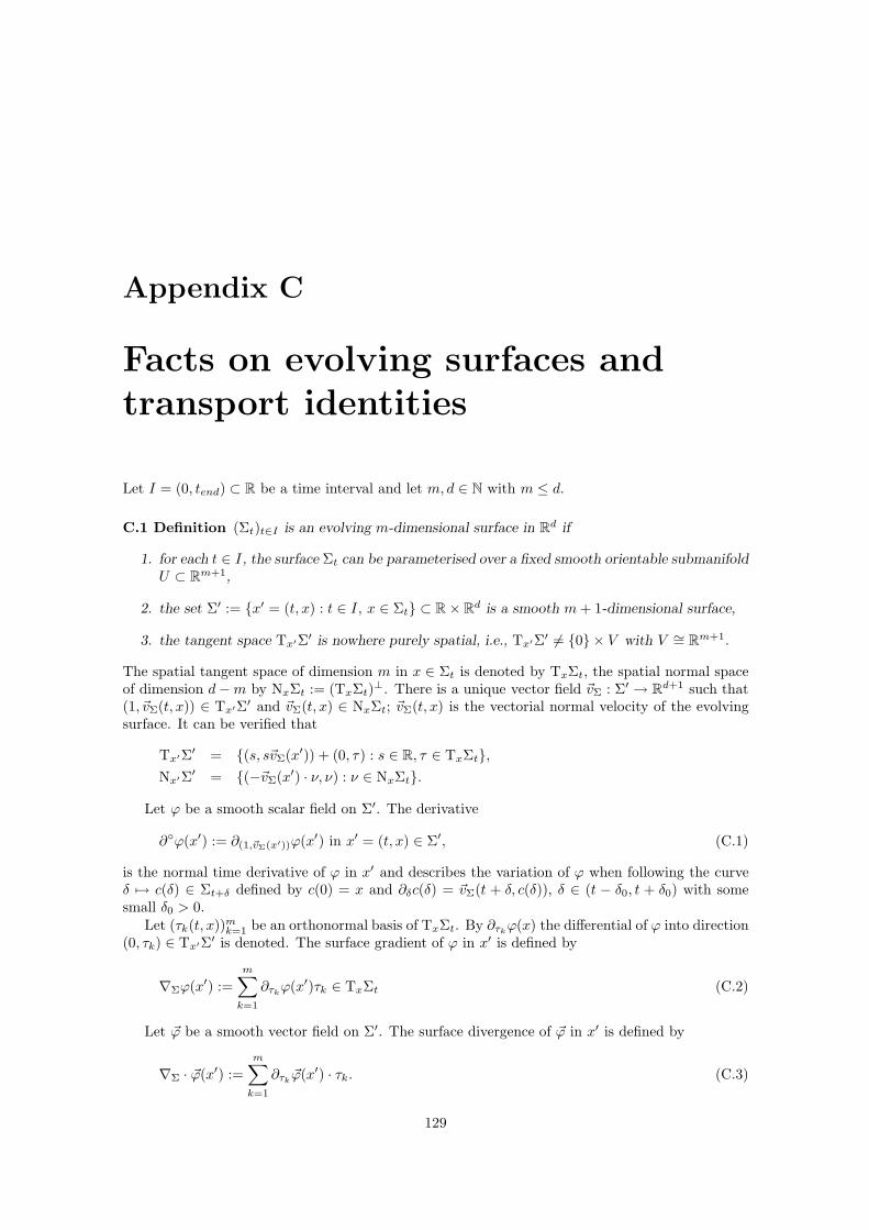
Appendix C

Facts on evolving surfaces andtransport identities

Let I = (0, tend) ⊂ R be a time interval and let m, d ∈ N with m ≤ d.

C.1 Definition (Σt)t∈I is an evolving m-dimensional surface in Rd if

1. for each t ∈ I, the surface Σt can be parameterised over a fixed smooth orientable submanifoldU ⊂ R

m+1,

2. the set Σ′ := x′ = (t, x) : t ∈ I, x ∈ Σt ⊂ R × Rd is a smooth m + 1-dimensional surface,

3. the tangent space Tx′Σ′ is nowhere purely spatial, i.e., Tx′Σ′ 6= 0 × V with V ∼= Rm+1.

The spatial tangent space of dimension m in x ∈ Σt is denoted by TxΣt, the spatial normal spaceof dimension d − m by NxΣt := (TxΣt)

⊥. There is a unique vector field ~vΣ : Σ′ → Rd+1 such that

(1, ~vΣ(t, x)) ∈ Tx′Σ′ and ~vΣ(t, x) ∈ NxΣt; ~vΣ(t, x) is the vectorial normal velocity of the evolvingsurface. It can be verified that

Tx′Σ′ = (s, s~vΣ(x′)) + (0, τ) : s ∈ R, τ ∈ TxΣt,Nx′Σ′ = (−~vΣ(x′) · ν, ν) : ν ∈ NxΣt.

Let ϕ be a smooth scalar field on Σ′. The derivative

∂ϕ(x′) := ∂(1,~vΣ(x′))ϕ(x′) in x′ = (t, x) ∈ Σ′, (C.1)

is the normal time derivative of ϕ in x′ and describes the variation of ϕ when following the curveδ 7→ c(δ) ∈ Σt+δ defined by c(0) = x and ∂δc(δ) = ~vΣ(t + δ, c(δ)), δ ∈ (t − δ0, t + δ0) with somesmall δ0 > 0.

Let (τk(t, x))mk=1 be an orthonormal basis of TxΣt. By ∂τk

ϕ(x) the differential of ϕ into direction(0, τk) ∈ Tx′Σ′ is denoted. The surface gradient of ϕ in x′ is defined by

∇Σϕ(x′) :=

m∑

k=1

∂τkϕ(x′)τk ∈ TxΣt (C.2)

Let ~ϕ be a smooth vector field on Σ′. The surface divergence of ~ϕ in x′ is defined by

∇Σ · ~ϕ(x′) :=

m∑

k=1

∂τk~ϕ(x′) · τk. (C.3)

129

APPENDIX C. FACTS ON EVOLVING SURFACES AND TRANSPORTIDENTITIES

If m = d − 1 the normal space NxΣt has dimension one, and Σ′ is orientable. Then there is asmooth vector field νΣ of unit normals, νΣ(x′) ∈ NxΣt, |νΣ(x′)|2 = 1. The (scalar) curvature andthe curvature vector then are defined by

κΣ := −∇Σ · νΣ, ~κΣ := κΣνΣ. (C.4)

Moreover, the (scalar) normal velocity then is defined by

vΣ = ~vΣ · νΣ, (C.5)

and the following relation, derived in [Gur00], Chapter 15b, holds:

∂νΣ = −∇ΣvΣ. (C.6)

C.2 Definition Γ′ := (Γt)t is an evolving m-dimensional subsurface of Σ′ if

1. the set Γt is a relatively open connected subset of Σt for each t ∈ I,

2. the boundary ∂Γ′ := (∂Γt)t consists of a finite number of evolving m−1-dimensional surfacessuch that, locally for each t ∈ I, ∂Γt is the graph of a Lipschitz continuous map.

A vectorial normal velocity ~v∂Γ can be assigned to the pieces of ∂Γ′ while Γ′ obviously has the samevectorial normal velocity as Σ′, namely ~vΣ.

In some point x ∈ ∂Γt the tangent cone on Γt is denoted by TxΓt. If x is in the interior ofone of the pieces the cone is a half-space of TxΣt. Besides then the boundary of TxΓt in TxΣt

coincides with the tangent space of the boundary ∂Γt, i.e., ∂TxΓt = Tx∂Γt. In such points x thereis a unique unit vector τΓ ∈ TxΣt ∩ Nx∂Γt with

τΓ · τ ≤ 0 for all τ ∈ TxΓt. (C.7)

This vector τΓ is said to be the external unit normal of Γt with respect to Σt. For example, inFigure 1.1 where d = 2 and m = 1, the external unit normal of Γαβ in the triple junction is ταβ . Aset corresponding to Σt can be obtained by smoothly extending Γαβ over the triple junction.

Let m = d − 1 and d ≤ 3. First, a divergence theorem is stated for a smooth surface withpiecewise smooth Lipschitz boundary like Γt as in Definition C.2:

C.3 Theorem ([Bet86], Corollary 4 ) In the above described situation there is the followingidentity:

∫

Γt

(∇Σ · ~ϕ + ~κΣ · ~ϕ) dHm(x) =

∫

∂Γt

~ϕ · τΓdHm−1. (C.8)

If ~ϕ is a tangent vector field then ~κΣ · ~ϕ = 0 so that one gets the usual divergence theorem onsurfaces. It should be remarked that the proof in [Bet86] is performed for smooth ∂Γt but there isa brief note on the above case of a piecewise smooth boundary at the end of Section II(2). Next, atransport identity is stated:

C.4 Theorem ([Bet86], Theorem 1) In the above described situation it holds for every t ∈ I that

d

dt

(∫

Γt

ϕdHm

) ∣∣∣∣t

=

∫

Γt

(∂ϕ − ϕ~vΣ · ~κΣ) dHm +

∫

∂Γt

(ϕ~v∂Γ · τΓ) dHm−1. (C.9)

C.5 Remark If ~vΣ = 0 and ~κΣ = 0 then Γt is flat, ∂ reduces to ∂t and ~v∂Γ is tangential.Altogether, the Reynold’s transport theorem is obtained.

130

Appendix D

Several functional analyticalresults

This chapter contains a list a important facts for chap. 4 including references.

D.1 Theorem (Picard-Lindelof, cf. [Wal96], Theorem II.§10.VI.) Let 0 ∈ (−δ, a) ⊂ R bean open interval and D ⊂ R

n an open domain. Let f ∈ C0((−δ, a)×D) be Lipschitz continuous withrespect to the second variable, i.e., there is a constant L > 0 such that |f(t, y)− f(t, y)| ≤ L|y − y|or all y, y ∈ D, t ∈ (−δ, a).

Let y0 ∈ D. Then the initial value problem

y′(t) = f(t, y(t)), y(0) = y0

has a unique solution which can be extended to both sides of t = 0 until reaching the boundary.

D.2 Theorem (Lebesgue, cf. [Alt99], Theorem 1.21) Consider a set D ⊂ Rd and p ∈ [1,∞).

For k ∈ N, let gk → g in L1(D; R) as k → ∞ and let fk, f : D → Y be measurable functions mappinginto some Banach space Y such that

(i) fk → f almost everywhere as k → ∞,

(ii) |fk|p ≤ gk almost everywhere for all k.

Then fk, f ∈ Lp(D; Y ) and

fk → f in Lp(D; Y ) as k → ∞.

D.3 Theorem (Rellich, cf. [Alt99], Theorem A6.4) Let D ⊂ Rd be an open, bounded do-

main with Lipschitz boundary, 1 ≤ p < ∞ and m ≥ 1. For k ∈ N, let fk, f ∈ Wm,p(D). Then, ask → ∞,

fk f in Wm,p(D) ⇒ fk → f in Wm−1,p(D).

D.4 Theorem (Sobolev, cf. [Alt99], Theorem 8.9) Let D ⊂ Rd be an open, bounded domain

with Lipschitz boundary, 1 ≤ p1, p2 < ∞ and m1, m2 ≥ 0.

1. If m1 − dp1

≥ m2 − dp2

and m1 ≥ m2 then there is the continuous embedding

Hm1,p1(D) → Hm2,p2(D).

2. If m1 − dp1

> m2 − dp2

and m1 > m2 then the above embedding is compact.

131

APPENDIX D. SEVERAL FUNCTIONAL ANALYTICAL RESULTS

D.5 Theorem (Cf. [Alt99], Theorem 8.5) Let D ⊂ Rd be an open, bounded domain with

Lipschitz boundary. Then the embedding

Ck,1(D) → W k+1,∞(D)

exists and is an isomorphism (in the sense that to each f ∈ W k+1,∞(D) there is a function f ∈Ck,1(D) with f = f almost everywhere). In particular, it holds that

W k+1,∞(R) → Ck,1(R).

D.6 Theorem (Trace theorem, cf. [Alt99], Theorem A6.6 and A6.13) Let the set Ω ⊂ Rd

be an open, bounded domain with Lipschitz boundary and 1 ≤ p ≤ ∞. There is a unique linearcontinuous map

S : W 1,p(Ω) → Lp(∂Ω)

such that

S(f) = f∣∣∂Ω

for all f ∈ W 1,p(Ω) ∩ C0(Ω).

Let now p < ∞. For k ∈ N, let fk, f ∈ W 1,p(D). Then, as k → ∞,

fk f in W 1,p(D) ⇒ fk → f in Lp(∂D).

D.7 Lemma (Gronwall lemma, cf. [Wal96], V.§29.X.) Let f ∈ C0([0, β]; R) satisfying

f(t) ≤ α +

∫ t

0

h(r)f(r)dr

where α ∈ R and h ∈ L1([0, β]) is nonnegative (almost everywhere). Then

f(t) ≤ αeH(t) where H(t) =

∫ t

0

h(r)dr.

D.8 Theorem (Cf. [Zei90], Ex. 23.13) Let I = (0, T ) ⊂ R be an open interval and let X, Y, Zbe real Banach spaces. Consider the set

W :=u ∈ Lp(I; X), u′ ∈ Lq(I; Z)

.

1. The embedding W → C0(I ; Z) exists and is continuous provided

(i) the embedding X → Z is continuous,

(ii) it holds that 1 ≤ p, q ≤ ∞.

2. The embedding W → Lp(I; Y ) exists, is continuous, and is compact provided

(i) there are continuous embeddings X → Y → Z,

(ii) the embedding X → Y is compact,

(iii) the spaces X and Z are reflexive,

(iv) it holds that 1 < p, q < ∞.

D.9 Theorem (Convolution estimate, cf. [Alt99], Theorem 2.12) Let ζ ∈ L1(Rd) and f ∈Lp(Rd; Y ) with some Banach space Y , and let p ∈ [1,∞]. Then by

(ζ ∗ f)(x) :=

∫

Rd

ζ(x − y)f(y)dy =

∫

Rd

ζ(y)f(x − y)dy (D.1)

132

a function ζ ∗ f ∈ Lp(Rd; Y ) is defined satisfying

‖ζ ∗ f‖Lp(Rd;Y ) ≤ ‖ζ‖L1(Rd)‖f‖Lp(Rd;Y ). (D.2)

If f has weak derivatives then the weak derivatives of ζ ∗ f are the convolutions of the weakderivatives of f with ζ, i.e.

∂α(ζ ∗ f) = ζ ∗ ∂αf (D.3)

where α = (α1, . . . , αd) is some multi-index indicating the derivatives with respect to the variablescorresponding to (x1, . . . , xd).

D.10 Definition (Dirac sequences) A sequence (ζk)k∈N in L1(Rd) is a Dirac sequence if

ζk ≥ 0,

∫

Rd

ζk = 1,

∫

Rd\Bρ(0)

ζk → 0 as k → ∞ for all ρ > 0. (D.4)

If ζ ∈ L1(Rd) fulfils ζ ≥ 0 and∫

Rd ζ = 1 then the sequence (ζε)ε>0 defined by

ζε(x) := ε−dζ(x

ε

)(D.5)

is the Dirac sequence associated to ζ.

D.11 Theorem (Cf. [Alt99], Theorem 2.14) Let (ζk)k be a Dirac sequence, Y be a Banachspace, p ∈ [1,∞), and let f ∈ Lp(Rd; Y ). Then

ζk ∗ f → f in Lp(Rd; Y ) as k → ∞. (D.6)

D.12 Theorem (Vitali, cf. [Alt99], Theorem 1.19) Consider a bounded domain D ⊂ Rd and

p ∈ [1,∞). For k ∈ N, let fk, f : D → Y be measurable functions mapping into some Banach spaceY such that fk → f as k → ∞ almost everywhere, and assume fk ∈ Lp(D; Y ).

Then fk → f in Lp(D; Y ) if and only if

supk

∫

E

|fk|p dx → 0 as Ld(E) → 0.

D.13 Lemma (Fatou, cf. [Alt99], Lemma A1.19) Consider a domain D ⊂ Rd and let fkk

be a set of non-negative integrable functions on D. Then∫

D

lim infk→∞

fk(x) dx ≤ lim infk→∞

∫

D

fk(x) dx.

D.14 Lemma (Poincare inequality, cf. [Alt99], Theorem 6.15) Let the set D ⊂ Rd be an

open bounded domain with Lipschitz boundary ∂D. Let J ⊂ W 1,p(D; Rk) be a nonempty, convex,and closed subset with some p ∈ (1,∞). The following points are equivalent:

1. There is some f0 ∈ J and some C0 > 0 such that for all v ∈ Rk with f0 + v ∈ J it follows

that |v| ≤ C0.

2. A constant C > 0 exists so that for all f ∈ J

‖f‖Lp(D;Rk) ≤ C(‖∇f‖Lp(D;(Rk)d) + 1

). (D.7)

D.15 Theorem (Riesz, cf. [Alt99], Theorem 2.15) Let p ∈ [1,∞). A set A ⊂ Lp(Rd) isprecompact if and only if there is a constant C > 0 such that

(i) supf∈A ‖f‖Lp ≤ C,

(ii) supf∈A ‖f(· − h) − f‖Lp → 0 as |h| → 0,

(iii) supf∈A ‖f‖LP (Rd\BR(0)) → 0 as R → ∞.

133

134

Bibliography

[AB98] G. Alberti and G. Bellettini. A non-local anisotropic model for phase transitions:asymptotic behaviour of rescaled energies. Europ. J. Appl. Math. 9, pp. 261-284, 1998.

[ABC94] N. D. Alikakos, P. Bates, and X. Chen. Convergence of the Cahn-Hilliard equation tothe Hele-Shaw model. Arch. Rat. Mech. Anal. 128, pp. 165-205, 1994.

[AL83] H. W. Alt and S. Luckhaus. Quasilinear elliptic-parabolic differential equations. Math.Z. 183, pp. 311-341, 1983.

[Alm99] R. F. Almgren. Second-order phase field asymptotics for unequal conductivities. SIAMJ. Appl. Math. 59, pp. 2086-2107, 1999.

[Alt99] H. W. Alt. Lineare Funktionalanalysis. 3. ed., Springer, ISBN 3-540-65421-6, 1999.

[And02] C. Andersson. Third order asymptotics of a phase-field model. TRITA-NA-0217, Dep.of Num. Anal. and Comp. Sc., Royal Inst. of Technology, Stockholm, 2002.

[AP92] H. W. Alt and I. Pawlow. A mathematical model of dynamics of non-isothermal phaseseparation. Phys. D 59, pp. 389-416, 1992.

[AP93] H. W. Alt and I. Pawlow. Solutions for a model of nonisothermal phase separation.Free boundary problems involving solids (Montreal, PQ, 1990), pp. 214-219, PitmanRes. Notes Math. Ser., 281, Longman Sci. Tech., Harlow, 1993.

[BBR05] G. Bellettini, A. Braides, and G. Riey. Variational approximation of anisotropic func-tionals on partitions. Annali di matematica 184, pp. 75-93, 2005.

[BE93] J.F. Blowey and C.M. Elliott. Curvature dependent phase boundary motion andparabolic double obstacle problems. Degenerate diffusions (Minneapolis, MN, 1991).IMA Vol. Math. Appl. 47, Springer, pp. 19-60, 1993.

[Bet86] D. E. Betounes. Kinematics of submanifolds and the mean curvature normal. Arch.Rat. Mech. Anal. 96, pp. 1-27, 1986.

[BGS98] L. Bronsard, H. Garcke, and B. Stoth. A multi-phase Mullins–Sekerka system: Matchedasymptotic expansions and an implicit time discretization for the geometric evolutionproblem. Proc. Roy. Soc. Edinburgh Sect. A 128, pp. 481-506, 1998.

[Cag89] G. Caginalp. Stefan and Hele Shaw type models as asymptotic limits of the phase fieldequations. Phys. Rev. A 39, pp. 5887-5896, 1989.

[CC98] G. Caginalp and X. Chen. Convergence of the phase field model to its sharp interfacelimits. European J. Appl. Math. 9, pp. 417-445, 1998.

[CF88] G. Caginalp and P. C. Fife. Dynamics of layered interfaces arising from phase bound-aries. SIAM J. Appl. Math. 48, pp. 506-518, 1988.

135

[CH58] J. W. Cahn and J. E. Hilliard. Free Energy of a Nonuniform System. I. Interfacial FreeEnergy. J. Chem. Phys. 28, pp. 258-267, 1958.

[CH74] J. W. Cahn and D. W. Hoffmann. A vector thermodynamics for anisotropic surfacesII. Curved and faceted surfaces. Acta Metall. Mater. 22, pp. 1205-1214, 1974.

[Che02] L. Q. Chen. Phase-field models for microstructural evolution. Ann. Rev. Mater. Res.32, pp. 113-140, 2002.

[Dar49] L. Darken. Diffusion of carbon in austenite with a discontinuity in composition. TransAIME 180, pp. 430-438, 1949.

[Dav01] S. H. Davis. Theory of solidification. Cambridge University Press, ISBN 0-521-65080-1,2001.

[Eck04] C. Eck. A Two-Scale Phase Field Model for Liquid-Solid Phase Transitions of Bi-nary Mixtures with Dendritic Microstructure. Habilitationsschrift, Universitat Erlan-gen, 2004.

[ET99] I. Ekeland and R. Temam. Convex analysis and variational problems. Unabridged, corr.republ. of the work 1. publ. in English Amsterdam and New York, 1976, Classics inapplied mathematics 28, Philadelphia Soc. for Industrial and A, ISBN 0-89871-450-8,1999.

[FP95] P.C. Fife and O. Penrose. Interfacial dynamics for thermodynamically consistent phase-field models with nonconserved order parameter. EJDE 1995, No. 16, pp. 1-49, 1995.

[Gar02] H. Garcke. Einfuhrung in die mathematische Modellierung. Lecture notes, NWF I -Mathematik, University of Regensburg, summer term 2002.

[GHS05] H. Garcke, R. Haas, and B. Stinner. On Ginzburg-Landau type free energies for multi-phase systems. In preparation, 2005.

[Giu77] E. Giusti. Minimal surfaces and functions of bounded variation. Notes on Pure Math-ematics 10, Australian National Univ., Canberra, ISBN = 0-7081-1294-3, 1977.

[GN00] H. Garcke and B. Nestler. A mathematical model for grain growth in thin metallic films.Math. Models and Methods in Applied Sciences, Vol. 10, pp. 895-921, 2000.

[GNC00] H. Garcke and A. Novick-Cohen. A singular limit for a system of degenerate Cahn-Hilliard equations. Adv. Differential Equations 5, pp. 401-434, 2000.

[GNS98] H. Garcke, B. Nestler, and B. Stoth. On anisotropic order parameter models for multi-phase systems and their sharp interface limits. Phys. D 115, pp. 87-108, 1998.

[GNS99a] H. Garcke, B. Nestler, and B. Stoth. Anisotropy in multi-phase systems: A phase fieldapproach. Interfaces Free Bound. 1, pp. 175-198, 1999.

[GNS99b] H. Garcke, B. Nestler, and B. Stoth. A multiphase field concept: Numerical simulationsof moving phase boundaries and multiple junctions. SIAM J. Appl. Math. 60, pp. 295-315, 1999.

[Gur93] M. E. Gurtin. Thermomechanics of evolving phase boundaries in the plane. ClarendonPress, Oxford, ISBN 0-19-853694-1, 1993.

[Gur00] M. E. Gurtin. Configurational forces as basic concepts of continuum physics. Appl.Math. Sc. 137, Springer, ISBN 0-387-98667-7, 2000.

[Haa94] P. Haasen. Physikalische Metallkunde. 3. ed., Springer, ISBN 3-540-57210-4, 1994.

136

[HLS96] W. Horn, P. Laurencot, and J. Sprekels. Global solutions to a Penrose-Fife phase-field model under flux boundary conditions for the inverse temperature. Math. MethodsAppl. Sci. 19. pp. 1053–1072, 1996.

[JH66] K. A. Jackson and J. D. Hunt. Lamellar and rod eutectic growth. Trans. Metall. Soc.AIME 236, p. 1129-1142, 1966.

[Kar01] A. Karma. Phase-field formulation for quantitative modeling of alloy solidification.Phys. Rev. Lett. 87, pp. 115701-1-4, 2001.

[KKS99] S.-G. Kim, W.-T. Kim, and T. Suzuki. Phase-field model for binary alloys. Phys. Rev.E, Vol. 60, No. 6, pp. 7186-7197, 1999.

[Kle02] O. Klein. Existence and approximation of solutions to an anisotropic phase field systemfor the kinetics of phase transitions. Interfaces Free Bound. 4, pp. 47–70, 2002.

[KR98] A. Karma and J.-W. Rappel. Quantitative phase-field modeling of dendritic growth intwo and three dimensions. Phys. Rev. E 57, pp. 4323-4349, 1998.

[KRS05] P. Krejci, E. Rocca, and J. Sprekels. Nonlocal temperature-dependent phase-field modelsfor non-isothermal phase transitions. WIAS Preprint No. 1006, 2005.

[KY87] J. S. Kirkaldy and D. J. Young. Diffusion in the condensed state. The Institute ofMetals, London, ISBN 0-904357-87-2, 1987.

[Lan86] J.S. Langer. Models of pattern formation in first–order phase transitions. Directions inCondensed Matter Physics, World Scientific, Singapore, pp. 165-186, 1986.

[LG50] L. D. Landau and V. I. Ginzburg. K teorii sverkhrovodimosti. Zh. Eksp. Teor. Fiz20, pp. 1064-1082 (english translation: On the theory of superconductivity, CollectedPapers of L.D. Landau, D. ter Haar, ed., Pergamon, Oxford, UK, pp. 626-633 (1965)),1950.

[LP88] P.-A. Lagerstrom and A. Paco. Matched asymptotic expansions : ideas and techniques.Appl. Math. Sc. 76, Springer, ISBN 0-387-96811-3, 1988.

[Luc91] S. Luckhaus. The Stefan problem with the Gibbs Thompson law. Report univ. Pisa 591,1991.

[LV83] S. Luckhaus and A. Visintin. Phase transition in multicomponent systems. Man. Math.43, pp. 261-288, 1983.

[Mod87] L. Modica. The gradient theory of phase transitions and the minimal interface criterion.Arch. Rat. Mech. Anal. 98, pp. 123-142, 1987.

[MS95] P. De Mottoni and M. Schatzman. Geometrical evolution of developed interfaces. Trans.Amer. Math. Soc. Vol. 347, pp. 1533-1589, 1995.

[Mul01] I. Muller. Grundzuge der Thermodynamik. 3. ed., Springer, ISBN = 3-540-42210-2,2001.

[MWA00] G.B. McFadden, A.A. Wheeler, and D.M. Anderson. Thin interface asymptotics foran energy/entropy approach to phase-field models with unequal conductivities. Phys. D144, pp. 154-168, 2000.

[NGS05] B. Nestler, H. Garcke, and B. Stinner. Multicomponent alloy solidification: Phase-fieldmodelling and simulations. Phys. Rev. E 71, pp. 041609-1-6, 2005.

137

[OKS01] M. Ode, S.-G. Kim, and T. Suzuki. Recent advances in the phase-field model forsolidification. ISIJ International 41, pp. 1076-1082, 2001.

[Ons31] L. Onsager. Reciprocal relations in irreversible processes I. Phys. Rev. 37, pp. 405-426,1931.

[PF90] O. Penrose and P. C. Fife. Thermodynamically consistent models of phase field type forthe kinetics of phase transition. Phys. D 43, pp. 44-62, 1990.

[RBKD04] J. C. Ramirez, C. Beckermann, A. Karma, and H.-J. Diepers. Phase-field modeling ofbinary alloy solidification with coupled heat and solute diffusion. Phys. Rev. E 69, pp.51607-1-16, 2004.

[RK48] O. Redlich and A. T. Kister. Algebraic Representation of Thermodynamic Propertiesand the Classification of Solutions. Indust. Eng. Chem. 40, pp. 345-348, 1948.

[Sch98] A. Schmidt. Approximation of crystalline dendrite growth in two space dimensions.Acta Math. Univ. Com. 86, pp. 57-68, 1998.

[Smo94] J. Smoller. Shock Waves and Reaction-Diffusion Equations. 2. ed., Grundlehren derMath. Wissenschaften 258, Springer, ISBN 3-540-94259-9, 1994.

[SPN+96] I. Steinbach, F. Pezolla, B. Nestler, M. Seeßelberg, R. Prieler, G. J. Schmitz, andJ. L. L. Rezende. A phase field concept for multi phase systems. Phys. D 94, pp.35-147, 1996.

[Ste91] P. Sternberg. Vector-valued local minimizers of nonconvex variational problems. RockyMountain J. Math. 21, pp. 799-807, 1991.

[Sto96] B. Stoth. A sharp interface limit of the phase field equations, one-dimensional andaxisymmetric. Europ. J. Appl. Math. 7, pp. 603-633, 1996.

[SZ03] J. Sprekels and S. Zheng. Global existence and asymptotic behaviour for a nonlocalphase-field model for non-isothermal phase transitions. J. Math. Anal. Appl. 279, pp.97–110, 2003.

[TAV03] K. Thornton, J. Agren, and P. W. Voorhees. Modelling the evolution of phase boundariesin solids at the meso- and nano-scales. Acta Mat. 51, pp. 5675-5710, 2003.

[TC94] J. E. Taylor and J. W. Cahn. Linking anisotropic sharp and diffuse motion laws viagradient flows. J. Stat. Phys. 77, pp. 183-197, 1994.

[vdW83] J. D. van der Waals. The thermodynamic theory of capillarity under the hypothesis of acontinuous variation of density. Konink. Nederl. Akad. Wetensch. Afd. Natuurk. EersteReeks, 1 (english translation with commentary: J. S. Rowlinson, J. Statist. Phys. 20 ,pp. 197-244 (1979)), 1983.

[Wal96] W. Walter. Gewohnliche Differentialgleichungen. 6. ed., Springer, ISBN 3-540-59038-2,1996.

[WM97] A. A. Wheeler and G. B. McFadden. On the notion of a ξ-vector and a stress tensorfor a general class of anisotropic diffuse interface models. Proc. Roy. Soc. London Ser.A 453, pp. 1611-1630, 1997.

[WMB92] A.A. Wheeler, G. B. McFadden, and W. J. Boettinger. Phase-fiel model for isothermalphase transitions in binary alloys. Phys. Rev. A 45, pp. 7424-7439, 1992.

138

[WSW+93] S.-L. Wang, R. F. Sekerka, A. A. Wheeler, B. T. Murray, S. R. Coriell, R. J. Braun, andG. B. McFadden. Thermodynamically-consistent phase-field models for solidification.Physica D 69, pp. 189-200, 1993.

[Zei90] E. Zeidler. Nonlinear functional analysis and its applications II/A, linear monotoneoperators. Springer, ISBN 0-387-96802-4, 1990.

epub.uni-regensburg.de · Contents 1 Alloy Solidiﬁcation 11 1.1 Irreversible thermodynamics . . . . . . . . . . . . . . . . . . . . . . . . . . . . . . . . 11 1.1.1 Thermodynamics

Documents