Eocene-Oligocene Transition Deep Sea Temperature and Saturation State Changes from Benthic Foraminiferal Trace Metal Analysis

Eocene-Oligocene Transition Deep Sea Temperature

and Saturation State Changes from Benthic

Foraminiferal Trace Metal Analysis

John S. Crowe

Master of Earth Science

Marine Geoscience (International)

April 2015

School of Earth and Ocean Sciences, Cardiff University, Main Building, Park

Place, Cardiff, UK, CF10 3AT

We live on a planet that has a more or less infinite capacity to surprise. What

reasoning person could possibly want it any other way?

-Bill Bryson

3

DECLARATION

STATEMENT

This work has not previously been accepted in substance for any degree and is not being

concurrently submitted in candidature for any degree.

Signed: ________________________________ (candidate)

Date: __________________________________

STATEMENT

This dissertation is being submitted in partial fulfilment of the requirements for the degree of

Master of Earth Sciences.


Date: __________________________________

STATEMENT

This dissertation is the result of my own independent work, except where otherwise stated.


Date: __________________________________

4

Abstract

The climate transition that occurs at the Eocene-Oligocene boundary (~33.7 Ma) is marked by the first

significant Antarctic glaciation of the Cenozoic. Across the Eocene-Oligocene transition, two upward

shifts in deep sea benthic foraminiferal isotope (δ18O) values occur, Step 1 and Step 2. These shifts in

δ18O reflect a combination of bottom water temperature and δ18O of seawater. Published

paleotemperature records, calculated from foraminiferal Mg/Ca, do not show a cooling across the

Eocene-Oligocene transition, potentially indicating a saturation state effect on benthic foraminiferal

Mg/Ca during this period.

This thesis attempts to ascertain the saturation state history of Ocean Drilling Program Site 757

through the use of benthic foraminiferal trace metal climate proxies. Inductively coupled plasma mass

spectrometry was used to analyse the trace metal geochemistry of two benthic foraminifera species,

Bulimina jarvisi (n=56) and Cibicidoides havanensis (n=62). An infaunal and epifaunal benthic

foraminifera species were chosen, enabling an assessment to be made of how saturation state change

effects the different microhabitats inhabited by foraminifera. Quantification of saturation state change

enabled benthic foraminiferal Mg/Ca values to be corrected for any saturation state effect, allowing

accurate paleotemperature change to be determined. By calculating accurate changes in past bottom

water temperature, it was possible to quantify change in δ18O of seawater and thus ice growth and sea

level change.

Here we present data that shows a clear rise in infaunal (0.12 mmol/mol) and epifaunal (0.06

mmol/mol) benthic foraminiferal Mg/Ca across the Eocene-Oligocene transition. Further, a clear

increase in saturation state (18.17 µmol kg-1) was shown for the same period. By correcting Mg/Ca

paleotemperatures for saturation state change, it was found that bottom water temperature cooled

across the Eocene-Oligocene transition (~1.5 ⁰C). The timings of the cooling and warming events

across the Eocene-Oligocene transition, with regard to the two δ18O isotope shifts, do not easily

correlate with published records. To some degree, both δ18O shifts appear to be associated with

warming and ice growth. Across the Eocene-Oligocene transition, sea level has been shown to fall

(~50m), however sea level appears to rise as well as fall during this period.

This study concluded that non saturation state corrected temperatures calculated from infaunal

foraminifera are not accurate or reliable indicators of changes in bottom water temperature. Despite

accounting for saturation state change, warming periods across the Eocene-Oligocene climate

transition were discovered here. These warming periods are associated with the two shifts in δ18O

values, Step 1 and Step 2. Significant periods of ice growth were associated also with the shifts.

5

Table of Contents

1. INTRODUCTION ................................................................................................................ 8

1.1. Foraminiferal Stable Isotope Analysis ......................................................................... 9

1.1.1. Oxygen ................................................................................................................. 9

1.1.2. Carbon ................................................................................................................ 10

1.2. Carbonate System ...................................................................................................... 11

1.3. Foraminiferal Test Mass as a Proxy for Carbonate Saturation State ......................... 13

1.4. Benthic Foraminiferal Abundance as a Proxy for Productivity ................................. 14

1.5. Trace Metal/Calcium Proxies Using Benthic Foraminifera....................................... 15

1.5.1. Mg/Ca ................................................................................................................. 15

1.5.2. Li/Ca ................................................................................................................... 19

1.5.3. B/Ca .................................................................................................................... 21

1.5.4. Sr/Ca ................................................................................................................... 23

1.5.5. U/Ca .................................................................................................................... 24

1.6. Eocene-Oligocene Transition .................................................................................... 27

1.6.1. Oxygen Stable Isotope Records .......................................................................... 27

1.6.2. Trace Metal Records ........................................................................................... 28

1.6.3. Proposed Mechanisms for EOT Initiation .......................................................... 29

1.7. Regional and Geological Setting ............................................................................... 31

1.8. Benthic Foraminiferal Biostratigraphy of ODP Hole 757B ...................................... 32

1.9. Pilot Ostracod Study .................................................................................................. 33

1.10. Motivation .............................................................................................................. 37

1.10.1. Hypothesis ...................................................................................................... 37

2. MATERIALS AND METHODS ....................................................................................... 39

2.1. Sampling .................................................................................................................... 40

6

2.1.1. Species Selection ................................................................................................ 40

2.2. Microscopy ................................................................................................................ 40

2.3. Weighing .................................................................................................................... 41

2.4. Sample Preparation and Chemical Cleaning.............................................................. 41

2.4.1. Crushing and Pre-Cleaning ................................................................................. 41

2.4.2. Cleaning Procedure............................................................................................. 41

2.5. Sample Dissolution and Calcium Concentration Analysis ........................................ 44

2.6. Trace Metal Analysis ................................................................................................. 44

2.7. Age Model ................................................................................................................. 46

2.8. Calculation of Temperature, Saturation State and Ice Volume ................................. 47

3. RESULTS ........................................................................................................................... 50

3.1. Microscopy ................................................................................................................ 51

3.2. Foraminiferal Average Test Masses .......................................................................... 52

3.3. Species Abundances .................................................................................................. 54

3.4. Foraminiferal Mg/Ca ................................................................................................. 56

3.5. Foraminiferal Li/Ca ................................................................................................... 58

3.6. Foraminiferal B/Ca .................................................................................................... 60

3.7. Foraminiferal Sr/Ca ................................................................................................... 62

3.8. Foraminiferal U/Ca .................................................................................................... 64

4. DISCUSSION ..................................................................................................................... 66

4.1. Bottom Water Temperature and Saturation State History at ODP Site 757 .............. 67

4.1.1. Bottom Water Temperature Calculated Using Mg/Ca of B. jarvisi ................... 67

4.1.2. Saturation State Change Calculated Using B/Ca of C. havanensis .................... 70

4.1.3. Support for Saturation State Change from Foraminiferal Test Mass ................. 72

4.1.4. Inter-Site Comparisons of Saturation State Change ........................................... 72

4.1.5. Corrected Bottom Water Temperature Change Using C. Havanensis ............... 74

7

4.1.6. Inter-Site Comparisons of Bottom Water Temperature Change ........................ 76

4.1.7. Changes in Ice Volume across the EOT ............................................................. 78

4.1.8. Inter-Site Comparisons of δ18Osw ....................................................................... 82

4.2. Indications from the Foraminiferal Li/Ca, Sr/Ca and U/Ca Records......................... 83

4.2.1. Li/Ca ................................................................................................................... 83

4.2.2. Sr/Ca ................................................................................................................... 85

4.2.3. U/Ca .................................................................................................................... 86

4.3. Surface Productivity Changes across the EOT .......................................................... 88

5. SUMMARY ....................................................................................................................... 90

5.1. Conclusions ................................................................................................................ 91

5.2. Further Work and Future Direction ........................................................................... 93

6. REFERENCES ................................................................................................................... 94

7. ACKNOWLEDGMENTS ................................................................................................ 102

8. APENDICES .................................................................................................................... 103

8.1. Appendix 1 ............................................................................................................... 103

8.2. Appendix 2 ............................................................................................................... 105

8.3. Appendix 3 ............................................................................................................... 114

1. INTRODUCTION

8

1. INTRODUCTION

Foraminiferal stable isotope analysis

Carbonate system

Foraminiferal test mass

Foraminiferal abundance

Trace metal/calcium proxies using benthic foraminifera

Eocene-Oligocene transition

Regional and geological setting

Biostratigraphy

Pilot ostracod study

Motivation

1. INTRODUCTION

9

The creation of an accurate record of past climate is essential to modern day climate science.

Records of past climate are used to test models which predict future change. Direct records of

past climate run from the mid-15th century to present. No indication of climate change outside

the last millennium is available from direct records. The climatic conditions which prevailed

during the Eocene-Oligocene transition (EOT) are studied in this work. The Eocene-

Oligocene transition coincided with the first glaciation of Antarctica during the Cenozoic. The

climatic conditions are ascertained by the use of foraminiferal geochemical proxies. This

introduction provides information on the proxies used, the regional setting of the sample sites

and the aims of the project.

1.1. Foraminiferal Stable Isotope Analysis

1.1.1. Oxygen

Oxygen stable isotope analysis is the most established geochemical proxy for recording past

climate conditions from foraminifera. Foraminiferal oxygen isotopes (δ18O) record both

temperature and sea water isotopic composition (δ18OSW). Ice growth increases δ18OSW

because 16O is concentrated in ice sheets by the hydrological cycle (Pearson, 2012). Melting

ice returns O16 dominated meltwater to the oceans, changing the ratio of the 16O to 18O. A

change in δ18O values can thus be temperature or ice growth related, providing an excellent

method for calculating past temperatures and ice volumes. A caveat when using stable oxygen

isotope ratios is that, in order to calculate either temperature or ice volume, the other variable

must be known. This variable can be calculated using other geochemical proxies, however

these are less accurate than using stable isotopes alone. During periods where no ice volume

change occurred, the 18O of a foraminifera may be used independently of seawater 18O to

quantify temperature. The 18O of a sample is calculated by comparing the ratio of both

oxygen isotopes to a standard of known isotopic composition (Equation 1.1).

EQN. (1.1)

18O sample (‰) = [(

𝑂18

𝑂16) 𝑠𝑎𝑚𝑝𝑙𝑒 − (𝑂18

𝑂16) 𝑠𝑡𝑎𝑛𝑑𝑎𝑟𝑑

(𝑂18

𝑂16) 𝑠𝑡𝑎𝑛𝑑𝑎𝑟𝑑]

The relationship between foraminiferal 18O, temperature and the 18O of seawater was

shown by Epstein et al. (1953) to follow equation 1.2:

1. INTRODUCTION

10

EQN. (1.2)

𝑇(0𝐶) = 𝐴 + 𝐵(δ18𝑂𝑠𝑎𝑚𝑝𝑙𝑒 − δ18𝑂𝑆𝑒𝑎𝑤𝑎𝑡𝑒𝑟) + 𝐶(δ18𝑂𝑠𝑎𝑚𝑝𝑙𝑒 − δ18𝑂𝑆𝑒𝑎𝑤𝑎𝑡𝑒𝑟)2

Where A, B and C represent experimentally derived coefficients.

In practice these relationships equate to ~0.21-0.23 ‰ decrease in the δ18O of calcite for

every 1 ⁰C increase in temperature.

1.1.2. Carbon

Two commonly used carbon isotopes (C12 and C13) are helpful in unravelling past climatic

trends. Equation 1.3 shows how 13C of a foraminifera is calculated from the isotopic ratio of

C13 to C12 and a standard of known isotopic composition (Rohling and Cooke, 2003). This

proxy monitors past changes in carbon reservoirs. Three major signals are recorded by 13C.

Firstly, isotopically light carbon is added to bottom waters when organic matter is oxidised.

Secondly, younger waters are isotopically heavier than older waters. If differently aged waters

are mixed a new 13C value is created. Finally, high productivity concentrates C12 within

organic matter. This process in turn concentrates C13 within the total dissolved carbonate that

reaches the bottom waters. Therefore, at any one time, benthic foraminiferal 13C may record

the 13C of the total dissolved carbonate in the a water mass, ocean circulation patterns and

productivity change (Ravelo and Hillaire-Marcel, 2007).

EQN. (1.3)

13C sample (‰) = [(

𝐶13

𝐶12) 𝑠𝑎𝑚𝑝𝑙𝑒 − (𝐶13

𝐶12) 𝑠𝑡𝑎𝑛𝑑𝑎𝑟𝑑

(𝐶13

𝐶12) 𝑠𝑡𝑎𝑛𝑑𝑎𝑟𝑑]

1. INTRODUCTION

11

1.2. Carbonate System

An understanding of the carbonate system is required in order to decipher the mechanisms

controlling the Eocene-Oligocene Transition climate. The carbonate system plays an

important role in calcareous microfossil shell chemistry, a key tool used to identify past

climatic events.

Calcium carbonate (CaCO3) solubility increases in waters with low pH or low temperatures or

increased pressure. The point at which no more CaCO3 can be dissolved into solution is

termed the calcium carbonate saturation point. A water mass containing a higher

concentration of solute than the saturation point is oversaturated while a water mass with a

lower concentration is termed undersaturated. Therefore, for dissolution to occur, a water

mass must be undersaturated with respect to calcium carbonate and environmental solubility

conditions must be favourable.

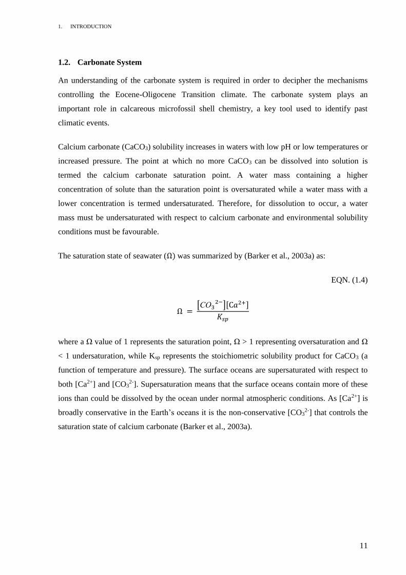
The saturation state of seawater (Ω) was summarized by (Barker et al., 2003a) as:

EQN. (1.4)

Ω = [CO3

2−][C𝑎2+]

𝐾𝑠𝑝

where a Ω value of 1 represents the saturation point, Ω > 1 representing oversaturation and Ω

< 1 undersaturation, while Ksp represents the stoichiometric solubility product for CaCO3 (a

function of temperature and pressure). The surface oceans are supersaturated with respect to

both [Ca2+] and [CO32-]. Supersaturation means that the surface oceans contain more of these

ions than could be dissolved by the ocean under normal atmospheric conditions. As [Ca2+] is

broadly conservative in the Earth’s oceans it is the non-conservative [CO32-] that controls the

saturation state of calcium carbonate (Barker et al., 2003a).

1. INTRODUCTION

12

Changing partial pressures of atmospheric CO2 (PCO2atm) affect ocean carbonate chemistry

through the following reactions:

EQN. (1.5)

𝐶𝑂2 𝑎𝑡𝑚 + 𝐻2𝑂 ↔ 𝐻2𝐶𝑂3 ↔ 𝐻+ + 𝐻𝐶𝑂3

− ↔ 2𝐻+ + 𝐶𝑂3 2−

When CO2 dissolves in the oceans, carbonic acid (𝐻2𝐶𝑂3) is formed. Subsequently, the

carbonic acid disassociates into bicarbonate (𝐻𝐶𝑂3 −) and hydrogen (H+) ions. Le Chatelier's

principle states, any change to one side of a reaction will promote an opposing reaction, which

will shift equilibrium thus minimizing the effect of the change. With this in mind, an increase

in PCO2atm will result in the reactions presented in equation 1.5 shifting toward the right. The

[𝐶𝑂3 2−] will be lowered which will lower saturation state, promoting dissolution of CaCO3.

The carbonate compensation depth (CCD) is the depth of the water column at which rate of

dissolution of CaCO3 is equal to the rate of accumulation. Below the CCD, there is no

preservation of calcareous planktonic or benthic skeletons. Another feature of the water

column is the lysocline. At the lysocline, the rate of dissolution increases dramatically. Above

the lysocline, calcareous microfossils remain practically unaltered. The CCD and lysocline are

key indicators of changes in the atmosphere due to the explicit relationship between PCO2atm

and saturation state change (Δ[CO32−]).

1. INTRODUCTION

13

1.3. Foraminiferal Test Mass as a Proxy for Carbonate Saturation State

Planktonic foraminiferal test mass has been correlated with [𝐶𝑂3 2−]. The study presented in

Barker and Elderfield (2002) investigated foraminiferal mass across Termination 1 (the last

glacial-interglacial change). It was suggested that foraminiferal growth rate is a function of

[𝐶𝑂3 2−]. A high [𝐶𝑂3

2−] infers a low rate of dissolution, which means there are a greater

number of carbonate ions that foraminifera may utilise to build tests. Therefore, organisms,

which utilize calcium carbonate, are found to be heavier when the saturation state is high. The

strong correlation between planktonic foraminiferal test mass and [𝐶𝑂3 2−] shown by Barker

and Elderfield (2002) was attributed to this growth rate mechanism (Fig. 1.1).

Figure 1.1 Size normalised weights of the planktonic foraminifera Globorotalia bulloides

against [𝐶𝑂3 2−] from (Barker and Elderfield, 2002).

The relationship between planktonic foraminiferal test mass and [𝐶𝑂3 2−] was observed also in

benthic test mass (Williams, 2008). Using the species Melonis barleeanum, it was found that

test mass decreased with decreasing saturation state. This trend is the same as the one

presented for planktonic foraminifera (Barker and Elderfield, 2002). Williams (2008)

investigated the 1 km deepening of the CCD during the EOT, discovered by Van Andel

(1975). This deepening of the CCD is known to have increased saturation state at depth.

Increased benthic foraminifera test mass indicates higher calcification rate at Ocean Drilling

Program (ODP) Site 1218 for the EOT (Williams, 2008). The site 1218 data supports the use

of benthic foraminiferal test mass as an indicator of carbonate ion change.

1. INTRODUCTION

14

1.4. Benthic Foraminiferal Abundance as a Proxy for Productivity

Organic carbon export flux is vital to sustain most benthic life. The majority of any organic

export flux reaching the seabed is used by the benthic ecosystem upon deposition. Labile

organic matter is the most quickly and easily consumed part of the particulate organic matter

(POM) deposited on the deep-sea floor. POM is a major source of non-living food for

foraminifera (Loubere and Fariduddin, 1999). Therefore, a correlation exists between organic

export flux and benthic biomass (Van Der Zwaan et al., 1999). As an estimate, deposition of 1

mg of organic carbon correlates to deposition of one benthic foraminiferal shell >150 µm

(Herguera and Berger, 1991). This relationship allows benthic foraminiferal abundance to be

used to indicate organic carbon flux to the sediment. Benthic foraminiferal records can thus be

used as a proxy for changes in ocean productivity as deposition of organic carbon is a

consequence of productivity in the surface oceans (Herguera, 1992). However, because other

environmental variables (e.g. temperature, salinity) affect export flux, the use of benthic

foraminiferal abundance as a proxy is limited (Murray, 2001). Indications of past surface

productivity are restricted to waters below 1000 m where environmental factors show little

variance (Altenbach et al., 1999).

Regions of high productivity and sustained export flux to the sediment are synonymous with

certain genera of foraminifera (Thomas et al., 1995). One such genus is Bulimina. Further

investigation led Fariduddin and Loubere (1997) to suggest that high productivity surface

waters are characterized by high abundances of all infaunal foraminifera. Infaunal

foraminifera are those that live in the substrate while epifaunal species inhabit the substrate

surface.

1. INTRODUCTION

15

1.5. Trace Metal/Calcium Proxies Using Benthic Foraminifera

Since the turn of the 20th century, there has been sustained research into trace metal chemistry

in biogenic carbonate. As early as 1917, it was proposed that temperature may play a role in

the concentration of trace metals found within biogenic calcite (Clarke and Wheeler, 1922).

As a tool for paleooceanographic and climate science, this knowledge had a restricted use for

many years because the quantity of material needed for analysis on early mass spectrometers

far exceeded that available at any sites of interest. Trace metal chemistry became a useful tool

for the paleooceanographic and climate fields by the 1970s. Both methods and equipment,

used for trace metal analysis, had advanced enough for trace metal chemistry to become a

useful tool. Early investigations focused on analysing planktonic foraminifera (Savin and

Douglas, 1973, Bender et al., 1975). It was not until 1988 that a use for the trace metal

composition of benthic foraminifera was proposed. Izuka (1988) suggested temperature as the

primary control on magnesium within the benthic foraminifera Cassidulina spp. Since then

trace metal proxies involving elements including lithium, boron, strontium and uranium have

all been developed. While all of these proxies have significant caveats to their use, trace metal

geochemistry remains a powerful instrument in deciphering ocean and climate history. The

following sub-sections aim to outline the uses, advantages and possible pitfalls of the major

benthic foraminiferal trace metal proxies.

1.5.1. Mg/Ca

Incorporation of Mg in Benthic Foraminifera

The most commonly used benthic foraminifera trace metal proxy involves the ratio of

magnesium to calcium contained within a foraminifera test. A positive relationship between

Mg/Ca and temperature exists in planktonic foraminifera (Nürnberg et al., 1996). This

relationship was reproduced in benthic foraminifera, collected from the Little Bahamas Bank,

by Rosenthal et al. (1997) (Fig. 1.2). The relationship has allowed foraminiferal Mg/Ca to be

used as a paleothermometer. A number of other variables have been shown to affect

incorporation of magnesium into foraminifera tests. The inconsistency found between Mg/Ca

concentrations of inorganic and biogenic calcite formed under different temperatures infers

non temperature controls on magnesium incorporation. Vital effects (Rosenthal et al., 1997),

1. INTRODUCTION

16

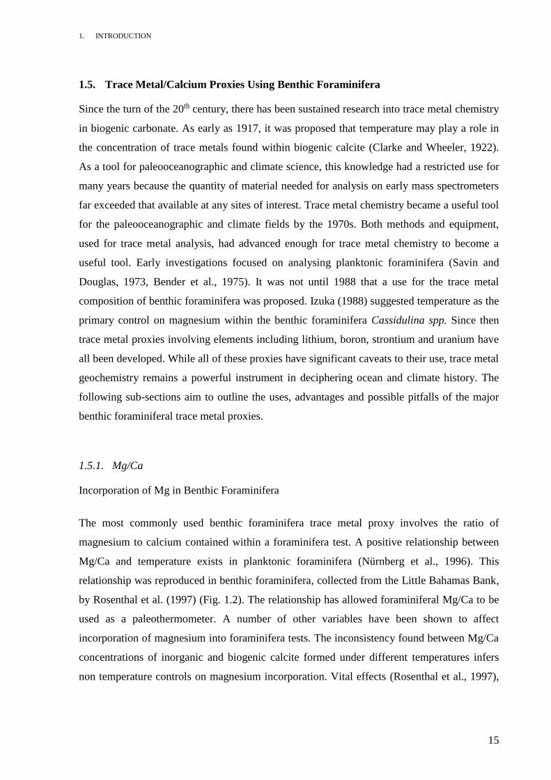
Δ[CO32−] (Martin et al., 2002) and salinity (Ferguson et al., 2008) have all been proposed as

significant variables affecting the ratio of magnesium to calcium in both planktonic and

benthic foraminifera. However, the effect of salinity on benthic foraminifera is yet to be

quantified.

Figure 1.2 Mg/Ca incorporation into the benthic foraminiferal species Cibicidoides

pachyderma (floridanus) as a function of water temperature. The solid line represents an

exponential fit while the dashed lines are a forecast interval at the 96% level from (Rosenthal

et al., 1997).

Limitations

The use of Mg/Ca as a paleothermometer is complicated by a number of factors. Vital effects

specific to individual species of foraminifera have been shown to affect incorporation of

magnesium into the test calcite (Lear et al., 2002). Genetic variability exists between different

foraminifera species. This may account for the differences in magnesium incorporation

observed. However, genetic variability affecting Mg/Ca ratios is yet to be proven. Interspecies

differences in Mg/Ca are corrected for using species specific calibrations.

1. INTRODUCTION

17

Diagenetic processes, the physical and chemical changes that occur after burial, may also

contribute to the concentration of Mg/Ca within each shell. Of note is dissolution, which may

lead to lower mg/ca ratios. Brown and Elderfield (1996) showed that calcite containing more

trace metals dissolved preferentially over pure calcite. The joint processes of neomorphism

and cementation may also alter Mg/Ca ratios. These processes raise Mg/Ca by replacing

biogenic calcite with the inorganic form of the crystal. Inorganic calcite has a higher ratio of

Mg/Ca due to a larger participation coefficient for the magnesium ion (Katz, 1973).

Investigation of deeply buried foraminifera showed only a small increase in Mg/Ca between

poorly and well preserved foraminifera. Therefore, it is likely diagenetic effects can be

disregarded due to their minimal impact.

A salinity related impact on Mg/Ca has been discovered in planktonic foraminifera inhabiting

high salinity areas (Rosenthal et al., 2000). This impact was supported by Ferguson et al.

(2008) who suggested salinity may have significant implications for the interpretation of

downcore records. The effect of salinity on benthic foraminifera is unknown. However, there

is unlikely to be any salinity based effect in low salinity areas.

Changes in the proportion of Mg2+ to Ca2+ in seawater can affect the incorporation magnesium

into a test. There are no direct records of seawater Mg/Ca. This makes indirect evidence vital

to the Mg/Ca paleothermometer. Attempts have been made to ascertain past seawater Mg/Ca

using evaporite fluid inclusions (Lowenstein et al., 2001), Mg/Ca from biogenic carbonates

formed during the greenhouse climates of the early Cenozoic (Lear et al., 2002), models of

processes affecting Mg/Ca in the oceans (Demicco et al., 2005) and calcium carbonate veins

(Coggon et al., 2010). The application of these methods has proved difficult and a large range

of values representing past seawater Mg/Ca have been produced. The relatively long

residence times of Mg2+ and Ca2+ in the ocean (~1 and ~10 Ma respectively) allows

temperature calculations to be relatively accurate despite questions remaining as to the

concentrations in past seawater (Broecker et al., 1982). By adding a seawater concentration

component to Mg/Ca calibration equations the effect of changes is minimised.

The final and largest limitation of using test Mg/Ca as a paleothermometer is saturation state

change. Saturation state change has been offered as a mechanism for Mg/Ca records where

Mg/Ca rises when a fall is expected due to negative temperature change (Coxall et al., 2005).

The saturation state change hypothesis was proposed by Elderfield et al. (2006), who showed

1. INTRODUCTION

18

that the foraminifera Cibicidoides wuellerstorfi has a Mg/Ca sensitivity to saturation state

change of 0.0086 ± 0.0006 mmol/mol/μmol/kg. A higher saturation state increases the ratio of

Mg/Ca within benthic foraminifera. Accurate Mg/Ca paleothermometry requires

quantification of saturation state change in order to be effective. It has been proposed that

where saturation state change cannot be quantified, infaunal species of benthic foraminifera

can be used because they are relatively buffered against saturation state change (Elderfield et

al., 2010).

Calibration

A number of species specific calibrations exist in order to calculate temperature from benthic

foraminiferal Mg/Ca. Using table 1.1 and equation 1.6, bottom water temperature can be

quantified for individual foraminifera species. Almost all benthic Mg/Ca calibrations are

given an exponential fit and therefore use the general equation:

EQN. (1.6)

𝑀𝑔/𝐶𝑎𝐹𝑂𝑅𝐴𝑀 = 𝐵 exp (𝐴 × 𝑇)

where T is temperature. A and B can be found in table 1.1. Lear (2007) proposed the addition

of a past seawater Mg/Ca component to this general equation (Equation 1.7) so as to account

for changes in ocean chemistry.

EQN. (1.7)

𝑀𝑔/𝐶𝑎𝐹𝑂𝑅𝐴𝑀 = 𝑀𝑔/𝐶𝑎𝑠𝑤−𝑇

𝑀𝑔/𝐶𝑎𝑠𝑤−0 × 𝐵 exp (𝐴 × 𝑇)

where sw-0 is modern Mg/Ca in seawater and sw-T is estimated Mg/Ca in seawater for

sample age. When investigating short term shifts in Mg/Ca, past seawater concentrations of

magnesium and calcium are not required due to their reasonably long residence times.

Evidence suggest that early Cenozoic seawater Mg/Ca was not less than two thirds of today’s

value of approximately 5.2 mol/mol (Lear et al., 2002).

Care should be taken because the Mg/Ca of some species has been shown to agree more

readily with a linear fit than an exponential fit (Marchitto et al., 2007). A linear fit produces

unrealistic bottom water temperatures for other species (Lear et al., 2008).

1. INTRODUCTION

19

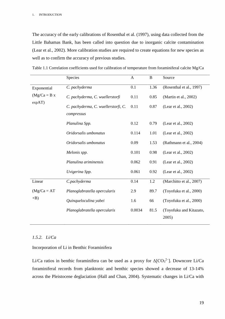
The accuracy of the early calibrations of Rosenthal et al. (1997), using data collected from the

Little Bahamas Bank, has been called into question due to inorganic calcite contamination

(Lear et al., 2002). More calibration studies are required to create equations for new species as

well as to confirm the accuracy of previous studies.

Table 1.1 Correlation coefficients used for calibration of temperature from foraminiferal calcite Mg/Ca

Species A B Source

Exponential

(Mg/Ca = B x

expAT)

C. pachyderma 0.1 1.36 (Rosenthal et al., 1997)

C. pachyderma, C. wuellerstorfi 0.11 0.85 (Martin et al., 2002)

C. pachyderma, C. wuellerstorfi, C.

compressus

0.11 0.87 (Lear et al., 2002)

Planulina Spp. 0.12 0.79 (Lear et al., 2002)

Oridorsalis umbonatus 0.114 1.01 (Lear et al., 2002)

Oridorsalis umbonatus 0.09 1.53 (Rathmann et al., 2004)

Melonis spp. 0.101 0.98 (Lear et al., 2002)

Planulina ariminensis 0.062 0.91 (Lear et al., 2002)

Uvigerina Spp. 0.061 0.92 (Lear et al., 2002)

Linear

(Mg/Ca = AT

+B)

C.pachyderma 0.14 1.2 (Marchitto et al., 2007)

Planoglabratella opercularis 2.9 89.7 (Toyofuku et al., 2000)

Quinqueloculina yabei 1.6 66 (Toyofuku et al., 2000)

Planoglabratella opercularis 0.0034 81.5 (Toyofuku and Kitazato,

2005)

1.5.2. Li/Ca

Incorporation of Li in Benthic Foraminifera

Li/Ca ratios in benthic foraminifera can be used as a proxy for Δ[CO32−]. Downcore Li/Ca

foraminiferal records from planktonic and benthic species showed a decrease of 13-14%

across the Pleistocene deglaciation (Hall and Chan, 2004). Systematic changes in Li/Ca with

1. INTRODUCTION

20

δ18O were too large to be temperature derived alone, another variable must be affecting Li/Ca

(Hall and Chan, 2004). As an alternative, carbonate saturation state has been proposed as the

driver for variability seen in Li/Ca records. A link between benthic foraminiferal Li/Ca and

carbonate saturation state was presented by Lear and Rosenthal (2006) using core top data

from a water depth transect in the Norwegian Sea. This core top data suggests a linear

relationship between Li/Ca and carbonate saturation state (Fig. 1.3). Comparisons between

downcore records and the Van Andel (1975) historic CCD data led to the suggestions that

Li/Ca in benthic foraminifera is dependent on Δ[CO32−] (Lear and Rosenthal, 2006).

Figure 1.3 Record of Li/Ca in the benthic foraminifera Oridorsalis umbonatus, temperature

(thick line) and Δ[CO32−] (thin line) plotted against water depth (boxes) adapted from (Lear

and Rosenthal, 2006). Scatter points represent changing benthic foraminiferal Li/Ca with

water depth.

Limitations

The effectiveness of this proxy is limited by a number of factors. Firstly, the concentration of

Li/Ca in benthic foraminifera has a temperature component. Li/Ca decreases with increasing

temperature (Marriott et al., 2004a, Marriott et al., 2004b). Therefore, any quantification of

changes in Δ[CO32−] requires the temperature component to be calculated using a more

1. INTRODUCTION

21

constrained proxy, such as Mg/Ca. An initial attempt to decipher EOT temperature and

Δ[CO32−] from deep sea benthic foraminiferal Mg/Ca and Li/Ca was presented in Lear et al.

(2010). The attempt was not entirely successful in splitting apart the temperature and

Δ[CO32−] signals, succeeding at some sites but not at others. Secondary effects and calibration

thresholds were proposed as the cause of any failures. Secondly, when applied over periods

longer than 1.5 Ma (the approximate residence time of lithium in the oceans (Huh et al.,

1998)), changes in seawater concentration of lithium/calcium must be considered. A seawater

lithium record covering the past 68 Ma showed an increase of 9 ppm (Misra and Froelich,

2012). This record may be of value with respect to the paired Li/Ca Mg/Ca proxy. Thirdly,

species specific vital effects are known to affect trace metal uptake in benthic foraminifera.

This means species specific calibrations are needed to quantify Δ[CO32−].

Calibration

To date, the only calibration using benthic foraminiferal Li/Ca and Mg/Ca to unravel

Δ[CO32−] uses Oridorsalis umbonatus (Lear et al., 2010). The bottom water Δ[CO3

2−] is

calculated from O. umbonatus Li/Ca and Mg/Ca using the following equation:

EQN. (1.8)

Δ[𝐶𝑂3 2−] =

ΔMg + 0.162ΔLi

0.0162

Using this approach the bottom water Δ[CO32−] can be calculated if the change in magnesium

and lithium are known.

1.5.3. B/Ca

Incorporation of B in Benthic Foraminifera

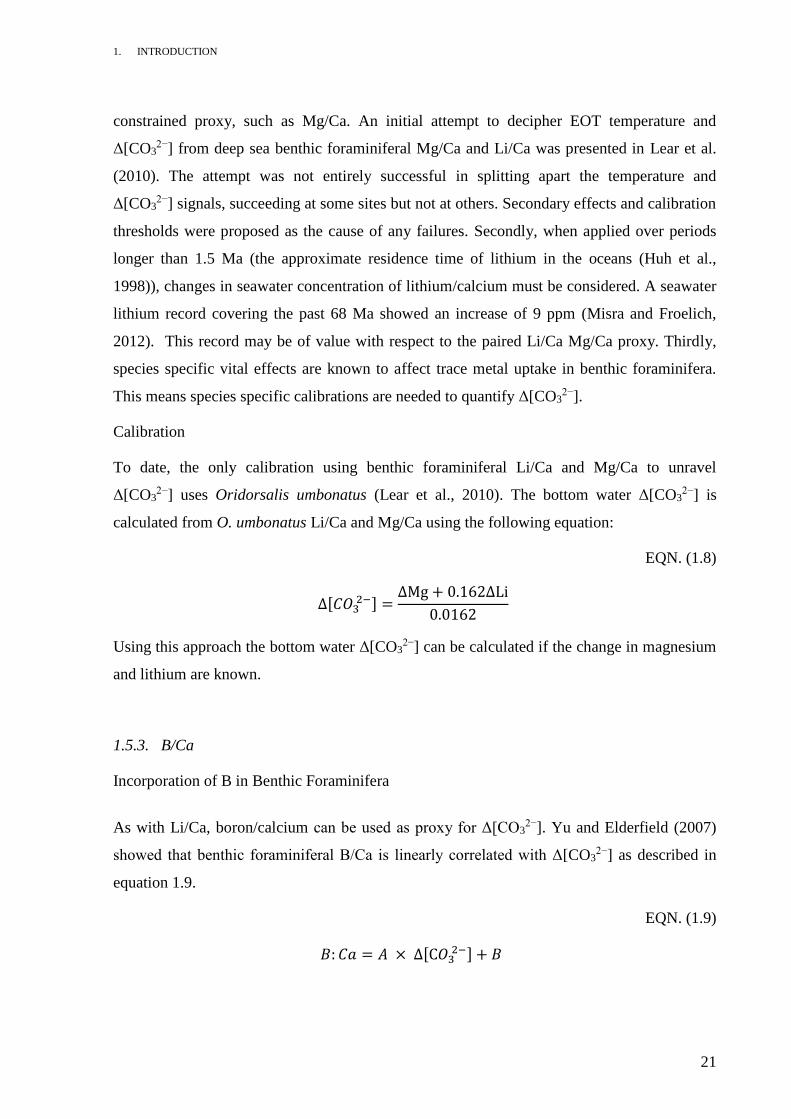
As with Li/Ca, boron/calcium can be used as proxy for Δ[CO32−]. Yu and Elderfield (2007)

showed that benthic foraminiferal B/Ca is linearly correlated with Δ[CO32−] as described in

equation 1.9.

EQN. (1.9)

𝐵: 𝐶𝑎 = 𝐴 × Δ[C𝑂3 2−] + 𝐵

1. INTRODUCTION

22

while values for A and B can be found in table 1.2. The response of epifaunal benthic

foraminiferal B/Ca to Δ[CO32−] is well documented (Yu and Elderfield, 2007, Yu et al., 2010,

Brown et al., 2011). The pore waters, which infaunal species inhabit, are often saturated with

respect to the carbonate ion (Martin and Sayles, 1996). As with infaunal Mg/Ca (Elderfield et

al., 2010), infaunal boron appears to be relatively buffered against Δ[CO32−].

Limitations

As with other foraminiferal trace metal proxies, the usefulness of B/Ca is limited by a number

of factors. Firstly, infaunal B/Ca is expected to be low concentration (Uvigerina spp. B/Ca

∼20 µmol/mol) (Yu and Elderfield, 2007). Therefore, the concentrations recovered may be

under the detection limits of traditional foraminiferal trace metal methodologies. A method

for collecting more precise data has been proposed (Misra et al., 2014). Without such a

method, infaunal B/Ca records are not suitable for analysis. Secondly, concentrations of B/Ca

in the oceans will affect the B/Ca record in foraminiferal calcite. Boron has a long residence

time in the oceans. Lemarchand et al. (2000) calculated a boron residence time of ~14 Ma.

The model presented in Lemarchand et al. (2002) predicts a relatively stable concentration of

oceanic boron across the Cenozoic (~10% variation). Thirdly, species specific vital effects are

known to affect trace metal uptake in benthic foraminifera where there is a large variance in

B/Ca between species. Cases of different B/Ca have been reported between morphotypes of

the same species adding further difficulty when trying to empirically ascertain Δ[CO32−] (Rae

et al., 2011). This means species specific calibrations are needed to quantify Δ[CO32−].

Calibration

Using equation 1.9 and table 1.2, the bottom water Δ[CO32−] can be quantified using

foraminiferal B/Ca. The large range of the coefficients shown in table 1.2 highlights the need

for species specific calibrations. The infaunal species O. umbonatus and Uvigerina spp. have

markedly lower calibration coefficients than the epifaunal species. The B/Ca responses to

Δ[CO32−] for Nuttallides umbonifera and Cibicidoides wuellerstorfi are comparable while the

remaining epifaunal species, Cibicidoides mundulus, has significantly lower coefficients.

1. INTRODUCTION

23

Table 1.2 Correlation coefficients used for calibration of Δ[CO32−] from foraminiferal calcite B/Ca

Species A B Source

Nuttallides umbonifera 1.23 ± 0.15 134 ± 2.7 (Brown et al., 2011)

Cibicidoides wuellerstorfi 1.14 ± 0.048 177.1 ± 1.41 (Yu and Elderfield, 2007)

Cibicidoides mundulus 0.69 ± 0.072 119.1 ± 2.62 (Yu and Elderfield, 2007)

Oridorsalis umbonatus 0.29 ± 0.2 56.4 ± 5.5 (Brown et al., 2011)

Uvigerina spp. 0.27 ± 0.076 19.4 ± 2.99 (Yu and Elderfield, 2007)

1.5.4. Sr/Ca

Incorporation of Sr in Benthic Foraminifera

Another possible proxy for Δ[CO32−] is the Sr/Ca ratio found in foraminifera shells. Core top

studies of benthic foraminiferal Sr/Ca have shown a negative correlation between shell Sr/Ca

and water depth (Rosenthal et al., 1997, Lear et al., 2003, Yu et al., 2014). Unlike B/Ca and

Li/Ca, there no evidence for a temperature component controlling Sr/Ca concentrations in

calcitic benthic foraminifera. The lack of temperature dependency suggests pressure or

Δ[CO32−] is the dominant control on Sr/Ca concentrations in calcitic foraminifera. Strontium

provides a unique record of Δ[CO32−], albeit a limited one.

Limitations

The partitioning of strontium in calcitic foraminifera is poorly understood. It is highly likely

that species specific vital effects play a role in strontium incorporation as with other trace

metal proxies. To ascertain the Δ[CO32−] reliably from foraminiferal Sr/Ca, the past

concentration of strontium in the ocean must be calculated. Using the Sr/Ca record from a

gastropod, Sosdian et al. (2012) calculated past seawater strontium concentration and

suggested that there were minimal variations from the Eocene to the Pliocene.

Calibration

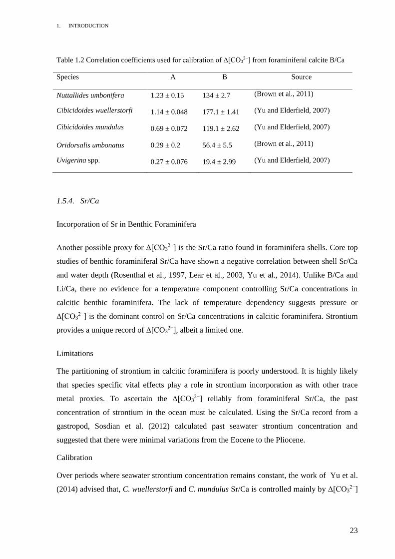
Over periods where seawater strontium concentration remains constant, the work of Yu et al.

(2014) advised that, C. wuellerstorfi and C. mundulus Sr/Ca is controlled mainly by Δ[CO32−]

1. INTRODUCTION

24

(Fig. 1.4). Therefore, Sr/Ca from benthic foraminifera may be used as an auxiliary proxy,

despite no calibration existing to quantify Δ[CO32−].

Figure 1.4 The response of foraminiferal Sr/Ca to deep water Δ[CO32−].

(A) C. wuellerstorfi Sr/Ca and (B) C. mundulus Sr/Ca. Error bars represent ±1σ of

replicates. DSr = (Sr/Ca) shell / (Sr/Ca) seawater. Solid lines in A and B represent the best linear

fits for each data set from (Yu et al., 2014).

1.5.5. U/Ca

Incorporation of U in Benthic Foraminifera

Initial studies of Uranium within benthic foraminifera shells, by Russell et al. (1994),

indicated that U/Ca is controlled by seawater uranium concentration only. Later investigations

showed a marked increase in U/Ca (~25%) from the last glacial period to the Holocene

(Russell et al., 1996). The authors found a correlation between downcore records of U/Ca and

Mg/Ca, this strongly points toward changes in metal incorporation or dissolution as opposed

1. INTRODUCTION

25

to changes in seawater uranium concentration. Anoxic exchange with pore water uranium was

ruled out due to the oxic depositional environment of the studied cores. Dissolution effects are

discounted because well preserved cores with opposite depositional histories show the same

trend. The assumption of temperature as the dominant control on U/Ca in foraminifera is

proposed (Yu et al., 2008). This proposal is supported by the finding that planktonic

foraminiferal U/Ca is inversely proportional to temperature (Yu et al., 2008). Further work by

Russell et al. (2004), with planktonic foraminifera, showed a strong negative correlation

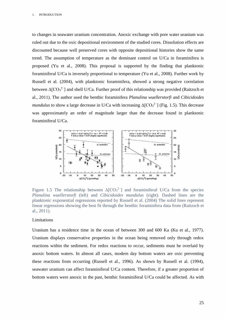
between Δ[CO32−] and shell U/Ca. Further proof of this relationship was provided (Raitzsch et

al., 2011). The author used the benthic foraminifera Planulina wuellerstorfi and Cibicidoides

mundulus to show a large decrease in U/Ca with increasing Δ[CO32−] (Fig. 1.5). This decrease

was approximately an order of magnitude larger than the decrease found in planktonic

foraminiferal U/Ca.

Figure 1.5 The relationship between Δ[CO32−] and foraminiferal U/Ca from the species

Planulina wuellerstorfi (left) and Cibicidoides mundulus (right). Dashed lines are the

planktonic exponential regressions reported by Russell et al. (2004) The solid lines represent

linear regressions showing the best fit through the benthic foraminifera data from (Raitzsch et

al., 2011).

Limitations

Uranium has a residence time in the ocean of between 300 and 600 Ka (Ku et al., 1977).

Uranium displays conservative properties in the ocean being removed only through redox

reactions within the sediment. For redox reactions to occur, sediments must be overlaid by

anoxic bottom waters. In almost all cases, modern day bottom waters are oxic preventing

these reactions from occurring (Russell et al., 1996). As shown by Russell et al. (1994),

seawater uranium can affect foraminiferal U/Ca content. Therefore, if a greater proportion of

bottom waters were anoxic in the past, benthic foraminiferal U/Ca could be affected. As with

1. INTRODUCTION

26

all of the discussed trace metal proxies, there appears to be significant inter species vital

effects controlling incorporation of uranium into foraminifera. This can be resolved by using

species specific calibrations. However few of these currently exist.

Calibration

P. wuellerstorfi and C. mundulus U/Ca is mainly controlled by Δ[CO32−] (Raitzsch et al.,

2011). The authors believe that any correlation with temperature, as shown empirically by Yu

et al. (2008), is due to the relationship between temperature and Δ[CO32−], suggesting that

temperature is not a direct control on U/Ca in benthic foraminifera. Therefore, Raitzsch et al.

(2011) proposed the following linear equation as a suitable calibration of Δ[CO32−] from

U/Ca:

EQN. (1.10)

𝑈: 𝐶𝑎 = 𝐴 × Δ[C𝑂3 2−] + 𝐵

Table 1.3 contains the species specific correlation coefficients for use with equation 1.10

when calculating Δ[CO32−] from benthic foraminiferal U/Ca.

Table 1.3 Correlation coefficients used for calibration of Δ[CO32−] from foraminiferal calcite

U/Ca

Species A B Source

Planulina wuellerstorfi -0.27 ± 0.04 15.1 ± 1.4 (Raitzsch et al., 2011)

Cibicidoides mundulus -0.30 ± 0.06 14.6 ± 1.8 (Raitzsch et al., 2011)

1. INTRODUCTION

27

1.6. Eocene-Oligocene Transition

The Eocene-Oligocene (E-O) boundary (~34 Ma) is known as Earth’s greenhouse-icehouse

transition (Francis et al., 2008). During the Eocene-Oligocene transition (EOT), the first

Cenozoic ice sheets appeared on the Antarctic continent (Kennett and Shackleton, 1976). The

Eastern Antarctic continent was entirely buried under ice by the onset of the Oligocene

(Ehrmann and Mackensen, 1992). After decades of study, terminology associated with the

EOT has become confused. The terminology used here follows that presented in Lear et al.

(2008). The E-O boundary is formally identified by the extinction event associated with the

planktonic foraminiferal family Hankeninidae (Coccioni et al., 1988).

1.6.1. Oxygen Stable Isotope Records

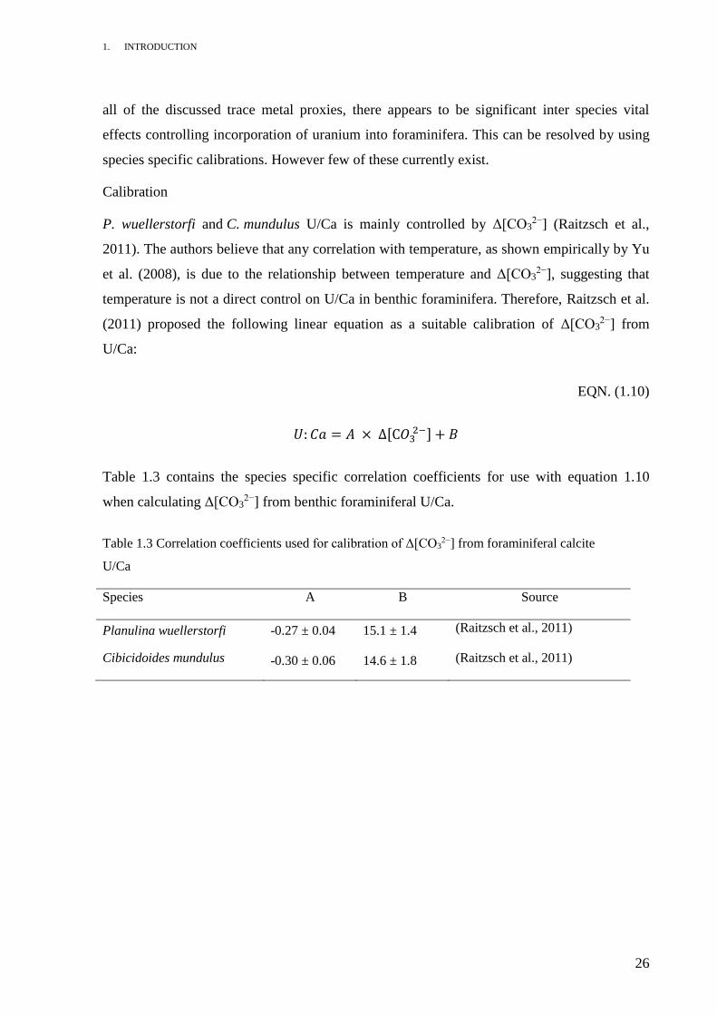
A geochemical signal exists recording the EOT. Two shifts exist in deep water foraminiferal

oxygen isotope values (δ18O), Oligocene isotope shift 1 (Oi-1) (termed here as Step 2),

represents the shift to maximum values of δ18O at the Early Oligocene Glacial Maximum

(EOGM) while a precursor shift , termed here as Step 1, is also observed (Fig. 1.6a) (Coxall et

al., 2005). Coxall et al. (2005) noted that the oxygen isotope shifts Step 1 and Step 2

coincided with a ~1 km deepening of the carbonate compensation depth (CCD) discovered by

Van Andel (1975) (Fig. 1.6b).

Figure 1.6(a) high-resolution data from ODP site 1218 showing a stepwise δ18O increase in

benthic foraminiferal calcite and (b) published CCD data from Deep Sea Drilling Program

(DSDP) sites across the last 50 Ma (Van Andel, 1975). The figure shows a ~1 km deepening

of the CCD at the E-O boundary (timing and duration of the shift is poorly constrained). The

shaded bar represents an uncertainty of ~3 Ma adapted from (Coxall et al., 2005).

Step 2 Step 1

(a) (b)

δ18

O (‰ VPDB)

1. INTRODUCTION

28

The ~1 km deepening of the CCD is associated with the drawdown of atmospheric carbon

dioxide (CO2atm). The magnitude of this drawdown (~25 µatm) is unlikely large enough to

initiate large scale glaciation of Antarctica (Sigman and Boyle, 2000). It appears more likely

that the increase in CCD is glaciation related. One theory is that the availability of continental

shelf (where neritic benthic calcifiers are found) decreased upon glaciation of Antarctica,

which shifted CaCO3 deposition into the pelagic deep sea realm from the benthic neritic realm

(James, 1978, Merico et al., 2008).

1.6.2. Trace Metal Records

The size of shift in the δ18O record is not accounted for by Antarctic glaciation. Either

significant Northern Hemisphere ice accumulation was occurring concurrently with Antarctic

glaciation or there was a temperature component to the δ18O shift. Climate modelling does not

support Northern Hemisphere ice growth across the EOT (Deconto et al., 2008), although

some minor glaciation has been discovered on Greenland during the period (Eldrett et al.,

2007). For bipolar glaciation to occur, the models of Deconto et al. (2008) predict a much

lower PCO2atm than occurred at the EOT. Therefore, it follows that a significant cooling event

impacted upon records of δ18O during the EOT.

Concentration of magnesium with respect to calcium is known to be temperature dependant,

with increased magnesium calcium representing increasing temperature (Burton and Walter,

1991). Foraminiferal Mg/Ca can therefore be used as a paleothermometer. This enables the

temperature and δ18OSW components of δ18O to be separated. Using foraminiferal Mg/Ca

ratios from very well preserved Tanzanian foraminifera deposited well above the CCD, it has

been indicated that Step 1 was predominantly associated with cooling global temperatures

(~2.5⁰C) (Lear et al., 2008), while Step 2 was linked to rapid ice growth and sea level decline

(Coxall et al., 2005). Microfacies, sedimentological and biotic analysis also confirm the

existence of a coupled cooling and ice growth stimulus for initial changes in δ18O with no

sustained cooling associated with Step 2 (Houben et al., 2012). The cooling trend at the first

isotope shift is supported by planktonic foraminiferal Mg/Ca proxy information from ODP

sites 738, 744, and 748 (the Kerguelen Plateau) (Bohaty et al., 2012). However the cooling

event is not observed in benthic foraminiferal Mg/Ca ratios at the same sites.

1. INTRODUCTION

29

Early attempts to apply Mg/Ca paleothermometry to the EOT also supplied no evidence of a

cooling trend from the Eocene to the Oligocene (Lear et al., 2004, Lear et al., 2000, Billups

and Schrag, 2003), while the record at ODP Site 1218 showed a slight increase in temperature

(Lear et al., 2004). One explanation for this relates to the concurrent deepening of the CCD. A

Δ[CO32−] effect is able to affect Mg/Ca records (Elderfield et al., 2006). By quantifying

Δ[CO32−], Lear et al. (2010) corrected the temperature records presented for DSDP Site 522

and ODP Site 1218 (Lear et al., 2004, Lear et al., 2000). After Δ[CO32−] correction, cooling

was shown across the EOT at these sites. Three methods have been proposed to correct for

Δ[CO32−] effect (1) the use of ostracod Mg/Ca because these appear unaffected by Δ[CO3

2−]

(Dwyer et al., 2002), (2) correction of benthic foraminiferal Mg/Ca records using B/Ca or

Li/Ca proxies (used to calculate Δ[CO32−]) (Yu and Elderfield, 2007, Lear and Rosenthal,

2006, Lear et al., 2010) and (3) use of infaunal benthic foraminiferal Mg/Ca ratios as these are

potentially buffered against any change in Δ[CO32−] (Elderfield et al., 2010). Poor proxy

resolution or complications regarding Mg/Ca paleothermometry at low temperatures may also

explain these results.

1.6.3. Proposed Mechanisms for EOT Initiation

The cause of the EOT is unknown. Theories include: declining PCO2atm

levels (Deconto and

Pollard, 2003), the opening of gateways around Antarctica enabling the formation of the

Antarctic Circumpolar Current (ACC), which subsequently thermally isolated the continent

(Toggweiler and Bjornsson, 2000) and increased upwelling of warm water, which promoted

the transport of moisture across the already cold continent, initiating ice expansion (Prentice

and Matthews, 1991). The establishment of the ACC at this time has also been linked to

changing nutrient concentrations in the ocean (Egan et al., 2013, Scher and Martin, 2006). If

the altered nutrient system increased carbon export to the sediments then this may explain the

decreasing PCO2atm proposed by Deconto and Pollard (2003). It has, however, been

postulated that the opening of gateways had a less significant impact on water mass

circulation change than has been reported previously. It was shown that ice sheet growth and

not the establishment of the ACC caused increased transport northward of Antarctic

intermediate water, stimulating the formation of Antarctic bottom water (Goldner et al.,

2014). This evidence supports declining PCO2 across the EOT as the driver for ice sheet

growth rather than the proposed circulation change created by the establishment of the ACC.

1. INTRODUCTION

30

Geochemical proxy data, from very well preserved foraminifera collected by the Tanzanian

Drilling Project, also supports the Deconto and Pollard (2003) model’s assumption that

declining PCO2atm

is central to the expansion of the Antarctic ice sheet (Pearson et al., 2009).

The reality is that initiation of EOT ice sheet expansion is poorly constrained and glaciation of

Antarctica could be a response to any of the proposed mechanisms.

1. INTRODUCTION

31

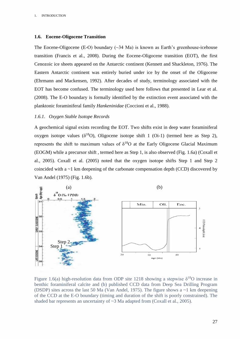
1.7. Regional and Geological Setting

The microfossil material analysed in this study was recovered from ODP Hole 757B, which

currently lies upon the Ninety East Ridge, in a water depth of 1644 m (17°01.458'S,

88°10.899'E) (Fig. 1.7a) (Peirce et al., 1989). Analysed core sections ranged between 13H-1

(5-7 cm) and 14H-cc (6-8 cm). During the EOT, the site was ~13°S of its current position

(Fig. 1.7b). Preservation of foraminifera was reported as being good to moderate by the

shipboard scientific party (Peirce et al., 1989). The shipboard party also reported a paleo

water depth of ~1500 m, for the samples under investigation in this study. This paleo water

depth is well above the Eocene and Oligocene paleo CCDs of 3400 m and 4400 m (Van

Andel, 1975).

Figure 1.7 (a) the current positions of ODP Holes 757B and 763A within the Indian Ocean

and (b) a paleo reconstruction of the same sites at 33.9 million years before present plotted

using the ODSN advanced plate reconstruction tool (Hay, 2000).

(a)

(b)

1. INTRODUCTION

32

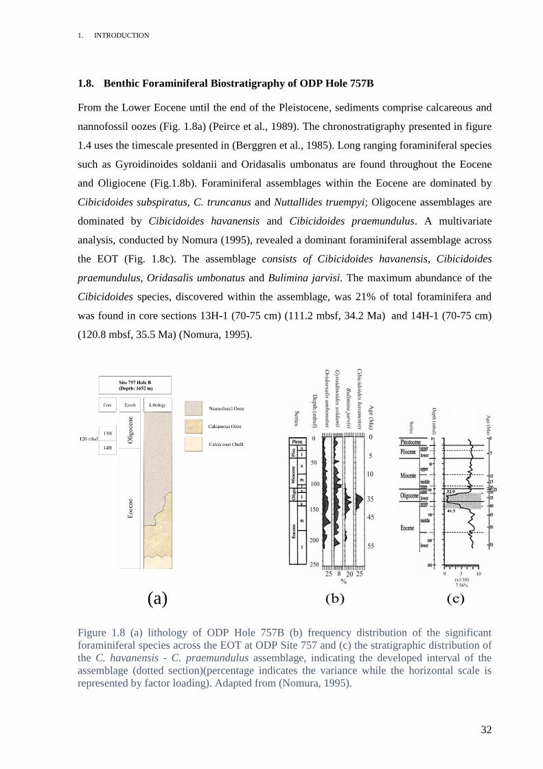
1.8. Benthic Foraminiferal Biostratigraphy of ODP Hole 757B

From the Lower Eocene until the end of the Pleistocene, sediments comprise calcareous and

nannofossil oozes (Fig. 1.8a) (Peirce et al., 1989). The chronostratigraphy presented in figure

1.4 uses the timescale presented in (Berggren et al., 1985). Long ranging foraminiferal species

such as Gyroidinoides soldanii and Oridasalis umbonatus are found throughout the Eocene

and Oligiocene (Fig.1.8b). Foraminiferal assemblages within the Eocene are dominated by

Cibicidoides subspiratus, C. truncanus and Nuttallides truempyi; Oligocene assemblages are

dominated by Cibicidoides havanensis and Cibicidoides praemundulus. A multivariate

analysis, conducted by Nomura (1995), revealed a dominant foraminiferal assemblage across

the EOT (Fig. 1.8c). The assemblage consists of Cibicidoides havanensis, Cibicidoides

praemundulus, Oridasalis umbonatus and Bulimina jarvisi. The maximum abundance of the

Cibicidoides species, discovered within the assemblage, was 21% of total foraminifera and

was found in core sections 13H-1 (70-75 cm) (111.2 mbsf, 34.2 Ma) and 14H-1 (70-75 cm)

(120.8 mbsf, 35.5 Ma) (Nomura, 1995).

Figure 1.8 (a) lithology of ODP Hole 757B (b) frequency distribution of the significant

foraminiferal species across the EOT at ODP Site 757 and (c) the stratigraphic distribution of

the C. havanensis - C. praemundulus assemblage, indicating the developed interval of the

assemblage (dotted section)(percentage indicates the variance while the horizontal scale is

represented by factor loading). Adapted from (Nomura, 1995).

(a)

1. INTRODUCTION

33

1.9. Pilot Ostracod Study

A Cardiff Undergraduate Research Opportunities Programme (CUROP) funded project was

completed by the author in 2014. It investigated the Mg/Ca ratio in the deep-sea ostracod

genus Krithe at ODP Site 757. The aim of this project was to create an EOT Mg/Ca record

unaffected by Δ[CO32−]. Ostracods are a type of bi-valved crustacean predominantly formed

from the calcium carbonate (CaCO3) polymorph calcite (Fig. 1.9). They contain co-

precipitated magnesium similar to foraminifera. Due to ostracod’s infaunal habitat, it has been

proposed that they are relatively buffered against Δ[CO32−] (Dwyer et al., 2002).

Figure 1.9 Light micrographs of Krithe spp. recovered from ODP Hole 757B Core 14 Section

1 44-46 cm.

A Δ[CO32−] effect on calcitic Mg/Ca is expected across the EOT, at Site 757, because of the

predicted ~1km deepening of the CCD. Concurrent with the CCD deepening, foraminiferal

δ18O shifts at ODP site 757 (Holmström, 2014). The two isotope shifts observed at ODP Site

757 can also be seen in the isotope record of ODP Site 1218 (Fig. 1.10) (Coxall et al., 2005).

For the shifts shown at the two sites, discrepancies between the ages are due to differing age

model methodologies.

An increase in Krithe Mg/Ca was observed across the Eocene/Oligocene boundary at ODP

site 757 (Fig. 1.11). This increase was also observed in Krithe collected from ODP Site 763

(S. Bohaty, pers. comm., 2014). The offset in Mg/Ca between the two sites may be due to

1. INTRODUCTION

34

vital effects affecting different Krithe species or differing depths of the sites. The increase in

Mg/Ca may have been caused by: temperature increase across the EOT, a seawater Mg/Ca

change or a Δ[CO32−] effect on ostracods. A saturation state effect is contrary to the findings

of Dwyer et al. (2002).

It has been demonstrated that the assumption of no carbonate ion effect on ostracods is

incorrect at low temperatures (Elmore et al., 2012). The data from ODP Sites 757 and 763

supports the conclusions presented by Elmore et al. (2012).

Figure 1.10 the oxygen isotope records for ODP Sites 757 (red) and 1218 (blue). Site 757 data

was produced by Holmström (2014) and plotted against the ages calculated by Schedwin

(2014), which used the Geomagnetic Polarity Timescale presented in Wade et al. (2011). The

record from ODP Site 1218 was published by Coxall et al. (2005) and used an astronomical

timescale. The dashed line represents the EO boundary (33.7 Ma) as defined in Wade et al.

(2011). Two isotopic shifts are observed in both records, Step 1 and Step 2.

Step 2

Step 1

1. INTRODUCTION

35

Figure 1.11 Mg/Ca ratios from the Ostracod genus Krithe from ODP Hole 757B (black) and

763A (blue) (Bohaty, 2014) and δ18O from the benthic foraminifera Cibicidoides havanensis

also from ODP Hole 757B (red) (Holmström, 2014). Orange shading represents the predicted

location of Step 1 (right) and Step 2 (left). The dashed line represents the Eocene–Oligocene

transition as defined by the Hantkeninia extinction event. Ages for Site 763 data were

formulated using the GTS2012 geological timescale.

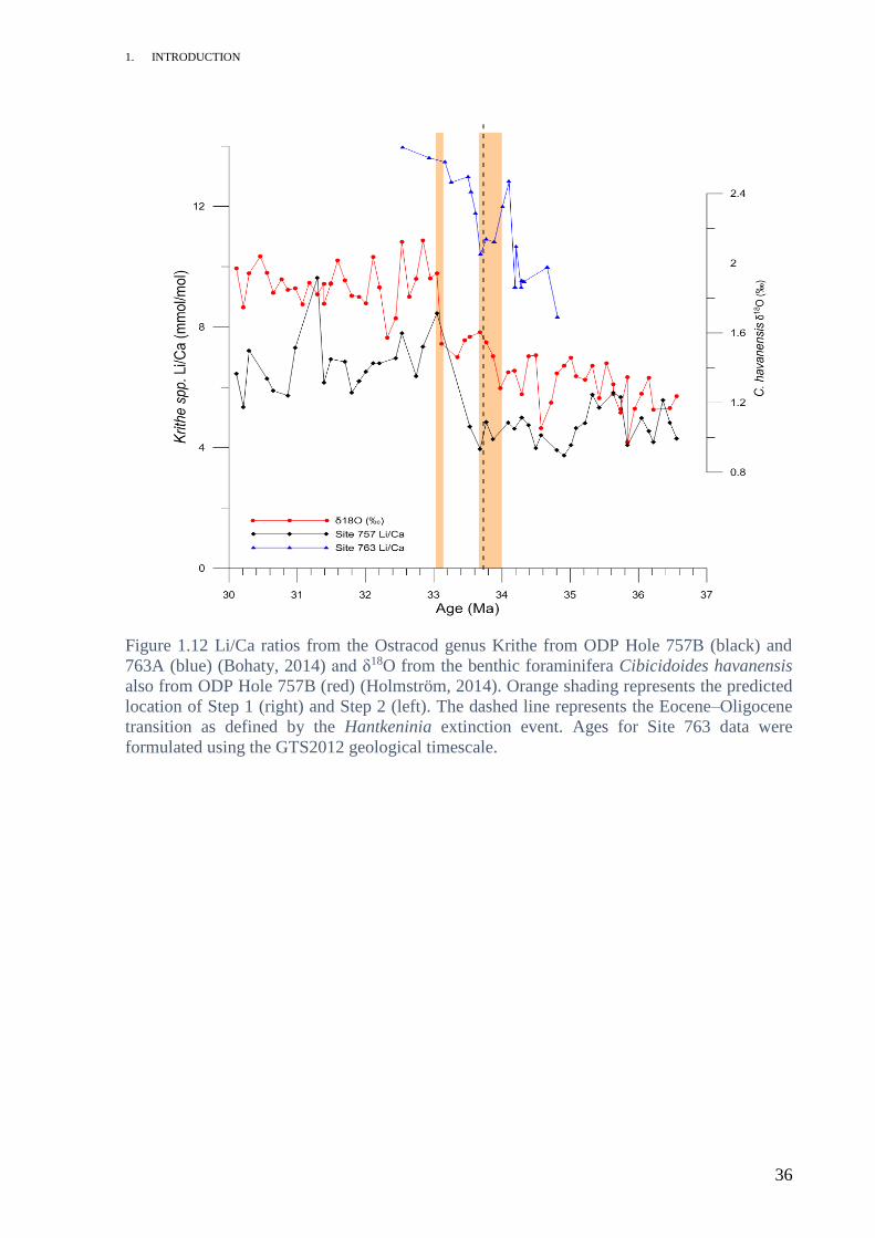
The large increases observed in Li/Ca within the ostracods at the study sites provide further

support for a saturation state effect (Fig. 1.12). Ostracodal Li/Ca was investigated at ODP

Sites 757 and 763. While the environmental controls on lithium incorporation into marine

ostracods are relatively unknown, it is possible to make some assumptions. Lacustrine

ostracodal Li/Ca is temperature dependant similar to benthic foraminiferal Li/Ca (Zhu et al.,

2012). It is safe to assume that temperature and saturation state have the same relationship

with marine ostracodal Li/Ca as they do with that of foraminiferal Li/Ca because both marine

ostracods and foraminifera are formed from calcite. The Li/Ca shift observed could also be

explained by the expected drop in bottom water temperature; Li/Ca has an inverse relationship

with temperature. It is however more likely the shift was caused by a mixture of the two.

1. INTRODUCTION

36

Figure 1.12 Li/Ca ratios from the Ostracod genus Krithe from ODP Hole 757B (black) and

763A (blue) (Bohaty, 2014) and δ18O from the benthic foraminifera Cibicidoides havanensis

also from ODP Hole 757B (red) (Holmström, 2014). Orange shading represents the predicted

location of Step 1 (right) and Step 2 (left). The dashed line represents the Eocene–Oligocene

transition as defined by the Hantkeninia extinction event. Ages for Site 763 data were

formulated using the GTS2012 geological timescale.

1. INTRODUCTION

37

1.10. Motivation

By unravelling the saturation state effect, it is hoped, the climate conditions that occurred

during the EOT can be determined. As discussed, ODP site 757 contains both infaunal and

epifaunal benthic foraminifera. The opportunity to analyse both at the same site is not

common. By comparing both infaunal and epifaunal foraminiferal chemical composition,

changes in water column chemistry can be quantified. The difference in Mg/Ca between

infaunal and epifaunal species may record the effect of saturation state change on the

foraminiferal Mg/Ca because infaunal species are relatively buffered against bottom water

Δ[CO32−] change (Elderfield et al., 2010). Hence, the difference in Mg/Ca can be used to

correct Mg/Ca for Δ[CO32−] change. If infaunal and epifaunal foraminifera records are the

same then Δ[CO32−] change is not responsible for heightened Mg/Ca records in the ostracod

records at ODP Sites 757 and 763. The Li/Ca and B/Ca ratios, from foraminifera at ODP site

757, can be used also to calculate saturation state change.

1.10.1. Hypothesis

A cooling effect is expected as Antarctica becomes glaciated. Consistently, benthic

foraminiferal records show an increase in Mg/Ca during this event and it has been proposed

that a carbonate saturation state effect may play a role (Lear et al., 2004, Elderfield et al.,

2006). It is hypothesised here that saturation state change is responsible for heightened

ostracodal and foraminiferal Mg/Ca ratios found across the Eocene/Oligocene boundary and

not increasing temperature or changing sea water Mg/Ca. A cooling effect associated with the

EOT glaciation of Antarctica rules out temperature increase, while the long residence times of

Mg2+ (~1 Ma) and Ca2+ (~10 Ma) in the ocean (Broecker et al., 1982) make changing seawater

Mg/Ca a less likely driver of rising foraminiferal Mg/Ca than saturation state change. The

consequence of proving this hypothesis is the ability to correct Mg/Ca records for Δ[CO32−]

effect and thus calculate accurate paleo-temperatures and ice volumes for the EOT.

It is predicted that the infaunal benthic Mg/Ca record collected by this study will be buffered

against saturation state change and therefore will not display an increase in Mg/Ca. It is

expected also that the epifaunal benthic B/Ca will show a marked increase across the EOT

while Li/Ca may also increase. Epifaunal benthic foraminiferal U/Ca is predicted to decrease.

Benthic foraminiferal test mass is anticipated to increase due to higher calcification rates

1. INTRODUCTION

38

associated with the deepening CCD. Infaunal test mass is predicted to increase less than

epifaunal mass across the EOT due to the buffering associated with the infaunal micro habitat.

2. MATERIALS AND METHODS

39


Sampling

Microscopy

Weighing

Sample preparation and chemical cleaning

Trace metal analysis

Age model

Calculation of temperature, saturation state and ice volume


40

2.1. Sampling

Cores were recovered in 1989 by the JOIDES Resolution deep sea drilling ship (operated by

the ODP) (Fig 2.1). The coarse fraction of the core collected from ODP Hole 757B was made

available from 110.55 to 129.54 metres below sea floor (mbsf). The coarse fraction contained

all material >63 µm diameter between these depths. The course fraction recovered from 63

intervals, each 2 cm of depth, was provided for this study. The intervals were spread

intermittently across the depth range. The coarse fraction was obtained by washing and

sieving the core in 15.0 MΩ deionized (DI) water (Fig. 2.1). Each sample was viewed under

two times magnification using a Nikon SM7645 light-microscope. All benthic foraminifera

tests were removed from the 250-500 µm size fraction (obtained through sieving the course

fraction) using a fine paintbrush and 15.0 MΩ DI water (Fig 2.1). Next, tests of dominant

benthic foraminifera species (Bulimina jarvisi, Cibicidoides havanensis, Gyroidinoides

soldani and Oridorsalis umbonatus) were removed. Tests with significant dissolution or

discolouring were disregarded. Picked tests with irregular morphological features (such as

size, shape or chamber composition) were disregarded also. Where this was not possible, a

record of any test abnormalities was made.

2.1.1. Species Selection

B. jarvisi and C. havanensis were chosen for trace metal analysis because of their dominance

within the core’s foraminiferal assemblage, as well as the need for an infaunal and epifaunal

species. B. jarvisi is also suitable as it is a relatively deep dwelling infaunal species and may

be more buffered against Δ[CO32−] than a shallower dwelling infaunal species. B. jarvisi tests

were picked from the 250-355 µm size fraction while C. havanensis tests were picked from

the 250-500 µm size fraction.

2.2. Microscopy

Light micrographs of the two species used for geochemical analysis, B. jarvisi and C.

havanensis, were taken. Species were cleaned of any obvious debris before reflected light

microscopy. Relatively well preserved specimens were chosen for this purpose. Images were

taking using a multifocus (montage) method on a Leica MZ16 stereo microscope using

Cardiff University Earth Microscope Computer 1.


41

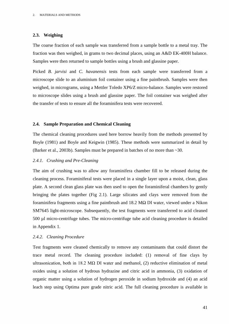
2.3. Weighing

The coarse fraction of each sample was transferred from a sample bottle to a metal tray. The

fraction was then weighed, in grams to two decimal places, using an A&D EK-400H balance.

Samples were then returned to sample bottles using a brush and glassine paper.

Picked B. jarvisi and C. havanensis tests from each sample were transferred from a

microscope slide to an aluminium foil container using a fine paintbrush. Samples were then

weighed, in micrograms, using a Mettler Toledo XP6/Z micro-balance. Samples were restored

to microscope slides using a brush and glassine paper. The foil container was weighed after

the transfer of tests to ensure all the foraminifera tests were recovered.

2.4. Sample Preparation and Chemical Cleaning

The chemical cleaning procedures used here borrow heavily from the methods presented by

Boyle (1981) and Boyle and Keigwin (1985). These methods were summarized in detail by

(Barker et al., 2003b). Samples must be prepared in batches of no more than ~30.

2.4.1. Crushing and Pre-Cleaning

The aim of crushing was to allow any foraminifera chamber fill to be released during the

cleaning process. Foraminiferal tests were placed in a single layer upon a moist, clean, glass

plate. A second clean glass plate was then used to open the foraminiferal chambers by gently

bringing the plates together (Fig 2.1). Large silicates and clays were removed from the

foraminifera fragments using a fine paintbrush and 18.2 MΩ DI water, viewed under a Nikon

SM7645 light-microscope. Subsequently, the test fragments were transferred to acid cleaned

500 µl micro-centrifuge tubes. The micro-centrifuge tube acid cleaning procedure is detailed

in Appendix 1.

2.4.2. Cleaning Procedure

Test fragments were cleaned chemically to remove any contaminants that could distort the

trace metal record. The cleaning procedure included: (1) removal of fine clays by

ultrasonication, both in 18.2 MΩ DI water and methanol, (2) reductive elimination of metal

oxides using a solution of hydrous hydrazine and citric acid in ammonia, (3) oxidation of

organic matter using a solution of hydrogen peroxide in sodium hydroxide and (4) an acid

leach step using Optima pure grade nitric acid. The full cleaning procedure is available in


42

Appendix 2. Additionally, after the clay removal step, any obviously non-carbonate particles

were removed from samples viewed under a Nikon SM7645 light-microscope, 18.2 MΩ DI

water and a fine paintbrush. Reagents used were trace metal grade, unless otherwise stated.


43

Figure 2.1 Sample recovery and analysis. Clockwise from top left: Drill Ship JOIDES

Resolution used to recover cores on ODP Leg 121 from (Crawford, 2013), sample washing

using a 63 µm sieve, glass slides and microscope used during the crushing procedure, Thermo

Finnegan XR high resolution-inductively coupled plasma-mass spectrometer used for trace

metal analysis, chemical cleaning and benthic foraminifera picking using a fine brush and

light microscope.


44

2.5. Sample Dissolution and Calcium Concentration Analysis

One day in advance of trace metal analysis, each sample was dissolved in Optima grade nitric

acid. The full dissolution procedure is available in Appendix 3. Two aliquots, one 10 µl, the

other 100 µl, were removed from each solution and placed in new, acid cleaned tubes. The

smaller of the two aliquots was used to ascertain the calcium concentration ([Ca]) within the

samples while the larger was used to determine trace metal ratios.

Each sample was diluted with Optima grade nitric acid. The [Ca] of each sample was

analysed using a Thermo Element XR high resolution inductively coupled plasma mass

spectrometer (HR-ICP-MS). The [Ca] of each sample was quantified by comparing drift and

blank corrected intensity data (in counts per second of Ca43) to that of a standard containing

80 ppm calcium. Samples were loaded in blocks of five, separated by a blank and a standard

(24 mmol mixed calibration standard, MCS) (Fig. 2.2). A detailed methodology for calcium

concentration analysis is available in Appendix 3.

2.6. Trace Metal Analysis

On the day of trace metal analysis by the HR-ICP-MS, each sample was diluted using Optima

grade nitric acid. Samples were analysed using a Thermo Element XR HR-ICP-MS.

Independent consistency standards (CS1 and CS2) were analysed alongside the MCS at the

start and end of each run. This allowed the long term accuracy and precision of the run to be

quantified. Optima grade nitric acid blanks were analysed after every 2 samples. Matrix

matched standards (MMS) were created using Optima grade nitric acid diluted MCS. The

MMS provided a standard with similar [Ca] for each individual sample. Each MMS was run

directly after its corresponding sample and was used as a barometer for the count accuracy of

the mass spectrometer during the run (Fig. 2.2). This method accounts for the normal

variation in matrix effects observed better than a single matrix effect correction (Lear et al.,

2002). Full elemental analysis included measuring intensities of 6Li, 7Li, 11B, 24Mg, 25Mg,

27Al, 43Ca, 46Ca, 48Ca, 47Ti, 55Mn, 87Sr, 88Sr, 111Cd, 138Ba, 146Nd and 238U. Each

isotope count was blank corrected using the previous blank in the run sequence. A blank

corrected intensity ratio was calculated using the Ca43 intensity and the blank corrected count

for each isotope. An elemental ratio was subsequently formulated using the MMS and the

blank corrected intensity ratios.


45

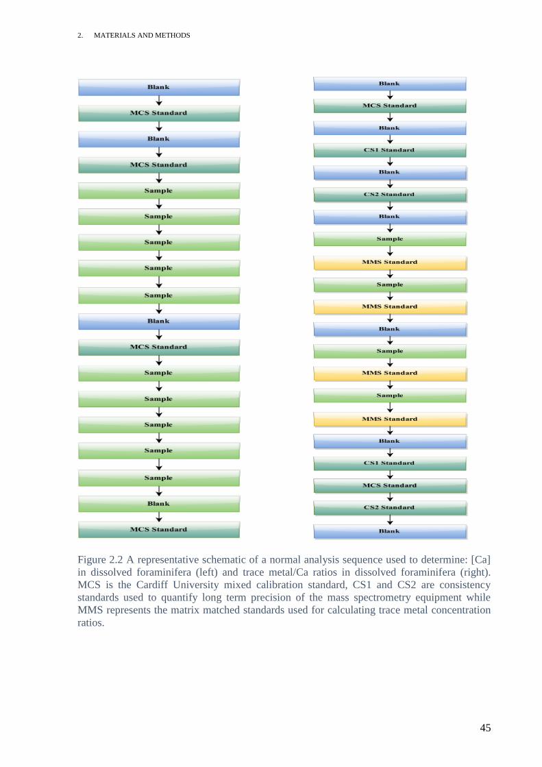
Figure 2.2 A representative schematic of a normal analysis sequence used to determine: [Ca]

in dissolved foraminifera (left) and trace metal/Ca ratios in dissolved foraminifera (right).

MCS is the Cardiff University mixed calibration standard, CS1 and CS2 are consistency

standards used to quantify long term precision of the mass spectrometry equipment while

MMS represents the matrix matched standards used for calculating trace metal concentration

ratios.


46

2.7. Age Model

The age model (Fig. 2.3) which was formulated by Schedwin (2014) using the planktonic

foraminiferal and nannofossil biostratigraphy recorded by the shipboard scientific party of

ODP Leg 121 was applied to the samples analysed in this study (Peirce et al., 1989). The

model utilises the revised geomagnetic polarity time scale (GPTS) presented in Wade et al.

(2011). By measuring the midpoint depth (mbsf) of the samples that correlated with the

nannofossil and planktonic foraminiferal datums, a calibration equation was created allowing

for interpolation within the spread of datum events. A sedimentation rate of 2.9 m/Ma was

predicted for site 757B using the model (Schedwin, 2014).

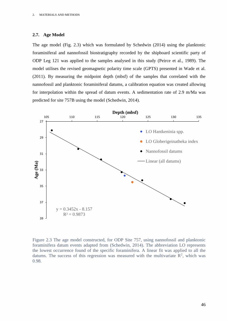
Figure 2.3 The age model constructed, for ODP Site 757, using nannofossil and planktonic

foraminifera datum events adapted from (Schedwin, 2014). The abbreviation LO represents

the lowest occurrence found of the specific foraminifera. A linear fit was applied to all the

datums. The success of this regression was measured with the multivariate R2, which was

0.98.

y = 0.3452x - 8.157

R² = 0.9873

27

29

31

33

35

37

39

105 110 115 120 125 130 135

Age

(Ma)

Depth (mbsf)

LO Hantkeninia spp.

LO Globerigeinatheka index

Nannofossil datums

Linear (all datums)


47

2.8. Calculation of Temperature, Saturation State and Ice Volume

Changes in temperature, saturation state and ice volume can be calculated from raw trace

metal data using a number of calibrations. Listed here are those calibrations that were applied

to the data collected throughout this study. Each calibration was chosen to best match the

species and data under investigation.

Bottom water temperature (T) was calculated from the Mg/Ca of B. jarvisi through the

following equation:

EQN. (2.1)

𝑀𝑔/𝐶𝑎𝐵. 𝑗𝑎𝑟𝑣𝑖𝑠𝑖 = 1.008 exp (0.114 × 𝑇)

(Lear et al., 2002)

The calibration presented in equation 2.1 was derived for the infaunal foraminifera species O.

umbonatus. O. umbonatus have a higher concentration of Mg/Ca than Cibicidoides spp.

Uvigerina spp. is a second infaunal genera for which a temperature calibration exists.

Uvigerina have lower concentrations of Mg/Ca than Cibicidoides (Lear et al., 2002).

Cibicidoides havanensis was shown, by this study, to have a significantly lower Mg/Ca

concentration than B. jarvisi. Therefore, a calibration using the infaunal species O. umbonatus

was chosen because the calibration better fits the data collected.

A first order approximation of early Cenozoic (~49 Ma) Mg/Ca in seawater is 3.5 mol mol-1

while modern concentrations of Mg/Ca in the oceans was measured at approximately 5.2 mol

mol-1. This was combined into equation 2.1 so as to account for changes in oceanic Mg/Ca

from the Eocene to present (Equation 2.2).

EQN. (2.2)

𝑀𝑔/𝐶𝑎𝐵. 𝑗𝑎𝑟𝑣𝑖𝑠𝑖 =3.5

5.2 × 1.008 exp (0.114 × 𝑇)

(Lear et al., 2002)

Saturation state was calculated from the B/Ca of C. havanensis through the following

equation:


48

EQN. (2.3)

𝐵/𝐶𝑎𝐶. ℎ𝑎𝑣𝑎𝑛𝑒𝑛𝑠𝑖𝑠 = 0.69 × ∆[𝐶𝑂3 2−] + 119.1

(Yu and Elderfield, 2007)

The calibration presented in equation 2.3 was derived for the epifaunal foraminifera species

C. mundulus. C. mundulus are genetically the closest relative to C. havanensis for which a

B/Ca saturation state calibration exists (Holbourn et al., 2013). For this reason, the C.

mundulus saturation state calibration was chosen. The range of values used to formulate the

C. mundulus saturation state calibration were higher than those recorded for C. havanensis

(Yu and Elderfield, 2007). Therefore, it is likely that a true calculation of saturation state

change would require lower sensitivities than those used in equation 2.3.

Bottom water temperature (T) was calculated using the following equation:

EQN. (2.4)

𝑀𝑔/𝐶𝑎𝐶. ℎ𝑎𝑣𝑎𝑛𝑒𝑛𝑠𝑖𝑠 = 0.82 + 0.056𝑇 + 0.087∆[𝐶𝑂3 2−]

(Elderfield et al., 2006)

The calibration presented in equation 2.4 was derived for the epifaunal foraminifera species

C. wuellerstorfi. Due to a lack of more suitable species specific calibrations, it was necessary

to use C. wuellerstorfi. It is highly likely that, due to vital effects, sensitivities to saturation

state change and temperature differ from C. havanensis.

Due to the lack of species specific calibrations for B. jarvisi and C. havanensis, it must be

noted that the above calibrations are best employed to monitor relative changes in bottom

water temperature and saturation state. By setting the value of the first sample to zero, relative

changes can be quantified. Due to its use in calculating relative change, the paired Mg/Ca and

saturation state equation applied to the data collected from C. havanensis omitted a past ocean

Mg/Ca component. It should be noted that if this were included, as with equation 2.2, absolute

temperatures would be notably higher.


49

The output from equation 2.4 was used to calculate the δ18O of seawater using the benthic

equation of Shackleton (1974):

EQN (2.5)

𝑇 = 16.9 − 4 (δ18𝑂𝐹𝑂𝑅𝐴𝑀 − δ18𝑂𝑆𝐸𝐴𝑊𝐴𝑇𝐸𝑅)

to which a +0.5‰ equilibrium offset for Cibicidoides was applied.

3. RESULTS

50

3. RESULTS

Microscopy

Foraminiferal average test masses

Species abundances

Foraminiferal Mg/Ca

Foraminiferal Li/Ca

Foraminiferal B/Ca

Foraminiferal Sr/Ca

Foraminiferal U/Ca

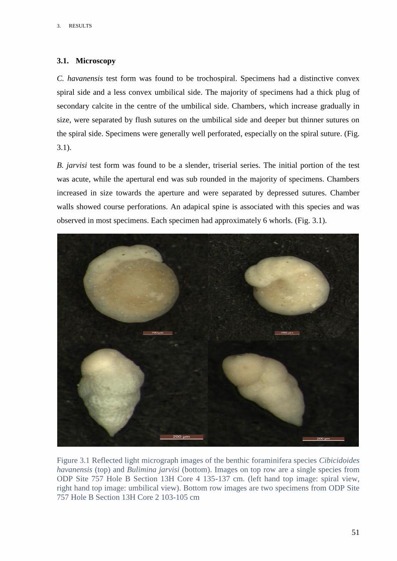
3. RESULTS

51

3.1. Microscopy

C. havanensis test form was found to be trochospiral. Specimens had a distinctive convex

spiral side and a less convex umbilical side. The majority of specimens had a thick plug of

secondary calcite in the centre of the umbilical side. Chambers, which increase gradually in

size, were separated by flush sutures on the umbilical side and deeper but thinner sutures on

the spiral side. Specimens were generally well perforated, especially on the spiral suture. (Fig.

3.1).

B. jarvisi test form was found to be a slender, triserial series. The initial portion of the test

was acute, while the apertural end was sub rounded in the majority of specimens. Chambers

increased in size towards the aperture and were separated by depressed sutures. Chamber

walls showed course perforations. An adapical spine is associated with this species and was

observed in most specimens. Each specimen had approximately 6 whorls. (Fig. 3.1).

Figure 3.1 Reflected light micrograph images of the benthic foraminifera species Cibicidoides

havanensis (top) and Bulimina jarvisi (bottom). Images on top row are a single species from

ODP Site 757 Hole B Section 13H Core 4 135-137 cm. (left hand top image: spiral view,

right hand top image: umbilical view). Bottom row images are two specimens from ODP Site

757 Hole B Section 13H Core 2 103-105 cm

3. RESULTS

52

3.2. Foraminiferal Average Test Masses

The epifaunal foraminiferal test mass, recovered from C. havanensis, showed variation

between 30 and 37 million years before present. The dataset included 62 samples and returned

a mean mass of 84.85 µg (Fig. 3.2a). Mass values ranged from 49.83 to 144.83 µg. The mean

mass of epifaunal tests before the initiation of the EOT was 63.49 µg, while during the EOT

the epifaunal test mass rose to 88.64 µg. After the EOT, the mean epifaunal test mass

increased further to 102.23 µg. Post EOT, epifaunal test mass was significantly higher

compared to pre EOT concentrations. The relative standard deviation (RSD) before the EOT

was 16% (n=25) while after the EOT RSD fell to 15% (n=29). During the EOT the RSD of

the data was significantly higher at 27% (n=8).

The infaunal foraminiferal test mass, recovered from B. jarvisi, showed some variation


a mean mass of 34.54 µg (Fig. 3.2b). Values ranged from 26 to 41.57 µg. The mean mass of

infaunal tests before the initiation of the EOT was 32.57 µg, while during the EOT the mean

infaunal test mass dropped to 31.65 µg. After the EOT, the mean infaunal test mass increased

to 36.95 µg. Post EOT, mean infaunal test mass was higher compared to pre EOT

concentrations. The relative standard deviation (RSD) before the EOT was 10% (n=25) while

after the EOT RSD had fallen to 6% (n=27). During the EOT the RSD was 8% (n=7).

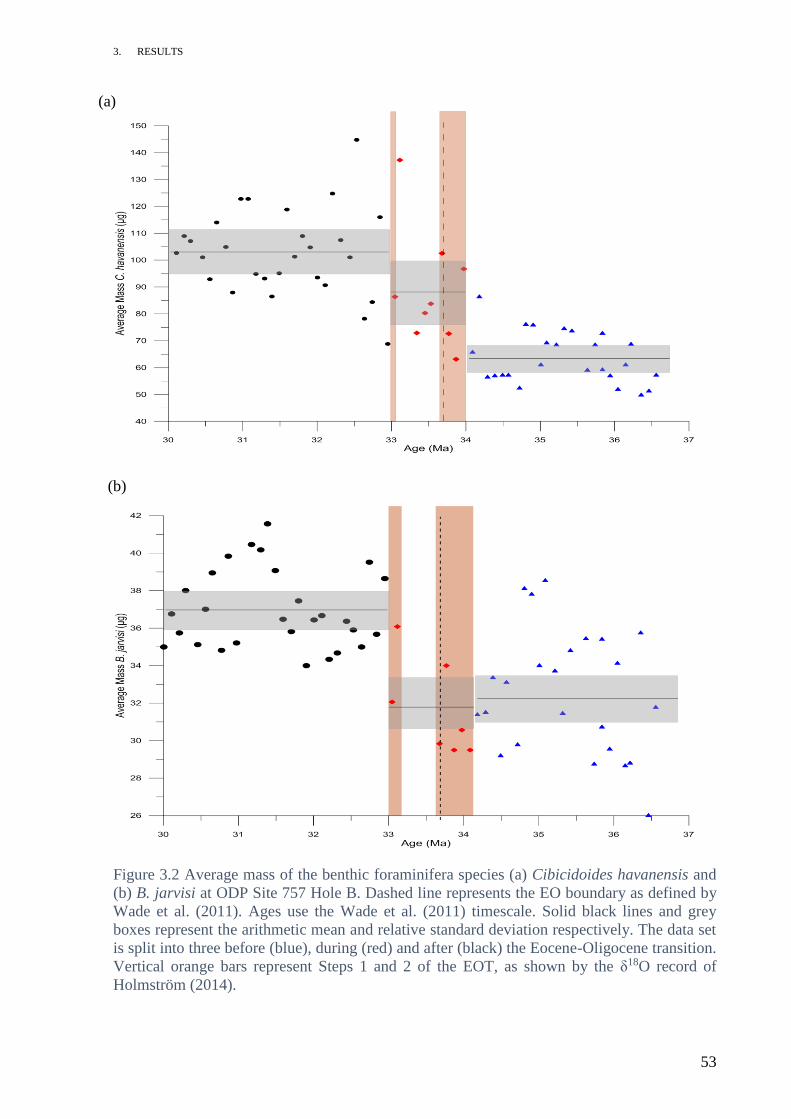
3. RESULTS

53

Figure 3.2 Average mass of the benthic foraminifera species (a) Cibicidoides havanensis and

(b) B. jarvisi at ODP Site 757 Hole B. Dashed line represents the EO boundary as defined by

Wade et al. (2011). Ages use the Wade et al. (2011) timescale. Solid black lines and grey

boxes represent the arithmetic mean and relative standard deviation respectively. The data set

is split into three before (blue), during (red) and after (black) the Eocene-Oligocene transition.

Vertical orange bars represent Steps 1 and 2 of the EOT, as shown by the δ18O record of

Holmström (2014).

(a)

(b)

3. RESULTS

54

3.3. Species Abundances

The abundance of C. havanensis showed variation between 30 and 37 million years before

present. The dataset included 63 samples and returned a mean abundance of 12.73 specimens

per gram of coarse fraction (Fig. 3.3). Abundance values ranged from 1.02 to 53.85 specimens

per gram of coarse fraction. The mean abundance of C. havanensis before the initiation of the

EOT was 16.28 specimens per gram, while during the EOT the mean abundance of C.

havanensis fell to 14.64. After the EOT, the mean abundance of C. havanensis decreased

further to 9.25 specimens per gram. Post EOT, abundance of C. havanensis was significantly

lower compared to pre EOT concentrations. During Step 1, abundance of C. havanensis

dropped by 13.63 specimens per gram, while during Step 2 C. havanensis abundance

increased by 5.42 specimens per gram.

The abundance of B. jarvisi showed variation between 30 and 37 million years before present.

The dataset included 59 samples and returned a mean abundance of 18.55 specimens per gram

of coarse fraction (Fig. 3.3). Abundance values ranged from 4.08 to 53.85 specimens per gram

coarse fraction. The mean abundance of B. jarvisi before the initiation of the EOT was 22.64

specimens per gram, while during the EOT the mean abundance of B. jarvisi rose to 22.81.

After the EOT, the mean abundance of B. jarvisi decreased to 14.29 specimens per gram. Post

EOT, abundance of B. jarvisi was significantly lower compared to pre EOT concentrations.

During Step 1 abundance of B. jarvisi drops by 34 specimens per gram, while during Step 2

B. jarvisi abundance increases by 5.17 specimens per gram.

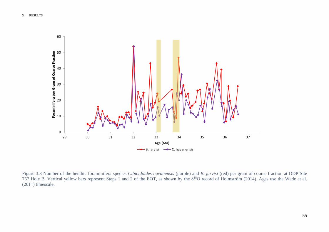
3. RESULTS

55

Figure 3.3 Number of the benthic foraminifera species Cibicidoides havanensis (purple) and B. jarvisi (red) per gram of course fraction at ODP Site

757 Hole B. Vertical yellow bars represent Steps 1 and 2 of the EOT, as shown by the δ18O record of Holmström (2014). Ages use the Wade et al.

(2011) timescale.

0

10

20

30

40

50

60

29 30 31 32 33 34 35 36 37

Fora

min

ife

ra p

er

Gra

m o

f C

oar

se F

ract

ion

Age (Ma)

B. jarvisi C. havanensis

3. RESULTS

56

3.4. Foraminiferal Mg/Ca

The epifaunal magnesium calcium record, recovered from C. havanensis, showed variation


a mean Mg/Ca ratio of 1.1 mmol/mol (Fig. 3.4). Mg/Ca values ranged from 0.92 to 1.29

mmol/mol. The mean value of epifaunal foraminiferal Mg/Ca was 1.07 mmol/mol before the

initiation of the EOT, while during the EOT the mean Mg/Ca concentration rose to 1.1

mmol/mol. After the EOT the mean Mg/Ca remained relatively elevated at 1.13 mmol/mol.

Post EOT Mg/Ca concentrations were slightly raised compared with pre EOT concentrations.

During Step 1 of the EOT epifaunal Mg/Ca increased by 0.14 mmol/mol from 1.14

mmol/mol. While the trend across Step 1 was positive, the data peaked and troughed during

this period. Increases during Step 1 were generally two times the magnitude of decreases.

Across Step 2, an increase of 0.1 mmol/mol Mg/Ca was observed, rising to 1.18 mmol/mol.

In between the two steps, a marked decrease in Mg/Ca occurred falling by 0.08 mmol/mol to

1.08 mmol/mol before rising to 1.17 mmol/mol. This decrease took place directly after 33.7

Ma, the EO boundary. After the EOT, Mg/Ca continued to increase, peaking at 1.29

mmol/mol (32.3 Ma), before decreasing to 0.99 mmol/mol between 32.3 and 31.5 Ma.

The infaunal Mg/Ca record, recovered from B. jarvisi, also showed significant variation


a mean Mg/Ca ratio of 1.78 mmol/mol (Fig. 3.4). Mg/Ca values ranged from 1.5 to 2.13

mmol/mol. The mean value of infaunal foraminiferal Mg/Ca was 1.73 mmol/mol before the

initiation of the EOT, while during the EOT the mean Mg/Ca concentration rose to 1.8

mmol/mol. After the EOT the mean Mg/Ca increased further to 1.85 mmol/mol. Post EOT

Mg/Ca levels were raised compared with pre EOT levels. During Step 1 of the EOT, infaunal

Mg/Ca increased by 0.07 mmol/mol to 1.77 mmol/mol. While the trend across Step 1 was

positive, the data peaked and troughed during this period. Between Steps 1 and 2 Bulimina

jarvisi disappeared from the fossil record and therefore Mg/Ca concentrations were not

recorded. This disappearance takes place directly after 33.7 Ma, the EO boundary. The

species does not reappear until the commencement of Step 2. An increase of 0.12 mmol/mol

occurred between Steps 1 and 2. Across Step 2, infaunal Mg/Ca increased to 2.13 mmol/mol

from 1.89 mmol/mol. After the EOT (from 33 Ma to 30Ma) Mg/Ca decreased steadily

(Range: 2.13 mmol/mol to 1.5 mmol/mol).

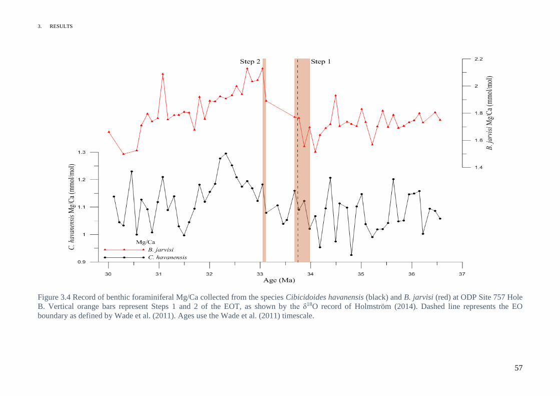
3. RESULTS

57

Figure 3.4 Record of benthic foraminiferal Mg/Ca collected from the species Cibicidoides havanensis (black) and B. jarvisi (red) at ODP Site 757 Hole

B. Vertical orange bars represent Steps 1 and 2 of the EOT, as shown by the δ18O record of Holmström (2014). Dashed line represents the EO

boundary as defined by Wade et al. (2011). Ages use the Wade et al. (2011) timescale.

3. RESULTS

58

3.5. Foraminiferal Li/Ca

The epifaunal lithium calcium record, recovered from C. havanensis, showed variation


a mean Li/Ca ratio of 8.29 mmol/mol (Fig. 3.5). Li/Ca values ranged from 7.4 to 10.1

mmol/mol. The mean value of epifaunal foraminiferal Li/Ca was 8 mmol/mol before the

initiation of the EOT, while during the EOT the mean Li/Ca concentration rose to 8.32

mmol/mol. After the EOT, the mean Li/Ca remained relatively elevated at 8.56 mmol/mol.

Post EOT Li/Ca levels were raised compared with pre EOT levels. During Step 1 of the

Eocene Oligocene transition, epifaunal Li/Ca decreased by 0.12 mmol/mol to 7.6 mmol/mol.

In between the two steps, a marked increase in Li/Ca occurred, rising 1.57 by mmol/mol to

9.16 mmol/mol. This increase took place directly after 33.7 Ma, the EO boundary. Across

Step 2, Li/Ca decreased by 0.24 mmol/mol, however this was followed immediately by an

increase of 0.24 mmol/mol. After the EOT, Li/Ca decreased to 7.98 mmol/mol, a drop of 1.18

mmol/mol (32.3 Ma), before levelling off between 32.3 and 31.07 Ma. A strongly positive

trend in Li/Ca values was observed from 31 Ma onward. Outliers, well outside the general

trend of the data, were observed at 30.1, 30.46 and 36.05 Ma.

The infaunal lithium calcium record, recovered from B. jarvisi, also showed significant

variation between 30 and 37 million years before present. The dataset includes 53 samples

and returned a mean Li/Ca ratio of 7.4 mmol/mol (Fig. 3.5). Li /Ca values ranged from 6.22 to

9.04 mmol/mol. The mean value of infaunal foraminiferal Li/Ca was 6.84 mmol/mol before

the initiation of the EOT, while during the EOT mean Li/Ca concentration rose to 7.36

mmol/mol. After the EOT, the mean Li/Ca increased further to 7.94 mmol/mol. Post EOT,

Li/Ca levels were notably raised compared with pre EOT levels. During Step 1 of the Eocene

Oligocene transition, infaunal Li/Ca increased from 6.75mmol/mol by 0.34 mmol/mol.

Between Steps 1 and 2, Bulimina jarvisi disappeared from the fossil record and therefore

Li/Ca concentration was not recorded. This disappearance took place directly after 33.7 Ma,

the EO boundary. The species does not reappear until the commencement of Step 2. Upon the

re-emergence of the species, Li/Ca concentration was significantly raised by 0.77 mmol/mol.

After the EOT, Li/Ca remains relatively constant with the exception of two peaks at 32 Ma

and 31.7 Ma.

3. RESULTS

59

Figure 3.5 Record of benthic foraminiferal Li/Ca collected from the species Cibicidoides havanensis (black) and B. jarvisi (red) at ODP Site 757 Hole



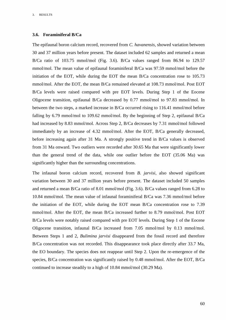
3. RESULTS

60

3.6. Foraminiferal B/Ca

The epifaunal boron calcium record, recovered from C. havanensis, showed variation between

30 and 37 million years before present. The dataset included 62 samples and returned a mean

B/Ca ratio of 103.75 mmol/mol (Fig. 3.6). B/Ca values ranged from 86.94 to 129.57

mmol/mol. The mean value of epifaunal foraminiferal B/Ca was 97.59 mmol/mol before the

initiation of the EOT, while during the EOT the mean B/Ca concentration rose to 105.73

mmol/mol. After the EOT, the mean B/Ca remained elevated at 108.73 mmol/mol. Post EOT

B/Ca levels were raised compared with pre EOT levels. During Step 1 of the Eocene

Oligocene transition, epifaunal B/Ca decreased by 0.77 mmol/mol to 97.83 mmol/mol. In

between the two steps, a marked increase in B/Ca occurred rising to 116.41 mmol/mol before

falling by 6.79 mmol/mol to 109.62 mmol/mol. By the beginning of Step 2, epifaunal B/Ca

had increased by 8.83 mmol/mol. Across Step 2, B/Ca decreases by 7.31 mmol/mol followed

immediately by an increase of 4.32 mmol/mol. After the EOT, B/Ca generally decreased,

before increasing again after 31 Ma. A strongly positive trend in B/Ca values is observed

from 31 Ma onward. Two outliers were recorded after 30.65 Ma that were significantly lower

than the general trend of the data, while one outlier before the EOT (35.06 Ma) was

significantly higher than the surrounding concentrations.

The infaunal boron calcium record, recovered from B. jarvisi, also showed significant

variation between 30 and 37 million years before present. The dataset included 50 samples

and returned a mean B/Ca ratio of 8.01 mmol/mol (Fig. 3.6). B/Ca values ranged from 6.28 to

10.84 mmol/mol. The mean value of infaunal foraminiferal B/Ca was 7.36 mmol/mol before

the initiation of the EOT, while during the EOT mean B/Ca concentration rose to 7.39

mmol/mol. After the EOT, the mean B/Ca increased further to 8.79 mmol/mol. Post EOT

B/Ca levels were notably raised compared with pre EOT levels. During Step 1 of the Eocene

Oligocene transition, infaunal B/Ca increased from 7.05 mmol/mol by 0.13 mmol/mol.

Between Steps 1 and 2, Bulimina jarvisi disappeared from the fossil record and therefore

B/Ca concentration was not recorded. This disappearance took place directly after 33.7 Ma,

the EO boundary. The species does not reappear until Step 2. Upon the re-emergence of the

species, B/Ca concentration was significantly raised by 0.48 mmol/mol. After the EOT, B/Ca

continued to increase steadily to a high of 10.84 mmol/mol (30.29 Ma).

3. RESULTS

61

Figure 3.6 Record of benthic foraminiferal B/Ca collected from the species Cibicidoides havanensis (black) and B. jarvisi (red) at ODP Site 757 Hole



3. RESULTS

62

3.7. Foraminiferal Sr/Ca

The epifaunal strontium calcium record, recovered from C. havanensis, showed some

variation between 30 and 37 million years before present. The dataset included 62 samples

and returned a mean Sr/Ca ratio of 0.85 mmol/mol (Fig.3.7). Sr/Ca values ranged from 0.76 to

0.94 mmol/mol. The mean value of epifaunal foraminiferal Sr/Ca was 0.85 mmol/mol before

the initiation of the EOT, while during the EOT the mean Sr/Ca concentration rose to 0.87

mmol/mol. After the EOT, the mean Sr/Ca decreased to 0.86 mmol/mol. Post EOT, Sr/Ca

concentrations were similar to pre EOT concentrations. During Step 1 of the Eocene

Oligocene transition, epifaunal Sr/Ca decreased from 0.87 mmol/mol by 0.08 mmol/mol. In

between the two steps, a marked increase in Sr/Ca occurred between 33.7 and 33.5 Ma rising

by 0.13 mmol/mol to 0.92 mmol/mol before falling by 0.02 mmol/mol. By the beginning of

Step 2, epifaunal Sr/Ca had increased to 0.94 mmol/mol. Across Step 2, Sr/Ca decreases by

0.06 mmol/mol. After the EOT, Sr/Ca remained generally stable at pre EOT concentrations.

An outlier was recorded at 30.06 Ma that was significantly lower than the general trend of the

data.

The infaunal strontium calcium record, recovered from B. jarvisi, also showed some variation


a mean Sr/Ca ratio of 0.52 mmol/mol (Fig. 3.7). Sr/Ca values ranged from 0.45 to 0.62

mmol/mol. The mean value of infaunal foraminiferal Sr/Ca was 0.5 mmol/mol before the

initiation of the EOT, while during the EOT mean Sr/Ca concentration rose to 0.51

mmol/mol. After the EOT, the mean Sr/Ca increased further to 0.54 mmol/mol. Post EOT

Sr/Ca levels were slightly raised compared with pre EOT levels. During Step 1 of the Eocene

Oligocene transition, infaunal Sr/Ca decreased by 0.07 mmol/mol to 0.46 mmol/mol. The

negative trend began at 33.8 Ma, slightly after the commencement of Step 1. In between

Steps 1 and 2, Bulimina jarvisi disappeared from the fossil record and therefore Sr/Ca

concentration was not recorded. This disappearance took place directly after 33.7 Ma, the EO

boundary. The species does not reappear until the commencement of Step 2. Upon the re-

emergence of the species, Sr/Ca concentration was raised by 0.06 mmol/mol. After the EOT,

Sr/Ca concentration remained relatively constant, with a large peak between 30 and 31 Ma.

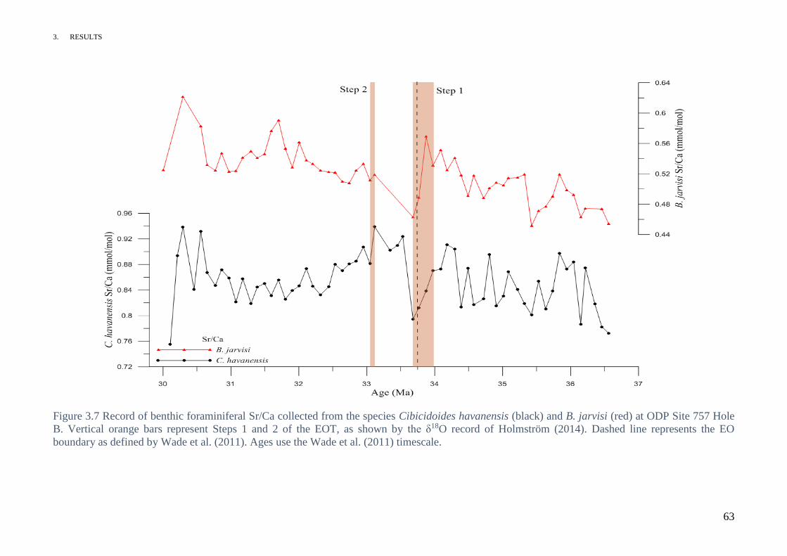
3. RESULTS

63

Figure 3.7 Record of benthic foraminiferal Sr/Ca collected from the species Cibicidoides havanensis (black) and B. jarvisi (red) at ODP Site 757 Hole



3. RESULTS

64

3.8. Foraminiferal U/Ca

The epifaunal uranium calcium record, recovered from C. havanensis, showed variation


a mean U/Ca ratio of 4.3 mmol/mol (Fig. 3.8). U/Ca values ranged from 2.63 to 7.73

mmol/mol. The mean value of epifaunal foraminiferal U/Ca was 3.4 mmol/mol before the

initiation of the EOT, while during the EOT the mean U/Ca concentration rose to 3.77

mmol/mol. After the EOT, the mean U/Ca increased to 5.24 mmol/mol. Post EOT U/Ca

concentrations were higher compared to pre EOT concentrations. During Step 1 of the Eocene

Oligocene transition, epifaunal U/Ca increased from 2.95 mmol/mol to 3.52 mmol/mol, a rise

of 0.57 mmol/mol. In between the two steps, an increase in U/Ca concentration, from 3.52

mmol/mol to 4.43 mmol/mol, occurred. Across Step 2, U/Ca increased by 0.66 mmol/mol

rising to 4.69 mmol/mol. Pre EOT concentrations of U/Ca were stable. After the EOT, U/Ca

continued to increase with a positive trend. By 30.21 Ma, epifaunal U/Ca concentration had

risen as high as 7.73 mmol/mol. An outlier was recorded at 30.06 Ma that was significantly

lower than the general trend of the data.

The infaunal uranium calcium record, recovered from B. jarvisi, also showed variation


a mean U/Ca ratio of 4.54 mmol/mol (Fig 3.8). U/Ca values ranged from 3.17 to 6.15

mmol/mol. The mean value of infaunal foraminiferal U/Ca was 4.06 mmol/mol before the

initiation of the EOT, while during the EOT mean U/Ca concentration rose to 4.45 mmol/mol.

After the EOT, the mean U/Ca increased further to 5.01 mmol/mol. Post EOT, U/Ca levels

were raised compared with pre EOT levels. Upon commencement of Step 1 of the Eocene

Oligocene transition, infaunal U/Ca decreased by 1.11 mmol/mol to 3.47 mmol/mol before

rising by 1.06 mmol/mol. In between Steps 1 and 2, Bulimina jarvisi disappeared from the

fossil record and therefore U/Ca concentration was not recorded. This disappearance took

place directly after 33.7 Ma, the EO boundary. The species does not reappear until the

initiation of Step 2. Upon the re-emergence of the species, U/Ca concentration was raised by

0.63 mmol/mol. After the EOT, U/Ca concentrations were stable until 31.7 Ma. At this point,

U/Ca shifted upward by 1.65 mmol/mol before decreasing slightly to 5.42 mmol/mol. The

infaunal U/Ca signal remains stable from this point Ma forward.

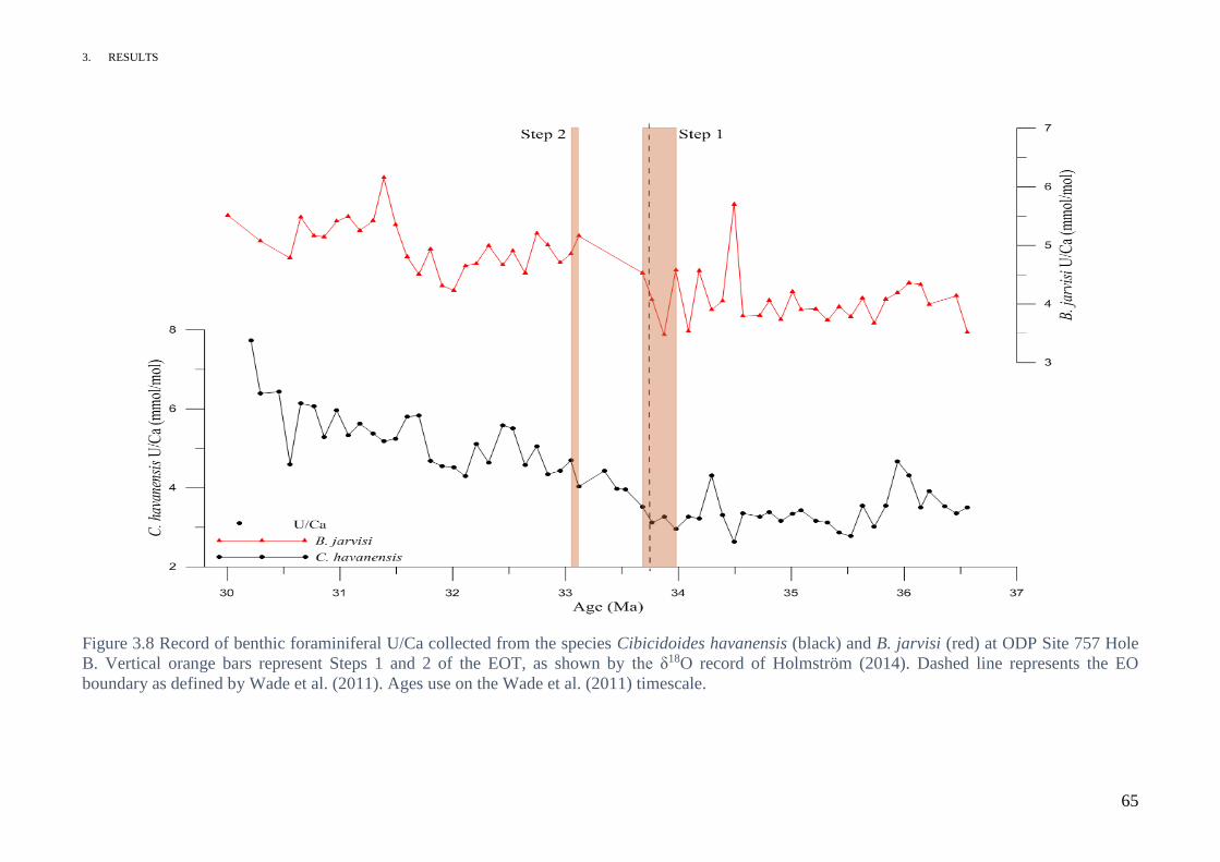
3. RESULTS

65

Figure 3.8 Record of benthic foraminiferal U/Ca collected from the species Cibicidoides havanensis (black) and B. jarvisi (red) at ODP Site 757 Hole


boundary as defined by Wade et al. (2011). Ages use on the Wade et al. (2011) timescale.

4. DISCUSSION

66

4. DISCUSSION

Across the EOT at ODP site 757:

Bottom water temperature change

Saturation state change

Ice volume and sea level changes

Unravelling the foraminiferal Li/Ca, Sr/Ca and U/Ca records

Productivity changes

4. DISCUSSION

*Bottom water temperatures were calculated from Krithe Mg/Ca using the calibration of

Dwyer et al. (2002).

67

4.1. Bottom Water Temperature and Saturation State History at ODP Site 757

4.1.1. Bottom Water Temperature Calculated Using Mg/Ca of B. jarvisi

Bottom water temperature was calculated from B. jarvisi Mg/Ca without correction for

∆[CO32-] because it was assumed that B. jarvisi Mg/Ca was buffered against ∆[CO3

2-]

(Elderfield et al., 2010). This produced a temperature change of +0.87 ⁰C between the

beginning and the end of the EOT (Fig. 4.1). At Tanzanian Drilling Project (TDP) Sites 12

and 17, a -1.2 ⁰C change was calibrated for the same period (Fig. 4.1) (Lear et al., 2008).

Across Step 1, which has been strongly linked with a cooling event, the B. jarvisi bottom

water temperatures marginally increased by 0.16 ⁰C. This is in stark contrast with the -2.8 ⁰C

formulated for Step 1 at TDP Sites 12 and 17 (Lear et al., 2008). Dissolution has been shown

to preferentially remove magnesium rich calcite (Brown and Elderfield, 1996). Therefore, it is

possible that some of apparent warming across Step 1 could be attributed to reduced

dissolution rather than temperature change. Step 2 bottom water temperatures from ODP Site

757 are somewhat easier to correlate with the TDP sites than those for Step 1. From the

beginning to the end of Step 2, a +0.45 ⁰C was formulated for ODP Site 757, a change

comparable to the ~0.5 ⁰C calculated by Lear et al. (2008) for TDP Sites 12 and 17.

The pilot investigation conducted by the author for this study, found that Mg/Ca bottom water

temperatures, formulated using the ostracod genus Krithe*, changed by -0.13 ⁰C at Step 1 and

+0.68 ⁰C at Step 2 (Fig. 4.1). Again the temperature change at Step 2 appears to be

comparable with published records, however the decrease at Step 1 is approximately three

times smaller than the one presented in Lear et al. (2008). As with infaunal foraminifera, such

as B. jarvisi, ostracods have been predicted to be relatively buffered against saturation state

change (Dwyer et al., 2002).

If these species’ Mg/Ca concentrations were buffered against saturation state change, the

temperatures produced would correlate with the TDP sites, which were very well preserved

and located well above the CCD. Across Step 1, a significant cooling is expected, due to the

magnitude of the upward shift in foraminiferal δ18O and the lack of ice growth stimulus (Lear

et al., 2008). Some cooling is required to explain the size of the shift in foraminiferal δ18O

across Step 2. The size and/or lack of cooling predicted by these Mg/Ca paleotemperatures

across Steps 1 and 2 is incompatible with other geochemical proxy information published for

4. DISCUSSION

68

the EOT. It is suggested here that, contrary to Elderfield et al. (2010) and Dwyer et al. (1995)

respectively, both B. jarvisi and Krithe spp. Mg/Ca are affected by changes in saturation state.

A reliable way of quantifying changes in saturation state has not been published for either of

these species. Therefore, their use as indicators of past climate is restricted to sites well above

the calcite compensation depth or periods for which carbonate chemistry in the ocean

remained the same.

4. DISCUSSION

69

Figure 4.1 Record of change in bottom water temperature at ODP Site 757B relative to the

oldest sample, for the benthic foraminifera B. jarvisi (red) and the ostracod species Krithe spp.

(blue). Ages use on the Wade et al. (2011) timescale. Vertical orange bars represent Steps 1

and 2 of the EOT, as shown by the δ18O record of Holmström (2014). Dashed line represents

the EO boundary as defined by Wade et al. (2011). Black line shows the absolute bottom

water temperatures calculated for TDP Sites 12 and 17 from Cibicidoides spp. (Lear et al.,

2008) plotted against the timescale of Cande and Kent (1995). Vertical green bars represent

Step 1 and 2 of the EOT, as shown by the δ18O record of Coxall et al. (2005).

Age (Ma), Cande and Kent (1995) time scale

C

ha

nge

in

Bo

tto

m W

ate

r T

em

pe

ratu

re (

⁰C)

4. DISCUSSION

70

4.1.2. Saturation State Change Calculated Using B/Ca of C. havanensis

As the use of B. jarvisi Mg/Ca to calculate paleotemperatures was unsuccessful, it became the

necessary to calculate saturation state change in order to separate the temperature signal from

the signal caused by saturation state change. Through the use of C. havanensis B/Ca,

saturation state change was quantified. Across the EOT, a clear increase in saturation state

occurred, rising by 18.17 µmol kg-1 (Fig.4.2). This is to be expected when considering the ~1

km deepening of the CCD across the same period. The decrease of 23.88 µmol kg-1 that starts

at 34.18 Ma, marginally before the initiation of Step 1, and lasts 400 Ka is less expected. A

dissolution hypothesis explaining why temperatures appear to warm across Step 1 can be

discounted because saturation state decreased. This would have coincided with increased

dissolution across Step 1. The large increase of 29.88 µmol kg-1 between Step 1 and 2

suggests a significant change in carbonate chemistry within the ocean. It seems plausible that

this increase was caused by the predicted deepening of the CCD. Across Step 2, a small

decrease of 4.33 µmol kg-1 was calculated.

The effect of saturation state change on foraminiferal Mg/Ca was quantified using the B/Ca

derived Δ[CO32−]. The relationship of 0.0086 mmol mol-1 Mg/Ca per µmol kg-1 change in

Δ[CO32−] was used (Elderfield et al., 2006). A rise of 0.16 mmol mol-1 Mg/Ca across the EOT

was found, while the ~29 µmol kg-1 increase in saturation state that occurred just before Step

2 caused foraminiferal Mg/Ca to rise by 0.25 mmol mol-1. The decrease ending midway

through Step 1 shifted Mg/Ca concentrations down by 0.21 mmol mol-1.

The implications to Mg/Ca paleotemperatures of these findings are varied. Temperature

change calculated for Step 1 is likely to be higher than the true change, while the same is true

for Step 2. Any temperature change calculated using Mg/Ca records for between Step 1 and 2

will be notably lower than the true change in temperature.

4. DISCUSSION

71

Figure 4.2 Record of saturation state change relative to the oldest sample at ODP Site 757

Hole B, as calculated from the B/Ca of Cibicidoides havanensis (black: red triangles). Change

in foraminiferal δ18O across the Eocene-Oligocene transition at ODP Site 757B (black: black

diamonds) (Holmström, 2014). Vertical orange bars represent Steps 1 and 2 of the EOT, as

shown by the δ18O record of Holmström (2014). Ages use the Wade et al. (2011) timescale.

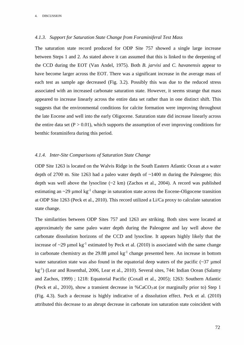
4. DISCUSSION

72

4.1.3. Support for Saturation State Change from Foraminiferal Test Mass

The saturation state record produced for ODP Site 757 showed a single large increase

between Steps 1 and 2. As stated above it can assumed that this is linked to the deepening of

the CCD during the EOT (Van Andel, 1975). Both B. jarvisi and C. havanensis appear to

have become larger across the EOT. There was a significant increase in the average mass of

each test as sample age decreased (Fig. 3.2). Possibly this was due to the reduced stress

associated with an increased carbonate saturation state. However, it seems strange that mass

appeared to increase linearly across the entire data set rather than in one distinct shift. This

suggests that the environmental conditions for calcite formation were improving throughout

the late Eocene and well into the early Oligocene. Saturation state did increase linearly across

the entire data set (P > 0.01), which supports the assumption of ever improving conditions for

benthic foraminifera during this period.

4.1.4. Inter-Site Comparisons of Saturation State Change

ODP Site 1263 is located on the Walvis Ridge in the South Eastern Atlantic Ocean at a water

depth of 2700 m. Site 1263 had a paleo water depth of ~1400 m during the Paleogene; this

depth was well above the lysocline (~2 km) (Zachos et al., 2004). A record was published

estimating an ~29 µmol kg-1 change in saturation state across the Eocene-Oligocene transition

at ODP Site 1263 (Peck et al., 2010). This record utilized a Li/Ca proxy to calculate saturation

state change.

The similarities between ODP Sites 757 and 1263 are striking. Both sites were located at

approximately the same paleo water depth during the Paleogene and lay well above the

carbonate dissolution horizons of the CCD and lysocline. It appears highly likely that the

increase of ~29 µmol kg-1 estimated by Peck et al. (2010) is associated with the same change

in carbonate chemistry as the 29.88 µmol kg-1 change presented here. An increase in bottom

water saturation state was also found in the equatorial deep waters of the pacific (~37 µmol

kg-1) (Lear and Rosenthal, 2006, Lear et al., 2010). Several sites, 744: Indian Ocean (Salamy

and Zachos, 1999) ; 1218: Equatorial Pacific (Coxall et al., 2005); 1263: Southern Atlantic

(Peck et al., 2010), show a transient decrease in %CaCO3 at (or marginally prior to) Step 1

(Fig. 4.3). Such a decrease is highly indicative of a dissolution effect. Peck et al. (2010)

attributed this decrease to an abrupt decrease in carbonate ion saturation state coincident with

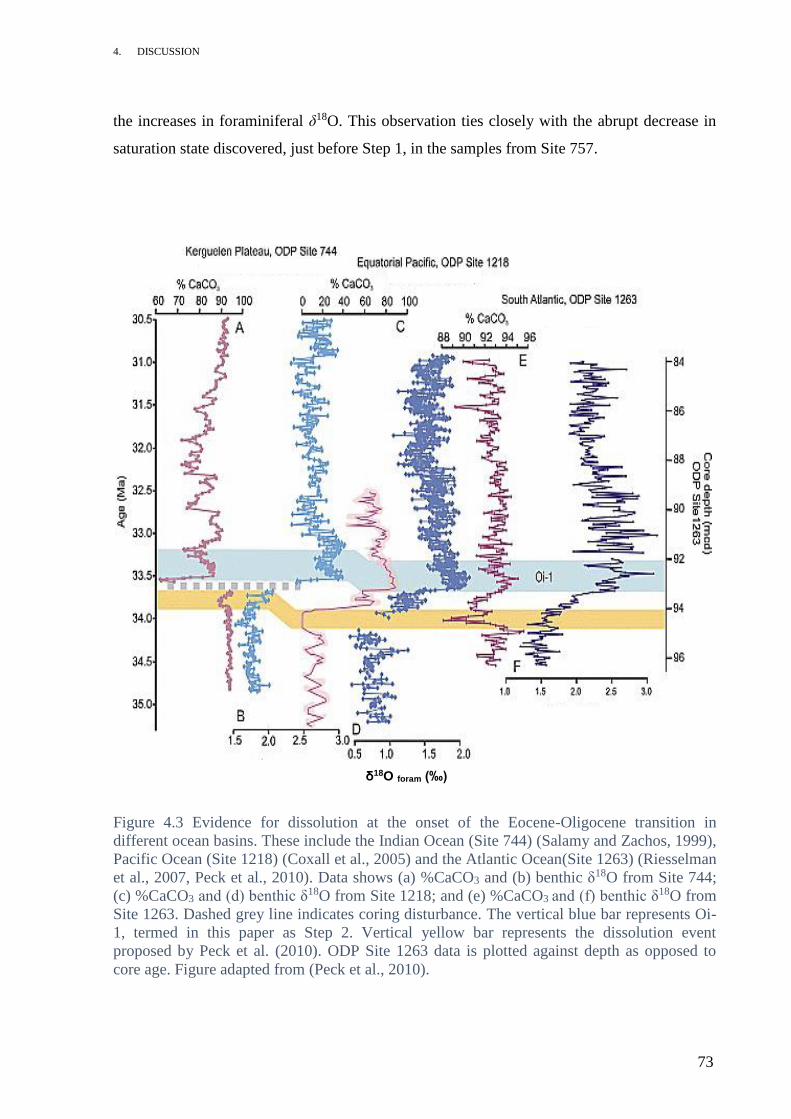
4. DISCUSSION

73

the increases in foraminiferal δ18O. This observation ties closely with the abrupt decrease in

saturation state discovered, just before Step 1, in the samples from Site 757.

Figure 4.3 Evidence for dissolution at the onset of the Eocene-Oligocene transition in

different ocean basins. These include the Indian Ocean (Site 744) (Salamy and Zachos, 1999),

Pacific Ocean (Site 1218) (Coxall et al., 2005) and the Atlantic Ocean(Site 1263) (Riesselman

et al., 2007, Peck et al., 2010). Data shows (a) %CaCO3 and (b) benthic δ18O from Site 744;

(c) %CaCO3 and (d) benthic δ18O from Site 1218; and (e) %CaCO3 and (f) benthic δ18O from

Site 1263. Dashed grey line indicates coring disturbance. The vertical blue bar represents Oi-

1, termed in this paper as Step 2. Vertical yellow bar represents the dissolution event

proposed by Peck et al. (2010). ODP Site 1263 data is plotted against depth as opposed to

core age. Figure adapted from (Peck et al., 2010).

δ18O foram (‰)

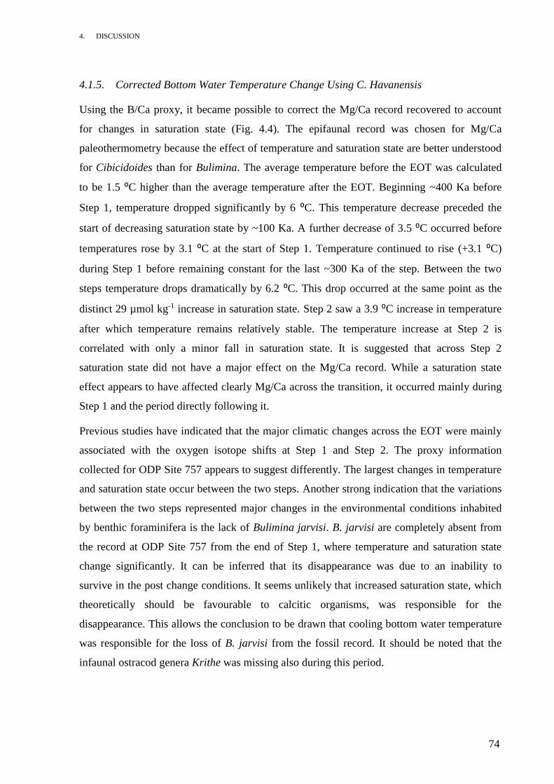
4. DISCUSSION

74

4.1.5. Corrected Bottom Water Temperature Change Using C. Havanensis

Using the B/Ca proxy, it became possible to correct the Mg/Ca record recovered to account

for changes in saturation state (Fig. 4.4). The epifaunal record was chosen for Mg/Ca

paleothermometry because the effect of temperature and saturation state are better understood

for Cibicidoides than for Bulimina. The average temperature before the EOT was calculated

to be 1.5 ⁰C higher than the average temperature after the EOT. Beginning ~400 Ka before

Step 1, temperature dropped significantly by 6 ⁰C. This temperature decrease preceded the

start of decreasing saturation state by ~100 Ka. A further decrease of 3.5 ⁰C occurred before

temperatures rose by 3.1 ⁰C at the start of Step 1. Temperature continued to rise (+3.1 ⁰C)

during Step 1 before remaining constant for the last ~300 Ka of the step. Between the two

steps temperature drops dramatically by 6.2 ⁰C. This drop occurred at the same point as the

distinct 29 µmol kg-1 increase in saturation state. Step 2 saw a 3.9 ⁰C increase in temperature

after which temperature remains relatively stable. The temperature increase at Step 2 is

correlated with only a minor fall in saturation state. It is suggested that across Step 2

saturation state did not have a major effect on the Mg/Ca record. While a saturation state

effect appears to have affected clearly Mg/Ca across the transition, it occurred mainly during

Step 1 and the period directly following it.

Previous studies have indicated that the major climatic changes across the EOT were mainly

associated with the oxygen isotope shifts at Step 1 and Step 2. The proxy information

collected for ODP Site 757 appears to suggest differently. The largest changes in temperature

and saturation state occur between the two steps. Another strong indication that the variations

between the two steps represented major changes in the environmental conditions inhabited

by benthic foraminifera is the lack of Bulimina jarvisi. B. jarvisi are completely absent from

the record at ODP Site 757 from the end of Step 1, where temperature and saturation state

change significantly. It can be inferred that its disappearance was due to an inability to

survive in the post change conditions. It seems unlikely that increased saturation state, which

theoretically should be favourable to calcitic organisms, was responsible for the

disappearance. This allows the conclusion to be drawn that cooling bottom water temperature

was responsible for the loss of B. jarvisi from the fossil record. It should be noted that the

infaunal ostracod genera Krithe was missing also during this period.

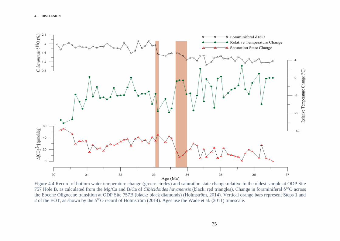
4. DISCUSSION

75

Figure 4.4 Record of bottom water temperature change (green: circles) and saturation state change relative to the oldest sample at ODP Site

757 Hole B, as calculated from the Mg/Ca and B/Ca of Cibicidoides havanensis (black: red triangles). Change in foraminiferal δ18O across

the Eocene Oligocene transition at ODP Site 757B (black: black diamonds) (Holmström, 2014). Vertical orange bars represent Steps 1 and

2 of the EOT, as shown by the δ18O record of Holmström (2014). Ages use the Wade et al. (2011) timescale.

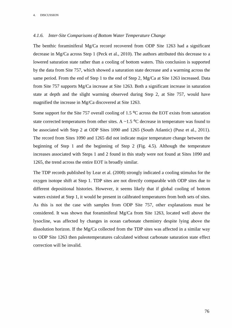
4. DISCUSSION

76

4.1.6. Inter-Site Comparisons of Bottom Water Temperature Change

The benthic foraminiferal Mg/Ca record recovered from ODP Site 1263 had a significant

decrease in Mg/Ca across Step 1 (Peck et al., 2010). The authors attributed this decrease to a

lowered saturation state rather than a cooling of bottom waters. This conclusion is supported

by the data from Site 757, which showed a saturation state decrease and a warming across the

same period. From the end of Step 1 to the end of Step 2, Mg/Ca at Site 1263 increased. Data

from Site 757 supports Mg/Ca increase at Site 1263. Both a significant increase in saturation

state at depth and the slight warming observed during Step 2, at Site 757, would have

magnified the increase in Mg/Ca discovered at Site 1263.

Some support for the Site 757 overall cooling of 1.5 ⁰C across the EOT exists from saturation

state corrected temperatures from other sites. A ~1.5 ⁰C decrease in temperature was found to

be associated with Step 2 at ODP Sites 1090 and 1265 (South Atlantic) (Pusz et al., 2011).

The record from Sites 1090 and 1265 did not indicate major temperature change between the

beginning of Step 1 and the beginning of Step 2 (Fig. 4.5). Although the temperature

increases associated with Steps 1 and 2 found in this study were not found at Sites 1090 and

1265, the trend across the entire EOT is broadly similar.

The TDP records published by Lear et al. (2008) strongly indicated a cooling stimulus for the

oxygen isotope shift at Step 1. TDP sites are not directly comparable with ODP sites due to

different depositional histories. However, it seems likely that if global cooling of bottom

waters existed at Step 1, it would be present in calibrated temperatures from both sets of sites.

As this is not the case with samples from ODP Site 757, other explanations must be

considered. It was shown that foraminiferal Mg/Ca from Site 1263, located well above the

lysocline, was affected by changes in ocean carbonate chemistry despite lying above the

dissolution horizon. If the Mg/Ca collected from the TDP sites was affected in a similar way

to ODP Site 1263 then paleotemperatures calculated without carbonate saturation state effect

correction will be invalid.

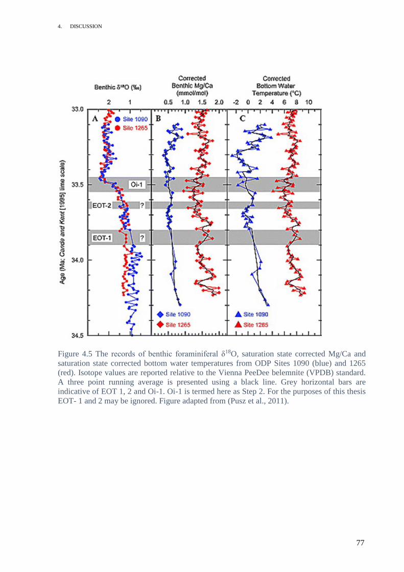
4. DISCUSSION

77

Figure 4.5 The records of benthic foraminiferal δ18O, saturation state corrected Mg/Ca and

saturation state corrected bottom water temperatures from ODP Sites 1090 (blue) and 1265

(red). Isotope values are reported relative to the Vienna PeeDee belemnite (VPDB) standard.

A three point running average is presented using a black line. Grey horizontal bars are

indicative of EOT 1, 2 and Oi-1. Oi-1 is termed here as Step 2. For the purposes of this thesis

EOT- 1 and 2 may be ignored. Figure adapted from (Pusz et al., 2011).

4. DISCUSSION

78

4.1.7. Changes in Ice Volume across the EOT

By applying the Mg/Ca bottom water temperatures, corrected for ∆[CO32−], to the

paleotemperature equation of Shackleton (1974), it was possible to partition the foraminiferal

δ18O into the temperature and δ18Osw components. An approximation of δ18Osw at ODP Site

757 allowed ice volume and sea level change to be calculated (Fig. 4.6).

The average value of δ18Osw before the EOT was found to be 0.2 ‰ lower than after the

transition. Directly before the EOT it was found that δ18Osw decreased markedly. This was

followed by an increase in δ18Osw (0.9 ‰) during the first half of Step 1. At the end of Step 1

δ18Osw drops dramatically by 1.8 ‰. Across Step 2, δ18Osw increased by 1.39 ‰. The oxygen

isotopic ratio within seawater is generally considered to reflect ice volume change. Increases

in global ice volume lower sea level.

For the Pleistocene it was found that a 0.1 ‰ increase in δ18Osw was approximately equal to a

10 m decrease in sea level (Shackleton and Opdyke, 1973). This relationship can be used to

estimate sea level change for other periods where δ18Osw is known. Using the average value of

δ18Osw before and after the EOT, the decrease in sea level across the Eocene-Oligocene

transition would appear to be ~20 m. The increase in δ18Osw during Step 1 represents a 90 m

fall in sea level, while the increase during Step 2 indicates a fall of ~140 m. Between the two

steps, a sea level increase appears to be indicated by the record, rising approximately 180 m.

This large increase corresponds with dramatic falls in temperatures and rises in saturation

state. Cumulatively the changes above indicate a sea level fall of ~50 m during the EOT.

A number of difficulties exist in interpreting these sea level changes. Firstly, concentrating

on the 140 m decrease in sea level at Step 2, it should be noted that a decrease of this size is

not possible when considering Antarctic ice growth alone. More ice would be required than

can be accommodated onto modern day Antarctica. Others have suggested that simultaneous

bipolar glaciation during the early Oligocene would provide enough ice growth to account for

the changes observed here (Coxall et al., 2005, Tripati et al., 2005). However, Edgar et al.

(2007) stated that no +evidence for extreme bipolar glaciation existed for the main Eocene

calcite compensation shift. Two plausible explanations for the ice growth signal observed at

ODP Site 757 remain. Firstly, it is possible that small northern hemisphere valley glaciers and

ephemeral ice caps existed. Some evidence for valley glaciers such as these has been

presented for Greenland during the Eocene-Oligocene transition (Eldrett et al., 2007). The

4. DISCUSSION

79

other explanation centres on the suggestion that the west Antarctic continent was up to 20%

larger in area during the late Eocene than it is in the modern day (Wilson and Luyendyk,

2009), which would allow for significantly more ice growth. A combination of these two may

be a better reflection of the true nature of EOT ice growth. It is safe to say that while a

significant period of Antarctic ice growth and sea level fall did occur during Step 2, it may not

have been of the magnitude shown here. Another factor other than Antarctic ice growth must

have played a role in moderating seawater oxygen isotopes or sea level.

Much the same can be said for the proposed sea level fall during Step 1 as for Step 2.

Previously published records have hypothesised a cooling driven change in foraminiferal

oxygen isotopes during Step 1 (Lear et al., 2008). However, little evidence for this is shown in

the record from ODP Site 757. Changes at Site 757 appear to be driven by ice growth similar

to like Step 2. The magnitude of the sea level fall, predicted by the Site 757 record for Step 1,

is incompatible with current predictions for the level of ice growth across the step. Therefore,

other controls on δ18Osw must be considered. Within the deep ocean δ18Osw is broadly

conservative, changing only due to changes in temperature and mixing (Ravelo and Hillaire-

Marcel, 2007). It is possible that the opening of oceanic gateways and the establishment of the

Antarctic Circumpolar Current modified deep water circulation during the Eocene-Oligocene

transition. Changes in δ18Osw broadly mirror the trends seen in the foraminiferal carbon

isotope record. Since carbon isotopic ratios are affected by mixing water masses, these

changes may provide an indication of mixing processes.

The δ13C ratios for ODP Site 757 (Fig. 4.6) are broadly similar to those for Sites 1265 and

522, while δ13C is approximately 1 ‰ lower at Sites 1090 and 1218. Pusz et al. (2011)

attributed the higher values of δ13C at Sites 1265 and 522 to differing source regions from

those of Sites 1090 and 1218. Therefore, it can be asserted that Site 757 has the same source

region as Sites 1265 and 522. High δ13C ratios are indicative of nutrient depleted waters,

which are likely to have a northerly origin. Unlike Sites 1265 and 522, foraminiferal δ13C is

raised after the EOT. This suggests a more northerly nutrient depleted source region after the

EOT than before it.

Changes in the δ18Osw record may reflect the regional salinity of Site 757 during the EOT.

Both ice growth and precipitation change salinity. Any water mass with a modified salinity

will change δ18Osw if it is mixed with the original bottom waters. Considering this, the

4. DISCUSSION

80

increase in δ18Osw shown at the beginning of Step 1 may indicate a higher regional salinity,

while any decrease in oxygen isotope values could indicate a lower regional salinity. The

increase in δ18Osw during Step 1 could result from the mixing of high salinity waters with

those originally at Site 757. High salinity waters would either indicate ice growth at the

source region or a decrease in precipitation. If the source region for Site 757 bottom had

changed, as could be the case if circulation changed upon the opening of oceanic gateways,

this could result also in modified salinity.

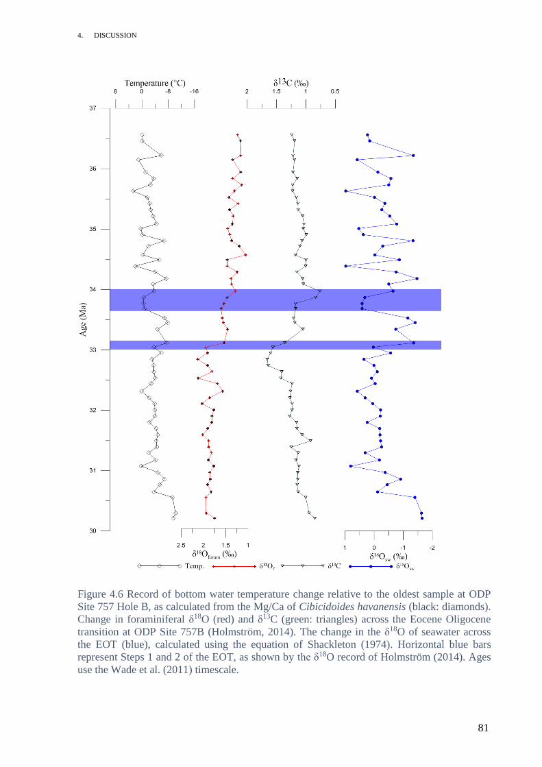
4. DISCUSSION

81

Figure 4.6 Record of bottom water temperature change relative to the oldest sample at ODP

Site 757 Hole B, as calculated from the Mg/Ca of Cibicidoides havanensis (black: diamonds).

Change in foraminiferal δ18O (red) and δ13C (green: triangles) across the Eocene Oligocene

transition at ODP Site 757B (Holmström, 2014). The change in the δ18O of seawater across

the EOT (blue), calculated using the equation of Shackleton (1974). Horizontal blue bars

represent Steps 1 and 2 of the EOT, as shown by the δ18O record of Holmström (2014). Ages

use the Wade et al. (2011) timescale.

4. DISCUSSION

82

4.1.8. Inter-Site Comparisons of δ18Osw

A record of δ18Osw was published for ODP Sites 1090 and 1295 across the EOT (Pusz et al.,

2011). At these sites eustatic sea level fall was shown to be approximately 45-90 m across

Step 2 while no significant ice growth was shown during any other part of the EOT. This ~70

m fall coincident with Step 2 is comparable with the 55-70 m decrease in sea level estimated

for other sites (Pekar et al., 2002, Miller et al., 2008, Katz et al., 2008). It is plausible that the

majority of the Step 2 shift in foraminiferal δ18O is accounted for by the ice volume change

observed at other sites. The studies mentioned above support the assumption of lack of ice

growth during Step 1 (Lear et al., 2008). The records from the above studies differ

significantly from the record recovered from ODP Site 757. Without the cooling associated

with Step 1, it becomes difficult to explain the shift in δ18Osw at Site 757 without large scale

ice growth. The saturation state corrected bottom water temperatures clearly show a

significant warming Over Step 1, in direct conflict with published records. Another problem

is presented by the cooling occurring between the two steps. It seems highly unlikely that ice

volume decreased globally with no indication from any other records. One explanation could

be that the initial prediction of the duration of Step 1 was shorter than the true length. Were

this to be the case, a cooling trend would have occurred across Step 1 going someway to

corroborating evidence from Site 757 with records from other studies. This argument,

however, lacks evidence due to the lack of a rise in foraminiferal δ18O after 33.7 Ma. A higher

resolution isotope record may shed light on this issue.

4. DISCUSSION

83

4.2. Indications from the Foraminiferal Li/Ca, Sr/Ca and U/Ca Records

4.2.1. Li/Ca

The temperature and saturation state changes, formulated using Mg/Ca and B/Ca, are

supported by the lithium calcium record of C. havanensis (Fig. 4.7a). As stated in section

4.1.6., before Step 1, temperature increased and saturation state fell. Over the same period the

Li/Ca signal decreased. Falling foraminiferal Li/Ca ratios are associated with decreasing

carbonate saturation state and increasing temperature. Therefore, the decrease in the Li/Ca

record presented here for Step 1 at Site 757 indicates strongly that the rising temperatures and

falling carbonate saturation state changes calculated from Mg/Ca are valid. The same can be

applied to the changes that occur between the two steps and for Step 2. The large cooling that

took place just after the EO boundary is coupled with a significant increase in saturation state.

As expected Li/Ca concentrations also increased. Changes in foraminiferal Li/Ca across Step

2 were in line with changes to bottom water temperature and saturation state. However, the

magnitude of these changes was negligible with regard to the resolution of the record. The

Li/Ca record consistently supports the calculated bottom water temperature and carbonate

saturation state records. Away from the EOT, the carbonate saturation state increases

significantly around 30 Ma. This is supported by increases in the foraminiferal Li/Ca record.

Therefore, it can be assumed that a significant saturation state increase did occur well after the

EOT, towards the middle Oligocene.

Comparing the foraminiferal Li/Ca collected from Site 757 samples with those collected from

Site 1263 reveals similarities in the trends observed at Step 1 (Fig. 4.7b). Li/Ca from Site

1263 increases by 2 mmol/mol prior to Step 1, before decreasing by 1 mmol/mol during Step

1. The initial rise in Li/Ca coincides with a rise in %CaCO3. Decreases in Li/Ca coincide with

decreasing %CaCO3 during Step 1. The Site 757 Li/Ca values mirror this trend, however

increases and decreases are about half the magnitude of those at Site 1263. This may be

explained by the use of different species or the differing site location. Interestingly, the

decreasing Li/Ca during Step 1 at Site 757 ties closely with the decreasing %CaCO3 shown to

exist at many other sites (Fig. 4.3). This further supports the theory that before the EOT a

large scale dissolution event occurred.

4. DISCUSSION

84

Figure 4.7 (a) Record of bottom water temperature (blue) and saturation state change (black)

relative to the oldest sample at ODP Site 757 Hole B, as calculated from the Mg/Ca and B/Ca

of Cibicidoides havanensis. Change in foraminiferal Li/Ca (red) across the Eocene Oligocene

transition at ODP Site 757B. Horizontal blue bars represent Steps 1 and 2 of the EOT, as

shown by the δ18O record of Holmström (2014). Ages use the Wade et al. (2011) timescale.

(b) a record of %CaCO3 (Riesselman et al., 2007) and benthic foraminiferal Li/Ca (Peck et al.,

2010) from ODP Site 1263. Figure 4.7b adapted from (Peck et al., 2010).

(b)

(a)

4. DISCUSSION

85

4.2.2. Sr/Ca

The foraminiferal Sr/Ca ratios from ODP Site 757 were rising until the beginning of Step 1 of

the EOT before dropping dramatically during Step 1. The concentrations of foraminiferal

Sr/Ca then increase between Steps 1 and 2 by around the same magnitude as the preceding

decrease. These trends are observed in both infaunal and epifaunal records. Compared with

these changes, foraminiferal Sr/Ca after the EOT is relatively stable. This indicates that a

saturation state decrease occurred during Step 1, while an increase in saturation state occurred

between the two steps. The assumption that the increases and decreases observed in

foraminiferal Sr/Ca ratios across the EOT are caused by a saturation state effect are supported

by the saturation state changes calculated from the B/Ca record, as well as the trends observed

within benthic foraminiferal Li/Ca. Foraminiferal Sr/Ca ratios are affected also by changing

water depth (of the order of -0.1 mmol/mol per km depth increase (Lear et al., 2003)).

Therefore, if paleowater depth changed across the EOT at Site 757, it may account for some

of the change observed in foraminiferal Sr/Ca ratios, which previously has been attributed to

saturation state change.

The rapid decreases in foraminiferal Sr/Ca discovered at Sites 1219 and 1220 after the

initiation of Step 2 are not seen in the record from Site 757 (Mawbey, 2012). The Site 757

record more closely resembles the trends observed at Site 1218, however these are not shown

clearly. The foraminiferal Sr/Ca concentrations at Site 1218 are relatively constant before and

after the transition, while between Steps 1 and 2 Sr/Ca decreases and then increases (Mawbey,

2012). These changes are of a similar magnitude. The Site 1218 decrease-increase trend is

remarkably similar to the one presented for ODP Site 757. If not for the significantly different

time span of the increase-decrease and that the two sites Sr/Ca match different parts of the

foraminiferal 18O record, it would be easy to see a clear correlation between the

foraminiferal Sr/Ca of the two sites. Higher resolution oxygen isotope analysis and plotting

both records on the same age model may yet show that these events occurred at the same

time. The radically differing trends shown at different sites of Leg 199 (Sites 1215-1222)

allowed Mawbey (2012) to conclude that changing seawater Sr/Ca was not the causal

mechanism of the decreases. The lack of the rapid decrease in foraminiferal Sr/Ca in the Site

757 record supports this conclusion.

4. DISCUSSION

86

4.2.3. U/Ca

The uranium calcium concentration within various Cibicidoides species (mundulus and

wuellerstorfi) has been shown to increase with decreasing carbonate saturation state (Fig 1.5)

(Raitzsch et al., 2011). With this in mind, both the infaunal record recovered from B. jarvisi

and the epifaunal record recovered from C. havanensis indicate a fall in carbonate saturation

state across the EOT at Site 757. The epifaunal record is relatively stable until the EO

boundary, at 33.7 Ma, at which point it rises steadily until 30 Ma. Due to the disappearance of

B. jarvisi from the fossil record between the two steps of the EOT, the infaunal U/Ca appears

to shift upward dramatically. This shift may be gentler, however this is impossible to prove

due to the lack of data. Whether gentle or steep, the increase in the infaunal U/Ca record

supports the assumption that saturation state decrease occurred across the EOT. The upward

trend in U/Ca concentrations was reproduced at sites on ODP Leg 199 (Mawbey, 2012).

Increasing mass accumulation rate of carbonate, CCD deepening, % calcium carbonate and

better shell preservation were all listed as reasons why increasing U/Ca could not indicate a

saturation state decrease across the EOT (Mawbey, 2012). The data collected from

foraminifera at Site 757 strongly supports the lack of a saturation state decrease across the

EOT. Calculated changes in saturation state show a clear increase between Step 1 and 2 of the

EOT. The increase is supported by the Li/Ca and Sr/Ca ratios. As sites in both the equatorial

Pacific Ocean and the Indian Ocean both show the increasing trend in U/Ca and saturation

state increase, it can be concluded that another mechanism is controlling U/Ca during this

period.

The relationship the U/Ca is negatively correlated with saturation state may not be true for the

species investigated in this study. However, due to the close genetic relationship of C.

havanensis and C. mundulus this can be ruled out. While it is expected that only redox

chemistry of the seafloor and saturation state have an effect on benthic foraminifera, it is

possible that bottom water temperature plays a role. The U/Ca of some planktonic

foraminifera has a temperature component, which results in a positive relationship between

temperature and U/Ca (Yu et al., 2008). Were this the case with the benthic foraminifera

studied at Site 757 and Leg 199, then a warming is indicated by the data. As a warming is not

shown by the Site 757 saturation state corrected bottom waters temperatures, this seems

unlikely. Records of bottom water temperatures from sites unaffected by saturation state

4. DISCUSSION

87

change indicate a cooling across the EOT, further ruling out warming as the causal

mechanism for increasing U/Ca (Lear et al., 2008).

Changes in the oxygen concentrations of pore waters can increase or decrease the levels of

authigenic, uranium bearing material being precipitated. However, no evidence exists for

changing redox conditions at the seafloor during the EOT. Further, the fact that the trend in

U/Ca occurs in two ocean basins seems to suggest that this change in pore water oxygen

concentration would have to be a global event, a highly unlikely scenario. Mawbey (2012)

attributed the increases in U/Ca concentration at leg 199 to a decreasing dissolution effect

across the EOT. It was noted that dissolution preferentially removes high uranium carbonate

from foraminifera (Russell et al., 2004, Yu et al., 2008). Were this the case, as saturation state

increases dissolution would fall in turn increasing U/Ca. This seems a likely explanation for

the trends in foraminiferal U/Ca observed at Site 757. It is suggested here that use of U/Ca as

an indicator of saturation state change is highly limited by the conflicting signal from

dissolution. While work is required to quantify the effect of dissolution on foraminiferal

U/Ca, it may be the case that U/Ca is better suited as a proxy for dissolution than it is for

saturation state.

A dissolution effect, as proposed above, has serious implications on the bottom water

temperatures calculated using Mg/Ca paleothermometry. If Mg/Ca is affected by dissolution

in a similar way to U/Ca, which has previously been proposed by Brown and Elderfield

(1996), some of the increase in foraminiferal Mg/Ca discovered at Site 757 may be due to a

dissolution affect. Mawbey (2012) attributed ~0.4 mmol/mol of the increase in foraminiferal

Mg/Ca at ODP Site 1218 to a dissolution affect such as this. Bar the U/Ca evidence, proof for

a dissolution effect is somewhat lacking. Therefore, more study is required before a definitive

conclusion can be drawn as to whether dissolution affected trace metal ratios in benthic

foraminifera across the EOT.

4. DISCUSSION

88

4.3. Surface Productivity Changes across the EOT

Abundance of benthic foraminifera provides a first order indication of surface productivity.

Here B. jarvisi abundance is discussed because it has been proposed as an excellent indicator

of surface productivity (Thomas et al., 1995). Abundances were clearly variable before the

EOT. These short term fluctuations occur at approximately 200 – 400 Ka cycles, suggesting

they are caused by orbitally driven climatic variations. A similar record of Late Eocene cyclic

variations in surface productivity was produced for ODP Sites 689 and 744 using numerous

methods (opal analysis, benthic foraminiferal accumulation rate and accumulation of other

calcitic organisms) (Diester-Haass, 1996, Diester-Haass and Zahn, 1996). Diester-Haass

(1996) published a record showing a notable upward spike in abundance at ~36 Ma. This

spike appears clearly on the record from Site 757. As Site 757 and 744 are both located in the

southern Indian Ocean in seems likely that the signal from the two sites is linked.

Stratification and increased vertical mixing during the late Eocene were proposed as a

mechanism for this spike (Diester-Haass, 1996).

During the EOT, B. jarvisi abundance shifted upward significantly. This shift occurred at the

same point as the saturation state increase shown by the record calculated using foraminiferal

B/Ca (Fig. 3.6). Increasing bottom water saturation state may have increased the abundance

signal of benthic foraminifera because of increased preservation of shells or more favourable

conditions for calcite formation. As both of these hypotheses centre around an effect on

benthic foraminifera only and not an increase in carbon flux to the seafloor, any increase in

abundance that occurs coincident with increasing saturation state can be ruled out as an

indicator of surface productivity increase.

From the end of the EOT, excluding two peaks at ~32.7 and ~32 Ma, abundance of benthic

foraminifera generally decreases. The abundance signal can be considered stable at low levels

from 32 Ma onward. Site 744 benthic foraminifera accumulation rates also showed the strong

peak at ~32 Ma (Diester-Haass, 1996). While the cause of the isolated peak is hard to qualify,

the occurrence at two Indian Ocean sites suggests strongly that an abrupt and short term

change in surface productivity occurred at this point in time. The decreasing abundances at

Site 757 do not correlate with the Site 744 accumulation rates, constraining the cause of the

trend is thus difficult. The surface productivity records from Sites 763 and 592 showed clear

increases from Eocene to Oligocene shedding further doubt on the assumptions that can be

4. DISCUSSION

89

drawn from the data produced here (Diester-Haass and Zahn, 2001). It is possible that

increased carbon flux, due to increased surface productivity, raised acidity locally at Site 757.

Carbonate dissolution can be increased when CO2 is produced by bacterial decay of organic

matter. If organic matter is increased, hypothetically dissolution could increase thus reducing

the preservation of benthic foraminifera (Diester‐Haass, 1992). More work is required to

ascertain the paleoproductivity of Site 757 during the EOT because the methodology used to

calculate abundances here is far from fool proof. A method involving the measurement of

course fraction directly after initial sieving and the use of all benthic foraminifera to calculate

a marine benthic accumulation rate would have been a better indicator of surface productivity.

It is hard to reconcile the records of δ13C with the abundance data collected from B. jarvisi

and C. havanensis. As stated above, abundance decreased indicating that surface productivity

decreased. The benthic foraminiferal δ13C increased markedly across the EOT before

decreasing to pre EOT levels from 32.5 Ma onward. In normal circumstances, an increase in

carbon isotope ratio would indicate a surface productivity increase because high surface

productivity concentrates 13C in the ocean. As abundance data suggests surface productivity

decreased, another mechanism for increasing δ13C must be sought. Ice growth occurred during

the EOT resulting in a decrease in sea level. This decrease exposed fresh limestone on the

continental shelf. Erosion of this limestone could increase global river inputs of dissolved

carbonate, which in turn would have increased seawater δ13C (Merico et al., 2008). This

seems a likely explanation when considering the ice growth calculated by this study at this

site.

5. SUMMARY

90

5. SUMMARY

Conclusions

Further work and future directions

5. SUMMARY

91

5.1. Conclusions

1. The alternative hypothesis presented in Section 1.10.1 stated that, saturation state

change was responsible for heightened ostracodal and foraminiferal Mg/Ca ratios

found across the Eocene/Oligocene boundary and not increasing temperature or

changing sea water Mg/Ca. Using the benthic foraminiferal B/Ca, a large increase in

deep water saturation state was discovered. Therefore, the alternative hypothesis

presented in this work can be accepted.

2. The hypotheses presented by Elderfield et al. (2010) and Dwyer et al. (1995), which

suggested that the environment inhabited by infaunal benthic foraminifera and

ostracods are relatively buffered against changes in saturation state and thus may be

used for Mg/Ca paleothermometry without saturation state correction, have been

disproven. The Mg/Ca ratios of infaunal benthic foraminifera and ostracods are clearly

affected by changing saturation state at ODP Site 757.

3. As predicted in Section 1.10.1, B/Ca and Li/Ca ratios in the benthic foraminifera C.

havanensis increased across the EOT. Foraminiferal U/Ca did not decrease, as

expected, but rose consistently throughout the EOT and beyond. The rise in

Foraminiferal U/Ca has been attributed to a dissolution affect across the EOT. It is

strongly suggested here that use of U/Ca as an indicator of saturation state change is

highly limited by the conflicting signal from dissolution. While work is required to

quantify the effect of dissolution on foraminiferal U/Ca, it may be the case that U/Ca

is better suited as a proxy for dissolution than it is for saturation state. The potential

discovery of a dissolution affect at both ODP Sites 757 and 1218 (Mawbey, 2012)

casts a doubt over the accuracy and magnitude of bottom water temperature changes

calculated from Mg/Ca ratios from benthic foraminifera. This is because Mg/Ca may

be affected by dissolution in a similar way to benthic foraminiferal U/Ca.

4. The trends in benthic foraminiferal test mass agreed with that predicted in section

1.10.1. Benthic foraminiferal test mass increased across the EOT. This increase in test

mass has been ascribed to increased calcification rates, a more readily available source

of carbonate ions and a less aggressive dissolution environment. The evidence

5. SUMMARY

92

gathered from test masses supports the conclusion that a significant saturation state

increase occurred across the EOT, coincident with deepening of the CCD. Infaunal

test mass did increase to a lesser degree than epifaunal test mass. Therefore, it can be

concluded that while not significant enough to reduce the saturation state effect on

Mg/Ca ratios some pore water buffering does exist in the infaunal micro habitat.

5. The benthic foraminiferal Mg/Ca record recovered from ODP Site 1263 had a

significant decrease in Mg/Ca across Step 1 (Peck et al., 2010). The authors attributed

this decrease to a lowered saturation state rather than a cooling of bottom waters. This

conclusion is supported by the data from Site 757, which showed a saturation state

decrease and a warming across the same period.

6. The sea level and ice growth picture at Site 757 is somewhat convoluted. There

appears to be significant ice growth across both Step 1 and Step 2 of the EOT. This is

in direct conflict with the majority of recently published studies, which find that Step

1 is associated with cooling and Step 2 ice growth. A rise in sea level between the two

steps is also not shown in previously published records. Furthermore, the magnitude of

sea level rises and falls calculated from the seawater oxygen isotope ratios are

unrealistic when considering Antarctic glaciation only. It is concluded here that,

another mechanism must have been affecting δ18Osw during the EOT, however more

evidence is required before a plausible mechanism can be reliably proposed.

7. Using a basic foraminiferal abundance approximation, it can be concluded that the

post EOT surface oceans were less productive than those before Antarctic glaciation.

Because abundance data suggests surface productivity decreased, another mechanism

for increasing δ13C was sought. Ice growth occurred during the EOT resulting in a

decrease in sea level. It can be concluded that, this decrease exposed fresh limestone

on the continental shelf. Erosion of this limestone could increase global river inputs of

dissolved carbonate, which in turn would have increased seawater δ13C. This seems a

plausible mechanism by which carbon isotopic ratios could rise without productivity

increases.

5. SUMMARY

93

5.2. Further Work and Future Direction

It is now clear that, almost all benthic foraminiferal Mg/Ca records must be corrected for

changes in dissolution and saturation state before they can be used for pelothermometry. The

use of infaunal species for Mg/Ca paleothermometry under the assumption of no saturation

state effect is wrong. It seems likely that any record of bottom water temperature or ice

volume published reliant on non-saturation state corrected Mg/Ca temperatures is likely to be

unreliable and of little use. With this in mind, it is suggested that future work concentrates on

making the paired Li/Ca Mg/Ca proxy for saturation state corrected temperatures more

accurate. The same can be said for the saturation state change calibrations that utilize B/Ca.

More species specific calibrations for all of the trace metal proxies commonly used to

reconstruct past climate are a must as this really holds back our ability to quantify the real

values for climatic variables in the past. Some time should be given to developing U/Ca ratios

in benthic foraminifera as a potential proxy for dissolution. The end goal of such a

development would be to correct Mg/Ca paleotemperatures so that dissolution affects no

longer cloud our interpretation of climate records.

With regard to the data presented here for ODP Site 757, it is hard to reconcile the changes in

bottom water temperature and ice volume with those of previous records. The production of

more records combined with an increased understanding of trace metal chemistry in

foraminifera will only make interpreting Site 757 easier. It is hoped with time and further

study, the exact mechanism which caused the Eocene-Oligocene transition can be qualified,

along with the exact changes in climate that occurred.

6. REFERENCES

94

6. REFERENCES

Altenbach, A. V., Pflaumann, U., Schiebel, R., Thies, A., Timm, S. and Trauth, M. 1999.

Scaling percentages and distributional patterns of benthic foraminifera with flux rates

of organic carbon. The Journal of Foraminiferal Research, 29(3), pp. 173-185.

Barker, S. and Elderfield, H. 2002. Foraminiferal calcification response to glacial-interglacial

changes in atmospheric CO2. Science, 297(5582), pp. 833-836.

Barker, S., Elderfield, H. and Higgins, J. 2003a. The future of the carbon cycle: review,

calcification response, ballast and feedback on atmospheric CO2. Philosophical

Transactions of the Royal Society of London. Series A: Mathematical, Physical and

Engineering Sciences, 361(1810), pp. 1977-1999.

Barker, S., Greaves, M. and Elderfield, H. 2003b. A study of cleaning procedures used for

foraminiferal Mg/Ca paleothermometry. Geochemistry, Geophysics, Geosystems, 4(9).

Bender, M. L., Lorens, R. B. and Williams, D. F. 1975. Sodium, magnesium and strontium in

the tests of planktonic foraminifera. Micropaleontology, pp. 448-459.

Berggren, W. A., Kent, D. V., Flynn, J. J. and Van Couvering, J. A. 1985. Cenozoic

geochronology. Geological Society of America Bulletin, 96, pp. 1407-1418.

Billups, K. and Schrag, D. 2003. Application of benthic foraminiferal Mg/Ca ratios to

questions of Cenozoic climate change. Earth and Planetary Science Letters, 209(1),

pp. 181-195.

Bohaty, S. 2014. RE: Site 763 ostracods. Type to CROWE, J.

Bohaty, S. M., Zachos, J. C. and Delaney, M. L. 2012. Foraminiferal Mg/Ca evidence for

Southern Ocean cooling across the Eocene–Oligocene transition. Earth and Planetary

Science Letters, 317, pp. 251-261.

Boyle, E. and Keigwin, L. 1985. Comparison of Atlantic and Pacific paleochemical records

for the last 215,000 years: Changes in deep ocean circulation and chemical

inventories. Earth and Planetary Science Letters, 76(1), pp. 135-150.

Boyle, E. A. 1981. Cadmium, zinc, copper, and barium in foraminifera tests. Earth and

Planetary Science Letters, 53(1), pp. 11-35.

Broecker, W. S., Peng, T.-H. and Beng, Z. 1982. Tracers in the Sea, Lamont-Doherty

Geological Observatory, Columbia University.

Brown, R. E., Anderson, L. D., Thomas, E. and Zachos, J. C. 2011. A core-top calibration of

B/Ca in the benthic foraminifers Nuttallides umbonifera and Oridorsalis umbonatus: A

proxy for Cenozoic bottom water carbonate saturation. Earth and Planetary Science

Letters, 310(3), pp. 360-368.

Brown, S. J. and Elderfield, H. 1996. Variations in Mg/Ca and Sr/Ca ratios of planktonic

foraminifera caused by postdepositional dissolution: Evidence of shallow

Mg‐dependent dissolution. Paleoceanography, 11(5), pp. 543-551.

Burton, E. A. and Walter, L. M. 1991. The effects of PCO2 and temperature on magnesium

incorporation in calcite in seawater and MgCl2-CaCl2 solutions. Geochimica et

Cosmochimica Acta, 55(3), pp. 777-785.

Clarke, F. W. and Wheeler, W. C. 1922. The inorganic constituents of marine invertebrates,

U. S Gov't. Print. Off.

Coccioni, R., Monaco, P., Monechi, S., Nocchi, M. and Parisi, G. 1988. Biostratigraphy of the

Eocene-Oligocene boundary at Massignano (Ancona, Italy). The Eocene-Oligocene

boundary in the Umbria-Marche Basin (Italy): Ancona, International Union of

Geological Sciences Special Publication: Ancona, Italy, Fratelli Annibelli Publishers,

pp. 59-74.

6. REFERENCES

95

Coggon, R. M., Teagle, D. A., Smith-Duque, C. E., Alt, J. C. and Cooper, M. J. 2010.

Reconstructing past seawater Mg/Ca and Sr/Ca from mid-ocean ridge flank calcium

carbonate veins. Science, 327(5969), pp. 1114-1117.

Coxall, H. K., Wilson, P. A., Pälike, H., Lear, C. H. and Backman, J. 2005. Rapid stepwise

onset of Antarctic glaciation and deeper calcite compensation in the Pacific Ocean.

Nature, 433(7021), pp. 53-57.

Crawford, W. 2013. National Science Foundation To Continue Operations Of The Drillship

JOIDES Resolution [Online]. Available at: http://oceanleadership.org/national-

science-foundation-continue-operations-drillship-joides-resolution/ [Accessed 05 Feb.

2015].

Deconto, R. M. and Pollard, D. 2003. Rapid Cenozoic glaciation of Antarctica induced by

declining atmospheric CO2. Nature, 421(6920), pp. 245-249.

Deconto, R. M., Pollard, D., Wilson, P. A., Pälike, H., Lear, C. H. and Pagani, M. 2008.

Thresholds for Cenozoic bipolar glaciation. Nature, 455(7213), pp. 652-656.

Demicco, R. V., Lowenstein, T. K., Hardie, L. A. and Spencer, R. J. 2005. Model of seawater

composition for the Phanerozoic. Geology, 33(11), pp. 877-880.

Diester-Haass, L. 1996. Late Eocene-Oligocene paleoceanography in the southern Indian

Ocean (ODP Site 744). Marine geology, 130(1), pp. 99-119.

Diester-Haass, L. and Zahn, R. 1996. Eocene-Oligocene transition in the Southern Ocean:

History of water mass circulation and biological productivity. Geology, 24(2), pp.

163-166.

Diester-Haass, L. and Zahn, R. 2001. Paleoproductivity increase at the Eocene–Oligocene

climatic transition: ODP/DSDP Sites 763 and 592. Palaeogeography,

Palaeoclimatology, Palaeoecology, 172(1), pp. 153-170.

Diester‐Haass, L. 1992. Late Eocene–Oligocene sedimentation in the Antarctic ocean,

Atlantic sector (Maud Rise, ODP Leg 113, Site 689): development of surface and

bottom water circulation. The Antarctic Paleoenvironment: A Perspective on Global

Change: Part One, pp. 185-202.

Dwyer, G. S., Cronin, T. M., Baker, P. A., Raymo, M. E., Buzas, J. S. and Correge, T. 1995.

North Atlantic deepwater temperature change during late Pliocene and late Quaternary

climatic cycles. Science, 268, pp. 1888.

Dwyer, G. S., Cronin, T. M. and Baker, P. A. 2002. Trace elements in marine ostracodes. The

Ostracoda: Applications in Quaternary Research, pp. 205-225.

Edgar, K. M., Wilson, P. A., Sexton, P. F. and Suganuma, Y. 2007. No extreme bipolar

glaciation during the main Eocene calcite compensation shift. Nature, 448(7156), pp.

908-911.

Egan, K. E., Rickaby, R. E., Hendry, K. R. and Halliday, A. N. 2013. Opening the gateways

for diatoms primes Earth for Antarctic glaciation. Earth and Planetary Science

Letters, 375, pp. 34-43.

Ehrmann, W. U. and Mackensen, A. 1992. Sedimentological evidence for the formation of an

East Antarctic ice sheet in Eocene/Oligocene time. Palaeogeography,

Palaeoclimatology, Palaeoecology, 93(1), pp. 85-112.

Elderfield, H., Yu, J., Anand, P., Kiefer, T. and Nyland, B. 2006. Calibrations for benthic

foraminiferal Mg/Ca paleothermometry and the carbonate ion hypothesis. Earth and


Elderfield, H., Greaves, M., Barker, S., Hall, I., Tripati, A., Ferretti, P., Crowhurst, S., Booth,

L. and Daunt, C. 2010. A record of bottom water temperature and seawater δ18O for

http://oceanleadership.org/national-science-foundation-continue-operations-drillship-joides-resolution/

http://oceanleadership.org/national-science-foundation-continue-operations-drillship-joides-resolution/

6. REFERENCES

96

the Southern Ocean over the past 440kyr based on Mg/Ca of benthic foraminiferal

Uvigerina spp. Quaternary Science Reviews, 29(1), pp. 160-169.

Eldrett, J. S., Harding, I. C., Wilson, P. A., Butler, E. and Roberts, A. P. 2007. Continental ice

in Greenland during the Eocene and Oligocene. Nature, 446(7132), pp. 176-179.

Elmore, A., Sosdian, S., Rosenthal, Y. and Wright, J. 2012. A global evaluation of

temperature and carbonate ion control on Mg/Ca ratios of ostracoda genus Krithe.

Geochemistry, Geophysics, Geosystems, 13(9).

Epstein, S., Buchsbaum, R., Lowenstam, H. A. and Urey, H. C. 1953. Revised carbonate-

water isotopic temperature scale. Geological Society of America Bulletin, 64(11), pp.

1315-1326.

Fariduddin, M. and Loubere, P. 1997. The surface ocean productivity response of deeper

water benthic foraminifera in the Atlantic Ocean. Marine Micropaleontology, 32(3–4),

pp. 289-310.

Ferguson, J., Henderson, G., Kucera, M. and Rickaby, R. 2008. Systematic change of

foraminiferal Mg/Ca ratios across a strong salinity gradient. Earth and Planetary

Science Letters, 265(1), pp. 153-166.

Francis, J., Marenssi, S., Levy, R., Hambrey, M., Thorn, V., Mohr, B., Brinkhuis, H.,

Warnaar, J., Zachos, J. and Bohaty, S. 2008. From greenhouse to icehouse–the

Eocene/Oligocene in Antarctica. Developments in Earth and Environmental Sciences,

8, pp. 309-368.

Goldner, A., Herold, N. and Huber, M. 2014. Antarctic glaciation caused ocean circulation

changes at the Eocene-Oligocene transition. Nature, 511(7511), pp. 574-577.

Hall, J. M. and Chan, L.-H. 2004. Li/Ca in multiple species of benthic and planktonic

foraminifera: Thermocline, latitudinal, and glacial-interglacial variation. Geochimica

et Cosmochimica Acta, 68(3), pp. 529-545.

Hay, W. W., Deconto, R., Wold, C.N., Wilson, K.M., Voigt, S., Schulz, M., Wold-Rossby,

A., Dullo, W.C., Ronov, A.B., Balukhovsky, A.N. , Soeding, E. 2000. ODSN Plate

Tectonic Reconstruction Service [Online]. Available at:

http://www.odsn.de/odsn/services/paleomap/adv_map.html [Accessed 12 Nov. 2014].

Herguera, J. C. and Berger, W. 1991. Paleoproductivity from benthic foraminifera abundance:

Glacial to postglacial change in the west-equatorial Pacific. Geology, 19(12), pp.

1173-1176.

Herguera, J. C. 1992. Deep-sea benthic foraminifera and biogenic opal: Glacial to postglacial

productivity changes in the western equatorial Pacific. Marine Micropaleontology,

19(1–2), pp. 79-98.

Holbourn, A., Henderson, A. S. and Macleod, N. 2013. Atlas of Benthic Foraminifera,

Hoboken, NJ, Wiley.

Holmström, M. 2014. ODP site 757 δ13C and δ18O records. Bsc project, Stockholm

University.

Houben, A. J., Van Mourik, C. A., Montanari, A., Coccioni, R. and Brinkhuis, H. 2012. The

Eocene–Oligocene transition: Changes in sea level, temperature or both?

Palaeogeography, Palaeoclimatology, Palaeoecology, 335, pp. 75-83.

Huh, Y., Chan, L.-H., Zhang, L. and Edmond, J. M. 1998. Lithium and its isotopes in major

world rivers: implications for weathering and the oceanic budget. Geochimica et


Izuka, S. K. 1988. Relationship of magnesium and other minor elements in tests of

Cassidulina subglobosa and C. oriangulata to physical oceanic properties. The Journal

of Foraminiferal Research, 18(2), pp. 151-157.

http://www.odsn.de/odsn/services/paleomap/adv_map.html

6. REFERENCES

97

James, N. P. 1978. Neritic carbonate depositional environments. Sedimentology. Berlin:

Springer, pp. 759-775.

Katz, A. 1973. The interaction of magnesium with calcite during crystal growth at 25–90 C

and one atmosphere. Geochimica et Cosmochimica Acta, 37(6), pp. 1563-1586.

Katz, M. E., Miller, K. G., Wright, J. D., Wade, B. S., Browning, J. V., Cramer, B. S. and

Rosenthal, Y. 2008. Stepwise transition from the Eocene greenhouse to the Oligocene

icehouse. Nature Geoscience, 1(5), pp. 329-334.

Kennett, J. and Shackleton, N. 1976. Oxygen isotopic evidence for the development of the

psychrosphere 38 Myr ago. Nature, 260, pp. 513-515.

Ku, T.-L., Knauss, K. G. and Mathieu, G. G. 1977. Uranium in open ocean: concentration and

isotopic composition. Deep Sea Research, 24(11), pp. 1005-1017.

Lear, C. H., Elderfield, H. and Wilson, P. 2000. Cenozoic deep-sea temperatures and global

ice volumes from Mg/Ca in benthic foraminiferal calcite. Science, 287(5451), pp. 269-

272.

Lear, C. H., Rosenthal, Y. and Slowey, N. 2002. Benthic foraminiferal Mg/Ca-

paleothermometry: A revised core-top calibration. Geochimica et Cosmochimica Acta,

66(19), pp. 3375-3387.

Lear, C. H., Elderfield, H. and Wilson, P. 2003. A Cenozoic seawater Sr/Ca record from

benthic foraminiferal calcite and its application in determining global weathering

fluxes. Earth and Planetary Science Letters, 208(1), pp. 69-84.

Lear, C. H., Rosenthal, Y., Coxall, H. K. and Wilson, P. 2004. Late Eocene to early Miocene

ice sheet dynamics and the global carbon cycle. Paleoceanography, 19(4).

Lear, C. H. and Rosenthal, Y. 2006. Benthic foraminiferal Li/Ca: Insights into Cenozoic

seawater carbonate saturation state. Geology, 34(11), pp. 985-988.

Lear, C. H. 2007. Mg/Ca paleothermometry: a new window into Cenozoic climate change. In:

WILLIAMS, M., HAYWARD, A., GREGORY, F. & SCHMIDT, D. (eds.) Deep-time

Perspectives on Climate Change: Marrying the Signal from Computer Models and

Biological Proxies. London: Geological Society, pp.

Lear, C. H., Bailey, T. R., Pearson, P. N., Coxall, H. K. and Rosenthal, Y. 2008. Cooling and

ice growth across the Eocene-Oligocene transition. Geology, 36(3), pp. 251-254.

Lear, C. H., Mawbey, E. M. and Rosenthal, Y. 2010. Cenozoic benthic foraminiferal Mg/Ca

and Li/Ca records: Toward unlocking temperatures and saturation states.

Paleoceanography, 25(4).

Lemarchand, D., Gaillardet, J., Lewin, E. and Allegre, C. 2000. The influence of rivers on

marine boron isotopes and implications for reconstructing past ocean pH. Nature,

408(6815), pp. 951-954.

Lemarchand, D., Gaillardet, J., Lewin, E. and Allegre, C. 2002. Boron isotope systematics in

large rivers: implications for the marine boron budget and paleo-pH reconstruction

over the Cenozoic. Chemical Geology, 190(1), pp. 123-140.

Loubere, P. and Fariduddin, M. 1999. Benthic foraminifera and the flux of organic carbon to

the seabed. In: GUPTA, B. K. S. (ed.) Modern Foraminifera. Dordrecht Kluwer, pp.

181–199.

Lowenstein, T. K., Timofeeff, M. N., Brennan, S. T., Hardie, L. A. and Demicco, R. V. 2001.

Oscillations in Phanerozoic seawater chemistry: evidence from fluid inclusions.

Science, 294(5544), pp. 1086-1088.

Marchitto, T., Bryan, S., Curry, W. and Mccorkle, D. 2007. Mg/Ca temperature calibration

for the benthic foraminifer Cibicidoides pachyderma. Paleoceanography, 22(1).

6. REFERENCES

98

Marriott, C. S., Henderson, G. M., Belshaw, N. S. and Tudhope, A. W. 2004a. Temperature

dependence of δ 7 Li, δ 44 Ca and Li/Ca during growth of calcium carbonate. Earth

and Planetary Science Letters, 222(2), pp. 615-624.

Marriott, C. S., Henderson, G. M., Crompton, R., Staubwasser, M. and Shaw, S. 2004b. Effect

of mineralogy, salinity, and temperature on Li/Ca and Li isotope composition of

calcium carbonate. Chemical Geology, 212(1), pp. 5-15.

Martin, P. A., Lea, D. W., Rosenthal, Y., Shackleton, N. J., Sarnthein, M. and Papenfuss, T.

2002. Quaternary deep sea temperature histories derived from benthic foraminiferal

Mg/Ca. Earth and Planetary Science Letters, 198(1–2), pp. 193-209.

Martin, W. R. and Sayles, F. L. 1996. CaCO3 dissolution in sediments of the Ceara Rise,

western equatorial Atlantic. Geochimica et Cosmochimica Acta, 60(2), pp. 243-263.

Mawbey, E. M. 2012. Cenozoic Records of Seawater Chemistry: Chemical Proxies as

Indicators of Past Climate. PhD., Cardiff University.

Merico, A., Tyrrell, T. and Wilson, P. A. 2008. Eocene/Oligocene ocean de-acidification

linked to Antarctic glaciation by sea-level fall. Nature, 452(7190), pp. 979-982.

Miller, K. G., Browning, J. V., Aubry, M.-P., Wade, B. S., Katz, M. E., Kulpecz, A. A. and

Wright, J. D. 2008. Eocene–Oligocene global climate and sea-level changes: St.

Stephens Quarry, Alabama. Geological Society of America Bulletin, 120(1-2), pp. 34-

53.

Misra, S. and Froelich, P. N. 2012. Lithium isotope history of Cenozoic seawater: changes in

silicate weathering and reverse weathering. Science, 335(6070), pp. 818-823.

Misra, S., Greaves, M., Owen, R., Kerr, J., Elmore, A. C. and Elderfield, H. 2014.

Determination of B/Ca of natural carbonates by HR‐ICP‐MS. Geochemistry,

Geophysics, Geosystems, 15(4), pp. 1617-1628.

Murray, J. W. 2001. The niche of benthic foraminifera, critical thresholds and proxies. Marine

Micropaleontology, 41(1), pp. 1-7.

Nomura, R. 1995. Paleogene to Neogene deep-sea paleoceanography in the eastern Indian

Ocean: benthic foraminifera from ODP Sites 747, 757 and 758. Micropaleontology,

41(3), pp. 251-290.

Nürnberg, D., Bijma, J. and Hemleben, C. 1996. Assessing the reliability of magnesium in

foraminiferal calcite as a proxy for water mass temperatures. Geochimica et


Pearson, P. N., Foster, G. L. and Wade, B. S. 2009. Atmospheric carbon dioxide through the

Eocene–Oligocene climate transition. Nature, 461(7267), pp. 1110-1113.

Pearson, P. N. 2012. Oxygen isotopes in foraminifera: overview and historical review.

Paleontological Society Papers, 18, pp. 1-38.

Peck, V. L., Yu, J., Kender, S. and Riesselman, C. 2010. Shifting ocean carbonate chemistry

during the Eocene‐Oligocene climate transition: Implications for deep‐ocean Mg/Ca

paleothermometry. Paleoceanography, 25(4).

Peirce, J. W., Weissel, J. K., Taylor, E., Dehn, J., Driscoll, N., Farrell, J., Fourtanier, E., Frey,

F. A., Gamson, P. D., Gee, J. S., Gibson, I. L., Janecek, T. R., Klootwijk, C.,

Lawrence, J. R., Littke, R., Newman, J. S., Nomura, R., Owen, R. M., Pospichal, J. J.,

Rea, D. K., Resiwati, P., Saunders, A. D., Smit, J., Smith, G. M., Tamaki, K., Weis, D.

and Wilkinson, C. 1989. Site 757. Broken Ridge and Ninetyeast Ridge; covering Leg

121 of the cruises of the drilling vessel JOIDES Resolution, Fremantle, Australia, to

Port of Singapore, sites 752-758, 30 April to 28 June 1988. College Station, TX:

Ocean Drilling Program.

6. REFERENCES

99

Pekar, S. F., Christie-Blick, N., Kominz, M. A. and Miller, K. G. 2002. Calibration between

eustatic estimates from backstripping and oxygen isotopic records for the Oligocene.

Geology, 30(10), pp. 903-906.

Prentice, M. and Matthews, R. 1991. Tertiary ice sheet dynamics: The snow gun hypothesis.

Journal of Geophysical Research: Solid Earth (1978–2012), 96(B4), pp. 6811-6827.

Pusz, A. E., Thunell, R. C. and Miller, K. G. 2011. Deep water temperature, carbonate ion,

and ice volume changes across the Eocene-Oligocene climate transition.

Paleoceanography, 26(2), pp. PA2205.

Rae, J. W., Foster, G. L., Schmidt, D. N. and Elliott, T. 2011. Boron isotopes and B/Ca in

benthic foraminifera: proxies for the deep ocean carbonate system. Earth and


Raitzsch, M., Kuhnert, H., Hathorne, E. C., Groeneveld, J. and Bickert, T. 2011. U/Ca in

benthic foraminifers: A proxy for the deep‐sea carbonate saturation. Geochemistry,

Geophysics, Geosystems, 12(6).

Rathmann, S., Hess, S., Kuhnert, H. and Mulitza, S. 2004. Mg/Ca ratios of the benthic

foraminifera Oridorsalis umbonatus obtained by laser ablation from core top

sediments: Relationship to bottom water temperature. Geochemistry, Geophysics,

Geosystems, 5(12).

Ravelo, A. C. and Hillaire-Marcel, C. 2007. The Use of Oxygen and Carbon Isotopes of

Foraminifera in Paleoceanography. In: HILLAIRE-MARCEL, C. & DE VERNAL, A.

(eds.) Developments in Marine Geology. Oxford: Elsevier Science Ltd, pp.

Riesselman, C., Dunbar, R., Mucciarone, D. and Kitasei, S. 2007. High resolution stable

isotope and carbonate variability during the early Oligocene climate transition: Walvis

Ridge (ODP Site 1263). Antarctica: A Keystone in a Changing World—Online

Proceedings of the 10th ISAES, edited by AK Cooper, and CR Raymond et al., US

Geol. Surv. Open File Rep, 1047.

Rohling, E. and Cooke, S. 2003. Stable oxygen and carbon isotopes in foraminiferal carbonate

shells. Modern Foraminifera. Springer Netherlands, pp. 239-258.

Rosenthal, Y., Boyle, E. A. and Slowey, N. 1997. Temperature control on the incorporation of

magnesium, strontium, fluorine, and cadmium into benthic foraminiferal shells from

Little Bahama Bank: Prospects for thermocline paleoceanography. Geochimica et


Rosenthal, Y., Lohmann, G., Lohmann, K. and Sherrell, R. 2000. Incorporation and

preservation of Mg in Globigerinoides sacculifer: Implications for reconstructing the

temperature and 18O/16O of seawater. Paleoceanography, 15(1), pp. 135-145.

Russell, A. D., Emerson, S., Nelson, B. K., Erez, J. and Lea, D. W. 1994. Uranium in

foraminiferal calcite as a recorder of seawater uranium concentrations. Geochimica et


Russell, A. D., Emerson, S., Mix, A. C. and Peterson, L. C. 1996. The use of foraminiferal

uranium/calcium ratios as an indicator of changes in seawater uranium content.

Paleoceanography, 11(6), pp. 649-663.

Russell, A. D., Hönisch, B., Spero, H. J. and Lea, D. W. 2004. Effects of seawater carbonate

ion concentration and temperature on shell U, Mg, and Sr in cultured planktonic

foraminifera. Geochimica et Cosmochimica Acta, 68(21), pp. 4347-4361.

Salamy, K. A. and Zachos, J. C. 1999. Latest Eocene–Early Oligocene climate change and

Southern Ocean fertility: inferences from sediment accumulation and stable isotope

data. Palaeogeography, Palaeoclimatology, Palaeoecology, 145(1), pp. 61-77.

6. REFERENCES

100

Savin, S. M. and Douglas, R. G. 1973. Stable isotope and magnesium geochemistry of recent

planktonic foraminifera from the South Pacific. Geological Society of America

Bulletin, 84(7), pp. 2327-2342.

Schedwin, T. 2014. ODP Hole 757B Age Model. BSc. Project, Stockholm University.

Scher, H. D. and Martin, E. E. 2006. Timing and climatic consequences of the opening of

Drake Passage. Science, 312(5772), pp. 428-430.

Shackleton, N. 1974. Attainment of isotopic equilibrium between ocean water and the

benthonic foraminifera genus Uvigerina: isotopic changes in the ocean during the last

glacial.

Shackleton, N. J. and Opdyke, N. D. 1973. Oxygen isotope and palaeomagnetic stratigraphy

of equatorial Pacific core V28-238: Oxygen isotope temperatures and ice volumes on

a 10 5 year and 10 6 year scale. Quaternary research, 3(1), pp. 39-55.

Sigman, D. M. and Boyle, E. A. 2000. Glacial/interglacial variations in atmospheric carbon

dioxide. Nature, 407(6806), pp. 859-869.

Sosdian, S. M., Lear, C. H., Tao, K., Grossman, E. L., O'dea, A. and Rosenthal, Y. 2012.

Cenozoic seawater Sr/Ca evolution. Geochemistry, Geophysics, Geosystems, 13(10).

Thomas, E., Booth, L., Maslin, M. and Shackleton, N. J. 1995. Northeastern Atlantic benthic

foraminifera during the last 45,000 years: Changes in productivity seen from the

bottom up. Paleoceanography, 10(3), pp. 545-562.

Toggweiler, J. and Bjornsson, H. 2000. Drake Passage and palaeoclimate. Journal of

Quaternary Science, 15(4), pp. 319-328.

Toyofuku, T., Kitazato, H., Kawahata, H., Tsuchiya, M. and Nohara, M. 2000. Evaluation of

Mg/Ca thermometry in foraminifera: Comparison of experimental results and

measurements in nature. Paleoceanography, 15(4), pp. 456-464.

Toyofuku, T. and Kitazato, H. 2005. Micromapping of Mg/Ca values in cultured specimens of

the high‐magnesium benthic foraminifera. Geochemistry, Geophysics, Geosystems,

6(11).

Tripati, A., Backman, J., Elderfield, H. and Ferretti, P. 2005. Eocene bipolar glaciation

associated with global carbon cycle changes. Nature, 436(7049), pp. 341-346.

Van Andel, T. H. 1975. Mesozoic/Cenozoic calcite compensation depth and the global

distribution of calcareous sediments. Earth and Planetary Science Letters, 26(2), pp.

187-194.

Van Der Zwaan, G. J., Duijnstee, I. a. P., Den Dulk, M., Ernst, S. R., Jannink, N. T. and

Kouwenhoven, T. J. 1999. Benthic foraminifers: proxies or problems?: A review of

paleocological concepts. Earth-Science Reviews, 46(1–4), pp. 213-236.

Wade, B. S., Pearson, P. N., Berggren, W. A. and Pälike, H. 2011. Review and revision of

Cenozoic tropical planktonic foraminiferal biostratigraphy and calibration to the

geomagnetic polarity and astronomical time scale. Earth-Science Reviews, 104(1), pp.

111-142.

Williams, F. 2008. Benthic Foraminiferal Shell Weight: A Potential Proxy for Seawater

Carbonate Saturation State and the Global Carbon Cycle. MESci. Thesis, Cardiff

University.

Wilson, D. S. and Luyendyk, B. P. 2009. West Antarctic paleotopography estimated at the

Eocene‐Oligocene climate transition. Geophysical Research Letters, 36(16).

Yu, J. and Elderfield, H. 2007. Benthic foraminiferal B/Ca ratios reflect deep water carbonate

saturation state. Earth and Planetary Science Letters, 258(1), pp. 73-86.

6. REFERENCES

101

Yu, J., Elderfield, H., Jin, Z. and Booth, L. 2008. A strong temperature effect on U/Ca in

planktonic foraminiferal carbonates. Geochimica et Cosmochimica Acta, 72(20), pp.

4988-5000.

Yu, J., Foster, G. L., Elderfield, H., Broecker, W. S. and Clark, E. 2010. An evaluation of

benthic foraminiferal B/Ca and δ 11 B for deep ocean carbonate ion and pH

reconstructions. Earth and Planetary Science Letters, 293(1), pp. 114-120.

Yu, J., Elderfield, H., Jin, Z., Tomascak, P. and Rohling, E. J. 2014. Controls on Sr/Ca in

benthic foraminifera and implications for seawater Sr/Ca during the late Pleistocene.

Quaternary Science Reviews, 98(0), pp. 1-6.

Zachos, J. C., Kroon, D. and Blum, P. 2004. Proc. ODP, Init. Repts., 208. College Station,

TX: Ocean Drilling Program.

Zhu, Z.-J., Chen, J.-A., Li, D.-H., Ren, S.-C. and Liu, F. 2012. Li/Ca ratios of ostracod shells

at Lake Qinghai, NE Tibetan Plateau, China: a potential temperature indicator.

Environmental Earth Sciences, 67(6), pp. 1735-1742.

7. ACKNOWLEDGMENTS

102

7. ACKNOWLEDGMENTS

First, I thank my supervisor Dr Caroline Lear for her support, direction and seemingly endless

knowledge of the topic under investigation.

This research used samples provided by the Ocean Drilling Program (ODP). ODP is

sponsored by the U.S. National Science Foundation (NSF) and participating countries under

management of Joint Oceanographic Institutions (JOI), Inc. Therefore, thanks are due to the

ODP and its partners.

My appreciation also goes to the technical staff in the school of Earth and Ocean Science at

Cardiff University. In particular Dr Elaine Mawbey, for cleaning samples and always making

time to help no matter how busy, and Dr Anabel Morte-Ródenas, for her knowledge of ICP-

MS without which analysis would not have been possible.

A mention must also go to Dr Helen Coxall and Dr Steve Bohaty for providing data and

advice related to this project.

Finally, I acknowledge the Cardiff Undergraduate Research Opportunities Programme for

funding the pilot study from which this investigation was based.

8. APPENDICES

103

8. APENDICES

8.1. Appendix 1

Cardiff University Tube Cleaning Procedure

General: Leave flow benches off overnight (extends life of filters), turn on for ~15min before

starting work in them and wash well with D.I. water. Leave 10% HCl in the flow bench, but

with the lid tightly closed, the nozzle (which falls off easily) wrapped in parafilm and bags

over both the lid and nozzle. Fume cupboard needs turning on at the black switch under the

cover, as well as the switch on the front at the left. Leave the lids to bottles upside down on

the work bench, and avoid touching the rim of bottles when filling.

1. Rinse the large beaker and watch glass well with D.I. water.

2. Fill the beaker (~3/4 full) with 10% HCl (remember to unscrew the top to the acid

container).

3. Clean a disposable pipette with a few rinses of 10% HCl – remember to dilute to waste.

4. Squirt 10% HCl into the tubes, and remove any bubbles (either tap the tubes on the base or

suck out bubbles with the pipette), fill the lids too.

5. Drop (tubes) into the beaker of acid.

6. Once you are done, check the tubes to see if any bubbles have got into the tubes, and

remove as necessary.

7. Place the watch glass on the beaker, and the beaker on the hot plate, Set hot plate to:

1) 100 for >1hr

2) 150 for a further >1hr

3) 200 – bubbles will start to form. Hold at this temperature until the end of the day and then

TURN THE HOTPLATE OFF.

8. Leave the tubes in acid overnight (with the fume cupboard on).

9. Next day; clean flow benches again with D.I. water and leave on for ~15mins before

starting work.

8. APPENDICES

104

10. In the fume cupboard, decant the acid back into its container, taking care not to allow any

tubes to follow the acid in (this is most easily achieved by holding the watch glass on top of

the lid).

11. Fill the beaker with D.I. water and agitate (swirl around/shake gently/poke) the tubes in

the diluting water.

12. Pour the dilute acid to waste

13. Repeat 11-12 times 3

14. Carefully pick up a tube, by the pointy end if possible (this is easiest if the beaker is ~3/4

full of water).

15. “Flick” out the dilute acid in the bottom of the tube, and place between thumb and

forefinger (or between fore and middle fingers).

16. Repeat 14-15 until you have 4-6 in your hand.

17. Using your “D.I. water for tubes” bottle squirt water into the tubes, lids, and rinse the

hinge and around the cap.

18. Pour out the water and using a gangster hand gesture flick out the dregs in the bottom. Do

this in the general vicinity of the sink, but not too close as there is Mg in the sink (tap water).

19. Repeat, 17-18 4-6 times, dependant on your current levels of paranoia

20. Place the now empty tubes on the flow bench, open end facing into the airflow to dry.

21. Repeat steps 14-20 until your beaker is empty.

22. When the tubes are dry (they do not take very long) carefully close the caps, avoiding

touching the rim and inside of the lids.

23. Place them in a fresh zip lock bag, and label with your name, what they are, the date and

the number in the bag.

24. Clean the flow bench, fume cupboard and work surface with D.I., rinse out the beaker and

watch glass, switch off the flow bench, D.I. water and if safe to do so the fume cupboard.

25. Switch off all lights.

8. APPENDICES

105

8.2. Appendix 2

Foraminifera Cleaning Procedure for Room 2.10

J. Riker, September 2008

This description is modified from the “Foraminifera Procedure for Cadmium” recorded by

Paula Rosener (1988), as updated to reverse the redox steps (1994). Our procedure differs in

that the sample transfer is performed between reduction and oxidation. Our procedure is also

expanded to include instructions specific to our lab. It is not necessary to perform Step III in

all cases; please confirm the appropriate cleaning process before starting.

I. Before You Start

Set your tubes of crushed foraminifera in a clean, Perspex rack. Ensure samples are

clearly labelled with permanent ink and record a list or diagram of samples before

starting. Randomize your samples prior to cleaning.

Locate your reagents (remake or refill as necessary). All reagents should be prepared

and stored in new, acid-leached PE bottles. You will need:

10% HCl or HNO3 for rinsing pipette tips (250 mL; top up bottle from labelled jars in

the flow bench each day you clean)

DI H2O for rinsing pipette tips (250 mL; rinse and refill bottle with fresh water each

day you clean)

DI H2O for foraminifera cleaning (500 mL wash bottle; rinse and refill with fresh

water each day you clean)

Trace grade methanol for foraminifera cleaning (store in a 250 mL bottle; pour off a

small amount into a 125 mL spray bottle just before use)

Empty 60 mL bottle for reducing reagent

Empty 60 mL bottle for rinsing reducing reagent

Empty 60 mL bottle for oxidizing reagent

DI H2O for sample transfers (250 mL; rinse and refill bottle with fresh water each day

you clean)

8. APPENDICES

106

0.002 M HNO3 for foraminifera leaching (0.001 M for small samples) (250 mL; make

fresh if old or contaminated)

Turn on flow bench and allow to run for at least 15 minutes before using.

Wipe down all work surfaces with DI water before starting (counter surfaces, interior

of flow benches and fume cupboard, equipment surfaces).

If floor has not been mopped recently, mop floor using DI water from the reservoir in

Room 2.12.

II. Removal of Fine Clays

1. Drain the ultrasonic bath in the flow bench and refill with fresh DI H2O. Fill to the

base of your Perspex rack. Use the prop provided and never fill below the minimum

fill line.

2. Tap your sample rack firmly on the bench to shake foraminifera to the base of tubes.

3. Open tube tops slowly in case foraminifera are stuck to the sides or lids.

4. Using your DI H2O for foraminifera cleaning, gently fill each tube most of the way.

5. If foraminifera are visible in the tube lids, add a small amount of water to the lids as

well. Close tubes.

6. Tap rack firmly on the bench to settle foraminifera and get rid of any air bubbles.

CHL: If foraminifera will not settle or bubbles will not rise, tap the side or corners of

the rack firmly on the edge of the flow bench.

7. Turn on siphon (switch is on the rear of the pump, on the right-hand side). Always

make sure the siphon tip is in the flow bench when the pump is on.

8. If siphon waste beaker is full, empty into the labelled waste container beneath the

water purifier. Check the waste level throughout the cleaning process and do not let it

rise above the “max fill” line.

9. Rinse siphon tip in 10% HCl (3x) and then DI H2O (3x) tip rinses. Do not siphon up

too much tip rinse at once, as this can cause siphon waste to splash and contaminate

the pump tubing.

8. APPENDICES

107

10. Siphon off as much water as possible from the tubes. This works best if you avoid

putting the siphon tip directly in the sample. Instead, rest the tip against the front of

the tube, above water level, and siphon down gradually.

11. Open all tubes and fill ~1/3 full with water (not quite up to the rack base). Close

tubes. CHL: The foraminifera will agitate best in minimal H2O.

12. Tap rack as necessary to remove air bubbles.

13. Ultrasonicate for 1 minute (set the bath to “hold”). Fine clays should now be

dislodged and held in suspension.

14. Turn off bath and remove rack. Open all tubes and vigorously squirt DI H2O for

foraminifera cleaning into each tube so as to agitate the sample and mix clays

throughout. Close tubes.

15. Tap rack firmly on the bench, invert and shake, then wait for foraminifera to settle.

Do not wait too long, or suspended clays will also settle. If necessary, tap the rack

again to encourage foraminifera to settle.

16. Clean siphon tip (3x 10% HCl and 3x DI H2O) while waiting for foraminifera to settle.

17. Siphon off as much water as possible. Do not siphon off your foraminifera.

18. Repeat steps 11-17 a total of 3x with DI H2O. To avoid systematic variations in the

effectiveness of clay removal: Begin siphoning at a different row and (or) side of the

rack during each rinse step. Change the orientation of the rack in the sonic bath during

each sonication.

19. Fill 125 mL spray bottle ~1/5 full with trace grade methanol. Loosen cap of spray

bottle when not in use to keep methanol from dripping from the tip.

20. Repeat steps 11-17 1-2x with trace grade methanol, depending on the degree of clay

contamination in your samples. Special instructions for methanol:

Always wear goggles when working with methanol

Fill tubes to the top of the rack with methanol (rather than just 1/3 full)

Do not add additional methanol after ultrasonicating; simply siphon off

existing methanol

8. APPENDICES

108

Methanol is less viscous than water, so take special care when siphoning; do

not go to quite to the bottom of the tube

When siphoning methanol, it may work better to press siphon tip against the

rear of the tube (rather than the front)

Dispose of any leftover methanol in the labelled waste container

21. Repeat steps 11-17 an additional 2x with DI H2O.

22. Pipette off all remaining water using a clean (3x 10% HCl and 3x DI H2O), 100 μl

(yellow) pipette tip. It is not necessary to rinse the tip between samples.

III. Removal of Metal Oxides (Reducing Step)

1. Turn on power source for hotplate in the fume cupboard and set to 300 °C.

2. Rinse and fill the glass evaporating dish in the fume cupboard with DI H2O from the

ELGA tap. Fill to the base of your Perspex rack. Set on hotplate.

3. Rinse and fill tall form beaker containing thermometer with DI H2O from the ELGA

tap. Set on hot plate. Use this to top up the evaporating dish as water evaporates.

4. Drain the ultrasonic bath in the fume cupboard and refill with fresh DI H2O. Fill to

the base of your Perspex rack. Use the prop provided and never fill below the

minimum fill line.

5. Prepare your reducing reagent in the labelled, empty 60 mL bottle. Please note that

hydrous hydrazine is volatile, carcinogenic, and explosive. Always work in the fume

cupboard and take care to minimize exposure. Dispose of all related waste (pipette

tips, parafilm, and gloves) in a plastic bag and seal bag before removing from fume

cupboard.

Pour 10 ml ammonia solution and 10 ml citric acid/ammonia solution (both

stored in the fridge) into the empty bottle; pour these reagents directly from the

bottles (no pipettes) and take care not to touch the lids of reagent bottles to any

other surfaces.

Prepare a waste bag, a fresh strip of parafilm, and a clean (3x 10% HCl and 3x

DI H2O) 1000 μl (blue) pipette tip

8. APPENDICES

109

Remove hydrous hydrazine from fridge

Pipette 1200 μl hydrous hydrazine into the reducing reagent

Dispose of pipette tip

Cap reducing reagent and invert to mix

Re-parafilm hydrous hydrazine and return to fridge

6. Before proceeding, ensure hot water bath is hot (on verge of boiling, 80-90 °C). This

can take about 30 minutes.

7. Open tubes. Using a clean (3x 10% HCl and 3x DI H2O) 100 μl pipette tip, add 100

μL reducing reagent to each tube. Be aware that the reagent has a low viscosity and

tends to drip. Close tubes firmly.

8. Because ammonia has a high vapour pressure, tube caps will tend to blow open in the

hot water both. To prevent this, clamp tubes shut by screwing a Perspex plate to the

top of your rack. Ensure your tubes are firmly closed and that they are in good contact

with the plate surface.

9. Place racks in the hot water bath for a total of 30 minutes. Calcium carbonate is

slightly soluble in ammonia, so avoid letting your foraminifera fragments sit in the

reducing agent for longer than the necessary 30 minutes. Every 2 minutes:

Remove rack

Tighten screws on Perspex clamp

Invert, shake, and tap rack to settle foraminifera and remove bubbles

Ultrasonicate rack for a few seconds (this will agitate the reagent into all parts

of the sample and discourage dissolved oxides from re-precipitating)

Tap rack firmly and return to hot water bath

Top off the water bath as necessary using hot water from the beaker

10. After 30 minutes, remove rack and clamp and carefully open and close all tubes to

release gas. Keep one finger on the top of the tube and use your thumb to open the

tube in a peeling motion.

8. APPENDICES

110

11. Pipette off as much reducing reagent as possible using a clean (3x 10% HCl and 3x DI

H2O) 100 μL pipette tip. Do not use siphon. Eject waste into the reducing reagent

bottle. Eject tip into waste bag.

12. Fill tube caps and tubes (to top of rack or higher) with DI H2O for foraminifera

cleaning. Close tubes. Tap rack firmly to settle foraminifera.

13. Turn on the siphon in the fume cupboard using the labelled control knob on the left-

hand panel. Rinse the siphon tip (3x 10% HCl and 3x DI H2O). Siphon caps and then

siphon off as much water as possible from tubes.

14. Repeat steps 12 and 13 two more times.

15. Fill tubes half full with DI H2O for foraminifera cleaning, close tubes, then set in the

hot water bath for 5 minutes.

16. In the meantime, prepare a fresh strip of parafilm.

17. Remove hydrazine waste container (brown bottle) from fridge and place in fume

cupboard.

18. Dump leftover reducing reagent into waste container.

19. Fill the empty 60 mL bottle for rinsing reducing reagent with DI H2O from the ELGA

tap.

20. Rinse the reducing reagent bottle 2-3x with DI H2O, dumping rinse water into the

waste container.

21. Re-parafilm waste container and return to fridge.

22. If 5 minutes have passed, remove rack from hot water bath, clean siphon tip (3x 10%

HCl and 3x DI H2O), siphon caps, and then siphon off as much water as possible from

tubes.


24. Repeat step 15.

25. Repeat step 22. It is now safe to remove the rack from the fume hood.

26. Turn hotplate off or down as appropriate (you will need it again in Section V). Please

remember to turn off the power source as well.

8. APPENDICES

111

IV. Sample Transfer

1. In the flow bench, label a new set of acid-leached tubes for your samples.

2. Using a disposable scalpel, cut off ~1/4 of a 100 μL pipette tip.

3. Set the pipettor to 70 μL and thoroughly clean the pipette tip (6x 10% HCl and 6x DI

H2O).

4. If you have not already, rinse and refill your DI H2O for sample transfers.

5. Open an old tube. Hold pipette tip directly over foraminifera fragments and pipette

and expel fragments (± H2O) into the new tube of the same sample number.

6. Add a small amount of DI H2O for sample transfers to the old tube. Repeat transfer

until no foraminifera fragments are visible in the old tube and then again once more

(usually 2-3x).

7. Between samples, rinse the pipette tip 2-3x in your DI H2O for sample transfers.

8. Once all samples have been transferred into new tubes, turn on the siphon, clean the

siphon tip (3x 10% HCl and 3x DI H2O), and siphon off as much water as possible.

V. Removal of Organic Matter (Oxidizing Step)

1. In the fume cupboard, ensure hot water bath is hot (on verge of boiling, 80-90 °C) and

filled to the base of your Perspex rack.

2. Prepare your oxidizing reagent in the labelled, empty 60 mL bottle.

Pour 15 mL 0.1 N NaOH (stored in the fridge) into the empty bottle; pour this

reagent directly from the bottle (no pipettes) and take care not to touch the lid

of the reagent bottle to any other surface

Using a clean (3x 10% HCl and 3x DI H2O) 100 μL pipette tip, add 50 μL

H2O2; SB: please pour a small quantity of H2O2 into the H2O2 bottle cap,

pipette from the cap, and dispose of cap contents before re-capping the bottle

Cap reagent bottle and invert to mix

8. APPENDICES

112

3. Open tubes and add 250 μL oxidizing reagent to each sample. Close tubes.

4. Set rack in hot water bath for 5 minutes.

5. Remove rack and invert, shake, and tap the rack to settle foraminifera and remove

bubbles. Ultrasonicate rack for a few seconds, then tap rack firmly and return to hot

water bath.

6. Repeat steps 4 and 5.

7. Open tubes and top them off with DI H2O for foraminifera cleaning.

8. Turn on siphon, clean siphon tip (3x 10% HCl and 3x DI H2O), and siphon off

oxidizing reagent.


VI. Dilute Acid Leach

1. In the flow bench, clean a 1000 μL pipette tip (3x 10% HCl and 3x DI H2O).

2. Add 250 μL 0.002 N HNO3 to each tube. Because HNO3 will dissolve carbonate, you

may wish to use 0.001 N HNO3 for small samples. You may also wish to skip

ultrasonication and do fewer (or no) repetitions of the leach.

3. Tap the rack firmly and check for air bubbles. If necessary, tap some more.

4. Ultrasonicate the rack for 30 seconds.

5. Remove rack from bath. Invert, shake, and tap rack firmly to settle foraminifera.

6. Open tubes. While waiting for foraminifera to settle, turn on siphon and clean siphon

tip (3x 10% HCl and 3x DI H2O).

7. Once foraminifera have settled, siphon off as much acid as possible.

8. Repeat steps 2-7 4x as quickly as possible to avoid dissolving your samples. To avoid

systematic variations in the effectiveness of the acid leach: Begin siphoning at a

different row and (or) side of the rack during each rinse step. Change the orientation

of the rack in the sonic bath during each sonication.

9. Fill tubes and caps with DI H2O for foraminifera cleaning. Close tubes.

8. APPENDICES

113

10. Tap rack firmly, check for bubbles, and ultrasonicate for a few seconds.

11. Remove rack from bath. Invert, shake, and tap rack firmly to settle foraminifera.

12. Turn on siphon and clean siphon tip (3x 10% HCl and 3x DI H2O). Once foraminifera

have settled, siphon caps and then siphon off as much water as possible from tubes.

13. Repeat steps 10-13.

14. Pipette off all remaining water using a clean (3x 10% HCl and 3x DI H2O), 100 μL

pipette tip. It is important to remove as much water as possible. Use a new, freshly-

cleaned tip for each sample.

Your samples may be stored indefinitely at this point.

8. APPENDICES

114

8.3. Appendix 3

Dissolving and Diluting Benthic Foraminifera for Trace Metal Analysis

J. Riker, May 2008

The following protocol describes how to dissolve and dilute cleaned benthic foraminifera for

trace metal analysis on the Element (using the FULL_FORAMINIFERA_LMR method). This

protocol assumes you have ~20 small tests per sample. If you have large or bulky samples, or

if you are analysing a different species, please consult with a lab manager to ensure that your

final sample concentrations fall within the working range of the instrument.

Dissolving Cleaned Foraminifera

1. Before starting, check to see that fluid was successfully siphoned from all tubes following

the weak acid leach. Remove any excess fluid with a clean pipette tip (6x HNO3 tip rinse, 6x

H2O tip rinse).

2. Add 120 mL 0.065 M Optima HNO3 (see “reagents,” below) to each tube with a clean

pipette tip (6x HNO3 tip rinse, 6x H2O tip rinse). Be aware that static may draw dry

foraminifera up the sides of the tubes; open tubes gently, one at a time, with the cleaned and

acid-filled pipette tip ready to dispense.

3. After filling, close caps, invert each sample, and mix for a few seconds on the vortex tube

stirrer. Centrifuge each tube for 3 minutes.

4. Leave overnight to dissolve. If samples do not dissolve overnight, try the following (in

order):

a. Release any built up CO2 by gently opening and closing tube (trapped CO2 will buffer the

dissolution reaction).

b. Invert and rotate tube (this should expose more of the foraminifera’s surface area to the

dissolution acid and disturb any buffered environment that may exist at the tube base). Watch

to see if foraminifera dissolve.

c. Ultrasonicate tubes (same effect as above). Check to see if foraminifera have dissolved.

d. Place tubes in the fridge overnight (carbonate is more soluble at low temperature). Check to

see if foraminifera have dissolved.

8. APPENDICES

115

e. As a last resort (if 10-20 foraminifera remain undissolved), add an additional 50-100 mL

0.065 M HNO3 to the tube. Transfer foraminifera plus acid to a new, clean centrifuge tube

before adding more acid. Never fill tubes used during the cleaning process above the 120 mL

mark, as micro fractures often form in these tubes during cleaning.

Splitting Dissolved Samples for Ratio and Ca Concentration Analysis

1. If your samples have been refrigerated, allow them to warm to room temperature before

proceeding.

2. Once you have confirmed that samples are dissolved, label two sets of clean tubes with the

appropriate sample numbers. Label one set of tubes with the letters “CC” (for Ca

concentration analysis) and the other set with “TM” (for trace metal ratio analysis).

3. Invert, vortex, and centrifuge all samples.

4. Set pipettor to 100 mL and clean a pipette tip (6x HNO3 tip rinse, 6x H2O tip rinse). Open

the first trace metal ratio tube you wish to fill.

5. Gently remove the corresponding sample tube from the centrifuge (always double check

the sample number), taking care not to disturb the sediment pack at the tube base.

Keep the tube in the same orientation it was sitting at in the centrifuge and walk slowly to the

flow bench.

6. Gently open the tube and withdraw 100 mL of dissolved sample. Keep the pipette tip as

close to the fluid surface as possible, moving the tip down as you pipette. This will help you

to avoid sucking up solid contaminants at the tube base. Pipette the fluid into the opened

empty tube.

7. Repeat with all tubes for trace metal analysis, using a new, cleaned pipette tip for each

sample.

8. Re-centrifuge remaining dissolved samples.

9. Set pipettor to 10 mL and clean a pipette tip (3x HNO3 tip rinse, 3x H2O tip rinse). Open

the first Ca concentration tube you wish to fill.

10. Using the same technique described above, pipette 10 mL of dissolved sample into each

tube for Ca concentration analysis.

8. APPENDICES

116

11. As a rule, always pipette off 100 mL of each dissolved sample for ratio analyses before

pipetting off 10 mL for Ca analyses. This will help to minimize contamination of your ratio

samples, which require more accurate analysis than your Ca samples, with particles or

leachants concentrated at the tube base.

12. Discard (or label and store, if you prefer) the original dissolved sample tubes.

Diluting Dissolved Samples for Ca Concentration Analyses

1. On the day you plan to run your Ca concentration analyses, add 190 mL 0.5 M Optima

HNO3 (see “ reagents”) to each Ca concentration sample tube using a clean pipette tip (6x

HNO3 tip rinse, 6x H2O tip rinse), for a total sample volume of 200 mL.

2. Invert, vortex, and centrifuge sample tubes immediately prior to analysis.

Diluting Dissolved Samples for Ratio Analysis and Matrix-Matching Standards

1. Run Ca concentration analyses to determine the appropriate dilution of a matrix-matched

standard (a standard of roughly equivalent Ca concentration) for each trace metal ratio

sample. To calculate volumes of acid and standard to pipette, use the template spreadsheets

provided by the lab manager.

2. Label a set of clean centrifuge tubes with the appropriate sample numbers and the letter

“S” for standard. If you are planning to run your blanks in tubes (rather than in a vial), prepare

an additional set of tubes for the blanks.

3. On the day you plan to run your ratio analyses, add 250 mL 0.5M Optima HNO3 to each

trace metal ratio sample tube using a clean pipette tip (6x HNO3 tip rinse, 6x H2O tip rinse),

for a total sample volume of 350 mL.

4. Pipette each matrix-matched standard using your calculated volumes of standard and 0.5 M

Optima HNO3, for a total standard volume of 350 mL (same as your samples).

5. If necessary, pipette tube blanks (350 mL 0.5M Optima HNO3).

6. Invert, vortex, and centrifuge sample tubes immediately prior to analysis. Stir standard

tubes on the vortex, but it is not necessary to centrifuge them.

Reagents

8. APPENDICES

117

Before preparing reagents, have a lab manager pour an aliquot of concentrated Optima HNO3

into an acid-cleaned 60 mL Nalgene bottle. Pipette only out of this small bottle.

Never handle the large Optima HNO3 bottle stored in the fridge unless you have been given

explicit permission. Your aliquot can be stored at room temperature in a plastic bag.

0.065 Molar Optima HNO3: Weigh out 249.35 g DI H2O from the ELGA system in an acid-

cleaned 250 mL Nalgene bottle (don not forget to zero the scale with the empty bottle first).

Using a clean pipette tip, add 1036 mL 16 M Optima HNO3.

0.5 Molar Optima HNO3: Weigh out 242.5 g DI H2O from the ELGA system in an acid

cleaned 250 mL Nalgene bottle. Using a clean pipette tip, add 7750 mL 16 M Optima HNO3.

Eocene-Oligocene Transition Deep Sea Temperature and Saturation State Changes from Benthic Foraminiferal Trace Metal Analysis

Documents