Ensemble Classifiers for Steganalysis of Digital …dde.binghamton.edu/download/ensemble/TIFS-2011-ensemble.pdf · 1 Ensemble Classifiers for Steganalysis of Digital Media Jan Kodovský,

1

Ensemble Classifiers for Steganalysis of Digital

MediaJan Kodovský, Jessica Fridrich, Member, IEEE , and Vojtěch Holub

Abstract—Today, the most accurate steganalysismethods for digital media are built as supervisedclassifiers on feature vectors extracted from themedia. The tool of choice for the machine learningseems to be the support vector machine (SVM).In this paper, we propose an alternative and well-known machine learning tool – ensemble classifiersimplemented as random forrests – and argue thatthey are ideally suited for steganalysis. Ensembleclassifiers scale much more favorably w.r.t. the num-ber of training examples and the feature dimen-sionality with performance comparable to the muchmore complex SVMs. The significantly lower train-ing complexity opens up the possibility for the ste-ganalyst to work with rich (high-dimensional) covermodels and train on larger training sets – two keyelements that appear necessary to reliably detectmodern steganographic algorithms. Ensemble clas-sification is portrayed here as a powerful developertool that allows fast construction of steganographydetectors with markedly improved detection accu-racy across a wide range of embedding methods. Thepower of the proposed framework is demonstratedon three steganographic methods that hide messagesin JPEG images.

I. Introduction

The goal of steganalysis is to detect the presenceof secretly hidden data in an object. Digital mediafiles, such as images, video, and audio, are ideal coverobjects for steganography as they typically consist of alarge number of individual elements that can be slightlymodified to embed a secret message. Moreover, such

Copyright (c) 2010 IEEE. Personal use of this material ispermitted. However, permission to use this material for any otherpurposes must be obtained from the IEEE by sending a requestto [email protected].

The work on this paper was supported by the Air Force Officeof Scientific Research under the research grant FA9550-09-1-0147.The U.S. Government is authorized to reproduce and distributereprints for Governmental purposes notwithstanding any copy-right notation there on. The views and conclusions containedherein are those of the authors and should not be interpretedas necessarily representing the official policies, either expressedor implied of AFOSR or the U.S. Government.

The authors are with the Department of Electricaland Computer Engineering, Binghamton University,NY, 13902, USA. Email: [email protected],[email protected], [email protected].

empirical covers are rather difficult to model accuratelyusing statistical descriptors,1 which substantially com-plicates detection of embedding changes. In particular,with the exception of a few pathological cases, the de-tection cannot be based on estimates of the underlyingprobability distributions of statistics extracted fromcover and stego objects. Instead, detection is usuallycast as a supervised classification problem implementedusing machine learning.

Although there exists a large variety of variousmachine learning tools, support vector machines seemto be by far the most popular choice. This is dueto the fact that SVMs are backed by a solid mathe-matical foundation cast within the statistical learningtheory [51] and because they are resistant to overtrain-ing and perform rather well even when the featuredimensionality is comparable or larger than the size ofthe training set. Moreover, robust and efficient open-source implementations are available for download andare easy to use [13], [10].

The complexity of SVM training, however, slowsdown the development cycle even for problems of amoderate size, as the complexity of calculating theGram matrix representing the kernel is proportional tothe square of the product of the feature dimensionalityand the training set size. Moreover, the training itselfis at least quadratic in the number of training samples.This imposes limits on the size of the problem one canhandle in practice and forces the steganalyst to con-sciously design the features to fit within the complexityconstraints defined by available computing resources.Ensemble classifiers give substantially more freedom tothe analysts, who can now design the features virtuallywithout constraints on feature dimensionality and thetraining set size to build detectors through a muchfaster development cycle.

Early feature-based steganalysis algorithms usedonly a few dozens of features, e.g., 72 higher-ordermoments of coefficients obtained by transforming animage using QMFs [14], 18 binary similarity metrics [3],

1In [5], arguments were made that empirical cover sources arefundamentally incognizable.

2

23 DCT features [17], and 27 higher-order momentsof wavelet coefficients [21]. Increased sophistication ofsteganographic algorithms together with the desire todetect steganography more accurately prompted ste-ganalysts to use feature vectors of increasingly higherdimension. The feature set designed for JPEG imagesdescribed in [42] used 274 features and was later ex-tended to twice its size [28] by Cartesian calibration,while 324- and 486-dimensional feature vectors wereproposed in [48] and [11], respectively. The SPAM setfor the second-order Markov model of pixel differenceshas a dimensionality of 686 [39]. Additionally, it provedbeneficial to merge features computed from differentdomains to further increase the diversity. The 1234-dimensional Cross-Domain Feature (CDF) set [30]proved especially effective against YASS [50], [49],which makes embedding changes in a key-dependentdomain. Because modern steganography [41], [15], [35]places embedding changes in those regions of imagesthat are hard to model, increasingly more complexstatistical descriptors of covers are required to capturea larger number of (weaker) dependencies among coverelements that might be disturbed by embedding [19],[18], [23], [29]. This historical overview clearly under-lies a pressing need for scalable machine learning tofacilitate further development of steganalysis.

To address the complexity issues arising in steganal-ysis today, in the next section we propose ensembleclassifiers built as random forrests by fusing decisionsof an ensemble of simple base learners that are inex-pensive to train. By exploring several different possi-bilities for the base learners and fusion rules, we arriveat a rather simple, yet powerful design that appearsto improve detection accuracy for all steganographicsystems we analyzed so far. In Sections II-A–II-E, wediscuss various implementation issues and describe thealgorithms for determining the ensemble parameters.In the experimental Section III, we provide a tell-taleexample of how an analyst might work with the newframework for JPEG-domain steganography. Compari-son with SVMs in terms of complexity and performanceappears in Section IV. Finally, the paper is concludedin Section V.

This paper is a journal version of our recent con-ference contribution [29]. The main difference is acomplete description of the training process, includingalgorithms for determining the ensemble parameters,and a far more detailed comparison with SVMs. Inour effort to provide an example of usage in practice,we introduce a compact general-purpose feature setfor the DCT domain and use it to improve detectionof nsF5 [20], Model-Based Steganography (MBS) [43],

and YASS, three representatives of different embeddingparadigms.

We use calligraphic font for sets and collections,while vectors or matrices are always in boldface. Thesymbol N0 is used for the set of positive integers, I

is a unity matrix, and XT is the transpose of X. TheIverson bracket [P ] = 1 whenever the statement P istrue and it is 0 otherwise.

II. ENSEMBLE CLASSIFICATION FORSTEGANALYSIS

When a new steganographic method is proposed, it isrequired that it not be detectable using known featuresets. Thus, as the first step in building a detector, thesteganalyst needs to select a model for the cover sourcewithin which the steganography is to be detected.Another way of stating this is to say that the covers arerepresented in a lower-dimensional feature space beforetraining a classifier. This is usually the hardest andmost time-consuming part of building a detector andone that often requires a large number of experimentsthrough which the analyst probes the steganographicmethod using various versions of features intuitivelydesigned to detect the embedding changes. Thus, it isof utmost importance to be able to run through a largenumber of tests in a reasonable time. Moreover, onewill likely desire to use features of high dimension, thatis unless the steganographic method has a weaknessand can be detected using a simple low-dimensionalfeature vector. Consequently, one will likely have toemploy larger training sets to prevent overtraining andto build a more robust detector, which further increasesthe computational complexity. In an ideal world, theprocess of feature design should be fully automatized.Unfortunately, as the recent steganalysis competitionBOSS showed [22], [19], [18], the current state of theart is not advanced enough to reach this goal andexperience and insight still play an important role.The contribution of this paper can be viewed as a firststep towards automatizing steganalysis. We provide ageneral framework together with a scalable machinelearning tool that can substantially speed up the de-velopment cycle while allowing the steganalyst to workwith very complex and potentially high-dimensionalfeature vectors as well as large training sets.

A. The ensemble

The proposed ensemble classifier consists of manybase learners independently trained on a set of coverand stego images. Each base learner is a simple clas-sifier built on a (uniformly) randomly selected sub-space of the feature space. Given an example from

3

Feature space

dim = d

Random subspacedim = dsub

Random subspace

Random subspace

Base learner BL

Base learner B2

Base learner B1

Classifier

fusion

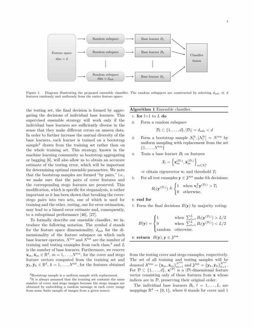
Figure 1. Diagram illustrating the proposed ensemble classifier. The random subspaces are constructed by selecting dsub ≪ dfeatures randomly and uniformly from the entire feature space.

the testing set, the final decision is formed by aggre-gating the decisions of individual base learners. Thissupervised ensemble strategy will work only if theindividual base learners are sufficiently diverse in thesense that they make different errors on unseen data.In order to further increase the mutual diversity of thebase learners, each learner is trained on a bootstrapsample2 drawn from the training set rather than onthe whole training set. This strategy, known in themachine learning community as bootstrap aggregatingor bagging [6], will also allow us to obtain an accurateestimate of the testing error, which will be importantfor determining optimal ensemble parameters. We notethat the bootstrap samples are formed “by pairs,” i.e.,we make sure that the pairs of cover features andthe corresponding stego features are preserved. Thismodification, which is specific for steganalysis, is ratherimportant as it has been shown that breaking the cover-stego pairs into two sets, one of which is used fortraining and the other, testing, one for error estimation,may lead to a biased error estimate and, consequently,to a suboptimal performance [46], [27].

To formally describe our ensemble classifier, we in-troduce the following notation. The symbol d standsfor the feature space dimensionality, dsub for the di-mensionality of the feature subspace on which eachbase learner operates, N trn and N tst are the number oftraining and testing examples from each class,3 and Lis the number of base learners. Furthermore, we reservexm, xm ∈ R

d, m = 1, . . . , N trn, for the cover and stegofeature vectors computed from the training set andyk, yk ∈ R

d, k = 1, . . . , N tst, for the features obtained

2Bootstrap sample is a uniform sample with replacement.3It is always assumed that the training set contains the same

number of cover and stego images because the stego images areobtained by embedding a random message in each cover imagefrom some finite sample of images from a given source.

Algorithm 1 Ensemble classifier.

1: for l=1 to L do

2: Form a random subspace

Dl ⊂ {1, . . . , d}, |Dl| = dsub < d

3: Form a bootstrap sample N bl ,

∣

∣N bl

∣

∣ = N trn byuniform sampling with replacement from the set{1, . . . , N trn}

4: Train a base learner Bl on features

Xl ={

x(Dl)m , x(Dl)

m

}

m∈N b

l

⇒ obtain eigenvector vl and threshold Tl

5: For all test examples y ∈ Ytst make lth decisions:

Bl(y(Dl)) ,

{

1 when vT

l y(Dl) > Tl

0 otherwise.

6: end for

7: Form the final decisions B(y) by majority voting:

B(y) =

1 when∑L

l=1 Bl(y(Dl)) > L/2

0 when∑L

l=1 Bl(y(Dl)) < L/2

random otherwise.

8: return B(y), y ∈ Ytst

from the testing cover and stego examples, respectively.The set of all training and testing samples will be

denoted X trn = {xm, xm}Ntrn

m=1 and Ytst = {yk, yk}Ntst

k=1 .For D ⊂ {1, . . . , d}, x(D) is a |D|-dimensional featurevector consisting only of those features from x whoseindices are in D, preserving their original order.

The individual base learners Bl, l = 1, . . . , L, aremappings R

d → {0, 1}, where 0 stands for cover and 1

4

for stego. Note that, even though defined on Rd, all base

learners are trained on feature spaces of a dimensiondsub that can be chosen to be much smaller than the fulldimensionality d, which significantly lowers the com-putational complexity. Even though the performanceof individual base learners can be weak, the accuracyquickly improves after fusion and eventually levels outfor a sufficiently large L. The decision threshold of eachbase learner is adjusted to minimize the total detectionerror under equal priors on the training set:

PE = minPFA

1

2(PFA + PMD(PFA)) , (1)

where PFA, PMD are the probabilities of false alarmsand missed detection, respectively.

We recommend to implement each base learner asthe Fisher Linear Discriminant (FLD) [12] because ofits low training complexity; the most time consumingpart is forming the within-class covariance matrices andinverting their summation. Additionally, such weak andunstable classifiers desirably increase diversity.

Since the FLD is a standard classification tool, weonly describe those parts of it that are relevant for theensemble classifier. The lth base learner is trained onthe set

{

x(Dl)i , x

(Dl)i |i ∈ N b

l

}

, where Dl ⊂ {1, . . . , d},

|Dl| = dsub is randomly selected subset and N bl is a

bootstrap sample drawn from the set {1, . . . , N trn},|N b

l | = N trn. Each base learner is fully described usingthe generalized eigenvector

vl = (SW + λI)−1(µ− µ), (2)

where µ, µ ∈ Rdsub are the means of each class

µ =1

N trn

∑

m∈N b

l

x(Dl)m , µ =

1

N trn

∑

m∈N b

l

x(Dl)m , (3)

SW =∑

m

(x(Dl)m −µ)(x(Dl)

m −µ)T+(x(Dl)m −µ)(x(Dl)

m −µ)T

(4)is the within-class scatter matrix, and λ is a stabilizingparameter to make the matrix SW +λI positive definiteand thus avoid problems with numerical instability inpractice when SW is singular or ill-conditioned.4

For a test feature y ∈ Ytst, the lth base learnerreaches its decision by computing the projectionvT

l y(Dl) and comparing it to a threshold (previouslyadjusted to meet a desired performance criterion). Af-ter collecting all L decisions, the final classifier outputis formed by combining them using an unweighted(majority) voting strategy – the sum of the individual

4The parameter λ can be either fixed to a small constantvalue (e.g., λ = 10−10) or dynamically increased once numericalinstability is detected.

votes is compared to the decision threshold L/2. Wenote that this threshold may be adjusted within theinterval [0, L] in order to control the importance of thetwo different types of errors or to obtain the wholereceiver operating characteristic (ROC curve). In allexperiments in this paper, we adjust the thresholdto L/2 as PE is nowadays considered standard forevaluating the accuracy of steganalyzers in practice.

The pseudo-code for the entire ensemble classifier isdescribed in Algorithm 1, while Figure 1 shows its high-level conceptual diagram. The classifier depends on twoparameters, dsub and L, which are determined usingalgorithms from Section II-C.

B. Illustrative example

Before finishing the description of the ensemble clas-sifier with procedures for automatic determination ofdsub and L, we include a simple illustrative exampleto demonstrate the effect of the parameters on per-formance. We do so for the steganographic algorithmnsF5 (no-shrinkage F5) [20] as a modern representativeof steganographic schemes for the JPEG domain, usinga simulation of its embedding impact if optimal wet-paper codes were used.5

The image source is the CAMERA database con-taining 6,500 JPEG images originally acquired in theirRAW format taken by 22 digital cameras, resized sothat the smaller size is 512 pixels with aspect ratio pre-served, converted to grayscale, and finally compressedwith JPEG quality factor 75 using Matlab’s commandimwrite. The images were randomly divided into twohalves for training and testing, respectively.

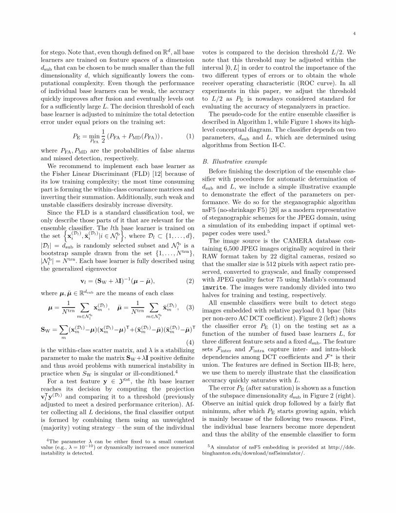
All ensemble classifiers were built to detect stegoimages embedded with relative payload 0.1 bpac (bitsper non-zero AC DCT coefficient). Figure 2 (left) showsthe classifier error PE (1) on the testing set as afunction of the number of fused base learners L, forthree different feature sets and a fixed dsub. The featuresets Finter and Fintra capture inter- and intra-blockdependencies among DCT coefficients and F∗ is theirunion. The features are defined in Section III-B; here,we use them to merely illustrate that the classificationaccuracy quickly saturates with L.

The error PE (after saturation) is shown as a functionof the subspace dimensionality dsub in Figure 2 (right).Observe an initial quick drop followed by a fairly flatminimum, after which PE starts growing again, whichis mainly because of the following two reasons. First,the individual base learners become more dependentand thus the ability of the ensemble classifier to form

5A simulator of nsF5 embedding is provided at http://dde.binghamton.edu/download/nsf5simulator/.

5

0 20 40 60 80 100

0.20

0.25

0.30

0.35

0.40Finter (dsub = 200)

Fintra (dsub = 200)

F∗ (dsub = 500)

L

PE

Dependence on L

0 500 1000 1500 2000 25000

0.10

0.20

0.30

0.40

0.50

Finter

Fintra

F∗

dsub

PE

Dependence on dsub

Figure 2. Left: Detection error PE quickly saturates with the number of fused learners L. Right: The detection error after saturationas a function of dsub. The dots represent out-of-bag error estimates EOOB (see Section II-C). Feature sets considered: Finter, Fintra,and F∗ with dimensionalities 1550, 2375, and 3925 (see Section III). Target algorithm: nsF5 with payload 0.1 bpac.

non-linear boundaries decreases. Second, the individualFLDs start to suffer from overtraining as the subspacedimensionality increases while the training size remainsthe same.

C. Parameter determination

To complete the description of the classifier, wenow supply a procedure for determining dsub andL. Since each base learner Bl is trained on Xl ={x

(Dl)m , x

(Dl)m }m∈N b

l

, where N bl is a bootstrap sample

of {1, . . . , N trn} with roughly 63% of unique samples,the remaining 37% can be used for validation as Bl

provides a single vote for each x /∈ Xl. This procedurebears similarity to cross-validation in SVM training.

After n base learners are trained, each training sam-ple x ∈ X trn will collect on average 0.37 ·n predictionsthat can be fused using the majority voting strategyinto a prediction B(n)(x) ∈ {0, 1}. The following is anunbiased estimate of the testing error known as the“out-of-bag” (OOB) estimate:

E(n)OOB =

1

2N trn

Ntrn

∑

m=1

(

B(n)(xm) + 1−B(n)(xm))

.

(5)

The term comes from bagging (bootstrap aggregat-ing) which is a well-established technique for reducingthe variance of classifiers [6]. In contrast to bagging, weuse a different random subset of features for trainingeach base learner. Figure 2 (right) illustrates that

E(n)OOB is indeed an accurate estimate of the testing

error.

1) Stopping criterion for L: As is already apparentfrom Figure 2 (left), the classification accuracy satu-rates rather quickly with L. The speed of saturation,however, depends on the accuracy of individual baselearners, on the relationship between d and dsub, andis also data dependent. Therefore, we determine Ldynamically by observing the progress of the OOBestimate (5) and stop the training once the last Kmoving averages calculated from µ consecutive EOOB

values lie in an ǫ-tube:

L = arg minn

{

n;

∣

∣

∣

∣

mini∈PK (n)

Mµ(i)− maxi∈PK (n)

Mµ(i)

∣

∣

∣

∣

< ǫ

}

,

(6)where

Mµ(i) =1

µ

i∑

j=i−µ+1

E(j)OOB (7)

and PK(n) = {n − K, . . . , n}. The parameters K, µ,and ǫ are user-defined and control the trade-off betweencomputational complexity and optimality. In all ourexperiments in this paper, we fixed K = 50, µ = 5,and ǫ = 0.005. According to our experiments, thischoice of the parameters works universally for differentsteganalysis tasks, i.e., for both small and large valuesof d and dsub, for a wide range of payloads (low and highEOOB values), and different steganographic algorithms.

Note that while E(L)OOB is formed by fusing 0.37 · L

decisions (on average), the predictions on testing sam-ples will be formed by fusing all L decisions. The finalout-of-bag estimate meeting the criterion (6) will be

denoted EOOB ≡ E(L)OOB.

2) Subspace dimension dsub: Since the classifica-tion accuracy is fairly insensitive to dsub around its

6

minimum (Figure 2 (right)), most simple “educatedguesses” of dsub give already near-optimal performance,which is important for obtaining quick insights for theanalyst. Having said this, we now supply a formalprocedure for automatic determination of dsub. BecausePE(dsub) is unimodal in dsub, the minimum can befound through a one-dimensional search over dsub us-ing EOOB(dsub) as an estimate of PE(dsub). Since thematrix inversion in (2) requires O(d3

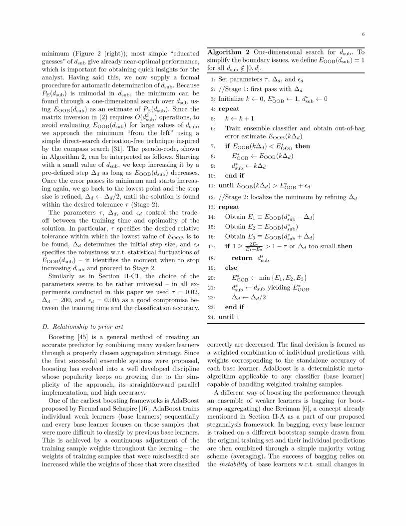
sub) operations, toavoid evaluating EOOB(dsub) for large values of dsub,we approach the minimum “from the left” using asimple direct-search derivation-free technique inspiredby the compass search [31]. The pseudo-code, shownin Algorithm 2, can be interpreted as follows. Startingwith a small value of dsub, we keep increasing it by apre-defined step ∆d as long as EOOB(dsub) decreases.Once the error passes its minimum and starts increas-ing again, we go back to the lowest point and the stepsize is refined, ∆d ← ∆d/2, until the solution is foundwithin the desired tolerance τ (Stage 2).

The parameters τ , ∆d, and ǫd control the trade-off between the training time and optimality of thesolution. In particular, τ specifies the desired relativetolerance within which the lowest value of EOOB is tobe found, ∆d determines the initial step size, and ǫd

specifies the robustness w.r.t. statistical fluctuations ofEOOB(dsub) – it identifies the moment when to stopincreasing dsub and proceed to Stage 2.

Similarly as in Section II-C1, the choice of theparameters seems to be rather universal – in all ex-periments conducted in this paper we used τ = 0.02,∆d = 200, and ǫd = 0.005 as a good compromise be-tween the training time and the classification accuracy.

D. Relationship to prior art

Boosting [45] is a general method of creating anaccurate predictor by combining many weaker learnersthrough a properly chosen aggregation strategy. Sincethe first successful ensemble systems were proposed,boosting has evolved into a well developed disciplinewhose popularity keeps on growing due to the sim-plicity of the approach, its straightforward parallelimplementation, and high accuracy.

One of the earliest boosting frameworks is AdaBoostproposed by Freund and Schapire [16]. AdaBoost trainsindividual weak learners (base learners) sequentiallyand every base learner focuses on those samples thatwere more difficult to classify by previous base learners.This is achieved by a continuous adjustment of thetraining sample weights throughout the learning – theweights of training samples that were misclassified areincreased while the weights of those that were classified

Algorithm 2 One-dimensional search for dsub. Tosimplify the boundary issues, we define EOOB(dsub) = 1for all dsub /∈ [0, d].

1: Set parameters τ , ∆d, and ǫd

2: //Stage 1: first pass with ∆d

3: Initialize k ← 0, E∗OOB ← 1, d∗

sub ← 0

4: repeat

5: k ← k + 1

6: Train ensemble classifier and obtain out-of-bagerror estimate EOOB(k∆d)

7: if EOOB(k∆d) < E∗OOB then

8: E∗OOB ← EOOB(k∆d)

9: d∗sub ← k∆d

10: end if

11: until EOOB(k∆d) > E∗OOB + ǫd

12: //Stage 2: localize the minimum by refining ∆d

13: repeat

14: Obtain E1 ≡ EOOB(d∗sub −∆d)

15: Obtain E2 ≡ EOOB(d∗sub)

16: Obtain E3 ≡ EOOB(d∗sub + ∆d)

17: if 1 ≥ 2E2

E1+E3> 1− τ or ∆d too small then

18: return d∗sub

19: else

20: E∗OOB ← min {E1, E2, E3}

21: d∗sub ← dsub yielding E∗

OOB

22: ∆d ← ∆d/2

23: end if

24: until 1

correctly are decreased. The final decision is formed asa weighted combination of individual predictions withweights corresponding to the standalone accuracy ofeach base learner. AdaBoost is a deterministic meta-algorithm applicable to any classifier (base learner)capable of handling weighted training samples.

A different way of boosting the performance throughan ensemble of weaker learners is bagging (or boot-strap aggregating) due Breiman [6], a concept alreadymentioned in Section II-A as a part of our proposedsteganalysis framework. In bagging, every base learneris trained on a different bootstrap sample drawn fromthe original training set and their individual predictionsare then combined through a simple majority votingscheme (averaging). The success of bagging relies onthe instability of base learners w.r.t. small changes in

7

the training set. An important by-product of baggingis the ability to continuously monitor the testing errorestimate (OOB).

The random forest [7] is an extended version ofbagging in the sense that it also trains individual baselearners on bootstrap samples of the training set. Thebase learners are, however, additionally randomized bymaking them dependent on a random vector that isdrawn independently and from one fixed distribution.In [7], each base learner is a decision tree whose split-ting variables are chosen randomly as a small subsetof the original variables. The final prediction is againformed as a majority vote. This additional random-ization introduces instability (and thus diversity) tothe individual base learners and substantially speeds-up the training. On the other hand, the accuracyof individual base learners decreases, which is to beexpected. However, it turns out that the combinedprediction generally yields comparable or even betterresults than bagging or AdaBoost. We would like tostress that unlike in AdaBoost, the random forest treatsindividual base learners equally in forming the finaldecision – this is because all the base learners weregenerated using the same random procedure.

The steganalysis system proposed in Section II-Acould be categorized as a random forest with the FLDas a base learner. The random component is in thefeature subspace generation and is a crucial part ofthe system as using the full feature space would becomputationally intractable due to high feature dimen-sionality.

The idea of forming random subspaces from theoriginal feature space is not new and is known un-der different names. Decision forests [24], attributebagging [9], CERP (Classification by Ensembles fromRandom Partitions) [1], or the recently proposed RSE(Random Subsample Ensemble) [47] are all ensemble-based classifiers sampling the feature space prior baselearner training to either increase the diversity amongclassifiers or reduce the original high dimension tomanageable values.

Most ensemble systems described in the literatureuse base learners implemented as classification treeseven though other classifiers may be used. For example,SVMs are used as base learners in [33], while in [2] aset of different base learners are compared, includinglogistic regression, L-SVM, and FLD. Our decision toselect the FLD was based on numerous experiments weperformed and will be discussed in more detail in thenext section. Briefly, FLDs are very fast and providedoverall good performance when combined together intoa final vote.

Besides ensemble classification, there exist numerousother well-developed strategies for reducing the train-ing complexity. One popular choice are dimensionalityreduction techniques that can be either unsupervised(PCA) or supervised (e.g., feature selection [34]) ap-plied prior to classification as a part of the feature pre-processing. However, such methods are rarely suitablefor applications in steganalysis when no small subsetof features can deliver performance similar to the full-dimensional case. The dimensionality reduction andclassification can also be performed simultaneouslyeither by minimizing an appropriately constructed sin-gle objective function directly (SVDM [38]) or byconstructing an iterative algorithm for dimensionalityreduction with a classification feedback after every it-eration. In machine learning, these methods are knownas embedded and wrapper methods [34].

Finally, the idea of using a committee of detectorsfor steganalysis appeared in [25]. However, the focusof the work was elsewhere – several classifiers weretrained individually to detect different steganographicmethods and their fusion was shown to outperform asingle classifier trained on a mixture of stego imagescreated by those methods.

E. Discussion

To the best of our knowledge, a fully automatizedframework combining random feature subspaces andbagging into a random forest classifier, together withan efficient utilization of out-of-bag error estimates forstopping criterion and the search for the optimal valueof the subspace dimension is a novel contribution notonly in the field of steganalysis, but also in the en-semble classification literature. The ensemble classifieras described in Section II provided the best overallperformance and complexity among many differentversions we have investigated. In particular, we studiedwhether it is possible to improve the performance byselecting the features randomly but non-uniformly andwe tested other base learners and aggregation rules forthe decision fusion. We also tried to replace baggingwith cross-validation and to incorporate the ideas ofAdaBoost [16] into the framework. Even though noneof these modifications brought an improvement, webelieve they deserve to be commented on and wediscuss them in this section.

Depending on the feature set and the steganographicalgorithm, certain features react more sensitively toembedding than others. Thus, it seemingly makessense to try improve the performance by selecting themore influential features more frequently instead ofuniformly at random. We tested biasing the random

8

selection to features with a higher individual Fisherratio. However, any deviation from the uniform dis-tribution lead to a drop in the performance of theentire ensemble. This is likely because biased selectionof features decreases the diversity of the individual baselearners. The problem of optimum trade-off betweendiversity and accuracy of the base learners is notcompletely resolved in the ensemble literature [36], [8]and we refrain from further analyzing this importantissue in this paper.

Next, we investigated whether base learners otherthan FLDs can improve the performance. In particular,we tested linear SVMs (L-SVMs), kernelized FLDs [37],decision trees, naive Bayesian classifiers, and logisticregression. In summary, none of these choices proveda viable alternative to the FLD. Decision trees wereunsuitable due to the fact that in steganalysis it isunlikely to find a small set of influential features (unlessthe steganography has some basic weakness). All fea-tures are rather weak and only provide detection whenconsidered as a whole or in large subsets. Interestingly,the ensemble with kernelized FLD, L-SVM, and logis-tic regression had performance comparable to FLDs,even though the individual accuracies of base learnerswere higher. Additionally, the training complexity ofthese alternative base learners was much higher. Also,unlike FLD, both L-SVM and kernelized FLD requirepre-scaling of features and a parameter search, whichfurther increases the training time.

The last element we tested was the aggregationrule. The voting as described in Algorithm 1 could bereplaced by more sophisticated rules [32]. For example,when the decision boundary is a hyperplane, one cancompute the projections of the test feature vector onthe normal vector of each base learner and thresholdtheir sum over all base learners. Alternatively, onecould take the sum of log-likelihoods of each projectionafter fitting models to the projections of cover and stegotraining features (the projections are well-modeled by aGuassian distribution). We observed, however, that allthree fusion strategies gave essentially identical results.Thus, we selected the simplest rule – the majorityvoting as our final choice.

Apart from optimizing individual components of thesystem, we also tried two alternative designs of theframework as a whole. First, we replaced the bootstrap-ping and out-of-bag error estimation with k-fold cross-validation. This modification yielded similar results asthe original system based on OOB estimates.

The second direction of our efforts was to incorporatethe ideas of AdaBoost. There are several ways of doingso. We can boost individual FLDs using AdaBoost and

use them as base learners for the ensemble framework.Alternatively, we could use the whole ensemble asdescribed in Section II as a base learner for AdaBoost.Both options, however, dramatically increase the com-plexity of the system. Additionally, we would lose theconvenience of estimating the testing error simply asOOB estimates.

Another option is to apply AdaBoost into the frame-work directly by adjusting the training sample weightsas the training progresses and replacing the final ma-jority voting with a weighted sum of the individual pre-dictions. There are, however, two complications: everybase learner is trained in a different feature space andon different training samples. An appealing (and sim-ple) way of resolving these problems is to use the cross-validation variant of the ensemble mentioned above.Using k-fold cross-validation, the entire process couldbe viewed as training k parallel ensemble systems, eachof them trained on a different (but fixed) trainingset consisting of k − 1 folds. AdaBoost could thenbe used to boost each of these k sub-machines, whilethe testing error estimation (and thus the automaticensemble parameter search procedure) could be carriedout through the folds left out.

We implemented this modified system and subjectedit to numerous comparative experiments under differ-ent steganalysis scenarios. However, no performancegain has been achieved. Therefore, we conclude that theimplementation as a random forest built from equallyweighted FLDs trained on different random subspacesis the overall best approach among those we tested.

More details about our experiments with k-foldcross-validation and AdaBoost appear in the technicalreport [26], where we summarize all the comparativeresults mentioned in the previous paragraphs.

III. EXAMPLE: STEGANALYSIS IN JPEGDOMAIN

We now demonstrate the power and advantages ofthe proposed approach on a specific tell-tale exampleof how a steganalyst might use ensemble classifiers toassemble a feature set in practice and build a classifier.While the detector built here markedly outperformsexisting state of the art, we stress that the purpose ofthis illustrative exposition is not to optimize the featureset design w.r.t. a specific algorithm and cover source.We intend to study this important topic as part of ourfuture work.

A. Co-occurrences

Capturing dependencies among pairs of individualDCT coefficients through co-occurrence matrices is a

9

0 1 2 3 4 5 6 7

0

1

2

3

4

5

6

7

C12(0, 1)

C23(1, 1)C20(−1, 1)

C01(0, 8)

C40(0, 2)

8×8 DCT block

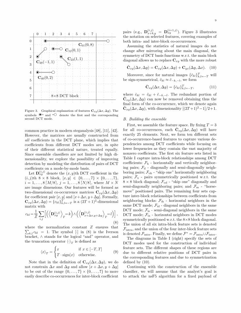
Figure 3. Graphical explanation of features Cxy(∆x, ∆y). The

symbols and denote the first and the correspondingsecond DCT mode.

common practice in modern steganalysis [48], [11], [42].However, the matrices are usually constructed fromall coefficients in the DCT plane, which implies thatcoefficients from different DCT modes are, in spiteof their different statistical nature, treated equally.Since ensemble classifiers are not limited by high di-mensionality, we explore the possibility of improvingdetection by modeling the distribution of pairs of DCTcoefficients on a mode-by-mode basis.

Let D(i,j)xy denote the (x, y)th DCT coefficient in the

(i, j)th 8 × 8 block, [x, y] ∈ {0, . . . , 7} × {0, . . . , 7},i = 1, . . . , 8 ⌈M/8⌉, j = 1, . . . , 8 ⌈N/8⌉, where M × Nare image dimensions. Our features will be formed astwo-dimensional co-occurrence matrices Cxy(∆x, ∆y)for coefficient pair [x, y] and [x+∆x, y+∆y]. Formally,Cxy(∆x, ∆y) = {ckl}T

k,l=−T is a (2T + 1)2-dimensionalmatrix with

ckl =1

Z

∑

i,j

[(⟨

D(i,j)xy

⟩

T=k

)

∧(⟨

D(i,j)x+∆x,y+∆y

⟩

T= l

)]

,

(8)where the normalization constant Z ensures that∑

k,l ckl = 1. The symbol [·] in (8) is the Iversonbracket, ∧ stands for the logical “and” operator, andthe truncation operator 〈·〉T is defined as

〈x〉T =

{

x if x ∈ [−T, T ]

T · sign(x) otherwise.(9)

Note that in the definition of Cxy(∆x, ∆y), we donot constrain ∆x and ∆y and allow [x + ∆x, y + ∆y]to be out of the range {0, . . . , 7} × {0, . . . , 7} to moreeasily describe co-occurrences for inter-block coefficient

pairs (e.g., D(i,j)x+8,y = D

(i+1,j)xy ). Figure 3 illustrates

the notation on selected features, covering examples ofboth intra- and inter-block co-occurrences.

Assuming the statistics of natural images do notchange after mirroring about the main diagonal, thesymmetry of DCT basis functions w.r.t. the main blockdiagonal allows us to replace Cxy with the more robust

Cxy(∆x, ∆y) = Cxy(∆x, ∆y) + Cyx(∆y, ∆x). (10)

Moreover, since for natural images {ckl}Tk,l=−T will

be sign-symmetrical, ckl ≈ c−k,−l, we form

Cxy(∆x, ∆y) = {ckl}Tk,l=−T , (11)

where ckl = ckl + c−k,−l. The redundant portion ofCxy(∆x, ∆y) can now be removed obtaining thus thefinal form of the co-occurrence, which we denote againCxy(∆x, ∆y), with dimensionality [(2T +1)2−1]/2+1.

B. Building the ensemble

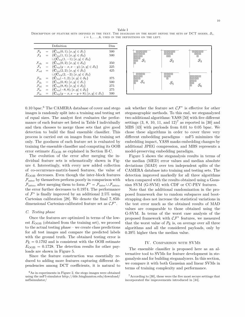
First, we assemble the feature space. By fixing T = 3for all co-occurrences, each Cxy(∆x, ∆y) will haveexactly 25 elements. Next, we form ten different setsof co-occurrence-based features to capture various de-pendencies among DCT coefficients while focusing onlower frequencies as they contain the vast majority ofnonzero coefficients. The first six feature sets listed inTable I capture intra-block relationships among DCTcoefficients: Fh - horizontally and vertically neighbor-ing pairs; Fd - diagonally and semi-diagonally neigh-boring pairs; Foh - “skip one” horizontally neighboringpairs; Fx - pairs symmetrically positioned w.r.t. the8 × 8 block diagonal; Fod - “skip one” diagonally andsemi-diagonally neighboring pairs; and Fm - “horse-move” positioned pairs. The remaining four sets cap-ture inter-block relationships between coefficients fromneighboring blocks: Fih - horizontal neighbors in thesame DCT mode; Fid - diagonal neighbors in the sameDCT mode; Fis - semi-diagonal neighbors in the sameDCT mode; Fix - horizontal neighbors in DCT modessymmetrically positioned w.r.t. the 8×8 block diagonal.The union of all six intra-block feature sets is denotedFintra, and the union of the four inter-block feature setsis denoted Finter. Finally, we define F∗ = Fintra∪Finter.

The diagrams in Table I (right) specify the sets ofDCT modes used for the construction of individualfeature sets. The different shapes of these regions aredue to different relative positions of DCT pairs inthe corresponding features and due to symmetrizationdefined by (10).

Continuing with the construction of the ensembleclassifier, we will assume that the analyst’s goal isto attack the nsF5 algorithm for a fixed payload of

10

Table IDescription of feature sets defined in the text. The diagrams on the right define the sets of DCT modes, Si,

i = 1, . . . , 6, used in the definitions on the left.

Definition Dim

Fh = {Cxy(0, 1); [x, y] ∈ S1} 500Fd = {Cxy(1, 1); [x, y] ∈ S2} 500

∪{Cxy(1, −1); [x, y] ∈ S3}Foh = {Cxy(0, 2); [x, y] ∈ S4} 350Fx = {Cxy(y − x, x − y); [x, y] ∈ S3} 225Fod = {Cxy(2, 2); [x, y] ∈ S5} 425

∪{Cxy(2, −2); [x, y] ∈ S3}Fm = {Cxy(−1, 2); [x, y] ∈ S6} 375Fih = {Cxy(0, 8); [x, y] ∈ S1} 500Fid = {Cxy(8, 8); [x, y] ∈ S2} 275Fis = {Cxy(−8, 8); [x, y] ∈ S2} 275Fix = {Cxy(y − x, x − y + 8); [x, y] ∈ S1} 500

S1 S2 S3

S4 S5S6

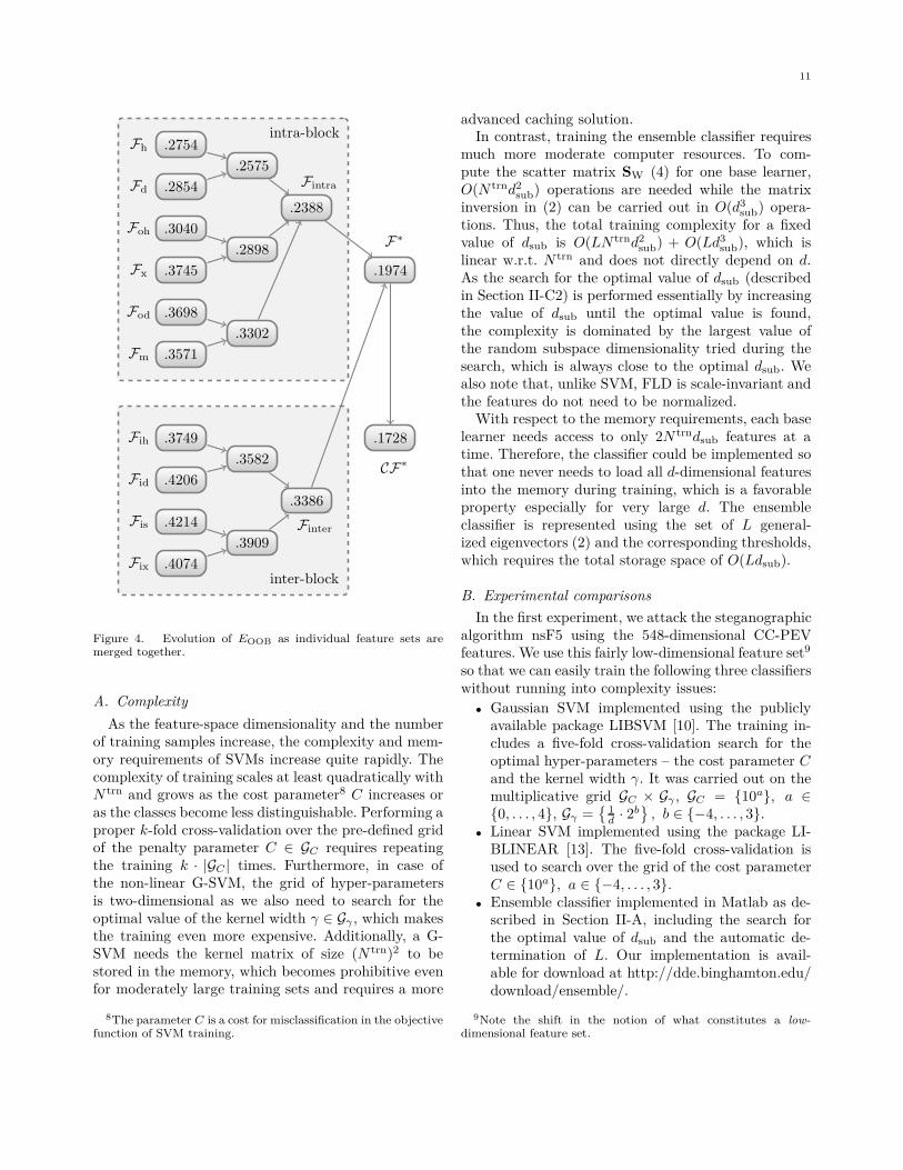
0.10 bpac.6 The CAMERA database of cover and stegoimages is randomly split into a training and testing setof equal sizes. The analyst first evaluates the perfor-mance of each feature set listed in Table I individuallyand then chooses to merge those sets that give gooddetection to build the final ensemble classifier. Thisprocess is carried out on images from the training setonly. The goodness of each feature set is evaluated bytraining the ensemble classifier and computing its OOBerror estimate EOOB as explained in Section II-C.

The evolution of the error after merging the in-dividual feature sets is schematically shown in Fig-ure 4. Interestingly, with every new added collectionof co-occurrence-matrix-based features, the value ofEOOB decreases. Even though the inter-block featuresFinter by themselves perform poorly in comparison withFintra, after merging them to form F∗ = Finter∪Fintra,the error further decreases to 0.1974. The performanceof F∗ is finally improved by an additional 2.5% usingCartesian calibration [28]. We denote the final 7, 850-dimensional Cartesian-calibrated feature set as CF∗.

C. Testing phase

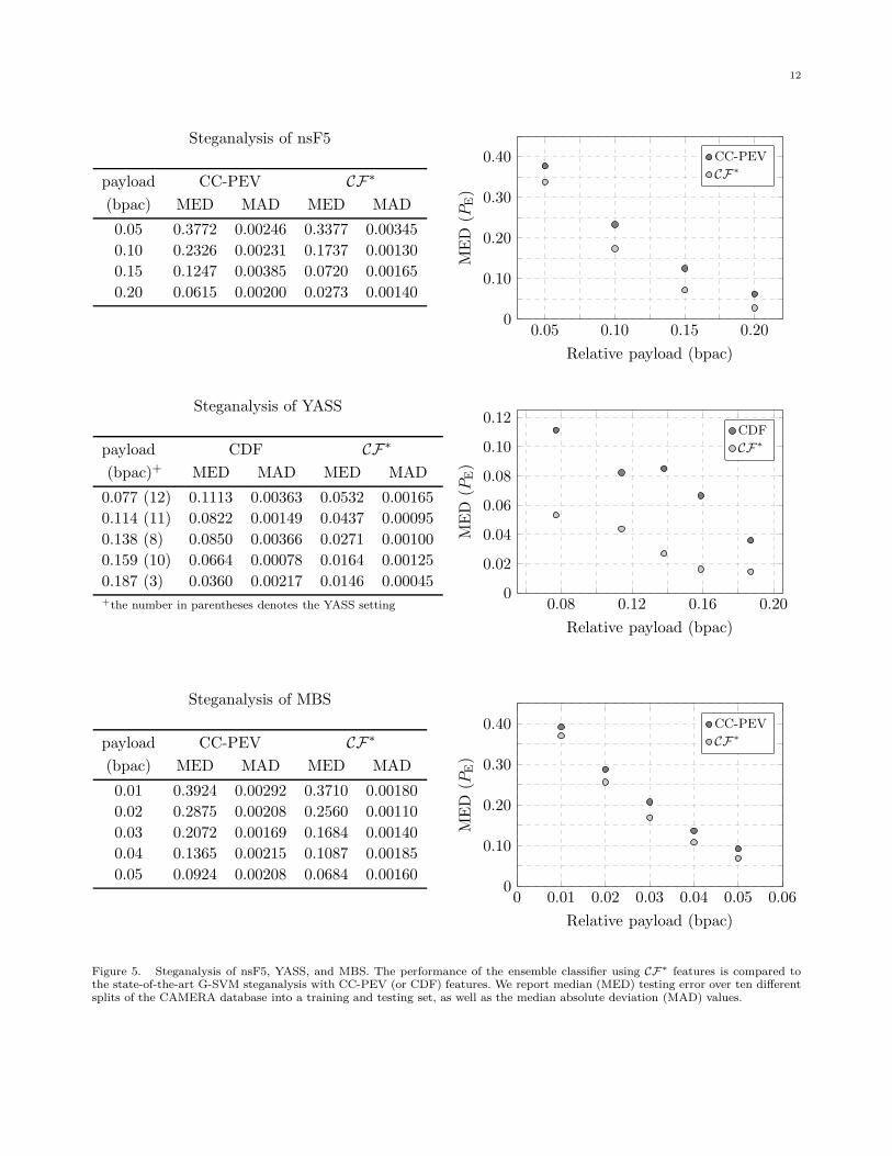
Once the features are optimized in terms of the low-est EOOB (obtained from the training set), we proceedto the actual testing phase – we create class predictionsfor all test images and compare the predicted labelswith the ground truth. The obtained testing error isPE = 0.1702 and is consistent with the OOB estimateEOOB = 0.1728. The detection results for other pay-loads are shown in Figure 5.

Since the feature construction was essentially re-duced to adding more features capturing different de-pendencies among DCT coefficients, it is natural to

6As in experiments in Figure 2, the stego images were obtainedusing the nsF5 simulator http://dde.binghamton.edu/download/nsf5simulator/

ask whether the feature set CF∗ is effective for othersteganographic methods. To this end, we steganalyzedtwo additional algorithms: YASS [50] with five differentsettings (3, 8, 10, 11, and 12)7 as reported in [30] andMBS [43] with payloads from 0.01 to 0.05 bpac. Wechose these algorithms in order to cover three verydifferent embedding paradigms – nsF5 minimizes theembedding impact, YASS masks embedding changes byadditional JPEG compression, and MBS represents amodel-preserving embedding paradigm.

Figure 5 shows the steganalysis results in terms ofthe median (MED) error values and median absolutedeviations (MAD) over ten independent splits of theCAMERA database into training and testing sets. Thedetection improved markedly for all three algorithmswhen compared with the results obtained using a Gaus-sian SVM (G-SVM) with CDF or CC-PEV features.

Note that the additional randomization in the pro-posed framework due to random subspaces and boot-strapping does not increase the statistical variations inthe test error much as the obtained results of MADvalues are comparable to those obtained using theG-SVM. In terms of the worst case analysis of theproposed framework with CF∗ features, we measuredthat the worst value of PE is, on average over all threealgorithms and all the considered payloads, only by0.39% higher then the median value.

IV. Comparison with SVMs

The ensemble classifier is proposed here as an al-ternative tool to SVMs for feature development in ste-ganalysis and for building steganalyzers. In this section,we compare it with both Gaussian and linear SVMs interms of training complexity and performance.

7According to [30], these were the five most secure settings thatincorporated the improvements introduced in [44].

11

intra-block

inter-block

.2754

.2854

.3040

.3745

.3698

.3571

.3749

.4206

.4214

.4074

Fh

Fd

Foh

Fx

Fod

Fm

Fih

Fid

Fis

Fix

.2575

.2898

.3302

.3582

.3909

.2388

.3386

.1974

.1728

F∗

CF∗

Finter

Fintra

Figure 4. Evolution of EOOB as individual feature sets aremerged together.

A. Complexity

As the feature-space dimensionality and the numberof training samples increase, the complexity and mem-ory requirements of SVMs increase quite rapidly. Thecomplexity of training scales at least quadratically withN trn and grows as the cost parameter8 C increases oras the classes become less distinguishable. Performing aproper k-fold cross-validation over the pre-defined gridof the penalty parameter C ∈ GC requires repeatingthe training k · |GC | times. Furthermore, in case ofthe non-linear G-SVM, the grid of hyper-parametersis two-dimensional as we also need to search for theoptimal value of the kernel width γ ∈ Gγ , which makesthe training even more expensive. Additionally, a G-SVM needs the kernel matrix of size (N trn)2 to bestored in the memory, which becomes prohibitive evenfor moderately large training sets and requires a more

8The parameter C is a cost for misclassification in the objectivefunction of SVM training.

advanced caching solution.In contrast, training the ensemble classifier requires

much more moderate computer resources. To com-pute the scatter matrix SW (4) for one base learner,O(N trnd2

sub) operations are needed while the matrixinversion in (2) can be carried out in O(d3

sub) opera-tions. Thus, the total training complexity for a fixedvalue of dsub is O(LN trnd2

sub) + O(Ld3sub), which is

linear w.r.t. N trn and does not directly depend on d.As the search for the optimal value of dsub (describedin Section II-C2) is performed essentially by increasingthe value of dsub until the optimal value is found,the complexity is dominated by the largest value ofthe random subspace dimensionality tried during thesearch, which is always close to the optimal dsub. Wealso note that, unlike SVM, FLD is scale-invariant andthe features do not need to be normalized.

With respect to the memory requirements, each baselearner needs access to only 2N trndsub features at atime. Therefore, the classifier could be implemented sothat one never needs to load all d-dimensional featuresinto the memory during training, which is a favorableproperty especially for very large d. The ensembleclassifier is represented using the set of L general-ized eigenvectors (2) and the corresponding thresholds,which requires the total storage space of O(Ldsub).

B. Experimental comparisons

In the first experiment, we attack the steganographicalgorithm nsF5 using the 548-dimensional CC-PEVfeatures. We use this fairly low-dimensional feature set9

so that we can easily train the following three classifierswithout running into complexity issues:

• Gaussian SVM implemented using the publiclyavailable package LIBSVM [10]. The training in-cludes a five-fold cross-validation search for theoptimal hyper-parameters – the cost parameter Cand the kernel width γ. It was carried out on themultiplicative grid GC × Gγ , GC = {10a}, a ∈{0, . . . , 4}, Gγ =

{

1d· 2b

}

, b ∈ {−4, . . . , 3}.• Linear SVM implemented using the package LI-

BLINEAR [13]. The five-fold cross-validation isused to search over the grid of the cost parameterC ∈ {10a}, a ∈ {−4, . . . , 3}.

• Ensemble classifier implemented in Matlab as de-scribed in Section II-A, including the search forthe optimal value of dsub and the automatic de-termination of L. Our implementation is avail-able for download at http://dde.binghamton.edu/download/ensemble/.

9Note the shift in the notion of what constitutes a low-dimensional feature set.

12

0.05 0.10 0.15 0.200

0.10

0.20

0.30

0.40

Relative payload (bpac)

MED

(PE)

CC-PEV

CF∗

Steganalysis of nsF5

payload CC-PEV CF∗

(bpac) MED MAD MED MAD

0.05 0.3772 0.00246 0.3377 0.00345

0.10 0.2326 0.00231 0.1737 0.00130

0.15 0.1247 0.00385 0.0720 0.00165

0.20 0.0615 0.00200 0.0273 0.00140

0.160.120.08 0.200

0.02

0.04

0.06

0.08

0.10

0.12

Relative payload (bpac)

MED

(PE)

CDF

CF∗

Steganalysis of YASS

payload CDF CF∗

(bpac)+ MED MAD MED MAD

0.077 (12) 0.1113 0.00363 0.0532 0.00165

0.114 (11) 0.0822 0.00149 0.0437 0.00095

0.138 (8) 0.0850 0.00366 0.0271 0.00100

0.159 (10) 0.0664 0.00078 0.0164 0.00125

0.187 (3) 0.0360 0.00217 0.0146 0.00045+the number in parentheses denotes the YASS setting

0 0.01 0.02 0.03 0.04 0.05 0.060

0.10

0.20

0.30

0.40

Relative payload (bpac)

MED

(PE)

CC-PEV

CF∗

Steganalysis of MBS

payload CC-PEV CF∗

(bpac) MED MAD MED MAD

0.01 0.3924 0.00292 0.3710 0.00180

0.02 0.2875 0.00208 0.2560 0.00110

0.03 0.2072 0.00169 0.1684 0.00140

0.04 0.1365 0.00215 0.1087 0.00185

0.05 0.0924 0.00208 0.0684 0.00160

Figure 5. Steganalysis of nsF5, YASS, and MBS. The performance of the ensemble classifier using CF∗ features is compared tothe state-of-the-art G-SVM steganalysis with CC-PEV (or CDF) features. We report median (MED) testing error over ten differentsplits of the CAMERA database into a training and testing set, as well as the median absolute deviation (MAD) values.

13

Splitting the CAMERA database in two halves – onefor training and the other half for testing, a set ofstego images was created for each relative payloadα ∈ {0.05, 0.1, 0.15, 0.2} bpac. Table II shows thedetection accuracy and the training time of all threeclassifiers. The time was measured on a computer withthe AMD Opteron 275 processor running at 2.2 GHz.

The performance of all three classifiers is very sim-ilar, suggesting that the optimal decision boundarybetween cover and stego images in the CC-PEV featurespace is linear or close to linear. Note that while thetesting errors are comparable, the time required fortraining differs substantially. While the G-SVM tookseveral hours to train, the training of L-SVMs wasaccomplished in 14–23 minutes. The ensemble classifieris clearly the fastest, taking approximately 2 minutesto train across all payloads.

With the increasing complexity and diversity of covermodels, future steganalysis must inevitably start usinglarger training sets. Our second experiment demon-strates that the computational complexity of the en-semble classifier scales much more favorably w.r.t. thetraining set size N trn.10 To this end, we fixed the pay-load to 0.10 bpac and extended the CAMERA databaseby 10, 000 images from the BOWS2 competition [4]and 9, 074 BOSSbase images [40]. Both databases wereJPEG compressed using the quality factor 75. Theresulting collection of images allowed us to increase thetraining size to N trn = 25, 000.

Table III shows the training times for different N trn.The values for the L-SVM and the ensemble classifierare averages over five independent random selections oftraining images. As the purpose of this experiment israther illustrative and the G-SVM classifier is appar-ently computationally infeasible even for relatively lowvalues of N trn, we report its training times measuredonly for a single randomly selected training set anddrop it from experiments with N trn > 5, 000 entirely.It is apparent that although the L-SVM training iscomputationally feasible even for the largest values ofN trn, the ensemble is still substantially faster and thedifference quickly grows with the training set size.

In our last experiment, we compare the performanceof the L-SVM with the ensemble classifier when a high-dimensional feature space is used for steganalysis. TheG-SVM was not included in this test due to its highcomplexity. We consider the 7, 850-dimensional featurevector CF∗ constructed in Section III and use it toattack nsF5, YASS, and MBS. This experiment revealshow well both classifiers handle the scenario when the

10The actual number of training samples is 2Ntrn as we takeboth cover and stego features.

Table IISteganalysis of nsF5 using CC-PEV features. The

running times and PE values are medians (MED) over tenindependent splits of the CAMERA database intotraining and testing sets. We also report median

absolute deviation (MAD) values for PE.

bpac Classifier PE Training timeMED MAD

0.05 G-SVM 0.3772 0.00246 7 hr 29 minL-SVM 0.3802 0.00269 23 min

Ensemble 0.3695 0.00145 2 min

0.10 G-SVM 0.2326 0.00231 6 hr 52 minL-SVM 0.2421 0.00246 27 min

Ensemble 0.2226 0.00265 3 min

0.15 G-SVM 0.1247 0.00385 5 hr 39 minL-SVM 0.1342 0.00185 26 min

Ensemble 0.1160 0.00170 3 min

0.20 G-SVM 0.0615 0.00200 4 hr 51 minL-SVM 0.0638 0.00123 27 min

Ensemble 0.0547 0.00150 3 min

Table IIIDependence of the training time on Ntrn. Target

algorithm: nsF5 with 0.10 bpac.

Ntrn G-SVM L-SVM Ensemble

1,000 33 min 5 min < 1 min2,000 2 hr 27 min 10 min 1 min3,000 5 hr 24 min 14 min 1.5 min4,000 9 hr 31 min 20 min 2 min5,000 13 hr 47 min 27 min 2 min

10,000 × 54 min 4 min

15,000 × 1 hr 23 min 5 min

20,000 × 1 hr 52 min 6 min

25,000 × 2 hr 21 min 8 min

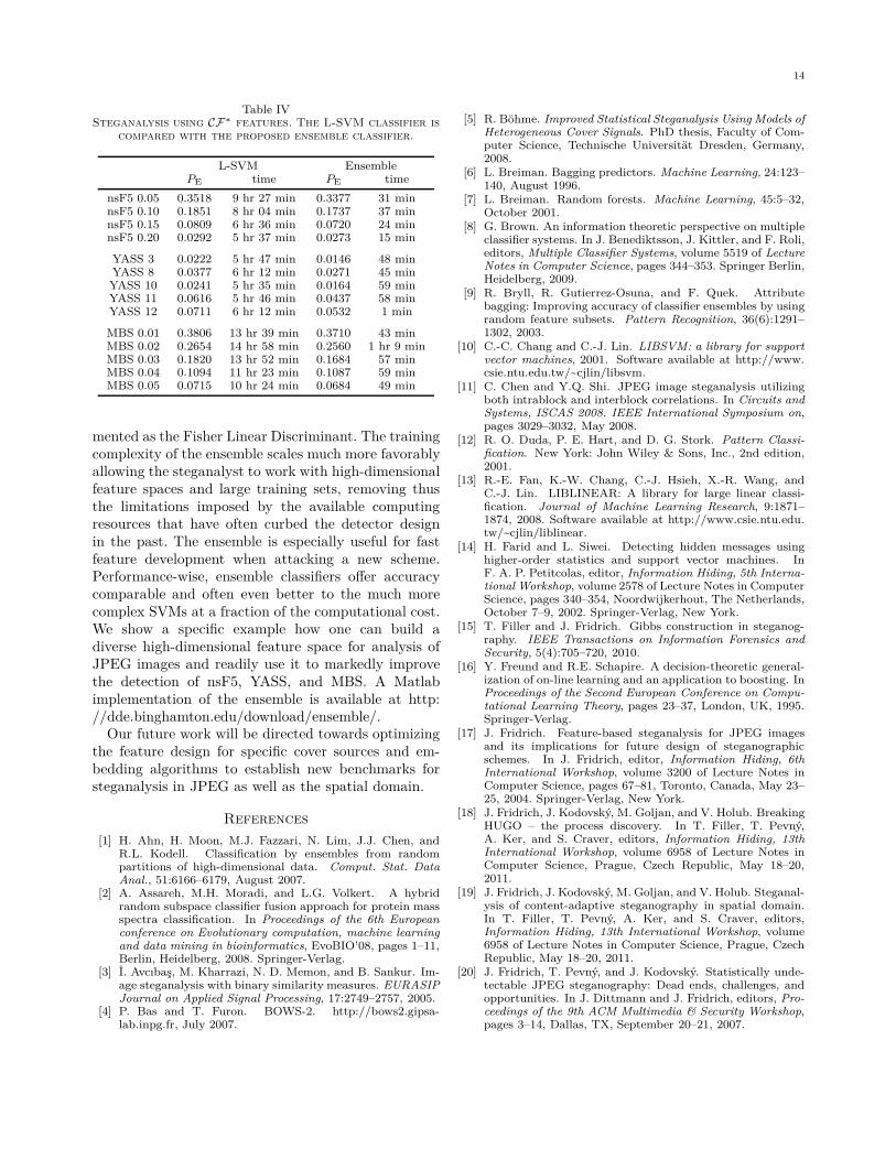
feature space dimensionality is larger than the numberof training samples. The comparison is reported inTable IV. The ensemble classifier is substantially fasterand delivers a higher accuracy for all three algorithms(the decision boundary seems to be farther from linearthan in the case of CC-PEV features).

V. SUMMARY

The current trend in steganalysis is to train classifierswith increasingly more complex cover models and largedata sets to obtain more accurate and robust detectors.The complexity of the tool-of-choice, the support vec-tor machine, however, does not scale favorably w.r.t.feature dimensionality and the training set size. Tofacilitate further development of steganalysis, we pro-pose an alternative – ensemble classifiers built by fusingdecisions of weak and unstable base learners imple-

14

Table IVSteganalysis using CF∗ features. The L-SVM classifier is

compared with the proposed ensemble classifier.

L-SVM EnsemblePE time PE time

nsF5 0.05 0.3518 9 hr 27 min 0.3377 31 minnsF5 0.10 0.1851 8 hr 04 min 0.1737 37 minnsF5 0.15 0.0809 6 hr 36 min 0.0720 24 minnsF5 0.20 0.0292 5 hr 37 min 0.0273 15 min

YASS 3 0.0222 5 hr 47 min 0.0146 48 minYASS 8 0.0377 6 hr 12 min 0.0271 45 minYASS 10 0.0241 5 hr 35 min 0.0164 59 minYASS 11 0.0616 5 hr 46 min 0.0437 58 minYASS 12 0.0711 6 hr 12 min 0.0532 1 min

MBS 0.01 0.3806 13 hr 39 min 0.3710 43 minMBS 0.02 0.2654 14 hr 58 min 0.2560 1 hr 9 minMBS 0.03 0.1820 13 hr 52 min 0.1684 57 minMBS 0.04 0.1094 11 hr 23 min 0.1087 59 minMBS 0.05 0.0715 10 hr 24 min 0.0684 49 min

mented as the Fisher Linear Discriminant. The trainingcomplexity of the ensemble scales much more favorablyallowing the steganalyst to work with high-dimensionalfeature spaces and large training sets, removing thusthe limitations imposed by the available computingresources that have often curbed the detector designin the past. The ensemble is especially useful for fastfeature development when attacking a new scheme.Performance-wise, ensemble classifiers offer accuracycomparable and often even better to the much morecomplex SVMs at a fraction of the computational cost.We show a specific example how one can build adiverse high-dimensional feature space for analysis ofJPEG images and readily use it to markedly improvethe detection of nsF5, YASS, and MBS. A Matlabimplementation of the ensemble is available at http://dde.binghamton.edu/download/ensemble/.

Our future work will be directed towards optimizingthe feature design for specific cover sources and em-bedding algorithms to establish new benchmarks forsteganalysis in JPEG as well as the spatial domain.

References

[1] H. Ahn, H. Moon, M.J. Fazzari, N. Lim, J.J. Chen, andR.L. Kodell. Classification by ensembles from randompartitions of high-dimensional data. Comput. Stat. DataAnal., 51:6166–6179, August 2007.

[2] A. Assareh, M.H. Moradi, and L.G. Volkert. A hybridrandom subspace classifier fusion approach for protein massspectra classification. In Proceedings of the 6th Europeanconference on Evolutionary computation, machine learningand data mining in bioinformatics, EvoBIO’08, pages 1–11,Berlin, Heidelberg, 2008. Springer-Verlag.

[3] İ. Avcıbaş, M. Kharrazi, N. D. Memon, and B. Sankur. Im-age steganalysis with binary similarity measures. EURASIPJournal on Applied Signal Processing, 17:2749–2757, 2005.

[4] P. Bas and T. Furon. BOWS-2. http://bows2.gipsa-lab.inpg.fr, July 2007.

[5] R. Böhme. Improved Statistical Steganalysis Using Models ofHeterogeneous Cover Signals. PhD thesis, Faculty of Com-puter Science, Technische Universität Dresden, Germany,2008.

[6] L. Breiman. Bagging predictors. Machine Learning, 24:123–140, August 1996.

[7] L. Breiman. Random forests. Machine Learning, 45:5–32,October 2001.

[8] G. Brown. An information theoretic perspective on multipleclassifier systems. In J. Benediktsson, J. Kittler, and F. Roli,editors, Multiple Classifier Systems, volume 5519 of LectureNotes in Computer Science, pages 344–353. Springer Berlin,Heidelberg, 2009.

[9] R. Bryll, R. Gutierrez-Osuna, and F. Quek. Attributebagging: Improving accuracy of classifier ensembles by usingrandom feature subsets. Pattern Recognition, 36(6):1291–1302, 2003.

[10] C.-C. Chang and C.-J. Lin. LIBSVM: a library for supportvector machines, 2001. Software available at http://www.csie.ntu.edu.tw/~cjlin/libsvm.

[11] C. Chen and Y.Q. Shi. JPEG image steganalysis utilizingboth intrablock and interblock correlations. In Circuits andSystems, ISCAS 2008. IEEE International Symposium on,pages 3029–3032, May 2008.

[12] R. O. Duda, P. E. Hart, and D. G. Stork. Pattern Classi-fication. New York: John Wiley & Sons, Inc., 2nd edition,2001.

[13] R.-E. Fan, K.-W. Chang, C.-J. Hsieh, X.-R. Wang, andC.-J. Lin. LIBLINEAR: A library for large linear classi-fication. Journal of Machine Learning Research, 9:1871–1874, 2008. Software available at http://www.csie.ntu.edu.tw/~cjlin/liblinear.

[14] H. Farid and L. Siwei. Detecting hidden messages usinghigher-order statistics and support vector machines. InF. A. P. Petitcolas, editor, Information Hiding, 5th Interna-tional Workshop, volume 2578 of Lecture Notes in ComputerScience, pages 340–354, Noordwijkerhout, The Netherlands,October 7–9, 2002. Springer-Verlag, New York.

[15] T. Filler and J. Fridrich. Gibbs construction in steganog-raphy. IEEE Transactions on Information Forensics andSecurity, 5(4):705–720, 2010.

[16] Y. Freund and R.E. Schapire. A decision-theoretic general-ization of on-line learning and an application to boosting. InProceedings of the Second European Conference on Compu-tational Learning Theory, pages 23–37, London, UK, 1995.Springer-Verlag.

[17] J. Fridrich. Feature-based steganalysis for JPEG imagesand its implications for future design of steganographicschemes. In J. Fridrich, editor, Information Hiding, 6thInternational Workshop, volume 3200 of Lecture Notes inComputer Science, pages 67–81, Toronto, Canada, May 23–25, 2004. Springer-Verlag, New York.

[18] J. Fridrich, J. Kodovský, M. Goljan, and V. Holub. BreakingHUGO – the process discovery. In T. Filler, T. Pevný,A. Ker, and S. Craver, editors, Information Hiding, 13thInternational Workshop, volume 6958 of Lecture Notes inComputer Science, Prague, Czech Republic, May 18–20,2011.

[19] J. Fridrich, J. Kodovský, M. Goljan, and V. Holub. Steganal-ysis of content-adaptive steganography in spatial domain.In T. Filler, T. Pevný, A. Ker, and S. Craver, editors,Information Hiding, 13th International Workshop, volume6958 of Lecture Notes in Computer Science, Prague, CzechRepublic, May 18–20, 2011.

[20] J. Fridrich, T. Pevný, and J. Kodovský. Statistically unde-tectable JPEG steganography: Dead ends, challenges, andopportunities. In J. Dittmann and J. Fridrich, editors, Pro-ceedings of the 9th ACM Multimedia & Security Workshop,pages 3–14, Dallas, TX, September 20–21, 2007.

15

[21] M. Goljan, J. Fridrich, and T. Holotyak. New blind steganal-ysis and its implications. In E. J. Delp and P. W. Wong,editors, Proceedings SPIE, Electronic Imaging, Security,Steganography, and Watermarking of Multimedia ContentsVIII, volume 6072, pages 1–13, San Jose, CA, January 16–19, 2006.

[22] G. Gül, A.E. Dirik, and İ. Avcıbaş. Steganalytic featuresfor JPEG compression-based perturbed quantization. IEEESignal Processing Letters, 14(3):205–208, March 2000.

[23] G. Gül and F. Kurugollu. A new methodology in steganaly-sis : Breaking highly undetactable steganograpy (HUGO).In T. Filler, T. Pevný, A. Ker, and S. Craver, editors,Information Hiding, 13th International Workshop, volume6958 of Lecture Notes in Computer Science, Prague, CzechRepublic, May 18–20, 2011.

[24] T.K. Ho. The random subspace method for constructingdecision forests. IEEE Transactions on Pattern Analysisand Machine Intelligence, 20:832–844, 1998.

[25] M. Kharrazi, H.T. Sencar, and N. Memon. Improvingsteganalysis by fusion techniques: A case study with imagesteganography. LNCS Transactions on Data Hiding andMultimedia Security I, 4300:123–137, 2006.

[26] J. Kodovský. Ensemble classification in steganalysis – cross-validation and AdaBoost. Technical report, BinghamtonUniversity, August 2011.

[27] J. Kodovský. On dangers of cross-validation in steganalysis.Technical report, Binghamton University, August 2011.

[28] J. Kodovský and J. Fridrich. Calibration revisited. InJ. Dittmann, S. Craver, and J. Fridrich, editors, Proceedingsof the 11th ACM Multimedia & Security Workshop, pages63–74, Princeton, NJ, September 7–8, 2009.

[29] J. Kodovský and J. Fridrich. Steganalysis in high dimen-sions: Fusing classifiers built on random subspaces. InN. D. Memon, E. J. Delp, P. W. Wong, and J. Dittmann,editors, Proceedings SPIE, Electronic Imaging, Security andForensics of Multimedia XIII, volume 7880, pages OL 1–13,San Francisco, CA, January 23–26, 2011.

[30] J. Kodovský, T. Pevný, and J. Fridrich. Modern steganalysiscan detect YASS. In N. D. Memon, E. J. Delp, P. W.Wong, and J. Dittmann, editors, Proceedings SPIE, Elec-tronic Imaging, Security and Forensics of Multimedia XII,volume 7541, pages 02–01–02–11, San Jose, CA, January17–21, 2010.

[31] T.G. Kolda, R.M. Lewis, and V. Torczon. Optimizationby direct search: New perspectives on some classical andmodern methods. SIAM Review, 45:385–482, 2003.

[32] L. I. Kuncheva. Combining Pattern Classifiers: Methods andAlgorithms. Wiley-Interscience, 2004.

[33] L.I. Kuncheva, J.J. Rodriguez Diez, C.O. Plumpton, D.E.J.Linden, and S.J. Johnston. Random subspace ensembles forfMRI classification. IEEE Transactions on Medical Imaging,29:531–542, 2010.

[34] T.N. Lal, O. Chapelle, J. Weston, and A. Elisseeff. Em-bedded methods. In I. Guyon, S. Gunn, M. Nikravesh,and L. A. Zadeh, editors, Feature Extraction: Foundationsand Applications, Studies in Fuzziness and Soft Computing,pages 137–165. Physica-Verlag, Springer, 2006.

[35] W. Luo, F. Huang, and J. Huang. Edge adaptiveimage steganography based on LSB matching revisited.IEEE Transactions on Information Forensics and Security,5(2):201–214, June 2010.

[36] J. Meynet and J.-P. Thiran. Information theoretic com-bination of classifiers with application to AdaBoost. InM. Haindl, J. Kittler, and F. Roli, editors, Multiple Clas-sifier Systems, volume 4472 of Lecture Notes in ComputerScience, pages 171–179. Springer Berlin / Heidelberg, 2007.

[37] S. Mika, G. Ratsch, J. Weston, B. Schölkopf, and K.R.Mullers. Fisher discriminant analysis with kernels. InProceedings of the 1999 IEEE Signal Processing Society

Workshop Neural Networks for Signal Processing IX, pages41–48, Madison, WI, August 1999.

[38] F. Pereira and G. Gordon. The support vector decompo-sition machine. In Proceedings of the 23rd internationalconference on Machine learning, ICML ’06, pages 689–696,Pittsburgh, PA, 2006.

[39] T. Pevný, P. Bas, and J. Fridrich. Steganalysis by subtrac-tive pixel adjacency matrix. IEEE Transactions on Infor-mation Forensics and Security, 5(2):215–224, June 2010.

[40] T. Pevný, T. Filler, and P. Bas. Break Our SteganographicSystem, http://boss.gipsa-lab.grenoble-inp.fr.

[41] T. Pevný, T. Filler, and P. Bas. Using high-dimensionalimage models to perform highly undetectable steganogra-phy. In R. Böhme and R. Safavi-Naini, editors, InformationHiding, 12th International Workshop, volume 6387 of Lec-ture Notes in Computer Science, pages 161–177, Calgary,Canada, June 28–30, 2010. Springer-Verlag, New York.

[42] T. Pevný and J. Fridrich. Merging Markov and DCTfeatures for multi-class JPEG steganalysis. In E. J. Delp andP. W. Wong, editors, Proceedings SPIE, Electronic Imaging,Security, Steganography, and Watermarking of MultimediaContents IX, volume 6505, pages 3 1–3 14, San Jose, CA,January 29–February 1, 2007.

[43] P. Sallee. Model-based steganography. In T. Kalker, I. J.Cox, and Y. Man Ro, editors, Digital Watermarking, 2ndInternational Workshop, volume 2939 of Lecture Notes inComputer Science, pages 154–167, Seoul, Korea, October20–22, 2003. Springer-Verlag, New York.

[44] A. Sarkar, K. Solanki, and B.S. Manjunath. Further studyon YASS: Steganography based on randomized embeddingto resist blind steganalysis. In E. J. Delp and P. W. Wong,editors, Proceedings SPIE, Electronic Imaging, Security,Forensics, Steganography, and Watermarking of Multime-dia Contents X, volume 6819, pages 16–31, San Jose, CA,January 27–31, 2008.

[45] R.E. Schapire. The boosting approach to machine learning:An overview. In D. D. Denison, M. H. Hansen, C. Holmes,B. Mallick, and B. Yu, editors, Nonlinear Estimation andClassification. Springer, 2003.

[46] V. Schwamberger and M.O. Franz. Simple algorithmicmodifications for improving blind steganalysis performance.In J. Dittmann and S. Craver, editors, Proceedings of the12th ACM Multimedia & Security Workshop, pages 225–230,Rome, Italy, September 9–10, 2010.

[47] G. Serpen and S. Pathical. Classification in high-dimensional feature spaces: Random subsample ensemble.In Machine Learning and Applications, 2009. ICMLA ’09.International Conference on, pages 740 –745, December2009.

[48] Y.Q. Shi, C. Chen, and W. Chen. A Markov processbased approach to effective attacking JPEG steganography.In J. L. Camenisch, C. S. Collberg, N. F. Johnson, andP. Sallee, editors, Information Hiding, 8th InternationalWorkshop, volume 4437 of Lecture Notes in Computer Sci-ence, pages 249–264, Alexandria, VA, July 10–12, 2006.Springer-Verlag, New York.

[49] K. Solanki, N. Jacobsen, U. Madhow, B.S. Manjunath, andS. Chandrasekaran. Robust image-adaptive data hidingbased on erasure and error correction. IEEE Transactionson Image Processing, 13(12):1627–1639, Dec 2004.

[50] K. Solanki, A. Sarkar, and B.S. Manjunath. YASS: Yetanother steganographic scheme that resists blind steganal-ysis. In T. Furon, F. Cayre, G. Doërr, and P. Bas, editors,Information Hiding, 9th International Workshop, volume4567 of Lecture Notes in Computer Science, pages 16–31,Saint Malo, France, June 11–13, 2007. Springer-Verlag, NewYork.

[51] V.N. Vapnik. The Nature of Statistical Learning Theory.Springer-Verlag, New York, 1995.

16

Jan Kodovský is currently pursuing thePh.D. degree at the Electrical and Com-puter Engineering Department of Bing-hamton University, New York. He receivedhis M.S. degree in Mathematical Modelingfrom the Czech Technical University inPrague in 2006. His current research inter-ests include steganalysis, steganography,and applied machine learning.

Vojtěch Holub is currently pursuing thePh.D. degree at the department of Elec-trical and Computer Engineering at Bing-hamton University, New York. His mainfocus is on steganalysis and steganography.He received his M.S. degree in SoftwareEngineering from the Czech Technical Uni-versity in Prague in 2010.

Jessica Fridrich holds the position ofProfessor of Electrical and ComputerEngineering at Binghamton University(SUNY). She has received her PhD inSystems Science from Binghamton Univer-sity in 1995 and MS in Applied Mathe-matics from Czech Technical University inPrague in 1987. Her main interests are insteganography, steganalysis, digital water-marking, and digital image forensic. Dr.Fridrich’s research work has been gener-

ously supported by the US Air Force and AFOSR. Since 1995,she received 19 research grants totaling over $7.5mil for projectson data embedding and steganalysis that lead to more than 110papers and 7 US patents. Dr. Fridrich is a member of IEEE andACM.