PHY 161 LABORATORY MANUAL CITY UNIVERSITY OF NEW YORK COLLEGE OF STATEN ISLAND ENGINEERING SCIENCE & PHYSICS DEPARTMENT

Welcome message from author
This document is posted to help you gain knowledge. Please leave a comment to let me know what you think about it! Share it to your friends and learn new things together.
Transcript

PHY 161 LABORATORY MANUAL
CITY UNIVERSITY OF NEW YORK
COLLEGE OF STATEN ISLAND
ENGINEERING SCIENCE & PHYSICS DEPARTMENT
The Cit y Universit y of New York
COLLEGE OF STATEN ISLAND
Department of Engineering Science and Physics
PHY 161 PHYSICS LABORATORY MANUAL
Edition 2017

… to curious and inspiring students of the College of Staten Island
Authors:
Text - Prof. Alexander M. Zaitsev (718 982 2812)
Experimental verification and design - CLT Jackeline S. Figueroa (718 982 2982)

GENERAL LABORATORY RULES
1. No eating or drinking in the lab.
2. No use of cell phones in the lab.
3. Lab computers are for experiment use only. No web surfing, reading e-mails, or computer
games allowed.
4. When finished using a lab computer, put keyboard and mouse in the original place.
5. After the experiment is finished, the used equipment must be returned to the cart or
technician in the way you found it.
6. Some equipment is required to be signed out and checked back in.
7. After completing an experiment, clean up after yourself and leave your working lab station in
the state you found it.
8. Bring a scientific calculator for each laboratory session.
9. Students are expected to be punctual for each laboratory session.
10. If you need any assistance, ask your lab instructor, lab technician, or call 718 982 2978.
Thank you for your co-operation!

CONTENTS
RECOMMENDED LAB WORKS
1. Equipotential and Electric Field Lines………………………………………………………...1
2. Ohm’s Law and Resistance……………………………………………………………………7
3. Resistivity………………………………………………………………………………........13
4. Connection of Resistors and Capacitors in Series and Parallel……………………………...19
5. Direct Current Meters………………………………………………………………………..25
6. Kirchhoff’s Rules…………………………………………………………………………….33
7. Sources of Electromotive Force in Direct Current Circuits………………………………….41
8. RC Circuits…………………………………………………………………………………. 47
9. Magnetic Field in a Slinky Solenoid………………………………………………………...53
10. Alternating Current Circuits…………………………………………………………………61
11. Reflection and Refraction……………………………………………………………………69
12. Spherical Mirrors and Lenses………………………………………………………………..77
13. Formation of Images by a Converging Lens………………………………………………...83
APPENDIX
A1 Preparing Laboratory Reports………………………………………………………………..89
A2 Sample Laboratory Report…………………………………………………………………...93
A3 Graphical Analysis.…………………………………………………………………………103
A4 Technical Notes on Vernier Labquest2 Interface…………………………………………..107
A5 Technical Notes On Vernier Sensors And Probes………………………………………….111
A6 Multimeters and Power Supplies…………………………………………………………...115

PHY 161 Page | 1
LAB WORK 1
EQUIPOTENTIAL AND ELECTRIC FIELD LINES
Objective
The objective of this laboratory work is to study the distribution of electric potential and electric field produced by electric charges. Task 1: Measure electric potential around electric charges of different configurations and plot
the equipotential lines. Task 2: Plot the electric field lines around electric charges of different configurations. Task 3: Measure electric field strength in specified locations around electric charges.
Physical Principles
Electric charge is a perturbation of free space. Any charge distorts space around itself. This distortion, known as electric potential V, is proportional to the magnitude of the charge Q. If the charge can be considered as a point charge (small size charge), the electric potential is inversely proportional to the distance r from the charge (Eq. 1):
𝑉 = 𝑘𝑄𝑟
(1)
where k is the Coulomb constant (k = 9×10⁹ Vm/C). Locus of points of the same potential is an equipotential surface. The rate of change of electric potential ∆V over distance ∆d is known as electric field E: (Eq. 2):
𝐸 = −∆𝑉∆𝑑
(2)
Electric field can be revealed by placing another charge q (test charge) in the proximity of the charge Q and measuring force F acting upon it. Then the strength of electric field and its direction is found as the magnitude and direction of the force F exerted on unit test charge (Eq. 3).
𝐸 =𝐹𝑞
(3)
Electric charges can be of two signs: positive and negative. Like charges repel each other, whereas the charges of opposite signs attract each other. Thus, the electric field created by a positive charge is directed from the charge (direction of the force acting upon positive test charge), whereas the electric field created by a negative charge is directed towards the charge (direction of the force acting upon positive test charge). The family of curves, whose tangents point in the direction of electric field, are known as electric field lines. Electric field lines are always normal with respect to equipotential surfaces. The difference of electric potential ∆Vab between two points a and b equals to work required to move a unit positive charge from point a to point b. The absolute electric potential Va at a point a is defined as the work required to move a unit positive charge from infinity to the point a.

LAB WORK 1
Page | 2 PHY 161
For isolated point charges, the equipotential surfaces are spheres, whereas the electric field lines are straight lines (Fig. 1).
Fig.1. Two dimensional presentation of electric field lines (red and blue arrows) and equipotential surfaces (black dotted circles) of isolated positive and isolated negative charges. For assemblies of point charges and non-point charges, equipotential surfaces and electric field lines have more complex shapes, e.g. see Figs. 2 and 3.
Fig.2. Two dimensional presentation of electric field lines and equipotential lines of positive and negative charges placed at a short distance one from another. Two points a and b between which strength of electric field is measured are shown. The distance dab is much shorter than total length of the electric field line.
+ -
Equipotential Lines
Electric Field Lines
+-
Equipotentiallines
Electricfield lines Va
Vb
dab

EQUIPOTENTIAL AND ELECTRIC FIELD LINES
PHY 161 Page | 3
--------------
V1 V2 V3 V4 V5 V6 V7
V
++++++++++++
Fig.3. Two dimensional presentation of electric field lines and equipotential lines of two oppositely charged parallel plates. The uniform electric field between the plates is shown by straight parallel electric field lines The electric field between two oppositely charged parallel plates placed at a distance much smaller than the size of the plates can be considered as uniform (Fig. 3). Note that the electric field in the areas close to the edges of the plates is not anymore uniform. For uniform electric field, there is a simple relation between the strength of electric field E and the potential difference Vab between points a and b lying on one and the same electric field line (Eq. 4):
𝐸 = −(𝑉𝑎 − 𝑉𝑏)𝑑𝑎𝑏
(4)
where dab is the distance between points a and b. Although this formula is not strictly correct for non-uniform electric field, it can be used for estimation of strength of electric fields of any configuration (Fig. 2). In this case, however, the distance dab must be much less than the total length of the electric field line. Electric field can be created freely only in non-conductive media, e.g. in vacuum, air, or in insulating materials like glass or water. Electric field does not penetrate inside conductors. Thus, inside conductive materials electric field is zero. It is also true for closed hollow conductive objects, e.g. closed metal box, or closed metal cage. Since the electric field is zero, the electric potential inside conductors and conductive hollow objects is constant (Fig 4). Fig. 4. Equipotential lines and electric field lines around and inside a conductive box. Surface of this box is at a potential V. Potential in every point inside the box is also at a voltage V. The electric field inside the box is zero (no electric field lines).
- - - - - - - - - - - - - - - - - - - - - -
Equipotential lines
Electricfield lines
+ + + + + + + + + + + + + + + + +
LAB WORK 1
Page | 4 PHY 161
Apparatus
• Conductive paper • Adhesive copper dots and strips • Cork board • Metal push pins • White paper (8½"x14") • Carbon paper • Digital multimeter with probes • Connecting wires with alligator clips • 3V – 12V Variable power supply (set to 6V)
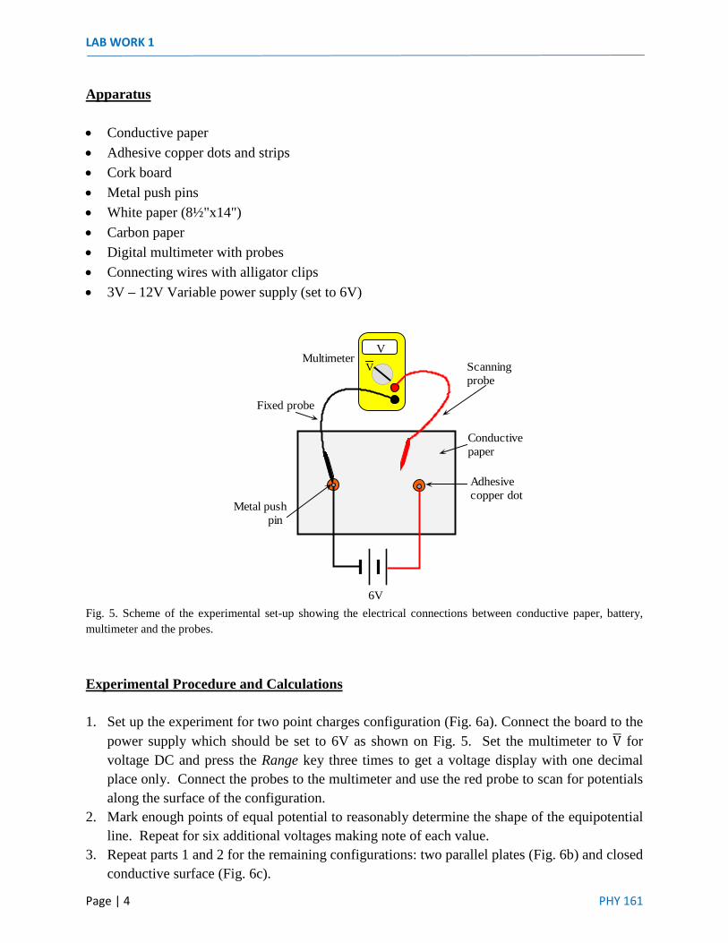
Fig. 5. Scheme of the experimental set-up showing the electrical connections between conductive paper, battery, multimeter and the probes.
Experimental Procedure and Calculations
1. Set up the experiment for two point charges configuration (Fig. 6a). Connect the board to the power supply which should be set to 6V as shown on Fig. 5. Set the multimeter to V for voltage DC and press the Range key three times to get a voltage display with one decimal place only. Connect the probes to the multimeter and use the red probe to scan for potentials along the surface of the configuration.
2. Mark enough points of equal potential to reasonably determine the shape of the equipotential line. Repeat for six additional voltages making note of each value.
3. Repeat parts 1 and 2 for the remaining configurations: two parallel plates (Fig. 6b) and closed conductive surface (Fig. 6c).
VScanningprobe
Conductivepaper
MultimeterV
Adhesivecopper dot
Metal push pin
Fixed probe
6V

EQUIPOTENTIAL AND ELECTRIC FIELD LINES
PHY 161 Page | 5
4. From the points you have marked, carefully construct the equipotential lines for each charge distribution.
5. Construct the electric field lines. Remember that electric field lines are always perpendicular to equipotential lines.
6. Calculate the electric field strength in 3 locations of your choice on each graph. 7. Estimate the amount of electric charge on the point electrodes (the configuration on Fig. 6a)
using the accumulated data.
Fig. 6. Configurations of charged metal electrodes on conductive paper: (a) two point charges, (b) two parallel plates, (c) closed conductive surface.
Questions
1. Is it possible for two different equipotential lines to cross each other? Explain why or why not?
2. Is it possible for two different electric field lines to cross each other? Explain why or why not?
3. Where do the electric field lines begin and end? If they are equally spaced at their beginning, are they equally spaced at the end? Along the way? Why?
4. If you wanted to push a charge along one of the electric field lines from one conductor to the other, how does the choice of electric field line affect the amount of work required? Explain.
5. The potential is everywhere the same on an equipotential line. Is the electric field everywhere the same on an electric field line? Explain.
6. How much work has to be done in order to move an electric charge along an equipotential line?
7. Where do the equipotential lines begin and end? Explain.
(a) (b) (c)

LAB WORK 1
Page | 6 PHY 161
PHY 161 Page | 7
LAB WORK 2
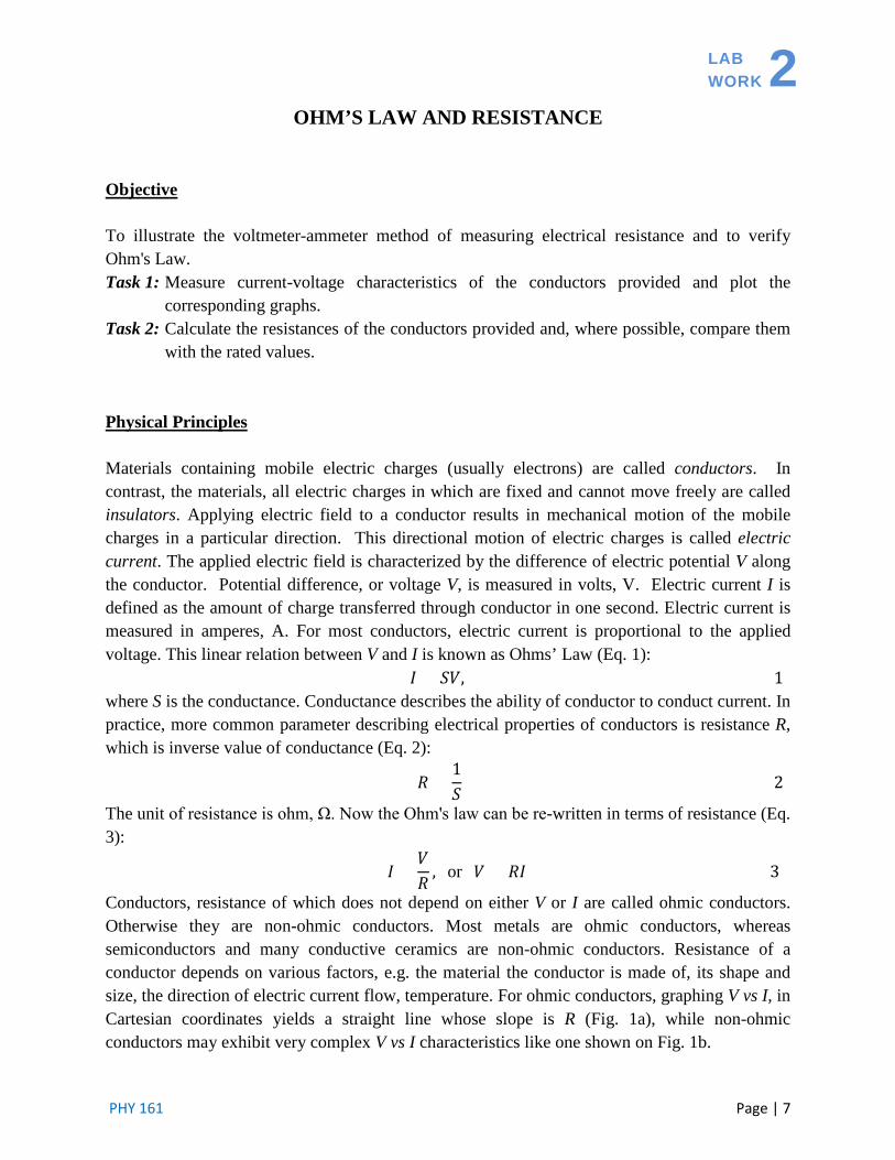
OHM’S LAW AND RESISTANCE Objective To illustrate the voltmeter-ammeter method of measuring electrical resistance and to verify Ohm's Law. Task 1: Measure current-voltage characteristics of the conductors provided and plot the
corresponding graphs. Task 2: Calculate the resistances of the conductors provided and, where possible, compare them
with the rated values. Physical Principles Materials containing mobile electric charges (usually electrons) are called conductors. In contrast, the materials, all electric charges in which are fixed and cannot move freely are called insulators. Applying electric field to a conductor results in mechanical motion of the mobile charges in a particular direction. This directional motion of electric charges is called electric current. The applied electric field is characterized by the difference of electric potential V along the conductor. Potential difference, or voltage V, is measured in volts, V. Electric current I is defined as the amount of charge transferred through conductor in one second. Electric current is measured in amperes, A. For most conductors, electric current is proportional to the applied voltage. This linear relation between V and I is known as Ohms’ Law (Eq. 1):
𝐼 = 𝑆𝑉, (1) where S is the conductance. Conductance describes the ability of conductor to conduct current. In practice, more common parameter describing electrical properties of conductors is resistance R, which is inverse value of conductance (Eq. 2):
𝑅 =1𝑆
(2)
The unit of resistance is ohm, Ω. Now the Ohm's law can be re-written in terms of resistance (Eq. 3):
𝐼 =𝑉𝑅
, or 𝑉 = 𝑅𝐼 (3)
Conductors, resistance of which does not depend on either V or I are called ohmic conductors. Otherwise they are non-ohmic conductors. Most metals are ohmic conductors, whereas semiconductors and many conductive ceramics are non-ohmic conductors. Resistance of a conductor depends on various factors, e.g. the material the conductor is made of, its shape and size, the direction of electric current flow, temperature. For ohmic conductors, graphing V vs I, in Cartesian coordinates yields a straight line whose slope is R (Fig. 1a), while non-ohmic conductors may exhibit very complex V vs I characteristics like one shown on Fig. 1b.

LAB WORK 2
Page | 8 PHY 161
(a) (b) Fig. 1. (a) Voltage applied to a conductor as a function of the induced current for an ohmic conductor. Slope of this dependence calculated as the change of voltage ∆V divided by the corresponding change of current ∆I equals resistance R of this conductor: R=∆V/∆I. (b) Non-ohmic conductors may exhibit complex non-linear dependences of voltage versus current. The ability of moving electrons to maneuver through a conducting material depends on the physical parameters of this material and on its temperature. Heating results in thermal agitation of moving electrons and atoms in the conductor. This agitation retards the directional motion of electrons and, consequently, increases resistance of the conductor. The current flow itself can increase temperature considerably: the greater the current in a conductor the higher its temperature. The actual dependence of resistance on temperature is a characteristic of the conducting material. It is measured by so-called temperature coefficient of resistivity α. This coefficient may be positive or negative and therefore the resistance of some conductors increases with temperature, whereas it decreases for the others. For instance, for tungsten α = +4.5×10⁻³ °C-1, for carbon (graphite) α = -5×10⁻⁴ °C-1. The change of resistance with temperature is given by the following formula (Eq. 4):
𝑅(𝑇) = 𝑅𝑅𝑇[1 + 𝛼(𝑇 − 𝑇𝑅𝑇)] (4) where R(T) is the resistance at temperature T; TRT is room temperature (usually 20°C) and RRT is the resistance at room temperature. Apparatus • Variable DC power supply • Ammeter (Digital Multimeter set to “mA” DC) • Voltmeter (Digital Multimeter set to “V” DC) • Tubular power rated resistor (100Ω) • Tungsten filament lamp (60W) • Carbon filament lamp (32cp) • Lamp socket
IVR slope∆∆
==
y=mxm=100.5+/-0.253
∆I
∆V

OHM’S LAW AND RESISTANCE
PHY 161 Page | 9
• Connecting wires • Knife switch with spades Procedure and Calculations 1. Set up the equipment as shown in Fig 2 with 100 Ω tubular resistor for R, a digital multimeter
(connect to the 400 mA input and set the dial to mA, press the yellow button to switch from AC to DC) for A, and a second digital multimeter for V (set the dial to V DC). Have your connections checked by your technician/instructor before turning on the power supply! Close the circuit and set the power supply Vo to 1, 2, 4, 6, 10, 14, 18, 22, 26 and 30V, recording V and I for each step.
Fig. 2. Circuit set-up used for the study of Ohm's Law by voltmeter-ammeter method. 2. Open the circuit and replace the tubular resistor with the tungsten filament lamp for R (Fig.
3). Have your connections checked by your technician/instructor before turning on the power supply! Close the circuit and set the power supply Vo to 1, 2, 4, 6, 10, 14, 18, 22, 26 and 30V, recording V and I for each step. When working with the lamp at low voltages allow the current to stabilize before recording it.
3. Open the circuit and remove the tungsten lamp and place the carbon filament lamp for R. Have your connections checked by your technician/instructor before turning on the power supply! Close the circuit and set the power supply Vo to 1, 2, 4, 6, 10, 14, 18, 22, 26 and 30V, recording V and I for each step. When working with the lamp at low voltages allow the current to stabilize before recording it.
Switch
V A 400mA
Power supply
Voltmeter
Ammeter
Resistor
V
A
R
+ -
+ - A DC
mA
V DC
V

LAB WORK 2
Page | 10 PHY 161
Fig. 3. Circuit with tungsten filament lamp in place for R. 4. Plot the calculated data for each resistor on a graph using V as the y-axis and I as the x-axis
(3 curves in one graph). See Fig. 4 for sample graph.
Fig. 4. Sample graph of V vs I for tubular resistor, tungsten bulb and carbon bulb.
5. On the graph, fit the experimental points for the tubular resistor with a straight line. Find the slope of this line. Compare the found value with the rated resistance 100 ohm.
6. Calculate resistance of 100 ohm resistor using your data for each voltage step. Find average value of the resistance and the experimental error. Compare the calculated value with that obtained from the graph.
7. Using the data obtained in the Procedures 1, 2 and 3 compute R for each pair of V and I. Plot R as a function of I for both lamps. See Fig. 5 for sample graph.
KnifeSwitch
Power Supply
Multimeterset to V DC
Multimeterset to mA DC
TungstenLamp
400mAInput
When the switch lever is down as above, the circuit is closedand current is allowed to flow through the circuit.Current I through the circuit as well as voltage V across theresistor can be recorded.

OHM’S LAW AND RESISTANCE
PHY 161 Page | 11
Fig. 5. Sample data of R vs I for tubular resistor, tungsten bulb and carbon bulb.
Questions 1. Of the three objects you measured in this experiment (tubular resistor and two lamps), which
are ohmic resistors and which are not? Explain. 2. What is your explanation for the fact that the current induced in the lamps does not follow
Ohm’s Law? 3. What do the plots tell you about the temperature coefficient of resistivity of each object
used? 4. Using formula (4) estimate the maximum temperature the filaments in the lamps reach during
the measurements. 5. Predict the current, which would be induced in the resistors you measured if a voltage of 40
V could be applied.

LAB WORK 2
Page | 12 PHY 161
PHY 161 Page | 13
LAB WORK 3
RESISTIVITY
Objective
Objective of this lab work is to measure resistivity of a conductor with uniform cross-section over its length. Task 1: Determine the resistance of a piece of wire using the voltmeter-ammeter method. Task 2: Determine dependence of the resistance of a piece of wire as a function of its length. Task 3: Calculate the resistivity of the material the wire resistance is made of.
Physical Principles
When voltage is applied between the ends of a conductor an electric current flows through this conductor. The current strength I depends on the magnitude of voltage V and on many other physical parameters of the conductor itself and its surroundings. These parameters determine the resistance R of the conductor. Experimentally, the value R can be measured as a ratio of voltage over current (Eq. 1):
𝑅 =𝑉𝐼
(1)
At a constant temperature, resistance of most conductors primarily depends on their shape and size as well as on the properties of the material this conductor is made of. For a conductor of length L and uniform cross-section of area A, R can be found as (Eq. 2):
𝑅 = 𝜌𝐿𝐴
, (2)
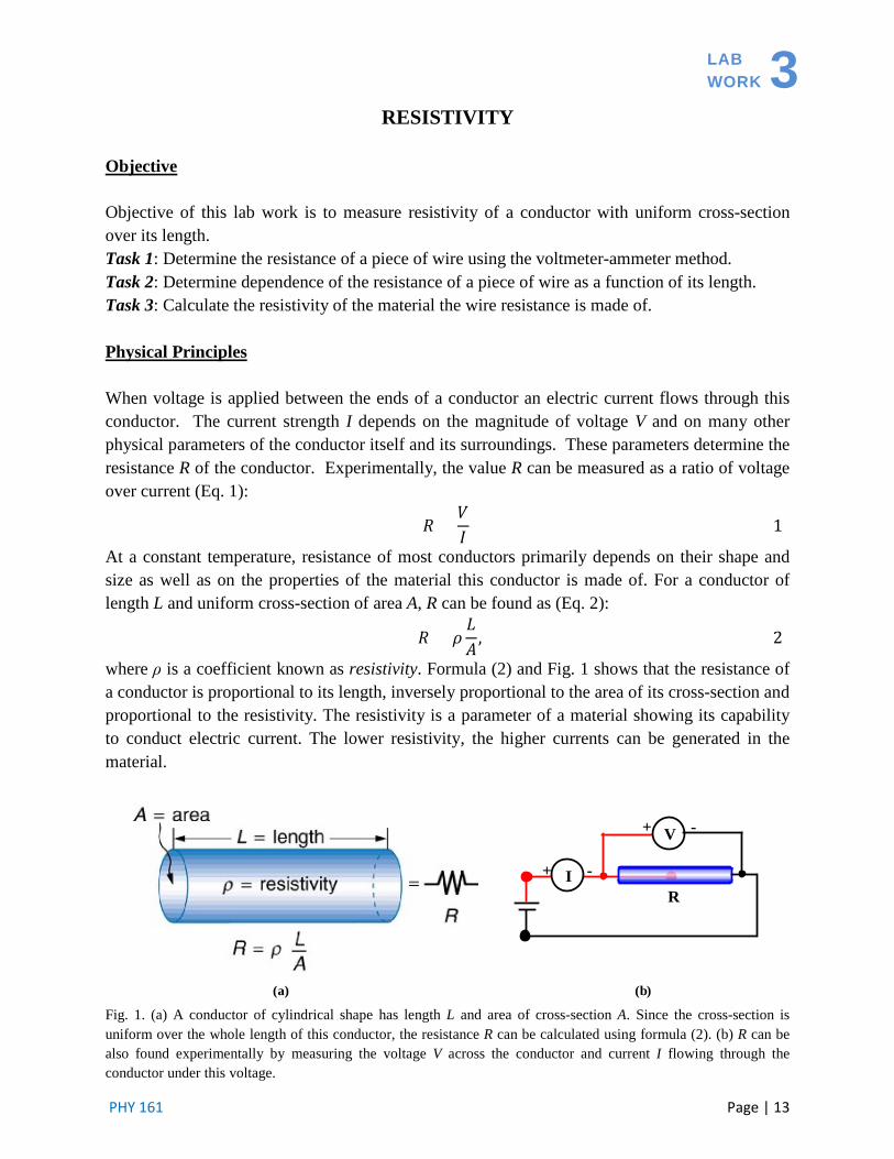
where ρ is a coefficient known as resistivity. Formula (2) and Fig. 1 shows that the resistance of a conductor is proportional to its length, inversely proportional to the area of its cross-section and proportional to the resistivity. The resistivity is a parameter of a material showing its capability to conduct electric current. The lower resistivity, the higher currents can be generated in the material.
Fig. 1. (a) A conductor of cylindrical shape has length L and area of cross-section A. Since the cross-section is uniform over the whole length of this conductor, the resistance R can be calculated using formula (2). (b) R can be also found experimentally by measuring the voltage V across the conductor and current I flowing through the conductor under this voltage.
I
V
+ -
+ -
R
(a) (b)

LAB WORK 3
Page | 14 PHY 161
Experimentally, the resistivity of a conductor can be found by measuring its resistance and its dimensions. If a piece of wire of length L and diameter D is used as the conductor (Fig. 1), its resistivity can be calculated using formula (Eq. 3):
𝜌 =𝑅𝜋𝐷2
4𝐿. (3)
When the voltmeter-ammeter method is used to measure resistance: R = V/I (see manual of the lab work “Ohm’s Law and Resistance”), then the final formula for the calculation of resistivity is as shown below (Eq. 4):
𝜌 =𝑉𝜋𝐷2
𝐼4𝐿, (4)
where V is the voltage applied to the wire and I is the current flowing through the wire under this voltage. In order to better understand the relationship between the parameters in the formulas above, try the interactive applet: http://phet.colorado.edu/sims/resistance-in-a-wire/resistance-in-a-wire_en.html
Apparatus
• Variable DC power supply • Wire resistor (R) of diameter D = 0.64 mm • Digital multimeter (V) • Digital multimeter (A) • 500 Ω tubular ballast resistor (Ro) • Connecting wires
Procedure and Calculations:
Part I: 1. Set up the equipment shown in Fig 2: Power supply for Vo, the 500 Ω tubular resistor for the
ballast resistor Ro, digital voltmeter for V, digital ammeter for I, the wire resistor for R. Have your connections checked by your instructor/technician before turning on the power supply!
2. Set the voltmeter to mV and place its leads (red/black connectors) at the 0cm and the 100cm posts (as shown on Figs 2a and 2b.) Varying voltage on the power supply in 1 V steps take the reading from the ammeter I and the voltmeter V for each voltage step.

RESISTIVITY
PHY 161 Page | 15
RIVSlope =∆∆
=
∆V
∆I
Fig. 2a. Schematic of circuit set-up for the measurement of resistance using voltmeter-ammeter method.
Fig. 2b. Experimental set-up used for Part I.
3. Plot the recorded data using voltage V as ordinate and current I as abscissa (see Fig. 3 for
sample graph). Fit the experimental points with a straight line passing through the origin. Determine the slope of this line ∆V/∆I. The obtained value is the total resistance R of the wire: R = ∆V/∆I.
Fig. 3. Voltage across the wire as a function of current passing through it (current-voltage characteristic of the wire). Slope of this dependence equals resistance of the wire.
Ro
Power Supply
R100cm0cm
- +
+ -V A
A DC
mA
400mA
Vo+
+-
- V DC
mV
Switch
Multimeter tomeasure voltage
Multimeter tomeasure current

LAB WORK 3
Page | 16 PHY 161
4. Use formula (3) and resistance R found from the V vs I graph to calculate the resistivity of the wire.
Part II: 1. With the circuit set-up as on Fig. 4 set the voltage on the power supply, Vo to 10 V. Record
the current I, which will remain constant thereafter. By means of the movable connector (red connector from the voltmeter) measure voltage V for different lengths L of the wire by tapping the wire at points from 1 cm to 100 cm in 10 cm steps (Fig. 4).
Fig. 4. (a) Scheme of the set-up used for the measurements of resistivity when varying the length of the conductor
Fig. 4. (b) Experimental set-up to obtain resistivity of the conductor.
2. Based on the recorded data, compute R in ohms, for each length L. Plot R as a function of L
(R as ordinate and L as abscissa, Fig. 5). Fit the experimental points with a straight line passing through the origin. Calculate slope ∆R/∆L of this line.
Ro
Power Supply
R100cm0cm
- +
+ -V A
A DC
mA
400mA
Vo+
+-
- V DC
mV
Switch
Multimeter tomeasure voltage
Multimeter tomeasure current
RESISTIVITY
PHY 161 Page | 17
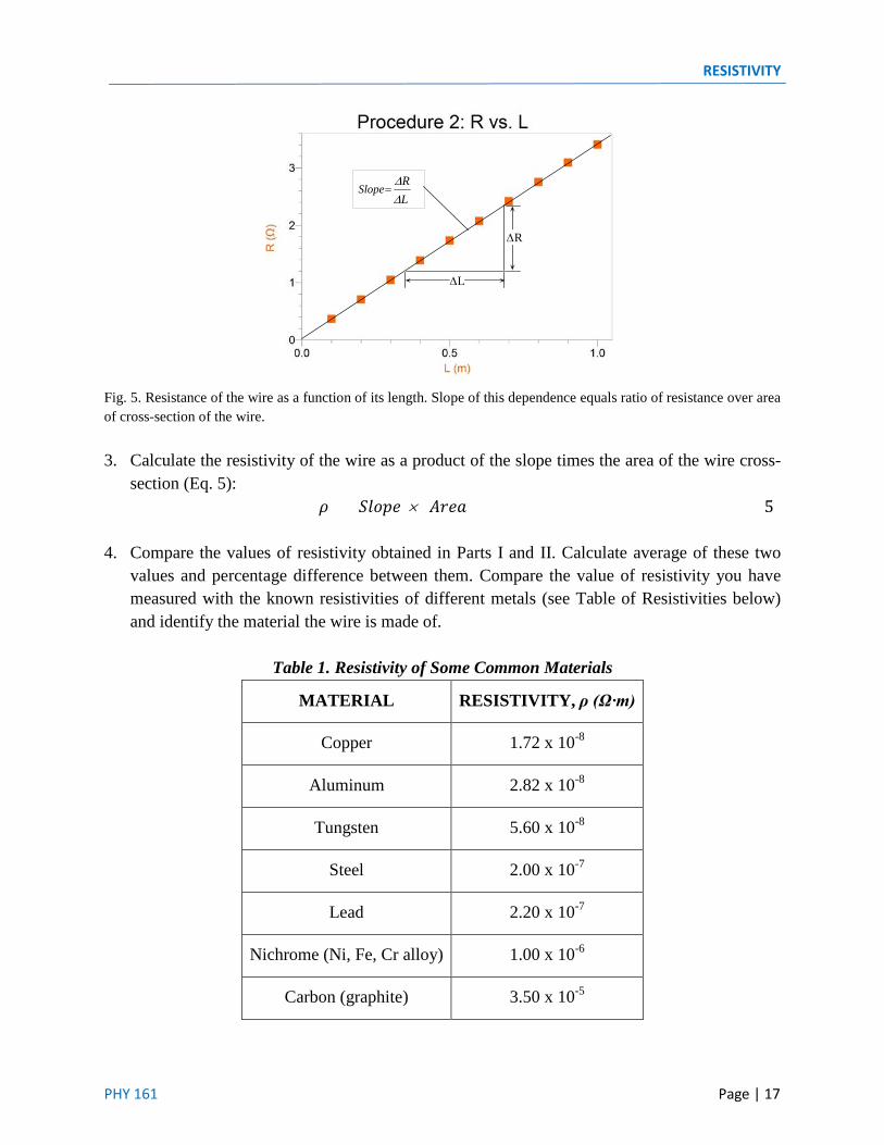
Fig. 5. Resistance of the wire as a function of its length. Slope of this dependence equals ratio of resistance over area of cross-section of the wire. 3. Calculate the resistivity of the wire as a product of the slope times the area of the wire cross-
section (Eq. 5): 𝜌 = (𝑆𝑙𝑜𝑝𝑒)× (𝐴𝑟𝑒𝑎) (5)
4. Compare the values of resistivity obtained in Parts I and II. Calculate average of these two
values and percentage difference between them. Compare the value of resistivity you have measured with the known resistivities of different metals (see Table of Resistivities below) and identify the material the wire is made of.
Table 1. Resistivity of Some Common Materials
MATERIAL RESISTIVITY, ρ (Ω·m)
Copper 1.72 x 10⁻⁸
Aluminum 2.82 x 10⁻⁸
Tungsten 5.60 x 10⁻⁸
Steel 2.00 x 10⁻⁷
Lead 2.20 x 10⁻⁷
Nichrome (Ni, Fe, Cr alloy) 1.00 x 10⁻⁶
Carbon (graphite) 3.50 x 10⁻⁵
∆R
∆L
RIVSlope =∆∆
=∆R∆L

LAB WORK 3
Page | 18 PHY 161
Questions
1. What role does the ballast resistor R0 play in the circuit used this lab work? 2. Based on the value of resistivity you calculated, what is the material the wire resistor is made
of? 3. Is the wire resistor an ohmic conductor? Support your answer with the experimental data you
obtained. 4. Do resistance and resistivity depend on:
- the wire length? - the wire cross-section? - the wire shape?

PHY 161 Page | 19
LAB WORK 4
RESISTORS AND CAPACITORS CONNECTED IN SERIES AND IN PARALLEL
Objective
Task 1: To measure total resistance of resistors connected in series and in parallel and compare the measured values with the calculated ones.
Task 2: To measure total capacitance of capacitors connected in series and in parallel and compare the measured values with the calculated ones.
Physical Principles
It is known that the total resistance RT of n resistors connected in series (Fig. 1a) equals sum of their resistances (Eq. 1):
𝑅𝑇 = 𝑅1 + 𝑅2 + 𝑅3 + ⋯+ 𝑅𝑛 (1)
Fig. 1. (a) Circuit of resistors connected series. (b) Circuit of resistors connected in parallel. If the resistors are connected in parallel (Fig. 1b), their total resistance RT can be found using the following formula (Eq. 2):
1𝑅𝑇
=1𝑅1
+1𝑅2
+1𝑅3
+ ⋯+1𝑅𝑛
(2)
Total capacitance CT of n capacitors connected in series (Fig. 2a) and in parallel (Fig. 2b) can be found in a similar way. However, the formulae (1) and (2) must be swapped. That is, the total capacitance of capacitors connected in series is given by the formula (Eq. 3):
1𝐶𝑇
=1𝐶1
+1𝐶2
+1𝐶3
+ ⋯+1𝐶𝑛
, (3)
whereas the total capacitance CT of capacitors connected in parallel is just a sum of the involved capacitances (Eq. 4):
𝐶𝑇 = 𝐶1 + 𝐶2 + 𝐶3 + ⋯+ 𝐶𝑛 (4)
R1
R2
Rn
R1 R2 Rn.....
(a) (b)

LAB WORK 4
Page | 20 PHY 161
Fig. 2. (a) Circuit of capacitors connected in series. (b) Circuit of capacitors connected in parallel. Real circuits of resistors and capacitors may have various combinations of series and parallel connections. The simplest combinations can be explored using only three resistors, or three capacitors. The formula for total resistance of three resistors in series (Fig. 3a) is simplified to (Eq. 5):
𝑅𝑇 = 𝑅1 + 𝑅2 + 𝑅3 (5) and for three resistors in parallel (Fig. 3b) we have (Eq. 6):
𝑅𝑇 =𝑅1𝑅2𝑅3
𝑅1𝑅2 + 𝑅2𝑅3 + 𝑅1𝑅3 (6)
Fig. 3. (a) Circuit of three resistors connected series. (b) Circuit of three resistors connected in parallel. The circuits can combine series and parallel connections (Fig. 4a and Fig. 4b). The total resistance of the circuit in Fig. 4a is (Eq. 7):
𝑅𝑇 =(𝑅1+𝑅2)𝑅3𝑅1 + 𝑅2 + 𝑅3
, (7)
while the total resistance of the circuit in Fig. 4b can be found as (Eq. 8):
𝑅𝑇 =𝑅1𝑅2𝑅1 + 𝑅2
+ 𝑅3 (8)
C1
C2
Cn
C1 C2 Cn.....
(a) (b)
R1
R2
R3
R1 R2 R3
(a) (b)
CONNECTION OF RESISTORS AND CAPACITORS IN SERIES AND PARALLEL
PHY 161 Page | 21
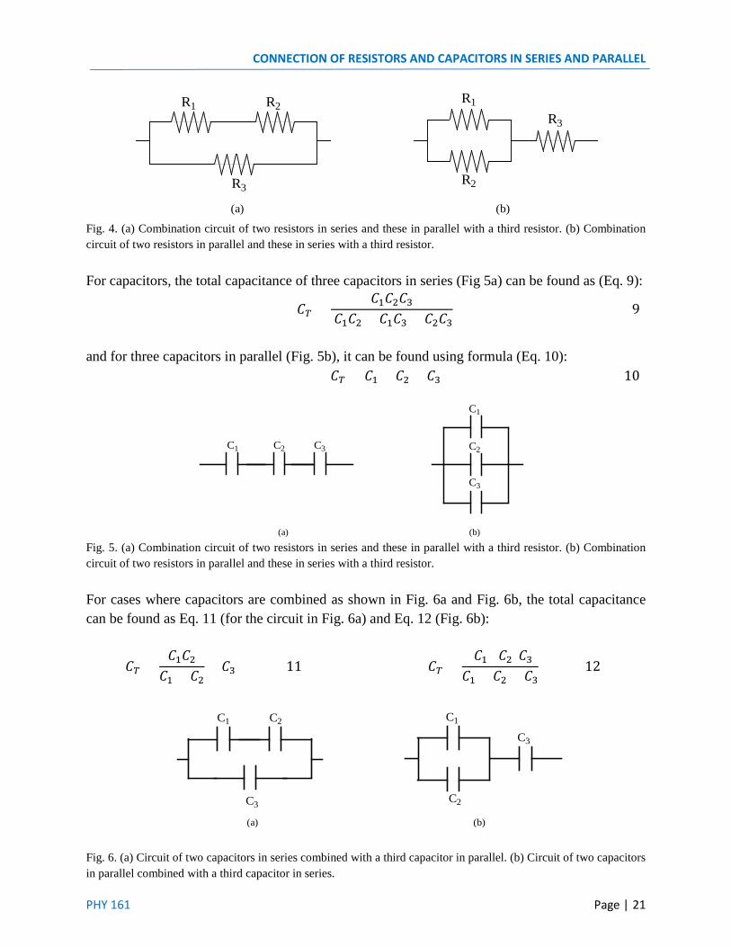
Fig. 4. (a) Combination circuit of two resistors in series and these in parallel with a third resistor. (b) Combination circuit of two resistors in parallel and these in series with a third resistor. For capacitors, the total capacitance of three capacitors in series (Fig 5a) can be found as (Eq. 9):
𝐶𝑇 =𝐶1𝐶2𝐶3
𝐶1𝐶2 + 𝐶1𝐶3 + 𝐶2𝐶3 (9)
and for three capacitors in parallel (Fig. 5b), it can be found using formula (Eq. 10):
𝐶𝑇 = 𝐶1 + 𝐶2 + 𝐶3 (10)
Fig. 5. (a) Combination circuit of two resistors in series and these in parallel with a third resistor. (b) Combination circuit of two resistors in parallel and these in series with a third resistor. For cases where capacitors are combined as shown in Fig. 6a and Fig. 6b, the total capacitance can be found as Eq. 11 (for the circuit in Fig. 6a) and Eq. 12 (Fig. 6b):
𝐶𝑇 =𝐶1𝐶2𝐶1 + 𝐶2
+ 𝐶3 (11) 𝐶𝑇 =(𝐶1+𝐶2)𝐶3𝐶1 + 𝐶2 + 𝐶3
(12)
Fig. 6. (a) Circuit of two capacitors in series combined with a third capacitor in parallel. (b) Circuit of two capacitors in parallel combined with a third capacitor in series.
R1
R2
R3
R1 R2
R3
(a) (b)
C1
C2
C3
C1 C2 C3
(a) (b)
(a) (b)
C1 C2
C3
C1
C3
C2

LAB WORK 4
Page | 22 PHY 161
Apparatus
• 3.3 kΩ, 1 kΩ and 5.1 kΩ resistors • 47 μF, 20 μF and 10 μF axial capacitors • Snap-circuit connectors • Snap-circuit board • Multimeter (with capacitance feature)
Procedure 1. Resistors in Series and in Parallel
1. Measure the actual resistance (Ω-setting on the multimeter) of each resistor. 2. Measure the total resistance for the following series combinations (Fig. 7):
R1 and R2 R1 and R3 R2 and R3 R1, R2 and R3
Fig. 7. Example of three resistors connected in series.
3. Measure the total resistance for the following parallel combinations (Fig. 8):
R1 and R2 R1 and R3 R2 and R3 R1, R2 and R3
Fig. 8. Example of three resistors connected in parallel.
4. Measure the total resistance for the following mixed combinations shown in Fig. 9:
R1 and R2 in series and this combination in parallel with R3 R1 and R2 in parallel and this combination in series with R3 Any other combinations you can come up with (extra points!).

CONNECTION OF RESISTORS AND CAPACITORS IN SERIES AND PARALLEL
PHY 161 Page | 23
(a) (b)
Fig. 9. (a) Two resistors in series and this combination in parallel with a third resistor. (b) Two resistors in parallel and this combination in series with a third resistor.
Procedure 2. Capacitors in Series and in Parallel
1. Measure the actual capacitance (Ω-setting on the multimeter, press yellow button for μF reading) of each capacitor.
2. Measure the total capacitance for the following series combinations (Fig. 10): C1 and C2 C1 and C3 C2 and C3 C1, C2 and C3
Fig. 10. Example of three capacitors connected in series.
3. Measure the total capacitance for the following parallel combinations (Fig. 11):
C1 and C2 C1 and C3 C2 and C3 C1, C2 and C3
Fig. 11. Example of three capacitors connected in parallel. 4. Measure the total capacitance for the following mixed combinations shown in Fig. 12:
C1 and C2 in series and this combination in parallel with C3 C1 and C2 in parallel and this combination in series with C3 Any other combinations you can come up with (extra points!).

LAB WORK 4
Page | 24 PHY 161
(a) (b) Fig. 12. (a) Two capacitors in series and this combination in parallel with a third capacitor. (b) Two capacitors in parallel and this combination in series with a third capacitor.
Calculations
1. Calculate the total resistances for all combinations of resistors using the corresponding formulae. Compare the result with the measured values.
2. Repeat these calculations for assemblies of capacitors and compare the calculated values with the experimental ones.
3. Calculate the experimental error (percent difference between the measured and calculated values).
Questions
1. Suppose you are given several resistors whose resistances are within the range 15 to 40 Ω. You connect them all in series and let your three partners measure the total resistance. Three different measurements have been obtained: 8, 34 and 92 Ω. Which of these three you would assume to be correct?
2. Suppose you are given several resistors whose resistances are within the range 15 to 40 Ω. You connect them all in parallel and let your three partners measure the total resistance. Three different measurements have been obtained: 8, 34 and 92Ω. Which of these three you would assume to be correct?
3. Suppose you are given several capacitors whose capacitances are within the range 12 to 50 nF. You connect all the capacitors in series and let your three partners measure the total capacitance. Three different measurements have been obtained: 8, 44 and 102 nF. Which of these three you would assume to be correct?
4. Suppose you are given several capacitors whose capacitances are within the range 12 to 40 nF. You connect all the capacitors in parallel and let your three partners measure the total capacitance. Three different measurements have been obtained: 8, 44 and 102 nF. Which of these three you would assume to be correct?
5. A circuit of resistors connected in series is plugged in a 120 V outlet. What can you tell about the voltage on each of resistor and current in each resistor?
6. A circuit of capacitors connected in parallel is plugged in a 120 V outlet. What can you tell about the voltage on each capacitor and current in each capacitor?

PHY 161 Page | 25
LAB
WORK 5
DIRECT CURRENT METERS
Objective
To learn the principles of operation of analog electromagnetic DC voltmeter and ammeter and
the principles of measurement of DC voltage and DC current using these devices.
Task 1: Design, assemble and calibrate a rudimentary analog ammeter.
Task 2: Design, assemble and calibrate a rudimentary analog voltmeter.
Task 3: Perform measurements of current and voltage with assembled DC meters.
Physical Principles
The devices used for the measurements of electric current and voltage in direct current (DC)
circuits are known as DC ammeters and DC voltmeters (DC meters). Two basic components of a
rudimentary analog electromagnetic DC meter are DC galvanometer and resistor (shunt)
connected to the galvanometer in a specified way.
A galvanometer is a tiny electromagnet (coil of wire), which can move in magnetic field when
current passes through it. A pointer fixed to the electromagnet shows this motion. A
galvanometer is constructed so that the deflection of the pointer is proportional to the current
flowing through the galvanometer coil. Two main parameters of a galvanometer are its electrical
resistance (internal resistance) RG and the current required for full scale deflection of the pointer
(current of galvanometer) IG. Galvanometers are very delicate and sensitive devices, which
cannot stand high currents and voltages. Therefore, they can be used as ammeters and voltmeters
directly only for the measurements of small currents (usually below 1 mA) and small voltages
(usually below 0.1 V). In order to use a galvanometer as an ammeter for high currents, or a
voltmeter for high voltages, it must be connected to a shunt of resistance RS. The shunt restricts
current flowing through the galvanometer and prevents it from destruction.
In order to convert a galvanometer into an ammeter, a shunt is connected in parallel to the
galvanometer (Fig. 1).
Fig. 1. Electric circuit of an ammeter composed of a galvanometer and a shunt. A shunt is connected to the
galvanometer in parallel. The distribution of electric current flowing through the ammeter is shown with arrows.
Rs ammeterIs
IGAmmeter
IG

LAB WORK 5
Page | 26 PHY 161
The measured (total) current I is split inside the ammeter into two currents: IG (small portion)
flowing through the galvanometer and the other IS ammeter (main stream) flowing through the shunt
(Eq. 1):
I = IG + IS ammeter (1)
The resistance of the shunt of an ammeter RS ammeter , which is required to convert a galvanometer
to the ammeter can be found as following (Eq. 2):
𝑹𝑺 𝒂𝒎𝒎𝒆𝒕𝒆𝒓 =𝑹𝑮𝑰𝑮
𝑰𝒎−𝑰𝑮 (2)
where Im is the maximum current to be measured by the ammeter. It is seen that the greater the
maximum current Im the smaller the resistance of the shunt. Usually, the resistance of shunts used
in electromagnetic ammeters amounts to a fraction of an ohm.
In order to convert a galvanometer into a voltmeter, the shunt is connected in series to the
galvanometer (Fig. 2). In this case, the current flowing through the voltmeter passes both shunt
and galvanometer. However, the voltage measured by the voltmeter V is split into two parts (Eq.
3): the voltage across the galvanometer VG (small part) and the voltage across the shunt VS voltmeter
(a great part). Thus:
V = VG + VS voltmeter (3)
Fig. 2. Electric circuit of a voltmeter composed of galvanometer and shunt. The current flowing through the
voltmeter is the current of galvanometer IG.
The resistance of the shunt RS voltmeter, which is required to convert a galvanometer to a voltmeter
can be found using formula (Eq. 4).
𝑹𝑺 𝒗𝒐𝒍𝒕𝒎𝒆𝒕𝒆𝒓 =𝑽𝒎
𝑰𝑮− 𝑹𝑮 (4)
where Vm is the maximum voltage to be measured by the voltmeter.
Apparatus
Power supply
Two digital multimeters (V and A)
One short red and one short black connecting wires
G
Rs voltmeter
IG Voltmeter

DIRECT CURRENT METERS
PHY 161 Page | 27
Two small snap-circuit boards
+/-500 µA galvanometer
Snap-circuit resistors: 10 kΩ, 1 kΩ, 100 Ω and 510 Ω
Two snap-circuit SPST switches
Snap-circuit connectors: 1-point x 1, 2-point x 4, 3-point x 3, 6-point x 1, 7-point x 1
Snap-circuit to banana plug connectors (3 red, 3 black)
Decade resistance box (0.1 Ω resolution)
Preliminary set-up
Use the snap-circuit elements to assemble the circuit boards as shown below:
Fig. 3. (a) Circuit Board 1 for determining RG and testing designed 5 mA analog ammeter. (b) Circuit Board 2 for
testing designed 5 V analog voltmeter.
Procedure and Calculations
Part I. Determining the internal resistance of the galvanometer
1. Connect the power supply to the supplied circuit board containing an SPST switch, a 10kΩ
resistor, a +/-500 µA galvanometer G, and a multimeter V as shown on Fig. 4.
Fig. 4. Initial circuit of the set-up used for the measurement of the internal resistance RG of galvanometer.
V
V
10 k
V A
OFF
+/-500A
G
10 k
1 k100
510
(a) (b)
Circuit Board 1 Circuit Board 2
OFFOFF

LAB WORK 5
Page | 28 PHY 161
2. Set the multimeter to V DC. Turn on the power supply. Set the switch to ON (close the
circuit) to allow current to flow through the circuit. Slowly increase voltage on the power
supply so that the galvanometer reaches full scale. Record the voltage as read from the
multimeter, this represents VG. Be careful when increasing the voltage; do it gradually to
avoid overloading the galvanometer! Set the switch to OFF. Turn off the multimeter and
remove from circuit.
3. Determine the internal resistance of the galvanometer RG using the formula: RG = VG/IG.
Part II. Converting the galvanometer to 5 mA ammeter
1. Determine the shunt resistance RS ammeter required to convert the galvanometer (IG = 500 ×
10−6A) to a 5 mA ammeter (Im = 5 × 10⁻³A). Use Eq. 2 as follows:
𝑅𝑆 𝐴𝑚𝑚𝑒𝑡𝑒𝑟 = 𝑅𝐺𝐼𝐺
𝐼𝑚−𝐼𝐺=
𝑉𝐺
5 × 10⁻³ − 500 × 10−6
2. Set the calculated RS ammeter value on the decade resistor box and connect it in parallel to the
galvanometer (Fig. 5). This combination is now your new analog 5mA Ammeter.
Fig. 5. Electric circuit of the developed ammeter.
3. Verify that the designed Ammeter is in fact a 5 mA range ammeter. On the circuit board that
was used for part I, swap the 10 kΩ resistor with a 1 kΩ resistor. Connect your new
Ammeter as shown on Fig. 6. Remove the 3pt-snap connector to create a gap where the
digital ammeter (labeled A) will be inserted. Make sure to connect the positive lead into the
400 mA input of the multimeter! Set multimeter to mA DC.
Fig. 6. Circuit set-up for the verification of the designed Ammeter.
4. Close the circuit and slowly increase the voltage on the power supply to obtain maximum
deflection on the designed Ammeter. Note, that the full scale of the Ammeter is supposed to
be 5 mA. Compare the reading of the new Ammeter with that of the digital ammeter.
New Ammeter
+/-500A
G
RS
1 k
V A
OFF
A
mA
400mA
+/-500A
G
RSNew Ammeter

DIRECT CURRENT METERS
PHY 161 Page | 29
5. Vary the voltage on the power supply and record three different readings of current on the
designed Ammeter and compare them with the readings of the digital ammeter.
6. Lower the voltage on the power supply to about 4 V. Open the circuit, turn off the
multimeter. Disconnect the galvanometer and the decade box from the circuit. Carefully
remove the circuit board and set aside.
Part III. Converting the galvanometer to a 5 V voltmeter
1. Use the resistance of the galvanometer RG to determine the shunt resistance RS voltmeter
required to design a 5 V voltmeter. Use Eq. 4 as follows:
𝑅𝑆 𝑣𝑜𝑙𝑡𝑚𝑒𝑡𝑒𝑟 =𝑉𝑚
𝐼𝐺− 𝑅𝐺 =
5
500 × 10−6− 𝑅𝐺
2. Set the decade box to the calculated shunt RS voltmeter and connect it in series to the
galvanometer (Fig. 7). This combination is your designed Voltmeter. The maximum reading
of the galvanometer now corresponds to voltage 5 V.
Fig. 7. Electric circuit of the designed Voltmeter.
3. Connect the digital multimeter (V) in parallel to your New Voltmeter.
4. Connect the second circuit board to the power supply. Connect the new voltmeter and digital
voltmeter to the circuit as shown on Fig 8. Set the digital voltmeter to V DC.
V A
OFF
V
V
100
510
New Voltmeter
+/-500A
Rs
G
Fig. 8. New Voltmeter is set in the circuit ready for verification with a digital multimeter.
New Voltmeter
Rs
G
LAB WORK 5
Page | 30 PHY 161
5. Set switch to ON. Slowly increase the voltage to obtain 5 V as per the new design (note that
500 reading on the galvanometer scale now corresponds to 5 V). Check the actually supplied
voltage with the digital voltmeter.
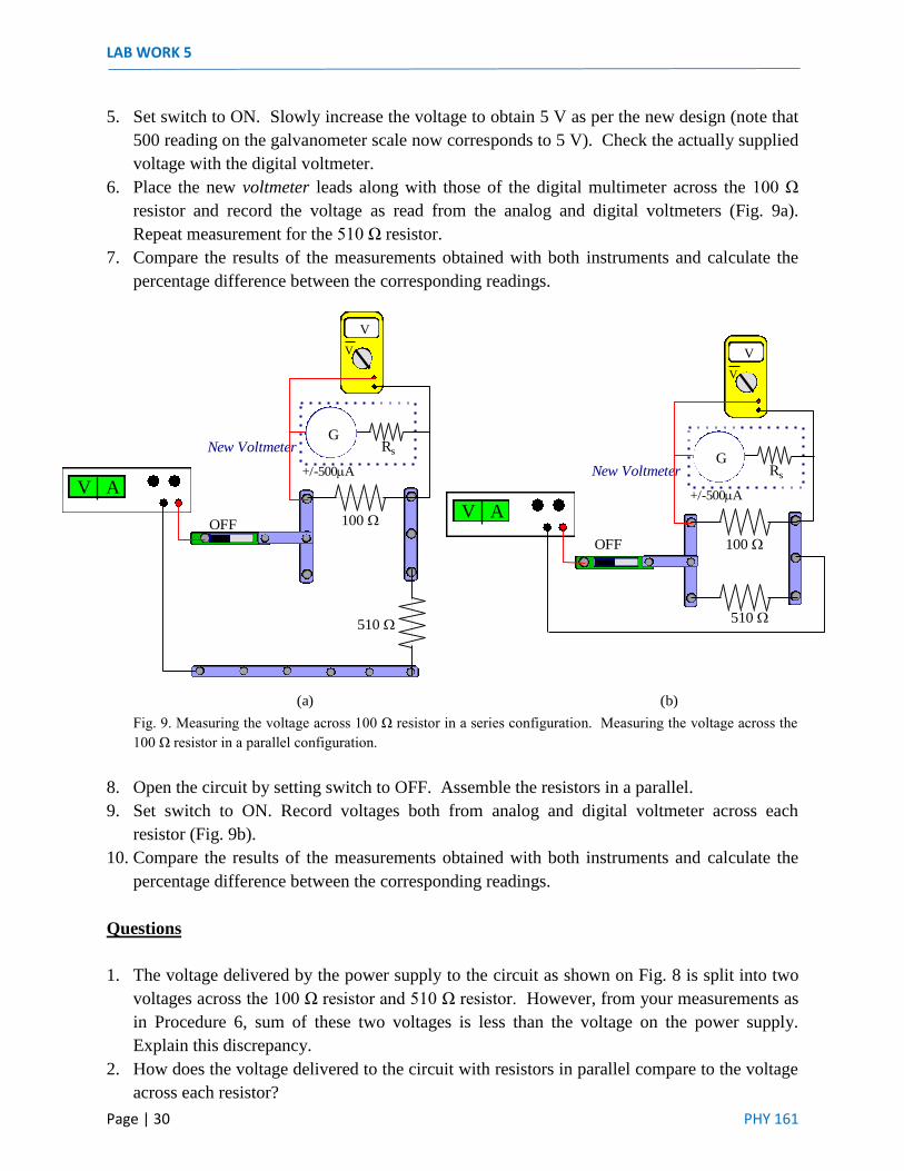
6. Place the new voltmeter leads along with those of the digital multimeter across the 100 Ω
resistor and record the voltage as read from the analog and digital voltmeters (Fig. 9a).
Repeat measurement for the 510 Ω resistor.
7. Compare the results of the measurements obtained with both instruments and calculate the
percentage difference between the corresponding readings.
Fig. 9. Measuring the voltage across 100 Ω resistor in a series configuration. Measuring the voltage across the
100 Ω resistor in a parallel configuration.
8. Open the circuit by setting switch to OFF. Assemble the resistors in a parallel.
9. Set switch to ON. Record voltages both from analog and digital voltmeter across each
resistor (Fig. 9b).
10. Compare the results of the measurements obtained with both instruments and calculate the
percentage difference between the corresponding readings.
Questions
1. The voltage delivered by the power supply to the circuit as shown on Fig. 8 is split into two
voltages across the 100 Ω resistor and 510 Ω resistor. However, from your measurements as
in Procedure 6, sum of these two voltages is less than the voltage on the power supply.
Explain this discrepancy.
2. How does the voltage delivered to the circuit with resistors in parallel compare to the voltage
across each resistor?
V A
OFF
V
V
100
510
New Voltmeter
V A
OFF
V
V
100
510
New Voltmeter
(a) (b)
+/-500A
Rs
+/-500A
Rs
G
G

DIRECT CURRENT METERS
PHY 161 Page | 31
3. Calculate the internal resistance of your new Ammeter.
4. Calculate the internal resistance of your new Voltmeter.
5. Which measurements are more accurate, performed with the new Ammeter and new
Voltmeter, or with the digital multimeters? Explain your answer.
6. Given a galvanometer with a full scale deflection of 200 μA and an internal resistance of 100
Ω:
5a. calculate the value of shunts and draw a circuit showing the conversion of this
galvanometer to a multi-range ammeter with full scale deflections of 0.1, 1, and 10 A.
5b. calculate the value of shunts and draw a circuit showing the conversion of this
galvanometer to a multi-range voltmeter with full scale deflections of 10, 100 and 1000 V.

LAB WORK 5
Page | 32 PHY 161

PHY 161 Page | 33
LAB WORK 6
KIRCHHOFF'S RULES Objective Experimental verification of Kirchhoff's rules by measuring voltages and currents in a DC circuit and comparing them with those calculated with Kirchhoff's rules. Task 1: Measurement of currents in two junctions of a given circuit and calculation of their
algebraic sum. Task 2: Measurement of voltages across resistors and batteries constituting three closed loops in
a given circuit and calculation of their algebraic sum. Physical Principles Kirchhoff's rules are known as a method of calculation of currents and voltages in DC circuits. Any DC circuit consists of sources of electromotive force, resistors, connecting wires and
junctions. Fig. 1 shows a simple DC circuit composed of two batteries of electromotive forces ε1
and ε2 and three resistors of resistances R1, R2, and R3.
Fig. 1. Schematic of a simple DC circuit The First Kirchhoff's Rule states: At any junction, the sum of all currents entering the junction equals the sum of all currents leaving the junction. In other words, the algebraic sum of all currents at any junction equals zero. It is important to note that in this sum the currents entering the junction are taken as positive, while the ones leaving the junction are taken as negative. A way to simplify this rule is to state that the sum of the currents entering the junction equals to the sum of the currents exiting the junction. The Second Kirchhoff's Rule states: The sum of the voltages around any closed loop equals zero. Each term must be taken with the corresponding sign (positive, or negative). This sign can be found taking into account the direction of the passing loop and the direction of current flow (Fig. 2). The voltage on a resistor is positive (+RI) if these two directions at this resistor are opposite. If at a resistor both directions coincide, the voltage on it is negative (-RI). For batteries, the rule of sign says: when a battery is passed from positive terminal to negative terminal, its
R1
R2
R3
ε1
ε2
b
c
+ -
+ -
a
d
f

LAB WORK 6
Page | 34 PHY 161
electromotive force is taken as negative (-Ɛ). Otherwise it is taken as positive (+Ɛ). This rule of signs is shown in Table 1 below.
Table 1. Sign Conventions for voltages on batteries and resistors in DC circuits. Blue arrows show the path direction around the loop; red arrows show direction of the current flow. Fig. 2 depicts sample results after applying both rules to the circuit of Fig. 1. For example, the junction rule is applied at node b and the loop rule is applied to loop abdf:
Fig. 2. – Sample Application of Kirchhoff’s First and Second Rules
ε
+RI
RI
Sign
Con
vent
ions
for
EMF
Sign
Con
vent
ions
for
Res
isto
rs
+ -
+ε+ -
+ -
+ -
-
-
R1
R2
R3
ε1
ε2
b
c
+ -
+ -
I1
I2
I3
I1
I2
I3
Junction Rule: Loop Rule:
ΣI entering the node = ΣI leaving the node ΣV around a closed loop = 0
At junction b we have three currents: Concentrating on loop abdf
R1
R2
ε1
d
+ -
I1I3
Collecting the voltages around the closed loopabdf using a counterclockwise direction and
taking into account the sign convention we obtain:
ε1 - R2I3 - R1I1 = 0
a
b
f
I1 + I2 = I3
I1 and I2 enter the node while I3 leavesthe node. Therefore,
a
d
f
b

KIRCHHOFF’S RULES
PHY 161 Page | 35
Fig. 3 shows another simple DC circuit, which will be studied experimentally in this lab work. The circuit has two junctions C and G, three closed loops ABCGA, DFGCD and ABCDFGA, and three branches GABC, CDFG and CG. Each branch carries its own current. Thus, in this circuit, three different currents flow: IGABC, ICDFG and ICG which for this experiment we will denote as I1, I2 and I3 respectively.
Fig. 3. Schematics of the DC circuit studied in this lab work. The circuit is composed of two batteries of
electromotive forces ε 1 and ε2 and five resistors of resistances R1, R2, R3, R4 and R5. Apparatus • 100 Ω resistor (resistor R1) • 200 Ω resistor (resistor R2) • 300 Ω resistor (resistor R3) • 400 Ω resistor (resistor R4) • 500 Ω resistor (resistor R5) • Three AA batteries with holder (battery Ɛ1) • Two AA batteries with holder (battery Ɛ2) • Digital multimeter (A) • Digital multimeter (V) • Large snap-circuit board • Four three-point snap-circuit connectors • Six two-point snap-circuit connectors
R4
R1 R2
A
B
G
C D
F
R5 ε2ε1
R3

LAB WORK 6
Page | 36 PHY 161
Procedure Assembling the circuit 1. Using a digital multimeter, measure the actual resistances of the resistors and electromotive
forces of the batteries. Note that each component must be measured individually that is, disconnected from the circuit.
2. Assemble the circuit as shown in Fig. 3 using the given resistors and batteries. A schematic and a photograph of the assembled circuit are provided in Fig. 4 and Fig. 5 respectively.
Fig. 4. Schematics of the experimental circuit with two junctions C and G. Three branches GABC, CDFG and CG are shown in different colors. Currents in the branches are shown with arrows of the same color. Three loops are shown with blue lines on which the arrows show the direction of the passing loops.
R1=100 Ω R2=200 Ω
R5=
500Ω
Aε1 = 4.5 V ε2 = 3 VR4=400 Ω R3=300 Ω
BC
G
Two-point connectors
Three-point connector
F
D
Fig. 5. Circuit set-up on Snap-circuit board.
3. Examine the circuit and identify the junctions, branches and the loops. 4. Identify three two-point snap connectors, which must be removed in order to break each
branch.
R4=400 Ω
R1=100 Ω R2=200 Ω
R 5=5
00Ω
Loop 3
Loop 1 Loop 2
A
C
G
B D
F
+
- +
-
R3=300 Ω
ε 1=
4.5
V
ε 2=
3 V
KIRCHHOFF’S RULES
PHY 161 Page | 37
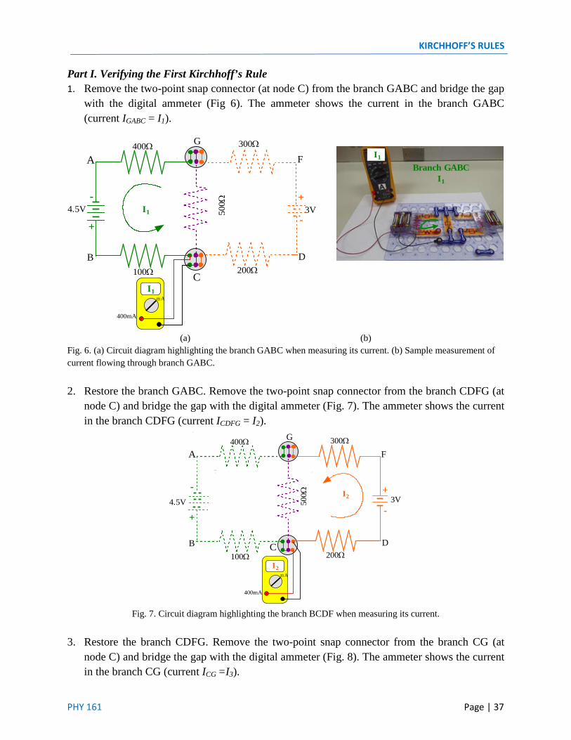
Part I. Verifying the First Kirchhoff’s Rule 1. Remove the two-point snap connector (at node C) from the branch GABC and bridge the gap
with the digital ammeter (Fig 6). The ammeter shows the current in the branch GABC (current IGABC = I1).
(a) (b) Fig. 6. (a) Circuit diagram highlighting the branch GABC when measuring its current. (b) Sample measurement of current flowing through branch GABC. 2. Restore the branch GABC. Remove the two-point snap connector from the branch CDFG (at
node C) and bridge the gap with the digital ammeter (Fig. 7). The ammeter shows the current in the branch CDFG (current ICDFG = I2).
400Ω
100Ω 200Ω
500Ω
4.5V 3V
A
C
G
B D
F
+
-
I2
I2mA
400mA
+
-
300Ω
Fig. 7. Circuit diagram highlighting the branch BCDF when measuring its current.
3. Restore the branch CDFG. Remove the two-point snap connector from the branch CG (at
node C) and bridge the gap with the digital ammeter (Fig. 8). The ammeter shows the current in the branch CG (current ICG =I3).
400Ω
100Ω 200Ω
500 Ω4.5V 3V
A
C
G
B D
F
I1
+
-+
-
300Ω
I1mA
400mA
I1
Branch GABCI1

LAB WORK 6
Page | 38 PHY 161
400Ω
100Ω 200Ω
500Ω4.5V 3V
A
C
G
B D
F
+
-+
-I3
I3mA
400mA
300Ω
Fig. 8. Circuit diagram highlighting the branch CG when measuring its current.
4. Repeat these measurements now for the currents IGABC, ICDFG and ICG at the junction G. Part II. Verifying the Second Kirchhoff’s Rule 1. Using the digital voltmeter, measure the voltages across each element of the loop ABCGA
(Fig. 9). Note magnitude and sign of the voltages with respect to the direction of the passing loop
(a) (b) Fig. 9. (a) Schematic highlighting loop 1, ABCGA and showing the measurements of voltages around this loop. (b) Sample measurement across 100 Ω resistor.
VCGV
400Ω
100Ω 200Ω
500Ω
4.5V 3V
A
C
G
B D
F
+
- +
-Path forLoop 1
300Ω
VGAV
VABV
V
VBC
VBC
Loop 1ABCGA

KIRCHHOFF’S RULES
PHY 161 Page | 39
2. Measure the voltages around loop CDFGC (Fig. 10). Note magnitude and sign of the voltages with respect to the direction of the passing loop.
Fig. 10. Schematic depicting the measurements of voltages around loop 2 ABFGA.
3. Measure the voltages around loop ABCDFGA (Fig. 11). Note magnitude and sign of the
voltages with respect to the direction of the passing loop.
Fig. 11. Schematic depicting the measurements of voltages around loop 3, ABCDFGA.
VGCV
400Ω
100Ω 200Ω50
0Ω4.5V 3V
A
C
G
B D
F
+
- +
-Path forLoop 2
300Ω
V
VFG
VCDV
VDFV
400Ω
100Ω 200Ω
500Ω4.5V 3V
A
C
G
B D
F
+
- +
-
Path for Loop 3
300Ω
V
VFGVGAV
VABV
VCDVV
VBC
VDFV

LAB WORK 6
Page | 40 PHY 161
Calculations 1. Verify the First Kirchhoff’s Rule. For each junction, calculate the sum of the currents
entering the node and the sum of the currents leaving the node. If the sums equal each other then the First Kirchhoff’s Rule is verified. Find percentage difference between these sums. This percentage difference shows the experimental error of your measurements.
2. Verify the Second Kirchhoff’s Rule. Calculate algebraic sum of the voltages for each loop. If the sums equal zero, the Second Kirchhoff’s Rule is verified. For each loop, calculate algebraic sum of the voltages on the batteries and compare it with the algebraic sum of the voltages on resistors. Find percentage difference between the magnitudes of these sums. This percent difference shows the experimental error of your measurements.
3. Using the Second Kirchhoff’s Rule and the sign convention as shown on Table I develop the equations for each closed loop of Fig. 9a, Fig 10 and Fig. 11 respectively. Substitute the
corresponding values of ε, R and I for each loop. Perform the algebraic sum for each loop; are the sums equal to zero?
Questions 1. However accurate you perform the measurements the sums of the measured voltages are
never exactly zero. What is the main culprit of this error? 2. However accurate you perform the measurements the sums of the current entering a junction
are never exactly equal to the currents leaving the junction. What is the main culprit of this error?
3. Evaluate the internal resistances of the batteries using the obtained data. 4. Calculate the electric power developed in the circuit you measured. 5. Could you calculate the electric power developed in the circuit, if the resistances of the
resistors are unknown? Explain.
PHY 161 Page | 41
LAB
WORK 7
SOURCES OF ELECTROMOTIVE FORCE IN DIRECT CURRENT
CIRCUITS
Objectives
Task 1. To study the operation of sources of electromotive force in DC circuits
Task 2. To study combinations of EMF sources in series and in parallel
Task 3. To learn how to measure the magnitude of electromotive force and internal resistance of
a source of electromotive source.
Physical Principles
A device, which produces potential difference and can generate electric current, is a source of
electromotive force (EMF). In simple terms, EMF is the potential difference E produced inside
the source. Any real EMF source (e.g. electric generator or battery) is made of materials of
certain resistivity and, as such, it possesses a certain electrical resistance r. This resistance is
termed internal resistance of EMF source. The electric current generated by an EMF source and
flowing though it has to overcome this resistance. Thus, the internal resistance of an EMF source
is always included in the total resistance of the circuit, in with this source works.
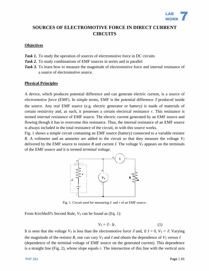
Fig. 1 shows a simple circuit containing an EMF source (battery) connected to a variable resistor
R. A voltmeter and an ammeter are added to the circuit so that they measure the voltage VT
delivered by the EMF source to resistor R and current I. The voltage VT appears on the terminals
of the EMF source and it is termed terminal voltage.
R
+ -
r
+
-
+
-
VT
I
Fig. 1. Circuit used for measuring ε and r of an EMF source.
From Kirchhoff's Second Rule, VT can be found as (Eq. 1):
VT = E - Ir. (1)
It is seen that the voltage VT is less than the electromotive force E and, if I = 0, VT = E. Varying
the magnitude of the resistor R, one can vary VT and I and obtain the dependence of VT versus I
(dependence of the terminal voltage of EMF source on the generated current). This dependence
is a straight line (Fig. 2), whose slope equals r. The intersection of this line with the vertical axis

LAB WORK 7
Page | 42 PHY 161
gives the value of E, while the intersection with the horizontal axis gives the value of the
maximum current Imax produced by the battery.
VT vs I
VT = -rI +
I
VT
Imax=x-intercept
=y-interceptV
T (
V)
I (A)
rI
Vslope T
Fig. 2. Dependence of terminal voltage on current.
EMF sources can be combined in series and in parallel. Series connection is used in order to
generate greater terminal voltages (Fig. 3).
R
+ -
+
-
VT
r
+
-
I- +
r
1
2
Fig. 3. Two batteries connected in series.
If two EMF sources of E1, r1 and E2, r2 are connected in series, the total electromotive force Eseries
and the total internal resistance rseries are just sums of the constituents (Eq. 2):
Eseries = E1 + E2,
rseries =r1 + r2. (2)
Parallel connection of EMF sources is used in order to increase the current, which can be
delivered to the circuit (Fig. 4).
SOURCES OF ELECTROMOTIVE FORCE IN DIRECT CURRENT CIRCUITS
PHY 161 Page | 43
R
+ -
+
-
VT
I
r
+
-
r
+
-
1 2
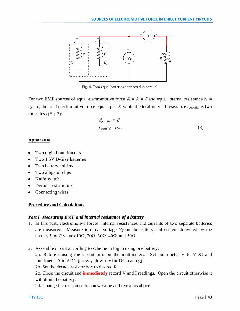
Fig. 4. Two equal batteries connected in parallel.
For two EMF sources of equal electromotive force E1 = E2 = E and equal internal resistance r1 =
r2 = r, the total electromotive force equals just E, while the total internal resistance rparallel is two
times less (Eq. 3):
Eparallel = E
rparallel =r/2. (3)
Apparatus
Two digital multimeters
Two 1.5V D-Size batteries
Two battery holders
Two alligator clips
Knife switch
Decade resistor box
Connecting wires
Procedure and Calculations
Part I. Measuring EMF and internal resistance of a battery
1. In this part, electromotive forces, internal resistances and currents of two separate batteries
are measured. Measure terminal voltage VT on the battery and current delivered by the
battery I for R values 10Ω, 20Ω, 30Ω, 40Ω, and 50Ω.
2. Assemble circuit according to scheme in Fig. 5 using one battery.
2a. Before closing the circuit turn on the multimeters. Set multimeter V to VDC and
multimeter A to ADC (press yellow key for DC reading).
2b. Set the decade resistor box to desired R.
2c. Close the circuit and immediately record V and I readings. Open the circuit otherwise it
will drain the battery.
2d. Change the resistance to a new value and repeat as above.

LAB WORK 7
Page | 44 PHY 161
Fig. 5. Circuit set-up for experimenting with single battery.
3. Plot the obtained data VT versus I (see Fig. 6 for Sample graph). Fit the experimental points
on the plot with a straight line. Find intersection of this line with the y-axis and take note of
the corresponding value E1. Find slope of the fitting straight line. This slope equals r1. Note
that on this experiment you will not be required to obtain the maximum current based on the
x-intercept of the graph.
VT (
V)
VT vs I
I (A)
VT = -0.378 I + 1.56
I
VT
=1.56V
slope=-r=-0.378
Imax=6.6A
Fig. 6. Sample graph of the terminal voltage as a function of current for a single battery.
R Decade
box
+
-
Switch
r
V DC
V
V
A
A DC
A
10A
Set dial to
V DC
Set dial to A
press yellow
key for DC
Keep the circuit open till ready to take data
Set R to
desired value
Switch is up

SOURCES OF ELECTROMOTIVE FORCE IN DIRECT CURRENT CIRCUITS
PHY 161 Page | 45
4. Disconnect the battery from the circuit and measure the voltage on its terminals using a
voltmeter (Fig. 7). This voltage equals E1 measured directly. Compare E1 values obtained in
steps 2 and 3, find average value of E1 and calculate percentage difference.
Fig. 7. Direct measurement of electromotive force of a battery using voltmeter.
5. Repeat the steps 1 to 4 for another battery and obtain values E2 and r2 for this battery.
Compare E1, and E2, r1 and r2.
Part II. Two batteries connected in series
In this part, electromotive force, internal resistance and current of two batteries connected in
series are measured.
1. Assemble two batteries in series and repeat the previous procedure for this new configuration
(Fig. 8). Plot the corresponding graph and obtain the values Eseries and rseries.
Fig. 8. Circuit set-up for two batteries connected in series
2. Using a voltmeter, measure the voltage directly on the terminals of the series assembly. This
voltage is the experimental value of the electromotive force of two batteries connected in
series Eseries.
+
-
Switch
V DC
V
V
A
A DC
A
10A
1
2
rr
R

LAB WORK 7
Page | 46 PHY 161
3. Calculate sum of the electromotive forces of the individual batteries E1, and E2 you measured
in the previous procedure. This sum is the calculated value of Eseries. Compare the calculated
and experimental values of Eseries and calculate the percentage difference between them.
4. Compare Eseries with E1, and E2 and make a conclusion.
Part III. Two batteries connected in parallel
In this part, electromotive force, internal resistance and current of two batteries connected in
parallel are measured.
1. Assemble two batteries in parallel and repeat the previous procedure now for two batteries
connected in parallel (Fig. 9). Plot the corresponding graph and obtain the values Eparallel, and
rparallel.
Fig. 9. Circuit set-up for two batteries connected in parallel.
2. Using a voltmeter, measure the voltage directly on the terminals of the parallel assembly.
This voltage is the experimental value of the electromotive force of two batteries connected
in series Eparallel.
3. Compare all obtained experimental and calculated values of Eparallel, E1 , E2; and rparallel r1, r2
and make a conclusion.
Questions
1. Is every electromotive force a potential difference? Explain.
2. Is every potential difference an electromotive force? Explain.
3. What are the advantages and disadvantages of connecting batteries in series?
4. What are the advantages and disadvantages of connecting batteries in parallel?
5. What would happen if you alter the polarity of one of the batteries in Fig. 3?
6. How many batteries are needed in order to increase both EMF and the maximum current?
How the batteries must be connected in order to achieve this?
+
-
Switch
V DC
V
V
A
A DC
A
10A
r r R1 2

PHY 161 Page | 47
LAB
WORK 8
RC CIRCUITS
Objective
To study the processes of charging and discharging of a capacitor in RC circuit and determine
time constant of these processes.
Task 1: Measure resistance and capacitance of an RC circuit and calculate its time constant.
Task 2: Obtain charging and discharging curves
Physical Principles
RC circuits are DC circuits composed of resistors, EMF sources and capacitors. In RC circuits, in
contrast to DC circuits without capacitors, currents do not reach their constant values
momentarily, but in a certain time, which is required to charge capacitors. This time is a
characteristic of an RC circuit and is known as time constant τ. For a rudimentary RC circuit
containing one resistor of resistance R, one capacitor of capacitance C and one EMF source of
magnitude E, time constant equals product of R and C (Eq. 1):
τ = RC. (1)
Voltage across the capacitor Vc during the process of its charging increases with time t from zero
to E and is described by the formula (Eq. 2):
Vc = E [1 – exp(-t/τ)]. (2)
The graph below in Fig. 1a shows the dependence of the voltage across a capacitor versus time
during the process of charging. According to the formula (2), at time t = τ, the voltage across the
capacitor reaches a value of Vτ.charge = 0.63E.
Vm
Vm
V = 0.37 Vm
VC (V)
V = 0.63 Vm
VC (V)
(a) (b) Fig. 1. Development of voltage across capacitor in an RC circuit: (a) the process of charging; (b) the process of
discharging.
LABWORK 8
Page | 48 PHY 161
When the EMF source is switched off, the capacitor loses its charge and voltage on capacitor Vc
goes down. The capacitor discharges. The characteristic time of the discharge, its time constant,
has the same value: τ = RC. Yet, the change of Vc in time is described by a different formula (Eq.
3):
Vc = E exp(-t/ τ)] (3)
Fig. 1b shows the change of voltage across a capacitor during the process of discharge. Initially,
the voltage equals E and then it goes down approaching zero. At time t = τ, the voltage across the
capacitor reaches a value of Vτ.discharge = 0.37E.
Apparatus
Digital multimeter
Two AA batteries and battery holder
Snap-circuit 470 μF and 100 μF capacitors
Two snap-circuit 10 kΩ resistors
Snap-circuit SPDT Switch
Snap-circuit connectors and one snap-to-snap wire connector
Large snap-circuit board
Vernier voltage sensor
Labquest2 interface and LoggerPro software
Preliminary set-up:
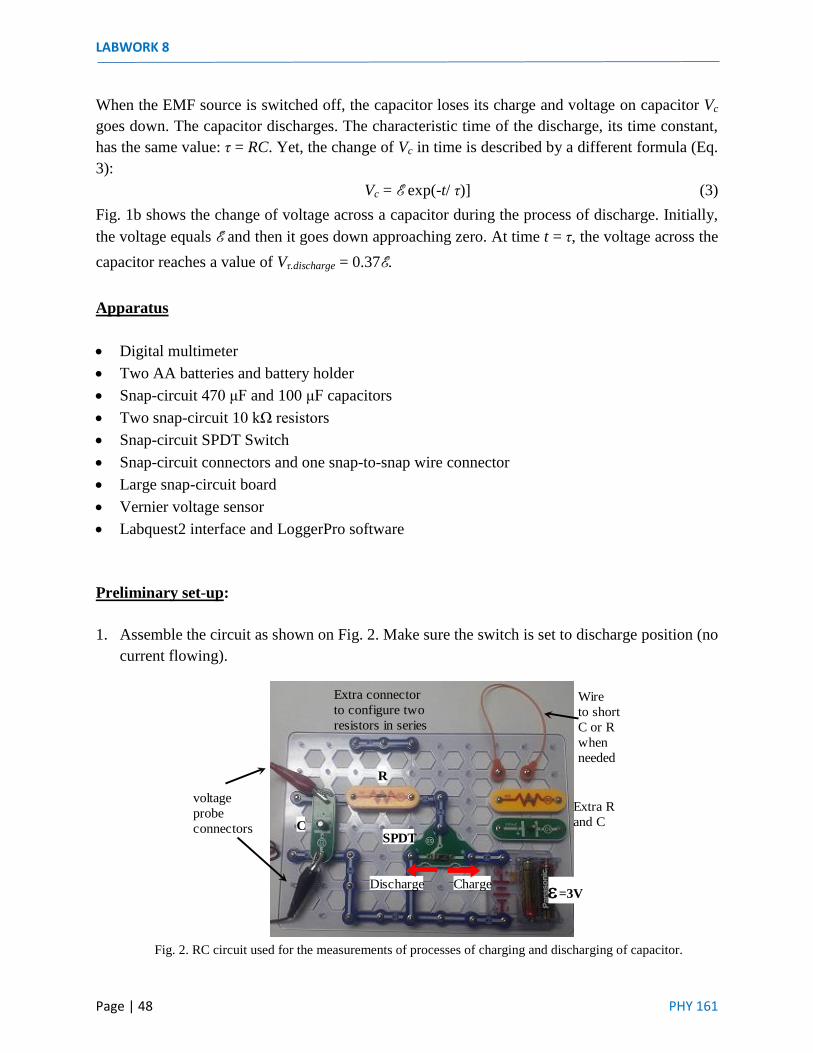
1. Assemble the circuit as shown on Fig. 2. Make sure the switch is set to discharge position (no
current flowing).
Fig. 2. RC circuit used for the measurements of processes of charging and discharging of capacitor.
ChargeDischarge
voltage
probe
connectors
Wire
to short
C or R
when
needed
C
R
SPDT
=3V
Extra R
and C
Extra connector
to configure two
resistors in series

RC CIRCUITS
PHY 161 Page | 49
2. By means of a multimeter measure the actual resistance of each 10 kΩ resistor, actual
capacitance of the 470 µF and 100 µF capacitors, and the total emf of the batteries. Note that
each component must be disconnected from the circuit before performing each measurement.
3. Turn on the Labquest2 interface unit. Connect the voltage sensor to Ch1. Connect the
interface to a computer by means of a USB cable.
4. Open the LoggerPro program. A graph window will open up with Potential vs Time axes.
5. Double-click on the Potential column. Rename it: Vc. Click Ok.
6. Click on Data Collection and enter the information as per the table below. Note that Data
Collection settings will depend on the capacitor and resistor in your circuit.
Table I
Circuit 1
470 µF and 10 kΩ
Circuit 2
470 µF and 20 kΩ
Circuit 3
100 µF and 10 kΩ
Duration: 60 seconds Duration: 60 seconds Duration: 20 seconds
Sampling Rate: 500 Sampling Rate: 500 Sampling Rate: 500
Procedure:
Circuit 1 - 470 µF and 10 kΩ:
Charging:
1. With the switch in discharge position zero the voltage probe
Click on the “triggering” tab and select the triggering box
Select “Increasing”
Enter 0.005
Click OK
2. Click COLLECT, a message will pop-up: “Waiting for Trigger”
3. Immediately, throw the switch to charging position (towards the battery). The program will
collect data for 60 seconds and stop on its own. Keep the switch on the charging position.
4. Click on “Experiment” and select “Store Latest Run.”
Discharging:
1. With the switch still in the charging position (DO NOT zero the probe)
From the data table record the voltage at which charging stopped.
Click on Data Collection and select the triggering tab
Select “Decreasing”
Enter a value that is 0.010 or 0.020 lower than the stored voltage in your capacitor.
Click OK
2. Click COLLECT, a message will pop-up: “Waiting for Trigger”
LABWORK 8
Page | 50 PHY 161
3. Throw the switch to discharging position (away from the battery). The program will collect
data for 60 seconds and stop on its own.
4. Click on “Experiment” and select “Store Latest Run.”
Circuit 2 - 470 µF and 20 kΩ:
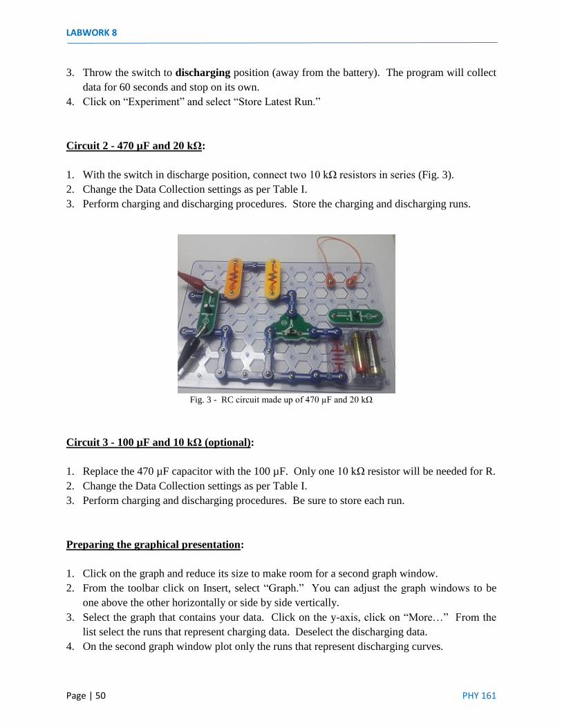
1. With the switch in discharge position, connect two 10 kΩ resistors in series (Fig. 3).
2. Change the Data Collection settings as per Table I.
3. Perform charging and discharging procedures. Store the charging and discharging runs.
Fig. 3 - RC circuit made up of 470 µF and 20 kΩ
Circuit 3 - 100 µF and 10 kΩ (optional):
1. Replace the 470 µF capacitor with the 100 µF. Only one 10 kΩ resistor will be needed for R.
2. Change the Data Collection settings as per Table I.
3. Perform charging and discharging procedures. Be sure to store each run.
Preparing the graphical presentation:
1. Click on the graph and reduce its size to make room for a second graph window.
2. From the toolbar click on Insert, select “Graph.” You can adjust the graph windows to be
one above the other horizontally or side by side vertically.
3. Select the graph that contains your data. Click on the y-axis, click on “More…” From the
list select the runs that represent charging data. Deselect the discharging data.
4. On the second graph window plot only the runs that represent discharging curves.

RC CIRCUITS
PHY 161 Page | 51
Calculations
Find the best fit for both charging and discharging experimental data:
1. Select the Charging Graph:
Fit the data on the graph with the dependence y = A(1 – exp(-x/B)). Click on f(x) on the top
toolbar, select “Zaitsev Charging” A*(1-exp(-t/B)). Click Try Fit, click OK. Record the
parameters A and B, which equal E and τ respectively. If the function is not available select
“Inverse Exponent,” click “Define Function.” In the box type: A(1– exp(-t/B)), click OK.
Click Try Fit. Click OK.
2. Select the Discharging Graph:
Fit the data on the graph with the dependence y = A exp(-x/B). Click on f(x) on the top
toolbar, select “Zaitsev Discharging,” A*exp(-t/B). Click Try Fit, click OK. Record the
parameters A and B, which equal E and τ respectively. If the function is not available select
“Natural Exponent,” click on “Define Function.” In the box type: A*exp(-t/B), click OK.
Click Try Fit. Click OK.
3. Calculate Vτ.charging = 0.63E for the charging process and on the charging graph find the
corresponding time. This time is the time constant τ (Fig. 1).
4. Calculate Vτ.discharging = 0.37E for the discharging process and on the discharging graph find
the respective time for this voltage. This time equals the time constant τ (Fig. 2).
5. Knowing that τ = RC, where R and C are the values of the resistance and capacitance used in
this experiment, calculate time constant and compare the calculated value with the
experimental ones. Calculate the percentage difference between them.
6. Once data analysis is complete and all printing has been done disconnect the LabQuest2 unit
from the computer. Turn off the interface by pressing the Home key, tap on System then tap
on Shut Down. Remove the voltage sensor. Put all instruments and equipment away as
directed by your instructor and/or technician.
Questions
1. Compare the experimental time constants measured in the charging and discharging
processes. Which value is greater and why is it greater?
2. Does the time constant depend on the voltage delivered by the battery?
3. Based on the parameters of the experiment determine the maximum charge accumulated on
the capacitor.
4. Based on the parameters of the experiment determine the maximum current flowing through
the resistor.
5. For this experiment, show a simple way of measuring the resistance of the multimeter.

LABWORK 8
Page | 52 PHY 161

PHY 161 Page | 53
LAB WORK 9
MAGNETIC FIELD OF A SLINKY SOLENOID (In part, adapted from Vernier’s “Physics with Computers” lab manual)
Objective To experimentally study the magnetic field produced by a solenoid. Task 1: Measure the magnitude of magnetic field in a solenoid as a function of the current
passing through it. Task 2: Measure the magnitude of magnetic field in a solenoid as a function of its length. Task 3: Measure the magnitude of magnetic field in a solenoid as a function of density of its
turns. Physical Principles A solenoid is a long coil of wire with many loops (turns). If current passes through the wire, a magnetic field is produced inside and around the solenoid (Fig. 1).
I I
Fig.1. Distribution of magnetic field produced by a simple solenoid. The red arrows show current flowing in solenoid. Magnetic field concentrates inside solenoid and becomes negligibly small outside solenoid. Inside a solenoid, the magnitude field is uniform and its strength B can be found as (Eq. 1):
𝑩 = µ𝟎𝑵𝑳𝑰 , (1)
where L is the length of the solenoid, N is the number of wire loops, I is the current passing through the wire of the solenoid and µ0 is the magnetic permeability of space (µ0 = 1.26×10⁻⁶ Tm/A). Formula (1) shows that the magnetic field of a solenoid is proportional to the current passing through the solenoid (Fig. 2a). Thus, the strength of the magnetic field created in a solenoid can be described as a linear function of current (Eq. 2). The slope of this function ABI equals µ0N/L.
B = ABII. (2)

LAB WORK 9
Page | 54 PHY 161
The magnitude of magnetic field B is inversely proportional to the solenoid length L (Fig. 2b). Thus, this dependence can be presented by a hyperbolic function (Eq. 3), where the coefficient of proportionality ABL equals µ0NI.
B = ABL/L. (3) The magnitude of magnetic field B is also proportional to the number of turns N and, consequently, to the linear density of turns n = N/L (Fig. 2c). That is:
B = ABnn, (4) where the coefficient ABn equals µ0I.
(a) (b) (c)
Fig. 2. Dependence of the strength of magnetic field of a solenoid on (a) current, (b) solenoid length and (c) linear density of turns. In this lab work, a metal slinky serves as a solenoid. A solenoid made this way allows to easily change its length and hence, study the dependence of magnetic field of a solenoid on its length. Apparatus • Power supply • Metal slinky • Digital multimeter (A) • DPDT switch • 3 short, 2 black connecting wires • Two long connecting wires with alligator clips • Meter stick • Masking tape • 1 right angle clamp, 1 small table clamp with rod • Four weights (500 g, preferably brass) • Cardboard holders • Vernier LabQuest2 interface and magnetic field sensor • LoggerPro software

MAGNETIC FIELD IN A SLINKY SOLENOID
PHY 161 Page | 55
Procedure Preliminary Settings 1. Set-up slinky and Vernier LabQuest2 interface as shown on Fig. 3.
Fig. 3. (a) Diagram of the experimental set-up.
Fig. 3. (b) Assembly of the experimental set-up with the components provided. 2. Place the magnetic field sensor between the turns of the slinky near its center. Align the
sensor so that the white dot points directly down the long axis of the solenoid. 3. Turn on the power supply and the multimeter. Set the multimeter dial to position A and press
the yellow key for DC reading. 4. Close the circuit by throwing the switch towards the power supply. This allows for current to
flow through the slinky. Set the current to 2.0 A, to do this turn the voltage knob only and watch the current display on the multimeter until reaches 2.0A or a value very close to it. Open the circuit by setting the switch on the DPDT in central position (off position) again. Make sure that the ammeter reads zero current.
A
A DC
A
Metal Slinky
Connecting wire withAlligator clip
LabQuest2USB to computer
Vernier Interface
Ch1
Power supply
DPDTSwitch
Magnetic Field Sensor
Meter stick
LoggerPro
V A
10A
- +

LAB WORK 9
Page | 56 PHY 161
5. In order to confirm that the magnetic field probe is properly aligned, follow these steps: Double-click on the “Physics” icon and open LoggerPro 3.10. The interface will automatically detect the sensor and open a window with a Magnetic Field vs. Time graph. Click Collect to begin data collection. Wait a few seconds and close the circuit by throwing the switch towards the power supply or to a position that shows a positive current on the multimeter. If the magnetic field is positive and it is at its maximum, you are ready to take data. This will be the position of the sensor for all the measurements of the magnetic field for the rest of the lab work. If the field decreases when you throw the switch, rotate the sensor so that the white dot points the opposite direction down the solenoid. Turn the current off by throwing the switch to the center position.
Part I. Strength of Magnetic Field in Solenoid versus Current 1. Measure total length of the slinky solenoid L. 2. Open the “Physics” folder, open “PHY Exp Templates” folder, open “LoggerProTemplates”
folder, open “Magnetic Field Slinky” file. 3. With the switch in the center position click on the “Zero” button. No current should be
flowing through the circuit when zeroing the probe! When zeroing the probe, the contribution of the magnetic field of Earth, or any other random magnetic fields in the lab is subtracted from the reading.
4. Close the circuit and allow the previously set 2 A current to flow through the circuit. Click “Collect” to begin data acquisition.
5. When ready, click the “Keep” button; allow the probe to collect data for about 10 seconds. When prompted, enter the current reading from the multimeter (not from the power supply!) and press “OK” to accept the value you entered.
6. Decrease the current in 0.5 A steps until you reach 0.5 A and repeat as above each step. For a current of 0.0 A throw the switch to the OFF position and collect the corresponding magnetic field. Throw the switch to the opposite polarity to obtain negative magnetic fields for each value of I. Keep collecting data from 0.5 A to 2 A in steps of 0.5. Note that once you throw the switch to the opposite side, the values should be entered as negative currents such as -0.5, -1.0 and so on just as shown by the multimeter.
7. When you finish collecting data, click “Stop” and throw the switch to the central position. 8. Click on the graph window to select it. If needed, autoscale the graph by right-clicking on the
graph and selecting “Autoscale”. Determine the slope of the plotted data by clicking “f(x)” on the toolbar and selecting “proportional” fit. Click on “Try Fit”, click “OK”. See Fig. 4 for sample graph. Print the B vs. I graph and the data table together in landscape format.
9. Take note of the coefficient A on this graph. It is the coefficient ABI in Formula (2).

MAGNETIC FIELD IN A SLINKY SOLENOID
PHY 161 Page | 57
Fig. 4. Sample graph of magnetic field of slinky solenoid vs current.
Part II. Strength of Magnetic Field versus Solenoid Length and Density of Turns 1. In this procedure, the current remains constant throughout the entire data collecting process.
The sensor must be kept between the turns of the Slinky and near its center (as in Part I). 2. Count the number of loops in your slinky and record it as N. 3. Using the same template as in Part I double-click on the “Current” column and change the
name to “Length” and short name to “L” with units as [m]. Click “Ok.” 4. Close the circuit and set the current to 1.5 A. Open the circuit so multimeter reads 0.0 A.
With the magnetic field sensor in position and no current flowing through the circuit, click on the “Zero” button.
5. Click “Collect,” a dialog window will pop-up, from which you will click on the “Erase and Continue” tab. This will delete the previous data. Immediately, close the circuit. After a few seconds click “Keep” and enter the length at that point. Click “OK” to approve.
6. Change the length of the slinky and enter the new length by clicking “Keep”. To change the length, move your slinky inward in steps of 5 cm from each end so that you decrease the length in steps of 10 cm each time (Fig. 5). Do not remove the alligator clips, the total number of loops should remain the same throughout the experiment.
Fig. 5. Changing length of slinky solenoid.
Probe remains fixed at the center
Push slinky inward 0.05m from eachend. Thus changing L in steps of 0.1meach time. Change L from 1m to 0.4m.
Current remains constant

LAB WORK 9
Page | 58 PHY 161
7. Click “Stop” and open the circuit when you finish collecting data. Click on “f(x)” and select the inverse fit function A/L. Click “Try Fit” then click “OK”. See Fig. 6a for sample graph. Print the B vs. L graph and the data table together in landscape format. Note of the coefficient A on this graph is the coefficient ABL in Formula (3).
Fig. 6. (a) Sample graph of magnetic field of solenoid versus its length. It is a hyperbolic dependence with the coefficient of proportionality A = ABL. (b) Magnetic Field versus density of turns. Sample graphed data. It is a linear dependence with the coefficient of proportionality A = ABn. 8. From the top toolbar click on “Data” and select “Calculated Column”. Label it “n” and units
will be [turns/m]. In the expression box enter your number of turns and divide by L (either type “L” (with quotes) or click the “Variables” tab and select L). Click on the options tab and on the “displayed precision” option choose “1 decimal.”
9. On the Magnetic Field vs Length graph point at the x-axis where it says Length and change from L to n. This will plot data as Magnetic Field vs n. Autoscale from zero if needed. Click on “f(x)” and determine the slope of the line by using the proportional fit. See Fig. 6b for sample graph. Print the graph and data table together in landscape form. Take note of the coefficient A which is the coefficient ABn in Formula (4).
Calculations 1. Using the obtained value of the coefficient ABI, calculate the magnetic permeability of free
space µ0: µ0 = ABIL/N.
2. Using the obtained value of the coefficient ABL, calculate the magnetic permeability of free
space µ0: µ0 = ABL/(IN).
3. Using the obtained value of the coefficient ABn, calculate the magnetic permeability of free
space µ0: µ0 = ABn/I.

MAGNETIC FIELD IN A SLINKY SOLENOID
PHY 161 Page | 59
4. Find the average of the three calculated values of µ0 and compare the result with the known (rated) value: µ0 = 4π×10 −7 T∙m/A = 1.26×10⁻⁶ Tm/A. Calculate percentage difference between your measured average µ0 and the rated value µ0. This percentage difference is the experimental error of your measurements.
Questions 1. Does the magnetic field outside solenoid depend on the distance from the solenoid? 2. How the magnetic field inside solenoid depends on the solenoid diameter? 3. What would happen to the magnetic field inside a solenoid if it is bent? 4. Can you identify North and South poles of the solenoid you studied? 5. How can you prove experimentally that the magnetic field inside a solenoid is uniform?

LAB WORK 9
Page | 60 PHY 161

PHY 161 Page | 61
LAB
WORK 10
ALTERNATING CURRENT CIRCUITS
Objective
To learn basic principles of alternating current circuits comprising resistors, capacitors and
inductors.
Task 1: Measure reactance of capacitor in RC circuit as a function of frequency.
Task 2: Measure reactance of inductor in RL circuit as a function of frequency.
Task 3: Measure resonance frequency of rudimentary RLC circuit.
Physical Principles
In DC circuits with given EMF sources, the current flow is determined by resistors only. In DC
circuits, capacitors work just as circuit brakes, while inductors work like connecting wires. In
AC circuits, however, all three elements (resistors, capacitors and inductors) transmit current and
reveal certain resistances. Resistance of a resistor remains the same in any circuit, DC or AC. In
contrast, the resistance of a capacitor, or of an inductor, strongly depends on the frequency of AC
current. In order to distinguish the frequency dependent resistance of capacitors and inductors
from the frequency independent resistance of resistors, the former is termed reactance and
usually is denoted with capital letter X. Reactance XC of a capacitor of capacitance C and
reactance XL of an inductor of inductance L can be found as:
𝑿𝑪 =1
2𝜋𝒇𝑪 , (1)
𝑿𝑳 = 2𝜋𝒇𝑳 , (2)
where f is the frequency of AC current flowing through capacitor and/or inductor. According to
Ohm’s Law, the voltages on resistor, capacitor and inductor can be found as:
VR = I R,
VC = I XC, (3)
VL = I XL,
where I is the AC current.
Total resistance of an AC circuit composed of resistors, capacitors and inductors is called
impedance and it is denoted with letter Z. Accordingly, Ohm's law for AC current yields:
𝑰 =𝑽
𝒁, (4)
For an AC circuit with resistor, capacitor and inductor connected in series, the impedance can be
found as:
𝒁 = √𝑹2 + (𝑿𝑪 − 𝑿𝑳)2. (5)

LAB WORK 10
Page | 62 PHY 161
The total voltage drop across resistor, capacitor and inductor connected in series can be
calculated using the formula similar to Eq. 5, that is:
𝑽 = √𝑽𝑹2 + (𝑽𝑳 − 𝑽𝑪)2. (6)
Fig. 1 shows the simplest AC circuit comprising AC generator, resistor, capacitor and inductor
connected in series.
R
C
L
Vo
V
VL
v~
Fig. 1. AC circuit comprising AC generator, resistor, capacitor and inductor connected in series. Digital voltmeter is
shown connected to the inductor for the measurement of voltage VL.
Combining equations (1-5), one obtains an explicit formula for the current I passing through an
AC circuit composed of resistor, capacitor and inductor connected in series:
𝑰 =𝑽
𝒁=
𝑽
√𝑹𝟐 + (2𝜋𝒇𝑳 −1
2𝜋𝒇𝑪)
2
. (7)
The formula (6) shows that the current in AC circuit depends on frequency (Fig. 2).
Fig. 2. Dependence of current in a simple RLC circuit on frequency. At a certain frequency (the resonance frequency
fr), the current reaches its maximum. The smaller the resistance of the resistor in the circuit the more pronounced the
current maximum.
At a certain frequency fr, (resonance frequency), the current reaches its maximum. This
condition is known as resonance of AC circuit. At the resonance frequency, the reactance of
capacitor becomes equal to the reactance of inductor XC = XL, and the total impedance of the

ALTERNATING CURRENT CIRCUITS
PHY 161 Page | 63
circuit reaches its minimum (Z = R). The resonance frequency depends on the magnitudes of C
and L and can be found as:
𝒇𝒓 =1
2𝜋√𝑳𝑪 (8)
For an AC circuit composed of resistor and capacitor only (RC circuit), the equation 7 is
simplified to:
𝑰 =𝑽
√𝑹𝟐 + (1
2𝜋𝒇𝑪)
2
= 𝑽𝑪
𝑿𝑪= 2𝜋𝒇𝑪𝑽𝑪. (9)
Thus, in RC circuits, the current increases with frequency (Fig. 3a).
Fig. 3. (a) Current in a RC circuit as a function of frequency: current is increasing with frequency. (b) Current in a
RL circuit as a function of frequency: current is decreasing with frequency.
For an AC circuit composed of resistor and inductor only (RL circuit), current can be found as:
𝑰 =𝑽
√𝑹𝟐 + (2𝜋𝒇𝑳)2=
𝑽𝑳
𝑿𝑳=
𝑽𝑳
2𝜋𝒇𝑳. (10)
Thus, in RL circuits, the current decreases with the frequency (Fig. 3b).
Apparatus
Function generator
Digital multimeter (A)
Digital multimeter (V)
Snap-circuit board and connectors
100 Ω resistor
10 µF capacitor
Cu
rren
t
Cu
rren
t
Frequency Frequency
(a) (b)
RC RL

LAB WORK 10
Page | 64 PHY 161
10 mH radial inductor
Miniature 2.5V bulb
Multimeter with inductance measurement capability
Connecting wires, alligator clips, banana-to-snap connectors, switch.
Procedure and Calculations
Preliminary settings
1. Examine the resistor, capacitor and inductor given for this lab work and measure their actual
resistance R, capacitance C and inductance L using the multimeter. Take note of the obtained
values.
2. Assemble the circuit shown in Fig. 4.
V
Vo
v~
Hz
V
A
mA
400mA
Extra 3pt snap connector
Function
Generator
100 10 F 10 mH
OFF 2.5 V Bulb
Fig. 4. Composition of RCL circuit studied in this lab work. The nominal values of resistance, capacitance and
inductance are shown.
Part I. RC Circuit
1. Assemble an RC circuit of a resistor and a capacitor connected in series (Fig. 5). Note that
the RC circuit is just a simplified RCL circuit shown in Fig. 4.
Hz
V
A
mA
400mA
Function
Generator
100 10 F
OFFV
VC
v~
Fig. 5. RC Circuit. Measuring voltage VC on capacitor and current I flowing through the circuit.
2. Measure voltage VC on capacitor and current I in the circuit in the frequency range from 400
to 1000 Hz in steps of 100 Hz. Take note of the measured values.

ALTERNATING CURRENT CIRCUITS
PHY 161 Page | 65
3. Using the obtained data plot graph I versus f. Note that the current increases as the frequency
increases (Fig. 6a).
(a) (b)
Fig. 6. (a) Sample data of current I versus frequency f. (b) Reactance of the capacitor XC versus frequency f. The
experimental data are fitted with function y(f) = 1/(2πCx). The fitting parameter C equals the capacitance C.
4. Plot graph XC versus f and fit the data with function y(f) = 1/(2πCf) (Fig. 6b). Take note of
the fitting parameter C. The value of C equals the magnitude of the capacitance C.
5. Compare the obtained value of C with that you have measured directly with multimeter and
calculate the percentage difference. This difference is your experimental error.
Part II. RL Circuit
1. Assemble an RL circuit of resistor and inductor connected in series (Fig. 7). Note that the RL
circuit is just a simplified RCL circuit shown in Fig. 4.
V
VL
v~Hz
V
A
mA
400mA
Function
GeneratorOFF
100 10 mH
Fig. 7. RC Circuit. Measuring voltage VL on capacitor and current I flowing through the circuit.

LAB WORK 10
Page | 66 PHY 161
2. Measure voltage VL on inductor and current I in the circuit in the frequency range from 400
to 1000 Hz in steps of 100 Hz. Take notes of the measured values.
3. Using the obtained data plot graph I versus f. Note that the current decreases with frequency
(Fig. 8a).
(a) (b)
Fig. 8. (a) Sample data of current I vs frequency f in RL circuit. (b) Reactance of the inductor XL vs frequency f. The
experimental data are fitted with a function y(f) = 2πLf. The fitting parameter L equals the inductance L.
4. Plot graph XL versus f and fit the data with function y(f) = 2πLf (Fig. 8b). Take note of the
fitting parameter L. The value of L equals the magnitude of the inductance L.
5. Compare the obtained value of L with that you have measured directly with multimeter and
calculate the percentage difference. This difference is your experimental error.
Part III. RCL Circuit
1. Assemble an RCL circuit of resistor, capacitor and inductor connected in series (Fig. 4).
2. Measure the current in the circuit at frequencies from 200 to 600 Hz in steps of 50 Hz them
from 600 Hz to 1200 in steps of 100 Hz. Take note of the measured values.
Hz
V
A
mA
400mA
Function
GeneratorOFF
2.5 V Bulb 10 F 10 mH
Fig. 9. RCL Circuit. Measuring the current I flowing through the circuit.
3. Tuning the frequency, find the maximum current and record both the frequency and current.

ALTERNATING CURRENT CIRCUITS
PHY 161 Page | 67
4. With the signal generator still set to the frequency that provided maximum current set the
circuit as shown on Fig. 10. Measure voltages on capacitor VC and inductor VL . Take note
of the measured values.
Hz
Function
Generator
2.5 V Bulb 10 F 10 mH
OFFV
VC
v~
V
VL
v~
Fig. 10. RCL Circuit. Measuring voltage VC on the capacitor, voltage VL on inductor.
5. Using the obtained data plot current I versus frequency f (Fig. 11).
Fig. 11. Sample dependence of current I versus frequency f in RLC circuit. The current reaches maximum at the
resonance frequency.
6. On the graph, find the frequency, at which current reaches maximum. This is the resonance
frequency fr. Take note of this frequency.
7. Calculate the resonance frequency using formula (8) and find the percentage difference
between the calculated and measured values of fr. This difference is your experimental error.
8. For the resonance frequency, calculate the reactance of the capacitor XC (Eq. 1) and the
reactance of the inductor XL (Eq. 2). Compare the both values and calculate the percentage
difference between the two. This difference is your experimental error.
9. Compare voltages VC and VL you have measured at the resonance frequency and calculate the
percentage difference between the two values. This difference is your experimental error.

LAB WORK 10
Page | 68 PHY 161
Questions
1. What happens to the reactance of capacitor, reactance of inductor and the resistance of
resistor when frequency increases to the infinity?
2. What happens to the reactance of capacitor, reactance of inductor and the resistance of
resistor when frequency approaches zero?
3. Does the resonance frequency of an AC circuit depend on the voltage delivered by generator?
Explain your answer.
4. Does the resonance frequency depend on the magnitude of resistance R? Explain your
answer.
5. What is special about the voltages on capacitor and inductor at the resonance frequency?

PHY 161 Page | 69
LAB WORK 11
REFLECTION AND REFRACTION
Objective
To understand the phenomena of reflection and refraction of light, and to verify experimentally the laws of reflection and refraction. Task 1: Measure the angles of incidence and reflection and verify the law of reflection. Task 2: Measure the angles of incidence and refraction and verify the law of refraction. Task 3: Measure the index of refraction of acrylic plastic and water. Task 4: Measure the angle of total internal reflection for acrylic plastic and water. Task 5. Verify Snell’s law using the method of light beam shift.
Physical Principles
When a light beam strikes the surface of an object (incident beam), it splits into two parts: one is reflected from the surface (reflected beam) and the other one propagating inside the object (refracted beam) (Fig. 1).
Fig. 1. Interaction of light beam with an object: (a) plane surface and (b) curved surface. In both cases, the angle of incidence θi is that between the incident ray and the normal to the surface, whereas the angle of reflection θre is that between the reflected ray and the normal to the surface, and the angle of refraction θra is that between the refracted ray and the normal to the surface. The direction of propagation of the reflected beam is described by the law of reflection, while the direction of propagation of the refracted one is described by the law of refraction. It is important to understand the definition of the angles describing the directions of the beams: the angle of incidence θi , the angle of reflection θre and the angle of refraction θra. As it is seen in Fig. 1, all these angles are taken as angles between the corresponding beams and the normal with respect to the surface.
a
Θi
Θre
Θra
n1
n2
Θi Θ
re
b
Θra
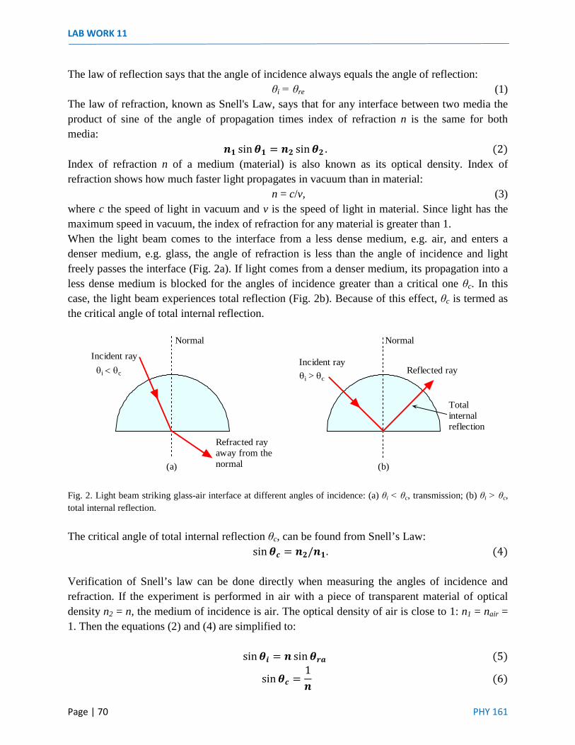
LAB WORK 11
Page | 70 PHY 161
The law of reflection says that the angle of incidence always equals the angle of reflection: θi = θre (1)
The law of refraction, known as Snell's Law, says that for any interface between two media the product of sine of the angle of propagation times index of refraction n is the same for both media:
𝒏𝟏 sin𝜽𝟏 = 𝒏𝟐 sin𝜽𝟐 . (2) Index of refraction n of a medium (material) is also known as its optical density. Index of refraction shows how much faster light propagates in vacuum than in material:
n = c/v, (3) where c the speed of light in vacuum and v is the speed of light in material. Since light has the maximum speed in vacuum, the index of refraction for any material is greater than 1. When the light beam comes to the interface from a less dense medium, e.g. air, and enters a denser medium, e.g. glass, the angle of refraction is less than the angle of incidence and light freely passes the interface (Fig. 2a). If light comes from a denser medium, its propagation into a less dense medium is blocked for the angles of incidence greater than a critical one θc. In this case, the light beam experiences total reflection (Fig. 2b). Because of this effect, θc is termed as the critical angle of total internal reflection.
Fig. 2. Light beam striking glass-air interface at different angles of incidence: (a) θi < θc, transmission; (b) θi > θc, total internal reflection. The critical angle of total internal reflection θc, can be found from Snell’s Law:
sin𝜽𝒄 = 𝒏𝟐/𝒏𝟏. (4) Verification of Snell’s law can be done directly when measuring the angles of incidence and refraction. If the experiment is performed in air with a piece of transparent material of optical density n2 = n, the medium of incidence is air. The optical density of air is close to 1: n1 = nair = 1. Then the equations (2) and (4) are simplified to:
sin𝜽𝒊 = 𝒏 sin𝜽𝒓𝒂 (5)
sin𝜽𝒄 =1𝒏
(6)
Reflected rayIncident ray
Normal
Totalinternalreflection
Incident ray
Normal
Refracted rayaway from thenormal(a) (b)
θi < θc θi > θc
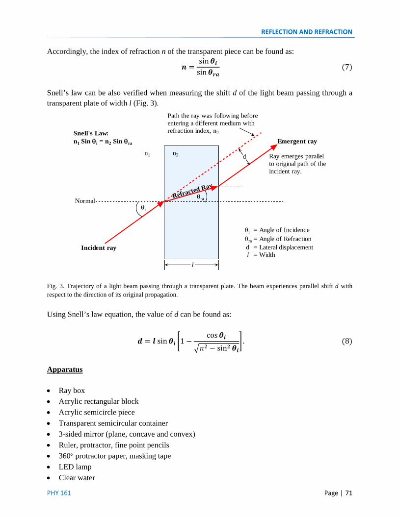
REFLECTION AND REFRACTION
PHY 161 Page | 71
Accordingly, the index of refraction n of the transparent piece can be found as:
𝒏 =sin𝜽𝒊
sin𝜽𝒓𝒂 (7)
Snell’s law can be also verified when measuring the shift d of the light beam passing through a transparent plate of width l (Fig. 3).
Fig. 3. Trajectory of a light beam passing through a transparent plate. The beam experiences parallel shift d with respect to the direction of its original propagation. Using Snell’s law equation, the value of d can be found as:
𝒅 = 𝒍 sin𝜽𝒊 1 −cos𝜽𝒊
𝑛2 − sin2 𝜽𝒊 . (8)
Apparatus
• Ray box • Acrylic rectangular block • Acrylic semicircle piece • Transparent semicircular container • 3-sided mirror (plane, concave and convex) • Ruler, protractor, fine point pencils • 360° protractor paper, masking tape • LED lamp • Clear water
n1 n2
Normal
Emergent ray
Incident ray
Refracted Ray
Ray emerges parallelto original path of theincident ray.
d
θra
θi
θi = Angle of Incidenceθra = Angle of Refractiond = Lateral displacementl = Width
Snell's Law:n1 Sin θi = n2 Sin θra
Path the ray was following beforeentering a different medium withrefraction index, n2
l
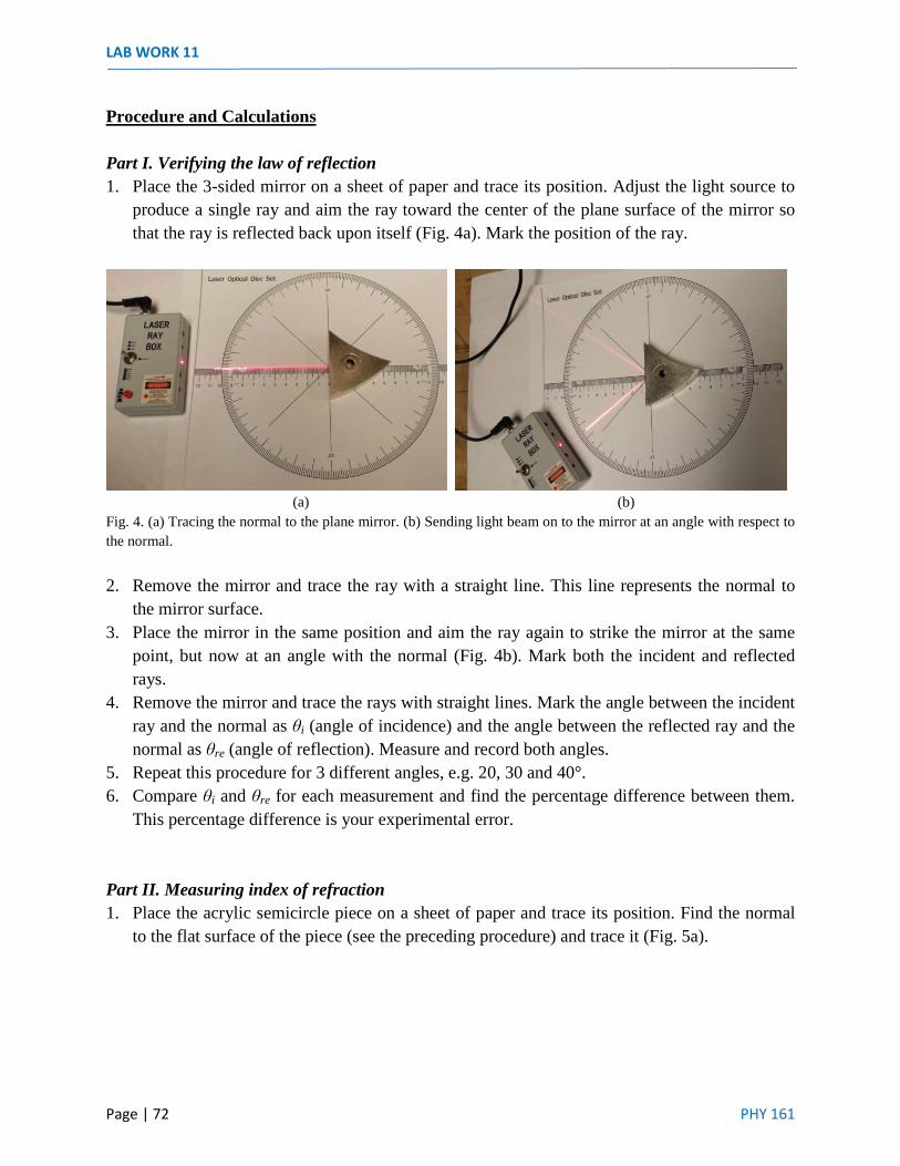
LAB WORK 11
Page | 72 PHY 161
Procedure and Calculations
Part I. Verifying the law of reflection 1. Place the 3-sided mirror on a sheet of paper and trace its position. Adjust the light source to
produce a single ray and aim the ray toward the center of the plane surface of the mirror so that the ray is reflected back upon itself (Fig. 4a). Mark the position of the ray.
(a) (b)
Fig. 4. (a) Tracing the normal to the plane mirror. (b) Sending light beam on to the mirror at an angle with respect to the normal. 2. Remove the mirror and trace the ray with a straight line. This line represents the normal to
the mirror surface. 3. Place the mirror in the same position and aim the ray again to strike the mirror at the same
point, but now at an angle with the normal (Fig. 4b). Mark both the incident and reflected rays.
4. Remove the mirror and trace the rays with straight lines. Mark the angle between the incident ray and the normal as θi (angle of incidence) and the angle between the reflected ray and the normal as θre (angle of reflection). Measure and record both angles.
5. Repeat this procedure for 3 different angles, e.g. 20, 30 and 40°. 6. Compare θi and θre for each measurement and find the percentage difference between them.
This percentage difference is your experimental error. Part II. Measuring index of refraction 1. Place the acrylic semicircle piece on a sheet of paper and trace its position. Find the normal
to the flat surface of the piece (see the preceding procedure) and trace it (Fig. 5a).

REFLECTION AND REFRACTION
PHY 161 Page | 73
(a) (b)
Fig. 5. (a) Tracing the normal to the flat surface of the semicircle acrylic piece. (b) Sending light beam on to the flat surface of the semicircle acrylic piece at an angle with respect to the normal. 2. Place the semicircle piece in its original position and aim the ray again to strike the flat
surface at the same point, but now at an angle θi with respect to the normal (Fig. 5b). Mark the incident and transmitted rays.
3. Trace the rays with straight lines and measure the angle of incidence θi and the angle of refraction θra.
4. Repeat this procedure for three different θi, e.g. 30, 40 and 50°. 5. Calculate the index of refraction n of acrylic for each pair of θi and θra using formula (7).
Find average value of n and the experimental error. 6. Repeat the procedure and calculations for the transparent container filled with clear water. Part III. Measuring the critical angle of total internal reflection 1. Place the semicircle acrylic piece on a sheet of paper and aim the light ray to the semicircle
surface of the piece so that the ray strikes the center of the flat surface. 2. Change the angle of incidence and observe the effects of transmission and internal reflection
from the flat surface of the acrylic (Fig. 6a).
(a) (b)
Fig.6. (a) Propagation of light beam through semicircle acrylic piece into air at angles of incident less than θc (transmission). (b) Propagation of light beam through semicircle acrylic piece and its reflection from the interface with air for the angles of incidence greater than θc (total internal reflection).

LAB WORK 11
Page | 74 PHY 161
3. Find the critical angle of incidence, at which the transmission through the acrylic piece into air disappears and trace the position of the light beam. This angle of incidence is the critical angle of total internal reflection θc.
4. Increase the angle of incidence and observe the effect of total internal reflection (Fig. 6b). Trace the incident and reflected rays and measure the angles of incidence and reflection. Compare both angles and calculate the percentage difference between them.
5. Calculate θc using formula (6) and compare the result with the angle θc you have measured experimentally. Calculate the percentage difference between two values. This percentage difference is your experimental error.
Part IV. Verifying Snell’s Law 1. Place the rectangular acrylic block on a sheet of paper and trace its position. Find the normal
to the longer surface of the block (see the preceding procedure) and trace it (Fig. 7a).
(a) (b)
Fig. 7. (a) Tracing the normal to the longer surface of the rectangular acrylic block. (b) Sending the light beam at an angle with respect to the normal. Note the shift of the beam after passing through the acrylic block. 2. Aim the ray again to strike the block at the same point, but now at an angle θi with respect to
the normal (Fig. 7b). Trace the incident and transmitted rays. 3. Remove the block and, using ruler, extend the rays so that you have two parallel lines and
clearly see the shift between them. 4. Draw a line perpendicular with respect to the parallel lines so that it intersects both parallel
lines. Measure the distance d between the lines (Fig. 8).

REFLECTION AND REFRACTION
PHY 161 Page | 75
n1 n2
Normal
Emergent ray
Incident ray
Refracted Ray
d
θra
θi
Air AcrylicRay box setto single rayoutput
l
Fig. 8. Drawing showing the shift d of the transmitted ray and the parameters l, θi and n used to calculate the value of d. 5. Repeat the procedure for three different θi. 6. Measure the block width l (Fig. 8) and calculate distance d using formula (8) for each θi.
Calculate the percentage difference between the measured and calculated values of d for each angle. Calculate average of these percentage differences. The obtained average percentage difference is your experimental error.
Questions
1. At the interface of two transparent media, light ray experiences both refraction and reflection. Does the angle of reflection depend on the angle of refraction?
2. Can you demonstrate the effect of total internal reflection using the rectangular block? Explain your answer and support your answer with a drawing.
3. In which case the shift of the light beam passing through the transparent block equals zero?

LAB WORK 11
Page | 76 PHY 161

PHY 161 Page | 77
LAB
WORK 12
SPHERICAL MIRRORS AND LENSES
Objective
To study the geometry of propagation of light reflected from spherical mirrors and light passing
through spherical lenses.
To learn the principles of measuring focal distance of spherical mirrors and lenses.
Task 1: Find the focal point and center of curvature of a concave mirror.
Task 2: Find the focal point and center of curvature of a convex mirror.
Task 3: Find and measure the focal lengths of a converging lens.
Task 4: Find and measure the focal lengths of a diverging lens.
Physical Principles
Based on their shapes and refracting properties mirrors and lenses are capable of forming images
of objects placed in front of them. There are two basic types of mirrors and lenses. The one is the
mirrors and lenses which convert initially parallel light rays in converging rays. The mirrors and
lenses of this type are known as concave mirrors and converging lenses. The mirrors and lenses
of the other type convert initially parallel light rays into diverging rays. These mirrors and lenses
are convex mirrors and diverging lenses. The simplest mirrors and lenses working as converging
and diverging optical elements are those with spherical surfaces (Fig. 1).
Fig. 1. (a) A convex mirror with spherical surface. (b) Converging lenses with spherical surfaces.
Spherical Mirrors
When parallel rays of light fall on a spherical concave mirror, upon reflection they pass through
one and the same point, which is known as focal point (Fig. 2a). Since in this point real light rays
merge, the focal point of concave mirrors is termed as real focal point. If the mirror is convex,
the initially parallel light rays diverge upon reflection and do not cross each other (Fig. 2b). Yet,
their extensions (virtual rays) to the back of the mirror do merge in one and the same focal point.
This point of concentration of the virtual rays is termed virtual focal point of convex mirror.
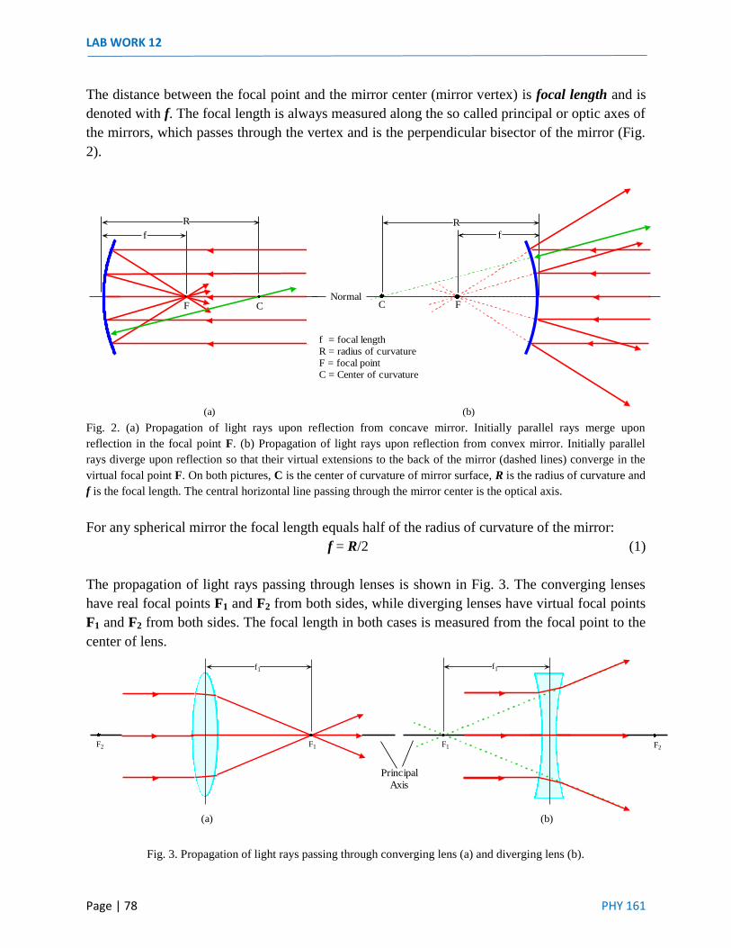
LAB WORK 12
Page | 78 PHY 161
The distance between the focal point and the mirror center (mirror vertex) is focal length and is
denoted with f. The focal length is always measured along the so called principal or optic axes of
the mirrors, which passes through the vertex and is the perpendicular bisector of the mirror (Fig.
2).
f = focal length
R = radius of curvature
F = focal point
C = Center of curvature
f
R
CFNormal
C F
f
R
(a) (b)
Fig. 2. (a) Propagation of light rays upon reflection from concave mirror. Initially parallel rays merge upon
reflection in the focal point F. (b) Propagation of light rays upon reflection from convex mirror. Initially parallel
rays diverge upon reflection so that their virtual extensions to the back of the mirror (dashed lines) converge in the
virtual focal point F. On both pictures, C is the center of curvature of mirror surface, R is the radius of curvature and
f is the focal length. The central horizontal line passing through the mirror center is the optical axis.
For any spherical mirror the focal length equals half of the radius of curvature of the mirror:
f = R/2 (1)
The propagation of light rays passing through lenses is shown in Fig. 3. The converging lenses
have real focal points F1 and F2 from both sides, while diverging lenses have virtual focal points
F1 and F2 from both sides. The focal length in both cases is measured from the focal point to the
center of lens.
(a) (b)
Principal
Axis
f1
F1F2 F1
f1
F2
Fig. 3. Propagation of light rays passing through converging lens (a) and diverging lens (b).

SPHERICAL MIRRORS AND LENSES
PHY 161 Page | 79
Apparatus
Laser ray box
3-sided mirror (plane, concave and convex)
Diverging and converging lenses
Ruler
11x17 paper, masking tape
LED lamp
Procedure
Part I. Focal point, focal length and radius of curvature of a concave mirror
1. Tape down a piece of paper on your desk. Set the ray box to produce a single ray. Align the
ray with the line you drew. Place the mirror (concave side) so that the ray strikes it at its
vertex (center) and reflects back upon itself. Once this is achieved you have found the
principal axis (Fig. 4). Trace the position of the mirror and label its center V.
Fig. 4. Finding principal axis of a concave mirror. The incident ray is sent to the vertex of the mirror and is aligned
so that it is reflected back upon itself.
2. With the mirror still in place, set the ray box to produce three parallel rays. Aim the rays at
the mirror. The center incident ray should line up with the principal axis. The reflected rays
must intersect each other on the principal axis (Fig. 5). This point of intersection is the focal
point. Label this point F.
Fig. 5. Finding focal point of concave mirror. Parallel incident rays are reflected by a concave mirror as converging
rays so that they intersect in the focal point F.
V
F

LAB WORK 12
Page | 80 PHY 161
3. Re-set the ray box to produce a single ray. Aim this ray so that it strikes the mirror at some
point far from the vertex and adjust the direction of this ray so that it is reflected back upon
itself (Fig. 6a). Mark the point where this ray intersects the principal axis. This point is the
center of curvature of the mirror. Label this point C.
Fig. 6. (a) Finding center of curvature of concave mirror. (b) Drawing shows the pathways of the rays, the center of
curvature of the mirror C and the focal point F.
4. Measure the distances between F and V (focal distance f) and between C and V (radius of
curvature R). Calculate the value of R/2. Compare the found values of f and R/2 and find
percentage difference between them. This difference is the experimental error of your
measurements.
Part II: Focal point, focal length and radius of curvature of a convex mirror
1. Repeat Procedure Part I using the convex mirror (Fig. 7a). Note that now the reflected rays
diverge and they do not intersect each other. Trace the pathways of the incident and reflected
rays, trace the position of the mirror.
Fig. 7. (a) Finding the focal point of the convex mirror. Parallel incident rays are reflected by a convex mirror as
diverging rays. (b) After tracing the rays, a single ray is sent onto the mirror but at a point away from the vertex in
such a way that the incident ray reflects upon itself.
2. Emit a single ray onto the mirror away from its vertex so that the ray is reflected back on
itself (Fig. 7b). Trace the pathway of the ray.
3. Remove the mirror and extend the reflected rays behind the mirror (Fig. 8), extend the
diverging rays first. Find the intersection to these extensions with the principal axis and mark
this point with F. This is the focal point of the mirror.
(a) (b)
C F
(a) (b)
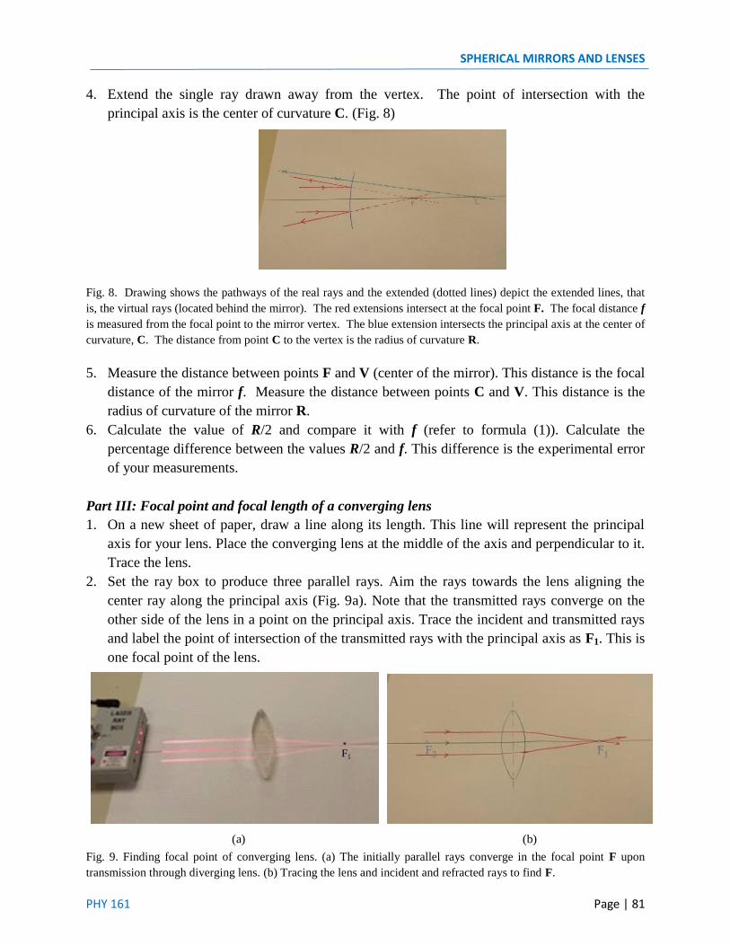
SPHERICAL MIRRORS AND LENSES
PHY 161 Page | 81
4. Extend the single ray drawn away from the vertex. The point of intersection with the
principal axis is the center of curvature C. (Fig. 8)
Fig. 8. Drawing shows the pathways of the real rays and the extended (dotted lines) depict the extended lines, that
is, the virtual rays (located behind the mirror). The red extensions intersect at the focal point F. The focal distance f
is measured from the focal point to the mirror vertex. The blue extension intersects the principal axis at the center of
curvature, C. The distance from point C to the vertex is the radius of curvature R.
5. Measure the distance between points F and V (center of the mirror). This distance is the focal
distance of the mirror f. Measure the distance between points C and V. This distance is the
radius of curvature of the mirror R.
6. Calculate the value of R/2 and compare it with f (refer to formula (1)). Calculate the
percentage difference between the values R/2 and f. This difference is the experimental error
of your measurements.
Part III: Focal point and focal length of a converging lens
1. On a new sheet of paper, draw a line along its length. This line will represent the principal
axis for your lens. Place the converging lens at the middle of the axis and perpendicular to it.
Trace the lens.
2. Set the ray box to produce three parallel rays. Aim the rays towards the lens aligning the
center ray along the principal axis (Fig. 9a). Note that the transmitted rays converge on the
other side of the lens in a point on the principal axis. Trace the incident and transmitted rays
and label the point of intersection of the transmitted rays with the principal axis as F1. This is
one focal point of the lens.
F1F1F2
(a) (b)
Fig. 9. Finding focal point of converging lens. (a) The initially parallel rays converge in the focal point F upon
transmission through diverging lens. (b) Tracing the lens and incident and refracted rays to find F.
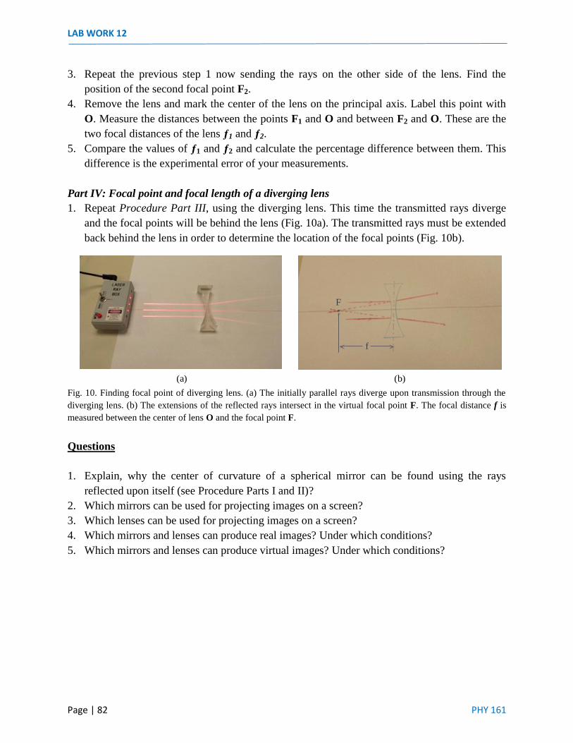
LAB WORK 12
Page | 82 PHY 161
3. Repeat the previous step 1 now sending the rays on the other side of the lens. Find the
position of the second focal point F2.
4. Remove the lens and mark the center of the lens on the principal axis. Label this point with
O. Measure the distances between the points F1 and O and between F2 and O. These are the
two focal distances of the lens ƒ1 and ƒ2.
5. Compare the values of ƒ1 and ƒ2 and calculate the percentage difference between them. This
difference is the experimental error of your measurements.
Part IV: Focal point and focal length of a diverging lens
1. Repeat Procedure Part III, using the diverging lens. This time the transmitted rays diverge
and the focal points will be behind the lens (Fig. 10a). The transmitted rays must be extended
back behind the lens in order to determine the location of the focal points (Fig. 10b).
Fig. 10. Finding focal point of diverging lens. (a) The initially parallel rays diverge upon transmission through the
diverging lens. (b) The extensions of the reflected rays intersect in the virtual focal point F. The focal distance f is
measured between the center of lens O and the focal point F.
Questions
1. Explain, why the center of curvature of a spherical mirror can be found using the rays
reflected upon itself (see Procedure Parts I and II)?
2. Which mirrors can be used for projecting images on a screen?
3. Which lenses can be used for projecting images on a screen?
4. Which mirrors and lenses can produce real images? Under which conditions?
5. Which mirrors and lenses can produce virtual images? Under which conditions?
(a) (b)
f
F

PHY 161 Page | 83
LAB
WORK 13
FORMATION OF IMAGES BY A CONVERGING LENS
Objective
The objective of this lab work is to study the principles of formation of images by converging
lenses.
Task 1: Determine focal length of a converging lens.
Task 2: Verify the formulae of magnification of a converging lens.
Task 3: Verify the Lens Equation.
Task 4: Find the range of object distances required for formation of real and virtual images.
Physical Principles
A converging lens, also known as a convex lens, is a lens capable of collecting initially parallel
light rays into one point upon they pass the lens. This point is known as the focal point F. The
distance between the focal point and the lens’ center is called the focal distance f. If a shiny
object is placed in front of a converging lens at a distance do from its center (object distance) so
that do > f, the rays emitted by the object and passing through the lens will converge and form an
image of the object, Fig. 1.
F
C
f
do di
Object
Image
Lens
Fig. 1. Real image formed by the rays passing through a converging lens. C – center of lens; F – focal point; f –
focal length; do – object distance; di – image distance.
This image formed by the real rays can be seen by projecting it on a screen. The distance di
between the image and the lens’ center is called the image distance. The formula connecting all
three distances do, di and f is known as the Lens Equation (1):
1
𝑑𝑜+
1
𝑑𝑖
=1
𝑓 . (1)

LAB WORK 13
Page | 84 PHY 161
If the object is placed at a distance shorter than the focal length do < f, all the rays emitted by the
object and passing through the lens will diverge and no real image will be formed. However, a
virtual image of the object will be formed. Since the virtual image is not formed by real light
rays, it cannot be projected on a screen. Yet it can be seen when looking at the object through the
lens.
The image, both real and virtual, is of the same shape as the object. However its size hi can be
very different from that of the size of object ho. The ratio hi/ho = m is known as magnification of
lens. There is a simple relation between the ratio di /do and magnification, m:
𝑚 =ℎ𝑖
ℎ𝑜= −
𝑑𝑖
𝑑𝑜 (2)
The magnitude and sign of the magnification m describe the size of the image and its orientation.
Upright images have positive magnification, while inverted images have negative magnification.
If the image is larger than object, the magnification is greater than 1, while for images smaller
than objects the magnification is less than 1.
In order to calculate magnification correctly using formula 2, you must know the sign convention
for the distances do, di and f (see Table 1 below).
Table 1. Sign Convention for Lenses
Parameter Sign Condition
Focal Length, f
+ For converging lenses
- For diverging lenses
Object Distance, do
+ If the object is in front of lens (real object)
- If the object is behind lens (virtual object)
Image Distance, di
+ If the image is behind lens
- If the image is in front of lens
Object Size, ho
+ Upright orientation
- Inverted orientation
Image Size, hi
+ Upright orientation
- Inverted orientation

FORMATION OF IMAGES BY A CONVERGING LENS
PHY 161 Page | 85
Formula (1) can also be presented as an equation:
y = -x + 1/f, (3)
where y = 1/di, x = 1/do. This equation, when plotted as a graph, reveals a linear dependence with
slope = -1. The line intercepts the axes at y0 = 1/f and x0 = 1/f (Fig. 2). Thus plotting the
dependence (3) for different do and di and finding the intersections with the axes, one can find
focal length of the lens:
f = 1/y0 = 1/x0. (4)
Fig. 2. Sample graph of inverse image distances versus inverse object distances (equation (3)). It is a linear
dependence with slope -1. The fitting line intersects both axes at values 1/f.
Apparatus
Vernier dynamics system track
Vernier light source
Vernier 20cm converging lens
Vernier Screen
Small white Ruler
LED lamp
Procedure and Calculations
1. Attach the light source assembly on the track (Fig. 3). Position it so that the pointer at the
base is at the 2 cm mark and the light source faces the other end of the track. Turn the light
source wheel until the number “4” is visible in the opening. This will be the “object” for this
experiment.
fxy
1
1/di vs 1/do
1/di
1/do
yf
1
xf
1
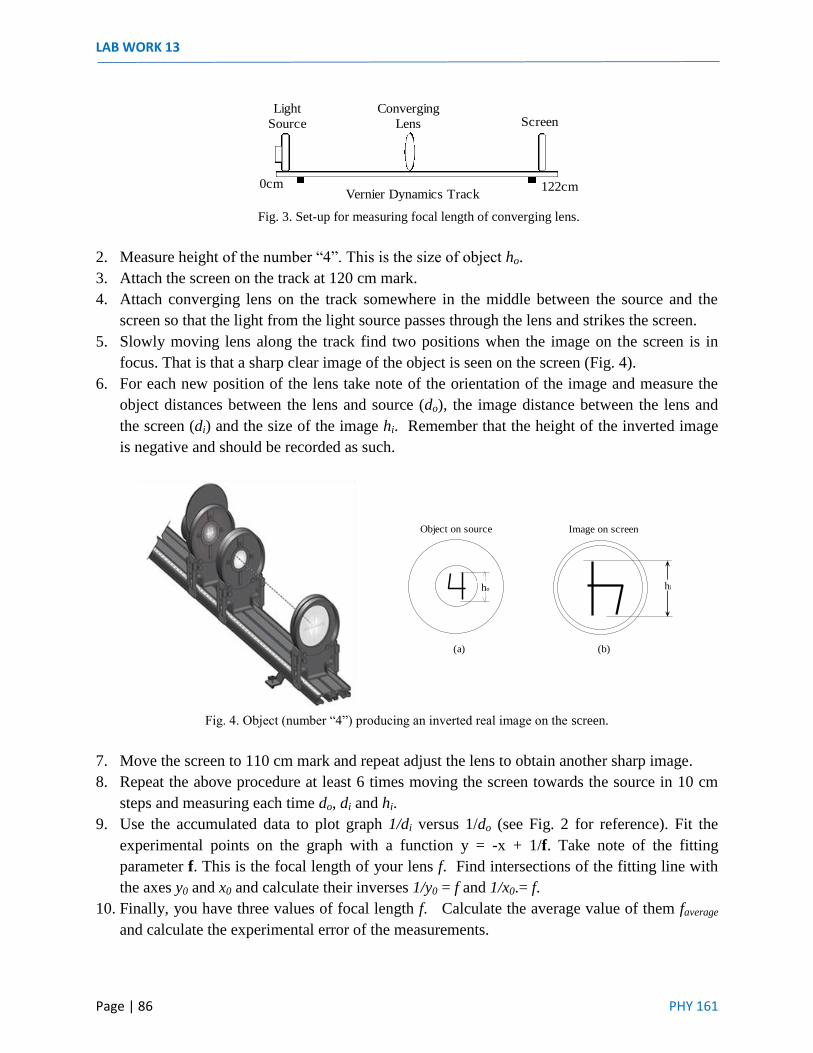
LAB WORK 13
Page | 86 PHY 161
Light
Source
Converging
Lens Screen
Vernier Dynamics Track0cm 122cm
Fig. 3. Set-up for measuring focal length of converging lens.
2. Measure height of the number “4”. This is the size of object ho.
3. Attach the screen on the track at 120 cm mark.
4. Attach converging lens on the track somewhere in the middle between the source and the
screen so that the light from the light source passes through the lens and strikes the screen.
5. Slowly moving lens along the track find two positions when the image on the screen is in
focus. That is that a sharp clear image of the object is seen on the screen (Fig. 4).
6. For each new position of the lens take note of the orientation of the image and measure the
object distances between the lens and source (do), the image distance between the lens and
the screen (di) and the size of the image hi. Remember that the height of the inverted image
is negative and should be recorded as such.
Fig. 4. Object (number “4”) producing an inverted real image on the screen.
7. Move the screen to 110 cm mark and repeat adjust the lens to obtain another sharp image.
8. Repeat the above procedure at least 6 times moving the screen towards the source in 10 cm
steps and measuring each time do, di and hi.
9. Use the accumulated data to plot graph 1/di versus 1/do (see Fig. 2 for reference). Fit the
experimental points on the graph with a function y = -x + 1/f. Take note of the fitting
parameter f. This is the focal length of your lens f. Find intersections of the fitting line with
the axes y0 and x0 and calculate their inverses 1/y0 = f and 1/x0.= f.
10. Finally, you have three values of focal length f. Calculate the average value of them faverage
and calculate the experimental error of the measurements.
Object on source Image on screen
hiho
(a) (b)

FORMATION OF IMAGES BY A CONVERGING LENS
PHY 161 Page | 87
11. For each pair of di and /do and corresponding hi and ho calculate magnification according to
formula (2) and find the percent difference between m = di/do and m = hi/ho. Calculate the
average of these differences. This is the experimental error of your measurements.
12. Verify the Lens Equation. For this, calculate the value 1/di + 1/do for each pair of di and /do
and compare it with the value of 1/faverage. Calculate the percent difference between the
values and calculate the average percent difference of them. This is the experimental error of
your measurements.
Questions
1. Could this experiment be constructed using a diverging lens? Explain you answer.
2. Using the value of f you have obtained, draw a ray diagram, to scale, for the first set of values
of do and di. Use three rays to construct the image.
3. Predict the shortest distance between the source and screen when it is still possible to obtain
sharp image.

LAB WORK 13
Page | 88 PHY 161

PHY 161 Page | 89
APPENDIX 1 PREPARING LABORATORY REPORTS
I. General Requirements
Preparation of laboratory reports is the most important work of a student participating in a laboratory class. Despite that students work in groups, reports must be written personally by each student. No plagiarized/copied reports -- full or in parts -- will be accepted. Although the content of a lab report considerably depends on the level of knowledge and creativity of a student, its structure should be well defined and consist of the following parts: 1. Title page – the first separate page showing the student name, course and section numbers,
experiment title, date of the performance of the experiment and the names of your laboratory partners.
2. Objectives - a short description (a few sentences) of the purpose and aim of the experiment. 3. Physical principles - a short description (up to one page) of the basic physical principles,
definitions and relevant formulae describing the experiment and used for the analysis of the obtained experimental data.
4. List of the experimental equipment used. 5. Experimental procedure - description and explanation of the major steps of performance of
the experiment. 6. Laboratory Data Sheet with the original experimental data preferentially arranged in tabular
form. IMPORTANT: The lab data sheet of every student must be signed by the instructor at the end of the lab work session. The lab report without a signed data sheet is not acceptable.
7. Data Analysis and Graphs. This part of the report contains computations of the physical values and their experimental errors with indication of the corresponding units. It is important that errors of measurements of the physical values are estimated and presented explicitly in each laboratory report. Standard graph paper or plotting software can be used for the graphical presentation of the experimental and calculated data.
8. Discussion. In this section, students discuss the obtained experimental data, results of calculations, graphs and the experimental errors. Discussion is the most creative and important part of the laboratory report. Quality of the Discussion largely determines the grade of the laboratory report.
9. Conclusion, in which a statement is made as to whether the aim of the laboratory work has been achieved. In most cases, this statement is supported by the numerical data obtained.
10. Answers to the Questions given at the end of every experiment write-up in your laboratory manual.

APPENDIX 1
Page | 90 PHY 161
II. Graphical Presentation of Data 1. Arrange the quantities to be plotted in tabular form. 2. Find out which of the quantities is the cause (independent variable) of the measured
dependence. This quantity is plotted along the x-axis. The other quantity (dependent variable) is plotted along the y-axis.
3. Choose the scale of units for each axis of the graph so that the plotted experimental points occupy most of the graph space.
4. Plot each experimental point by indicating its position by a dot. 5. Attach a legend to each axis which indicates what is plotted along that axis and, in addition,
mark the main divisions of each axis in units of the quantity being plotted. 6. Draw a smooth curve showing the distribution of the experimental points. This curve needs
not necessarily to pass exactly through each point, but should run close enough to the points in order to clearly show their distribution. Usually, a correctly drawn curve leaves on the average as many points on one side as it has on the other.
7. Label the graph. That is, include a title which indicates what dependence the graph presents. III. Errors of Measurements When performing physical experiments and taking measurements the encounter of errors is inevitable. However accurate the measuring instrument is and however accurate the experimentalist is, the results of the measurements cannot be absolutely precise. There are many reasons for this unavoidable inaccuracy, the major causes being the following: Blunders are the errors due to carelessness in performing measurement. This is the commonest and simplest type of error which can be relatively easily reduced, or even eliminated. Blunders are diminished by experience and the repetition of measurements. Personal Errors are these peculiar to a particular person performing measurements. For example, beginners very often try to fit measurement to some preconceived notion. Also, beginners are often prejudiced in favor of their first observations. Systematic Errors are errors associated with the particular instruments or technique of measurement being used. Suppose we have a book of a size 195 mm. This size is measured by laying a ruler against the book, with one end of the ruler at one edge of the book. If the first “0” mark on the ruler is not exactly at its end, but shifted by 1 mm, then the ruler is like to tell us that the book is 194 mm wide. Thus the measured value has 1 mm error. Since this error will appear every time when we use this ruler, this error is systematic specific of this very ruler. If a thermometer immersed in boiling pure water at normal pressure reads 102°C (must be 100°C), it is improperly calibrated. Thus, the systematic error of this thermometer is 2°C for the measurements of temperatures about 100°C.
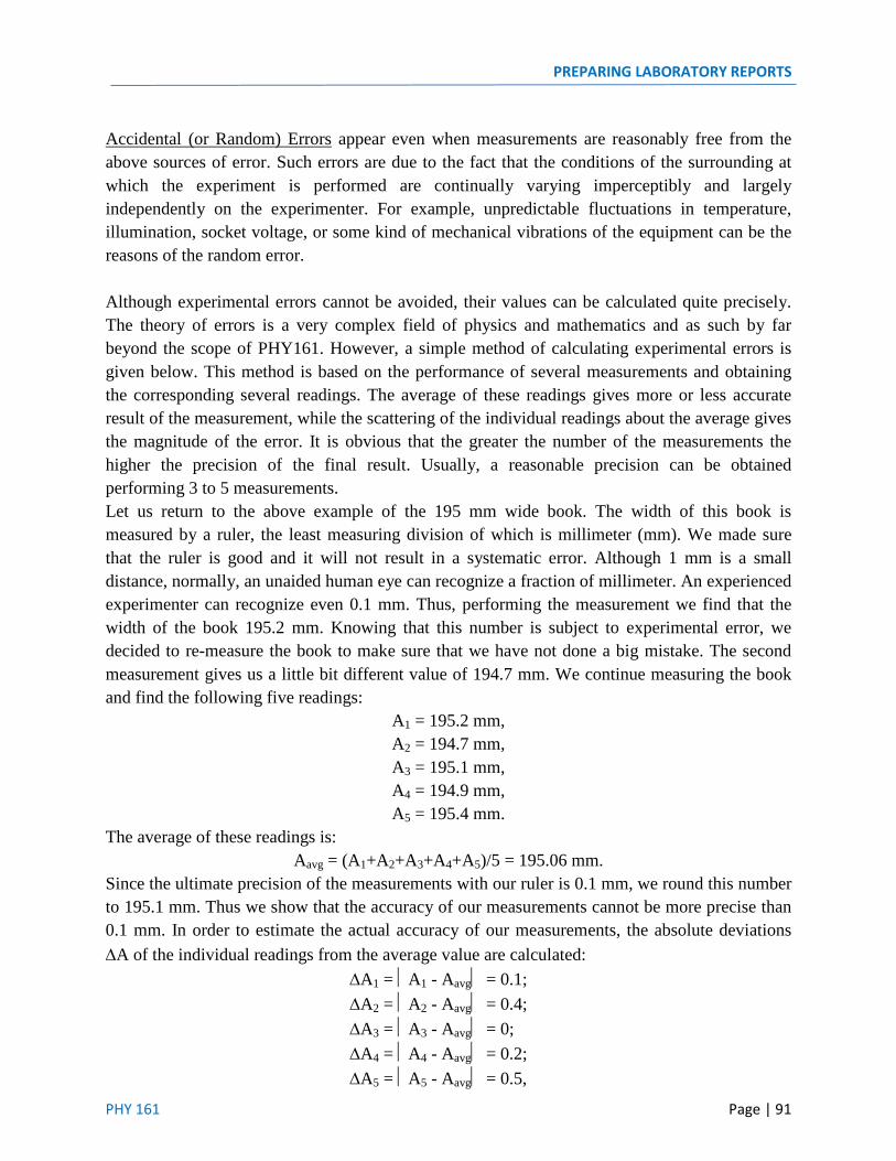
PREPARING LABORATORY REPORTS
PHY 161 Page | 91
Accidental (or Random) Errors appear even when measurements are reasonably free from the above sources of error. Such errors are due to the fact that the conditions of the surrounding at which the experiment is performed are continually varying imperceptibly and largely independently on the experimenter. For example, unpredictable fluctuations in temperature, illumination, socket voltage, or some kind of mechanical vibrations of the equipment can be the reasons of the random error. Although experimental errors cannot be avoided, their values can be calculated quite precisely. The theory of errors is a very complex field of physics and mathematics and as such by far beyond the scope of PHY161. However, a simple method of calculating experimental errors is given below. This method is based on the performance of several measurements and obtaining the corresponding several readings. The average of these readings gives more or less accurate result of the measurement, while the scattering of the individual readings about the average gives the magnitude of the error. It is obvious that the greater the number of the measurements the higher the precision of the final result. Usually, a reasonable precision can be obtained performing 3 to 5 measurements. Let us return to the above example of the 195 mm wide book. The width of this book is measured by a ruler, the least measuring division of which is millimeter (mm). We made sure that the ruler is good and it will not result in a systematic error. Although 1 mm is a small distance, normally, an unaided human eye can recognize a fraction of millimeter. An experienced experimenter can recognize even 0.1 mm. Thus, performing the measurement we find that the width of the book 195.2 mm. Knowing that this number is subject to experimental error, we decided to re-measure the book to make sure that we have not done a big mistake. The second measurement gives us a little bit different value of 194.7 mm. We continue measuring the book and find the following five readings:
A1 = 195.2 mm, A2 = 194.7 mm, A3 = 195.1 mm, A4 = 194.9 mm, A5 = 195.4 mm.
The average of these readings is: Aavg = (A1+A2+A3+A4+A5)/5 = 195.06 mm.
Since the ultimate precision of the measurements with our ruler is 0.1 mm, we round this number to 195.1 mm. Thus we show that the accuracy of our measurements cannot be more precise than 0.1 mm. In order to estimate the actual accuracy of our measurements, the absolute deviations ∆A of the individual readings from the average value are calculated:
∆A1 = A1 - Aavg = 0.1; ∆A2 = A2 - Aavg = 0.4; ∆A3 = A3 - Aavg = 0; ∆A4 = A4 - Aavg = 0.2; ∆A5 = A5 - Aavg = 0.5,
APPENDIX 1
Page | 92 PHY 161
The average of these deviations gives us an estimate of the actual accuracy of our measurements: ∆Aavg = (∆A1+∆A2+∆A3+∆A4+∆A5)/5 = 0.24 mm.
We round the obtained number to 0.2 mm and present the result of the measurements in the final form:
A = Aavg ± ∆Aavg = 195.1 ± 0.2 mm. This result indicates that we have measured the width of the book and found that it is 195.1 mm with accuracy (error of measurements) 0.2 mm. Percent Error (PE): Sometimes, it is more convenient to present the experimental error as a percentage of the measured value. Doing this we actually calculate so-called percent error
𝑃𝑃𝑃𝑃 = |𝐸𝐸𝐸𝐸𝐸𝐸𝐸𝐸𝐸𝐸 𝐸𝐸𝑜𝑜 𝑀𝑀𝑀𝑀𝑀𝑀𝑀𝑀𝑀𝑀𝐸𝐸𝑀𝑀𝑀𝑀𝑀𝑀𝑀𝑀𝑀𝑀𝑀𝑀|𝐴𝐴𝐴𝐴𝑀𝑀𝐸𝐸𝑀𝑀𝐴𝐴𝑀𝑀 𝑉𝑉𝑀𝑀𝑉𝑉𝑀𝑀𝑀𝑀
× 100%.
In the case of our example, that is the book we measured, the percent error of the measurements is (0.2/195.1)×100% = 0.1%. Percentage Difference (PD). In some laboratory works, you will measure the physical value which are well known, e.g. the magnetic permeability of free space µ0 = 1.25664×10⁻⁶ Tm/A. This well known value has been obtained by highly experienced scientists through many measurements with very precise research instruments. Thus we believe, that the value 1.25664×10⁻⁶ Tm/A is a very accurate one for µ0 and we term it “standard value”. You have to compare the result of your measurements with this standard value and calculate the difference between them. This difference presented as percent of the standard value (percentage difference) gives you an impression about the accuracy of your measurements. The percent difference is computed as follows:
𝑃𝑃𝑃𝑃 =|𝑆𝑆𝑆𝑆𝑆𝑆𝑆𝑆𝑆𝑆𝑆𝑆𝑆𝑆𝑆𝑆 𝑉𝑉𝑆𝑆𝑉𝑉𝑉𝑉𝑉𝑉 − 𝑃𝑃𝐸𝐸𝐸𝐸𝑉𝑉𝑆𝑆𝐸𝐸𝐸𝐸𝑉𝑉𝑆𝑆𝑆𝑆𝑆𝑆𝑉𝑉 𝑉𝑉𝑆𝑆𝑉𝑉𝑉𝑉𝑉𝑉|
𝑆𝑆𝑆𝑆𝑆𝑆𝑆𝑆𝑆𝑆𝑆𝑆𝑆𝑆𝑆𝑆 𝑉𝑉𝑆𝑆𝑉𝑉𝑉𝑉𝑉𝑉× 100%
IV. Additional Instructions 1. Each section of the laboratory report must be clearly labeled. 2. Reports must be typed on standard paper. One-side typing only! Hand-written reports are
not acceptable! 3. Ruler and compass should be used for diagrams. No hand drawings are accepted! 4. All pages of the lab report including the laboratory data sheet must be numbered and stapled
together. 5. Be as neat as possible in order to facilitate reading your report. 6. Laboratory reports are due one week following the experiment. No reports will be accepted
after the "Due-date" without penalty as determined by the instructor. 7. No student can pass the PHY 161 course unless he or she has submitted the complete set of
laboratory reports.

PHY 161 Page | 93
APPENDIX 2
SAMPLE LABORATORY REPORT
MAGNETIC FIELD OF A LONG STRAIGHT WIRE
Course PHY161
Section 08260
Student Name: Paul Getty, Jr.
Lab Partner: Ann Taylor, Esq.
Lab work date 11. 07. 2014

APPENDIX 2
Page | 94 PHY 161
Objectives
The objective of this lab work was to study distribution and strength of magnetic field created by
a long straight wire carrying DC current. In particular, we were to verify that the strength of
magnetic field around straight wire is proportional to the current in the wire and inversely
proportional to the distance from the wire. We also were to measure experimentally the magnetic
permeability of free space µ0.
Physical Principles
When electric current flows in a straight wire, a magnetic field is created around this wire
encircling it like concentric circles. The strength of this field B depends on the magnitude of
current I and the distance from the wire r and it is given by the formula:
𝐵 =µ0𝐼
2𝜋𝑟 ,
where µ0= 1.2610-6
T*m/A = 0.00126 mT*m/A is the magnetic permeability of free space. This
formula shows that the magnetic field strength is proportional to the current in the wire and
inversely proportional to the distance from the wire.
Apparatus used in this experiment
- Power supply
- One long aluminum pole
- Three short aluminum poles
- One table clamp
- Three right angle clamps
- One small rod clamp
- A piece of long straight insulated
- Ammeter
- Vernier LabPro interface and magnetic field sensor
Procedure
1. Preparation of the experimental setup
We assembled the experimental setup as instructed. In fig. 1 below the layout of the setup is
shown.
1

SAMPLE LABORATORY REPORT
PHY 161 Page | 95
Fig. 1. Experiment set-up
Particular attention was paid to the correct position of the wire, which must be stretched strictly
vertically with respect to the working table. Then we connected the Vernier Magnetic Field
Sensor to the Vernier LabPro Interface and set the switch on the sensor to position “High”. After
that we connected the LabPro interface to the computer using an USB cable. Finally, we
prepared the computer for data collection by opening Logger Pro. We made sure that on the
graph, which appeared on the screen, the vertical axis was labeled “Magnetic Field” and the utits
were “milliTesla” [mT]. Correspondingly, the horizontal axis was labeled “Time” and the units
were “seconds” [s].
Once the setup had been assembled and prepared for the work, we asked our technician to do the
final check before we switched on the power supply.
2. Measuring the dependence of magnetic field strength versus current
We placed the magnetic field sensor at a distance of 3 cm from the wire. Then we switched on
the power supply and set the current at 4 A. Slowly rotating the magnetic field sensor we found
its position for the maximum positive reading. After that tuning, we made sure that the sensor
was fixed properly and did not change its position during the whole experiment. Once all those
adjustments had been done we switched off the power supply and set current to 0 A. After that,
with no current flowing through the wire, we “zeroed” the sensor in order to subtract the
contribution of the Earth’s magnetic field from the reading of the sensor.
When the sensor had been zeroed, we clicked on the “collect” icon and turned on the power
supply. Now the sensor measured the magnetic field created by the current in the wire. We
changed the current from 0.5 A to 5 A in steps of about 0.5 A every time taking exact reading of
the ammeter, reading of the sensor and entering the obtained values in the columns “Current”
and “BField” correspondingly (Table I below). When the measurements were finished and the
data collected, we clicked the icon “stop” and switched off the power supply.
We plotted the graph "Magnetic Field" versus "Current" and fitted the experimental points with a
straight line function y = (m/(2*pi*0.03))*x. Among the parameters of the fitting function, we
found the parameter m1, which is the magnetic constant µ0. So we expected m to be close to the
value 0.00126 mT*m/A.
2

APPENDIX 2
Page | 96 PHY 161
3. Measuring the dependence of magnetic field strength versus the distance from the wire
We set the current in the wire 4 A and adjusted the magnetic field sensor in the way we did it in
the previous experiment. On the computer screen, we opened a new graph window. After that,
we moved the sensor to a distance of 1 cm from the wire and slowly rotating it about its axis we
found the maximum reading. Then we switched off current and, with no current flowing through
the wire, we "zeroed" the sensor again. Once the zeroing had been done we switched on current,
set it again at 4 A, took the sensor reading and enter the obtained data in the columns “Distance”
and "BField" correspongdingly (Table II below). We repeated this procedure for the distances
from 2.5 to 7 cm in 0.5 cm steps. The distances were measured between the wire center and the
sensor center with a ruler with precision of 1 mm.
Once the graph with the experimental points had been formed, we fitted the experimental data
with the function y = (4*m/2*pi)/x and took note of the fitting parameter m, which was the
magnetic constant µ0. So we expected m to be close to the value 0.00126 mT*m/A.
Calculations
The numerical results of our measurements are presented in tables below:
Table I Table II
BField vs I BField vs D
Current, I
[A]
BField
[mT]
Distance, D
[m]
BField
[mT]
0.500 0.004822 0.025 0.034204
1.077 0.009375 0.030 0.026550
1.486 0.011743 0.035 0.021399
2.072 0.016711 0.040 0.018262
2.554 0.020825 0.045 0.017969
3.038 0.025659 0.050 0.015405
3.550 0.029431 0.055 0.014868
4.000 0.033545 0.060 0.014905
4.500 0.038037 0.065 0.013000
5.027 0.043250
3

SAMPLE LABORATORY REPORT
PHY 161 Page | 97
The result of procedure 2 is the graph below (Fig. 2):
Fig. 2. Dependence of strength of magnetic field on current flowing on a straight wire. The experimental
data is fitted with a straight line. The fitting parameter m = 0.001322 mT*m/A.
We found the value of the fitting parameter m = 0.001322 mT*m/A. This is our first calculated
value of µ0. The percentage difference between the rated value of µ0 = 0.00126 mT*m/A and the
measured value m = 0.001322 mT*m/A is:
100% × 0.001322 – 0.00126/0.00126 ≈ 4.9%
The result of procedure 3 is the graph below (Fig. 3)
Fig. 3. Dependence of strength of magnetic field on the radial distance from the wire. The experimental
data are fitted with a hyperbolic function with the fitting parameter m = 0.001266 mT*m/A.
4

APPENDIX 2
Page | 98 PHY 161
We found m = 0.001266 mTm/A. This is our second calculated value of µ0. The percentage
difference between the rated value of µ0 = 0.00126 mT*m/A and the measured value 0.001266
mT*m/A is:
100% × 0.001266 – 0.00126/0.00126 ≈ 0.5%
Discussion
The measurement of the dependence of magnetic field strength B versus current I has been
performed for currents from 0.5 A to 5 A. With the steps of 0.5 A, we obtained 10 experimental
points. Our data is presented on the attached graph. We know that theoretically this dependence
is a linear function passing through the origin, that is a dependence of the type B = A1I. Thus the
magnetic field strength increases proportionally with current. We fitted the experimental data
with the linear function shown above. The fitting parameter m of this function corresponds to µ0.
It is seen that the fitting line is pretty close to the experimental points suggesting that we had a
good accuracy of our measurements. According to the formula for magnetic field shown in the
“Physical Principles” section, the slope of this dependence A1 = µ0/(2πr). We found the
magnitude of the fitting parameter m = 0.001322 mT*m/A. This gives us the first experimental
value µ0 = 1.3210-6
T*m/A. This is very close to the known value µ0 = 1.2610-6
T/A. The
percentage difference between these two values is reasonably low: only 4.9%. This low
difference confirms that our measurements were accurate.
The dependence of magnetic field B versus distance r from the wire has been measured for the
distance range from 2.5 cm to 6cm. We changed the distance in steps of 0.5cm and thus obtained
9 experimental points. According to the formula for the magnetic field created by long straight
current, it must be an inversely proportional dependence of a type B = A2/r. Indeed, it is clearly
seen that the greater the distance the weaker the magnetic field. We fitted the experimental points
with a hyperbolic function y = A2/x and found the value of the fitting parameter m = 0.001266
mT*m/A. Now the fitting curve is not this close to the experimental points as we had it in the
first experiment. Surprisingly, the fitting parameter m, which corresponds to µ0, appeares to be
very close to the standard value. Thus, we obtained the second experimental value µ0 =
1.26610-6
T/A, which is not very close to the known value µ0 = 1.2610-6
T/A. The percentage
difference between these two values is 0.5%.
A good accuracy of the measurements in the first experiment and even better in the second one
show that overall the experiment was successful. Yet we have some concern about our data
obtained in the second procedure. In that case the experimental points quite deviate from the
fitting curve. That was probably because of the different accuracy of the measurement of current
and distance. Indeed, in the first experiment, once the magnetic sensor was placed for the
measurements, it was not moved any more. The only variable was the magnitude of current,
which was set very accurately using a digital ammeter. In the second experiment, the magnetic
sensor was moved and adjusted every time. Thus this procedure allowed much more room for
experimental error. Besides, the size of the sensor was rather large and it was challenging to
measure accurately the distances between the sensor center and the wire with plain ruler.
5
SAMPLE LABORATORY REPORT
PHY 161 Page | 99
Conclusion
We believe that the objectives of the lab work were achieved. We have confirmed that the
strength of magnetic field created by long straight wire is proportional to the current flowing in it
and inversely proportional to the distance from the wire. We experimentally measured the
magnetic permeability of free space in two experiments and have found a good coincidence with
the known value of 1.2610-6
T*m/A. In one experiment we have obtained 1.3210-6
T*m/A
(experimental error of 5%) and in another experimenta we obtained 1.2710-6
T*m/A
(experimental error 0.5%).
Questions
1. Explain when the wire used in this experiment can be regarded as “long wire”.
Answer: The formula of the magnetic field shown in “Physical Principles” is strict only for
infinitely long wire. Any real wire has a limited length. However, the magnetic field created at
distances much shorter than the length of wire is described by this formula with a good precision.
2. What is the shape of magnetic field lines created by long straight wire with current?
Answer: The magnetic field lines are concentric circles with the wire passing through the center.
These circles are in the planes perpendicular to the wire.
3. The formula of the magnetic field strength implies that with the distance approaching zero
the field strength increases to infinity. Why the magnetic field is not infinitely high at the wire
sirface, where the distance from the wire seems to be zero?
Answer: The distance from the wire means the distance from its center. Since any real wire has a
certain diameter, even at the wire surface the distance is not zero and, consequently, the magnetic
field is not infinitely strong.
6

APPENDIX 2
Page | 100 PHY 161
7

SAMPLE LABORATORY REPORT
PHY 161 Page | 101
8

APPENDIX 2
Page | 102 PHY 161

PHY 161 Page | 103
APPENDIX 3 GRAPHICAL ANALYSIS 3.41
• PLOTTING YOUR DATA POINTS AND FINDING THE BEST FIT 1. Click on the GA 3.4 icon 2. The Graphical Analysis screen will be displayed:
3. On the Data Set Table with X and Y columns
click on either column to start entering your data. Use either the arrow keys or the mouse to move to the next cell.
4. As you enter data you will notice a graph will
develop as the data is plotted. Just continue entering your data till you are finished.
5. To delete the line that is connecting the points
either double click on the graph window. Select the Graph Options tab.
1 Adapted from Vernier Software & Technology – Graphical Analysis User’s Manual

APPENDIX 3
Page | 104 PHY 161
Click on Connect Lines to delete the original line on your graph. To add a title, click on the Title window. This window also gives the option to add a legend to your graph or change the grid style.
6. Finding the Best Linear Fit for
your graph: On the graph window click and drag the mouse across the segment of interest. The shaded area marks the beginning and end of the range. You may also select the segment of interest on your data columns and then clicking on the graph window to activate it.
7. With the graph window activated, select the Regression option either by clicking the
Linear Fit icon, on the toolbar or by selecting it from the Analyze Menu. To remove the regression line click the box in the upper corner of the helper object. The Linear Fit function fits the line y = m*x + b to the selected region of a graph and reports the slope (m) and y-intercept (b) coefficients. If more than one column or data set is plotted, a selection dialog will open for you to which set you want to fit. You may select more than one column for regression; in this case, a separate fit line will be applied to each graphed column.
As aforementioned, you can fit a line either to the whole graph or to a region of interest. Drag the mouse across the desired part of the graph to select it. Black brackets mark the beginning and end of the range.

BASIC PLOTTING WITH GRAPHICAL ANALYSIS
PHY 161 Page|105
8. If you wish to graph a fit other than y=mx+b, such as proportional, quadratic, cubic, exponential, etc, click on the Curve Fit icon from the toolbar. A Curve Fit dialog window will pop-up:
Select the function you wish to use. Click Try Fit. Then click OK.
9. To change the labels of your X and Y axes and include their respective units click on the column you wish to change and the dialog window below will pop-up:
On this dialog window, you will be allowed to give your column a name other than the default name. You may also include units such as m/s, cm/s2, etc. The drop down arrows allows you to enter a symbol, subscript or superscript.

APPENDIX 3
Page | 106 PHY 161
10. To change the scaling of your graph, right click on the desired graph and select autoscale or autoscale from zero. To modify manually, click on the highest or lowest number of the axis you wish to change and enter the new number, press Enter.
11. Select the orientation of your page. This is done by using Page Setup under the File
menu.
12. To print the entire screen select Print from the File menu or click the icon on
the toolbar. A dialog window will pop-up allowing you to enter your name or any comments you wish to add.
13. If you wish to print just the graph select it first and then go to the File menu and select
Print Graph… You may also print data table alone by selecting Print Data Table. For more information go to: http://www2.vernier.com/manuals/ga3manual.pdf Note that these basic graphing instructions can also be applied to LoggerPro.

PHY 161 Page | 107
APPENDIX 4
TECHNICAL NOTES ON VERNIER LABQUEST2 INTERFACE1
Once the LabQuest interface is connected to AC power or the battery has been charged, press the
power button located on the top of the unit, near the left edge. LabQuest will complete its
booting procedure and automatically launch the LabQuest App by default, as shown below. If the
screen momentarily shows a charge battery icon or does not light after a moment when used on
battery power, connect the power adapter to LabQuest and to an AC power source, then try the
power button again.
Power Button
Power on – If the screen is off for any reason (LabQuest is off, asleep, or the screen has
turned off to conserve battery power), press and release the power button to turn LabQuest
back on. If LabQuest was off, LabQuest will also complete its booting procedure that takes
about a minute and then display LabQuest App.
Sleep/wake – When LabQuest is on, press and release the power button once to put
LabQuest into a sleep mode. Note that the sleep mode does not start until you release the
power button. In this mode, LabQuest uses less power but the battery can still drain. This
mode is useful if you are going to return to data collection again soon, in which case waking
LabQuest from sleep is quicker than restarting after shutdown. To wake LabQuest from
sleep, press and release the power button. A LabQuest that is left asleep for one week will
automatically shutdown.
Shut down – To shut down LabQuest, hold the power button down for about five seconds.
LabQuest displays a message indicating it is shutting down. Release the power button, and
allow LabQuest to shut down. To cancel the shutdown procedure at this point, tap Cancel.
You can also shut down LabQuest from the Home screen. To do this, tap System and then
tap Shut Down.
Emergency shutdown – If you hold the power button down for about eight seconds, while it
is running. This is not recommended unless LabQuest is frozen, as you may lose your data
and potentially cause file system corruption.
1 Adapted from Vernier Software & Technology LabQuest2 User’s Manual.
Fig. 1 - LabQuest2 Interface

APPENDIX 4
Page | 108 PHY 161
Touch Screen
LabQuest has an LED backlit resistive touch screen that quickly responds to pressure exerted on
the screen. LabQuest is controlled primarily by touching the screen. The software is designed to
be finger-friendly. In some situations, you may desire more control for precise navigation. In
such cases, we recommend using the included stylus.
If you are having trouble viewing the color screen or are using LabQuest outside in bright
sunlight, we recommend changing to the High Contrast mode. Tap Preferences on the Home
screen, then tap Light & Power. Select the check box for High Contrast to enable this mode.
Hardware Keys
In addition to using the touch screen, the three hardware keys can also be used to control your
LabQuest.
Collect – Start and stop data collection within LabQuest App
Home – Launch the Home screen to access other applications
Escape – Close most applications, menus, and exit dialog boxes without taking action (i.e.,
cancel dialog boxes)
Sensor Ports
LabQuest has three analog sensor ports (CH 1, CH 2, and CH 3) for analog sensors such as our
pH Sensor, Temperature Probe, and Force Sensor. Also included is a full-size USB port for USB
sensors, USB flash drives, and USB printers. In addition to the power button, the top edge of
LabQuest has two digital sensor ports (DIG 1 and DIG 2) for Motion Detectors, Drop Counters,
and other digital sensors.
Fig. 2 - LabQuest2 Control Buttons

TECHNICAL NOTES ON VERNIER LABQUEST2 INTERFACE
PHY 161 Page|109
Audio ports are also located adjacent to the digital ports, as well as a microSD card slot for
expanding disk storage. On the side opposite of the analog ports, there is a stylus storage slot, an
AC power port for recharging the battery, and a mini USB port for connecting LabQuest to a
computer. In between these ports, there is a serial connection for charging the unit in a LabQuest
Charging Station.
For more information on the LabQuest2 interface please go to:
http://www2.vernier.com/manuals/labquest2_user_manual.pdf
Fig. 3- LabQuest2 Sensor Ports
Fig. 4 - LabQuest2 Additional Ports

APPENDIX 4
Page | 110 PHY 161
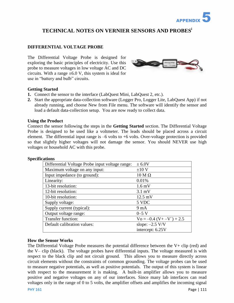
PHY 161 Page | 111
APPENDIX 5
TECHNICAL NOTES ON VERNIER SENSORS AND PROBESi
DIFFERENTIAL VOLTAGE PROBE
The Differential Voltage Probe is designed for
exploring the basic principles of electricity. Use this
probe to measure voltages in low voltage AC and DC
circuits. With a range ±6.0 V, this system is ideal for
use in “battery and bulb” circuits.
Getting Started
1. Connect the sensor to the interface (LabQuest Mini, LabQuest 2, etc.).
2. Start the appropriate data-collection software (Logger Pro, Logger Lite, LabQuest App) if not
already running, and choose New from File menu. The software will identify the sensor and
load a default data-collection setup. You are now ready to collect data.
Using the Product Connect the sensor following the steps in the Getting Started section. The Differential Voltage
Probe is designed to be used like a voltmeter. The leads should be placed across a circuit
element. The differential input range is –6 volts to +6 volts. Over-voltage protection is provided
so that slightly higher voltages will not damage the sensor. You should NEVER use high
voltages or household AC with this probe.
Specifications
Differential Voltage Probe input voltage range: ± 6.0V
Maximum voltage on any input: ±10 V
Input impedance (to ground): 10 M Ω
Linearity: 0.01%
13-bit resolution: 1.6 mV
12-bit resolution: 3.1 mV
10-bit resolution: 12.5 mV
Supply voltage: 5 VDC
Supply current (typical): 9 mA
Output voltage range: 0–5 V
Transfer function: Vo = –0.4 (V+ –V–) + 2.5
Default calibration values: slope: –2.5 V/V
intercept: 6.25V
How the Sensor Works The Differential Voltage Probe measures the potential difference between the V+ clip (red) and
the V– clip (black). The voltage probes have differential inputs. The voltage measured is with
respect to the black clip and not circuit ground. This allows you to measure directly across
circuit elements without the constraints of common grounding. The voltage probes can be used
to measure negative potentials, as well as positive potentials. The output of this system is linear
with respect to the measurement it is making. A built-in amplifier allows you to measure
positive and negative voltages on any of our interfaces. Since many lab interfaces can read
voltages only in the range of 0 to 5 volts, the amplifier offsets and amplifies the incoming signal
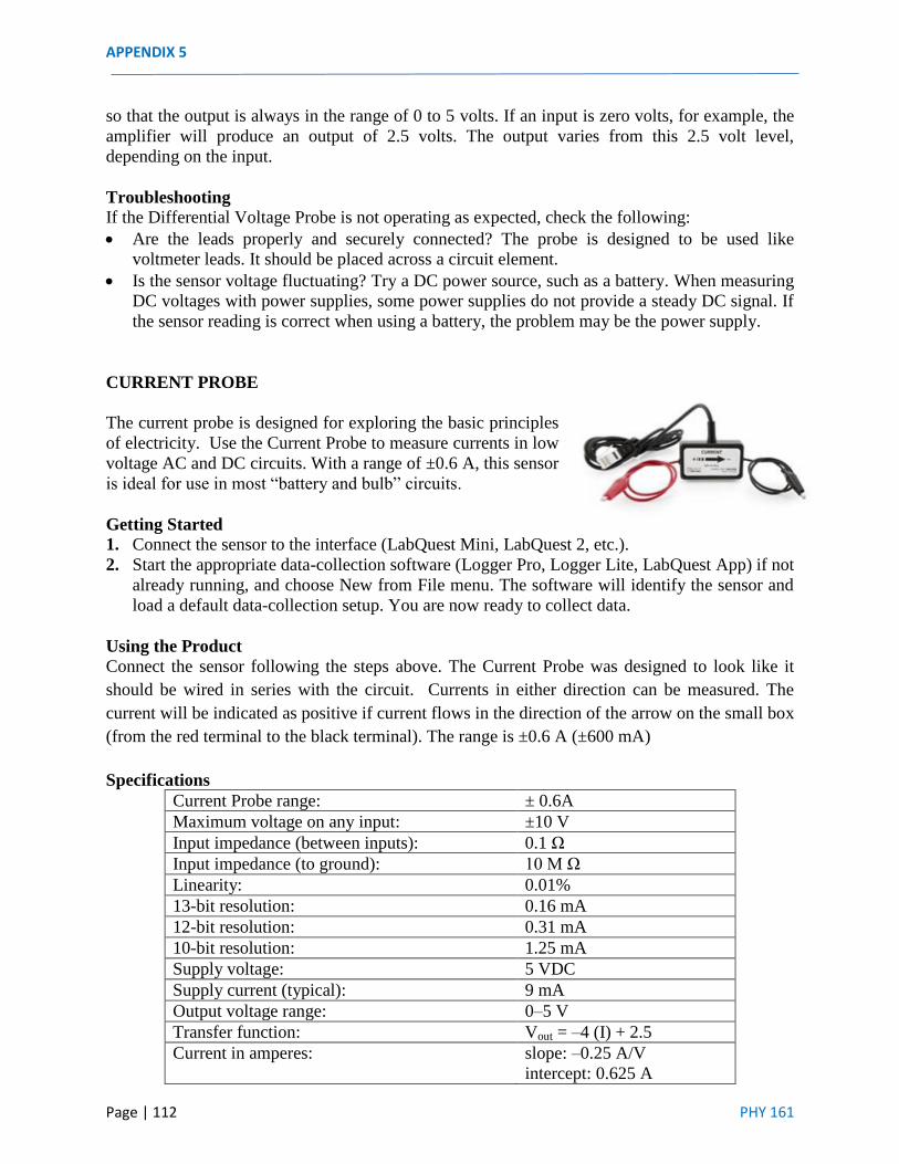
APPENDIX 5
Page | 112 PHY 161
so that the output is always in the range of 0 to 5 volts. If an input is zero volts, for example, the
amplifier will produce an output of 2.5 volts. The output varies from this 2.5 volt level,
depending on the input.
Troubleshooting If the Differential Voltage Probe is not operating as expected, check the following:
Are the leads properly and securely connected? The probe is designed to be used like
voltmeter leads. It should be placed across a circuit element.
Is the sensor voltage fluctuating? Try a DC power source, such as a battery. When measuring
DC voltages with power supplies, some power supplies do not provide a steady DC signal. If
the sensor reading is correct when using a battery, the problem may be the power supply.
CURRENT PROBE
The current probe is designed for exploring the basic principles
of electricity. Use the Current Probe to measure currents in low
voltage AC and DC circuits. With a range of ±0.6 A, this sensor
is ideal for use in most “battery and bulb” circuits.
Getting Started 1. Connect the sensor to the interface (LabQuest Mini, LabQuest 2, etc.).
2. Start the appropriate data-collection software (Logger Pro, Logger Lite, LabQuest App) if not
already running, and choose New from File menu. The software will identify the sensor and
load a default data-collection setup. You are now ready to collect data.
Using the Product
Connect the sensor following the steps above. The Current Probe was designed to look like it
should be wired in series with the circuit. Currents in either direction can be measured. The
current will be indicated as positive if current flows in the direction of the arrow on the small box
(from the red terminal to the black terminal). The range is ±0.6 A (±600 mA)
Specifications
Current Probe range: ± 0.6A
Maximum voltage on any input: ±10 V
Input impedance (between inputs): 0.1 Ω
Input impedance (to ground): 10 M Ω
Linearity: 0.01%
13-bit resolution: 0.16 mA
12-bit resolution: 0.31 mA
10-bit resolution: 1.25 mA
Supply voltage: 5 VDC
Supply current (typical): 9 mA
Output voltage range: 0–5 V
Transfer function: Vout = –4 (I) + 2.5
Current in amperes: slope: –0.25 A/V
intercept: 0.625 A

TECHNICAL NOTES ON VERNIER SENSORS AND PROBES
PHY 161 Page|113
Troubleshooting If the Current Probe is not operating as expected, plug the probe into an interface and run the
data-collection program. Use wire leads to connect the probe to a DC 2 power supply in series
with a known resistance. Use a voltage probe or voltmeter to measure the voltage of the supply.
Compare the measured current against the current calculated from Ohm’s law. Note: We
recommend a battery for this test, since some DC power supplies may not deliver clean DC
voltage.
MAGNETIC FIELD SENSOR
The Vernier Magnetic Field Sensor measures a
vector component of the magnetic field near
the sensor tip. The tip can be adjusted,
allowing the user to measure fields that are
parallel or perpendicular to the long axis of the
sensor. The Magnetic Field Sensor can be
used for a variety of interesting experiments
involving magnetic fields.
Measure and study the Earth’s magnetic field.
Determine the direction of magnetic north.
Study the magnetic field near a permanent magnet.
Measure the field near a current-carrying wire.
Measure the field at the opening of a solenoid.
Getting Started
1. Connect the sensor to the interface (LabQuest Mini, LabQuest 2, etc.).
2. Start the appropriate data-collection software (Logger Pro, Logger Lite, LabQuest App) if not
already running, and choose New from File menu. The software will identify the sensor and
load a default data-collection setup. You are now ready to collect data.
Using the Sensor Connect the sensor following the steps in the Getting Started section of this user manual. Use the
switch on the sensor shaft to select an appropriate range.
The 6.4 mT range is used to measure relatively strong magnetic fields around permanent
magnets and electromagnets.
The 0.32 mT range is used mainly to measure the magnetic field of the Earth and very weak
fields. It can be used for other magnets, but the sensor must remain in one position so that the
reading is not affected by the background field of the Earth.
Specifications
13-bit resolution: ±0.32 mT range: 0.0001 mT
±6.4 mT range: 0.002 mT
12-bit resolution: ±0.32 mT range: 0.0002 mT
±6.4 mT range: 0.004 mT
10-bit resolution: ±0.32 mT range: 0.0008 mT
±6.4 mT range: 0.016 mT

APPENDIX 5
Page | 114 PHY 161
Stored calibration value
(±0.32 mT range in millitesla)
slope: 0.160 mT/V
intercept: –0.320 mT
Stored calibration value
(±6.4 mT range in millitesla)
slope: 3.225 mT/V
intercept: –8.063 mT
Stored calibration value
(±0.32 mT range in gauss)
slope: 1.6 gauss/V
intercept: –3.2 gauss
Stored calibration value
(±6.4 mT range in gauss)
slope: 32.25 gauss/V
intercept: –80.625 gauss
How the Sensor Works The sensor uses a Hall-effect transducer. It produces a voltage that is linear with magnetic field.
The sensor measures the component of the magnetic field that is perpendicular to the white dot
on the end of the sensor tip. The reading is positive when the white dot on the sensor points
toward a magnetic south pole.
The switch on the sensor shaft is used to select the range. On the 6.4 mT range, each
volt measured by the transducer represents 32 gauss (3.2 × 10⁻³
tesla). The range of
the sensor is ±64 gauss or ±6.4 × 10⁻³
tesla. On the 0.3 mT range, each volt
measured represents 1.6 gauss (1.6 × 10⁻⁴
tesla). The range of the sensor is ±3.2
gauss or ±3.2 × 10⁻⁴
tesla.
If the sensor tube is held vertically with the tip horizontal, and rotated
until the maximum voltage is found, the tip with the white dot will point to
magnetic north. The magnetic inclination in your area can be found by holding the
tube so that the white dot is facing north, and rotating the sensor end of the tube
down until the voltage reaches a maximum. The angle of the tip from the vertical
position is the magnetic inclination. Note that the north pole of a freely suspended
magnet points north, since the magnetic pole of the Earth in the northern
hemisphere is a south magnetic pole.
Troubleshooting If you are getting unexpected or unusual readings from the Magnetic Field Sensor, first confirm
that the range setting is appropriate for the experiment. The ±6.4 mT range is used to measure
relatively strong magnetic fields around permanent magnets and electromagnets; the ±0.32 mT
range is used to measure the magnetic field of the Earth and very weak fields. If you are using
the ±0.32 mT range for investigating permanent magnets, make sure that the sensor remains in
one position so that the reading is not affected by the background field of the Earth.
i The information provided here was taken from Vernier Software & Technology’s User Manuals for the respective probes and sensors used in this manual. For more information go to www.vernier.com

PHY 161 Page | 115
APPENDIX 6 MULTIMETERS AND POWER SUPPLIES
DIGITAL MULTIMETER A digital multimeter (DMM) is a test tool used to measure two or more electrical values—principally voltage (volts), current (amps) and resistance (ohms). It is a standard diagnostic tool for technicians in the electrical/electronic industries1
.
Fig. 1 – Fluke Multimeter Dial Settings
To perform measurements required in experiments in this manual set the dial to the desire mode • To measure DC ( ) Voltage set the dial to the proper setting (Fig. 1). This setting will be
used for experiments such as Equipotentials and Electric Field Lines, Ohm’s Law, Kirchhoff’s Rules, Direct Current Meters and Sources of EMF. The probes or wires must be connected as shown on Fig. 2a.
• To measure AC (~) Voltage set the dial to the proper setting as shown on Fig. 1. This setting will be used in AC Circuits exp. The probes or wires must be connected as shown on Fig. 2a.
• To measure DC ( ) Millivolts set the dial to the proper setting as shown on Fig. 1. This setting will be used in the Resistivity experiment where voltage readings are below 1V.
• To measure Resistance (Ω) set dial to the prop er setting as shown on Fig. 1 and connect probes as shown on Fig. 2a. To measure Capacitance ( ) keep the dial on the same setting but press the shift key to get readings in µF or nF. This setting will be used for experiments such as Kirchhoff’s Rules, Connection of Resistors and Capacitors in Series and Parallel, RC Circuits, AC Circuits.
• To measure small DC ( ) Current (mA) (current 0-400mA) set the dial to the proper setting as shown on Fig. 1. Press the shift key to obtain DC readings. This setting will be used for experiments such as Ohm’s Law, Resistivity, Kirchhoff’s Rules, Direct Current Meters and Sources of EMF. The probes or connecting wires must be connected as shown on Fig. 2b.
• To measure small AC (~) Current (mA) set the dial to the proper setting as shown on Fig. 1. This setting will be used in AC Circuits experiment. The probes or connecting wires must be connected as shown on Fig. 2b. Note that this setting is used for current ranges from 0 to 400mA.
1 Definition from Fluke Multimeter User’s Manual.

APPENDIX 6
Page | 116 PHY 161
• To measure large DC ( ) Current (A) with current ranges 0-10 A set the dial to the proper setting as shown on Fig. 1 and press the shift key to obtain DC readings. This setting will be used for the Magnetic Field in a Slinky Solenoid experiment. The probes or connecting wires must be connected as shown on Fig. 2b.
Fig. 2 – Probe connection
Note
: Exercise caution when using the multimeters to avoid burning a fuse or causing irreparable damage to the devices. To check if a fuse is burnt connect the red probe into the V Ω input, set the dial to resistance (Ω) and place the tip of the probe into the either the 400 mA or 10 A input. For the 400 mA the resistance should read less than 12 Ω while the 10 A input should read a less than 0.5 Ω. If the reading is OL then the fuse must be replaced.
POWER SUPPLIES 0-30 DC V Power Supply: This power supply will supply DC Voltage/Current to various experiments in this manual such as Ohm’s Law, Resistivity, Direct Current Meters and Magnetic Field in a Slinky Solenoid. Pay close attention to voltage and current settings as designated by each experiment.
Fig. 3 – Extech 0-30 DC Volts Power Supply

MULTIMETERS AND POWER SUPPLIES
PHY 161 Page|117
The voltage knob will display voltage and current readings in 0.1 V steps (0.8 V). Press the voltage knob once when whole number steps are desired such as 1.0 V, 2.0 V and so forth. 0-12 DC V Power Supply This power supply has various small DC Voltages settings such as 3 V, 4.5 V, 6 V, 7.5 V, 9 V and 12 V. It will be used for the Equipotential and Electric Field Lines Experiment.
Fig. 4 – 0 to 12 V Power Supply
AC Power Supply & Function Generator In this course this device (Fig. 1) will be used in the Alternating Current Circuit experiment. The generator should be set to sine (~) waveform to generate electrical sine waveforms over a designated range of frequencies.
Fig. 5 – Function Generator

APPENDIX 6
Page | 118 PHY 161
Related Documents