Electoral Boundaries: Lessons for California from Mexico’s Redistricting Experience

Electoral Boundaries: Lessons for California from Mexico’s Redistricting Experience

Alejandro Trelles and Diego Martínez*

Abstract:AlmosttwohundredyearsafterthetermgerrymanderingwasfirstcoinedinMassachusetts,redistrictingremainsacomplexandpoliticizedprocessthataffectsthe way the legislative branches are conformed and the quality of politicalrepresentationaroundtheworld.Inthispaper,wedescribetheredistrictingprocessin California and ask how it would work if it were to be implemented by anindependentagent(insteadofthelocallegislatureorabipartisancommission).Usingasimulatedannealingredistrictingalgorithmwecreateahypotheticalscenariothatreduces significantly partisan bias in the state. Developed by the Mexican FederalElectoralInstitutein2005,thisoptimizationmodelallowedustorecreateCalifornia’s53Congressionaldistrictsandtoanalyzetheirracialandelectoralcomposition.Wefound systematic evidence that themajorityparty in local legislature endsupwithelectoralbenefitseverytimedistrictsaredrawn.Keywords: redistricting, representation, optimization algorithm, legislative bargaining, political parties, elections, autonomy, gerrymandering.

Invisible Lines Electoral districts are one of the most important divisions in contemporary democratic representation systems, but paradoxically they are also among the least known. This work is centered on these lines, the electoral boundaries. In the nearly 40 countries that usually renew their demarcations in order to guarantee population equality and maintain current the principle of “one man, one vote,” the electoral maps are usually updated each decade after a census survey (Oliva, 2004; Handley and Grofman, 2008). This process is fundamental for representation systems because it guarantees that every citizen’s vote has equal weight, but also because it affects levels of electoral competitiveness, minority groups’ access to congressional seats, and the types of policies that are debated on the floor of the legislature (Handley and Grofman, 2008). This district renovation is a complex, politicized problem that implies the task of regrouping a great variety of subdivisions according to the restrictions imposed by those in charge of redrawing the district map (Altman, 1998). The politicization of the districting process was first documented in 1812, when then governor of Massachusetts Elbridge Gerry modified the district maps in order to benefit his party in the electoral arena, prompting the coining of the term “gerrymandering” (Cox and Katz, 2002). Today, redistricting remains a politicized process--in both the local and national sphere in many countries--in which all the parties involve try to benefit. In most cases where electoral boundaries are drawn by the legislature and the beneficiaries of the changes are those in charge of voting on it, there is an evident conflict of interest. In many countries, legislative chambers have become a battleground between the party with the legislative majority and minority parties trying to avoid splitting up their voters into many districts, or grouped into a single district (Cox and Katz 2002; Reynoso 2004). In this context, de-centralizing the redistricting process and using independent agents in some states and countries--like courts, electoral institutes or commissions--have proven an effective ______________________________________________* Alejandro Trelles has a Master’s Degree in Political science from the University of Pittsburgh, where is currently pursuing his doctoral degree. 4600 W. Posvar Hall Pittsburgh, PA, 15260. Tel: + (412) 979 07 15. Email: [email protected]. Diego Martínez, has an undergraduate degree in Political Science from the Instituto Tecnológico Autónomo de México. Río Hondo 1, Colonia Progreso Tizapán, 01080, México, D. F. Email: [email protected].

We are grateful for the advice of Federico Estévez, Eric Magar, Jeff Weldon, Alejandro Poiré, Alonso Lujambio and Horacio Vives; the invaluable support of Luis Ruvalcaba, Miguel Ángel Rojano, Carlos Barros, Arturo Sánchez, Jesús Cantú, Roberto Gil and Edgar Moreno, as well as the remarks of Micah Altman, Michael McDonald, Gary Cox, Andrew Gelman, Gary King, Scott Morgenstern and Scott Desposato. This work is based on the undergraduate thesis of Alejandro Trelles and Diego Martínez (2007), “Fronteras electorales, aportaciones del modelo de redistritación mexicano al estado de California”, México, ITAM. Article received on September 9, 2008 and accepted for publication on March 28, 2012. VOLUMEN XIX · NÚMERO 2 · II SEMESTRE DE 2012 · PP. 199-241. Política y gobierno

solution for mitigating party bias and creating more equitable districts in accordance with the principles each society imposes upon itself. Over the past 20 years, redistricting processes in Mexico have been highly successful (Trelles and Martínez, 2007; Lujambio and Vives, 2008). Although the representation system was affected for many years by the hegemony of the ruling party, the results of the 1996 and 2005 redistricting efforts were recognized and praised by all participants thanks to the autonomy of the electoral body, the presence of political parties as observers, the clarity of the normative criteria, and the use of computer tools. In 2005, for example, for the first time 28 indigenous majority districts were created and the integrity of 650 municipalities was preserved in eleven states throughout the country (Trelles and Martínez, 2007). In the end, these conditions helped make districts more representative guaranteeing a population balance, eliminating party biases, drafting more compact districts and increasing levels of competitiveness, creating conditions that could bolster the participation of minority groups in the electoral geography. In this work, we simulate the role of an independent commission and use the combinatorial optimization model ––developed by the Federal Electoral Institute (IFE, for its abbreviation in Spanish) in 2005, known as “simulated annealing”— to redistrict the 53 federal districts in the state of California. Based on a counterfactual analysis of electoral results, we find systematic evidence that reveals how the party bias favors the majority party in charge of approving the electoral geography. We chose California, because it is one of the states in the U.S. where the effects of politicization and impartiality in the drawing of district maps has been hotly debated over the past two decades. During the 1990s, the state Supreme Court had to intervene and redraw the districts because politicians were unable to reach an agreement. Besides the public debate over the drawing of district maps, California’s socio-demographic features--it is the most populous and wealthiest of the United States, but it is also one of the most diverse in terms of ethnic composition and social inequality. All of this make the state a very attractive case for introducing a model that was successful in such a diverse, complex and politicized country as Mexico. The article is structured as follows: In the first part we introduce the leader to the historic context of redistricting in the United States and California. In the second we describe the model, the scope and the normative criteria we used. We then briefly explain the variables included in the algorithm and how they were weighted. In the third part, we analyze the resulting maps and compare them to the 2001 redistricting effort in California. After that, we present the result of the model and analyze the makeup of the districts based on population, racial composition and electoral results. We conclude with some reflections on the contributions of the model and the effects that decentralizing the redistricting process can have on representative democracy. Polarization and decentralization in the United States and California In contrast to countries like Mexico, the United States does not have an independent body in charge of districting regulation at the national or state level. By tradition, the federal government gives local legislatures responsibility for updating Congressional and local senate district boundaries, as well as the House of Representatives on a national level. At present, local legislatures in 40 states (80% of the total) are in charge of redistricting, while in seven states (Arizona, Hawaii, Idaho, Minnesota, New Jersey, Washington and, recently, California) have introduced independent bipartisan commissions, and in just three states (Florida, Iowa and Maine) autonomous authorities have been created for redistricting purposes (Purdue University Libraries, 2009). This scenario has meant persistent conflict among parliamentary groups in the states. When there is no agreement between the parties within the assembly, or between the governor and the legislative majority, the judicial power determines the validity of the proposed map. The courts have the power to veto redistricting proposals, order new maps to be drafted or delegate the creation of a new electoral map to a commission of specialists. Under this system, most legislators have the capacity to decide which electors will be able to vote for them — and for Congressmen on the federal scale— in the next election. This dynamic has caused redistricting in the United States to be a highly politicized process (Cox y Katz, 2002). The debate over the “depolitization” of this process in some states of the Union—mainly in California, Ohio, and Florida—has gained momentum in recent years (Friedman y Holden, 2006).

While some actors state that the creation of “independent” commissions would serve to mitigate conflicts of interest, others point to the improbability of having a body that is free of partisan interests (Rossiter et al., 1998). Iowa’s case is emblematic. It is a state with an independent commission since 1980, about 3 000 000 inhabitants (94 per cent are white) and a symmetrical administrative division of the counties (similar to a chess board). It has aroused concerns in other states because the intervention of an independent agent has affected the creation of compact, competitive electoral districts with a population deviation of less than one percent (Iowa Legislature, 2008; Mehaji, 2011). In contrast, California has been one of the most turbulent states in the country in terms of electoral redistricting. Besides being the most populous state, having a highly diverse ethnic composition, irregular administrative divisions and conflicts over voting rights, political parties have not chosen to delegate an independent agent to redraw district lines (Weisbard and Wilkinson, 2005). In 1990, for example, California received seven additional districts at the federal level to account for the state’s growing population. At that time, democrats controlled the local legislature and after the redistricting process was vetoed three times by the governor, the case was taken to the state Supreme Court, which instructed a commission of independent judges to draw up the district map (Edsall, 1991). A decade later, in 2001, both parties decided that it would be best for the state if the new map were to preserve the party balance, and decided to draw up districts that would protect legislators currently in office (called the Incumbent Protection Plan). The result was an electoral map reflecting bipartisan gerrymandering, where most of the districts were heavily dominated by one of the two parties (Finnegan 2001). In the 2004 federal election, just three out of 53 districts were won with a margin of less than 60 percent of the votes. At the end of 2008, Proposition 11 (the Voters First Act) was passed, which delegated responsibility for drawing district boundaries to an independent bipartisan commission. In August 2011, the eight party members of the commission approved a scenario of more competitive districts, which would be put to the test in the 2012 federal election (California Redistricting Commission, 2011). The commission was charged with redrawing the boundaries taking into account the precepts of the 1965 Voting Rights Act, district contiguity, administrative divisions and geometric compactness, but the Republican party, dissatisfied with the results, questioned the commission’s impartiality, asserting that it was biased in favor of the Democratic party and plans to take the case to court (Merl and Mishak, 2011). Although substantial efforts have been made to de-politicize the redistricting process in California, the political parties have not been able to put together a framework of rules that clearly establishes what criteria should prevail in the redistricting process and whether it should be isolated from partisan interests. In this context, some questions persist: How would an independent commission (with no party agents or representatives) work in California? What would be the effects of implementing in California a random redistricting model like the one used in Mexico in 2005? What would be the difference between an automated district map and one influenced by previous electoral results? Some Normative Criteria in the U.S. In the 1960s, the US political system underwent sweeping changes. Congressional party dynamics were dramatically altered, the Supreme Court ruled in favor of including minority groups in the representative system, and there was a “revolution” in legislative reassignment (Cox and McCubbins, 1993; Cox, 1997; Aldrich and Rohde, 1997; Altman, 1998; Cox and Katz, 2002). In this context, redistricting became an indispensable mechanism for balancing the American political system. For Cox and Katz (2002) the two events that had the most impact on the U.S. electoral system in the second half of the 20th century were the obligation to include the “one man, one vote” criterion in drawing districts, and safeguarding minority representation through the 1965 Voting Rights Act.

In another key ruling, the Supreme Court of the United States declared partisan gerrymandering justifiable in Davis vs. Bandemer (1986). Two decades later, in 2006, the court made apparent the need to define technical criteria in order to identify when someone was threatening one of the constitutional criteria, such as population equilibrium or the representation of certain groups. Likewise, other criteria, like electoral competitiveness and partisan symmetry were also

discussed by the Supreme Court (Gelman y King, 1994; Grofman y King, 2007By establishing technical criteria, the judges sought to determine whether or not the citizens’ representation was distorted arbitrarily by having asymmetric districts.1 The majority of the Supreme Court judges supported the idea that partisan asymmetry, by itself, is not a reliable measure for detecting an unconstitutional partisan attitude in district delimitation (Grofman y King, 2007). However, the debate continues to be on the table because, despite the contributions of experts on the matter, there is no absolute technical criterion that identifies when partisan asymmetry respects the constitutional criteria (Lulac vs. Perry, 2006). Various authors have analyzed the effect of including the criterion of protecting minority groups--particularly the African-American population--in redistricting processes, in legislative representation and in the type of policies promoted in Congress (Cameron et al., 1996; Petrocik and Desposato, 1998; Lublin, 1999; Leveaux and Garand, 2001; Desposato and Petrocick, 2003; Crisp and Desposato, 2004). These authors argue that by maximizing the representation of a minority group through district mapping, states could guarantee that certain groups obtain a seat in the legislature, but not necessarily that they could hold enough sway to pass policies favorable to that group. For Cameron et al. (1996), a legislative scenario of three African-American democratic representatives and seven white Republicans is not necessarily the most efficient--in terms of the interests of the minority--than one with nine white Democrats and one Republican. Despite the technical discussion that has been generated in the last twenty years, the normative criteria that prevail before the eyes of the Court continue to be essentially the same: population equilibrium, respect for minorities, and district continuity. Other criteria, such as geometric compactness or municipal integrity, have also been valued in the Supreme Court reviews when the opposition contests the result (Altman, 1998). There has still been no method developed, based on uniform and objective criteria, to identify when an agent responsible for drawing districts violates one of these principles (Grofman and King, 2007) . An alternative: A combinatory optimization model Every redistricting process must be adapted to the accidental features of each location. For authors like Altman et al. (2005b), the use of random models substantially reduces party gerrymandering in redistricting processes. Countries like Portugal and some states of the United States--like Texas--began using combinatory optimization models similar to what was used in this work, for local redistricting.2 We must distinguish, as did Cain (2004), between procedural justice and substantive justice. Random models may be fair in procedural terms, because of their construction and the variables they use, but unfair in substance because they may benefit one of the actors involved. Random models cannot in and of themselves resolve all the conflicts that arise in the redistricting process, but they can blunt the advantage one majority agent has in approving a district map. The optimization model developed by the IFE was created to avoid arbitrarily benefiting any political parties through the district map (Instituto Federal Electoral, 2005; Trelles and Martínez, 2007). The Technical Redistricting Committee, made up of six specialists, designed a model that applied four structural restrictions (population balance, geographic compactness, municipal integrity and travel times) and excluded any variable that could be used to create party districts (previous electoral results, socio-economic complexion of the sections, racial makeup of the population). In this paper, we have respected the criteria used by the committee of Mexican specialists, the criteria that the US Supreme Court established as indispensable, and the socio-demographic context of the state of California. Like the Mexican Technical Redistricting Committee, we aimed to create a hypothetical electoral scenario free of partisan bias in order to compare it against the 2001 electoral map.

1 The concept of party symmetry refers to the equilibrium generated when one party receives, proportionally, a number of seats in congress similar to the vote obtained. 2 For a brief summary of the use of computer systems and optimization algorithms in the United States, see Altman et al. (2005a, 2005b) and Districting for ArcGIS (2009).

Normative Criteria and Information Used in the Model In this work, we used three of the four criteria employed by the IFE in 2005: a) population equilibrium, b) geometric compactness, and c) municipal integrity. The criterion that values travel times within the districts was discarded in the analysis because it responded more to the organizational needs of the process and distribution of electoral materials than to the electoral dynamics of each district.3 The same hierarchy system that was approved by the IFE’s General Council was used for the model’s three variables; population carried the most weight, followed by geometric compactness, and then, by municipal integrity.

The population and municipal integrity criteria are found in the Mexican normative framework —in accordance with the IFE— and in the Constitution of the state of California. Geometric compactness does not tend to be taken into account in this state. However, it is a criterion that the United States Supreme court has recognized in the past decade, and that other states of the Union have included in the normative framework that regulates district lines. Geometric compactness was in turn one of the most important elements for the political parties to be certain that the district lines would not benefit any party in a premeditated manner. Just as in the Mexican process, the demarcations with a high concentration of minority population were kept intact, and we did not distort the population composition of the four municipalities protected by the Voting Rights Act: Kings, Merced, Monterey, and Yuba. Districts with ethnic majorities were not created especially, however, as was done in Mexico with the indigenous population, because of California’s complex demographic composition (more than half of the population pertains to a race other than white). However, the technical commission in charge of redistricting may protect the racial minorities’ representation. The maximum population deviation in our model, just as in the case of Mexico, was (+/-) 15%. We know that deviations of this magnitude would be reason enough for the political parties to challenge the model, and subsequently, for the Supreme Court to reject the result. The maximum population deviation we permitted in our model, as in Mexico, was (+/-) 15 percent. We know that deviations of this magnitude would be sufficient grounds for political parties to contest the model and subsequently for the state Supreme Court to reject the result. We those this margin because we wanted to simulate the effects of a redistricting model similar to what was used in Mexico. After conducting several runs with lower deviation margins, we decided to present the results with the above-mentioned deviation limit, since no substantial changes were observed and the average district deviation we obtained with the model was approximately (+/-) 2 percent (see Annex 1.)4 In electoral cartography, the smallest subdivisions are often census blocks, followed by census tracts. The minimal aggregation geo-statistical units that were used in the model were the census tracts. These units were used because they are the smallest pieces of the puzzle, on which there is electoral and socio-demographic information available--to efficiently create and compare hypothetical scenarios.5 Each tract has approximately 4,000 inhabitants, and in California there are close to 8,250 tracts. Optimization algorithms are complex processes that obey different logics. First, they respond to demographic characteristics and administrative decisions, and second, to the interests of the different political agents.6 So optimization problems become processes that generate

3 The algorithm’s flexibility enables us to include information on the transportation system and roads in the state of California. The door remains open to include this, or any other restriction, in subsequent work. 4 Historically, the US courts have permitted population deviations of up to (+/-) 3 percent. Permitting a margin of (+/-) 15 percent does not mean that all districts will have this deviation; simply that the combinatory optimization margin is more flexible. As we will describe later, the algorithm is programmed to punish configurations with high deviations. 5 We obtained the socio-demographic information from the webpage of the United States Census Bureau (http://www.census.gov/) and the electoral results from the Institute of Governmental Studies (IGS) of the University of California at Berkeley (http://swdb.berkeley-edu/). We used electoral results from the year 2000 for the model, since this was the most up-to-date breakdown at the tract level at the time this research was conducted. 6 By different political agents, we mean parties that seek to maximize their votes across the nation, legislators that try to be re-elected with this greatest margin possible, and the various institutions--like electoral courts--in charge of ensuring that the population structure of each district respects the representation principle of “one man, one vote.”

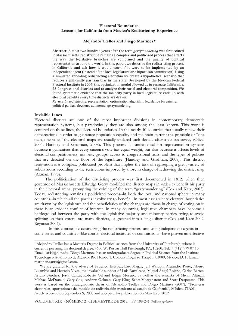
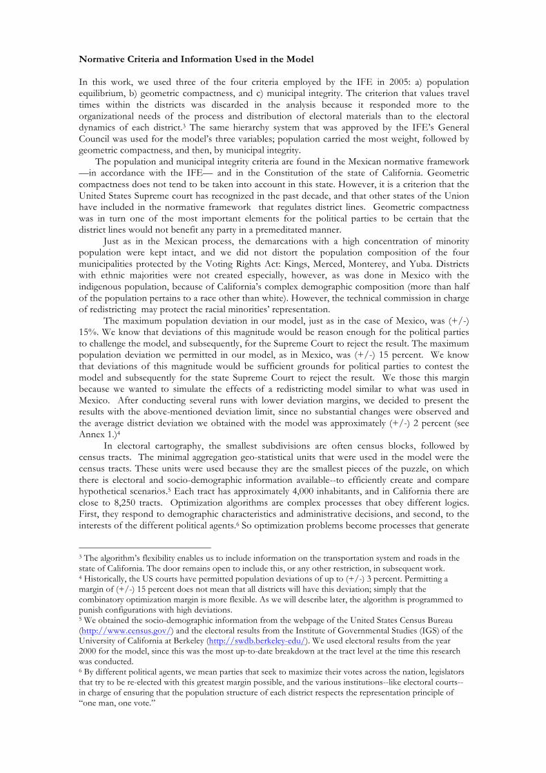
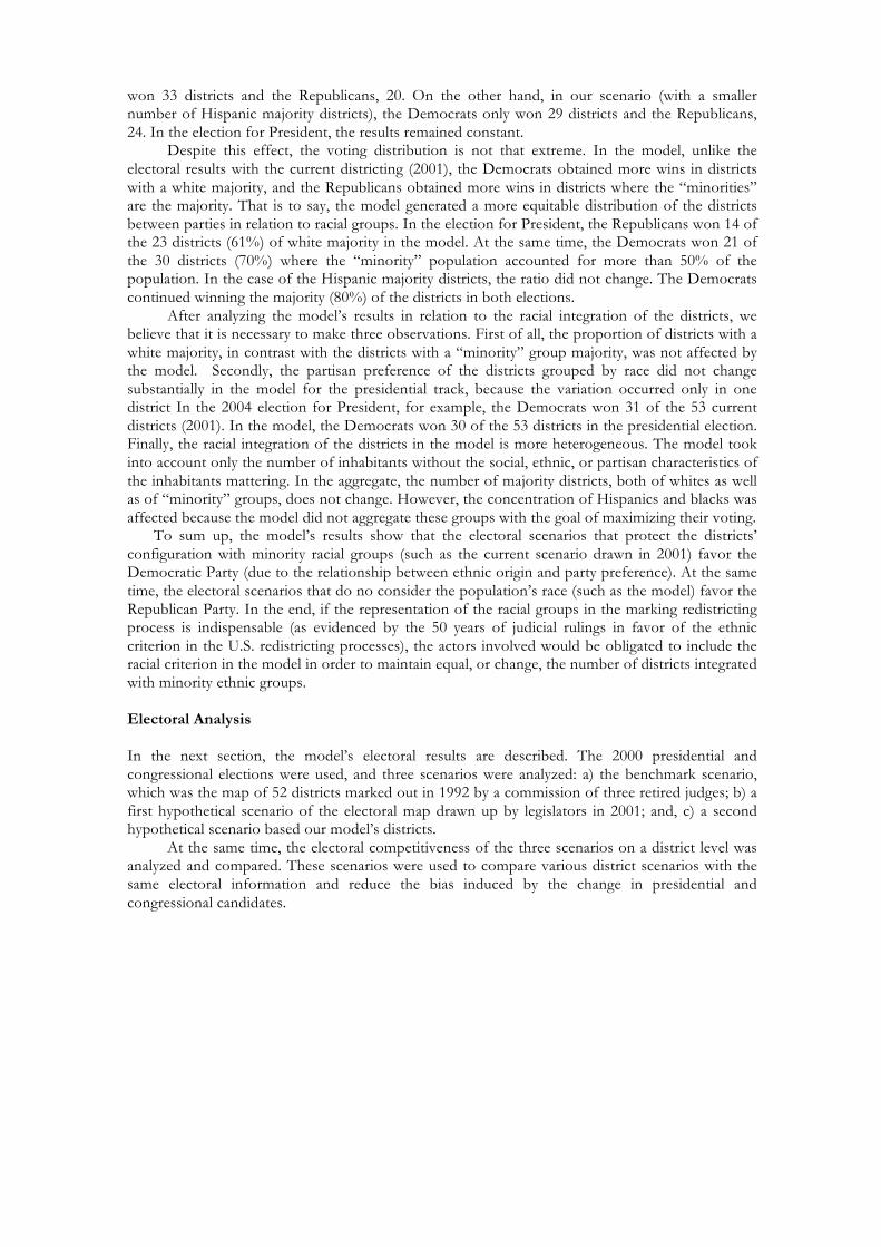
a result that maximizes the imposed restrictions, but always at the associated cost of punishing some variables in exchange for rewarding others (Papadimitriou and Steiglitz, 1998). Analysis of the system The simulated annealing method is a combinatory optimization algorithm that models the physical process of tempering metals. It was developed by Marshal Rosenbluth and Nicholas Metropolis in the 1950s (Metropolis et al., 1953). In the 1980s, some researchers interested in geo-spatial analysis began using this type of algorithm to solve optimization problems (Kirkpatrick et al., 1983). The model seeks to increase the cost (temperature) of the objective function and, after a cooling period, seeks the values that minimize the cost of the function. The process is repeated until an optimum result is obtained (Kirkpatrick et al., 1983; Gutiérrez et al., 1998; Macmillan, 2001; Antoniano, 2006; Joshi et al., 2009). The algorithm is defined based on four basic components: a) the configuration space; b) the transition model; c) the cost function; and d) the cooling scheme.7 The configuration space refers to the universe of valid solutions from which the model seeks an optimum result. In this case, we establish that a valid configuration is a division of a set U of geographic units into N subsets or districts, where every geographic unit belongs to a single district, and every district is geographically continuous. The transition model is the set of rules that enable us to generate one configuration based on another, so that neighboring groups of sets can be generated in a single step. The transitions allow us to introduce the random component in successive optimization, where a transition is the change in one district based on the change in a single geographic unit. In the model, a unit can only move to a contiguous district, and the district to which that unit belongs must remain continuous. The cost function is the framework for evaluating a configuration. It represents the weighted average of partial functions that respond to the criteria imposed by the agent in charge of drawing the electoral map. The model associates a value to each configuration and seeks and optimum result that minimizes the cost function. Finally, the cooling scheme is a series of rules that permit the model to adjust the “temperature” and find an optimum solution. This component includes factors such as initial temperature, temperature changes, number of iterations--or length of the internal cycle--and the criteria for stopping the algorithm when an optimum solution is found (Antoniano, 2006). The model begins the search for an optimum solution by raising the initial temperature--which depends on the variations generated by the cost function. For the model, it doesn’t matter if results worsen at the start, since the algorithm permits all changes in state found within the configuration space. As the temperature drops, the restrictions of the algorithm do not permit movements that surpass the value associated with the last maximum cost of the function, and only admit changes within the temperature limit. As the cost drops during the cooling, the result of the function approaches zero. When the system no longer finds favorable changes, it stops and reaches a freeze point (see figure 1). The cost function is the “heart” of the model (see Annex 2). It is responsible for evaluating the movements made within the system and for validating or penalizing each one of them through three central components. The population variable had the greatest weight in the model, and we assigned it a weight of a1 = .5; followed by geographic compactness, with a weight of a1 = .3; and finally, municipal integrity, with a weighting of a2 = .2. Like the model used by the IFE in 2005, the cost function found a minimum when the population deviation of most districts approached the population average for the state (state population/53 districts), when the districts took on a compact geometric form and when municipalities that had enough inhabitants to form a district were not fragmented.

7 For a detailed analysis of the use of the simulated annealing method in redistricting processes, see Antoniano (2006), “El recocido simulado aplicado al problema de redistritacio ́n electoral”.

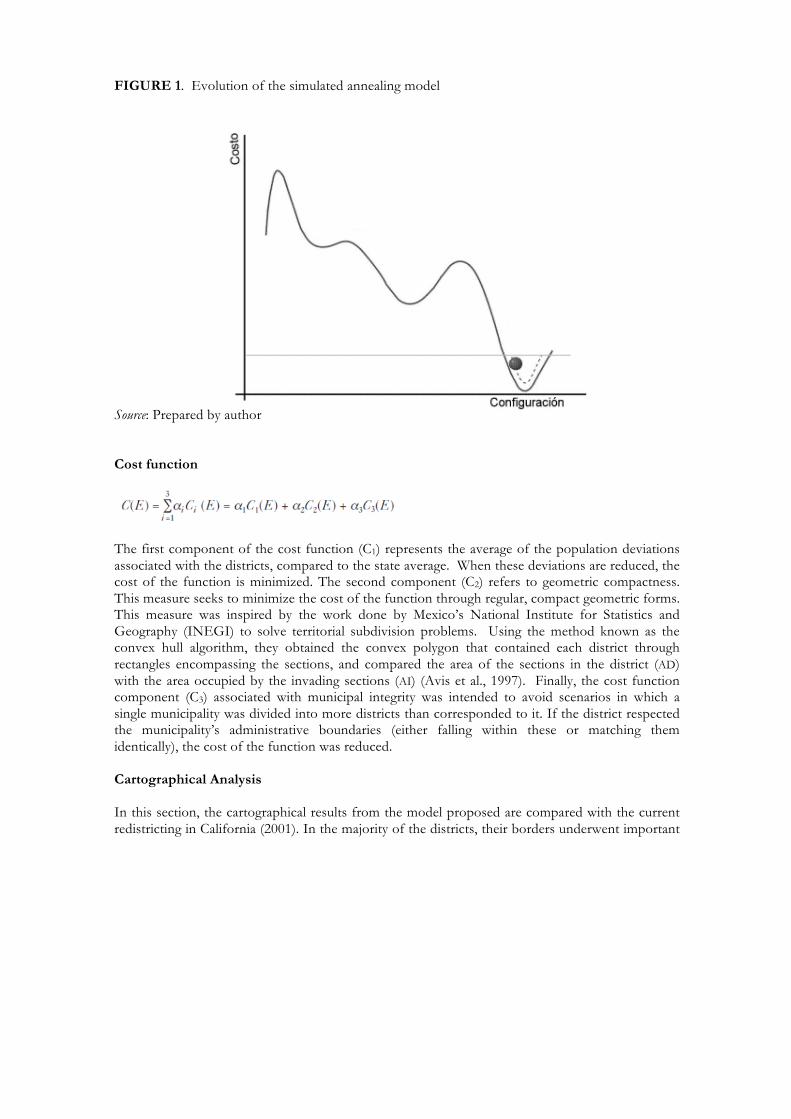
FIGURE 1. Evolution of the simulated annealing model Source: Prepared by author Cost function

The first component of the cost function (C1) represents the average of the population deviations associated with the districts, compared to the state average. When these deviations are reduced, the cost of the function is minimized. The second component (C2) refers to geometric compactness. This measure seeks to minimize the cost of the function through regular, compact geometric forms. This measure was inspired by the work done by Mexico’s National Institute for Statistics and Geography (INEGI) to solve territorial subdivision problems. Using the method known as the convex hull algorithm, they obtained the convex polygon that contained each district through rectangles encompassing the sections, and compared the area of the sections in the district (AD) with the area occupied by the invading sections (AI) (Avis et al., 1997). Finally, the cost function component (C3) associated with municipal integrity was intended to avoid scenarios in which a single municipality was divided into more districts than corresponded to it. If the district respected the municipality’s administrative boundaries (either falling within these or matching them identically), the cost of the function was reduced. Cartographical Analysis In this section, the cartographical results from the model proposed are compared with the current redistricting in California (2001). In the majority of the districts, their borders underwent important

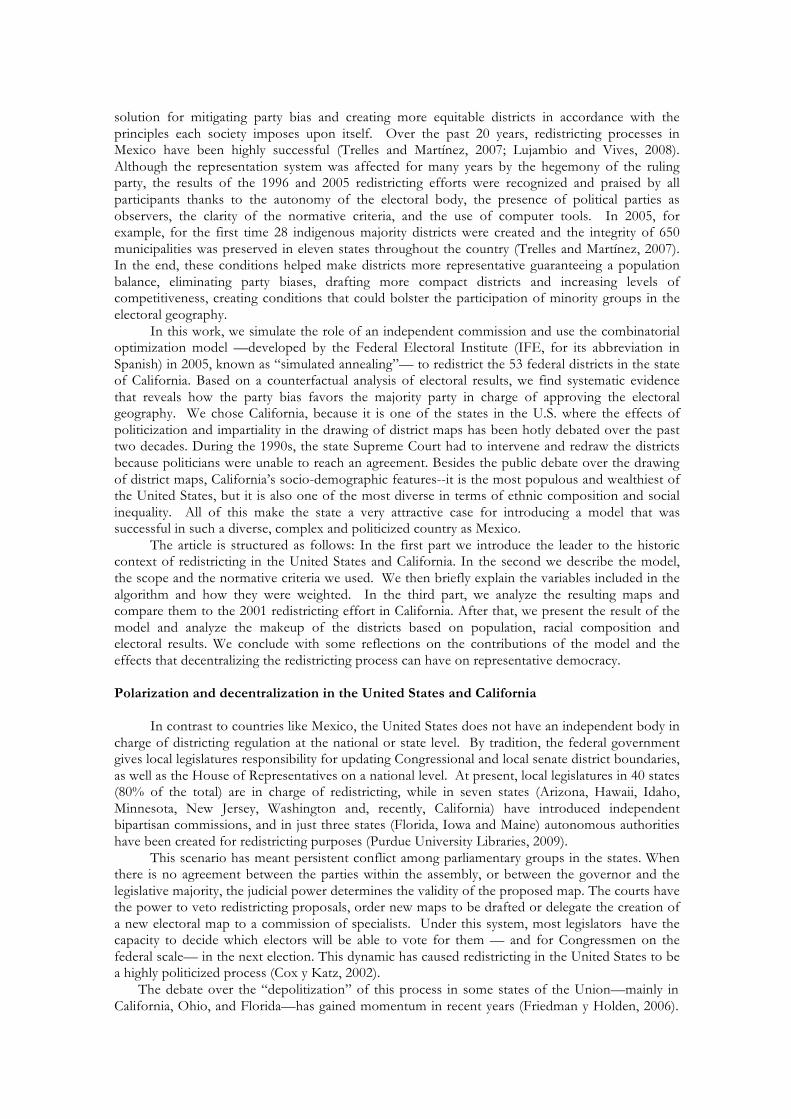
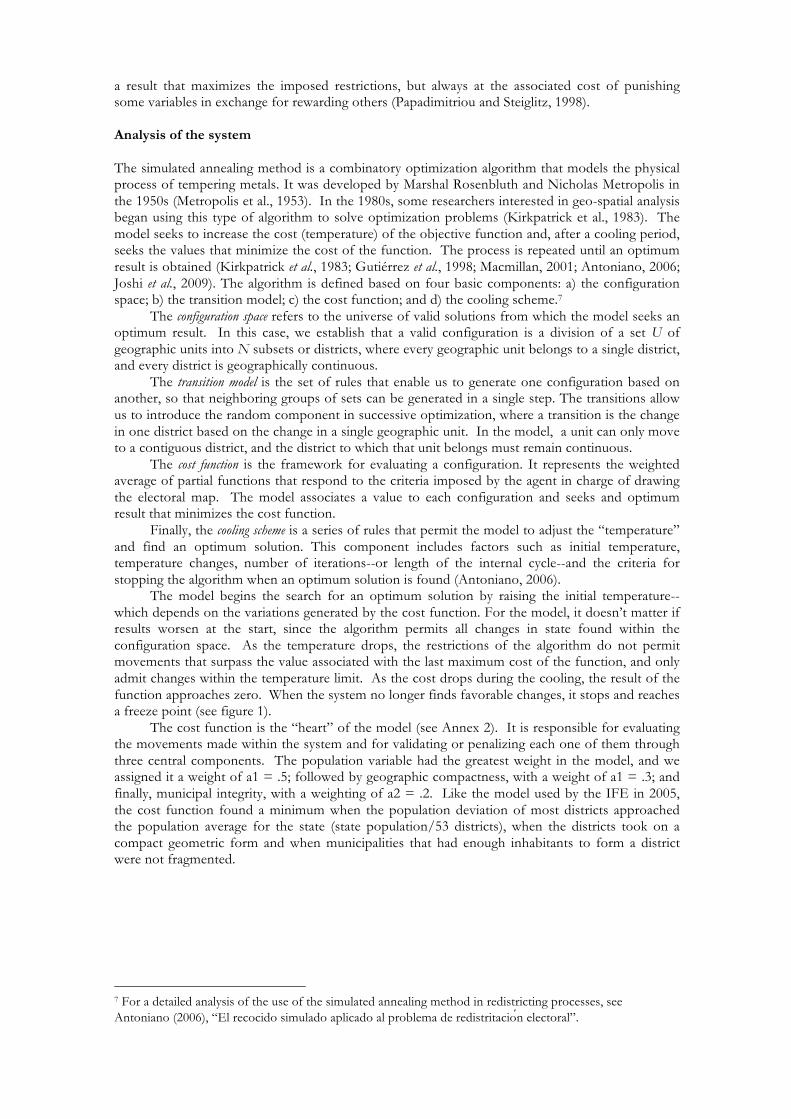
Map 1. Los Angeles Area close-up - 2001

Source: Prepared by author changes. In general, the model produced more compact districts and eliminated the irregular shapes that prevail in the urban areas of the current districting. District compactness is one of the criteria that the Supreme Court has traditionally maintained in order to detect if there is partisan gerrymandering (Altman, 1998). We made a close-up of the areas that visually evidence some partisan interest in the redistricting process and we compared them with the model’s results.

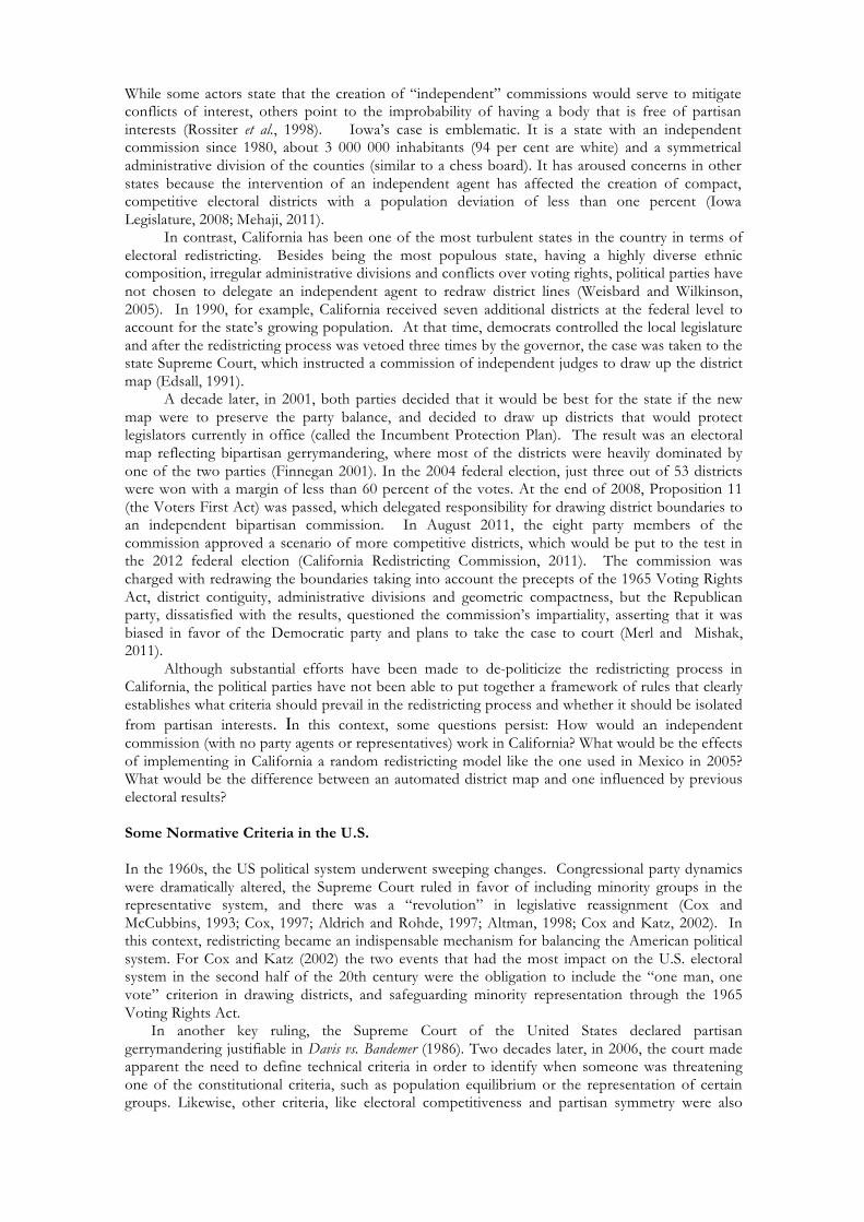
Importance was given to the geometric compactness criterion for two reasons. Firstly, because we sought to simulate the redistricting conditions that took place in Mexico in 2005; and secondly, because compactness, as part of a random combinatorial optimization model, substantially diminishes the probability of finding partisan lines that arbitrarily group together or divide electoral bastions. As we can observe in Map 1,8 which shows the Los Angeles area, there are five current districts that are fragmented into three counties adjacent to Los Angeles: Ventura, Orange, and San Bernardino. On the other hand, in Map 2 of the Los Angeles area, there are only two districts that share territory with Ventura County (to the north of Los Angeles). The rest are located within Los Angeles County in their totality. This is due to the assignment that we did within the municipalities.

Map 2. Los Angeles Area close-up - model

Source: Prepared by author

8 The figures in this publication can be viewed in color on the webpage of one of the authors (www.alejandrotrelles.com) or on the Política y Gobierno website.

Maps 1 and 2 show that the district borders from the model delimit units significantly more regular in shape than those of the current outline. In addition, the results of the model follow more closely the criteria of municipal integrity, considered in the California Constitution, because it has only one municipality split into two districts instead of three municipalities split into five.

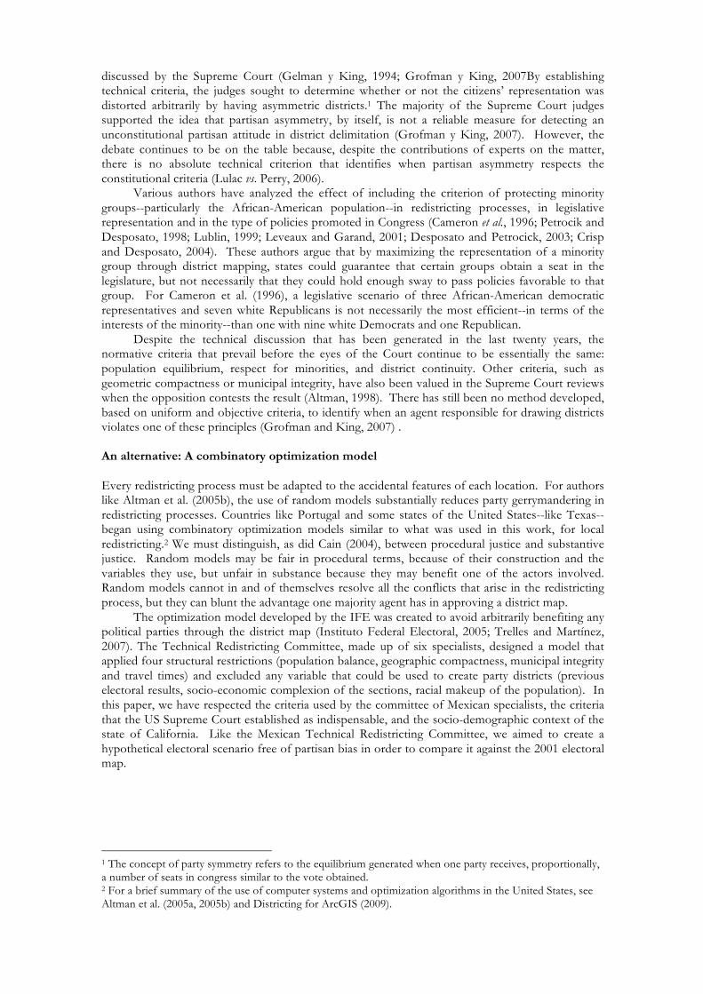
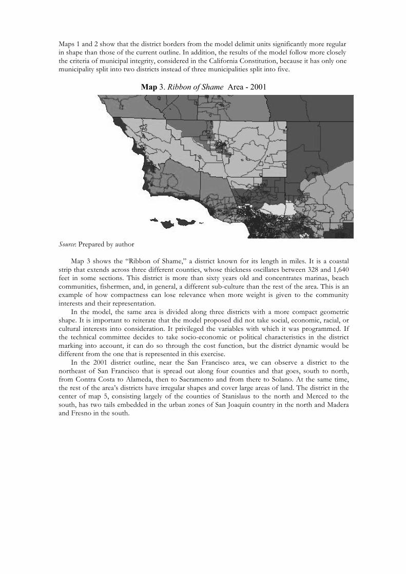
Map 3. Ribbon of Shame Area - 2001

Source: Prepared by author

Map 3 shows the “Ribbon of Shame,” a district known for its length in miles. It is a coastal

strip that extends across three different counties, whose thickness oscillates between 328 and 1,640 feet in some sections. This district is more than sixty years old and concentrates marinas, beach communities, fishermen, and, in general, a different sub-culture than the rest of the area. This is an example of how compactness can lose relevance when more weight is given to the community interests and their representation.

In the model, the same area is divided along three districts with a more compact geometric shape. It is important to reiterate that the model proposed did not take social, economic, racial, or cultural interests into consideration. It privileged the variables with which it was programmed. If the technical committee decides to take socio-economic or political characteristics in the district marking into account, it can do so through the cost function, but the district dynamic would be different from the one that is represented in this exercise.

In the 2001 district outline, near the San Francisco area, we can observe a district to the northeast of San Francisco that is spread out along four counties and that goes, south to north, from Contra Costa to Alameda, then to Sacramento and from there to Solano. At the same time, the rest of the area’s districts have irregular shapes and cover large areas of land. The district in the center of map 5, consisting largely of the counties of Stanislaus to the north and Merced to the south, has two tails embedded in the urban zones of San Joaquín country in the north and Madera and Fresno in the south.

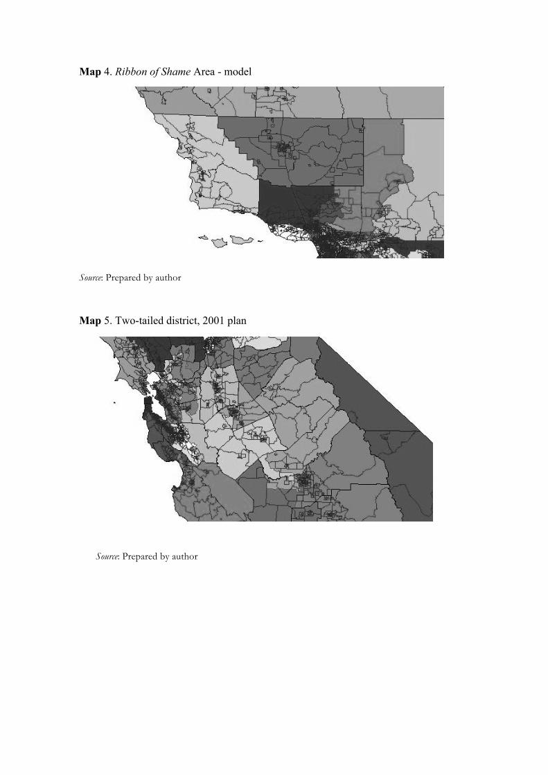
Map 4. Ribbon of Shame Area - model

Source: Prepared by author

Map 5. Two-tailed district, 2001 plan

Source: Prepared by author

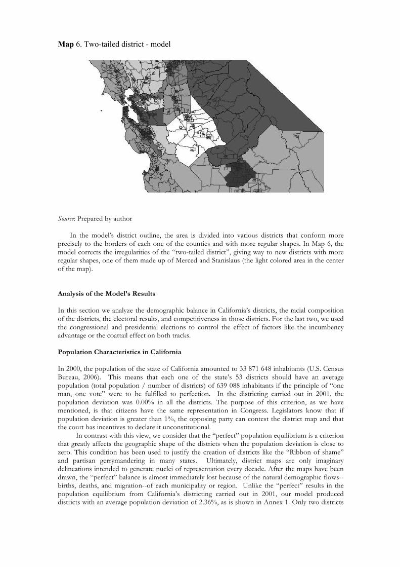
Map 6. Two-tailed district - model

Source: Prepared by author

In the model’s district outline, the area is divided into various districts that conform more

precisely to the borders of each one of the counties and with more regular shapes. In Map 6, the model corrects the irregularities of the “two-tailed district”, giving way to new districts with more regular shapes, one of them made up of Merced and Stanislaus (the light colored area in the center of the map).

Analysis of the Model’s Results In this section we analyze the demographic balance in California’s districts, the racial composition of the districts, the electoral results, and competitiveness in those districts. For the last two, we used the congressional and presidential elections to control the effect of factors like the incumbency advantage or the coattail effect on both tracks. Population Characteristics in California In 2000, the population of the state of California amounted to 33 871 648 inhabitants (U.S. Census Bureau, 2006). This means that each one of the state’s 53 districts should have an average population (total population / number of districts) of 639 088 inhabitants if the principle of “one man, one vote” were to be fulfilled to perfection. In the districting carried out in 2001, the population deviation was 0.00% in all the districts. The purpose of this criterion, as we have mentioned, is that citizens have the same representation in Congress. Legislators know that if population deviation is greater than 1%, the opposing party can contest the district map and that the court has incentives to declare it unconstitutional. In contrast with this view, we consider that the “perfect” population equilibrium is a criterion that greatly affects the geographic shape of the districts when the population deviation is close to zero. This condition has been used to justify the creation of districts like the “Ribbon of shame” and partisan gerrymandering in many states. Ultimately, district maps are only imaginary delineations intended to generate nuclei of representation every decade. After the maps have been drawn, the “perfect” balance is almost immediately lost because of the natural demographic flows--births, deaths, and migration--of each municipality or region. Unlike the “perfect” results in the population equilibrium from California’s districting carried out in 2001, our model produced districts with an average population deviation of 2.36%, as is shown in Annex 1. Only two districts

had population deviations greater than 10%: one was 10.45%, and the other, larger one, was -11.81%. The smallest population deviation was 0.01 percent (Annex 1)

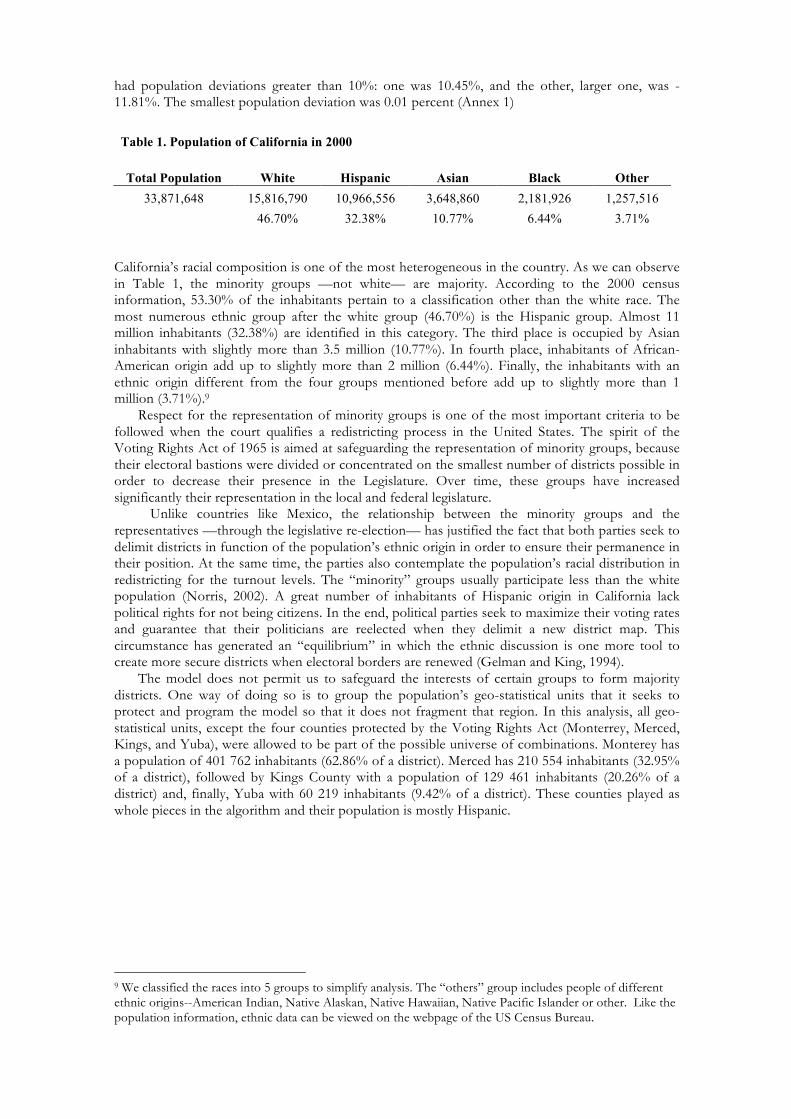
Table 1. Population of California in 2000

Total Population White Hispanic Asian Black Other 33,871,648 15,816,790 10,966,556 3,648,860 2,181,926 1,257,516

46.70% 32.38% 10.77% 6.44% 3.71%

California’s racial composition is one of the most heterogeneous in the country. As we can observe in Table 1, the minority groups —not white— are majority. According to the 2000 census information, 53.30% of the inhabitants pertain to a classification other than the white race. The most numerous ethnic group after the white group (46.70%) is the Hispanic group. Almost 11 million inhabitants (32.38%) are identified in this category. The third place is occupied by Asian inhabitants with slightly more than 3.5 million (10.77%). In fourth place, inhabitants of African-American origin add up to slightly more than 2 million (6.44%). Finally, the inhabitants with an ethnic origin different from the four groups mentioned before add up to slightly more than 1 million (3.71%).9

Respect for the representation of minority groups is one of the most important criteria to be followed when the court qualifies a redistricting process in the United States. The spirit of the Voting Rights Act of 1965 is aimed at safeguarding the representation of minority groups, because their electoral bastions were divided or concentrated on the smallest number of districts possible in order to decrease their presence in the Legislature. Over time, these groups have increased significantly their representation in the local and federal legislature.

Unlike countries like Mexico, the relationship between the minority groups and the representatives ––through the legislative re-election–– has justified the fact that both parties seek to delimit districts in function of the population’s ethnic origin in order to ensure their permanence in their position. At the same time, the parties also contemplate the population’s racial distribution in redistricting for the turnout levels. The “minority” groups usually participate less than the white population (Norris, 2002). A great number of inhabitants of Hispanic origin in California lack political rights for not being citizens. In the end, political parties seek to maximize their voting rates and guarantee that their politicians are reelected when they delimit a new district map. This circumstance has generated an “equilibrium” in which the ethnic discussion is one more tool to create more secure districts when electoral borders are renewed (Gelman and King, 1994).

The model does not permit us to safeguard the interests of certain groups to form majority districts. One way of doing so is to group the population’s geo-statistical units that it seeks to protect and program the model so that it does not fragment that region. In this analysis, all geo-statistical units, except the four counties protected by the Voting Rights Act (Monterrey, Merced, Kings, and Yuba), were allowed to be part of the possible universe of combinations. Monterey has a population of 401 762 inhabitants (62.86% of a district). Merced has 210 554 inhabitants (32.95% of a district), followed by Kings County with a population of 129 461 inhabitants (20.26% of a district) and, finally, Yuba with 60 219 inhabitants (9.42% of a district). These counties played as whole pieces in the algorithm and their population is mostly Hispanic.

9 We classified the races into 5 groups to simplify analysis. The “others” group includes people of different ethnic origins--American Indian, Native Alaskan, Native Hawaiian, Native Pacific Islander or other. Like the population information, ethnic data can be viewed on the webpage of the US Census Bureau.

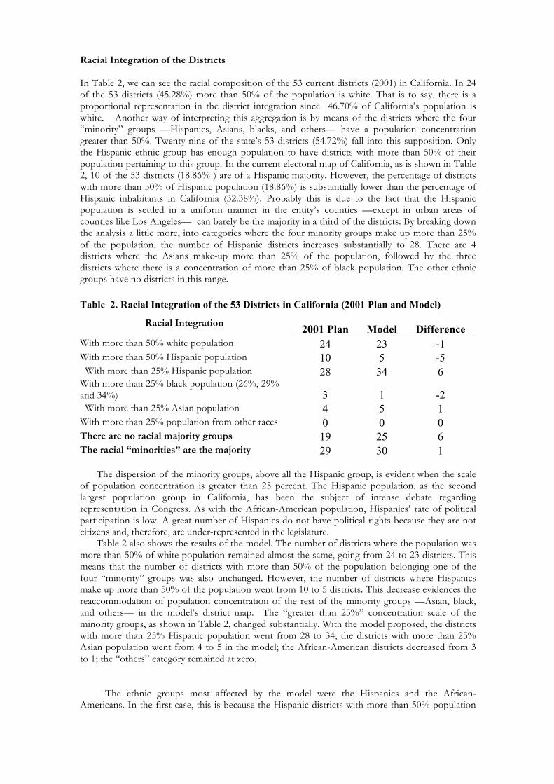
Racial Integration of the Districts In Table 2, we can see the racial composition of the 53 current districts (2001) in California. In 24 of the 53 districts (45.28%) more than 50% of the population is white. That is to say, there is a proportional representation in the district integration since 46.70% of California’s population is white. Another way of interpreting this aggregation is by means of the districts where the four “minority” groups —Hispanics, Asians, blacks, and others— have a population concentration greater than 50%. Twenty-nine of the state’s 53 districts (54.72%) fall into this supposition. Only the Hispanic ethnic group has enough population to have districts with more than 50% of their population pertaining to this group. In the current electoral map of California, as is shown in Table 2, 10 of the 53 districts (18.86% ) are of a Hispanic majority. However, the percentage of districts with more than 50% of Hispanic population (18.86%) is substantially lower than the percentage of Hispanic inhabitants in California (32.38%). Probably this is due to the fact that the Hispanic population is settled in a uniform manner in the entity’s counties —except in urban areas of counties like Los Angeles— can barely be the majority in a third of the districts. By breaking down the analysis a little more, into categories where the four minority groups make up more than 25% of the population, the number of Hispanic districts increases substantially to 28. There are 4 districts where the Asians make-up more than 25% of the population, followed by the three districts where there is a concentration of more than 25% of black population. The other ethnic groups have no districts in this range. Table 2. Racial Integration of the 53 Districts in California (2001 Plan and Model)

Racial Integration 2001 Plan Model Difference With more than 50% white population 24 23 -1 With more than 50% Hispanic population 10 5 -5 With more than 25% Hispanic population 28 34 6 With more than 25% black population (26%, 29% and 34%) 3 1 -2 With more than 25% Asian population 4 5 1 With more than 25% population from other races 0 0 0 There are no racial majority groups 19 25 6 The racial “minorities” are the majority 29 30 1

The dispersion of the minority groups, above all the Hispanic group, is evident when the scale of population concentration is greater than 25 percent. The Hispanic population, as the second largest population group in California, has been the subject of intense debate regarding representation in Congress. As with the African-American population, Hispanics’ rate of political participation is low. A great number of Hispanics do not have political rights because they are not citizens and, therefore, are under-represented in the legislature.

Table 2 also shows the results of the model. The number of districts where the population was more than 50% of white population remained almost the same, going from 24 to 23 districts. This means that the number of districts with more than 50% of the population belonging one of the four “minority” groups was also unchanged. However, the number of districts where Hispanics make up more than 50% of the population went from 10 to 5 districts. This decrease evidences the reaccommodation of population concentration of the rest of the minority groups —Asian, black, and others— in the model’s district map. The “greater than 25%” concentration scale of the minority groups, as shown in Table 2, changed substantially. With the model proposed, the districts with more than 25% Hispanic population went from 28 to 34; the districts with more than 25% Asian population went from 4 to 5 in the model; the African-American districts decreased from 3 to 1; the “others” category remained at zero.

The ethnic groups most affected by the model were the Hispanics and the African-Americans. In the first case, this is because the Hispanic districts with more than 50% population

concentration went from 10 to 5. However, the distribution of the Hispanic population in districts with more than 25% population also changed substantially. They went from 28 to 34 districts in the model. In the second case, the districts with more than 25% black population went from 3 to 1 in the model. However, upon reviewing the black population percentage in each district, we detected that in the 3 current districts with more than 25% black population the concentration was 26%, 29%, and 34%. On the other hand, the black population from the only district with more 25% population of this ethnic group in the model was 44 percent. The results show how the model, in a first scenario, leaves the lobbying interests of different groups aside —in this case the racial groups— in order to be represented in the congresses. The model interprets the numbers that it processes as quantity of people that inhabit a place; it does not identify them by race, social status, or partisan preference. However, if the technical committee wished to take these characteristics into account in the marking out of districts, they could be included in the model. In the case of the Hispanic group, it is probable that they have maximized their representation in the districts through political lobbying. In the case of the African-American population, it is likely that their representatives have lobbied to have a significant representation in three districts instead of being concentrated in one single district as shown in the model. The Asian ethnic group obtained an additional district on the greater than 25% population concentration scale. This is probably due to the fact that the model reflected the size of the third most numerous group in California after the whites and the Hispanics. In the aggregate, the majority white district composition and the districts comprising the four minority groups did not change drastically. We understand that the decrease in the number of majority Hispanic districts would be an obstacle and that the parties (especially the Democratic party) would contest the proposed model’s scenario before the court. If an autonomous commission were in charge of redrawing districts, it would probably be forced to take racial minority groups into account. In that scenario, the commission would have to define the minimum number of districts according to each ethnic group and the mechanisms to seek the representation of all the racial groups in Congress. As has happened in some other places that have used optimization models, the lobbying could be done once the model has produced a first scenario.

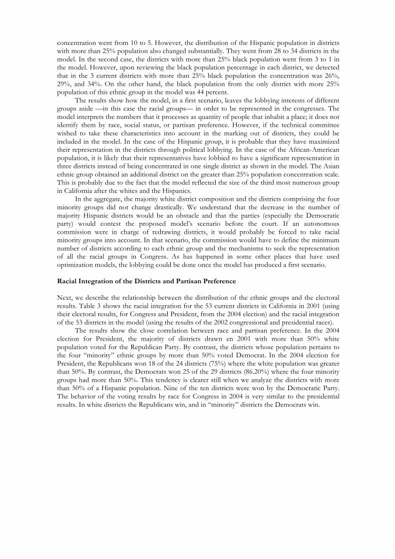
Racial Integration of the Districts and Partisan Preference Next, we describe the relationship between the distribution of the ethnic groups and the electoral results. Table 3 shows the racial integration for the 53 current districts in California in 2001 (using their electoral results, for Congress and President, from the 2004 election) and the racial integration of the 53 districts in the model (using the results of the 2002 congressional and presidential races). The results show the close correlation between race and partisan preference. In the 2004 election for President, the majority of districts drawn en 2001 with more than 50% white population voted for the Republican Party. By contrast, the districts whose population pertains to the four “minority” ethnic groups by more than 50% voted Democrat. In the 2004 election for President, the Republicans won 18 of the 24 districts (75%) where the white population was greater than 50%. By contrast, the Democrats won 25 of the 29 districts (86.20%) where the four minority groups had more than 50%. This tendency is clearer still when we analyze the districts with more than 50% of a Hispanic population. Nine of the ten districts were won by the Democratic Party. The behavior of the voting results by race for Congress in 2004 is very similar to the presidential results. In white districts the Republicans win, and in “minority” districts the Democrats win.

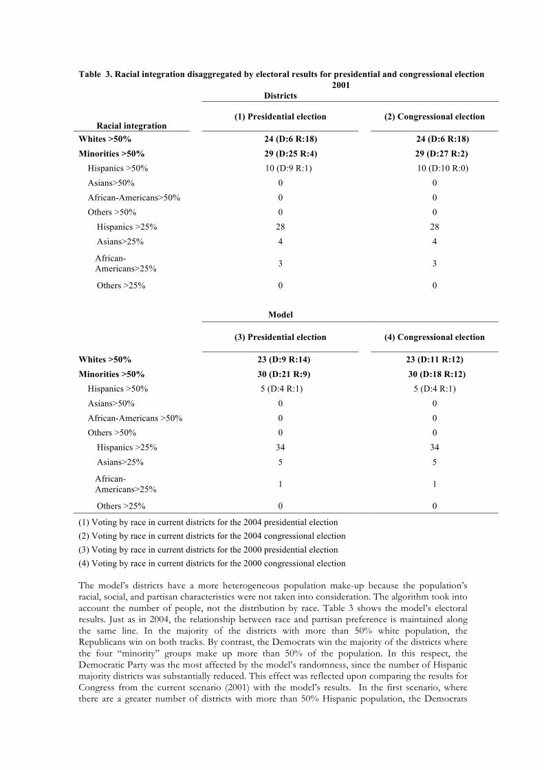
Table 3. Racial integration disaggregated by electoral results for presidential and congressional election

2001 Districts

Racial integration

(1) Presidential election (2) Congressional election

Whites >50% 24 (D:6 R:18) 24 (D:6 R:18) Minorities >50% 29 (D:25 R:4) 29 (D:27 R:2) Hispanics >50% 10 (D:9 R:1) 10 (D:10 R:0) Asians>50% 0 0 African-Americans>50% 0 0 Others >50% 0 0 Hispanics >25% 28 28 Asians>25% 4 4

African- Americans>25% 3 3

Others >25% 0 0

Model

(3) Presidential election (4) Congressional election

Whites >50%

23 (D:9 R:14) 23 (D:11 R:12) Minorities >50%

30 (D:21 R:9) 30 (D:18 R:12)

Hispanics >50%

5 (D:4 R:1) 5 (D:4 R:1) Asians>50%

0 0

African-Americans >50%

0 0 Others >50%

0 0

Hispanics >25%

34 34 Asians>25%

5 5

African- Americans>25%

1 1

Others >25% 0 0

(1) Voting by race in current districts for the 2004 presidential election (2) Voting by race in current districts for the 2004 congressional election (3) Voting by race in current districts for the 2000 presidential election (4) Voting by race in current districts for the 2000 congressional election The model’s districts have a more heterogeneous population make-up because the population’s racial, social, and partisan characteristics were not taken into consideration. The algorithm took into account the number of people, not the distribution by race. Table 3 shows the model’s electoral results. Just as in 2004, the relationship between race and partisan preference is maintained along the same line. In the majority of the districts with more than 50% white population, the Republicans win on both tracks. By contrast, the Democrats win the majority of the districts where the four “minority” groups make up more than 50% of the population. In this respect, the Democratic Party was the most affected by the model’s randomness, since the number of Hispanic majority districts was substantially reduced. This effect was reflected upon comparing the results for Congress from the current scenario (2001) with the model’s results. In the first scenario, where there are a greater number of districts with more than 50% Hispanic population, the Democrats

won 33 districts and the Republicans, 20. On the other hand, in our scenario (with a smaller number of Hispanic majority districts), the Democrats only won 29 districts and the Republicans, 24. In the election for President, the results remained constant. Despite this effect, the voting distribution is not that extreme. In the model, unlike the electoral results with the current districting (2001), the Democrats obtained more wins in districts with a white majority, and the Republicans obtained more wins in districts where the “minorities” are the majority. That is to say, the model generated a more equitable distribution of the districts between parties in relation to racial groups. In the election for President, the Republicans won 14 of the 23 districts (61%) of white majority in the model. At the same time, the Democrats won 21 of the 30 districts (70%) where the “minority” population accounted for more than 50% of the population. In the case of the Hispanic majority districts, the ratio did not change. The Democrats continued winning the majority (80%) of the districts in both elections. After analyzing the model’s results in relation to the racial integration of the districts, we believe that it is necessary to make three observations. First of all, the proportion of districts with a white majority, in contrast with the districts with a “minority” group majority, was not affected by the model. Secondly, the partisan preference of the districts grouped by race did not change substantially in the model for the presidential track, because the variation occurred only in one district In the 2004 election for President, for example, the Democrats won 31 of the 53 current districts (2001). In the model, the Democrats won 30 of the 53 districts in the presidential election. Finally, the racial integration of the districts in the model is more heterogeneous. The model took into account only the number of inhabitants without the social, ethnic, or partisan characteristics of the inhabitants mattering. In the aggregate, the number of majority districts, both of whites as well as of “minority” groups, does not change. However, the concentration of Hispanics and blacks was affected because the model did not aggregate these groups with the goal of maximizing their voting.

To sum up, the model’s results show that the electoral scenarios that protect the districts’ configuration with minority racial groups (such as the current scenario drawn in 2001) favor the Democratic Party (due to the relationship between ethnic origin and party preference). At the same time, the electoral scenarios that do no consider the population’s race (such as the model) favor the Republican Party. In the end, if the representation of the racial groups in the marking redistricting process is indispensable (as evidenced by the 50 years of judicial rulings in favor of the ethnic criterion in the U.S. redistricting processes), the actors involved would be obligated to include the racial criterion in the model in order to maintain equal, or change, the number of districts integrated with minority ethnic groups.

Electoral Analysis In the next section, the model’s electoral results are described. The 2000 presidential and congressional elections were used, and three scenarios were analyzed: a) the benchmark scenario, which was the map of 52 districts marked out in 1992 by a commission of three retired judges; b) a first hypothetical scenario of the electoral map drawn up by legislators in 2001; and, c) a second hypothetical scenario based our model’s districts. At the same time, the electoral competitiveness of the three scenarios on a district level was analyzed and compared. These scenarios were used to compare various district scenarios with the same electoral information and reduce the bias induced by the change in presidential and congressional candidates.

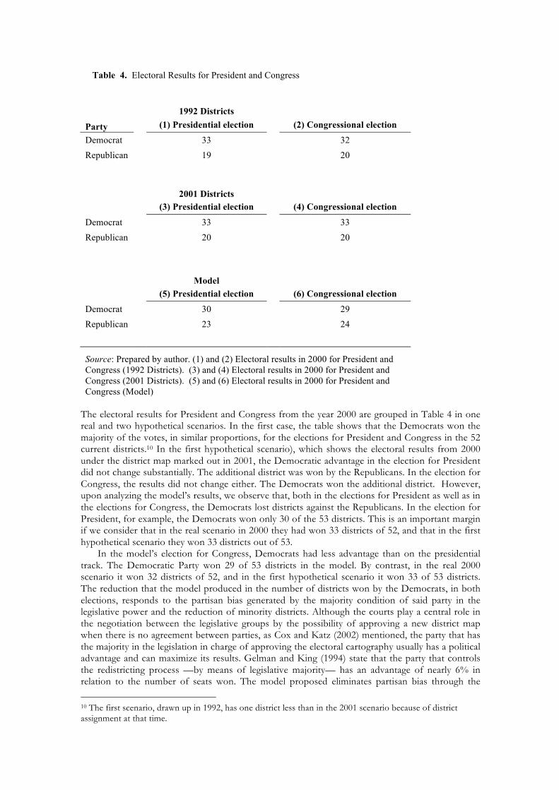
Table 4. Electoral Results for President and Congress

1992 Districts

Party

(1) Presidential election (2) Congressional election

Democrat 33 32 Republican 19 20

2001 Districts

(3) Presidential election (4) Congressional election

Democrat 33 33 Republican 20 20

Model

(5) Presidential election (6) Congressional election

Democrat 30 29 Republican 23 24

Source: Prepared by author. (1) and (2) Electoral results in 2000 for President and Congress (1992 Districts). (3) and (4) Electoral results in 2000 for President and Congress (2001 Districts). (5) and (6) Electoral results in 2000 for President and Congress (Model)

The electoral results for President and Congress from the year 2000 are grouped in Table 4 in one real and two hypothetical scenarios. In the first case, the table shows that the Democrats won the majority of the votes, in similar proportions, for the elections for President and Congress in the 52 current districts.10 In the first hypothetical scenario), which shows the electoral results from 2000 under the district map marked out in 2001, the Democratic advantage in the election for President did not change substantially. The additional district was won by the Republicans. In the election for Congress, the results did not change either. The Democrats won the additional district. However, upon analyzing the model’s results, we observe that, both in the elections for President as well as in the elections for Congress, the Democrats lost districts against the Republicans. In the election for President, for example, the Democrats won only 30 of the 53 districts. This is an important margin if we consider that in the real scenario in 2000 they had won 33 districts of 52, and that in the first hypothetical scenario they won 33 districts out of 53.

In the model’s election for Congress, Democrats had less advantage than on the presidential track. The Democratic Party won 29 of 53 districts in the model. By contrast, in the real 2000 scenario it won 32 districts of 52, and in the first hypothetical scenario it won 33 of 53 districts. The reduction that the model produced in the number of districts won by the Democrats, in both elections, responds to the partisan bias generated by the majority condition of said party in the legislative power and the reduction of minority districts. Although the courts play a central role in the negotiation between the legislative groups by the possibility of approving a new district map when there is no agreement between parties, as Cox and Katz (2002) mentioned, the party that has the majority in the legislation in charge of approving the electoral cartography usually has a political advantage and can maximize its results. Gelman and King (1994) state that the party that controls the redistricting process —by means of legislative majority— has an advantage of nearly 6% in relation to the number of seats won. The model proposed eliminates partisan bias through the

10 The first scenario, drawn up in 1992, has one district less than in the 2001 scenario because of district assignment at that time.

randomness of the algorithm and by not taking into account previous electoral results or the population’s socio-economic characteristics. The model’s results benefits the Republican Party in the state of California because they eliminate the advantage of the agent with the legislative capacity for approving the electoral cartography (Trelles, 2010). The first hypothetical scenario apparently contradicts Gelman and King’s theory (1994). However, in the next section on district competitiveness, we will see how the Democrats —who controlled the state legislature— benefited by increasing their victories in secure districts on both tracks.

Competitiveness in the Districts In this section, we analyze the competitiveness of the results for the elections for Congress and President in the benchmark scenario, in the first hypothetical scenario and in the scenario that the model generated. Competitiveness was classified in four categories in order to obtain more exact data. The “very competitive” districts are those where the difference between first and second place is less than 5%; the “competitive” districts are those where the difference is greater than or equal to 5% and less than 10%; the “secure” districts are those whose difference is greater than or equal to 10% and less than 15%; and, finally, the “very secure” districts are those where the difference between first and second place is more than or equal to 15 percent.

The results can be interpreted with different levels of rigidity. In this analysis of competitiveness, the districts were classified in terms of “competitive” districts —when the difference is less than 10%— and “secure” districts—when the difference is greater than or equal to 10 percent. In the redistricting processes the parties seek to maximize the number of districts won, and the politicians in office —incumbents— seek reelection. On occasion, these two interests oppose each other. The partisan agent or group in charge of delimiting the districts usually seeks to balance its decision in order to maximize the voting rate in the districts and not leave the incumbents exposed (Gelman and King, 1994).

Table 5 shows that in the 2000 election for President, in the benchmark scenario, there were 15 competitive districts and 37 secure districts. Of the 15 competitive districts, the Democratic Party won in 6 and the Republican Party won in the 9 remaining districts. By contrast, in the 37 secure districts, the Democrats won 27 districts and the Republicans only won ten. In the election for Congress from the same year, there were only 7 competitive districts and 45 secure districts. In other words, in the majority of the districts, the election was won with an advantage greater than ten percentage points. The Democratic Party won 26 of the secure districts and the Republicans won 19 districts. Of the 7 competitive districts, 6 went to the Democrats, and only one to the Republicans.

In Table 5, we can see that the number of competitive districts decreased significantly in the first hypothetical scenario. Unlike the previous (benchmark) scenario, in the election for President the competitive districts go from 15 to 6. Two of those are won by the Democrats, and four, by the Republicans. The rest of the 47 secure districts, in their majority, are won by the Democratic Party. It got 31 districts, while the Republican Party only won 16. In the election for Congress the districts are still less competitive than in the Presidential election. There is only one competitive district and the Democratic Party wins it. At the same time, the rest of the secure districts are won, in their majority, by the Democrats who got 32 victories against 20 for the Republicans.

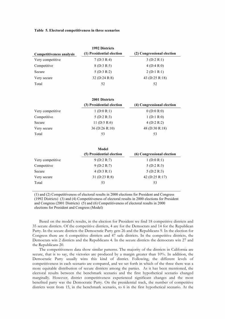
Table 5. Electoral competitiveness in three scenarios

1992 Districts

Competitiveness analysis

(1) Presidential election (2) Congressional election

Very competitive 7 (D:3 R:4) 3 (D:2 R:1) Competitive 8 (D:3 R:5) 4 (D:4 R:0) Secure 5 (D:3 R:2) 2 (D:1 R:1) Very secure 32 (D:24 R:8) 43 (D:25 R:18) Total 52 52

2001 Districts

(3) Presidential election (4) Congressional election

Very competitive 1 (D:0 R:1) 0 (D:0 R:0) Competitive 5 (D:2 R:3) 1 (D:1 R:0) Secure 11 (D:5 R:6) 4 (D:2 R:2) Very secure 36 (D:26 R:10) 48 (D:30 R:18) Total 53 53

Model

(5) Presidential election (6) Congressional election Very competitive 9 (D:2 R:7) 1 (D:0 R:1) Competitive 9 (D:2 R:7) 5 (D:2 R:3) Secure 4 (D:3 R:1) 5 (D:2 R:3) Very secure 31 (D:23 R:8) 42 (D:25 R:17) Total 53 53 (1) and (2) Competitiveness of electoral results in 2000 elections for President and Congress (1992 Districts) (3) and (4) Competitiveness of electoral results in 2000 elections for President and Congress (2001 Districts) (5) and (6) Competitiveness of electoral results in 2000 elections for President and Congress (Model)

Based on the model’s results, in the election for President we find 18 competitive districts and 35 secure districts. Of the competitive districts, 4 are for the Democrats and 14 for the Republican Party. In the secure districts the Democratic Party gets 26 and the Republicans 9. In the election for Congress there are 6 competitive districts and 47 safe districts. In the competitive districts, the Democrats win 2 districts and the Republicans 4. In the secure districts the democrats win 27 and the Republicans 20.

The competitiveness data show similar patterns. The majority of the districts in California are secure, that is to say, the victories are produced by a margin greater than 10%. In addition, the Democratic Party usually wins this kind of district. Following, the different levels of competitiveness in each scenario are compared, and we set forth in which of the three there was a more equitable distribution of secure districts among the parties. As it has been mentioned, the electoral results between the benchmark scenario and the first hypothetical scenario changed marginally. However, district competitiveness experienced significant changes and the most benefited party was the Democratic Party. On the presidential track, the number of competitive districts went from 15, in the benchmark scenario, to 6 in the first hypothetical scenario. At the

same time, the Democrats significantly increased their victories in the secure districts. They went from 27 in the benchmark scenario to 31 in the first hypothetical scenario. In the case of the Congress, the effect was similar: the competitive districts went from 7, in the benchmark scenario, to just 1 in the first hypothetical scenario. At the same time, the Democrats increased their victories significantly in the secure districts. They went from 26 districts, in the benchmark scenario, to 32 in the hypothetical scenario. These data reflect the Democratic Party’s interest in approving the district marking in 2001. The global marker did not suffer major changes, but the Democratic victories in the secure districts increased notably.

Upon comparing the benchmark scenario with the model’s results, we can observe that the Democratic Party’s advantage in the total number of districts won decreased substantially on both tracks. As far as competitiveness, we can observe two effects: a) the number of competitive districts increased on the presidential track and was maintained constant with the model in the legislative arena, and b) the Republican Party recovered an important number of competitive districts. In the election for President, the competitive districts went from 15, in the benchmark scenario, to 18 in the model’s scenario. The Republicans went from 9 victories in competitive districts to 14 in the model. The secure districts decreased and went from 37, in the real scenario, to 35. In this arena, the Republicans maintained their wins constant despite going from 10 to 9 districts. In the election for Congress the number of competitive districts hardly changed. They went from 7 districts, in the benchmark scenario, to 6 in the model. However, the number of Republican victories in this kind of district went from 1, in the real scenario, to 4 in the model’s scenario. The number of secure districts remained constant. It went from 45, in the real scenario, to 47 in the model’s scenario. At the same time, the Republican Party’s wins did not change substantially. They went from winning 19 secure districts in the real scenario, to 20 in the model’s scenario.

In summary, the proposed model produced the scenario with the greatest number of competitive districts (similar to the one marked out by the judges in 1992). In 2001, it is likely that the parties have come to an agreement on the number of secure districts that each one would get based on a similar simulation to the one from our first hypothetical scenario. The 2001 redistricting reduced competitiveness in the state and granted the Republican Party more secure districts, unlike those that it had in the previous district map, marked out in 1992, since they went from 10 secure districts, in the benchmark scenario, to 16 in the first hypothetical scenario, on the presidential track, and in the legislative election they went from 19 secure districts to 20 in the hypothetical scenario. Upon comparing the benchmark scenario with the one that the model produced, it is striking that the gap between first and second place has changed by approximately six percentage points. By considering only demographic information, and leaving aside the population’s ethnic, socio-economic, and electoral characteristics, the model eliminated the bias that could have generated the legislative advantage from the Democratic Party in order to mark out the districts as Gelman and King indicate (1994). Conclusions Every decade, most states in the U.S., and in many other countries of the world, are enmeshed in a political conflict over the redrawing of electoral districts. In this paper, we offer a possible way out of this type of conflict, through a decentralization of the redistricting process and the use of optimization models that mitigate partisan conflicts of interest. We show how the use of tools such as the simulated annealing model can be used to create more compact, unbiased districts, which minimize the restrictions imposed by the various political agents. We also offer evidence of a party bias that tends to favor the majority party in charge of approving the electoral map. When the rules of the game are not well defined, independent commissions are also tainted by party bias. More than a decade ago, Johnston et al. (1998) evidenced the case of the partisan impact of a “non-partisan” commission in Northern Ireland. If the political participants do not agree on rules so that the redistricting process is impartial, there is nothing that can be done. For this reason, it is important for the normative criteria to be exhaustive and endorsed by all of the agents involved in the redistricting effort. An independent group of specialists can be tremendously helpful in drawing up more equitable electoral maps when there is a precise regulatory framework endorsed by all the political parties. Along the same lines, technology can be used to improve the fairness of redistricting efforts or to benefit some political party. The success of these instruments depends on the working

relationship and interaction between interested arties, not in the operation of the algorithms. A quantitative assessment of the variables that can be included in the optimization model allows for specialists’ decisions, political party challenges to the scenario, or court rulings, to be formulated on the basis of technical criteria. The results of this research contribute evidence of the advantages of using optimization models in redistricting and schemes in which legislative chambers are not responsible for defining electoral boundaries. Additionally, we conclude that the virtues of decentralization and technology are not broad enough in and of themselves to depoliticize the redistricting process. Ultimately, it is crucial that the agents involved are convinced that, in a democracy, a central principle is that voters should elect their representatives, not that the representatives choose their voters. References

ALDRICH, John H. y David W. Rohde (1997), “The Transition to Republican Rule in the House: Implications for Theories of Congressional Politics”, Political Science Quarterly, 112, pp. 541­567. ALTMAN Micah, MACDONALD Karin, MCDONALD Michael P., “From Crayons to Computers: The Evolution of Computer Use in Redistricting”, Social Science Computer Review, 2005. ALTMAN, Micah, “Is Automation the Answer? The Computational Complexity of Automates Redistricting”, Rutgers Computer and Technology Law Journal 23 (1), 81-142. ALTMAN, Micah, Districting Principles and Democratic Representation, Doctoral Thesis, California Institute of Technology, 1998. ALTMAN, Micah, MAC DONALD, Karin and MCDONALD, Michael, “Pushbutton Gerrymanders? How computing has changed redistricting”, Partisanship and Congressional Redistricting in CAIN, Bruce and MANN, Thomas, eds. Brookings Press, Washington DC, 2005. ANSOLABEHERE Stephen, ZINDER M. James, WOON Jonathan, Why Did a Majority of Californians Vote to Limit Their Own Power?, MIT, August, 1999. ANTONIANO Villalobos Isadora, El recocido simulado aplicado al problema de redistritación electoral, B.A. Thesis, ITAM, Mexico City, 2006. APARICIO Javier, Análisis del PREP y Cómputo Distrital, CIDE, July 2006. BALINSKI Michel and YOUNG Peyton, Fair Representation: Meeting the Ideal of One Man, One Vote, Yale University Press, New Heaven, Conn, 1982. BERLIN Iaiah, Las raíces del romanticismo, Taurus, Madrid, 2000. COX W. Gary and KATZ N. Jonathan, Elbridge Gerry´s Salamander, Electoral Consequences of the Reapportionment Revolution, Cambridge University Press, 2002. DEL PIERO Paul, A Statistical Evaluation and Analysis of Legislative and Congressional Redistricting in California 1974-2004, Pomona College, 2007. FRIEDMAN John N. and HOLDEN Richard T., The Rising Incumbent Reelection Rate: What’s Gerrymandering Got to Do With It?, Department of Economics, Harvard University, June 2006. GELMAN Andrew and KING Gary, “Enhancing Democracy through Legislative Redistricting”, American Political Science Review, Vol. 88, No. 3, September, 1994. GELMAN, Andrew and KING Gary, Judge It, A Program for Evaluating Electoral Systems and Redistricting Plans, Version 3.0d, October 6, 2001. GONZÁLEZ COMPEÁN, Miguel and LOMELÍ Leonardo: El partido de la Revolución, Institución y conflicto (1928-1999), Fondo de Cultura Económica, México, 2000. GROFMAN Bernard and KING Gary, “The Future of Partisan Symmetry as a Judicial Test for Partisian Gerrymandering after LULAC v. Perry”, Election Law Journal, Volume 6, No. 1, 2007. HUNTINGTON P., Samuel, Political Order in Changing Societies, Yale University Press, Fredericksburg, 1996. INSTITUTO FEDERAL ELECTORAL, Distritación 2004-2005: Camino para la democracia, RFE, 1ª edición, México DF, 2005. INSTITUTO FEDERAL ELECTORAL, Elecciones Federales 2006, Organización del proceso electoral, 1ª edición, México DF, 2007. INSTITUTO FEDERAL ELECTORAL, La redistritación electoral mexicana de 1996, Memoria, Tomo I, IFE, México, 1997.

LEVEAUX Sharpe Christine and GARAND C. James, “Race, Roll Calls, and Redistricting: The impact of Race-Based Redistricting on Congressional Roll Call”, Political Research Quarterly, Vol. 54, No. 1, March 2001. LUBLIN David, “Racial Redistricting and African-American Representation: A Critique of “Do Majority-Minority Districts Maximize Substantive Black Representation in Congress?”¸ American Political Science Review, Vol. 93, No. 1, March 1999. LUJAMBIO, Alonso and VIVES Horacio, “From Politics to Technicalities: Mexican Redistricting in Historical Perspective”, Paper delivered at the “Redistricting in Comparative Perspective Seminar” held in Irvine, California, 09/12/01. MARTELL ESPINOSA, Ivonne, Representación y reparto distrital en México, B.A. Thesis, ITAM, Mexico City, September 1993. MERINO José, MORALES Marco and PONCE Roberto, “México 2006: el mito del país dividido”, Este País, Mexico City, September 2006. MOLINAR Horcacitas Juan, El tiempo de la legitimidad, Cal and Arena, México, 1991. MOLINAR HORCASITAS Juan, “El túnel del tiempo”, El Universal, 28/09/05. OLIVA Gutiérrez, Gladstone†, Trabajos de redistritación en perspectiva comparada, Universidad de Guadalajara, 2004. OTERO, Jimena, ¿Gerrymandering en México? La geografía política federal: 1994-1997, B.A. Thesis, ITAM, Mexico, 2003. PACHECO Guadalupe, BECERRA Ricardo, WOLDENBERG José, La nueva geografía electoral, Consecuencias de la redistritación, Etcétera, México, Octubre 1996. POPPER R. Karl, La lógica de la investigación científica, Tecnos, Madrid, 1977. REYES del Campillo Lona Juan and RAMOS Mega Juan, “Geografía de la representación y sesgo partidario en México”, El Cotidiano, Vol. 20, Num. 131, UAM, México DF, 2005. REYES HEROLES Jesús: Obras completas, vol. 3, Fondo de Cultura Económica, Mexico, 1996. ROSSITER D J, JOHNSTON R J, PATTIE C J, The partisian impacts of non-partitian redistricting: Northern Ireland 1993-95, Royal Geographical Society, 1998. WEISBARD, Ari and WILKINSON, Jeannie, Drawing lines: A Public Interest Guide to Real Redistricting Reform, Center for Governmental Studies and Demos, Los Angeles, 2005.

Records, Decrees, Codes, and Laws

• Minutes of the IFE’s General Council session held February 11, 2005. • IFE’s General Council Agreement approved January 23, 1996. • IFE’s General Council Agreement on the new distribution of the 300 uninominal federal

electoral districts, January 23, 1996. • IFE’s General Council Agreement on the new distribution of the 300 uninominal federal

electoral districts, July 15, 2004. • Constitution of the United States of America. • Constitution of the State of California. • Political Constitution of the United Mexican States. • Federal Code of Institutions and Electoral Procedures. • U.S. Supreme Court, Baker versus Carr, 1962. • U.S. Supreme Court, Burns versus Richardson, 1966. • U.S. Supreme Court, Raynolds v. Sims, 377 U.S. 533 (1964). • U.S. Supreme Court, Davis v. Bandemer, 478 U.S. 109 (1986). • U.S. Supreme Court, Karcher versus Daggett, 1983. • U.S. Supreme Court, Lawyer versus Departamento de Justicia, 1997. • U.S. Supreme Court, Legislatura versus Reinecke, 1973. • U.S. Supreme Court, LULAC v. Perry, 126 S. Ct. 2594 (2006), Nos. 05-204, 05-254, 05-276

and 05-439 decided June 28, 2006. • U.S. Supreme Court, League of United Latin American Citizens et al. Vs. Perry, Governor of

Texas, et al, Appeal from the United States District Court for the Eastern District of Texas, No. 05–204. Argued March 1, 2006—Decided June 28, 2006.

• U.S. Supreme Court, Millar versus Jonson, 1995. • U.S. Supreme Court, Vieth, 541 U.S. at 307.

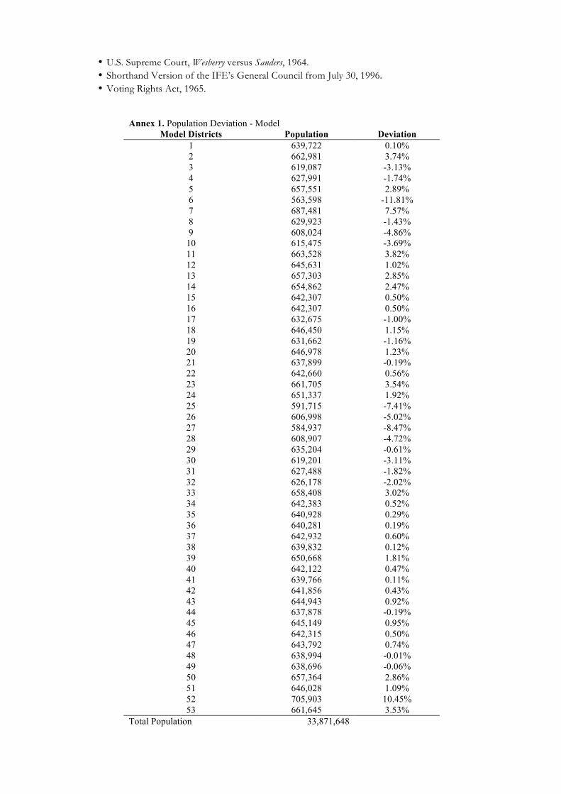
• U.S. Supreme Court, Wesberry versus Sanders, 1964. • Shorthand Version of the IFE’s General Council from July 30, 1996. • Voting Rights Act, 1965.

Annex 1. Population Deviation - Model Model Districts Population Deviation

1 639,722 0.10% 2 662,981 3.74% 3 619,087 -3.13% 4 627,991 -1.74% 5 657,551 2.89% 6 563,598 -11.81% 7 687,481 7.57% 8 629,923 -1.43% 9 608,024 -4.86%

10 615,475 -3.69% 11 663,528 3.82% 12 645,631 1.02% 13 657,303 2.85% 14 654,862 2.47% 15 642,307 0.50% 16 642,307 0.50% 17 632,675 -1.00% 18 646,450 1.15% 19 631,662 -1.16% 20 646,978 1.23% 21 637,899 -0.19% 22 642,660 0.56% 23 661,705 3.54% 24 651,337 1.92% 25 591,715 -7.41% 26 606,998 -5.02% 27 584,937 -8.47% 28 608,907 -4.72% 29 635,204 -0.61% 30 619,201 -3.11% 31 627,488 -1.82% 32 626,178 -2.02% 33 658,408 3.02% 34 642,383 0.52% 35 640,928 0.29% 36 640,281 0.19% 37 642,932 0.60% 38 639,832 0.12% 39 650,668 1.81% 40 642,122 0.47% 41 639,766 0.11% 42 641,856 0.43% 43 644,943 0.92% 44 637,878 -0.19% 45 645,149 0.95% 46 642,315 0.50% 47 643,792 0.74% 48 638,994 -0.01% 49 638,696 -0.06% 50 657,364 2.86% 51 646,028 1.09% 52 705,903 10.45% 53 661,645 3.53%

Total Population 33,871,648

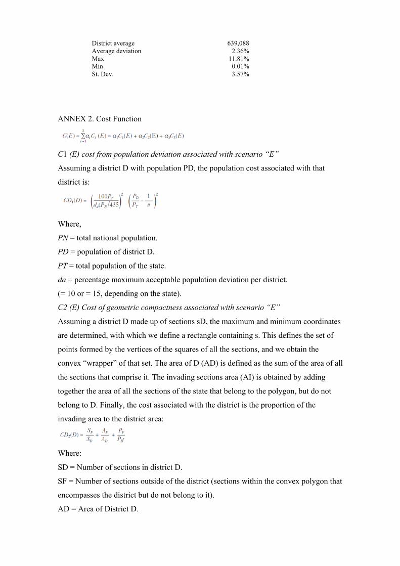
District average 639,088 Average deviation 2.36% Max 11.81% Min 0.01% St. Dev. 3.57%

ANNEX 2. Cost Function

C1 (E) cost from population deviation associated with scenario “E”

Assuming a district D with population PD, the population cost associated with that

district is:

Where,

PN = total national population.

PD = population of district D.

PT = total population of the state.

da = percentage maximum acceptable population deviation per district.

(= 10 or = 15, depending on the state).

C2 (E) Cost of geometric compactness associated with scenario “E”

Assuming a district D made up of sections sD, the maximum and minimum coordinates

are determined, with which we define a rectangle containing s. This defines the set of

points formed by the vertices of the squares of all the sections, and we obtain the

convex “wrapper” of that set. The area of D (AD) is defined as the sum of the area of all

the sections that comprise it. The invading sections area (AI) is obtained by adding

together the area of all the sections of the state that belong to the polygon, but do not

belong to D. Finally, the cost associated with the district is the proportion of the

invading area to the district area:

Where:

SD = Number of sections in district D.

SF = Number of sections outside of the district (sections within the convex polygon that

encompasses the district but do not belong to it).

AD = Area of District D.

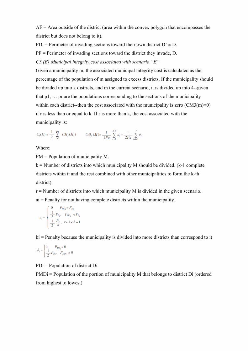
AF = Area outside of the district (area within the convex polygon that encompasses the

district but does not belong to it).

PD, = Perimeter of invading sections toward their own district D’ ≠ D.

PF = Perimeter of invading sections toward the district they invade, D.

C3 (E) Municipal integrity cost associated with scenario “E”

Given a municipality m, the associated municipal integrity cost is calculated as the

percentage of the population of m assigned to excess districts. If the municipality should

be divided up into k districts, and in the current scenario, it is divided up into 4--given

that p1, … pr are the populations corresponding to the sections of the municipality

within each district--then the cost associated with the municipality is zero (CM3(m)=0)

if r is less than or equal to k. If r is more than k, the cost associated with the

municipality is:

Where:

PM = Population of municipality M.

k = Number of districts into which municipality M should be divided. (k-1 complete

districts within it and the rest combined with other municipalities to form the k-th

district).

r = Number of districts into which municipality M is divided in the given scenario.

ai = Penalty for not having complete districts within the municipality.

bi = Penalty because the municipality is divided into more districts than correspond to it

PDi = Population of district Di.

PMDi = Population of the portion of municipality M that belongs to district Di (ordered

from highest to lowest)