1 EDUCATION AND LABOUR MARKET OUTCOMES: EVIDENCE FROM INDIA Aradhna Aggarwal 1 Ricardo Freguglia 2 Geraint Johnes 3 Gisele Spricigo 4 1.National Council of Applied Economic Research, India; [email protected] 2.Federal University of Juiz de Fora, Juiz de Fora, Minas Gerais, Brazil; [email protected] 3.Lancaster University Management School, Lancaster, UK; [email protected] 4.Universidade do Vale do Rio dos Sinos, Porto Alegre, Rio Grande do Sul, Brazil; [email protected] ABSTRACT The impact of education on labour market outcomes is analysed using data from various rounds of the National Sample Survey of India. Occupational destination is examined using both multinomial logit analyses and structural dynamic discrete choice modelling. The latter approach involves the use of a novel approach to constructing a pseudo-panel from repeated cross-section data, and is particularly useful as a means of evaluating policy impacts over time. We find that policy to expand educational provision leads initially to an increased take- up of education, and in the longer term leads to an increased propensity for workers to enter non-manual employment. Keywords: occupation, education, development JEL Classification: I20, J62, O20 While retaining full responsibility for the contents of this paper, the authors gratefully acknowledge support from the Economic and Social Research Council (grant RES-238-25- 0014). Thanks, for useful discussions, are also due to participants at the ESRC Research Methods Festival held in Oxford, Juiz de Fora University, Brazil and National Institute of Public Finance and Policy, India.

Welcome message from author
This document is posted to help you gain knowledge. Please leave a comment to let me know what you think about it! Share it to your friends and learn new things together.
Transcript

1
EDUCATION AND LABOUR MARKET OUTCOMES: EVIDENCE FROM INDIA
Aradhna Aggarwal1
Ricardo Freguglia2
Geraint Johnes3
Gisele Spricigo4
1.National Council of Applied Economic Research, India; [email protected]
2.Federal University of Juiz de Fora, Juiz de Fora, Minas Gerais, Brazil;
3.Lancaster University Management School, Lancaster, UK; [email protected]
4.Universidade do Vale do Rio dos Sinos, Porto Alegre, Rio Grande do Sul, Brazil;
ABSTRACT
The impact of education on labour market outcomes is analysed using data from various
rounds of the National Sample Survey of India. Occupational destination is examined using
both multinomial logit analyses and structural dynamic discrete choice modelling. The latter
approach involves the use of a novel approach to constructing a pseudo-panel from repeated
cross-section data, and is particularly useful as a means of evaluating policy impacts over
time. We find that policy to expand educational provision leads initially to an increased take-
up of education, and in the longer term leads to an increased propensity for workers to enter
non-manual employment.
Keywords: occupation, education, development
JEL Classification: I20, J62, O20
While retaining full responsibility for the contents of this paper, the authors gratefully
acknowledge support from the Economic and Social Research Council (grant RES-238-25-
0014). Thanks, for useful discussions, are also due to participants at the ESRC Research
Methods Festival held in Oxford, Juiz de Fora University, Brazil and National Institute of
Public Finance and Policy, India.
2
1. Introduction
Increased global competition has resulted in rapid changes in the nature of the labour market
in many countries. In developed economies, governments have promoted education as a
means of securing a comparative advantage in the production of goods and services whose
production is knowledge-intensive. Elsewhere, experience has varied, with some developing
countries likewise heading toward an industry mix that places a premium on human capital.
In some measure this is due to the growth in demand for education – an income elastic
product – as incomes rise. It is particularly instructive to examine these issues in the context
of the BRIC countries – Brazil, Russia, India and China – since these are developing rapidly
and offer some contrasting stories.
In India, educational provision, particularly at tertiary level, has expanded rapidly over the
last decade and a half. The enhanced skills with which many young people now enter the
labour force are likely to impact upon their trajectory through the labour market. In particular,
we might expect an increasing proportion of workers to find employment in higher status
occupations. Yet at this stage little is known about precisely how educational policy affects
occupational outcomes in this large country, where the pace of development has been uneven
across sectors (Johnes, 2010).
This paper proposes to assess the impact of education policy on labour market outcomes by
estimating both static and dynamic models of occupational choice using educational
attainment and other individual characteristics as explanatory variables. It does so using the
National Sample Surveys’ data spanning over the period from 1993-94 to 2005-06.
The rest of the paper is structured as follows. We begin with a brief discussion of changes in
India’s education policy since 1990, in Section 2. Section 3 briefly reviews the pertinent
literature on the subject matter. Section 4 discusses the statistical models, both static and
dynamic. Section 5 is a short methodological section. Section 6 describes the dataset,
followed by a presentation of the results of our estimation exercises in Section 7. The paper
ends with a discussion and conclusion provided in Section 8.
2. Education Policy in India: A brief overview of changes since 1990
Since independence, education has been in prime focus in India. Efforts to expand access and
quality of education have characterised successive Five Year Plans. In the period from 1951-
52, when the country launched its first five year plan, until 1990, the number of schools
increased more than three-fold, outpacing the growth of the school age population
(Dougherty and Herd 2008). At the tertiary level, the number of universities rose 7-fold,
while the number of undergraduate and professional colleges rose 10-fold. During this period,
the public expenditure on education also registered a phenomenal growth. It rose several
folds from mere INR 14493.0 million to INR 400198.6 million at constant prices and its
share in GDP increased from 0.6% of GDP in 1950-51 to 3.9% of GDP in 1989-90
In 1991, India embarked on a comprehensive economic reforms programme aiming to
achieve rapid economic growth by integrating the economy with the global economy. This
process created multiple opportunities but it also posed many challenges. The government of
India recognised that one of the most crucial prerequisites to take advantage of the emerging

3
opportunities is human development and that it was directly linked to expansion in education.
This period also witnessed, following the Jomtien World Declaration (1990) on Education for
All (EFA), heightened international pressures to achieve universal access to education within
the shortest possible time frame. In 1992, the government updated the National Policy on
Education to include several key strategies to achieve the goal of universal access to
education and improved school environment. Under this policy, a District Primary Education
Programme was launched as a major initiative to expand people’s participation in education.
In 2000, the government signed Dakar and UN Millennium declarations and reaffirmed its
commitment to education for all. Following this, in 2002, the government unveiled its
national flagship program, the Sarva Shiksha Abhiyan (SSA), to enrol all 6–14 year-olds in
school by 2010. In the same year, free and compulsory education was made a Fundamental
Right for all the children in the age-group of 6-14 years through the 86th Amendment of the
Constitution. While the focus had been on achieving universal education, sweeping reforms
were introduced to broaden access to higher education as well. This led to a proliferation of
private institutions, and also of distance education programmes and self financing
programmes by public institutions. In 2000, 100% FDI was allowed in higher education
under the automatic route. As a result, foreign institutions started offering programmes either
by themselves or in partnership with Indian institutions. This period also witnessed the
growth of the non-university sector. There was rapid expansion of polytechnics and industrial
training institutes, largely in the private sector (Agarwal, 2006).
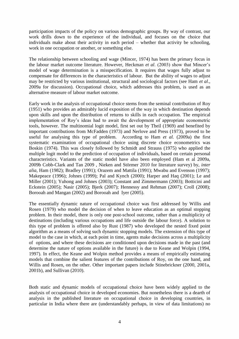
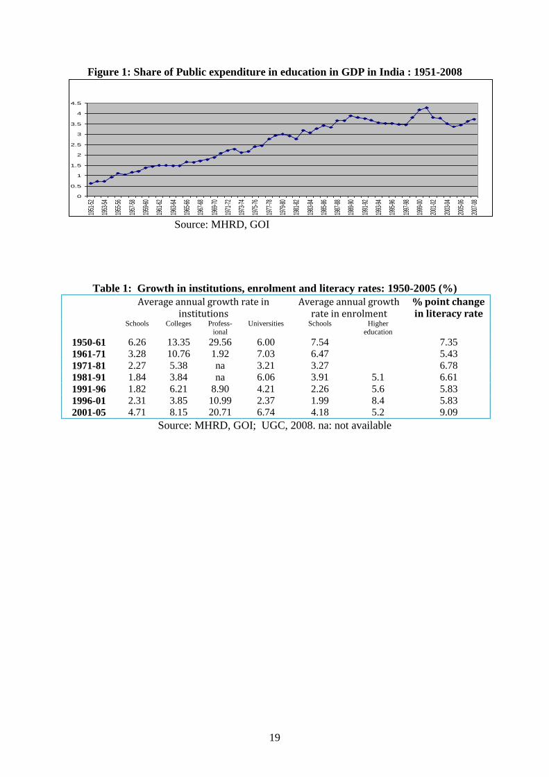
Table 1 shows that the country has made significant strides in quantitative terms. The
expansion of the tertiary sector seems to be the most impressive though. Nonetheless, there
are concerns that the performance of the educational system was not as good as might be
expected, due to resource constraints. Despite higher allocations to education by the centre as
part of implementing the programme with external assistance the public expenditure on
education as a percentage of GNP declined steeply in the early 1990s and touched 3.53 per
cent in 1997-98. In the late 1990s, it started rising again and gained momentum to reach as
high as 4.38 per cent in 2000-01 but this momentum could not be sustained further and the
public expenditure as per cent of GNP plummeted to 3.56 per cent in 2003-04 to rise slowly
once again thereafter. The trends in the share of public expenditure on education as a
percentage of total budget expenditure display a similar pattern. The share of public
expenditure on education in the total budget was 14.0 per cent in 1990-91. But it declined to
13.1 per cent in 1991-92 and was hovering a little over 13 per cent till 1997-98. Though it
increased to 14 per cent in 1998-99 and further to 16.1 per cent in 2000-01, it swiftly declined
to 12.0 per cent in 2003-04 with a slow rise since then.
The 11th
Plan placed education, particularly vocational and science education, at the centre of
development and is termed “Education Plan (2007-2010)”. In nominal terms, it proposed a
five-fold increase in spending on education and pledged to raise public expenditure on
education to 6 percent of total GDP. This is an unprecedented increase in financial support
for education in India. We analyse here how increased public expenditure can influence the
labour market outcome in terms of occupational choice.
3. Literature review
In many respects, an obvious antecedent of the work undertaken in the present paper is a
contribution by Duflo (2004) who examines the impact of a policy decision rapidly to expand
the education sector in Indonesia. Duflo’s work focuses on the wage and labour market
4
participation impacts of the policy on various demographic groups. By way of contrast, our
work drills down to the experience of the individual, and focuses on the choice that
individuals make about their activity in each period – whether that activity be schooling,
work in one occupation or another, or something else.
The relationship between schooling and wage (Mincer, 1974) has been the primary focus in
the labour market outcome literature. However, Heckman et al. (2003) show that Mincer’s
model of wage determination is a misspecification. It requires that wages fully adjust to
compensate for differences in the characteristics of labour. But the ability of wages to adjust
may be restricted by various institutional, structural and sociological factors (see Ham et al.,
2009a for discussion). Occupational choice, which addresses this problem, is used as an
alternative measure of labour market outcome.
Early work in the analysis of occupational choice stems from the seminal contribution of Roy
(1951) who provides an admirably lucid exposition of the way in which destination depends
upon skills and upon the distribution of returns to skills in each occupation. The empirical
implementation of Roy’s ideas had to await the development of appropriate econometric
tools, however. The multinomial logit model, first set out by Theil (1969) and benefited by
important contributions from McFadden (1973) and Nerlove and Press (1973), proved to be
useful for analysing this type of problem. According to Ham et al. (2009a) the first
systematic examination of occupational choice using discrete choice econometrics was
Boskin (1974). This was closely followed by Schmidt and Strauss (1975) who applied the
multiple logit model to the prediction of occupation of individuals, based on certain personal
characteristics. Variants of the static model have also been employed (Ham et al 2009a,
2009b Cobb-Clark and Tan 2009 , Nieken and Störmer 2010 for literature survey) by, inter
alia, Ham (1982); Bradley (1991); Orazem and Mattila (1991); Mwabu and Evenson (1997);
Makepeace (1996); Johnes (1999); Pal and Kynch (2000); Harper and Haq (2001); Le and
Miller (2001); Yuhong and Johnes (2003); Constant and Zimmermann (2003); Botticini and
Eckstein (2005); Nasir (2005); Bjerk (2007); Hennessy and Rehman (2007); Croll (2008);
Borooah and Mangan (2002) and Borooah and Iyer (2005).
The essentially dynamic nature of occupational choice was first addressed by Willis and
Rosen (1979) who model the decision of when to leave education as an optimal stopping
problem. In their model, there is only one post-school outcome, rather than a multiplicity of
destinations (including various occupations and life outside the labour force). A solution to
this type of problem is offered also by Rust (1987) who developed the nested fixed point
algorithm as a means of solving such dynamic stopping models. The extension of this type of
model to the case in which, at each point in time, agents make decisions across a multiplicity
of options, and where these decisions are conditioned upon decisions made in the past (and
determine the nature of options available in the future) is due to Keane and Wolpin (1994,
1997). In effect, the Keane and Wolpin method provides a means of empirically estimating
models that combine the salient features of the contributions of Roy, on the one hand, and
Willis and Rosen, on the other. Other important papers include Stinebrickner (2000, 2001a,
2001b), and Sullivan (2010).
Both static and dynamic models of occupational choice have been widely applied to the
analysis of occupational choice in developed economies. But nonetheless there is a dearth of
analysis in the published literature on occupational choice in developing countries, in
particular in India where there are (understandably perhaps, in view of data limitations) no
5
dynamic studies, and static analyses are also hard to come by. Khandker (1992) uses survey
data from Bombay to evaluate earnings and, using multinomial logit methods, occupational
destination of men and women. This study uncovers evidence of labour market segmentation.
More recently, Howard and Prakash (2010) have likewise used multinomial logit methods,
and find, using data from the National Sample Survey, that the imposition of quota policies
on the employment of scheduled caste and scheduled tribes in public sector jobs has had a
positive effect on the occupational outcomes for these socially backward groups. In a recent
study, Singh (2010) used the India Human Development Survey, 2005 data and found that the
individuals with higher education and better ability are more likely to be government (and
permanent) employees. There is thus no comprehensive analysis of how educational
attainment impacts on occupational outcomes of young workers entering the labour market in
India and how this link is influenced by public expenditure on education.
4. Theoretical framework and statistical modelling
There are various explanations offered in the literature for heterogeneity in individuals’
occupational outcomes (Levine 1976, Ham et al. 2009a, 2009b). One explanation that is most
predominantly used in labour economics is human capital theory (Becker 1964, Benewitz and
Albert Zucker, 1968, Boskin 1974). The human capital theory is focused on the effects of
education, experience and an individual’s innate ability in determining their productivity in
various tasks and returns from their labour (Becker, 1964). It has been extended to develop a
model of occupational choice centered on the preferences of individuals for particular time
shapes of their income streams (Benewitz and Albert Zucker, 1968, and Boskin, 1974). The
occupational choice in this framework is the result of a process taking place over a period of
many years in a sequence of investment activities undertaken for entry into an occupation.
This sequence, described by Benewitz and Albert Zucker (1968), is an ordered chain each
part of which has a rate of return associated with it. An individual must decide at each step of
this chain whether to stop further investment in human capital or to go on. If she stops then
she is likely to enter a lower investment occupation than if she continues. Thus educational
attainment and occupation choice are endogenously determined. A worker chooses that career
path for which the present value of her discounted income stream is a maximum. The
discount rate is determined by the time preference function which in turn depends on the
quality of education, direct and opportunity cost of education, age, sex and other socio-
economic characteristics. Public investment impinges on the individual’s time preference
function by influencing both direct cost and quality of education.
Boskin (1974) applied the conditional logit decision model to the choice of occupation by
individual workers. He showed that decisions on occupational choice are governed by the
returns-primarily expected potential (full-time) earnings-and costs of training and foregone
potential earnings. Using this framework we estimate a reduced-form Mincer type
specification for occupational choice:
Yi = f (Si, Xi) + ui (1)
where Yi is a measure of labour market outcome, Si is the schooling of the ith individual, and
Xi contains other individual characteristics; ui is a random error. This equation is estimated
by an appropriate technology - where Y is a limited dependent variable indicating
occupational destination. In static terms, logit or probit methods are commonly used to
estimate this relationship while the dynamic analysis is based on dynamic discrete choice
6
models. Note that this is then a reduced form approach – we do not explicitly model
earnings, but the vector of characteristics on the right hand side of the equation themselves
are deemed to influence earnings as well as the outcome of interest.
In the literature, there are various attempts to classify occupations. These include and are not
limited to: social status based ranking systems (Jones and McMillan 2001; Lee and Miller
2001); Holland’s six occupational types (Larson et al. 2002; Porter and Umbach 2006;
Rosenbloom et al. 2008); the ranking of occupations by skill – unskilled, semi-skilled,
skilled, etc. (Darden 2005); good jobs and bad jobs (Mahuteau and Junankar 2008); and blue
and white collared jobs (Ham et al., 2009a).
We consider six labour market outcomes for our dependent variable: (i) not in work or
schooling; (ii) in education; (iii) manual employees; (iv) manual self-employed workers; (v)
non-manual employees; and (vi) non-manual self-employed workers.
Turning to the explanatory variables we use schooling years for educational attainment. In the
Mincerian type version, Si is simply years of education, representing a linear relationship
between years of education and occupational choice. We include, in a further specification,
also a quadratic term in years of education to capture variations in the relationship between
education and earnings. Most studies in the Indian context have found returns to schooling
heterogeneous (Duraiswamy 2002, Dutta 2006). In general, heterogeneous returns to
education for wage workers have been found by, for instance Heckman et al. (2006) and
Iversen et al. (2010)
As additional controls, we use a range of socio-demographic variables: age, age squared,
religion (Islamic, Christian, other), gender, social group, household land holdings (in
hectares), and household literacy rate. Age proxies potential years of experience, since we do
not have data on actual years of experience. Social group is a dummy for people belonging to
scheduled tribe and scheduled caste and are considered socially backward. Religion is
represented by dummy variables for three categories of minorities such as Islam, Christianity
and other religions (where Hindus, the majority group, form the excluded category). A large
body of literature has investigated parental influence on occupational choice using the
available information (Nieken and Störmer, 2010). These factors affect outcomes by both
influencing the productive capabilities and the preferences of an individual. We have
incorporated here land ownership and family literacy rate as proxies for household wealth
and education. Differences by gender are captured by a dummy for males. Finally, aggregate
effects mask vast regional variations. These are captured by incorporating regional dummies.
Long run factors such as government policies can systematically change labour markets and
hence also the occupational choices of all individuals. These are controlled by estimating the
static model for three different years. The models are estimated for the 15-35 age; we have
also run the models on the 23-35 age group as a robustness check, but since the results are
generally similar to those obtained for the 15-35 group, we do not report them here.
5. Methodology
(i) Static model
The static model involves the use of maximum likelihood methods to choose the appropriate
parameter estimates in the expressions
7
P(Y=j) =
, j=1,2,...,J
P(Y=0) =
(2)
where the δ terms are parameters and the z are the explanatory variables.
The multinomial logit method, while instructive, does suffer some drawbacks. The first, well
documented in the literature, is that it makes an assumption of the independence of irrelevant
alternatives. That is, it is assumed that the relative odds between two alternative outcomes are
unaffected by augmenting the set of possible outcomes. In some contexts – particularly where
the qualitative characteristics of the added regime are close to one but not the other of the two
alternatives under study – this assumption is clearly absurd. Several partial fixes for this
problem have been suggested in the literature, including nested logit and mixed logit
methods.1 In the present paper we adopt a different approach – that of dynamic discrete
choice modelling. The dynamic model links theory to empirical application by adopting a
structural approach in which all possible regime choices are included, and, at each date,
experience in each regime determines the instantaneous returns to each regime.
A second, rather obvious, feature of the static multinomial logit analysis that is unappealing
in the present context is that it is poorly equipped to investigate the impact of policy changes.
In particular, the long term impact of an instantaneous change in education policy – where
education is usefully regarded as an investment in an individual’s future labour market
performance – is not readily captured in a static analysis. For this reason too, use of a
dynamic approach is appealing.
(ii) Dynamic discrete choice model
The dynamic analysis is based on Keane and Wolpin (1997). The essence of the problem
identified by Keane and Wolpin is very simple. In each period, individuals choose between
activities. The instantaneous return to each activity depends upon past experience which is
made up of the schooling and labour market choices that the individual has made in the past.
In each period the choice made by the individual therefore impacts on the returns that she can
make not only in that period but in every subsequent period. For an individual seeking to
maximise her lifetime returns, the state space is therefore huge. Empirical evaluation of such
a model requires the adoption of approximation methods. Keane and Wolpin propose the
evaluation of expected future returns at a sample of points in the state space, fitting a
regression line on the basis of this sample, and using this line to estimate expected future
returns for points outwith the sample. Using these estimates allows us then to proceed to
estimate the parameters of the model in the usual way, using maximum likelihood. We use
the variant of the Keane and Wolpin model that allows for regime-specific shocks to be
serially correlated.
1 Soopramanien and Johnes (2001) offer an example of the use of such methods in the context of occupational
choice.

8
A feature of the structural modelling approach used here is the close relationship between the
theoretical model and the empirical implementation. The analyst begins with an assumed
specification of the model, and estimates this model.2 For this reason, empirical applications
of this kind are often referred to as structural models.
In this section we evaluate the dynamic model, taking seriously the starting point provided by
Keane and Wolpin. The data allowed us a crude occupational classification to be made. We
classify employers and regular salaried or waged employees as ‘high status occupations’, and
own account workers, casual wage labour in public works, and other types of work as ‘low
status occupations’. The usual primary status variable also has a code for respondents who
are ‘in education’, which defines our schooling indicator.3 Other codes for the usual primary
status variable are taken to represent activity other than work or education.
We thus begin with the following instantaneous reward functions:
R1t = α10+α11st+α12x1t+α13 x2t+ε1t
R2t = α20+α21st+α22x1t+α23 x2t+ε2t
R3t = β0+β1I(st12)+β2educpol+ε3t
R4t = γ0+ε4t (3)
Here s refers to years of schooling received prior to the current period t, x1 is years of
experience in occupation 1, and x2 is years of experience in occupation 2. The terms R1
through R4 denote respectively the instantaneous returns to working in occupation 1 (high
status occupations), occupation 2 (low status occupations), or schooling, or other activity
(which may include other work, unemployment, or absence from the labour force). We do not
observe individual specific wages in the data, and this is a point of contrast between the
present exercise and the model estimated by Keane and Wolpin. Nevertheless, the parameters
of the model can be estimated, albeit with a restriction that we introduce later. The ε terms
represent alternative-specific, period-specific, random shocks. These are crucial in
determining why some workers take certain paths through their career while others take
others. The first term in the instantaneous reward for schooling equation indicates that we
expect the one-period ‘reward’ associated with schooling at tertiary level, β1, to be negative
owing to the payment of tuition fees. The second term in that equation is intended to capture
the effect of education policy (educpol) on the decision to stay on at school, and the sign and
magnitude of the coefficient attached to that variable, β2, is therefore of primary interest in
the present study. To ensure identification of the model, we impose γ0= ε4t =0. Education
policy is measured as the percentage of GDP that comprises public spending on education.
These data are available from the Ministry of Human Resource Development Figure 1.
While attractive in the sense that this approach involves the estimation of the parameters of
the theoretical model itself, there are some disadvantages. First, a reader might wish to
quibble with the precise specification being assumed in the theoretical model; since the
empirical implementation is so closely linked to that particular specification, such a quibble
2 This contrasts with more usual practice, which is to develop some theory and then use regression analysis to
test whether or not a particular variable influences another in a particular direction consistent with that theory. 3 Since we need our panel to follow individuals through the point at which they enter the labour market, and
since the statutory school leaving age is 14, we assume that individuals aged 14 and under are in education,
regardless of whether or not the usual primary status variable indicates that they are otherwise occupied.
9
assumes empirical importance. Secondly, the close link between theory and estimation means
that generic software cannot be developed to estimate models of this kind. In effect, the
whole program must be rewritten from scratch each time the specification of the model is
subject to a minor modification. These issues have been widely discussed in the literature.
Keane (2010), for example, has noted that ‘structural econometric work is just very hard to
do’ – and so is not fashionable. We recognise this; we invite the reader therefore to go along
with our story while appreciating that no small aspect of the story can be easily tweaked.
In one important respect, our task has been easier than that of earlier researchers in this area.
A recent survey of structural dynamic discrete choice models by Aguirregabiria and Mira
(2010) is accompanied by a website4 that offers software that has been used by earlier
researchers to estimate these models.5 The software is written in high level languages (the
Keane and Wolpin program, for example, is in fortran), and requires considerable adaptation
before being used to estimate even models that are very similar to those evaluated in the
original applications. It nevertheless provides a useful starting point.
6. Data
Multinomial logit models
The parameters of the static models are estimated using quinquennial rounds (although this
description is rather imprecise) of National Sample Surveys on employment and
unemployment at three points in time spanning more than a decade: 1993-94, 1999-2000 and
2005-06. The analysis permits us to compare the relationship between educational attainment
and occupational choice across three points in time. These surveys contain particularly rich
data on occupation and educational attainment at the level of the individual. These surveys
also collect a wide array of data on the socio-economic characteristics of individuals
including, religion, age, caste, and land possessed. Occupations are defined from an
individual's primary labor market status and are available at three-digit NCO classification.
The 1993-94 Survey consists of 115,409 households containing 564,740 individuals , while
1999-2000 and the 2005-06 rounds have 165052 households representing 819013 individuals
and 78,879 households with 413,657 individuals, respectively.
Dynamic models
For dynamic models we use data from the annual NSS surveys on per capita expenditure
over the period 1995-20066. In essence, these surveys are conducted to provide information
on per capita expenditure but they also provide rich information on the age, gender, activity
status, and educational attainment of individuals. The NSS is a large cross-section data set,
repeated each year but with a different sample of individuals.7 In order to use these data in the
context of a dynamic analysis, it is therefore necessary first to construct a synthetic panel.
4 http://individual.utoronto.ca/vaguirre/wpapers/program_code_survey_joe_2008.html
5 Another useful recent survey is provided by Keane and Wolpin (2009).
6 These are rounds 51 through 62.
7 While there do exist panel data sets for India, these are not suitable for the present analysis since they do not
provide individuals’ work histories in the form of regularly collected data over a lengthy period. The Rural
Economic and Demographic Survey (REDS) data followed on from the Additional Rural Income Survey of the
late 1960s. REDS comprises four sweeps, taken in 1970-71, 1982, 1999 and 2006. The sweeps clearly do not
10
Deaton (1985) showed that, under reasonable assumptions, it is possible to construct a
pseudo-panel from repeated cross sections. This simply involves constructing cohorts of
individuals in each year, based on their age and other characteristics, and then using the
cohort average values of all variables across the repeated cross sections. This collapses a
large number of observations into a pseudo-panel comprising a smaller number of synthetic
observations. Moffitt (1993) showed that this method is tantamount to the adoption of an
instrumental variables approach in which the instruments comprise a full set of cohort
dummies. Earlier attempts at constructing pseudo-panels using NSS data include Imai and
Sato (2008).
In the present context, the traditional approach to constructing a pseudo-panel is not available
to us. This is because using the cohort mean values of characteristics such as occupation or
attendance at school would result in non-integer values that do not make sense in the dynamic
discrete choice framework.8 We therefore construct a synthetic panel by matching individuals
from the last sweep of the survey with individuals from the previous sweep, then matching
individuals from the latter sweep with individuals from the sweep before, and so on until a
complete panel is constructed. The matching is done using the nearest neighbour, based on
propensity score, without replacement. Matching is on age and region.9 Region is defined by
six broad regions plus a miscellaneous category – the regions are: North West (Himanchal
Pradesh, Jammu and Kashmir, Uttaranchal); North Central (Bihar, Haryana, Madhya
Pradesh, Punjab, Uttar Pradesh, Delhi); West (Goa, Gujarat, Maharashtra, Rajasthan); East
(Chhattisgarh, Jharkhand, Orissa, Sikkim, West Bengal); South (Andhra Pradesh, Karnataka,
Kerala, Tamil Nadu); and North East (Arunachal Pradesh, Assam, Manipur, Meghalaya,
Mizoram, Nagaland, Tripura). The use of matching methods to produce a synthetic panel in
this way likely produces more switching (from year to year) of destination status than would
be observed in a true panel; any bias that this introduces into the estimation is unavoidable.
In view of the large size of this data set, and of the computer intensive nature of the
estimation procedure being used, we have taken a random sample of 5000 male workers, all
of whom pass through the school leaving age of 14 at some point during the 1995-2006
window. To operationalise the selection of observations, 5000 males were chosen at random
out of the 2006 data, and these were matched with males drawn from the full set of
observations for the earlier years. We do not include females in our dynamic analysis because
the richer array of outcomes that is characteristic of women would add considerable
complexity to a modelling exercise that is already challenging.
take place frequently enough to provide complete work histories. Further panel data are offered by the India
Human Development Survey (IHDS), but again the sweeps are limited in number and are more than a decade
apart (1993-4 and 2005-6). An early study that uses the IHDS is that of Singh (2010). 8 Collado (1997, 1998) and Verbeek (2008) have considered the issue of pseudo-panels in the context of limited
dependent variable models that are static in nature, but unfortunately their approach cannot be used in the
dynamic context. 9 We considered including other variables. In particular, educational attainment was considered, but proved to
be problematic, since many in our sample are at an age where their educational attainment is changing; an
individual aged, say, 26 in 2006 may have completed higher education, but in 1995 such an individual can only
have completed compulsory education and is therefore indistinguishable from other respondents of the same
age. Clearly results from the analysis that follows may be sensitive to the choice of both matching technology
and the variables (and, for that matter, the level of aggregation used in defining variables such as region) used
for matching.
11
7. Empirical results
We report the results of our statistical models by considering, first, the static multinomial
logit specification, and, later, the dynamic discrete choice model.
Multinomial logit models
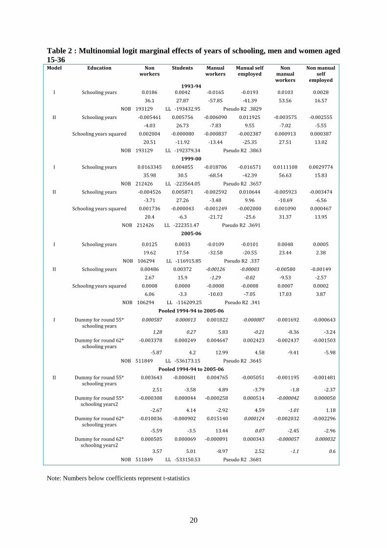
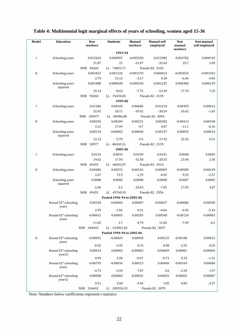
In Tables 2-4, we report the marginal effects of the years of schooling variables, separately
for each year, and separately for males, females, and all respondents along with the results of
an analysis in which data from all three rounds are pooled, but the schooling variables are
interacted with a round index so that we can investigate how the impact of schooling has
changed over time. Model 1 is our benchmark version with a linear term for schooling years
while Model II includes a quadratic term for the schooling variable. For reasons of space, we
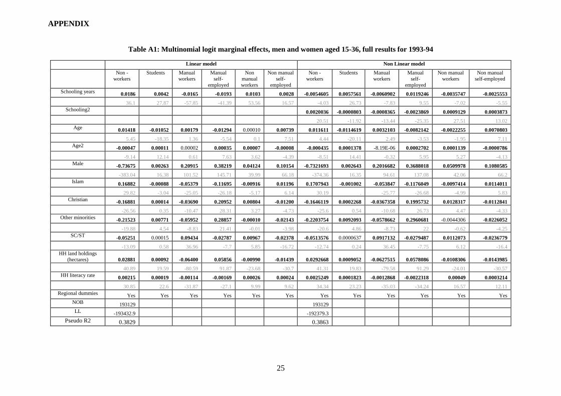
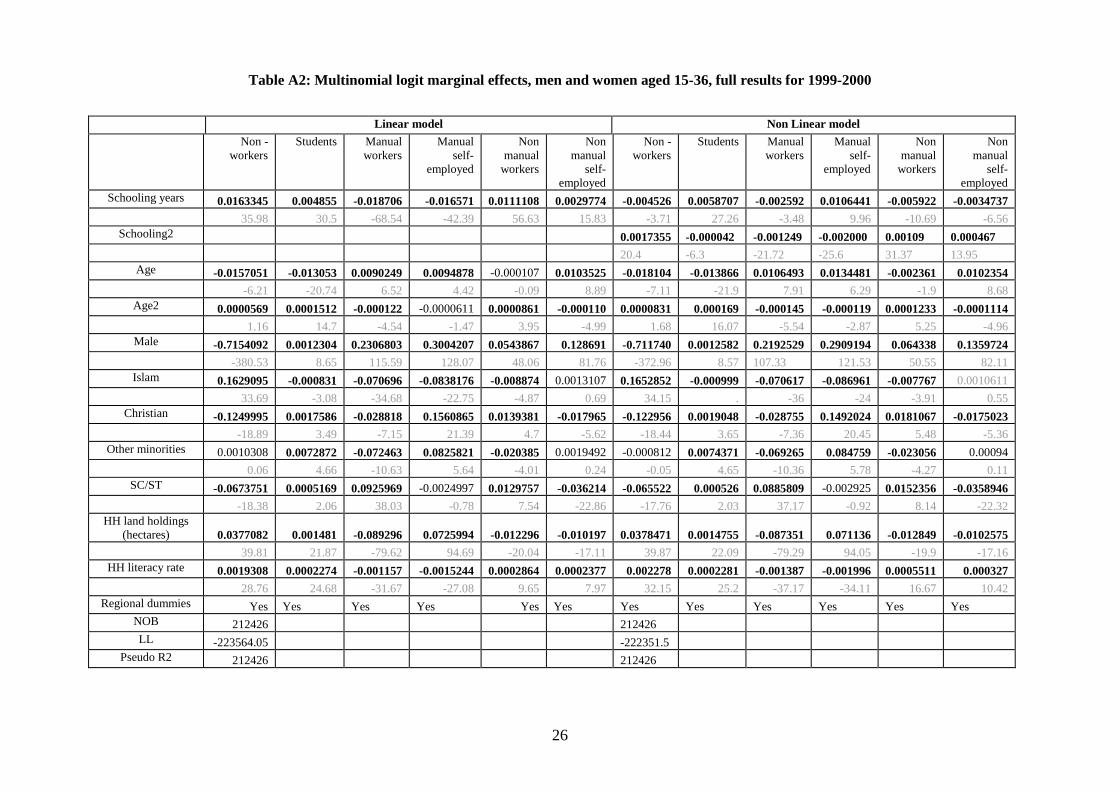
do not report the marginal effects of the other variables in full; we do, however, report the
results, pooled across men and women, for a typical year in the appendix.
It is clear from our linear version of the model that in all years, schooling raises the probability with
which an individual enters non-manual work, and reduces the probability with which an individual
enters manual work. Schooling also raises the probability of continuing in education and –
more surprisingly, perhaps – of being in neither work nor schooling. These results hold across
both genders, but the marginal effects associated with the impact of schooling on
occupational choice are greater for males than for females (Tables 3 and 4).
Men are more likely to be in work or schooling than are women. Workers in scheduled tribe
and scheduled castes are more likely to be employed, and less likely to be self-employed,
than other workers. They are also more likely to be in education. Clearly, the imposition of
quota policies has had a positive impact not only on job selection among socially backward
classes as shown by Howard and Prakash (2010) but also on education. There seems to be a
systematic relationship between religion and occupational choice. While Muslims are more
likely to be in non-manual self-employment, Christians exhibit greater probability of entering
into manual self-employment than Hindus. Our findings are in line Audretsch et al. (2007)
who found Islam and Christianity to be conducive to entrepreneurship, while Hinduism
appears to inhibit entrepreneurship. Parental variables emerge as significant in nearly all
specifications. Individuals resident in households with substantial holdings of land are
relatively likely to be engaged in self-employed manual work; presumably this often takes the
form of farming while those from educated families are more likely to attain higher education
and take up non-manual occupations.
Unsurprisingly, the propensity to be in higher education increases over time after controlling
for unobserved time varying effects (through time specific dummy variables) for both the age
ranges considered here. There is thus evidence of changes in individuals’ time preference
function with more time allocated to education. But contrary to our expectations, the
marginal effects of schooling on the probability of entering manual work increased over time
from 1993-94 through 2004-05 while those on adopting non manual work declined.
We estimated a non linear relationship to further probe this relationship. In model II, both
linear and quadratic terms for schooling years become highly significant while all other
parameter estimates remain largely unaffected. This provides strong evidence of non-linear
effects of education on occupational choice. In the linear model each extra year of schooling
increases the probability of being a non-worker. But Model II indicates that the probability of
12
being neither in education nor in employment first declines with education but then increases
after a threshold level of education. Interestingly these job market patterns seem to have been
reinforced over time through the 1990s and early 2000s but weakly. In 2005-06, the
incremental effect of higher education on the probability of being non worker or non student
was negative when compared with 1999-00. Reforms in higher education during this period
appear to have paid off in terms of more employment opportunities for individuals with
higher education. Further, the probability of continuing education also increases at lower
levels of income but is reversed at higher levels of education. Over time, these patterns also
became more pronounced. In all the specifications, the probability of taking up manual jobs
or manual self employment is negatively associated with higher education and is positive for
non manual jobs and self employment. However, we observe some interesting changes in
these patterns, in particular in the 2005-06 survey results. While manual jobs are increasingly
disliked by the people with higher education, it does not necessarily translate into preference
for non-manual jobs. Rather, we observe increasing preference for self-employment both
manual and non-manual. The present system of higher education has been criticized for being
too academic and biased toward literary subjects thus encouraging passive receptivity (GOI,
1972). These incremental changes signal positive developments in the labour market
outcomes of education reforms. Interestingly, these changes are more obvious for males than
females (Tables 3-4). An important caveat to these results is that marginal effects of the
observed variables are constrained to equality across occupation groups.
In order to check the robustness of the above results, however, we estimated the model with a
different age group 23-35. The results presented above are found to be robust to a different
choice of the age group. Further, the results are also robust to the model specification; the
inclusion of a quadratic term yields more information without affecting the main employment
patterns predicted by the model.
The results reported above make clear that an increased incidence of education raises the
probability with which individuals remain in education (unsurprisingly), and the probability
with which they enter employment as non-manual workers. It is clear therefore that national
investment in education has a direct impact on occupational outcomes, leading to more
workers entering non-manual jobs. It is readily observed that, almost without exception, these
marginal effects are highly significant, and that they affect outcomes in the expected
direction. We investigate this further as we turn to consider the dynamic modelling of
destination.
Dynamic models
As with any approximation method, a number of parameters need to be set by the analyst in
order to proceed. For the simulation used to evaluate the regime that yields the greatest
expected future return, we use 500 draws; we evaluate the expected return at 300 randomly
chosen points in the state space and use the interpolation method for all other points. The
discount parameter is set at 0.95. The convergence toward the maximum likelihood solution
is deemed to be complete when further iterations fail to achieve an improvement in the log
likelihood that exceeds 0.001%.
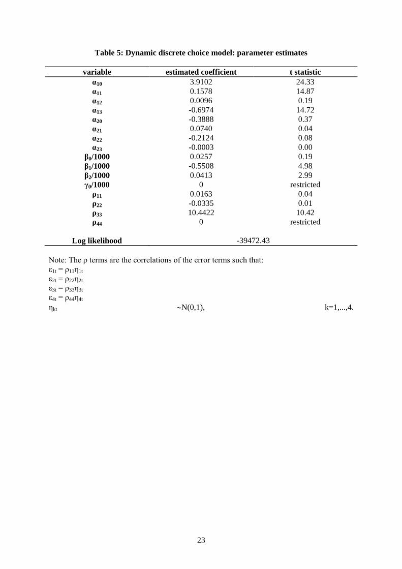
Parameter estimates are reported in Tables 4, and are broadly in line with our prior
expectations. The key finding is that educpol raises the propensity of respondents to stay in
education. Moreover, educational attainment increases the propensity to be in high status

13
occupations relative to lower status occupations; it also increases the propensity to be in work
relative to being neither in work nor in schooling. The high value of the ρ33 parameter
indicates that there is a considerable amount of unobserved heterogeneity across individuals,
and that this impacts on the returns that are available to education; it may be the case that this
could be modelled by separately evaluating coefficients for respondents that come from
different family backgrounds, but this is an exercise that we leave for further work.
Following Keane and Wolpin (1994, 1997) we evaluate standard errors using the outer
product of numerical first derivatives. Keane and Wolpin note that there may be a downward
bias associated with these standard errors. The t statistics reported in Table 4 are high for
many of the coefficients, this being typical of results achieved elsewhere in analyses of this
kind. Moreover, we note that the educpol variable is clustered across all observations in a
given year. We are not aware of any literature that allows correction for such clustering in
this context, but note that this too will likely bias the standard error downwards. Hence our
central result concerning the impact of educational policy needs to be interpreted with some
measure of caution.
It is possible to use the estimates reported in Table 4 as a starting point in an exercise which
aims to evaluate how future changes in educational policy are likely to affect occupational
outcomes. The software provided by Keane and Wolpin includes a program that, given the
estimated parameter values, enables us to compute the within period probabilities with which
a randomly selected observation is expected to appear in each regime in each period of the
time frame under consideration; we can thus calculate these probabilities for an assumed time
series of the educational policy variable. This is, once again, a rather computationally
intensive exercise: for each individual in each period it is necessary to evaluate the expected
lifetime returns at each point in a large state space. We do so using Keane and Wolpin’s
default values. Raising the educational policy variable from 3% to 4% has the effect of
raising the unconditional mean value of years spent in non-manual formal sector work from
1.0900 to 1.0906. The value of these means is small (since many individuals in the sample
are of an age still to be in compulsory education), and the change itself is small, but the
direction of change is very much in line with intuition.
8 Conclusions
An increase in spending on education leads, not surprisingly, to an increase in the propensity
for young people to undertake education. Later in the life cycle, the human capital that they
have acquired equips these young people to undertake jobs that are qualitatively different
from those in which they would otherwise have become employed. Put simply, more people
get better jobs. This should be expected to tilt the economy’s comparative advantage toward
the production of goods and services that are more skill intensive and hence more
remunerative.
Our results are plausible, but should be treated with a measure of caution. The matching
procedure used to construct the synthetic panel is, we think, interesting; but it is an untested
tool. Clearly the results are, to a greater or lesser extent, likely to be sensitive to changes in
the way in which the matching exercise is conducted – matching on a different set of
variables or using a different matching technology may not be innocuous. The need to
construct a pseudo-panel has also driven our decision to limit the time frame under
consideration to just 12 years; a longer panel would introduce greater potential for suspect

14
matches. Unfortunately the only true panel data sets for India are unsuitable for this type of
analysis. The problem considered in this paper shows just how valuable a dataset comprised
of longitudinal data on the labour market experience of individuals in India (whether
collected in real time or by recall) could be.
References
Agarwal, Pawan (2006) Higher education in India: the need for change, ICRIER Working
Paper No. 180, June, New Delhi
Aguirregabiria, Victor and Pedro Mira (2010) Dynamic discrete choice structural models: a
survey, Journal of Econometrics, 156, 38-67.
Audretsch, David B., Bönte Werner and Jagannadha Pawan Tamvada (2007) Religion and
entrepreneurship, Centre for Economic Policy Research Discussion Papers number 6378,
London
Becker, Gary (1964) Human capital; a theoretical and empirical analysis with special
reference to education, National Bureau of Economic Research, New York
Bjerk, David (2007) The differing nature of black-white wage inequality across occupational
sectors.' Journal of Human Resources, 42 (2), 398-434.
Borooah, Vani K. (2001) How do employees of ethnic origin fare on the occupational ladder
in Britian?, Scottish Journal of Political Economy, 48(1), 1-26.
Borooah, Vani K. and Sriya Iyer (2005) The decomposition of inter-group differences in a
logit model: Extending the Oaxaca-Blinder approach with an application to school enrolment
in India. Journal of Economic and Social Measurement, 30 (4), 279
Borooah, Vani K. and John Mangan (2002) An analysis of occupational outcomes for
indigenous and asian employees in Australia. The Economic Record, 78(1), 31-49.
Boskin, Michael (1974) A conditional logit model of occupational choice, Journal of
Political Economy, 82, 389-398.
Botticini, Maristella and Zvi Eckstein (2005) Jewish occupational selection: education,
restrictions, or minorities?, The Journal of Economic History, 65(4), 922-948.
Bradley, Steve (1991) An empirical analysis of occupational expectations. Applied
Economics, 23(7), 1159.
Cobb-Clark, Deborah A. and Michelle Tan, (2009) Noncognitive skills, occupational
attainment, and relative wages, Institute for the Study of Labor (IZA) Discussion Paper 4289,
July, Bonn Germany.
Collado, M. Dolores (1997) Estimating dynamic models from time series of independent
cross-sections, Journal of Econometrics, 82, 37-62.
15
Collado, M. Dolores (1998) Estimating binary choice models from cohort data,
Investigaciones Económicas, 22, 259-276
Constant, Amelie and Zimmermann, Klaus F., (2003) Occupational Choice Across
Generations," IZA Discussion Papers 975, Institute for the Study of Labor (IZA),Bonn
Germany
Croll, Paul (2008) Occupational choice, socio-economic status and educational attainment: a
study of the occupational choices and destinations of young people in the British Household
Panel Survey, Research Papers in Education, 1 (2008), 1 - 26.
Darden, Joe (2005) Black occupational achievement in the Toronto census metropolitan area:
does race matter?, Review of Black Political Economy, 33(2), 31-54.
Deaton, Angus (1985) Panel data from time series of cross-sections, Journal of
Econometrics, 30, 109-126.
Dougherty, Sean and Richard Herd (2008) Improving human capital formation in India,
OECD Economics Department Working Papers, No. 625, OECD Publishing.
Duraisamy, Palanigounder (2002) Changes in returns to education in India, 1983-94: by
gender, age-cohort and location, Economics of Education Review, 21(6), 609-622
Dutta, Puja V. (2006) Returns to education: new evidence for India, 1983–1999, Education
Economics, 14( 4), 431-51, December.
Duflo, Esther (2004) The medium run consequences of educational expansion: evidence from
a large school construction program in Indonesia, Journal of Development Economics, 74,
163-197.
Government of India (1972) Report submitted by the Working group on education
constituted by the expert committee on unemployment, in Virendra Kumar (1988)
Committees and Commissions in India 1971-1973 Vol (II), Taj Press, New Delhi
Ham, John C. (1982) Estimation of a labour supply model with censoring due to
unemployment and employment, Review of Economic Studies, 49, 335-354.
Ham, Roger, Pramod N. Raja Junankar and Robert Wells, (2009) Occupational Choice:
Personality Matters, IZA Discussion Paper 4105, IZA Bonn, Germany. 2009;
Harper, Barry and Mohammad Haq (2001) Ambition, discrimination, and occupational
attainment: a study of a British cohort. Oxford Economic Papers, 53(4), 695-720
Heckman, James, Jora Stixrud and Sergio Urzua (2006) The effects of cognitive and
noncognitive abilities on labor market outcomes and social behavior. Journal of Labor
Economics, 24(3) 411.
Heckman, James J., Lance Lochner and Petra Todd (2003) Fifty years of Mincer earnings
regressions, NBER Working papers, Cambridge, Massachusett
16
Hennessy, Thia C. and Tahir Rehman (2007) An investigation into factors affecting the
occupational choices of nominated farm heirs in Ireland, Journal of Agricultural Economics,
58(1), 61-75.
Howard, Larry L. And Prakash, Nishith (2010) Does employment quota explain occupational
choice among disadvantaged groups? A natural experiment from India, available at
http://works.bepress.com/cgi/viewcontent.cgi?article=1007andcontext=nishithprakash
Imai, Katshushi S. and Sato, Takahiro (2008) Fertility, parental education and development in
India: evidence from NSS and NFHS in 1992-2006, University of Manchester discussion
paper, available at http://papers.ssrn.com/sol3/papers.cfm?abstract_id=1311219.
Iversen, Jens, Nikolaj Malchow-Møller, Anders Sørensen (2010) Returns to schooling in self-
employment, Economics Letters, 109, 179–182
Johnes, Geraint (1999) Schooling, fertility and the labour market experience of married
women, Applied Economics, 31, 585-592.
Johnes, Geraint (2010) It was all gonna trickle down: what has growth in India’s advanced
sectors really done for the rest?, Indian Economic Journal, 57, 146-155.
Jones, Frank L. and Julie McMillan (2001) Scoring occupational categories for social
research: A review of current practice, with Australian examples, Work Employment and
Society, 15( 3),. 539-563.
Khandker, Shahid .R. (1992) Earnings, occupational choice and mobility in segmented labor
markets of India, available at http://www-
wds.worldbank.org/external/default/WDSContentServer/WDSP/IB/1999/10/23/000178830_9
8101903550855/Rendered/PDF/multi_page.pdf
Keane, Michael P. (2010) Structural v atheoretic approaches to econometrics, Journal of
Econometrics, 156, 3-20.
Keane, Michael P. and Wolpin, Kenneth I. (1994) The solution and estimation of discrete
choice dynamic programming models by simulation and interpolation: Monte Carlo evidence,
Review of Economics and Statistics, 76, 648-672.
Keane, Michael P. and Wolpin, Kenneth I. (1997) The career decisions of young men,
Journal of Political Economy, 105, 473-522.
Keane, Michael P. and Wolpin, Kenneth I. (2009) Empirical application of discrete choice
dynamic programming models, Review of Economic Dynamics, 12, 1-22.
Larson, Lisa M., Patrick J. Rottinghaus and Frederick H. Borgen (2002) Meta-analyses of big
six interests and big five personality factors., Journal of Vocational Behavior, 61(2), 217-
239.
Le, Anh T. and Paul W. Miller (2001) Occupational status: why do some workers miss out?,
Australian Economic Papers, 40(3)
17
Levine Adeline (1976) Educational and occupational Choice: a synthesis of literature from
sociology and psychology, Journal of Consumer Research, 2 (4), 276-289.
Mahuteau, Stephane and Pramod N. Raja Junankar (2008) Do migrants get good jobs in
Australia? The role of ethnic networks in job search, IZA Discussion paper series, Bonn,
Germany
Makepeace, Gerald H. (1996) Lifetime earnings and the training decisions of young men in
Britain, Applied Economics, 28, 725-735.
McFadden, Daniel (1973) Conditional logit analysis of qualitative choice behaviour, in
Zarembka P. (ed.) Frontiers in Econometrics. New York: Academic Press, 105–42.
Mincer, Jacob (1974) Schooling, experience, and earnings, New York: National Bureau of
Economic Research.
Moffitt, Robert (1993) Identification and estimation of dynamic models with a time series of
repeated cross-sections, Journal of Econometrics, 59, 99-123.
Mwabu, Germano and Robert E. Evenson (1997) A model of occupational choice applied to
rural Kenya, African Development Review, 9(2), 1-14.
Nerlove, Marc and Press, S. James (1973) Univariate and multivariate log-linear and logistic
models, R-1306-EDA/NIH, Santa Monica: Rand, available at
http://www.rand.org/pubs/reports/2006/R1306.pdf.
Nasir, Zafar Mueen (2005) An analysis of occupational choice in Pakistan: a multinomial
approach, Pakistan Development Review, 44(1), 57-79.
Orazem, Peter F. and J. Peter Mattila (1991) Human capital, uncertain wage distributions, and
occupational and educational choices, International Economic Review, 32(1), 103-122.
Pal, Sarmithsa and Jocelyn Kynch (2000) Determinants of occupational change and mobility
in rural India. Applied Economics, 32(12), 1559-1573.
Nieken, Petra and Susi Störmer (2010) Personality as Predictor of Occupational Choice:
Empirical Evidence from Germany IZA Discussion paper Nr. 8/2010, Bonn Germany
Porter, Stephen R. and Paul D. Umbach (2006) College major choice: an analysis of person-
environment fit, Research in Higher Education, 47 (4), 429-449.
Rosenbloom, Joshua L., Ronald A. Ash, Brandon Dupont and LeAnne Coder (2008) Why are
there so few women in information technology? Assessing the role of personality in career
choices.' Journal of Economic Psychology, 29(4) 543-554.
Roy, Andrew Donald (1951) Some thoughts on the distribution of earnings, Oxford Economic
Papers, 3, 135-146.

18
Rust, John (1987) Optimal replacement of GMC bus engines: an empirical model of Harold
Zurcher, Econometrica, 55, 999-1035.
Schmidt, Peter and Robert P. Strauss (1975) The prediction of occupation using multiple logit
models, International Economic Review, 16, 471-486.
Singh, Aparajita (2010) The returns to education and occupational choice in India, available
at http://iibf.ieu.edu.tr/stuconference/wp-content/uploads/the-returns-to-education-and-
occupational-choice-in-india.pdf
Soopramanien, Didier and Johnes, Geraint (2001) A new look at gender effects in
participation and occupation choice, Labour, 15, 415-443.
Stinebrickner, Todd R. (2000) Serially correlated variables in dynamic discrete choice
models, Journal of Applied Econometrics, 15, 595-624.
Stinebrickner, Todd R. (2001a) Compensation policies and teacher decisions, International
Economic Review, 42, 751-779.
Stinebrickner, Todd R. (2001b) A dynamic model of teacher labor supply, Journal of Labor
Economics, 19, 196-230.
Sullivan Paul (2010) A dynamic analysis of educational attainment, occupational choices and
job research, International Economic Review, 51(1), 289-317
Theil, Henri (1969) A Multinomial Extension of the Linear Logit Model, International
Economic Review, 10 (October, 1969), 251-259
Verbeek, Marno (2007) Pseudo-panels and repeated cross-sections, in Mátyás, L. and
Silvestre, P. (eds) The econometrics of panel data, Berlin, Springer-Verlag.
Willis, Robert J. and Rosen, Sherwin (1979) Education and self-selection, Journal of
Political Economy, 87, S7-S36.
Yuhong, Du and Johnes, Geraint (2003) Influence of expected wages on occupational choice:
new evidence from Inner Mongolia.' Applied Economics Letters, 10(13), 829- 832.
19
Figure 1: Share of Public expenditure in education in GDP in India : 1951-2008
Source: MHRD, GOI
Table 1: Growth in institutions, enrolment and literacy rates: 1950-2005 (%)
Average annual growth rate in institutions
Average annual growth rate in enrolment
% point change in literacy rate
Schools Colleges Profess-ional
Universities Schools Higher education
1950-61 6.26 13.35 29.56 6.00 7.54 7.35
1961-71 3.28 10.76 1.92 7.03 6.47 5.43
1971-81 2.27 5.38 na 3.21 3.27 6.78
1981-91 1.84 3.84 na 6.06 3.91 5.1 6.61
1991-96 1.82 6.21 8.90 4.21 2.26 5.6 5.83
1996-01 2.31 3.85 10.99 2.37 1.99 8.4 5.83
2001-05 4.71 8.15 20.71 6.74 4.18 5.2 9.09
Source: MHRD, GOI; UGC, 2008. na: not available
0
0.5
1
1.5
2
2.5
3
3.5
4
4.5
1951
-52
1953
-54
1955
-56
1957
-58
1959
-60
1961
-62
1963
-64
1965
-66
1967
-68
1969
-70
1971
-72
1973
-74
1975
-76
1977
-78
1979
-80
1981
-82
1983
-84
1985
-86
1987
-88
1989
-90
1991
-92
1993
-94
1995
-96
1997
-98
1999
-00
2001
-02
2003
-04
2005
-06
2007
-08
20
Table 2 : Multinomial logit marginal effects of years of schooling, men and women aged
15-36 Model Education Non
workers Students Manual
workers Manual self employed
Non manual workers
Non manual self
employed 1993-94
I Schooling years 0.0186 0.0042 -0.0165 -0.0193 0.0103 0.0028
36.1 27.87 -57.85 -41.39 53.56 16.57
NOB 193129 LL -193432.95 Pseudo R2 .3829
II Schooling years -0.005461 0.005756 -0.006090 0.011925 -0.003575 -0.002555
-4.03 26.73 -7.83 9.55 -7.02 -5.55
Schooling years squared 0.002004 -0.000080 -0.000837 -0.002387 0.000913 0.000387
20.51 -11.92 -13.44 -25.35 27.51 13.02
NOB 193129 LL -192379.34 Pseudo R2 .3863
1999-00
I Schooling years 0.0163345 0.004855 -0.018706 -0.016571 0.0111108 0.0029774
35.98 30.5 -68.54 -42.39 56.63 15.83
NOB 212426 LL -223564.05 Pseudo R2 .3657
II Schooling years -0.004526 0.005871 -0.002592 0.010644 -0.005923 -0.003474
-3.71 27.26 -3.48 9.96 -10.69 -6.56
Schooling years squared 0.001736 -0.000043 -0.001249 -0.002000 0.001090 0.000467
20.4 -6.3 -21.72 -25.6 31.37 13.95
NOB 212426 LL -222351.47 Pseudo R2 .3691
2005-06
I Schooling years 0.0125 0.0033 -0.0109 -0.0101 0.0048 0.0005
19.62 17.54 -32.58 -20.55 23.44 2.38
NOB 106294 LL -116915.85 Pseudo R2 .337
II Schooling years 0.00486 0.00372 -0.00126 -0.00003 -0.00580 -0.00149
2.67 15.9 -1.29 -0.02 -9.53 -2.57
Schooling years squared 0.0008 0.0000 -0.0008 -0.0008 0.0007 0.0002
6.06 -3.3 -10.03 -7.05 17.03 3.87
NOB 106294 LL -116209.25 Pseudo R2 .341
Pooled 1994-94 to 2005-06
I Dummy for round 55* schooling years
0.000587 0.000013 0.001822 -0.000087 -0.001692 -0.000643
1.28 0.27 5.83 -0.21 -8.36 -3.24
Dummy for round 62* schooling years
-0.003378 0.000249 0.004647 0.002423 -0.002437 -0.001503
-5.87 4.2 12.99 4.58 -9.41 -5.98
NOB 511849 LL -536173.15 Pseudo R2 .3645
Pooled 1994-94 to 2005-06
II Dummy for round 55* schooling years
0.003643 -0.000681 0.004765 -0.005051 -0.001195 -0.001481
2.51 -3.58 4.89 -3.79 -1.8 -2.37
Dummy for round 55* schooling years2
-0.000308 0.000044 -0.000258 0.000514 -0.000042 0.000050
-2.67 4.14 -2.92 4.59 -1.01 1.18
Dummy for round 62* schooling years
-0.010036 -0.000902 0.015140 0.000124 -0.002032 -0.002296
-5.59 -3.5 13.44 0.07 -2.45 -2.96
Dummy for round 62* schooling years2
0.000505 0.000069 -0.000891 0.000343 -0.000057 0.000032
3.57 5.01 -8.97 2.52 -1.1 0.6
NOB 511849 LL -533150.53 Pseudo R2 .3681
Note: Numbers below coefficients represent t-statistics

21
Table 3: Multinomial logit marginal effects of years of schooling, men aged 15-36
Model Education Non
workers Students Manual
workers Manual self employed
Non manual workers
Non manual self employed
1993-94
I Schooling years 0.011681 0.007154 -0.023377 -0.016764 0.014128 0.007178
35.76 24.37 -50.57 -27.18 45.69 20.77
NOB 98869 LL -113236.06 Pseudo R2 .3029
II Schooling years -0.013272 0.009041 -0.007628 0.026488 -0.009859 -0.004770
-15.17 21.27 -5.85 15.61 -10.88 -4.76
Schooling years squared 0.001703 -0.000056 -0.001153 -0.003019 0.001586 0.000939
30.4 -3.84 -11.49 -24.57 27.3 14.5
NOB 98869 LL -112106.34 Pseudo R2 .3099
1999-00
I Schooling years 0.01069 0.00609 -0.02482 -0.01430 0.01437 0.00798
32.16 24.04 -56.41 -26.14 46.69 21.91
NOB 111449 LL -133052.49 Pseudo R2 .2876
II Schooling years -0.01592 0.00665 0.00345 0.02052 -0.00987 -0.00483
-18.33 19.47 2.81 13.57 -10.74 -4.54
Schooling years squared 0.00181 0.00000 -0.00207 -0.00232 0.00157 0.00100
33.35 0.39 -22.66 -21.85 27.8 14.86
NOB 111449 LL -131755.94 Pseudo R2 .2945
2005-06
I Schooling years 0.0126483 0.0148852 -0.0374632 -0.0112435 0.0144714 0.006702
28.82 30.5 -50.81 -16.55 33.17 14.08
NOB 56839 LL - 68792.91 Pseudo R2 .2651
II Schooling years -0.0147095 0.0174569 0.0054718 0.0110167 -0.0124928 -0.0067431
-12.07 21.1 2.48 5.43 -9.16 -4.71
Schooling years squared 0.0017687 -0.0000926 -0.003012 -0.001373 0.0017027 0.0010063 23.69 -2.45 -19.19 -9.88 20.72 11.22
NOB 56839 LL - 68130.23 Pseudo R2 .2723
Pooled 1994-94 to 2005-06
I Round 55* schooling years -0.00395 0.00007 0.00411 0.00245 -0.00213 -0.00055
-10.7 0.86 7.76 4.03 -6.07 -1.38
round 62* schooling years -0.00215 0.00039 0.00578 0.00229 -0.00326 -0.00305
-4.41 3.52 9.14 2.92 -7.12 -5.88
NOB 267157 LL -316342.75 Pseudo R2 .2875
Pooled 1994-94 to 2005-06
II round 55* schooling years -0.00396 -0.00073 0.01112 -0.00565 0.00069 -0.00147
-3.73 -1.96 6.76 -2.94 0.6 -1.14
round 55* schooling years2 0.00001 0.00005 -0.00062 0.00075 -0.00020 0.00002
0.1 2.36 -4.4 4.92 -2.86 0.25
round 62* schooling years -0.00577 -0.00107 0.02069 -0.00500 -0.00185 -0.00700
-4.17 -2.15 10.52 -2.03 -1.25 -4.29
round 62* schooling years2 0.00013 0.00008 -0.00113 0.00085 -0.00015 0.00021
1.53 3.07 -6.98 4.57 -1.7 1.99
NOB 267157 LL -313230.03 Pseudo R2 .2945
Note: Numbers below coefficients represent t-statistics
22
Table 4: Multinomial logit marginal effects of years of schooling, women aged 15-36
Model Education Non
workers Students Manual
workers Manual self employed
Non manual workers
Non manual self employed
1993-94
I Schooling years 0.013463 0.000907 -0.005358 -0.012985 0.003782 0.000192
31.87 15 -31.07 -35.64 29.7 2.09
NOB 94260 LL -76853.71 Pseudo R2 .3102
II Schooling years 0.003453 0.001220 -0.001570 0.000423 -0.002033 -0.001492
2.79 15.12 -3.17 0.38 -6.46 -5.84
Schooling years squared
0.001088 -0.000020 -0.000358 -0.001225 0.000386 0.000129
10.14 -8.63 -7.75 -12.49 17.74 7.25
NOB 94260 LL -76434.04 Pseudo R2 .3139
1999-00
I Schooling years 0.01286 0.00169 -0.00686 -0.01210 0.00453 -0.00012
32.93 18.71 -39.92 -38.59 33.62 -1.05
NOB 100977 LL -86906.88 Pseudo R2 .3094
II Schooling years 0.00250 0.00209 -0.00231 0.00382 -0.00413 -0.00198
2.21 17.69 -4.7 4.07 -11.1 -6.16
Schooling years squared
0.00110 -0.00002 -0.00040 -0.00137 0.00055 0.00014
12.13 -5.79 -9.4 -17.42 22.33 6.51
NOB 10977 LL -86345.51 Pseudo R2 .3139
2005-06
I Schooling years 0.0125 0.0033 -0.0109 -0.0101 0.0048 0.0005
19.62 17.54 -32.58 -20.55 23.44 2.38
NOB 49455 LL -46032.07 Pseudo R2 .2914
II Schooling years 0.00486 0.00372 -0.00126 -0.00003 -0.00580 -0.00149
2.67 15.9 -1.29 -0.02 -9.53 -2.57
Schooling years squared
0.0008 0.0000 -0.0008 -0.0008 0.0007 0.0002
6.06 -3.3 -10.03 -7.05 17.03 3.87
NOB 49455 LL -45760.93 Pseudo R2 .2956
Pooled 1994-94 to 2005-06
Round 55* schooling years
0.00140 -0.00004 0.00007 -0.00027 -0.00086 -0.00030
2.95 -1.84 0.31 -0.66 -6.93 -2.43
Round 62* schooling years
-0.00631 0.00005 0.00205 0.00548 -0.00124 -0.00003
-11.65 1.7 8.79 11.83 -7.99 -0.2
NOB 244692 LL -210821.82 Pseudo R2 .3037
Pooled 1994-94 to 2005-06
II Round 55* schooling years
-0.00051 -0.00029 0.00050 0.00125 -0.00108 0.00013
-0.35 -3.35 0.76 0.98 -2.55 0.35
Round 55* schooling years2
0.00014 0.00002 -0.00003 -0.00009 0.00001 -0.00004
0.99 3.28 -0.47 -0.73 0.33 -1.31
Round 62* schooling years
-0.00795 -0.00034 0.00513 0.00400 -0.00169 0.00086
-4.73 -2.94 7.07 2.8 -3.34 1.97
Round 62* schooling years2
0.00008 0.00002 -0.00031 0.00025 0.00003 -0.00007
0.51 3.68 -3.96 1.85 0.83 -2.27
NOB 244692 LL -209554.33 Pseudo R2 .3079
Note: Numbers below coefficients represent t-statistics
23
Table 5: Dynamic discrete choice model: parameter estimates
variable estimated coefficient t statistic
α10 3.9102 24.33
α11 0.1578 14.87
α12 0.0096 0.19
α13 -0.6974 14.72
α20 -0.3888 0.37
α21 0.0740 0.04
α22 -0.2124 0.08
α23 -0.0003 0.00
β0/1000 0.0257 0.19
β1/1000 -0.5508 4.98
β2/1000 0.0413 2.99
γ0/1000 0 restricted
ρ11 0.0163 0.04
ρ22 -0.0335 0.01
ρ33 10.4422 10.42
ρ44 0 restricted
Log likelihood -39472.43
Note: The ρ terms are the correlations of the error terms such that:
ε1t = ρ11η1t
ε2t = ρ22η2t
ε3t = ρ33η3t
ε4t = ρ44η4t
ηkt N(0,1), k=1,...,4.

24
25
APPENDIX
Table A1: Multinomial logit marginal effects, men and women aged 15-36, full results for 1993-94
Linear model Non Linear model
Non -
workers
Students Manual
workers
Manual
self-
employed
Non
manual
workers
Non manual
self-
employed
Non -
workers
Students Manual
workers
Manual
self-
employed
Non manual
workers
Non manual
self-employed
Schooling years 0.0186 0.0042 -0.0165 -0.0193 0.0103 0.0028 -0.0054605 0.0057561 -0.0060902 0.0119246 -0.0035747 -0.0025553
36.1 27.87 -57.85 -41.39 53.56 16.57 -4.03 26.73 -7.83 9.55 -7.02 -5.55
Schooling2 0.0020036 -0.0000803 -0.0008365 -0.0023869 0.0009129 0.0003873
20.51 -11.92 -13.44 -25.35 27.51 13.02
Age 0.01418 -0.01052 0.00179 -0.01294 0.00010 0.00739 0.011611 -0.0114619 0.0032103 -0.0082142 -0.0022255 0.0070803
5.45 -18.35 1.36 -5.54 0.1 7.51 4.44 -20.11 2.49 -3.53 -1.95 7.11
Age2 -0.00047 0.00011 0.00002 0.00035 0.00007 -0.00008 -0.000435 0.0001378 -8.19E-06 0.0002702 0.0001139 -0.0000786
-9.14 12.14 0.61 7.63 3.62 -4.39 -8.51 14.41 -0.32 5.95 5.27 -4.13
Male -0.73675 0.00263 0.20915 0.38219 0.04124 0.10154 -0.7321693 0.002643 0.2016682 0.3688018 0.0509978 0.1080585
-383.04 16.38 101.52 145.71 39.99 66.18 -374.36 16.35 94.61 137.08 42.06 66.2
Islam 0.16882 -0.00088 -0.05379 -0.11695 -0.00916 0.01196 0.1707943 -0.001002 -0.053847 -0.1176049 -0.0097414 0.0114011
29.82 -3.04 -25.05 -26.18 -5.17 6.14 30.19 . -25.77 -26.68 -4.99 5.83
Christian -0.16881 0.00014 -0.03690 0.20952 0.00804 -0.01200 -0.1646119 0.0002268 -0.0367358 0.1995732 0.0128317 -0.0112841
-26.56 0.35 -10.47 28.31 3.27 -4.73 -25.6 0.54 -10.68 26.73 4.47 -4.33
Other minorities -0.21523 0.00771 -0.05952 0.28857 -0.00010 -0.02143 -0.2203754 0.0092093 -0.0578662 0.2960681 -0.0044306 -0.0226052
-19.88 4.54 -8.83 21.41 -0.01 -3.98 -20.6 4.86 -8.73 22 -0.62 -4.25
SC/ST -0.05251 0.00015 0.09434 -0.02787 0.00967 -0.02378 -0.0513576 0.0000637 0.0917132 -0.0279487 0.0112073 -0.0236779
-13.09 0.58 36.96 -7.7 5.85 -16.72 -12.74 0.24 36.45 -7.75 6.12 -16.4
HH land holdings
(hectares) 0.02881 0.00092 -0.06400 0.05856 -0.00990 -0.01439 0.0292668 0.0009052 -0.0627515 0.0578086 -0.0108306 -0.0143985
40.89 19.59 -80.59 91.87 -23.68 -30.7 41.31 19.83 -79.58 91.29 -24.01 -30.57
HH literacy rate 0.00215 0.00019 -0.00114 -0.00169 0.00026 0.00024 0.0025249 0.0001823 -0.0012868 -0.0022318 0.00049 0.0003214
30.85 22.6 -31.87 -27.1 9.99 9.62 34.34 23.23 -35.03 -34.24 16.57 12.11
Regional dummies Yes Yes Yes Yes Yes Yes Yes Yes Yes Yes Yes Yes
NOB 193129 193129
LL -193432.9 -192379.3
Pseudo R2 0.3829 0.3863
26
Table A2: Multinomial logit marginal effects, men and women aged 15-36, full results for 1999-2000
Linear model Non Linear model
Non -
workers
Students Manual
workers
Manual
self-
employed
Non
manual
workers
Non
manual
self-
employed
Non -
workers
Students Manual
workers
Manual
self-
employed
Non
manual
workers
Non
manual
self-
employed
Schooling years 0.0163345 0.004855 -0.018706 -0.016571 0.0111108 0.0029774 -0.004526 0.0058707 -0.002592 0.0106441 -0.005922 -0.0034737
35.98 30.5 -68.54 -42.39 56.63 15.83 -3.71 27.26 -3.48 9.96 -10.69 -6.56
Schooling2 0.0017355 -0.000042 -0.001249 -0.002000 0.00109 0.000467
20.4 -6.3 -21.72 -25.6 31.37 13.95
Age -0.0157051 -0.013053 0.0090249 0.0094878 -0.000107 0.0103525 -0.018104 -0.013866 0.0106493 0.0134481 -0.002361 0.0102354
-6.21 -20.74 6.52 4.42 -0.09 8.89 -7.11 -21.9 7.91 6.29 -1.9 8.68
Age2 0.0000569 0.0001512 -0.000122 -0.0000611 0.0000861 -0.000110 0.0000831 0.000169 -0.000145 -0.000119 0.0001233 -0.0001114
1.16 14.7 -4.54 -1.47 3.95 -4.99 1.68 16.07 -5.54 -2.87 5.25 -4.96
Male -0.7154092 0.0012304 0.2306803 0.3004207 0.0543867 0.128691 -0.711740 0.0012582 0.2192529 0.2909194 0.064338 0.1359724
-380.53 8.65 115.59 128.07 48.06 81.76 -372.96 8.57 107.33 121.53 50.55 82.11
Islam 0.1629095 -0.000831 -0.070696 -0.0838176 -0.008874 0.0013107 0.1652852 -0.000999 -0.070617 -0.086961 -0.007767 0.0010611
33.69 -3.08 -34.68 -22.75 -4.87 0.69 34.15 . -36 -24 -3.91 0.55
Christian -0.1249995 0.0017586 -0.028818 0.1560865 0.0139381 -0.017965 -0.122956 0.0019048 -0.028755 0.1492024 0.0181067 -0.0175023
-18.89 3.49 -7.15 21.39 4.7 -5.62 -18.44 3.65 -7.36 20.45 5.48 -5.36
Other minorities 0.0010308 0.0072872 -0.072463 0.0825821 -0.020385 0.0019492 -0.000812 0.0074371 -0.069265 0.084759 -0.023056 0.00094
0.06 4.66 -10.63 5.64 -4.01 0.24 -0.05 4.65 -10.36 5.78 -4.27 0.11
SC/ST -0.0673751 0.0005169 0.0925969 -0.0024997 0.0129757 -0.036214 -0.065522 0.000526 0.0885809 -0.002925 0.0152356 -0.0358946
-18.38 2.06 38.03 -0.78 7.54 -22.86 -17.76 2.03 37.17 -0.92 8.14 -22.32
HH land holdings
(hectares) 0.0377082 0.001481 -0.089296 0.0725994 -0.012296 -0.010197 0.0378471 0.0014755 -0.087351 0.071136 -0.012849 -0.0102575
39.81 21.87 -79.62 94.69 -20.04 -17.11 39.87 22.09 -79.29 94.05 -19.9 -17.16
HH literacy rate 0.0019308 0.0002274 -0.001157 -0.0015244 0.0002864 0.0002377 0.002278 0.0002281 -0.001387 -0.001996 0.0005511 0.000327
28.76 24.68 -31.67 -27.08 9.65 7.97 32.15 25.2 -37.17 -34.11 16.67 10.42
Regional dummies Yes Yes Yes Yes Yes Yes Yes Yes Yes Yes Yes Yes
NOB 212426 212426
LL -223564.05 -222351.5
Pseudo R2 212426 212426

27
Table A3: Multinomial logit marginal effects, men and women aged 15-36, full results for 2005-06
Non -
workers
Students Manual
workers
Manual
self-
employed
Non
manual
workers
Non
manual
self-
employed
Non -
workers
Students Manual
workers
Manual
self-
employed
Non manual
workers
Non manual
self-employed
Schooling years
0.0142982 0.0102771
-
0.0277728
-
0.0115238 0.0111814 0.0035399
-
0.0105678 0.0121756
-
0.0003566 0.0098983 -0.0082463 -0.0029032
24.49 33.78 -58.52 -22.88 40.18 13.05 -6.63 27.69 -0.26 6.84 -9.85 -3.72
Schooling2
0.002037
-
0.0001065 -0.002092
-
0.0015325 0.0012298 0.0004643
18.13 -5.61 -20.09 -14.68 23.73 9.38
Age 0.0035775 -0.033076 0.0137861 0.0090901 -0.000927 0.0075503 -0.001037 -0.032419 0.0168833 0.0123701 -0.0033508 0.0075538
1.08 -24.7 5.22 3.1 -0.56 4.5 -0.31 -24.98 6.52 4.24 -1.87 4.45
Age2 -0.0002373 0.0004859 -0.000212 -0.000056 0.0000759 -0.000055 -0.000177 0.0004847 -0.000255 -0.000103 0.0001106 -0.0000586
-3.68 20.72 -4.15 -1 2.38 -1.73 -2.73 21.46 -5.1 -1.83 3.24 -1.81
Male -0.6662569 0.0024505 0.3281028 0.183781 0.0477252 0.1041974 -0.663627 0.0020792 0.3140516 0.180462 0.0565819 0.1104532
-239.74 6.35 111.01 61.14 30.04 51.88 -236.03 5.53 103.54 58.85 32.07 52.38
Islam 0.1233512 -0.001854 -0.095028 -0.025035 -0.009208 0.0077746 0.1262612 -0.001847 -0.095739 -0.027561 -0.0082814 0.0071683
16.06 -2.28 -20.66 -4.1 -3.06 2.46 16.36 -2.35 -21.48 -4.56 -2.53 2.26
Christian -0.1442843 0.0043285 -0.024836 0.1565948 0.0114667 -0.003268 -0.143772 0.004176 -0.025059 0.1533162 0.0141276 -0.0027876
-19.92 3.4 -3.16 17.07 2.69 -0.7 -19.57 3.39 -3.24 16.73 3.02 -0.59
Other minorities -0.0798948 0.0317444 -0.119309 0.2305124 -0.018501 -0.044551 -0.082396 0.0309874 -0.114259 0.2336519 -0.0223974 -0.045586
-4.44 5.34 -8.35 11.64 -1.93 -5.61 -4.56 5.35 -8.07 11.72 -2.28 -5.75
SC/ST -0.029721 0.0020439 0.086162 -0.027544 0.0119129 -0.042853 -0.028215 0.0019402 0.0836624 -0.026808 0.0125043 -0.0430828
-6.78 3.59 23.84 -7.08 5.82 -20 -6.39 3.52 23.46 -6.91 5.68 -19.89
HH land holdings
(hectares) 0.0308229 0.0044999 -0.112910 0.1197597 -0.02503 -0.017142 0.0310479 0.0041807 -0.110317 0.11899 -0.0265937 -0.0173075
13.09 15.84 -39.16 65.42 -15.32 -11.37 13.12 15.38 -38.76 65.47 -15.48 -11.42
HH literacy rate 0.0007756 0.0003235 -0.000870 -0.000687 0.0002582 0.0002005 0.0012615 0.0003095 -0.001326 -0.001085 0.0005384 0.0003026
8.79 19.67 -12.8 -9.11 5.92 4.71 13.5 19.28 -18.83 -13.7 11.23 6.77
Regional dummies Yes Yes Yes Yes Yes Yes Yes Yes Yes Yes Yes Yes
NOB 106294 106294
LL -116915.85 -116209.3
Pseudo R2 0.3371 0.3411
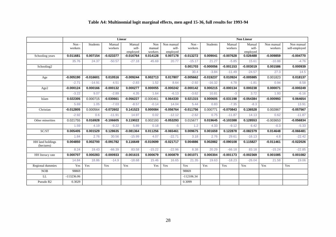
28
Table A4: Multinomial logit marginal effects, men aged 15-36, full results for 1993-94
Linear Non Linear
Non -
workers
Students Manual
workers
Manual
self-
employed
Non
manual
workers
Non manual
self-
employed
Non -
workers
Students Manual
workers
Manual
self-
employed
Non manual
workers
Non manual
self-employed
Schooling years 0.011681 0.007154 -0.023377 -0.016764 0.014128 0.007178 -0.013272 0.009041 -0.007628 0.026488 -0.009859 -0.004770
35.76 24.37 -50.57 -27.18 45.69 20.77 -15.17 21.27 -5.85 15.61 -10.88 -4.76
Schooling2 0.001703 -0.000056 -0.001153 -0.003019 0.001586 0.000939
30.4 -3.84 -11.49 -24.57 27.3 14.5
Age -0.005190 -0.016601 0.010516 -0.009244 0.002713 0.017807 -0.005662 -0.019237 0.010924 -0.005985 0.001823 0.018137
-2.71 -14.91 4.51 -2.83 1.52 8.64 -2.92 -16.32 4.78 -1.81 0.94 8.58
Age2 -0.000124 0.000166 -0.000132 0.000277 0.000055 -0.000242 -0.000142 0.000215 -0.000134 0.000238 0.000071 -0.000249
-3.22 9.07 -2.89 4.35 1.64 -6.13 -3.62 10.81 -3 3.72 1.93 -6.16
Islam 0.022305 0.000715 -0.030661 -0.056227 -0.000461 0.064330 0.021315 0.000605 -0.031198 -0.054384 -0.000993 0.064654
5.69 1.05 -7.03 -8.57 -0.14 14.04 5.44 0.83 -7.35 -8.3 . 13.91
Christian -0.012805 0.000564 -0.072602 0.141523 0.000084 -0.056764 -0.011756 0.000771 -0.070843 0.136528 0.002867 -0.057567
-2.92 0.6 -11.91 14.97 0.02 -12.12 -2.62 0.75 -11.87 14.13 0.62 -11.87
Other minorities 0.021755 0.016928 -0.106605 0.119022 0.002193 -0.053293 0.015677 0.019645 -0.103388 0.128553 -0.003653 -0.056834
1.59 4.19 -9.22 5.89 0.18 -5 1.2 4.33 -9.12 6.42 -0.3 -5.33
SC/ST 0.005405 0.001529 0.128635 -0.081364 0.011256 -0.065461 0.009675 0.001659 0.122878 -0.082379 0.014648 -0.066481
1.84 2.76 30.56 -15.99 4.07 -22.71 3.18 2.76 29.61 -16.13 4.8 -22.42
HH land holdings (hectares)
0.004850 0.002700 -0.091782 0.116649 -0.010699 -0.021717 0.004886 0.002882 -0.090108 0.115827 -0.011461 -0.022026
8.24 19.43 -66.39 83.58 -15.22 -22.96 8.38 20.29 -66.18 83.18 -15.24 -22.85
HH literacy rate 0.000707 0.000283 -0.000933 -0.001615 0.000679 0.000879 0.001071 0.000304 -0.001173 -0.002369 0.001085 0.001082
14.84 18.86 -14.9 -18.68 15.46 16.65 21.35 19.63 -18.23 -26.04 21.58 19.06
Regional dummies Yes Yes Yes Yes Yes Yes Yes Yes Yes Yes Yes Yes
NOB 98869 98869
LL -113236.06 -112106.34
Pseudo R2 0.3029 0.3099
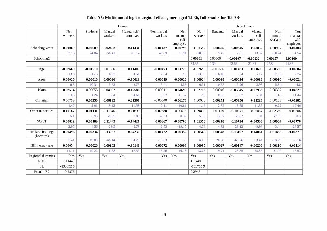
29
Table A5: Multinomial logit marginal effects, men aged 15-36, full results for 1999-00
Linear Non Linear
Non -
workers
Students Manual
workers
Manual self-
employed
Non manual
workers
Non
manual
self-
employed
Non -
workers
Students Manual
workers
Manual
self-
employed
Non
manual
workers
Non
manual
self-
employed
Schooling years 0.01069 0.00609 -0.02482 -0.01430 0.01437 0.00798 -0.01592 0.00665 0.00345 0.02052 -0.00987 -0.00483
32.16 24.04 -56.41 -26.14 46.69 21.91 -18.33 19.47 2.81 13.57 -10.74 -4.54
Schooling2 0.00181 0.00000 -0.00207 -0.00232 0.00157 0.00100
33.35 0.39 -22.66 -21.85 27.8 14.86
Age -0.02660 -0.01510 0.01506 0.01407 -0.00473 0.01729 -0.02696 -0.01636 0.01483 0.01605 -0.00560 0.01804
-13.8 -15.6 6.32 4.56 -2.54 7.6 -13.98 -16.16 6.4 5.17 -2.83 7.74
Age2 0.00026 0.00016 -0.00026 -0.00016 0.00019 -0.00020 0.00024 0.00018 -0.00024 -0.00018 0.00020 -0.00021
6.8 10.34 -5.52 -2.73 5.41 -4.53 6.31 10.95 -5.26 -2.93 5.34 -4.8
Islam 0.02514 0.00058 -0.04902 -0.02581 0.00211 0.04699 0.02713 0.00046 -0.05045 -0.02938 0.00397 0.04827
7.03 1.24 -12.4 -4.66 0.67 11.37 7.5 0.93 -13.27 -5.31 1.18 11.44
Christian 0.00799 0.00250 -0.06192 0.11369 -0.00048 -0.06178 0.00630 0.00271 -0.05956 0.11228 0.00109 -0.06282
1.47 2.91 -9.12 11.59 -0.11 -10.61 1.18 2.95 -8.98 11.35 0.22 -10.46
Other minorities 0.10187 0.01131 -0.11346 0.01699 -0.02288 0.00616 0.09436 0.01169 -0.10671 0.02087 -0.02529 0.00508
6.1 3.93 -9.05 0.83 -2.53 0.37 5.79 3.87 -8.62 1.01 -2.63 0.3
SC/ST 0.00822 0.00189 0.11445 -0.04420 0.00667 -0.08703 0.01353 0.00218 0.10724 -0.04500 0.00984 -0.08778
2.95 4.56 29.5 -9.79 2.53 -29.15 4.73 4.92 28.13 -9.93 3.44 -28.57
HH land holdings
(hectares) 0.00496 0.00334 -0.13287 0.14231 -0.01422 -0.00352 0.00540 0.00348 -0.13107 0.14061 -0.01465 -0.00377
5.41 19.89 -68.14 84.23 -13.53 -3 6.06 20.38 -68.76 83.41 -13.29 -3.16
HH literacy rate 0.00054 0.00026 -0.00105 -0.00140 0.00072 0.00093 0.00095 0.00027 -0.00147 -0.00200 0.00110 0.00114
11.11 19.22 -16.88 -17.53 15.26 16.13 18.75 19.71 -23.35 -23.86 21.09 18.53
Regional dummies Yes Yes Yes Yes Yes Yes Yes Yes Yes Yes Yes Yes
NOB 111449 111449
LL -133052.5 -131755.9
Pseudo R2 0.2876 0.2945
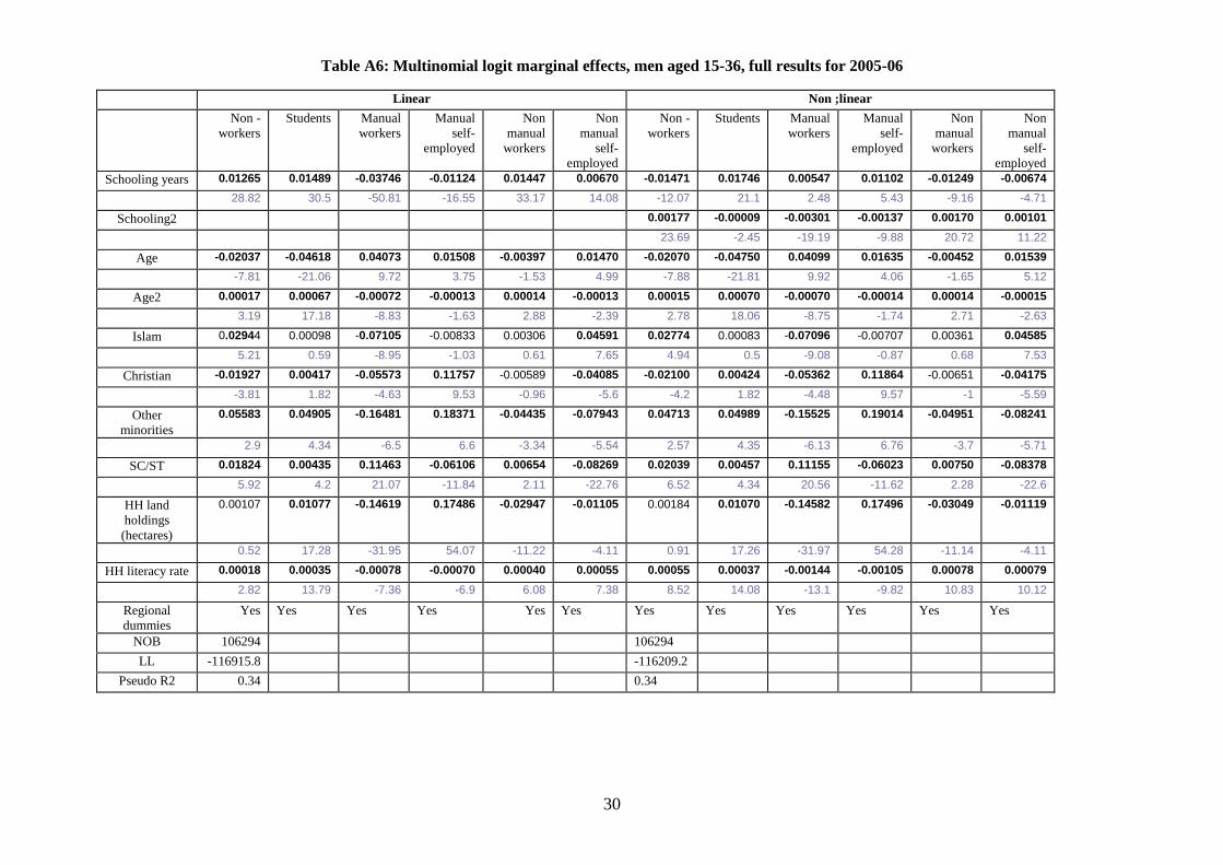
30
Table A6: Multinomial logit marginal effects, men aged 15-36, full results for 2005-06
Linear Non ;linear
Non -
workers
Students Manual
workers
Manual
self-
employed
Non
manual
workers
Non
manual
self-
employed
Non -
workers
Students Manual
workers
Manual
self-
employed
Non
manual
workers
Non
manual
self-
employed
Schooling years 0.01265 0.01489 -0.03746 -0.01124 0.01447 0.00670 -0.01471 0.01746 0.00547 0.01102 -0.01249 -0.00674
28.82 30.5 -50.81 -16.55 33.17 14.08 -12.07 21.1 2.48 5.43 -9.16 -4.71
Schooling2 0.00177 -0.00009 -0.00301 -0.00137 0.00170 0.00101
23.69 -2.45 -19.19 -9.88 20.72 11.22
Age -0.02037 -0.04618 0.04073 0.01508 -0.00397 0.01470 -0.02070 -0.04750 0.04099 0.01635 -0.00452 0.01539
-7.81 -21.06 9.72 3.75 -1.53 4.99 -7.88 -21.81 9.92 4.06 -1.65 5.12
Age2 0.00017 0.00067 -0.00072 -0.00013 0.00014 -0.00013 0.00015 0.00070 -0.00070 -0.00014 0.00014 -0.00015
3.19 17.18 -8.83 -1.63 2.88 -2.39 2.78 18.06 -8.75 -1.74 2.71 -2.63
Islam 0.02944 0.00098 -0.07105 -0.00833 0.00306 0.04591 0.02774 0.00083 -0.07096 -0.00707 0.00361 0.04585
5.21 0.59 -8.95 -1.03 0.61 7.65 4.94 0.5 -9.08 -0.87 0.68 7.53
Christian -0.01927 0.00417 -0.05573 0.11757 -0.00589 -0.04085 -0.02100 0.00424 -0.05362 0.11864 -0.00651 -0.04175
-3.81 1.82 -4.63 9.53 -0.96 -5.6 -4.2 1.82 -4.48 9.57 -1 -5.59
Other
minorities
0.05583 0.04905 -0.16481 0.18371 -0.04435 -0.07943 0.04713 0.04989 -0.15525 0.19014 -0.04951 -0.08241
2.9 4.34 -6.5 6.6 -3.34 -5.54 2.57 4.35 -6.13 6.76 -3.7 -5.71
SC/ST 0.01824 0.00435 0.11463 -0.06106 0.00654 -0.08269 0.02039 0.00457 0.11155 -0.06023 0.00750 -0.08378
5.92 4.2 21.07 -11.84 2.11 -22.76 6.52 4.34 20.56 -11.62 2.28 -22.6
HH land
holdings
(hectares)
0.00107 0.01077 -0.14619 0.17486 -0.02947 -0.01105 0.00184 0.01070 -0.14582 0.17496 -0.03049 -0.01119
0.52 17.28 -31.95 54.07 -11.22 -4.11 0.91 17.26 -31.97 54.28 -11.14 -4.11
HH literacy rate 0.00018 0.00035 -0.00078 -0.00070 0.00040 0.00055 0.00055 0.00037 -0.00144 -0.00105 0.00078 0.00079
2.82 13.79 -7.36 -6.9 6.08 7.38 8.52 14.08 -13.1 -9.82 10.83 10.12
Regional
dummies
Yes Yes Yes Yes Yes Yes Yes Yes Yes Yes Yes Yes
NOB 106294 106294
LL -116915.8 -116209.2
Pseudo R2 0.34 0.34

31
Table A7: Multinomial logit marginal effects, women aged 15-36, full results for 1993-94
Linear Non linear
Non -
workers
Students Manual
workers
Manual
self-
employed
Non
manual
workers
Non
manual
self-
employed
Non -
workers
Students Manual
workers
Manual
self-
employed
Non
manual
workers
Non
manual
self-
employed
Schooling
years 0.013463 0.000907 -0.005358 -0.012985 0.003782 0.000192 0.003453 0.001220 -0.001570 0.000423 -0.002033 -0.001492
31.87 15 -31.07 -35.64 29.7 2.09 2.79 15.12 -3.17 0.38 -6.46 -5.84
Schooling2 0.001088 -0.000020 -0.000358 -0.001225 0.000386 0.000129
10.14 -8.63 -7.75 -12.49 17.74 7.25
Age 0.022762 -0.002584 -0.004743 -0.013569 -0.001141 -0.000725 0.022345 -0.002563 -0.004274 -0.012149 -0.002503 -0.000856
11.39 -10.75 -7.45 -7.91 -1.88 -1.36 11.44 -11.59 -7.21 -7.41 -3.53 -1.59
Age2 -0.000481 0.000031 0.000102 0.000281 0.000041 0.000027 -0.000478 0.000033 0.000093 0.000259 0.000065 0.000028
-12.3 7.88 8.11 8.33 3.55 2.58 -12.52 9 7.99 8.03 4.86 2.7
Islam 0.108108 -0.000431 -0.024966 -0.074537 -0.004197 -0.003976 0.103479 -0.000444 -0.023406 -0.072036 -0.003803 -0.003790
35.33 -4.32 -26.34 -28.1 -4 -4.78 34.21 -4.66 -25.36 -28.47 -3.03 -4.46
Christian -0.192242 0.000526 -0.002595 0.178446 0.007243 0.008621 -0.188122 0.000518 -0.002385 0.168949 0.011488 0.009552
-21.01 3.1 -1.22 19.95 4.6 4.65 -20.93 3.17 -1.2 19.32 5.64 4.94
Other
minorities -0.316061 0.002077 -0.010587 0.327842 -0.001522 -0.001750 -0.313116 0.002411 -0.009420 0.325303 -0.003304 -0.001874
-15.79 2.96 -2.57 16.55 -0.35 -0.5 -15.65 3.18 -2.42 16.48 -0.75 -0.54
SC/ST -0.056381 -0.000254 0.032142 0.016382 0.005256 0.002855 -0.054072 -0.000269 0.029804 0.015190 0.006299 0.003048
-16.41 -2.73 21.49 5.77 4.82 3.16 -16.01 -3 20.64 5.58 5 3.33
HH land
holdings
(hectares)
0.012911 0.000047 -0.016694 0.010995 -0.002796 -0.004463 0.012385 0.000037 -0.015501 0.010342 -0.002844 -0.004420
21.52 4.19 -37.81 36.36 -10.46 -14.54 20 3.49 -33.96 35.03 -9.54 -14.32
HH literacy
rate 0.001009 0.000058 -0.000486 -0.000558 -0.000005 -0.000018 0.001036 0.000054 -0.000496 -0.000738 0.000129 0.000016
18.41 13.33 -24.01 -11.9 -0.31 -1.3 18.48 13.73 -24.94 -15.74 6.53 1.14
Regional
dummies
Yes Yes Yes Yes Yes Yes Yes Yes Yes Yes Yes Yes
NOB 94260 94260
LL -76853.708 -76434.04
Pseudo R2 0.3102 0.3139
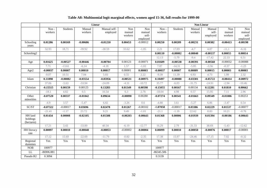
32
Table A8: Multinomial logit marginal effects, women aged 15-36, full results for 1999-00
Linear Non Linear
Non -
workers
Students Manual
workers
Manual self-
employed
Non
manual
workers
Non
manual
self-
employed
Non -
workers
Students Manual
workers
Manual
self-
employed
Non
manual
workers
Non
manual
self-
employed
Schooling
years 0.01286 0.00169 -0.00686 -0.01210 0.00453 -0.00012 0.00250 0.00209 -0.00231 0.00382 -0.00413 -0.00198
32.93 18.71 -39.92 -38.59 33.62 -1.05 2.21 17.69 -4.7 4.07 -11.1 -6.16
Schooling2 0.00110 -0.00002 -0.00040 -0.00137 0.00055 0.00014
12.13 -5.79 -9.4 -17.42 22.33 6.51
Age 0.01625 -0.00527 -0.00446 -0.00704 0.00123 -0.00071 0.01609 -0.00538 -0.00391 -0.00560 -0.00032 -0.00088
7.71 -13.61 -6.14 -4.18 1.57 -1.02 7.87 -14.31 -5.85 -3.56 -0.37 -1.23
Age2 -0.00037 0.00007 0.00010 0.00017 0.00001 0.00003 -0.00037 0.00007 0.00009 0.00015 0.00003 0.00003
-9.07 10.51 7.04 5.03 0.55 2.22 -9.39 11.39 6.93 4.73 1.99 2.32
Islam 0.11098 -0.00082 -0.03554 -0.05956 -0.00531 -0.00975 0.10497 -0.00088 -0.03301 -0.05722 -0.00414 -0.00972
37.06 -5.63 -33.94 -24.09 -4.31 -10.72 35.77 -6.03 -31.75 -24.91 -2.94 -10.46
Christian -0.15515 0.00159 0.00125 0.13283 0.01349 0.00598 -0.15055 0.00167 0.00134 0.12281 0.01810 0.00662
-18.1 4.82 0.5 16.54 6.3 2.76 -18.04 4.98 0.57 15.95 7.11 2.96
Other
minorities -0.07520 0.00337 -0.01842 0.09634 -0.00890 0.00280 -0.07274 0.00341 -0.01663 0.09349 -0.01006 0.00253
-4.9 3.57 -5.47 6.82 -3.26 0.6 -4.88 3.61 -5.27 6.86 -3.47 0.54
SC/ST -0.07322 -0.00017 0.03696 0.02478 0.01267 -0.00102 -0.07058 -0.00017 0.03386 0.02229 0.01537 -0.00077
-21.41 -1.17 23.72 9.21 9.49 -1.01 -21.1 -1.19 22.62 8.83 10.21 -0.76
HH land
holdings
(hectares)
0.01434 0.00008 -0.02105 0.01508 -0.00203 -0.00643 0.01368 0.00006 -0.01939 0.01394 -0.00186 -0.00643
17.21 3.43 -33.89 40.34 -6.19 -12.77 16.29 2.79 -31.33 38.69 -5.43 -12.62
HH literacy
rate 0.00097 0.00010 -0.00048 -0.00053 -0.00002 -0.00004 0.00099 0.00010 -0.00050 -0.00076 0.00017 -0.00001
17.12 15.69 -22.69 -11.79 -0.82 -2.35 17.38 15.97 -24.46 -17.15 7.02 -0.32
Regional
dummies
Yes Yes Yes Yes Yes Yes Yes Yes Yes Yes Yes Yes
NOB 100977 100977
LL -86906.881 -86345.506
Pseudo R2 0.3094 0.3139
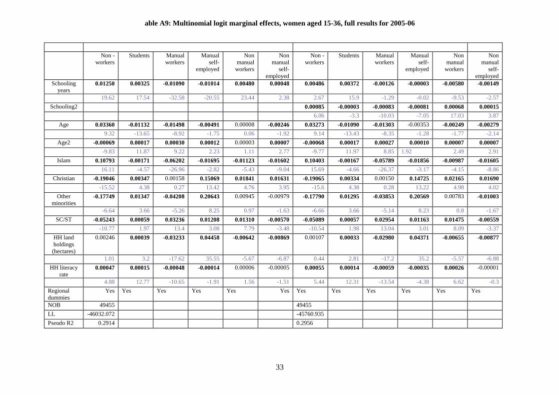
33
able A9: Multinomial logit marginal effects, women aged 15-36, full results for 2005-06
Non -
workers
Students Manual
workers
Manual
self-
employed
Non
manual
workers
Non
manual
self-
employed
Non -
workers
Students Manual
workers
Manual
self-
employed
Non
manual
workers
Non
manual
self-
employed
Schooling
years 0.01250 0.00325 -0.01090 -0.01014 0.00480 0.00048 0.00486 0.00372 -0.00126 -0.00003 -0.00580 -0.00149
19.62 17.54 -32.58 -20.55 23.44 2.38 2.67 15.9 -1.29 -0.02 -9.53 -2.57
Schooling2 0.00085 -0.00003 -0.00083 -0.00081 0.00068 0.00015
6.06 -3.3 -10.03 -7.05 17.03 3.87
Age 0.03360 -0.01132 -0.01498 -0.00491 0.00008 -0.00246 0.03273 -0.01090 -0.01303 -0.00353 -0.00249 -0.00279
9.32 -13.65 -8.92 -1.75 0.06 -1.92 9.14 -13.43 -8.35 -1.28 -1.77 -2.14
Age2 -0.00069 0.00017 0.00030 0.00012 0.00003 0.00007 -0.00068 0.00017 0.00027 0.00010 0.00007 0.00007
-9.83 11.87 9.22 2.23 1.11 2.77 -9.77 11.97 8.85 1.92 2.49 2.91
Islam 0.10793 -0.00171 -0.06202 -0.01695 -0.01123 -0.01602 0.10403 -0.00167 -0.05789 -0.01856 -0.00987 -0.01605
16.11 -4.57 -26.96 -2.82 -5.43 -9.04 15.69 -4.66 -26.37 -3.17 -4.15 -8.86
Christian -0.19046 0.00347 0.00158 0.15069 0.01841 0.01631 -0.19065 0.00334 0.00150 0.14725 0.02165 0.01690
-15.52 4.38 0.27 13.42 4.76 3.95 -15.6 4.38 0.28 13.22 4.98 4.02
Other
minorities -0.17749 0.01347 -0.04208 0.20643 0.00945 -0.00979 -0.17790 0.01295 -0.03853 0.20569 0.00783 -0.01003
-6.64 3.66 -5.26 8.25 0.97 -1.63 -6.66 3.66 -5.14 8.23 0.8 -1.67
SC/ST -0.05243 0.00059 0.03236 0.01208 0.01310 -0.00570 -0.05089 0.00057 0.02954 0.01163 0.01475 -0.00559
-10.77 1.97 13.4 3.08 7.79 -3.48 -10.54 1.98 13.04 3.01 8.09 -3.37
HH land
holdings
(hectares)
0.00246 0.00039 -0.03233 0.04458 -0.00642 -0.00869 0.00107 0.00033 -0.02980 0.04371 -0.00655 -0.00877
1.01 3.2 -17.62 35.55 -5.67 -6.87 0.44 2.81 -17.2 35.2 -5.57 -6.88
HH literacy
rate 0.00047 0.00015 -0.00048 -0.00014 0.00006 -0.00005 0.00055 0.00014 -0.00059 -0.00035 0.00026 -0.00001
4.88 12.77 -10.65 -1.91 1.56 -1.51 5.44 12.31 -13.54 -4.38 6.62 -0.3
Regional
dummies
Yes Yes Yes Yes Yes Yes Yes Yes Yes Yes Yes Yes
NOB 49455 49455
LL -46032.072 -45760.935
Pseudo R2 0.2914 0.2956
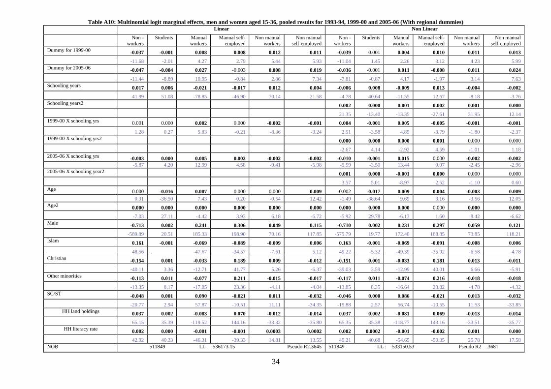
34
Table A10: Multinomial logit marginal effects, men and women aged 15-36, pooled results for 1993-94, 1999-00 and 2005-06 (With regional dummies) Linear Non Linear
Non -
workers
Students Manual
workers
Manual self-
employed
Non manual
workers
Non manual
self-employed
Non -
workers
Students Manual
workers
Manual self-
employed
Non manual
workers
Non manual
self-employed
Dummy for 1999-00 -0.037 -0.001 0.008 0.008 0.012 0.011 -0.039 0.001 0.004 0.010 0.011 0.013
-11.68 -2.01 4.27 2.79 5.44 5.93 -11.04 1.45 2.26 3.12 4.23 5.99
Dummy for 2005-06 -0.047 -0.004 0.027 -0.003 0.008 0.019 -0.036 -0.001 0.011 -0.008 0.011 0.024
-11.44 -8.89 10.95 -0.84 2.86 7.34 -7.81 -0.87 4.17 -1.97 3.14 7.63
Schooling years 0.017 0.006 -0.021 -0.017 0.012 0.004 -0.006 0.008 -0.009 0.013 -0.004 -0.002
41.99 51.08 -78.85 -46.90 70.14 21.58 -4.78 40.64 -11.55 12.67 -8.18 -3.76
Schooling years2 0.002 0.000 -0.001 -0.002 0.001 0.000
21.35 -13.40 -13.35 -27.61 31.95 12.14
1999-00 X schooling yrs 0.001 0.000 0.002 0.000 -0.002 -0.001 0.004 -0.001 0.005 -0.005 -0.001 -0.001
1.28 0.27 5.83 -0.21 -8.36 -3.24 2.51 -3.58 4.89 -3.79 -1.80 -2.37
1999-00 X schooling yrs2 0.000 0.000 0.000 0.001 0.000 0.000
-2.67 4.14 -2.92 4.59 -1.01 1.18
2005-06 X schooling yrs -0.003 0.000 0.005 0.002 -0.002 -0.002 -0.010 -0.001 0.015 0.000 -0.002 -0.002
-5.87 4.20 12.99 4.58 -9.41 -5.98 -5.59 -3.50 13.44 0.07 -2.45 -2.96
2005-06 X schooling year2 0.001 0.000 -0.001 0.000 0.000 0.000
3.57 5.01 -8.97 2.52 -1.10 0.60
Age 0.000 -0.016 0.007 0.000 0.000 0.009 -0.002 -0.017 0.009 0.004 -0.003 0.009
0.31 -36.50 7.43 0.20 -0.54 12.42 -1.49 -38.64 9.69 3.16 -3.56 12.05
Age2 0.000 0.000 0.000 0.000 0.000 0.000 0.000 0.000 0.000 0.000 0.000 0.000
-7.03 27.11 -4.42 3.93 6.18 -6.72 -5.92 29.78 -6.13 1.60 8.42 -6.62
Male -0.713 0.002 0.241 0.306 0.049 0.115 -0.710 0.002 0.231 0.297 0.059 0.121
-589.89 20.51 185.33 198.90 70.16 117.85 -575.79 19.77 172.40 188.85 73.85 118.21
Islam 0.161 -0.001 -0.069 -0.089 -0.009 0.006 0.163 -0.001 -0.069 -0.091 -0.008 0.006
48.56 . -47.67 -34.57 -7.61 5.12 49.22 -5.32 -49.39 -35.92 -6.58 4.78
Christian -0.154 0.001 -0.033 0.189 0.009 -0.012 -0.151 0.001 -0.033 0.181 0.013 -0.011
-40.11 3.36 -12.71 41.77 5.26 -6.37 -39.03 3.59 -12.99 40.01 6.66 -5.91
Other minorities -0.113 0.011 -0.077 0.211 -0.015 -0.017 -0.117 0.011 -0.074 0.216 -0.018 -0.018
-13.35 8.17 -17.05 23.36 -4.11 -4.04 -13.85 8.35 -16.64 23.82 -4.78 -4.32
SC/ST -0.048 0.001 0.090 -0.021 0.011 -0.032 -0.046 0.000 0.086 -0.021 0.013 -0.032
-20.77 2.94 57.87 -10.51 11.11 -34.35 -19.88 2.57 56.74 -10.55 11.53 -33.85
HH land holdings 0.037 0.002 -0.083 0.070 -0.012 -0.014 0.037 0.002 -0.081 0.069 -0.013 -0.014
65.15 35.39 -119.52 144.16 -33.32 -35.80 65.35 35.38 -118.77 143.16 -33.51 -35.77
HH literacy rate 0.002 0.000 -0.001 -0.001 0.0003 0.0002 0.002 0.0002 -0.001 -0.002 0.001 0.000
42.92 40.33 -46.31 -39.33 14.81 13.55 49.21 40.68 -54.65 -50.35 25.78 17.58
NOB 511849 LL -536173.15 Pseudo R2.3645 511849 LL : -533150.53 Pseudo R2 .3681
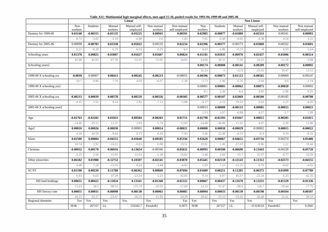
35
Table A11: Multinomial logit marginal effects, men aged 15-36, pooled results for 1993-94, 1999-00 and 2005-06
Linear Non Linear
Non -workers
Students Manual workers
Manual self-employed
Non manual workers
Non manual self-employed
Non -workers
Students Manual workers
Manual self-employed
Non manual workers
Non manual self-employed
Dummy for 1999-00 0.03140 -0.00315 -0.01135 -0.03225 0.00945 0.00591 0.02985 -0.00077 -0.01809 -0.02333 0.00241 0.00993
8.72 -3.82 -3.19 -6.98 2.6 1.63 7.61 -0.48 -4.65 -4.38 0.54 2.22
Dummy for 2005-06 0.00098 -0.00783 0.03338 -0.05022 0.00135 0.02234 0.02396 -0.00377 -0.00173 -0.05869 0.00332 0.03691
0.21 -9.18 6.79 -8.19 0.29 4.4 4.03 -1.86 -0.33 -8 0.55 5.64
Schooling years 0.01378 0.00825 -0.03007 -0.01627 0.01607 0.00824 -0.01181 0.01035 -0.00970 0.02437 -0.01006 -0.00314
45.68 42.93 -67.39 -32.01 55.95 24.85 -14.06 30.31 -7.36 16.23 -11.16 -3.08
Schooling years2 0.00174 -0.00008 -0.00141 -0.00289 0.00172 0.00092
32.23 -5 -12.9 -25.02 30.47 13.53
1999-00 X schooling yrs -0.0039 0.00007 0.00411 0.00245 -0.00213 -0.00055 -0.00396 -0.00073 0.01112 -0.00565 0.00069 -0.00147
-10.7 0.86 7.76 4.03 -6.07 -1.38 -3.73 -1.96 6.76 -2.94 0.6 -1.14
1999-00 X schooling yrs2 0.00001 0.00005 -0.00062 0.00075 -0.00020 0.00002
0.1 2.36 -4.4 4.92 -2.86 0.25
2005-06 X schooling yrs -0.00215 0.00039 0.00578 0.00229 -0.00326 -0.00305 -0.00577 -0.00107 0.02069 -0.00500 -0.00185 -0.00700
-4.41 3.52 9.14 2.92 -7.12 -5.88 -4.17 -2.15 10.52 -2.03 -1.25 -4.29
2005-06 X schooling year2 0.00013 0.00008 -0.00113 0.00085 -0.00015 0.00021
1.53 3.07 -6.98 4.57 -1.7 1.99
Age -0.01763 -0.02202 0.01833 0.00584 -0.00203 0.01751 -0.01798 -0.02393 0.01847 0.00815 -0.00285 0.01815
-14.46 -29.12 11.57 2.93 -1.74 12.69 -14.68 -30.86 11.92 4.07 -2.28 12.86
Age2 0.00010 0.00026 -0.00030 0.00001 0.00014 -0.00021 0.00008 0.00030 -0.00029 -0.00002 0.00015 -0.00022
4.18 20.59 -9.64 0.15 6.18 -7.95 3.36 22.48 -9.53 -0.4 6.19 -8.31
Islam 0.02590 0.00084 -0.04555 -0.03640 0.00185 0.05336 0.02620 0.00067 -0.04651 -0.03716 0.00274 0.05406
10.74 1.92 -16.21 -9.65 0.88 19.51 10.81 1.46 -17.07 -9.86 1.21 19.44
Christian -0.00932 0.00170 -0.06916 0.13654 -0.00346 -0.05631 -0.00993 0.00188 -0.06690 0.13443 -0.00228 -0.05720
-3.25 2.56 -15.91 22.63 -1.28 -16.82 -3.48 2.66 -15.7 22.07 -0.77 -16.59
Other minorities 0.06182 0.01988 -0.12752 0.10597 -0.02145 -0.03870 0.05441 0.02118 -0.12143 0.11312 -0.02573 -0.04155
6.48 7.18 -15.91 8.24 -3.48 -4.63 5.93 7.23 -15.35 8.79 -4.02 -4.93
SC/ST 0.01190 0.00230 0.11788 -0.06362 0.00849 -0.07694 0.01609 0.00251 0.11205 -0.06375 0.01099 -0.07789
6.93 6.65 47.28 -22.24 5.23 -42.85 9.14 6.87 45.57 -22.24 6.25 -42.35
HH land holdings 0.00651 0.00422 -0.11834 0.13341 -0.01268 -0.01312 0.00667 0.00437 -0.11670 0.13231 -0.01329 -0.01336
12.63 34.5 -98.31 125.74 -20.55 -17.69 13.23 35.47 -98.6 126.7 -20.44 -17.75
HH literacy rate 0.00055 0.00031 -0.00098 -0.00138 0.00065 0.00085 0.00094 0.00033 -0.00139 -0.00198 0.00104 0.00107
18.15 32.27 -23.67 -26.55 21.95 24.29 29.62 33.12 -32.65 -36.48 31.61 28.53
Regional dummies Yes Yes Yes Yes Yes Yes Yes Yes Yes Yes Yes Yes
NOB 267157 LL -316342.7 PseudoR2 0.2875 NOB 267157 LL -313230.03 PseudoR2 0.2945
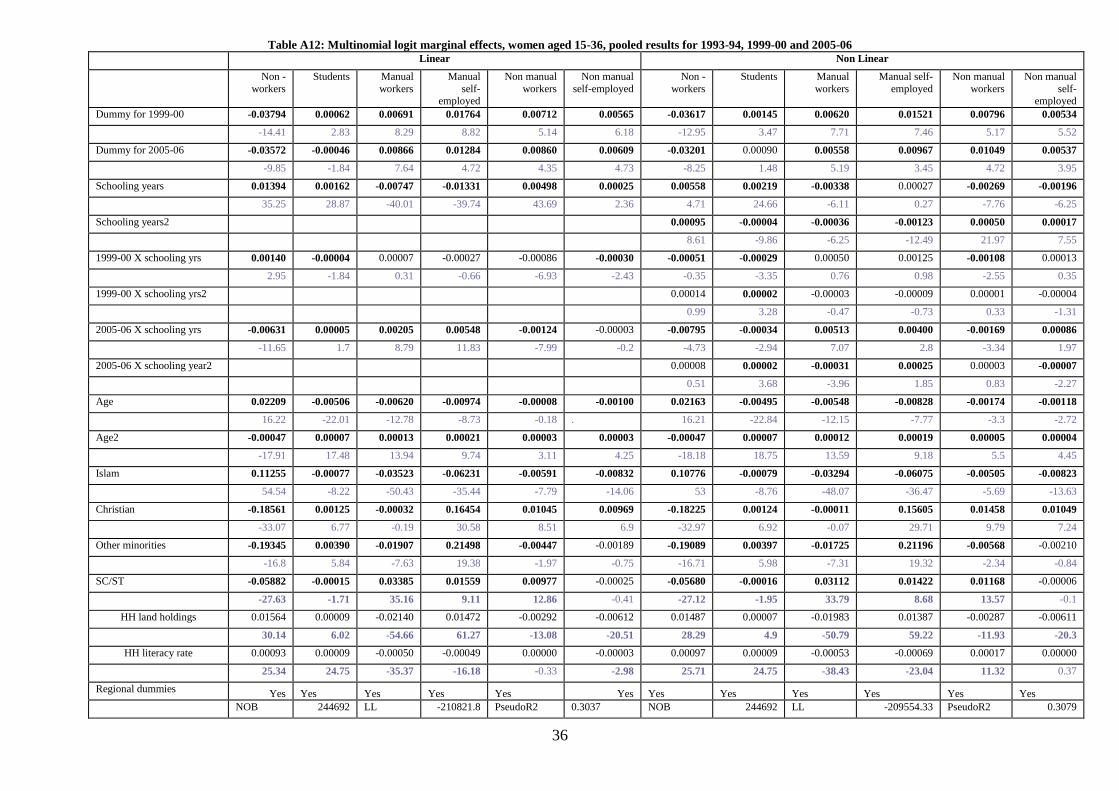
36
Table A12: Multinomial logit marginal effects, women aged 15-36, pooled results for 1993-94, 1999-00 and 2005-06 Linear Non Linear
Non -
workers
Students Manual
workers
Manual
self-employed
Non manual
workers
Non manual
self-employed
Non -
workers
Students Manual
workers
Manual self-
employed
Non manual
workers
Non manual
self-employed
Dummy for 1999-00 -0.03794 0.00062 0.00691 0.01764 0.00712 0.00565 -0.03617 0.00145 0.00620 0.01521 0.00796 0.00534
-14.41 2.83 8.29 8.82 5.14 6.18 -12.95 3.47 7.71 7.46 5.17 5.52
Dummy for 2005-06 -0.03572 -0.00046 0.00866 0.01284 0.00860 0.00609 -0.03201 0.00090 0.00558 0.00967 0.01049 0.00537
-9.85 -1.84 7.64 4.72 4.35 4.73 -8.25 1.48 5.19 3.45 4.72 3.95
Schooling years 0.01394 0.00162 -0.00747 -0.01331 0.00498 0.00025 0.00558 0.00219 -0.00338 0.00027 -0.00269 -0.00196
35.25 28.87 -40.01 -39.74 43.69 2.36 4.71 24.66 -6.11 0.27 -7.76 -6.25
Schooling years2 0.00095 -0.00004 -0.00036 -0.00123 0.00050 0.00017
8.61 -9.86 -6.25 -12.49 21.97 7.55
1999-00 X schooling yrs 0.00140 -0.00004 0.00007 -0.00027 -0.00086 -0.00030 -0.00051 -0.00029 0.00050 0.00125 -0.00108 0.00013
2.95 -1.84 0.31 -0.66 -6.93 -2.43 -0.35 -3.35 0.76 0.98 -2.55 0.35
1999-00 X schooling yrs2 0.00014 0.00002 -0.00003 -0.00009 0.00001 -0.00004
0.99 3.28 -0.47 -0.73 0.33 -1.31
2005-06 X schooling yrs -0.00631 0.00005 0.00205 0.00548 -0.00124 -0.00003 -0.00795 -0.00034 0.00513 0.00400 -0.00169 0.00086
-11.65 1.7 8.79 11.83 -7.99 -0.2 -4.73 -2.94 7.07 2.8 -3.34 1.97
2005-06 X schooling year2 0.00008 0.00002 -0.00031 0.00025 0.00003 -0.00007
0.51 3.68 -3.96 1.85 0.83 -2.27
Age 0.02209 -0.00506 -0.00620 -0.00974 -0.00008 -0.00100 0.02163 -0.00495 -0.00548 -0.00828 -0.00174 -0.00118
16.22 -22.01 -12.78 -8.73 -0.18 . 16.21 -22.84 -12.15 -7.77 -3.3 -2.72
Age2 -0.00047 0.00007 0.00013 0.00021 0.00003 0.00003 -0.00047 0.00007 0.00012 0.00019 0.00005 0.00004
-17.91 17.48 13.94 9.74 3.11 4.25 -18.18 18.75 13.59 9.18 5.5 4.45
Islam 0.11255 -0.00077 -0.03523 -0.06231 -0.00591 -0.00832 0.10776 -0.00079 -0.03294 -0.06075 -0.00505 -0.00823
54.54 -8.22 -50.43 -35.44 -7.79 -14.06 53 -8.76 -48.07 -36.47 -5.69 -13.63
Christian -0.18561 0.00125 -0.00032 0.16454 0.01045 0.00969 -0.18225 0.00124 -0.00011 0.15605 0.01458 0.01049
-33.07 6.77 -0.19 30.58 8.51 6.9 -32.97 6.92 -0.07 29.71 9.79 7.24
Other minorities -0.19345 0.00390 -0.01907 0.21498 -0.00447 -0.00189 -0.19089 0.00397 -0.01725 0.21196 -0.00568 -0.00210
-16.8 5.84 -7.63 19.38 -1.97 -0.75 -16.71 5.98 -7.31 19.32 -2.34 -0.84
SC/ST -0.05882 -0.00015 0.03385 0.01559 0.00977 -0.00025 -0.05680 -0.00016 0.03112 0.01422 0.01168 -0.00006
-27.63 -1.71 35.16 9.11 12.86 -0.41 -27.12 -1.95 33.79 8.68 13.57 -0.1
HH land holdings 0.01564 0.00009 -0.02140 0.01472 -0.00292 -0.00612 0.01487 0.00007 -0.01983 0.01387 -0.00287 -0.00611
30.14 6.02 -54.66 61.27 -13.08 -20.51 28.29 4.9 -50.79 59.22 -11.93 -20.3
HH literacy rate 0.00093 0.00009 -0.00050 -0.00049 0.00000 -0.00003 0.00097 0.00009 -0.00053 -0.00069 0.00017 0.00000
25.34 24.75 -35.37 -16.18 -0.33 -2.98 25.71 24.75 -38.43 -23.04 11.32 0.37
Regional dummies Yes Yes Yes Yes Yes Yes Yes Yes Yes Yes Yes Yes
NOB 244692 LL -210821.8 PseudoR2 0.3037 NOB 244692 LL -209554.33 PseudoR2 0.3079

37
Related Documents