Dynamic Natural Monopoly Regulation Time Inconsistency ...

Dynamic Natural Monopoly Regulation:Time Inconsistency, Asymmetric Information,

and Political Environments

Claire S.H. Lim∗

Cornell UniversityAli Yurukoglu†

Stanford University ‡

July 20, 2014

Abstract

This paper quantitatively assesses time inconsistency, asymmetric information, and polit-ical ideology in monopoly regulation of electricity distribution companies. Empirically, weestimate that (1) there is under-investment in electricity distribution capital to reduce poweroutages, (2) more conservative political environments have higher regulated returns, and (3)more conservative political environments have more electricity lost in distribution. We explainthese empirical results with an estimated dynamic game model of utility regulation featuringinvestment and asymmetric information. We quantify the value of regulatory commitment ininducing more investment. Conservative regulators improve welfare losses due to time incon-sistency, but worsen losses from asymmetric information.

Keywords: Regulation, Natural Monopoly, Electricity, Political Environment, Dynamic GameEstimationJEL Classification: D72, D78, L43, L94

1 Introduction

In macroeconomics, public finance, and industrial organization and regulation, policy makers suf-fer from the inability to credibly commit to future policies (Coase (1972), Kydland and Prescott(1977)) and from the existence of information that is privately known to the agents subject totheir policies (Mirrlees (1971), Baron and Myerson (1982)). These two obstacles, “time inconsis-tency” and “asymmetric information,” make it difficult, if not impossible, for regulation to achieve

∗Department of Economics, 404 Uris Hall, Ithaca, NY 14853 (e-mail: [email protected])†Graduate School of Business, 655 Knight Way, Stanford, CA 94305 (e-mail: Yurukoglu [email protected])‡We thank Jose Miguel Abito, John Asker, David Baron, Lanier Benkard, Patrick Bolton, Severin Borenstein,

Dan O’Neill, Ariel Pakes, Steven Puller, Nancy Rose, Stephen Ryan, Mario Samano, David Sappington, RichardSchmalensee, Frank Wolak, and participants at seminars and conferences at Columbia, Cornell, Harvard, MIT, Mon-treal, NBER, NYU Stern, Olin Business School, SUNY-Albany, UC Davis, and Wharton for their comments andsuggestions.

1

first-best policies. This paper analyzes these two forces and their interaction with the political en-vironment in the context of regulating the U.S. electricity distribution industry, a natural monopolysector with yearly revenues of $320 billion.

The time inconsistency problem in this context is the possibility of regulatory hold-up in rate-of-return regulation. The regulator would like to commit to a fair return on irreversible investmentsex ante. Once the investments are sunk, the regulator is tempted to adjudicate a lower returnthan promised (Baron and Besanko (1987), Gilbert and Newbery (1994), Lewis and Sappington(1991)).1 The utility realizes this dynamic, resulting in under-investment by the regulated utility.2

The asymmetric information problem in this context is moral hazard: the utility can take costlyactions that improve productivity, but the regulator can not directly measure the extent of theseactions (Baron and Myerson (1982), Laffont and Tirole (1993) and Armstrong and Sappington(2007)).3

These two forces interact with the political environment. A central theme of this paper is thatregulatory environments which place a higher weight on utility profits vis-a-vis consumer surplusgrant higher rates of return, which encourages more investment, alleviating inefficiencies due totime inconsistency and the fear of regulatory hold-up. However, these regulatory environments en-gage in less intense auditing of the utility’s unobserved effort choices, leading to more inefficiencyin production, exacerbating the problem of asymmetric information.

The core empirical evidence supporting this formulation is twofold. First, we estimate that thereis under-investment in electricity distribution capital in the U.S. To do so, we estimate the costsof improving reliability by capital investment. We combine those estimates with surveyed valuesof reliability. At current mean capital levels, the benefit of investment in reducing power outagesexceeds the costs. Second, regulated rates of return are higher, but measures of productivity arelower with more conservative regulatory environments. We measure the ideology of the regulatoryenvironment using both cross-sectional variation in how a state’s U.S. Congressmen vote, andwithin-state time variation in the party affiliation of state regulatory commissioners. Both resultshold using either source of variation.

We explain these core empirical findings with a dynamic game theoretic model of the regulator-utility interaction. The utility invests in capital, and exerts effort that affects productivity to maxi-mize its firm value. The regulator chooses a return on the utility’s capital and a degree of auditingof the utility’s effort choice to maximize a weighted average of utility profits and consumer sur-plus. The regulator can not commit to future policies, but has a costly auditing technology. We use

1See also Section 3.4.1 of Armstrong and Sappington (2007) for more references and discussion of limited com-mitment, regulation, and expropriation of sunk investments.

2In our context, under-investment manifests itself as an aging infrastructure prone to too many power outages.3Adverse selection is also at play in the literature on natural monopoly regulation. This paper focuses on moral

hazard.

2

the solution concept of Markov Perfect Equilibrium. Markov perfection in the equilibrium notionimplies a time-inconsistency problem for the regulator which in turn implies socially sub-optimalinvestment levels by the utility.

We estimate the model’s parameters using a two-step estimation procedure following Bajari etal. (2007) and Pakes et al. (2007). Given the core empirical results and the model’s comparativestatics, we estimate that more conservative political environments place relatively more weight onutility profits than less conservative political environments. More weight on utility profits can begood for social welfare because it leads to stronger investment incentives, which in turn mitigatesthe time inconsistency problem. However, this effect must be traded-off with the tendency for laxauditing which reduces managerial effort, productivity, and social welfare.

We use the estimated parameters to simulate appropriate rules and design of institutions toincrease investment incentives and balance the tension between investment incentives and effortprovision. We counterfactually simulate outcomes when (1) the regulator can commit to futurerates of return, (2) there are minimum auditing requirements for the regulator, and (3) the regula-tory board must maintain a minimum level of minority representation. In the first counterfactualwith commitment, we find that regulators would like to substantially increase rates of return toprovide incentives for capital investment. This result is consistent with recent efforts by somestate legislatures to bypass the traditional regulatory process and legislate more investment in elec-tricity distribution capital. This result also implies that tilting the regulatory commission towardsconservatives, analogous to the idea in Rogoff (1985) for central bankers, can mitigate the timeinconsistency problem. However, such a policy would be enhanced by minimum auditing require-ments. Minority representation requirements reduce uncertainty for the utility and variance ininvestment rates, but have quantitatively weak effects on investment and productivity levels.

This paper contributes to literatures in both industrial organization and political economy. Withinindustrial organization and regulation, the closest papers are Timmins (2002), Wolak (1994), Gag-nepain and Ivaldi (2002), and Abito (2013). Timmins (2002) estimates regulator preferences ina dynamic model of a municipal water utility. In that setting, the regulator controls the utilitydirectly which led to a theoretical formulation of a single-agent decision problem. By contrast,this paper studies a dynamic game where there is a strategic interaction between the regulator andutility. Wolak (1994) pioneered the empirical study of the regulator-utility strategic interactionin static settings with asymmetric information. More recently, Gagnepain and Ivaldi (2002) andAbito (2013) use static models of regulator-utility asymmetric information to study transportationservice and environmental regulation of power generation, respectively. This paper adds an in-vestment problem in parallel to the asymmetric information. Adding investment brings issues ofcommitment and dynamic decisions in regulation into focus. Lyon and Mayo (2005) study the

3

possibility of regulatory hold-up in power generation.4 Levy and Spiller (1994) present a series ofcase studies on regulation of telecommunications firms, mostly in developing countries. They con-clude that “without... commitment long-term investment will not take place, [and] that achievingsuch commitment may require inflexible regulatory regimes.” Our paper is also related to staticproduction function estimates for electricity distribution such as Growitsch et al. (2009) and Nille-sen and Pollitt (2011). On the political economy side, the most closely related papers are Besleyand Coate (2003) and Leaver (2009). Besley and Coate (2003) compare electricity pricing underappointed and elected regulators. Leaver (2009) analyzes how regulators’ desire to avoid publiccriticisms lead them to behave inefficiently in rate reviews.

More broadly, economic regulation is an important feature of banking, health insurance, water,waste management, and natural gas delivery. Regulators in these sectors are appointed by electedofficials or elected themselves, whether they be a member of the Federal Reserve Board5, a stateinsurance commissioner, or a state public utility commissioner. Therefore, different political envi-ronments can give rise to regulators that make systematically different decisions which ultimatelydetermine industry outcomes as we find in electric power distribution.

Finally, our analysis has two implications for environmental policy. First, investments in elec-tricity distribution are necessary to accommodate new technologies such as smart meters and dis-tributed generation. Our findings quantify a fundamental obstacle to incentivizing investmentwhich is the fear of regulatory hold-up. Second, our findings on energy loss, which we find tovary significantly with the political environment, are also important for minimizing environmentaldamages. Energy that is lost through the distribution system needlessly contributes to pollutionwithout any consumption benefit. We find that significant decreases in energy loss are potentiallypossible through more intense regulation.6

2 Institutional Background, Data, and Preliminary Analysis

We first describe the electric power distribution industry and its regulation. Then, we describethe data sets we use and key summary statistics. Next, we present the empirical results on therelationships between rate of return and political ideology as well as efficiency as measured byenergy lost during transmission and distribution with political ideology. We also present evidenceon the relationships between investment and rates of return. Finally, we present the estimated

4They conclude that observed capital disallowances during their time period do not reflect regulatory hold-up.However, fear of regulatory hold-up can be present even without observing disallowances, because the utility is for-ward looking.

5The interaction of asymmetric information and time inconsistency in monetary policy has been explored theoret-ically in Athey et al. (2005), though the economic environment is quite different than in this paper.

6A similar issue exists for natural gas leakage, in which the methane that leaks in delivery, analogous to energy loss,is a potent greenhouse gas, and the regulatory environment is nearly identical to that of electric power distribution.

4

relationships between reliability and capital levels.

2.1 Institutional Background

The electricity industry supply chain consists of three levels: generation, transmission, and dis-tribution.7 This paper focuses on distribution. Distribution is the final leg by which electricity isdelivered locally to residences and business.8 Generation of electricity has been deregulated inmany countries and U.S. states. Distribution is universally considered a natural monopoly. Dis-tribution activities are regulated in the U.S. by state “Public Utility Commissions” (PUC’s)9. Thecommissions’ mandates are to ensure reliable and least cost delivery of electricity to end users.

The regulatory process centers on PUC’s and utilities engaging in periodic “rate cases.” A ratecase is a quasi-judicial process via which the PUC determines the prices a utility will charge untilits next rate case. The rate case can also serve as an informal venue for suggesting future behaviorand discussing past behavior. In practice, regulation of electricity distribution in the U.S. is ahybrid of the theoretical extremes of rate-of-return (or cost-of-service) regulation and price capregulation. Under rate-of-return regulation, a utility is granted rates that earn it a fair rate of returnon its capital and to recover its operating costs. Under price cap regulation, a utility’s prices arecapped indefinitely. PUC’s in the U.S. have converged on a system of price cap regulation withperiodic resetting to reflect changes in cost of service as detailed in Joskow (2007).

This model of regulation requires the regulator to determine the utility’s revenue requirement.The price cap is then set to generate the revenue requirement. The revenue requirement must behigh enough so that the utility can recover its prudent operating costs and earn a rate of return onits capital that is in line with other investments of similar risk (U.S. Supreme Court (1944)). Thisrequirement is vague enough that regulator discretion can result in variant outcomes for the sameutility. Indeed, rate cases are prolonged affairs where the utility, regulator, and third parties presentevidence and arguments to influence the ultimate revenue requirement. Furthermore, the regulatorcan disallow capital investments that do not meet a standard of “used and useful.”10

As a preview, our model replicates much, but not all, of the basic structure of the regulatoryprocess in U.S. electricity distribution. Regulators will choose a rate of return and some level ofauditing to determine a revenue requirement. The utility will choose its investment and productiv-ity levels strategically. We will, for the sake of tractability and computation, abstract away from

7This is a common simplification of the industry. Distribution can be further partitioned into true distribution andretail activities. Generation often uses fuels acquired from mines or wells, another level in the production chain.

8Transmission encompasses the delivery of electricity from generation plant to distribution substation. Transmis-sion is similar to distribution in that it involves moving electricity from a source to a target. Transmission operatesover longer distances and at higher voltages.

9PUC’s are also known as “Public Service Commissions,” “State Utility Boards”, or “Commerce Commissions”.10The “used and useful” principle means that capital assets must be physically used and useful to current ratepayers

before those ratepayers can be asked to pay the costs associated with them.

5

some other features of the actual regulator-utility dynamic relationship. We will not allow theregulator to disallow capital expenses directly, though the regulator will be allowed to adjudicaterates of return below the utility’s discount rate. We will ignore equilibrium in the financing marketand capital structure. We will assume that a rate case happens every period. In reality, rate casesare less frequent.11 Finally, we will ignore terms of rate case settlements concerning prescrip-tions for specific investments, clauses that stipulate a minimum amount of time until the next ratecase, an allocation of tariffs across residential, commercial, industrial, and transportation customerclasses, and special considerations for low income or elderly consumers. Lowell E. Alt (2006) is athorough reference regarding the details of the rate setting process in the U.S.

2.2 Data

Characteristics of the Political Environment and Regulators: The data on the political en-vironment consists of four components: two measures of political ideology, campaign financingrule, and the availability of ballot propositions. All these variables are measured at the state-level,and measures of political ideology also vary over time. For measures of political ideology, we useDW-NOMINATE score (henceforth “Nominate score”) developed by Keith T. Poole and HowardRosenthal (see Poole and Rosenthal (2000)). They analyze congressmen’s behavior in roll-callvotes on bills, and estimate a random utility model in which a vote is determined by their posi-tion on ideological spectra and random taste shocks. Nominate score is the estimated ideologicalposition of each congressman in each congress (two-year period).12 We aggregate congressmen’sNominate score for each state-congress, separately for the Senate and the House of Representa-tives. This yields two measures of political ideology, one for each chamber. The value of thesemeasures increase in the degree of conservatism.

For campaign financing rule, we focus on whether the state places no restrictions on the amountof campaign donations from corporations to electoral candidates. We construct a dummy variable,

11Their timing is also endogenous in that either the utility or regulator can initiate a rate case.12DW-NOMINATE is an acronym for “Dynamic, Weighted, Nominal Three-Step Estimation”. It is one of the most

classical multidimensional scaling methods in political science that are used to estimate politicians’ ideology basedon their votes on bills. It is based on several key assumptions. First, a politician’s voting behavior can be projected ontwo-dimensional coordinates. Second, he has a bell-shaped utility function, the peak of which represents his positionon the coordinates. Third, his vote on a bill is determined by his position relative to the position of the bill, and arandom component of his utility for the bill, which is conceptually analogous to an error term in a probit model.

There are four versions of NOMINATE score: D-NOMINATE, W-NOMINATE, Common Space Coordinates, andDW-NOMINATE. The differences are in whether the measure is comparable across time (D-NOMINATE, and DW-NOMINATE), whether the two ideological coordinates are allowed to have different weights (W-NOMINATE andDW-NOMINATE), and whether the measure is comparable across the two chambers (Common Space Coordinates).We use DW-NOMINATE, because it is the most flexible and commonly used among the four, and is also the mostsuitable for our purpose in that it gives information on cross-time variation. DW-NOMINATE has two coordinates –economical (e.g., taxation) and social (e.g., civil rights). We use only the first coordinate because Poole and Rosenthal(2000) documented that the second coordinate has been unimportant since the late twentieth century. For a morethorough description of this measure and data sources, see http://voteview.com/page2a.htm

6

Table 1: Summary Statistics

Variable Mean S.D. Min Max # ObsPanel A: Characteristics of Political Environment

Nominate Score - House 0.1 0.29 -0.51 0.93 1127Nominate Score - Senate 0.01 0.35 -0.61 0.76 1127Proportion of Republicans 0.44 0.32 0 1 1145Unlimited Campaign 0.12 0.33 0 1 49a

Ballot 0.47 0.5 0 1 49Panel B: Characteristics of Public Service Commission

Elected Regulators 0.22 0.42 0 1 49Number of Commissioners 3.9 1.15 3 7 50

Panel C: Information on Utilities and the IndustryMedian Income of Service Area ($) 47495 12780 16882 94358 4183Population Density of Service Area 791 2537 0 32445 4321Total Number of Consumers 496805 759825 0 5278737 3785Number of

Residential Consumers 435651 670476 0 4626747 3785Commercial Consumers 57753 87450 0 650844 3785Industrial Consumers 2105 3839 0 45338 3785

Total Revenues ($1000) 1182338 1843352 0 12965948 3785Revenues ($1000) from

Residential Consumers 502338 802443 0 7025054 3785Commercial Consumers 427656 780319 0 6596698 3785Industrial Consumers 232891 341584 0 2888092 3785

Net Value of Distribution Plant ($1000) 1246205 1494342 -606764 12517607 3682Average Yearly Rate of Addition to

Distribution Plant between Rate Cases0.0626 0.0171 0.016 0.1494 511

Average Yearly Rate of Net Addition toDistribution Plant between Rate Cases

0.0532 0.021 -0.0909 0.1599 511

O&M Expenses ($1000) 68600 78181 0 582669 3703Energy Loss (Mwh) 1236999 1403590 -7486581 1.03e+07 3796Reliability Measures

SAIDI (minutes) 137.25 125.01 4.96 3908.85 1844SAIFI (times) 1.48 5.69 0.08 165 1844CAIDI (minutes) 111.21 68.09 0.72 1545 1844

Bond Ratingb 6.9 2.3 1 18 3047Panel D: Rate Case Outcomes

Return on Equity (%) 11.27 1.29 8.75 16.5 729Return on Capital (%) 9.12 1.3 5.04 14.94 729Equity Ratio (%) 45.98 6.35 16.55 61.75 729Rate Change Amount ($1000) 47067 114142 -430046 1201311 677

Note 1: In Panel A, the unit of observation is state-year for Nominate scores, and state for the rest. InPanel B, the unit of observation is state for whether regulators are elected, number of commissioners, andstate-year for the proportion of Republicans. In Panel C, the unit of observation is utility-year, except foraverage yearly rate of (net and gross) addition to distribution plant between rate cases for which the unitof observation is rate case. In Panel D, the unit of observation is (multi-year) rate case.Note 2: All the values in dollar term are in 2010 dollars.a Nebraska is not included in our rate case data, and the District of Columbia is. For some variables, wehave data on 49 states. For others, we have data on 49 states plus the District Columbia.b Bond ratings are coded as integers varying from 1 (best) to 20 (worst). For example, ratings Aaa (AAA),Aa1(AA+), and Aa2(AA) correspond to ratings 1, 2, and 3, respectively.

7

Unlimited Campaign, that takes value one if the state does not restrict the amount of campaigndonation. We use the information provided by the National Conference of State Legislatures.13

As for the availability of ballot initiatives, we use the information provided by the Initiative andReferendum Institute.14 We construct a dummy variable, Ballot, that takes value one if ballotproposition is available in the state.

We use the “All Commissioners Data” developed by Janice Beecher and the Institute of Pub-lic Utilities Policy Research and Education at Michigan State University to determine the partyaffiliation of commissioners and whether they are appointed or elected, for each state and year.15

Utilities and Rate Cases: We use four data sets on electric utilities: the Federal Energy Regu-lation Commission (FERC) Form 1 Annual Filing by Major Electric Utilities, the Energy Infor-mation Administration (EIA) Form 861 Annual Electric Power Industry report, the PA ConsultingElectric Reliability database, and the Regulatory Research Associates (RRA) rate case database.

FERC Form 1 is filed yearly by utilities which exceed one million megawatt hours of annualsales in the previous three years. It details their balance sheet and cash flows on most aspectsof their business. The key variables for our study are the net value of electric distribution plant,operations and maintenance expenditures of distribution, and energy loss for the years 1990-2012.

Energy loss is recorded on Form 1 on page 401(a): “Electric Energy Account.” Energy loss isequal to the difference between energy purchased or generated and energy delivered. The averageratio of electricity lost through distribution and transmission to total electricity generated is about7% in the U.S., which translates to roughly 25 billion dollars in 2011. Some amount of energyloss is unavoidable because of physics. However, the extent of losses is partially controlled by theutility. Utilities have electrical engineers who specialize in the efficient design, maintenance, andoperation of power distribution systems. The configuration of the network of lines and transformersand the age and quality of transformers are controllable factors which affect energy loss.

EIA Form 861 provides data by utility and state by year on number of customers, sales, andrevenues by customer class (residential, commercial, industrial, or transportation).

The PA Consulting reliability database provides reliability metrics by utility by year. We focuson the measure of System Average Interruption Duration Index (SAIDI), excluding major events.16

13See http://www.ncsl.org/legislatures-elections/elections/campaign-contribution-limits-overview.aspx for details.In principle, we can classify campaign financing rules into finer categories using the maximum contribution allowed.We tried various finer categorizations, and they did not produce any plausible salient results. Thus, we simplifiedcoding of campaign financing rules to binary categories and abstracted from this issue in the main analysis.

14See http://www.iandrinstitute.org/statewide i%26r.htm15We augmented this data with archival research on commissioners to determine their prior experience: whether

they worked in the energy industry, whether they worked for the commission as a staff member, whether they workedin consumer or environmental advocacy, or in some political office such as state legislator or gubernatorial staff. Weanalyzed relationships between regulators’ prior experience and rate case outcomes. We do not document this analysisbecause it did not discover any statistically significant relationships.

16Major event exclusions are typically for days when reliability is six standard deviations from the mean, though8

SAIDI measures the average number of minutes of outage per customer-year.17 Since SAIDI is ameasure of power outage, a high value of SAIDI implies low reliability.

We acquired data on electric rate cases from Regulatory Research Associates and SNL Energy.The data is composed of total 729 cases on 144 utilities from 50 states, from 1990 to 2012. Itincludes four key variables on each rate case: return on equity18, return on capital, equity ratio,and the change in revenues approved summarized in Panel D of Table 1.

We use data on utility territory weather, demographics, and terrain. For weather, we use the“Storm Events Database” from the National Weather Service. We aggregate the variables rain,snow, extreme wind, extreme cold, and tornado for a given utility territory by year. We createinteractions of these variables with measurements of tree coverage, or “canopy”, from the Na-tional Land Cover Database (NLCD) produced by the Multi-Resolution Land Characteristics Con-sortium. Finally, we use population density and median household income aggregated to utilityterritory from the 2000 U.S. census.

2.3 Preliminary Analysis

In this subsection, we document reduced-form relationships between our key variables: politicalideology, regulated rates of return, investment, reliability, and energy loss.

2.3.1 Political Ideology and Return on Equity

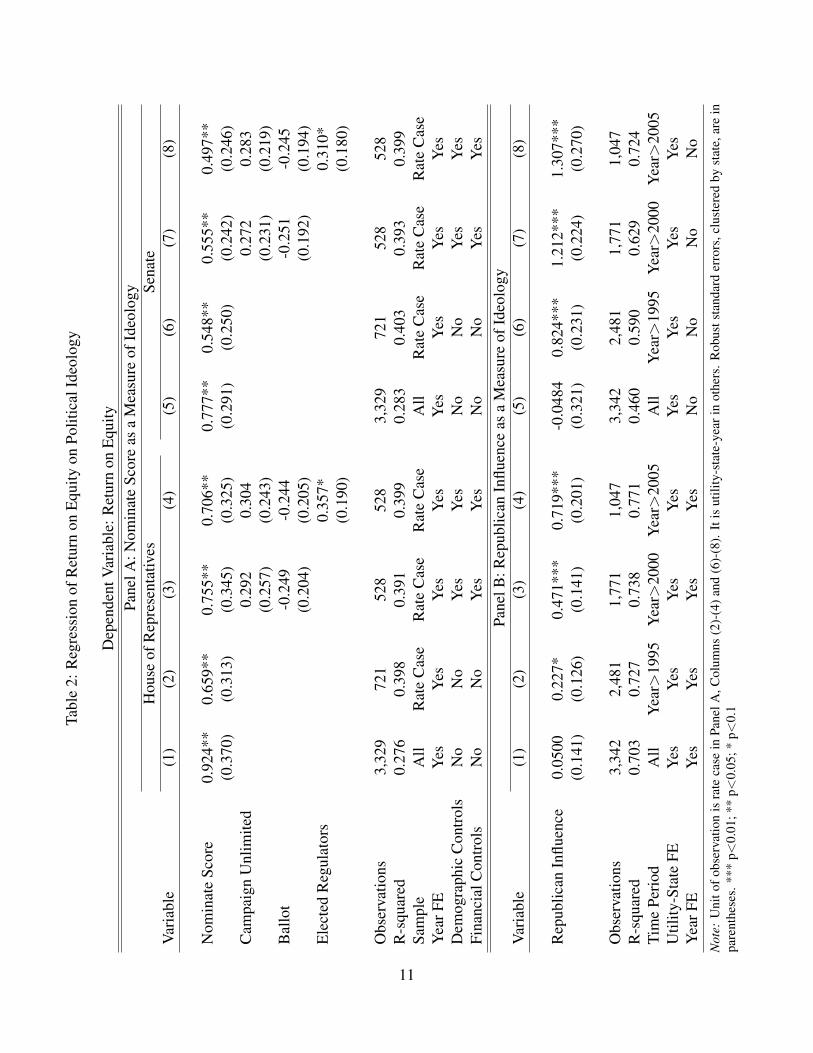
We first investigate the relationship between political ideology of the state and the return on equityapproved in rate cases.19 Figure 1 shows scatter plots of return on equity and Nominate scores for

exact definitions vary over time and across utilities.17SAIDI is equal to the sum of all customer interruption durations divided by the total number of customers. We

also have System Average Interruption Frequency Index (SAIFI) and Customer Average Interruption Duration Index(CAIDI). SAIFI is equal to the total number of interruptions experienced by customers divided by the number ofcustomers, so that it does not account for duration of interruption. CAIDI is equal to SAIDI divided by SAIFI.It measures the average duration conditional on having an interruption. We use SAIDI as our default measure ofreliability as this measure includes both frequency and duration across all customers.

18The capital used by utilities to fund investments commonly comes from three sources: the sale of common stock(equity), preferred stock and bonds (debt). The weighted-average cost of capital, where the equity ratio is the weighton equity, becomes the rate of return on capital that a utility is allowed to earn. Thus, return on capital is a function ofreturn on equity and equity ratio. In the regressions in Section 2.3.1, we document results on return on equity, becausereturn on capital is a noisier measure of regulators’ discretion due to random variation in equity ratio.

19What we obtain in this analysis is a correlation rather than a precise causal relationship. However, it is reasonableto interpret our result as causal for several reasons. First, theoretically, equity ratio and bond rating are the two keyfactors that determine adjudication of the return on equity, and we control for them. Second, the return on equity isunlikely to influence the partisan composition of commissioners. In the states with appointed regulators, the electionof governors, who subsequently appoint regulators, is determined by other factors such as taxation or education ratherthan electricity pricing. Even in the states with elected regulators, the election of low-profile public officials such asregulators is determined primarily by partisan tides (see Squire and Smith (1988) or Lim and Snyder (2014)). Thus,reverse causality is not a serious concern. Third, compared with political institutions such as appointment or electionof regulators, political ideology is a more intrinsic characteristic of political environments. It is less likely to be driven

9

AR

AZ

CA

CO

CT

DE

FL

GA

HI

IAID

ILIN

KS

KY

LAMA

MD

ME

MIMN

MOMS

NCND

NH

NJ

NM

NV

NY

OH

OK

OR

PA

RI

SC

SD

TX

UTVAVT WA

WI

WVWY

-1.5

-1-.

50

.51

Re

turn

on

Eq

uity (

Re

sid

ua

l)

-.5 0 .5 1Nominate Score for House

AR

AZ

CA

CO

CT

DE

FL

GA

HI

IAID

ILIN

KS

KY

LAMA

MD

ME

MIMN

MO MS

NCND

NH

NJ

NM

NV

NY

OH

OK

OR

PA

RI

SC

SD

TX

UTVAVTWA

WI

WVWY

-1.5

-1-.

50

.51

Re

turn

on

Eq

uity (

Re

sid

ua

l)

-.5 0 .5 1Nominate Score for Senate

Figure 1: Relationship between Return on Equity and Political Ideology

U.S. House and Senate. For return on equity, we use the residual from filtering out the influence offinancial characteristics (equity ratio and bond rating) of utilities, the demographic characteristics(income level and population density) of their service area, and year fixed effects. Observationsare collapsed by state.20 Both panels of the figure show that regulators in states with conservativeideology tend to adjudicate high return on equity.

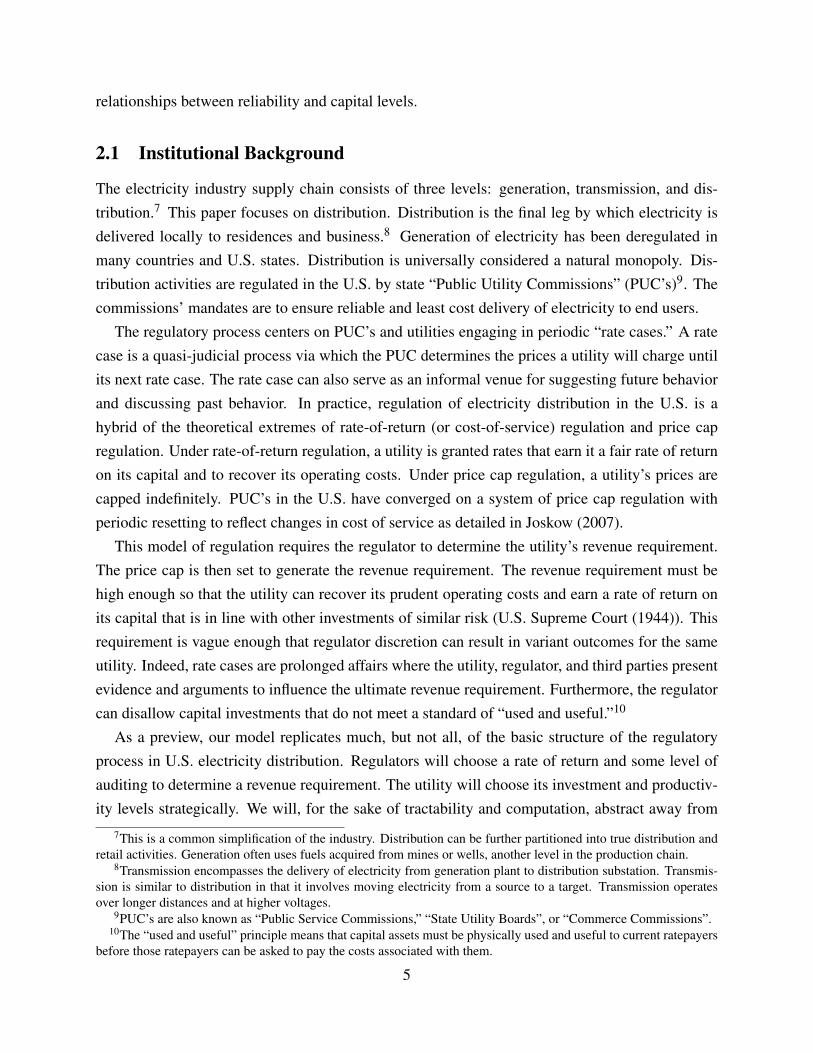
In Table 2 , we also present regressions of return on equity on Nominate score and other featuresof political environments21:

Return on Equityit = β1NominateScoreit +β2UnlimitedCampaigni +β3Balloti

+β4ElectedRegulatorsi +β5xit + γt + εit (1)

where UnlimitedCampaign, Ballot, and ElectedRegulators are dummy variables, xit is a vector ofdemographic and financial covariates for utility i in year t, and γt are year fixed effects.22

Panel A uses Nominate score for the U.S. House (Columns (1)-(4)) and Senate (Columns (5)-(8)) for the measure of political ideology. In Columns (1) and (5) of Panel A, we use all state-utility-year observations, without conditioning on whether it was a year in which rate case occurred

by characteristics of the energy industry in the state.20That is, we regress return on equity in each rate case on equity ratio, bond rating of the utilities, income level

and population density of their service area, and year fixed effects. Then, we collapse observations by state, and drawscatter plots of residuals and Nominate scores.

21In Section 1 of the supplementary material, we also document a sensitivity analysis of these regressions withrespect to variation in market structure (deregulation of wholesale and retail markets).

22Equation (1) above is the specification of Columns (4) and (8). Whether each variable is included or not variesacross specifications.

10

Tabl

e2:

Reg

ress

ion

ofR

etur

non

Equ

ityon

Polit

ical

Ideo

logy

Dep

ende

ntV

aria

ble:

Ret

urn

onE

quity

Pane

lA:N

omin

ate

Scor

eas

aM

easu

reof

Ideo

logy

Hou

seof

Rep

rese

ntat

ives

Sena

teV

aria

ble

(1)

(2)

(3)

(4)

(5)

(6)

(7)

(8)

Nom

inat

eSc

ore

0.92

4**

0.65

9**

0.75

5**

0.70

6**

0.77

7**

0.54

8**

0.55

5**

0.49

7**

(0.3

70)

(0.3

13)

(0.3

45)

(0.3

25)

(0.2

91)

(0.2

50)

(0.2

42)

(0.2

46)

Cam

paig

nU

nlim

ited

0.29

20.

304

0.27

20.

283

(0.2

57)

(0.2

43)

(0.2

31)

(0.2

19)

Bal

lot

-0.2

49-0

.244

-0.2

51-0

.245

(0.2

04)

(0.2

05)

(0.1

92)

(0.1

94)

Ele

cted

Reg

ulat

ors

0.35

7*0.

310*

(0.1

90)

(0.1

80)

Obs

erva

tions

3,32

972

152

852

83,

329

721

528

528

R-s

quar

ed0.

276

0.39

80.

391

0.39

90.

283

0.40

30.

393

0.39

9Sa

mpl

eA

llR

ate

Cas

eR

ate

Cas

eR

ate

Cas

eA

llR

ate

Cas

eR

ate

Cas

eR

ate

Cas

eY

earF

EY

esY

esY

esY

esY

esY

esY

esY

esD

emog

raph

icC

ontr

ols

No

No

Yes

Yes

No

No

Yes

Yes

Fina

ncia

lCon

trol

sN

oN

oY

esY

esN

oN

oY

esY

esPa

nelB

:Rep

ublic

anIn

fluen

ceas

aM

easu

reof

Ideo

logy

Var

iabl

e(1

)(2

)(3

)(4

)(5

)(6

)(7

)(8

)

Rep

ublic

anIn

fluen

ce0.

0500

0.22

7*0.

471*

**0.

719*

**-0

.048

40.

824*

**1.

212*

**1.

307*

**(0

.141

)(0

.126

)(0

.141

)(0

.201

)(0

.321

)(0

.231

)(0

.224

)(0

.270

)

Obs

erva

tions

3,34

22,

481

1,77

11,

047

3,34

22,

481

1,77

11,

047

R-s

quar

ed0.

703

0.72

70.

738

0.77

10.

460

0.59

00.

629

0.72

4Ti

me

Peri

odA

llY

ear>

1995

Yea

r>20

00Y

ear>

2005

All

Yea

r>19

95Y

ear>

2000

Yea

r>20

05U

tility

-Sta

teFE

Yes

Yes

Yes

Yes

Yes

Yes

Yes

Yes

Yea

rFE

Yes

Yes

Yes

Yes

No

No

No

No

Not

e:U

nito

fobs

erva

tion

isra

teca

sein

Pane

lA,C

olum

ns(2

)-(4

)and

(6)-

(8).

Itis

utili

ty-s

tate

-yea

rin

othe

rs.

Rob

usts

tand

ard

erro

rs,c

lust

ered

byst

ate,

are

inpa

rent

hese

s.**

*p<

0.01

;**

p<0.

05;*

p<0.

1

11

(henceforth “rate case year”). In Columns (2)-(4) and (6)-(8), we use only rate case years. Thestatistical significance of the relationship between return on equity and political ideology is robustto variation in the set of control variables. The magnitude of the coefficient is also fairly large.For example, if we compare Massachusetts, one of the most liberal states, with Oklahoma, oneof the most conservative states, the difference in return on equity due to ideology is about 0.61percentage points23, which is approximately 47% of the standard deviation in return on equity.24

Panel B uses Republican Influence, defined as the proportion of Republicans on the public util-ity commission, as the measure of political ideology. Columns (1) and (4) use the whole set ofutility-state-year observations. In other columns, we impose restrictions on data period. The resultshows an interesting cross-time pattern in the relationship between Republican Influence and re-turn on equity. In Columns (1) and (5), we do not find any significant relationship. However, as werestrict data to later periods, the coefficient of Republican Influence not only becomes statisticallysignificant, but its magnitude also becomes large. For example, Column (8) implies that replacingall-Democrat commission with all-Republican commission increases return on equity by 1.3 per-centage points in recent years (year>2005), which is approximately one standard deviation. Evenafter including year fixed effects, the magnitude is .7 percentage points (Column (4)).25 This find-ing that Republican Influence increases over time is consistent with ideological polarization in theU.S. politics, well documented in McCarty, Poole, and Rosenthal (2008). Using Nominate scores,they document that the ideological distance between the two parties has widened substantially overtime.26 Consistency between cross-time patterns of Republican Influence on return on equity andsubtle phenomena such as polarization adds a convincing piece of evidence on our argument thatpolitical ideology influences adjudication of rate cases.

We find that the influence of (no) restriction on campaign donation from corporations or theavailability of ballot propositions is not statistically significant. Considering that the skepticalview toward industry regulation by government in the public choice tradition has been primarilyfocused the possibility of “capture”, the absence of evidence on a relationship between return on

23If we collapse the data by state, Massachusetts has Nominate score for House around -.45, while Oklahoma has.42. Using the result in Column (4) in the upper panel, we get 0.706∗ (.42− (−.45))≈ 0.61.

24Once we filter out the influence of financial and demographic characteristics and year fixed effects, 0.61 percent-age points in this example is an even larger portion of variation. The residual in return on equity after filtering out thesecontrol variables has standard deviation 1.01. Therefore, the difference in return on equity between Massachusetts andOklahoma predicted solely by ideology based on our regression result is about .6 standard deviation of the residualvariation.

25In this context, not filtering out year fixed effects is more likely to capture the effect of political ideology moreaccurately. There can be nationwide political fluctuation that affects political composition of public service commis-sions. For example, if the U.S. president becomes very unpopular, all candidates from his party may have a seriousdisadvantage in elections. Thus, political composition of elected public service commission would be affected na-tionwide. Party dominance for governorship can be affected likewise, which affects composition of appointed publicservice commission. Including year fixed effects in the regression filters out this nationwide changes in the politicalcomposition of regulators, which narrows sources of identification.

26For details, see http://voteview.com/polarized america.htm.

12

equity and political institutions that can directly affect the extent of capture is intriguing.Our estimate implies that states with elected regulators are associated with higher level of profit

adjudicated for utilities, which contrasts with implications of several existing studies that use out-come variables different from rate of return. Formby, Mishra, and Thistle (1995) argue that electionof regulators is associated with lower bond ratings of electric utilities. Besley and Coate (2003)also argue that election of regulators helps to reflect voter preferences better than appointment,thus the residential electricity price is lower when regulators are elected.27

2.3.2 Return on Equity and Investment

To understand how political environments of rate regulation affect social welfare, we need to con-sider their effect on investment, which subsequently affects the reliability of electric power distri-bution. Thus, we now turn to the relationship between return on equity and investment.

We use two different measures of investment: the average yearly rate of addition to the value ofdistribution plant, gross of retiring plants (the first measure) and net of retiring plants (the secondmeasure). We take the average rate of addition to the distribution plant per year between rate caseyears as a proportion of the distribution plant in the preceding rate case year. We run regressionsof the following form:

Investmentit = αi +β1Return on Equityit +β2xit + εit

where Investmentit is the average yearly investment by utility i after rate case year t until the nextrate case, αi is utility-state fixed effects, Return on Equityit is the return on equity, and xit is a setof demographic control variables.

The result in Table 3 shows that there is a non-trivial, statistically significant relationship be-tween return on equity adjudicated in a rate case and subsequent investment by utilities. Forexample, Column (4) in Panel B shows that one percentage point increase in return on equity isassociated with .36 percentage point increase in the value of distribution plant, which is approx-imately a fifth of a standard deviation of net average yearly investment.28 The economic model

27Besley and Coate (2003) document that electing regulators is associated with electing a Democratic governor(Table 1 on page 1193). They do not include having a Democratic governor as an explanatory variable in the regressionof electricity price. Thus, the combination of the relationship between electing regulators and state-level politicalideology and our result that liberal political ideology yields low return on equity may explain the contrast betweentheir results and ours. Overall, our study differs from existing studies in many dimensions including data period,key variables, and econometric specifications. A thorough analysis of the complex relationship between various keyvariables used in existing studies and structural changes in the industry over time would be necessary to uncover theprecise source of the differences in results.

28Moreover, we can regard this relationship as a lower bound of the influence of rate of return on investment.Precisely, investment behavior is influenced by utility’s expectation of future rate of return rather than one from thepreceding rate case. Thus, the rate in the preceding rate case can be regarded as a proxy measure of the future rate ofreturn with a measurement error, i.e., a case of a right-hand-side variable with a measurement error.

13

Table 3: Regression of Investment on Return on Equity

Panel A: Average Yearly Rate of Addition to Distribution PlantVariable (1) (2) (3) (4)

Return on Equity 0.0023*** 0.0024*** 0.0031*** 0.0031***(0.0007) (0.0007) (0.0010) (0.0010)

Observations 510 509 510 509R-squared 0.030 0.033 0.440 0.439Utility-State FE No No Yes YesDemographic Controls No Yes No Yes

Panel B: Average Yearly Rate of Net Addition to Distribution PlantVariable (1) (2) (3) (4)

Return on Equity 0.0022** 0.0022*** 0.0036*** 0.0036***(0.0009) (0.0009) (0.0011) (0.0011)

Observations 510 509 510 509R-squared 0.017 0.031 0.384 0.384Utility-State FE No No Yes YesDemographic Controls No Yes No Yes

Note: Unit of observation is rate case. Robust standard errors, clustered by utility-state,in parentheses. *** p<0.01; ** p<0.05; * p<0.1

in Section 3 of a utility’s dynamic investment problem generates a positive correlation betweeninvestment and rates of return when regulator types are serially correlated.

2.3.3 Investment and Reliability

A utility’s reliability is partially determined by the amount of distribution capital and labor main-taining the distribution system. Our focus is on capital investment. Outages at the distribution levelresult from weather and natural disaster related damage29, animal damage30, tree and plant growth,equipment failure due to aging or overload, and vehicle and dig-in accidents (Brown (2009)). Cap-ital investments that a utility can take to increase its distribution reliability are putting power linesunderground, line relocation to avoid tree cover, installing circuit breaks such as re-closers, replac-ing wooden poles with concrete and steel, installing automated fault location devices, increasingthe number of trucks available for vegetation management31 and incident responses, and replacingaging equipment.

In Table 4, we examine how changes in capital levels affect realizations of reliability, by esti-

29Lightning, extreme winds, snow and ice, and tornadoes are the primary culprits of weather related damage.30Squirrels, racoons, gophers, birds, snakes, fire ants, and large mammals are the animals associated with outages.31Vegetation management involves sending workers to remove branches of trees which have grown close to power

lines so that they don’t break and damage the power line.

14

mating regressions of the form:

log(SAIDIit) = αi + γt +β1kit +β2lit +β3xit + εit

where SAIDIit measures outages for utility i in year t, kit is a measure of the utility i’s distributioncapital stock in year t, lit is utility i’s expenditures on operations and maintenance in year t, andxit is a vector of storm and terrain related explanatory variables. In this regression, there is mis-measurement on the left hand side, mis-measurement on the right hand side, and a likely correlationbetween ε shocks and expenditures on capital and operations and maintenance. Mis-measurementon the left hand side is because measurement systems for outages are imperfect. Mis-measurementon the right hand side arises by aggregating different types of capital into a single number basedon an estimated dollar value. The error term is likely to create a bias in our estimate of the effectof adding capital to reduce outages. We employ utility-state fixed effects, so that the variationidentifying the coefficient on capital is within utility-state over time.32 Even including utility-statefixed effects, a prolonged period of stormy weather would damage capital equipment and increaseoutage measures. The utility would compensate by replacing the capital equipment. Thus wewould see poor reliability and high expenditure on capital in the data. This correlation would causean upward bias in our coefficient estimates on β1 and β2, which reduces estimated sensitivity ofSAIDI to investment.33 Despite this potential bias, the result in Column (4), which is our preferredspecification, shows a strong negative relationship between capital investment and SAIDI.

2.3.4 Political Ideology and Utility Management (Energy Loss)

The preceding three subsections indicate one important channel through which political environ-ments influence social welfare: improvement of reliability under conservative commissioners be-cause higher returns lead to higher investment.34 On the other hand, conservatives’ favoritismtoward the utility relative to consumers implies a possibility that more conservative commission-ers may aggravate potential moral hazard by monopolists. To take a balanced view on this issue,we investigate the relationship between the political ideology of regulators and efficiency of utility

management. Our measure of static efficiency is how much electricity is lost during transmissionand distribution: energy loss. The amount of energy loss is determined by system characteristicsand actions taken by the utility’s managers to optimize system performance.

We find that conservative environments are associated with more energy loss. Table 5 presents

32Absent utility-state fixed effects, utilities in territories prone to outages would invest in more capital to preventoutages. This would induce a correlation between high capital levels and poor reliability.

33Recall that standard reliability measures of outage frequency and duration are such that lower values indicatemore reliable systems.

34In Section 4 of the supplementary material, we present an analysis of the direct (reduced-form) relationshipbetween the political ideology of regulators and reliability.

15

Table 4: Regression of Reliability Measure on Investment

Dependent Variable: Dependent Variable:SAIDI log(SAIDI)

Variable (1) (2) (3) (4)

Net Distribution Plant -9.92* -11.67*($ million) (5.28) (5.94)log(Net Distribution Plant) -0.272 -0.524***($ million) (0.170) (0.173)

Observations 1,687 1,195 1,684 1,192R-squared 0.399 0.663 0.744 0.769Utility-State FE Yes Yes Yes YesYear FE Yes Yes Yes Yes

O&M expense O&M expensesControls O&M expenseWeather

O&M expensesWeather

Note 1: Robust standard errors, clustered by state, in parentheses. *** p<0.01; ** p<0.05; * p<0.1Note 2 A higher value of SAIDI means lower reliability.

regressions of the following form:

log(energy lossit) = αi + γt +β1Republican In f luenceit +β2xit + εit

where xit is a set of variables that affect energy loss by utility i in year t, such as distribution capital,operation and management expenses, and the magnitude of sales.

The values for energy loss are non-trivial. The average amount of energy loss is 7% of totalproduction. In Panel A, we find that moving from all Republican commissioners to zero Republi-can commissioners reduces energy loss by 13%, which would imply 1 percentage point less totalenergy generated for the same amount of energy ultimately consumed.35 This is large. A back-of-the-envelope calculation for the cost of this 1% more electricity is 3.7 billion dollars per year.

We conclude that conservative political environment potentially encourages better reliabilitythrough higher return on equity and more investment, but it also leads to less static productivityas measured by energy loss. To conduct a comprehensive analysis of the relationship betweenpolitical environment and welfare from utility regulation, we now specify and estimate a modelthat incorporates both features.

35Panel B, based on Nominate score, yields a larger magnitude of the estimate. Since the analysis using Nominatescore is more subject to confounding factors (unobserved heterogeneity across utilities), we focus on the result fromPanel A. However, the consistency in the direction of the results between Panels A and B strengthens our interpretation.We also ran these specifications including peak energy demand to account for variance in load. The results are similarbut for a slightly lower magnitude of the Nominate score.

16

Table 5: Regression of Log Energy Loss on Political Ideology

Dependent Variable: log(energy loss)Panel A: Republican Influence as a Measure of Ideology

Variable (1) (2) (3) (4) (5) (6)

Republican Influence 0.169*** 0.118** 0.133** 0.133** 0.130** 0.130**(0.0538) (0.0550) (0.0580) (0.0590) (0.0592) (0.0592)

log(Net Distribution Plant) 0.483*** 0.460** 0.418** 0.418**(0.168) (0.173) (0.166) (0.166)

log(Operations and Maintenance) 0.0738 0.0586 0.0586(0.0775) (0.0778) (0.0778)

log(Sales) 0.221 0.221(0.143) (0.143)

Observations 3,286 3,286 3,276 3,276 3,263 3,263R-squared 0.906 0.908 0.908 0.908 0.909 0.909Utility-State FE Yes Yes Yes Yes Yes YesYear FE No Yes Yes Yes Yes YesWeather and Demographics No No No No No NoSample Restrictions Yes Yes Yes Yes Yes No

Panel B: Nominate Score as a Measure of IdeologyVariable (1) (2) (3) (4) (5) (6)

Nominate Score 1.025** 1.025** 0.516* 0.623** 0.609** 0.609**(0.448) (0.448) (0.277) (0.258) (0.255) (0.255)

log(Net Distribution Plant) 0.974*** 0.703*** 0.662*** 0.662***(0.0378) (0.106) (0.120) (0.120)

log(Operations and Maintenance) 0.306** 0.286** 0.286**(0.124) (0.119) (0.119)

log(Sales) 0.0717 0.0717(0.0538) (0.0538)

Observations 1,765 1,765 1,761 1,761 1,761 1,761R-squared 0.145 0.145 0.712 0.719 0.720 0.720Utility-State FE No No No No No NoYear FE Yes Yes Yes Yes Yes YesWeather and Demographics Yes Yes Yes Yes Yes YesSample Restrictions Yes Yes Yes Yes Yes No

Note 1: Unit of observation is utility-state-year. Robust standard errors, clustered by state, in parentheses. *** p<0.01;** p<0.05; * p<0.1Note 2: In columns (1)-(5) in each panel, we use the following sample restriction: 0.5 < efficiency < 1 whereefficiency = total sales

total sales+loss . We use this restriction to minimize the influence of outliers in the energy loss variable.

17

3 Model

We specify an infinite-horizon dynamic game between a regulator and an electric distribution util-ity. Each period is one year.36 The players discount future payoffs with discount factor β.

The state space consists of the value of utility’s capital k and the regulator’s weight on consumersurplus versus utility profits, α.37 Each period, the regulator chooses a rate of return on the utility’scapital base, r, and leniency of auditing, κ (κ ∈ [0,1]), or equivalently, audit intensity 1−κ. Afterthe utility observes the regulator’s choices, it decides how much to invest in distribution capitaland how much managerial effort to engage in for cost reduction.

Audit intensity is directly linked to materials cost pass-through rate. When regulators are max-imally lenient in auditing (κ = 1), i.e., minimally intense in auditing (1−κ = 0), they completelyreflect changes in material costs of electricity in consumer prices. It is an index of how high-powered the regulator sets the incentives for electricity input cost reduction.

The regulator’s weight on consumer surplus evolves exogenously between periods according toa Markov process. The capital base evolves according to the investment level chosen by the utility.We now detail the agents’ decision problems in terms of a set of parameters to be estimated anddefine the equilibrium notion.

3.1 Consumer Demand System

We assume a simple inelastic demand structure. An identical mass of consumers of size N are eachwilling to consume Q

N units of electricity up to a choke price p+ β log kN per unit:

D(p) =

{Q if p≤ p+ β log k

N

0 otherwise.

β is a parameter that captures a consumer’s preference for a utility to have a higher capital base. Allelse equal, a higher capital base per customer results in a more reliable electric system as demon-strated empirically in Table 4. This demand specification implies that consumers are perfectlyinelastic with respect to price up until the choke price. We make this simplifying assumption toeconomize on computational costs during estimation. Joskow and Tirole (2007) similarly assumeinelastic consumers in a recent theoretical study of electricity reliability. Furthermore, estimatedelasticities for electricity consumption are generally low, on the order of -0.05 to -0.5 (Bernsteinand Griffin (2005), Ito (2013)). Including a downward sloping demand function is conceptually

36In the data, rate case does not take place every year. For the years without a rate case in the data, we assume thatthe outcome of the hypothetical rate case in the model is the same as the previous rate case in the data.

37We will parameterize and estimate α as a function of the political environment.

18

simple, but slows down estimation considerably.38

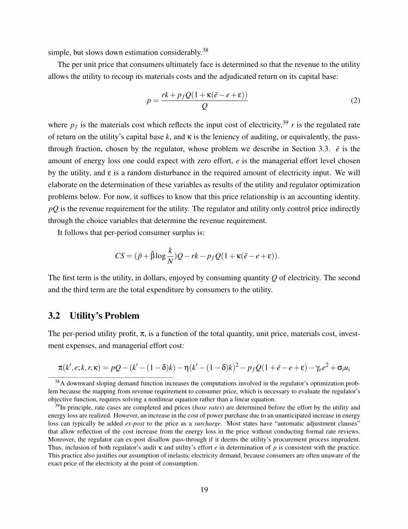
The per unit price that consumers ultimately face is determined so that the revenue to the utilityallows the utility to recoup its materials costs and the adjudicated return on its capital base:

p =rk+ p f Q(1+κ(e− e+ ε))

Q(2)

where p f is the materials cost which reflects the input cost of electricity,39 r is the regulated rateof return on the utility’s capital base k, and κ is the leniency of auditing, or equivalently, the pass-through fraction, chosen by the regulator, whose problem we describe in Section 3.3. e is theamount of energy loss one could expect with zero effort, e is the managerial effort level chosenby the utility, and ε is a random disturbance in the required amount of electricity input. We willelaborate on the determination of these variables as results of the utility and regulator optimizationproblems below. For now, it suffices to know that this price relationship is an accounting identity.pQ is the revenue requirement for the utility. The regulator and utility only control price indirectlythrough the choice variables that determine the revenue requirement.

It follows that per-period consumer surplus is:

CS = (p+ β logkN)Q− rk− p f Q(1+κ(e− e+ ε)).

The first term is the utility, in dollars, enjoyed by consuming quantity Q of electricity. The secondand the third term are the total expenditure by consumers to the utility.

3.2 Utility’s Problem

The per-period utility profit, π, is a function of the total quantity, unit price, materials cost, invest-ment expenses, and managerial effort cost:

π(k′,e;k,r,κ) = pQ− (k′− (1−δ)k)−η(k′− (1−δ)k)2− p f Q(1+ e− e+ ε)− γee2 +σiui

38A downward sloping demand function increases the computations involved in the regulator’s optimization prob-lem because the mapping from revenue requirement to consumer price, which is necessary to evaluate the regulator’sobjective function, requires solving a nonlinear equation rather than a linear equation.

39In principle, rate cases are completed and prices (base rates) are determined before the effort by the utility andenergy loss are realized. However, an increase in the cost of power purchase due to an unanticipated increase in energyloss can typically be added ex-post to the price as a surcharge. Most states have “automatic adjustment clauses”that allow reflection of the cost increase from the energy loss in the price without conducting formal rate reviews.Moreover, the regulator can ex-post disallow pass-through if it deems the utility’s procurement process imprudent.Thus, inclusion of both regulator’s audit κ and utility’s effort e in determination of p is consistent with the practice.This practice also justifies our assumption of inelastic electricity demand, because consumers are often unaware of theexact price of the electricity at the point of consumption.

19

where k′ is next period’s capital base, η is the coefficient on a quadratic adjustment cost in capital tobe estimated, δ is the capital depreciation rate, and γe is an effort cost parameter to be estimated. ui

is an investment-level-specific i.i.d. error term which follows a standard extreme value distributionmultiplied by coefficient σi.40 ui is known to the utility when it makes its investment choice,but the regulator only knows its distribution. η’s presence is purely to improve the model fit oninvestment. Such a term has been used elsewhere in estimating dynamic models of investment,e.g., in Ryan (2012).

Effort increases the productivity of the firm by reducing the amount of materials needed todeliver a certain amount of output. The notion of the moral hazard problem here is that the utilityexerts unobservable effort level e, the regulator observes the total energy loss which is a noisyoutcome partially determined by e, and the regulator’s “contract” for the utility is linear in thisoutcome. We assume effort is the only determinant of the materials cost other than the randomdisturbance, which implies that capital does not affect materials cost. Furthermore, effort does notreduce outages. While this separation is more stark than in reality, it is a reasonable modelingassumption for several reasons. The capital expenditures for reducing line loss – replacing theworst performing transformers – are understood to be small. In contrast, capital expenditures forimproving reliability, such as putting lines underground, fortifying lines, adding circuit breakersand upgrading substations, are large. As a result, empirically we can not estimate the beneficialimpact of capital expenditures on line loss as we do for reliability, and we do not include thisavenue in the theoretical model.41

The investment choice, k′− (1− δ)k, could also be written as a function of the regulator’searlier choices r and κ, but this is unnecessary. The optimal choice of k′ does not depend on κ

or this period’s r because neither the cost of investment nor the benefits of the investment dependon those choices. The benefits will depend on the future stream of r choices, but not this period’sr. Substituting the price accounting identity (equation (2) on page 19) into the utility’s per-periodpayoff function simplifies the payoff function to

π(k,k′,e,Q, p) = rk− (k′− (1−δ)k)−η(k′− (1−δ)k)2 +(κ−1)p f Q(e− e+ ε)− γee2 +σiui.

The utility’s investment level determines its capital state next period. The utility’s dynamicproblem is to choose effort and investment to maximize its expected discounted value:

vu(k,α) = maxk′,e

E[π(k,k′,e,r,κ)|ui]+βE[vu(k′,α′)|k,k′,e,r,κ,α].

40This error term is necessary to rationalize the dispersion in investment that is not explained by variation acrossthe state space.

41A similar argument holds for effort and reliability. In practice, the non-capital expenditures to improve reliabilitysuch as vegetation management are small relative to overall operations expenditures such that we can not estimatetheir effect.

20

The utility’s optimal effort choice has an analytical expression which we use in estimation:

e∗(κ) = min{−(κ−1)p f Q

2γe, e}

When κ is equal to one, which implies minimal audit intensity (1−κ = 0), the utility is reimbursedevery cent of electricity input expenses. Thus, it will exert zero effort. If κ is equal to zero, thenthe utility bears the full cost electricity lost in distribution. Effort is a function of the regulator’sauditing intensity because the regulator moves first within the period.

3.3 Regulator’s Problem

The regulator’s payoff is the geometric mean42 of expected discounted consumer welfare, or con-sumer value (CV)43, and the utility value function, vu, minus the cost of auditing and the cost ofdeviating from the market return:

uR(r,κ;α,k) = E[CV (r,κ,k,e)|r,κ]αE[vu(r,κ,k,e)|r,κ]1−α− γκ(1−κ)2− γr(r− rm)2

where α is the weight the regulator puts on consumer welfare against utility value, r is the regulatedrate of return, 1−κ is the auditing intensity, γκ is an auditing cost parameter to be estimated, rm

is a benchmark market return for utilities, and γr is an adjustment cost parameter to be estimated.CV is the value function for consumer surplus:

E[CV (r,κ,k,e)|r,κ] =∞

∑τ=t

βτ−tE[(p+ β log

kτ

N)Q− rτkτ− p f Q(1+κτ(eτ− eτ + ετ))|rt ,κt ]].

By default the utility is reimbursed for its total electricity input cost. The regulator incurs a cost fordeviating from the default of full pass-through: γκ(1−κ)2. The regulator must investigate, solicittestimony, and fend off legal challenges by the utility for disallowing the utility’s electricity costs.The further the regulator moves away from full pass-through, the more cost it incurs. This is aclassical moral hazard setup. Line loss is a noisy outcome resulting from the utility’s effort choice.The regulator uses a linear contract in the observable outcome, as in Holmstrom and Milgrom(1987), to incentivize effort by the utility.

The term γr(r− rm)2 is an adjustment cost for deviating from a benchmark rate of return suchas the average return for utilities across the country. A regulator who places all weight on utility

42An important principle in rate regulation is to render a non-negative economic profit to utilities, which is a type of“individual rationality condition”. The usage of geometric mean in this specification renders tractability of the modelin dealing with such condition, by ensuring non-negative value of the firm in the solution. This specification is alsoanalogous to the Nash bargaining model in which players maximize the geometric mean of their utilities.

43Consumer value is employed in dynamic models of merger regulation such as Mermelstein et al. (2012).

21

profits would not be able in reality to adjudicate the implied rate of return to the utility. Consumergroups and lawmakers would object to the supra-normal profits enjoyed by investors in the utilityrelative to similar investments. A regulator who places more weight on utility profits can increaserates by small amounts44, but only up to a certain degree.

The two terms, γκ(1− κ)2 and γr(r− rm)2, in the regulator’s per-period payoff are both dis-utility incurred by the regulator for deviating from a default action. Regulators with differentweights on utility profits and consumer surplus will deviate from these defaults to differing degrees.

We assume that the weight on consumer surplus is a function of political composition of thecommission and the political climate. Specifically,

α = a0 +a1rep+a2d

where rep is the fraction of Republican commissioners in the state, d is the Nominate score of theutility’s state, and the vector a≡ (a0,a1,a2) is a set of parameters to be estimated.

3.4 Equilibrium

We use the solution concept of Markov Perfect Equilibrium.

Definition. A Markov Perfect Equilibrium consists of

• Policy functions for the utility: k′(k,α,r,κ,ui) and e(k,α,r,κ,ui)

• Policy functions for the regulator: r(k,α) and κ(k,α)

• Value function for the utility: vu(k,α)

• Value function for consumer surplus (“consumer value”): CV (k,α)

such that

1. The utility’s policy function is optimal given its value function and the regulator’s policy func-

tions.

2. The regulator’s policy function is optimal given consumer value, the utility’s value function,

and the utility’s policy functions.

3. The utility’s value function and consumer value function are equal to the expected discounted

values of the stream of per-period payoffs implied by the policy functions.

3.5 Discussion of Game

There are two, somewhat separate, interactions between the regulator and the utility. The firstinvolves the investment choice by the utility and the rate of return choice by the regulator. Thesecond involves the effort choice by the utility and the audit intensity choice by the regulator.

44For example, the regulator can accept arguments that the utility in question is more risky than others.

22

In the first, the regulator and utility are jointly determining the amount of investment in thedistribution system. The regulator’s instrument in this dimension is the regulated rate of return. Inthe second, the utility can engage in unobservable effort which affects the cost of service by de-creasing the amount of electricity input need to deliver a certain amount of output. The regulator’sinstrument in this dimension is the cost pass-through, or auditing policy.

3.5.1 Investment, Commitment, and Averch-Johnson Effect

If the utility expects a stream of high rates of return, it will invest more. The regulator can notcommit to a path of returns, however. Therefore, the incentives for investment arise indirectlythrough the utility’s expectation of the regulated rates that the regulator adjudicates from period toperiod. This dynamic stands in contrast to the Averch-Johnson effect (Averch and Johnson (1962))whereby rate-of-return regulation leads to over-investment in capital or a distortion in the capital-labor ratio towards capital. The idea of Averch-Johnson is straightforward. If a utility can borrowat rate s, and earns a regulated rate of return at r > s, then the utility will increase capital. Thekey distinction in our model is that r is endogenously chosen by the regulator as a function of

the capital base to maximize the regulator’s objective function. r may exceed s at some states ofthe world, but if the utility invests too much, then r will be endogenously chosen below s. Thisfeature of the model might seem at odds with the regulatory requirement that a utility be allowedto earn a fair return on its capital. However, capital expenditures must be incurred prudently, andthe resulting capital should generally be “used and useful.” In our formulation, the discretion todecrease the rate of return substitutes for the possibility of capital disallowances when regulatorshave discretion over what is deemed “used and useful.”

3.5.2 Cost Pass-Through and Auditing

The costs of unobservable effort of finding qualified dispatchers and engineers, procuring electric-ity cost-effectively from nearby sources, and tracking down problems in the distribution networkthat are leading to loss are borne by the utility’s management. If the regulator accepts the costsassociated with energy loss without question, then the utility’s management has no incentive toexert unobservable effort. Thus, there is a moral hazard problem in the game between the regulatorand the utility. The regulator chooses how high powered to set the incentives for the utility to exertunobservable effort through the fraction of electricity input costs it allows the utility to recoup.45

45This friction in regulation is mentioned in regulatory proceedings and regulatory documents. For example,Hempling and Boonin (2008) states that “[cost pass-through mechanisms]... can produce disincentives for utilityoperational efficiency, since the clause allows the utility to recover cost increases, whether those cost increases arisefrom... (c) line losses.” This document goes on to assert that an effective pass-through mechanism should containmeaningful possibilities for auditing the utility’s operational efficiency to mitigate such concerns.

23

The regulator’s actions in both interactions are determined by its weight on consumer surplus.Intuitively, the utility likes high returns and weak auditing. Therefore, the more weight the regula-tor places on utility profits, the higher the rate of return it will regulate, and the less auditing it willengage in. We now turn to estimating the parameters of this game with a focus on the mappingbetween political environment variables to the regulator’s weight on consumer surplus.

4 Estimation

We estimate eight parameters: the effort cost parameter γe, the audit cost parameter γκ, the quadraticadjustment cost coefficient η, the market rate adjustment cost γr, the coefficient of the error termin the utility’s investment decision σi, and the mapping from political climate of the state and partyaffiliation of regulators to weight on consumer surplus versus utility profits, a ≡ (a0,a1,a2). Wedenote θ ≡ (γe,η,γκ,γr,σi,a). We fix the yearly discount factor of the players, β, at 0.96. We fixthe capital depreciation rate at 0.041.46 We set p f , the wholesale price of electricity, to $70 permegawatt-hour. We set e so that zero effort results in the utility losing one-third of its electricityinput cost in distribution.

We use a sub-sample of the data for estimation. We excluded utilities with less than 50,000customers or whose net distribution capital per customers exceeds $3,000. These outlier utilitiesare mostly in the Mountain West and Alaska. The population density and terrain of these utilitiesare sufficiently different from the bulk of U.S. electric distribution utilities that we do not want tocombine them in the analysis. We also excluded utility-years where the energy loss exceeds 15% orthe absolute value of the investment rate exceeds 0.1. The energy loss criterion eliminates aroundtwenty observations.47 The investment restriction is to deal with acquisitions and deregulationevents. Our final sample is 2331 utility-state-year observations, just above two-thirds of the fullsample of utility-state-years with the bulk of the difference being from dropping small utilities.

4.1 Demand Parameters: Value of Reliability

We calibrate the demand parameters so that the willingness-to-pay of the representative consumerfor a year of electricity service at the average capital level in the data is $24,000.48 We set thewillingness-to-pay for improving reliability, as measured by SAIDI, by one minute to $2.488 per

46This is the average level in our data computed from FERC Form 1 Depreciation Expense and the IRS MACRSdepreciation rate for electric distribution capital.

47The implied energy loss values are unreliable in these cases because they are derived from utility territories whichoperate in multiple states, but report one aggregate level of energy loss.

48The $24,000 number is somewhat arbitrary as we are not modeling whether the consumer is residential, commer-cial, or industrial, nor can one reliably elicit this number. Adjusting this value will have a direct effect on the estimatedlevel of a0, but is unlikely to affect other results in this paper.

24

customer per year. The choice of the value of reliability has first order implications for the coun-terfactual analysis that we perform. We estimated this number using the results of LaCommareand Eto (2006) who use survey data to estimate the cost of power interruptions. Estimated valuesfor improvements in reliability are heterogenous by customer class, ranging from $0.5-$3 to avoida 30 minute outage for residential consumers to $324-$435 for small commercial and industrialconsumers to $4,330-$9,220 for medium to large commercial and industrial consumers.49 To getto $2.488 per minute of SAIDI per customer per year, we use the mid-point of the estimates bycustomer class, and set 0.38 percent of consumers to medium to large commercial and industrial,12.5 percent to small commercial and industrial, and the remaining 87.12 percent to residential.50

From these values, a crude calculation for the level of under-investment is derived as follows.The net present value of $2.488 per minute per customer per year is $62.224 per minute per cus-tomer at a discount factor of 0.96. The reliability on capital regression implies that the one-time,per-customer change in the capital base required to improve SAIDI by one minute is $34.432 forthe mean utility. The benefit exceeds the cost such that moderate decreases in the benefit wouldstill be consistent with under-investment. Our model improves the credibility of this crude calcu-lation by including depreciation, future investment, and investment costs not captured by the bookvalue of the assets.51

4.2 Regulator and Utility Parameters

We estimate the parameters in θ using a two-step procedure for dynamic games following Bajariet al. (2007) (BBL) and Pakes et al. (2007). This method avoids computationally costly re-solvingof the equilibrium. The estimation objective evaluates candidate sets of parameters by simulatingvalue functions implied by those parameters and the observed policies in the data, and comparingthe observed policies to those which are optimal given the simulated value functions and candidateparameters. Our problem has two features which are non-standard. First, the effort and regulatoryauditing policies are unobserved.52 Second, one of the state variables, the regulator’s weight onconsumer surplus is not observed directly. The solution in both cases is to derive the unobservedquantity as a function of model parameters and data.

49While some of these customers may have back-up generation, that is rarely enough to support full operation ofthe plant during the outage. For example, a hospital might back-up enough power to keep treating its current patients,but divert new emergency room patients to another hospital, or cancel non-urgent outpatient procedures.

50The survey measures for willingness-to-pay to improve reliability are fraught with issues such as truthful elicita-tion and aggregating surveys with differently phrased questions. Accordingly, we later assess robustness of our resultsto these values.

51We assume no heterogeneity in these values and costs. If the value of reliability is positively correlated with thecost of improving reliability, then this calculation is no longer valid. Our data on reliability were not rich enough tomeasure heterogenous costs of improving reliability.

52Unobserved effort is a challenge in the empirical analysis of moral hazard problems (Misra and Nair (2011),Lewis and Bajari (2013)).

25

The data are, for every utility-state (i) and year (t): a capital base kit , an investment level invit ,realized energy loss lit in MWh, a return on capital rit , a market size Qit in MWh, a fraction ofRepublican utility commissioners repit , and a state Nominate score dit . The following list describesthe steps for calculating the estimation objective function for a given set of model parameters θ.We then detail each step:

Estimation Steps1. Consider candidate model parameters θ = (γe,η,γκ,γr,σi,a).2. Transform political data into weights on consumer surplus using a. Estimate a Markov process

for weight on consumer surplus.3. Transform energy loss into unbiased estimates of effort and audit intensity using γe and first

order condition for optimal effort.4. Estimate policy functions for investment, effort, rate of return, and audit intensity.5. Simulate value functions implied by θ and estimated policy functions.6. Solve for optimal policies given by implied value functions and θ.7. Compute moments implied by optimal policies and Markov process for weight on consumer

surplus.8. Calculate objective function.

We discretize the state space into a grid of points for capital level and weight on consumersurplus level. We first transform the data on the fraction of Republican commissioners and theNominate score of a state into an implied weight on consumer surplus by αit = a0+a1repit +a2dit .This resolves the issue of one dimension of the state space being unobserved. We use the impliedαit series to approximate a first-order Markov process for the weight on consumer surplus over thediscretized grid.

Next, we invert energy loss lit into an unbiased estimate of effort according to the model. First,lit is equal to electricity procured minus electricity delivered:

lit = Qit(1+ e− eit + εit)−Qit .

We assume that εit has mean zero. It follows that

eit = e− litQit

.

eit is regressed on functions of state variables to produce an estimated effort policy function. Theestimation error due to eit being different from eit does not change the asymptotic properties of thisstep.53 We assume the utility serves Q units of energy every period, where Q is the mean of Qit

53The residual from this policy function estimation does affect the value function estimates in theory, but in practice26

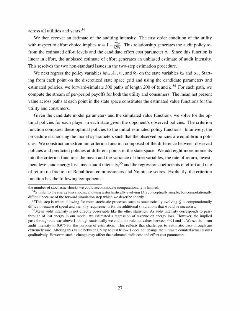
across all utilities and years.54

We then recover an estimate of the auditing intensity. The first order condition of the utilitywith respect to effort choice implies κ = 1− 2γee

Qp f. This relationship generates the audit policy κit

from the estimated effort levels and the candidate effort cost parameter γe. Since this function islinear in effort, the unbiased estimate of effort generates an unbiased estimate of audit intensity.This resolves the two non-standard issues in the two-step estimation procedure.

We next regress the policy variables invit , eit ,rit , and κit on the state variables kit and αit . Start-ing from each point on the discretized state space grid and using the candidate parameters andestimated policies, we forward-simulate 300 paths of length 200 of α and k.55 For each path, wecompute the stream of per-period payoffs for both the utility and consumers. The mean net presentvalue across paths at each point in the state space constitutes the estimated value functions for theutility and consumers.

Given the candidate model parameters and the simulated value functions, we solve for the op-timal policies for each player in each state given the opponent’s observed policies. The criterionfunction compares these optimal policies to the initial estimated policy functions. Intuitively, theprocedure is choosing the model’s parameters such that the observed policies are equilibrium poli-cies. We construct an extremum criterion function composed of the difference between observedpolicies and predicted policies at different points in the state space. We add eight more momentsinto the criterion function: the mean and the variance of three variables, the rate of return, invest-ment level, and energy loss, mean audit intensity,56 and the regression coefficients of effort and rateof return on fraction of Republican commissioners and Nominate scores. Explicitly, the criterionfunction has the following components:

the number of stochastic shocks we could accommodate computationally is limited.54Similar to the energy loss shocks, allowing a stochastically evolving Q is conceptually simple, but computationally

difficult because of the forward simulation step which we describe shortly.55This step is where allowing for more stochastic processes such as stochastically evolving Q is computationally

difficult because of speed and memory requirements for the additional simulations that would be necessary.56Mean audit intensity is not directly observable like the other statistics. As audit intensity corresponds to pass-

through of lost energy in our model, we estimated a regression of revenue on energy loss. However, the impliedpass-through rate was above 1, though statistically we could not rule out values between 0.91 and 1. We set the meanaudit intensity to 0.975 for the purpose of estimation. This reflects that challenges to automatic pass-through areextremely rare. Altering this value between 0.9 up to just below 1 does not change the ultimate counterfactual resultsqualitatively. However, such a change may affect the estimated audit cost and effort cost parameters.

27

G(θ) =

1Nk,α

∑k,α inv(k,α)− înv(k,α;θ)

1Nk,α

∑k,α e(k,α)− e(k,α;θ)

1Nk,α

∑k,α r(k,α)− r(k,α;θ)

1Nk,α

∑k,α κ(k,α)− κ(k,α;θ)

1NT ∑

Ni=1 ∑

Tt=1 rit− ˆr(θ)

1NT ∑

Ni=1 ∑

Tt=1(rit− r)2− σ2

r (θ)1

NT ∑Ni=1 ∑

Tt=1 invit− înv(θ)

1NT ∑

Ni=1 ∑

Tt=1(invit− ¯inv)2− σ2

inv(θ)1

NT ∑Ni=1 ∑

Tt=1 eit− ê(θ)

1NT ∑

Ni=1 ∑

Tt=1(eit− e)2− σ2

e(θ)1

NT ∑Ni=1 ∑

Tt=1 κit− ˆκ(θ)

βe,data− βe(θ)

βr,data− βr(θ)

where x for policy x denotes the optimal choice implied by the model at the candidate parametersθ. We minimize the weighted sum of squares of G(θ):

θ = argminθ

G(θ)′WG(θ)

where W is a weighting matrix. The first four components of G(θ) are the differences betweenobserved policies and implied optimal policies averaged across points in the state space. Thenext seven components are the mean and the variance of outcomes.57 The final two componentscompare regression coefficients from the data to regression coefficients implied by the model.We match two regressions: regulated rate of return on Nominate score and fraction of republicancommissioners, and effort on Nominate score and fraction of republican commissioners. We set theweighting matrix W to adjust for differences in scaling across moments. We compute confidenceintervals by block-bootstrap, clustering by utility-state.

5 Estimation Results

In this section, we interpret the economic magnitude of parameter estimates and discuss the em-pirical identification of the parameters. Table 6 shows the estimation results.Magnitudes and Model Fit: The effort cost parameter, γe, implies that decreasing energy loss by1% at the mean effort would entail a disutility worth about $284,000 to utility management. Thisis comparable to the cost of hiring one to two power system engineers. The adjustment cost for

57As the parameter vector a affects transitions across states, these moments are not implied by matching observedpolicies to implied optimal policies state by state.

28

Table 6: Parameter Estimates

95%-CI 95%-CIParameter Related Model Component EstimateLower-bound Upper-bound

γe(107) effort cost 5.8504 5.2900 6.6613γκ(1010) audit cost 17.4760 13.4229 21.0956γr(1010) market return adjustment cost 2.8868 2.0778 9.1118

η(104) quadratic investment cost 11.2177 5.9422 22.3227σi(107) investment-level-specific error 2.4146 1.0069 8.6828

a0 weight on consumer surplus 0.9998 0.9971 1.0052a1 weight on consumer surplus -0.0046 -0.0211 -.0005a2 weight on consumer surplus -0.0019 -.0020 0.0012N 2331

Criterion 0.0006335

capital, η, is small relative to the actual cost of capital, that is, the linear term in investment. Fora 10% investment from the mean capital level, the adjustment cost is equal to 14.87% of the costof the capital itself. This parameter is likely picking up heterogeneity across utilities not specifiedin the dynamic model, such as population growth rates and idiosyncratic features of the terrain.The regulator’s cost parameters, γr and γκ, imply that adjusting the rate of return by one standarddeviation in the data (1.3 percentage points) from the mean bears the same cost as decreasing costpass-through rate by 0.1 percentage points from the mean (97.5% to 97.4%).

The mapping from political variables to weight on consumer surplus describes regulator het-erogeneity. a0 sets the level of weight on consumer surplus. It is very close to one. This reflectsthat current electricity prices are a very small fraction of willingness-to-pay for electricity. Thevalue is sensitive to the calibration of willingness-to-pay for electricity, described on page 24. a1

is larger in magnitude than a2. Both are negative implying that more conservative areas, whethermeasured by Nominate scores or fraction of republican commissioners, place relatively less weighton consumer surplus than liberal areas, leading to higher rates of return and more energy loss.

In Figure 2, we plot the policy surfaces at the estimated parameters for investment and rateof return as functions of capital per capita and the weight on consumer surplus. Both the rate ofreturn and investment are decreasing in the two dimensions. Investment decreases in the weighton consumer surplus because of persistence in the stochastic process of the weight. In Figure 3,we plot all of the policy functions at the estimated parameters, averaged across levels of capital, inthe dimension of weight on consumer surplus. Auditing is increasing in the weight on consumersurplus, which implies that effort is also increasing in this dimension.

In terms of model fit, the estimated model does well matching the first moments of the keychoice variables. While the model predicts the variance of investment well, it does not fit thevariance of energy loss nor rate of return well. There are clear reasons for this. Investment is

29

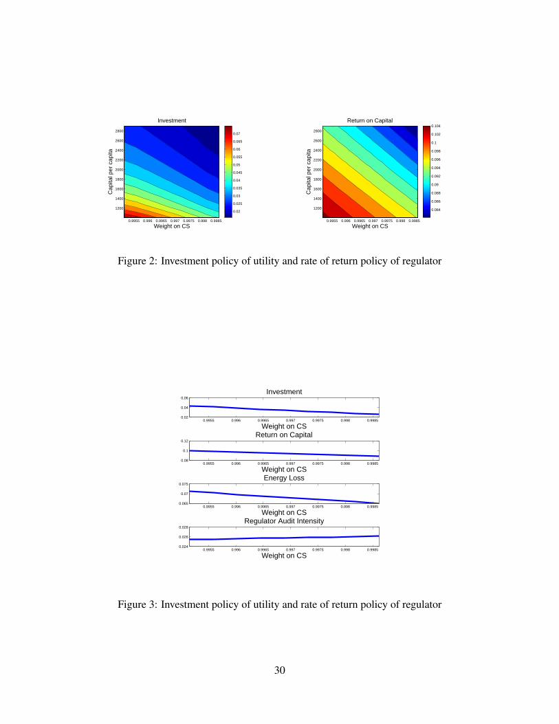
Investment

Cap

ital p

er c

apita

Weight on CS

0.9955 0.996 0.9965 0.997 0.9975 0.998 0.9985

1200

1400

1600

1800

2000

2200

2400

2600

2800

0.02

0.025

0.03

0.035

0.04

0.045

0.05

0.055

0.06

0.065

0.07

Return on Capital

Cap

ital p

er c

apita

Weight on CS

0.9955 0.996 0.9965 0.997 0.9975 0.998 0.9985

1200

1400

1600

1800

2000

2200

2400

2600

2800

0.084

0.086

0.088

0.09

0.092

0.094

0.096

0.098

0.1

0.102

0.104

Figure 2: Investment policy of utility and rate of return policy of regulator

0.9955 0.996 0.9965 0.997 0.9975 0.998 0.99850.02

0.04

0.06Investment

Weight on CS

0.9955 0.996 0.9965 0.997 0.9975 0.998 0.99850.08

0.1

0.12Return on Capital

Weight on CS

0.9955 0.996 0.9965 0.997 0.9975 0.998 0.99850.065

0.07

0.075Energy Loss

Weight on CS

0.9955 0.996 0.9965 0.997 0.9975 0.998 0.99850.024

0.026

0.028Regulator Audit Intensity

Weight on CS

Figure 3: Investment policy of utility and rate of return policy of regulator

30

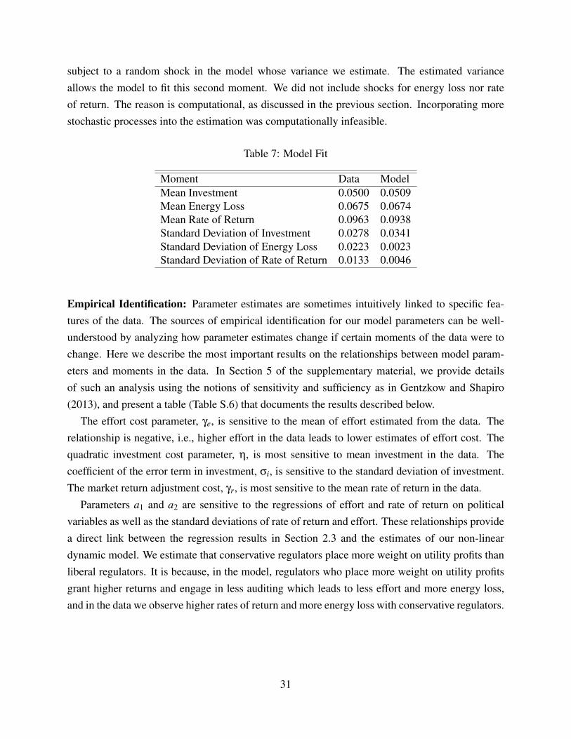
subject to a random shock in the model whose variance we estimate. The estimated varianceallows the model to fit this second moment. We did not include shocks for energy loss nor rateof return. The reason is computational, as discussed in the previous section. Incorporating morestochastic processes into the estimation was computationally infeasible.

Table 7: Model Fit

Moment Data ModelMean Investment 0.0500 0.0509Mean Energy Loss 0.0675 0.0674Mean Rate of Return 0.0963 0.0938Standard Deviation of Investment 0.0278 0.0341Standard Deviation of Energy Loss 0.0223 0.0023Standard Deviation of Rate of Return 0.0133 0.0046

Empirical Identification: Parameter estimates are sometimes intuitively linked to specific fea-tures of the data. The sources of empirical identification for our model parameters can be well-understood by analyzing how parameter estimates change if certain moments of the data were tochange. Here we describe the most important results on the relationships between model param-eters and moments in the data. In Section 5 of the supplementary material, we provide detailsof such an analysis using the notions of sensitivity and sufficiency as in Gentzkow and Shapiro(2013), and present a table (Table S.6) that documents the results described below.

The effort cost parameter, γe, is sensitive to the mean of effort estimated from the data. Therelationship is negative, i.e., higher effort in the data leads to lower estimates of effort cost. Thequadratic investment cost parameter, η, is most sensitive to mean investment in the data. Thecoefficient of the error term in investment, σi, is sensitive to the standard deviation of investment.The market return adjustment cost, γr, is most sensitive to the mean rate of return in the data.

Parameters a1 and a2 are sensitive to the regressions of effort and rate of return on politicalvariables as well as the standard deviations of rate of return and effort. These relationships providea direct link between the regression results in Section 2.3 and the estimates of our non-lineardynamic model. We estimate that conservative regulators place more weight on utility profits thanliberal regulators. It is because, in the model, regulators who place more weight on utility profitsgrant higher returns and engage in less auditing which leads to less effort and more energy loss,and in the data we observe higher rates of return and more energy loss with conservative regulators.

31

6 Counterfactual Experiments

We perform three sets of counterfactual experiments: (1) alternative rate of return policies by theregulator, including endowing the regulator with a commitment device, (2) alternative auditingpolicies for the regulator, and (3) alternative regulatory commission design, including minorityparty representation. In the first set, we explore a full commitment benchmark and setting therate of return policy equal to the most conservative regulator’s policy. In the second, we exploremaximal auditing by the regulator and setting the audit policy equal to the most liberal regulator’spolicy. Thus, each set explores a theoretical benchmark and partisan extreme. The key intuitionis that conservative environments reduce the problem of time inconsistency, while liberal envi-ronments reduce the problem of asymmetric information. Finally, in the third set, we exploreenforcing minority representation which limits the degree to which a commission can swing to onepartisan extreme or the other, and a perfectly centrist commission.

6.1 Rate of Return Policies including Commitment

As a theoretical benchmark, we solve for the regulator’s optimal policy when it can credibly com-mit to future rates of return. This idea is analogous to Taylor’s rule on monetary policy (Taylor(1993)), which stipulates the amount of change in the nominal interest rate in response to changesin inflation and output. Theoretically, commitment should lead to higher rates of return and higherinvestment by overcoming the fear of regulatory hold-up. Our results in Table 8 confirm and quan-tify the importance of this intuition.

We model commitment by changing the timing of actions in the dynamic game. In the com-mitment counterfactual, the regulator first chooses a rate of return policy that specifies r in eachstate (k,α). This policy is then held fixed. The utility solves a single agent problem conditional onthis policy. To make this problem computationally tractable, we constrained the regulator’s prob-lem so that their commitment policy must be a scalar multiple of their equilibrium policy from theestimated MPE. Furthermore, we hold the audit policy fixed at the estimated equilibrium audit pol-icy. These two restrictions reduce the commitment problem to a single dimensional optimizationproblem. We evaluate the commitment policy by averaging over different regulator preferencesaccording to the ergodic distribution implied by the estimated Markov process for α.

In a world where the regulator could credibly commit to future rates of return (“Full Com-mitment”), the adjudicated rate of return is 14 percent higher than in the baseline. In every state,investment rises substantially.58 The steady state mean capital level rises by 59%. Mean investment

58In Table 8, Investment w.r.t. Baseline is the un-weighted mean ratio of investment across states. The steady statemeans of investment (row 6) for baseline and commitment are closer to each other because the steady state capital ishigher under commitment, and investment is decreasing in capital.

32

Table 8: Results of Rate of Return Counterfactual Experiments

Baseline Conservative Rate Full Commitment∆ % ∆ %

Mean Return on Capital 0.100 0.103 3.24% 0.108 8.36%Return Policy w.r.t. Baseline 1.000 1.062 6.20% 1.140 14.00%

SD Return on Capital 0.003 0.001 -55.57% 0.004 15.79%Mean Audit 0.974 0.974 -0.01% 0.974 -0.01%

SD Audit 0.000 0.000 -3.20% 0.000 -14.01%Mean Investment Rate 0.052 0.056 7.62% 0.051 -2.93%

SD Investment Rate 0.007 0.007 5.96% 0.006 -8.46%Investment Policy w.r.t. Baseline 1 1.308 30.80% 1.459 45.90%

Mean Energy Loss 0.069 0.068 -0.92% 0.068 -1.09%SD Energy Loss 0.002 0.002 -3.20% 0.002 -14.01%

Utility Value Per Capita 1616.012 2131.540 31.90% 2981.877 84.52%Consumer Value Per Capita 539558.700 539619.620 0.01% 539291.004 -0.05%

Total Welfare 541174.712 541751.160 0.11% 542272.882 0.20%Steady State Capital Per Capita 1179.306 1462.226 23.99% 1880.266 59.44%

SAIDI (average outages) 144.687 134.416 -7.10% 119.240 -17.59%

Note: Different rates of change (∆%) in summary statistics can be associated with seemingly identical num-bers due to round-up errors.

is lower than under the baseline because the system spends more time at higher capital levels, andinvestment is decreasing in capital. Consumers would pay higher prices and receive service witharound 25.4 fewer outage minutes per year, or an 18% improvement in reliability. Utility valueincreases dramatically while consumer value slightly decreases. That consumer value decreases isnatural when thinking about commitment. Under commitment, the regulator finds itself in statesof the world where it would like to decrease the rate of return to increase consumer surplus, as itwould in a Markov Perfect Equilibrium.59

The main driver of this result (commitment increasing capital) is that the possible improvementsin reliability from capital additions are cheap compared to the their estimated benefit at currentcapital levels. When the regulator can commit to future policies, it can induce the utility to investup to the point where the marginal benefit of investment in reliability improvements equals themarginal cost of investment in capital. While there are not heterogenous types of capital in ourmodel, under-investment can be understood as a combination of too much aging infrastructurewhich has not been replaced and too little investment in new technologies such as automatedswitching systems.60

59That consumer welfare decreases slightly may also be driven by our restriction to regulator policies which are ascalar multiple of the Markov Perfect Equilibrium policy.

60We have abstracted from investments by distribution utilities in new technologies, such as accommodating dis-

33

Higher rates and investment do not occur in the Markov Perfect Equilibrium because of thefear of regulatory hold-up. Absent commitment by the regulator, the utility won’t make largeinvestments because once the investments are sunk, the regulator’s incentives lead to adjudicatinglow rate of return which do not adequately compensate the utility for the investments. Realizingthis incentive for regulatory hold-up, the utility does not invest in the first place. Such anticipationby the utility implies that regulatory hold-up can be a real impediment to welfare without one everobserving actual instances of large investments followed by decreases in regulated rates.

Actions that the government can take in reality for commitment include passing legislation forlarge investment programs. For example, the legislature in Illinois enacted legislation in 2011 toforce the regulator to pay a return on new investments in the electricity distribution infrastructure.The Energy Infrastructure Modernization Act in Illinois authorized $2.6 billion in capital invest-ment for Commonwealth Edison, the electricity distributor in Chicago. One of the main explicitgoals is reducing SAIDI by 20 percent, which is close to our model’s predicted reliability improve-ment under commitment. Commonwealth Edison praised the act as “[bringing greater stability tothe regulatory process to incent investment in grid modernization.” (McMahan (2012)). In Mis-souri, the Infrastructure Strengthening and Regulatory Streamlining Act was proposed with thesame justification. This legislation would have required Ameren Missouri to increase its capitalbase by 14.5% targeted at capital investments that improve distribution reliability. These legisla-tive initiatives bypass the traditional regulatory process conducted by rate cases with a more rigidlegislative regulatory process.

The implied magnitudes in this counterfactual are sensitive to the value of reliability. However,the qualitative outcome that regulated rates of return and investment are too low is not. In Section2 of the supplementary material, we tabulate how changes in the estimated value of reliability andchanges in the estimated cost of improving reliability by capital investment would approximatelyaffect the degree of estimated under-investment.61 If either the aggregate value of reliability im-provements from observed levels were half of the estimated value, or if the coefficient we estimatein the reliability-capital regression were two-thirds the estimated value, then we would estimatethat the average electricity distribution system has the appropriate capital level.

In “Conservative Rate” in Table 8, we constrain regulators to choose rates of return equal to orgreater than those chosen by the most conservative regulator. This constraint binds in all states,so equilibrium rates of return are equal to those of the most conservative regulator. Interestingly,this policy does slightly better than the constrained full commitment policy on consumer welfare,though the results are similar. Recall our full commitment policy is constrained to be a scalar

tributed generation from household solar power or installation of smart-meters whose major benefits do not arise fromreliability improvements.

61We vary the fraction of industrial consumers and commercial consumers, the corresponding valuations of thoseconsumers for improvements in reliability, and the technological rate at which capital improves reliability. The resultson under-investment are robust to moderate to large changes in these estimates.

34

Table 9: Results of Auditing Policy Counterfactual Experiments

Baseline Most Liberal Maximal Audit∆ % ∆ %

Mean Return on Capital 0.100 0.100 -0.09% 0.100 -0.03%SD Return on Capital 0.003 0.003 1.83% 0.003 2.66%

Mean Audit 0.974 0.974 -0.04% 0.967 -0.79%SD Audit 0.000 0.000 -96.92% 0.000 -100.00%

Mean Investment Rate 0.052 0.052 -0.16% 0.052 -0.10%SD Investment Rate 0.007 0.007 1.20% 0.007 1.59%Mean Energy Loss 0.069 0.065 -5.22% 0.000 -100.00%

SD Energy Loss 0.002 0.000 -96.92% 0.000 -100.00%Utility Value Per Capita 1616.012 1609.517 -0.40% 1602.792 -0.82%

Consumer Value Per Capita 539558.700 539734.130 0.03% 543068.318 0.65%Total Welfare 541174.712 541343.647 0.03% 544671.110 0.65%

Note: Different rates of change (∆%) in summary statistics can be associated with seemingly identicalnumbers due to round-up errors.

multiple of the MPE rate of return policy. Because of different regulator political ideologies, theMPE rate of return policy assigns different rates of return for the same capital level dependingon the commission make-up. The minimum rate of return policy eliminates these distortions.The results indicate that tilting towards a conservative regulator in areas with poor reliability is apossible substitute for commitment policies.

6.2 Auditing Policies

We now switch focus to the problem of asymmetric information which manifests itself as energyloss. In Table 9, we consider a uniform implementation of the maximum audit intensity estimatedfrom our data (“Most Liberal Audit”).62 We also consider the theoretical benchmark of maximalaudit policy (“Maximal Audit”) which maximally incentivizes the utility to reduce energy loss.

Under the audit policy set at the most liberal regulator’s level, energy loss decreases by aboutfive percent (half a percentage point of the total energy distributed). This implies that society couldconsume the same amount of electricity with half a percentage point less generation, saving on theorder of 1 billion dollars per year. Maximal auditing leads to zero energy loss. The utility is worseoff as it suffers a dis-utility from maximum effort. However, the improvement in consumer value

62In theory, there is no obvious linkage between the audit intensity in our model and specific auditing practices.However, the most stringent auditing practices could be studied and replicated. For example, the government can setup a rule by which the regulatory commission is required to allocate a certain amount of budget in monitoring utilitybehavior in power procurement.

35

dominates the loss in utility profits. As a result, total welfare increases.63

6.3 Commission Design and Minority Representation

Let us now consider imposing a restriction on the influence of politics in regulation. Specifically,we consider a rule which requires that no more than a certain fraction of regulatory commissionerscan be from the same party. This rule is already in place in some states. The bound is typically threecommissioners out of five. For example, in Connecticut, no more than three among five can be fromthe same political party; in Colorado, no more than two among three can be from the same politicalparty. We simulate such a rule (“Minority Representation”) with a mean-preserving shrinkage

of the Markov process governing the evolution of the regulator’s weight on consumer surplus.We reduce the standard deviation of the α process to 40% of the baseline which correspondsto the implied reduction in α if the fraction of Republican commissioners were bounded by 0.4and 0.6 in the data. Table 10 shows the results. By construction, this policy has little effecton mean outcomes. What determines the mean level of investment is the expected stream offuture returns which is not affected by this policy. However, this policy has a significant effecton second moments of rates of return and investment. Our result would be useful in designingand assessing policy tools to reduce variation in the quality and efficiency of energy distributionover time and across states.64 We also consider a regulatory commission at the mean with zerovariance as a theoretical benchmark (“Centrist Commission” in Table 10). The results are similarto the minority representation counterfactual, but with even greater decreases in the variance ofobservable outcomes.

6.4 Discussion: Commitment, Auditing, and Political Environments

Both time inconsistency and asymmetric information have quantitatively large effects on electricpower distribution. Time inconsistency leads to under-investment in capital. Asymmetric infor-mation leads to too much energy loss. The results suggest that jurisdictions where reliability ispoor might benefit from appointing more conservative regulators whereas jurisdictions with goodreliability but large energy loss might benefit from appointing more liberal commissioners.

63This particular counterfactual needs to be taken with a grain of salt, because such a policy is out of the range ofenergy loss in the data, and functional form assumptions on the cost of effort and transformation of effort into energyloss are less credible. It is physically impossible to have zero energy loss.

64A more complicated version of our model can also predict a larger influence of the minority representation re-quirement. We have aggregated many different utilities when estimating the parameters of the utility-regulator model.In particular, the Markov process governing the weight on consumer surplus is assumed to be the same across utilitiesfor computational tractability. In reality, more extreme states would have different means and less variance than wecurrently estimate. In such a case, minority representation rule could have more pronounced effects on observableoutcomes.

36

Table 10: Results of Commission Design Counterfactual Experiments

Baseline Minority Representation Centrist Commission∆ % ∆ %

Mean Return on Capital 0.100 0.100 0.09% 0.100 0.05%SD Return on Capital 0.003 0.002 -50.15% 0.001 -82.08%

Mean Audit 0.974 0.974 0.00% 0.974 0.00%SD Audit 0.000 0.000 -56.80% 0.000 -93.95%

Mean Investment Rate 0.052 0.053 0.41% 0.053 0.45%SD Investment Rate 0.007 0.003 -48.98% 0.003 -49.47%Mean Energy Loss 0.069 0.069 0.05% 0.069 0.01%

SD Energy Loss 0.002 0.001 -56.80% 0.000 -93.95%Utility Value Per Capita 1616.012 1615.853 -0.01% 1615.988 0.00%

Consumer Value Per Capita 539558.700 539571.893 0.00% 539573.974 0.00%Total Welfare 541174.712 541187.746 0.00% 541189.962 0.00%

Note: Different rates of change (∆%) in summary statistics can be associated with seemingly identicalnumbers due to round-up errors.

7 Conclusion

This paper quantifies two fundamental issues in natural monopoly regulation, time inconsistencyand asymmetric information, and explores their interaction with regulators’ political ideology, fo-cusing on electricity distribution. We estimate that there is under-investment in electricity distri-bution capital. We then document that more conservative political environments lead to higherregulated rates of return and less static productivity as measured by the amount of electricity pur-chased per unit of electricity delivered. We explain these facts using a model of a dynamic gamebetween a regulator and a utility. The regulator sets the utility’s rate of return and audits the utility’seffort each period. The utility chooses investment and managerial effort each period. Conservativeregulators, who place relatively more weight on utility profits, grant higher rates of return whichlead to more investment. This behavior is advantageous for society in light of under-investmentdue to the time inconsistency problem. However, these regulators also engage in less auditingwhich leads to less managerial effort by the utility which exacerbates the asymmetric informationproblem.

Using estimates of the model, we simulate and quantify welfare gains in the benchmark envi-ronments where the above two issues are mitigated. The time-inconsistency dominates the asym-metric information problem, though both are important. One policy suggestion is to tilt towardsmore conservative regulators in territories with poor electricity reliability, and tilt towards moreliberal regulators in territories with good reliability.

Future research could go in two directions. One direction would be to improve the model by37

incorporating more heterogeneity in both demand and supply, for example by distinguishing be-tween industrial and residential consumers and allowing for heterogeneity in the reliability benefitsof capital across geographic conditions. The second direction would be to examine commitmentand asymmetric information in other domains of regulation. Natural gas distribution, banking, andhealth insurance are all large sectors subject to regulation by political agents.

38

References

Abito, Jose Miguel, “Welfare Gains from Optimal Pollution Regulation,” 2013. Working Paper.

Alt, Jr. Lowell E., Energy Utility Rate Setting: A Practical Guide to the Retail Rate-Setting Pro-

cess for Regulated Electric and Natural Gas Utilities, lulu.com, 2006.

Armstrong, Mark and David EM Sappington, “Recent Developments in the Theory of Regula-tion,” Handbook of Industrial Organization, 2007, 3, 1557–1700.

Athey, Susan, Andrew Atkeson, and Patrick J Kehoe, “The optimal degree of discretion inmonetary policy,” Econometrica, 2005, 73 (5), 1431–1475.

Averch, Harvey and Leland L Johnson, “Behavior of the firm under regulatory constraint,” The

American Economic Review, 1962, pp. 1052–1069.

Bajari, Patrick, C. Lanier Benkard, and Jonathan Levin, “Estimating Dynamic Models ofImperfect Competition,” Econometrica, September 2007, 75 (5), 13311370.

Baron, David P and David Besanko, “Regulation, Asymmetric Information, and Auditing,” The

RAND Journal of Economics, 1984, pp. 447–470.

and , “Commitment and Fairness in a Dynamic Regulatory Relationship,” Review of Eco-

nomic Studies, 1987, 54 (3), 413–436.

Baron, David P. and Roger B. Myerson, “Regulating a Monopolist with Unknown Costs,”Econometrica, 1982, 50 (4), 911–930.

Beecher, Jan, “Commissioner Demographics 2013 (IPU Research Note),” 2013.http://ipu.msu.edu/research/pdfs/IPU Commissioner Demographics (2013).pdf.

Bernstein, Mark A. and James Griffin, “Regional Differences in the Price-Elasticity of Demandfor Energy,” RAND Corporation Technical Report, 2005.

Besley, Timothy and Stephen Coate, “Elected Versus Appointed Regulators: Theory and Evi-dence,” Journal of the European Economic Association, Sep. 2003, 1 (5), 1176–1206.

Brocas, Isabelle, Kitty Chan, and Isabelle Perrigne, “Regulation under Asymmetric Informationin Water Utilities,” The American Economic Review P& P, 2006, 96 (2), 62–66.

Brown, Richard E., Electric Power Distribution Reliability, CRC Press, 2009.

Coase, Ronald H., “Durability and Monopoly,” Journal of Law and Economics, 1972, 15, 143.39

Dal Bo, Ernesto and Martın A. Rossi, “Corruption and Inefficiency: Theory and Evidence fromElectric Utilities,” Journal of Public Economics, 2007, 91 (5-6), 939–962.

Economic Development Research Group, Failure to Act: The Economic Impact of Current

Investment Trends in Electricity Infrastructure. American Society of Civil Engineers 2011.http://www.asce.org/uploadedFiles/Infrastructure/Failure to Act/SCE41%20report Final-lores.pdf.

Formby, John P., Banamber Mishra, and Paul D. Thistle, “Public Utility Regulation and BondRatings,” Public Choice, July 1995, 84 (1/2), 119–136.

Gagnepain, Philippe and Marc Ivaldi, “Incentive Regulatory Policies: The Case of Public Tran-sit Systems in France,” The RAND Journal of Economics, 2002, pp. 605–629.

Gentzkow, Matthew and Jesse Shapiro, “Measuring the Sensitivity of Parameter Estimates toSample Statistics,” 2013. Working Paper.

Gilbert, Richard J and David M Newbery, “The Dynamic Efficiency of Regulatory Constitu-tions,” The RAND Journal of Economics, 1994, pp. 538–554.

Growitsch, Christian, Tooraj Jamasb, and Michael Pollitt, “Quality of service, efficiency andscale in network industries: an analysis of European electricity distribution,” Applied Eco-

nomics, 2009, 41 (20), 2555–2570.

Hempling, Scott and David Boonin, “Overview of Regulatory Incentives in the Context of PublicPolicy Goals: Prepared for the Colorado Public Utilities Commission,” National Regulatory

Research Institute, 2008.

Holmstrom, Bengt and Paul Milgrom, “Aggregation and linearity in the provision of intertem-poral incentives,” Econometrica, 1987, pp. 303–328.

Ito, Koichiro, “Do Consumers Respond to Marginal or Average Price? Evidence from NonlinearElectricity Pricing,” American Economic Review, forthcoming, 2013.

Joskow, Paul and Jean Tirole, “Reliability and competitive electricity markets,” The Rand Jour-

nal of Economics, 2007, 38 (1), 60–84.

Joskow, Paul L, “Inflation and environmental concern: Structural change in the process of publicutility price regulation,” JL & Econ., 1974, 17, 291.

Joskow, Paul L., “Incentive Regulation in Theory and Practice: Electric Distribution and Trans-mission Networks,” in Nancy Rose, ed., Economic Regulation and its Reform: What Have We

Learned?, University of Chicago Press, 2007. http://econ-www.mit.edu/files/1181.40

Kydland, Finn E and Edward C Prescott, “Rules Rather than Discretion: The Inconsistency ofOptimal Plans,” The Journal of Political Economy, 1977, pp. 473–491.

LaCommare, Kristina Hamachi and Joseph H. Eto, Understanding the Cost of Power Interrup-

tions to U.S. Electricity Consumers. Ernest Orlando Lawrence Berkeley National Laboratory,U.C. Berkeley 2004.

and , Cost of Power Interruptions to Electricity Consumers in the United States (U.S.). ErnestOrlando Lawrence Berkeley National Laboratory, U.C. Berkeley 2006.

Laffont, Jean-Jacques and Jean Tirole, “A Theory of Incentives in Procurement and Regulation,”1993.

Leaver, Clare, “Bureaucratic Minimal Squawk Behavior: Theory and Evidence from RegulatoryAgencies,” American Economic Review, 2009, 99 (3), 572–607.

Levy, Brian and Pablo T Spiller, “The Institutional Foundations of Regulatory Commitment: AComparative Analysis of Telecommunications Regulation,” JL Econ. & Org., 1994, 10, 201.

Lewis, Gregory and Patrick Bajari, “Moral Hazard, Incentive Contracts, and Risk: Evidencefrom Procurement,” NBER Working Paper, 2013.

Lewis, Tracy R and David EM Sappington, “Oversight of Long-term Investment by Short-livedRegulators,” International Economic Review, 1991, pp. 579–600.

Lim, Claire S.H. and James M. Snyder, “Elections and the Quality of Public Officials: Evidencefrom U.S. State Courts,” 2014. Working Paper.

Lyon, Thomas P and John W Mayo, “Regulatory Opportunism and Investment Behavior: Evi-dence from the U.S. Electric Utility Industry,” The RAND Journal of Economics, 2005, pp. 628–644.

McCarty, Nolan, Keith T. Poole, and Howard Rosenthal, Polarized America: The Dance of

Ideology and Unequal Riches, The MIT Press, 2008.

McMahan, Michael, Energy Infrastructure Modernization Act Transforming Illinois Electric

Grid 2012. http://www.ncsl.org/documents/energy/McMahan PPT.pdf.

Mermelstein, Ben, Volker Nocke, Mark Satterthwaite, and Michael Whinston, “Internal ver-sus External Growth in Industries with Scale Economies A Computational Model of OptimalMerger Policy,” 2012. Working Paper.

41

Mirrlees, James A, “An Exploration in the Theory of Optimum Income Taxation,” Review of

Economic Studies, 1971, 38 (2), 175–208.

Misra, Sanjog and Harikesh S Nair, “A Structural Model of Sales-Force Compensation Dynam-ics: Estimation and Field Implementation,” Quantitative Marketing and Economics, 2011, 9 (3),211–257.

Nillesen, P.H.L. and M.G. Pollitt, “Ownership unbundling in electricity distribution: empiricalevidence from New Zealand,” Review of Industrial Organization, 2011, 38 (1), 61–93.

Pakes, Ariel, Michael Ostrovsky, and Steven Berry, “Simple estimators for the parameters ofdiscrete dynamic games (with entry/exit examples),” The RAND Journal of Economics, 2007,38 (2), 373–399.

Poole, Keith and Howard Rosenthal, Congress, Oxford University Press, 2000.

Rogoff, Kenneth, “The Optimal Degree of Commitment to an Intermediate Monetary Target,”Quarterly Journal of Economics, 1985, 100 (4), 1169–1189.

Ryan, Stephen P, “The costs of environmental regulation in a concentrated industry,” Economet-

rica, 2012, 80 (3), 1019–1061.

Squire, Peverill and Eric R.A.N. Smith, “The Effect of Partisan Information on Voters in Non-Partisan Elections,” Journal of Politics, 1988, 50 (1), 168–179.

Taylor, John B, “Discretion versus Policy Rules in Practice,” in “Carnegie-Rochester ConferenceSeries on Public Policy,” Vol. 39 Elsevier 1993, pp. 195–214.

Timmins, Christopher, “Measuring the Dynamic Efficiency Costs of Regulators’ Preferences:Municipal Water Utilties in the Arid West,” Econometrica, 2002, 70 (2), 603–629.

U.S. Supreme Court, “Federal Power Commission v. Hope Gas Co.,” 1944, 320 (No. 34), 591.

Wolak, Frank A., “An Econometric Analysis of the Asymmetric Information, Regulator-UtilityInteraction,” Annales d’Economie et de Statistique, 1994, 34, 13–69.

42

Dynamic Natural Monopoly Regulation Time Inconsistency ...

Documents