Discrete Wavelet Transform Application to the Protection ...cdn.intechopen.com/pdfs/34958/InTech-Discrete_wavelet_transform... · 12 Discrete Wavelet Transform Application to the

12

Discrete Wavelet Transform Application to the Protection of Electrical Power System:

A Solution Approach for Detecting and Locating Faults in FACTS Environment

Enrique Reyes-Archundia, Edgar L. Moreno-Goytia, José Antonio Gutiérrez-Gnecchi and Francisco Rivas-Dávalos

Instituto Tecnológico de Morelia, Morelia, Michoacán, México

1. Introduction

The Wavelet Transform has been widely used to process signals in engineering and sciences

areas. This acceptance is rooted on its proven capability to analyze fast transients signals

which is difficult to perform with the FFT. In the area of electrical engineering, a number of

publications have been presented about the analysis of phenomena in electrical grid at

medium and high voltage levels. Some solutions have focused on the power quality (Chia-

Hung&Chia-Hao, 2006; Tse, 2006), short-term load forecasting (Chen, 2010) and protection

of power systems (Kashyap&Shenoy, 2003; Ning&Gao, 2009). However, there are few

contributions in the open literature focusing in using WT for implementing relaying

protection algorithms in power grids with presence of FACTS. The Thyristor Controlled

Series Capacitor (TCSC), the Universal Power Flow Controller (UPFC), the Static

Synchronous Series Compensator (SSSC), and the Statcom are some of the power controllers

developed under the umbrella name of “Flexible AC Transmission Systems” (FACTS).

These devices play a key role in nowadays electrical networks because they have the

capability of improving the operation and control of power networks (power transfer,

transient stability among others characteristics). Collateral to their many strong points, the

FACTS controllers also have secondary effects on the grid that should be taken into account

for engineering the next generation of protection schemes.

In power grids, -transmission lines included-, there are three-phase, two-phase and single-phase fault events. At fault occurrence of any type, a fast transient signal, named travelling wave-, is produced and propagates through the power lines. The travelling waves are helpful in determining the fault location in such line, faster than using other methods, if the appropriate tools are used.

This chapter presents the application of the Discrete Wavelet Transform (DWT) for extracting information from the travelling waves in transmission line and separate such waves from the signals associated to the TCSC and SSSC. This signal discrimination is useful to improve protections algorithms.

www.intechopen.com

Advances in Wavelet Theory and Their Applications in Engineering, Physics and Technology

246

The chapter also presents a brief description of DWT in section 2 and includes a review of FACTS controllers in section 3. Section 4 presents the procedure to separate the effects of power electronic controller. Finally, sections 5 and 6 present the system under test and the results in locating faults in power lines.

2. Wavelet Transform

The Wavelet Transform (WT) is a tool highly precise for analyzing transient signal. The WT

is obtained from the convolution of the signal under analysis, f (t), with a wavelet, both related to the coefficients C as shown in (1)

, ( ) ( , , )C scale position f t scale position t dt

(1)

where is the “mother” wavelet, is so named because it belongs a “family” of special wavelets to compare with f(t). Examples of wavelets families are: Haar, Daubechies,

Symlets, Mexican Hat, Meyer, Discrete Meyer. is selected to analyze a unknown portion of signal using convolution, i.e. the wavelet transform can detect if the analyzed signal is

closely correlated with under a determined scale and position.

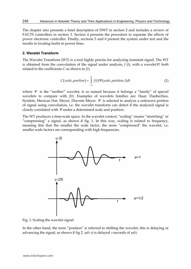
The WT produces a time-scale space. In the wavelet context, “scaling” means “stretching” or “compressing” a signal, as shown if fig. 1. In this way, scaling is related to frequency, meaning this that the smaller the scale factor, the more "compressed" the wavelet, i.e. smaller scale factors are corresponding with high frequencies.

Fig. 1. Scaling the wavelet signal

In the other hand, the term “position” is referred to shifting the wavelet, this is delaying or

advancing the signal, as shown if fig 2. (t-) is delayed seconds of (t).

www.intechopen.com

Discrete Wavelet Transform Application to the Protection of Electrical Power System: A Solution Approach for Detecting and Locating Faults in FACTS Environment

247

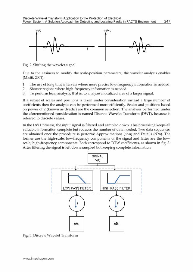
Fig. 2. Shifting the wavelet signal

Due to the easiness to modify the scale-position parameters, the wavelet analysis enables (Misiti, 2001):

1. The use of long time intervals where more precise low-frequency information is needed 2. Shorter regions where high-frequency information is needed. 3. To perform local analysis, that is, to analyze a localized area of a larger signal.

If a subset of scales and positions is taken under consideration instead a large number of coefficients then the analysis can be performed more efficiently. Scales and positions based on power of 2 (known as dyadic) are the common selection. The analysis performed under the aforementioned consideration is named Discrete Wavelet Transform (DWT), because is referred to discrete values.

In the DWT process, the input signal is filtered and sampled down. This processing keeps all valuable information complete but reduces the number of data needed. Two data sequences are obtained once the procedure is perform: Approximations (cAn) and Details (cDn). The former are the high-scale, low-frequency components of the signal and latter are the low-scale, high-frequency components. Both correspond to DTW coefficients, as shown in fig. 3. After filtering the signal is left down sampled but keeping complete information

Fig. 3. Discrete Wavelet Transform

www.intechopen.com


248

cA1 and cD1 are obtained by (2) (Misiti et. al. 2001)

1

1

( ) ( ). ( 2 )

( ) ( ). ( 2 )

dk

dk

cA t f t L k t

cD t f t H k t

(2)

where cA1, is the approximation coefficient of level 1, cD1 is the detail coefficient of level 1. Ld is the low-pass filter and Hd is the high-pass filter. These filters are related to mother

wavelet . In this process, signal f(t) is divided in two sequences, cD1 contains highest frequency components (fs/4 to fs/2 range, where fs equals sampling frequency of f(t)) and cA1 lower frequencies (lower than fs/4). At this stage, cD1 extract elements of f(t) in fs/4 to

fs/2 range that maintains correlation with .

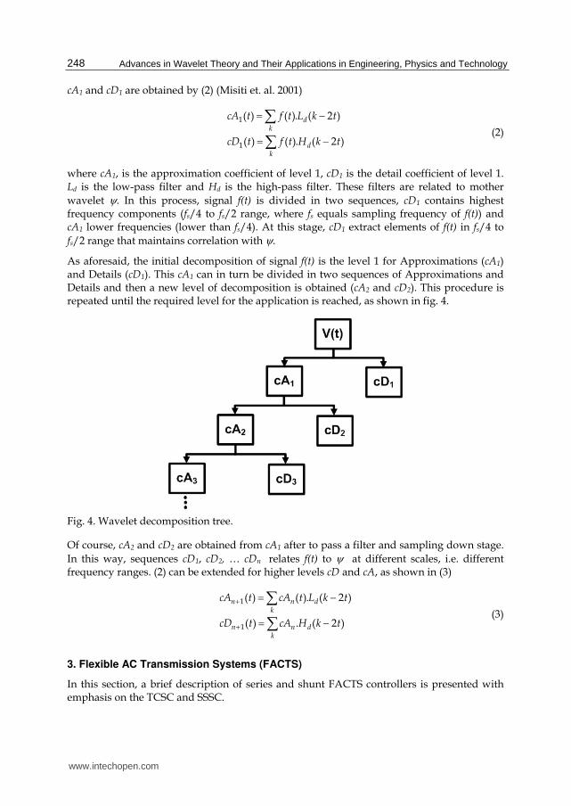
As aforesaid, the initial decomposition of signal f(t) is the level 1 for Approximations (cA1) and Details (cD1). This cA1 can in turn be divided in two sequences of Approximations and Details and then a new level of decomposition is obtained (cA2 and cD2). This procedure is repeated until the required level for the application is reached, as shown in fig. 4.

Fig. 4. Wavelet decomposition tree.

Of course, cA2 and cD2 are obtained from cA1 after to pass a filter and sampling down stage.

In this way, sequences cD1, cD2, … cDn relates f(t) to at different scales, i.e. different frequency ranges. (2) can be extended for higher levels cD and cA, as shown in (3)

1

1

( ) ( ). ( 2 )

( ) . ( 2 )

n n dk

n n dk

cA t cA t L k t

cD t cA H k t

(3)

3. Flexible AC Transmission Systems (FACTS)

In this section, a brief description of series and shunt FACTS controllers is presented with emphasis on the TCSC and SSSC.

www.intechopen.com


249

The FACTS controllers, once installed in the power grid, helps to improve the power transfer capability of long transmission lines and the system performance in general. Some of the benefits of the FACTS controllers on the electric system:

1. Fast voltage regulation, 2. Increased power transfer over long AC lines, 3. Damping of active power oscillations, and 4. Load flow control in meshed systems,

The FACTS controllers are commonly divided in 4 groups (Hingorani&Gyugyi, 2000):

1. Series Controller. These controllers are series connected to a power line. These controllers have an impact on the power flow and voltage profile. Examples of these controllers are the SSSC and TCSC.

2. Shunt Controllers. These controllers are shunt connected and are designed to inject current into the system at the point of connection. An example of these controllers is the Static Synchronous Compensator (STATCOM).

3. Series-shunt controllers. These controllers are a combination of serial and shunt controllers. This combination is capable of injecting current and voltage. An example of these controllers is the Unified Power Flow Controller (UPFC).

4. Series-series controllers. These controllers can be a combination of separate series controllers in a multiline transmission system, or it can be a single controller in a single line. An example of such devices is the Interline Power Flow Controller (IPFC)

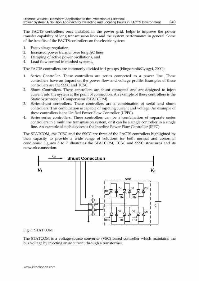
The STATCOM, the TCSC and the SSCC are three of the FACTS controllers highlighted by their capacity to provide a wide range of solutions for both normal and abnormal conditions. Figures 5 to 7 illustrates the STATCOM, TCSC and SSSC structures and its network connection.

Fig. 5. STATCOM

The STATCOM is a voltage-source converter (VSC) based controller which maintains the bus voltage by injecting an ac current through a transformer.

www.intechopen.com


250

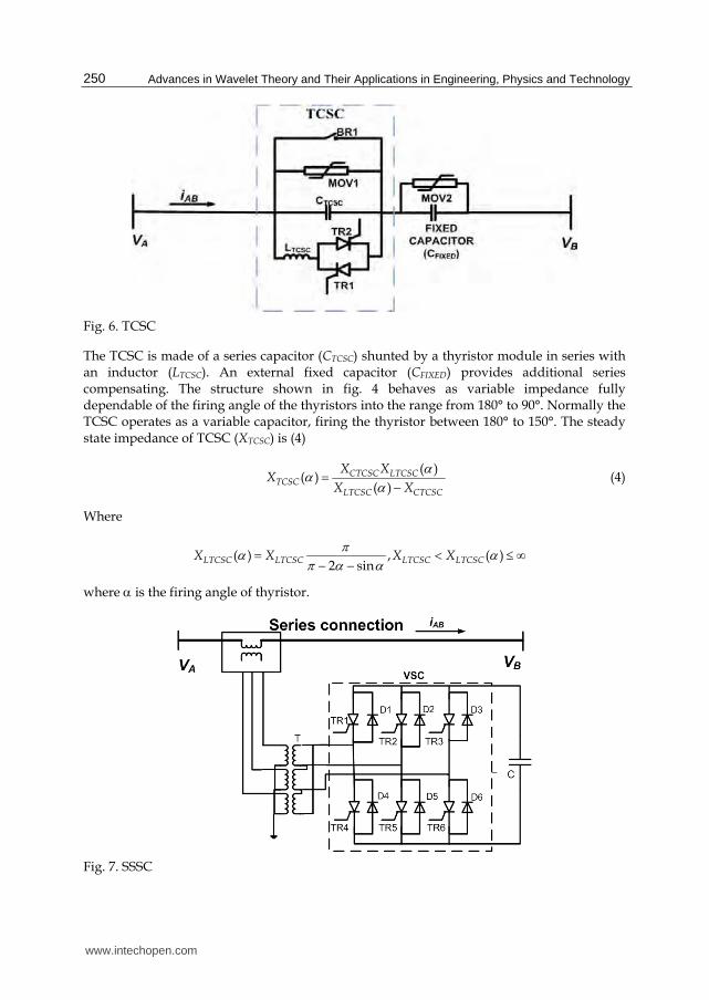
Fig. 6. TCSC

The TCSC is made of a series capacitor (CTCSC) shunted by a thyristor module in series with an inductor (LTCSC). An external fixed capacitor (CFIXED) provides additional series compensating. The structure shown in fig. 4 behaves as variable impedance fully dependable of the firing angle of the thyristors into the range from 180° to 90°. Normally the TCSC operates as a variable capacitor, firing the thyristor between 180° to 150°. The steady state impedance of TCSC (XTCSC) is (4)

( )

( )( )

CTCSC LTCSCTCSC

LTCSC CTCSC

X XX

X X

(4)

Where

( ) , ( )2 sin

LTCSC LTCSC LTCSC LTCSCX X X X

where is the firing angle of thyristor.

Fig. 7. SSSC

www.intechopen.com


251

The SSSC injects a voltage in series with the transmission line in quadrature with the line current. The SSSC increases or decreases the voltage across the line, and thereby, for controlling the transmitted power.

3.1 FACTS effects on conventional protection schemes

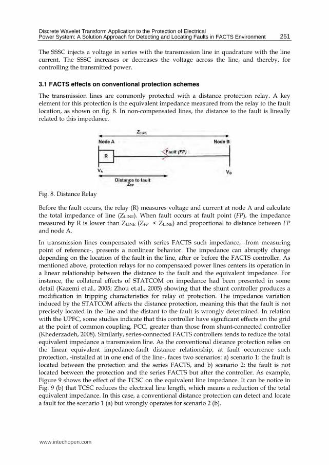
The transmission lines are commonly protected with a distance protection relay. A key element for this protection is the equivalent impedance measured from the relay to the fault location, as shown on fig. 8. In non-compensated lines, the distance to the fault is lineally related to this impedance.

Fig. 8. Distance Relay

Before the fault occurs, the relay (R) measures voltage and current at node A and calculate the total impedance of line (ZLINE). When fault occurs at fault point (FP), the impedance measured by R is lower than ZLINE (ZFP < ZLINE) and proportional to distance between FP and node A.

In transmission lines compensated with series FACTS such impedance, -from measuring point of reference-, presents a nonlinear behavior. The impedance can abruptly change depending on the location of the fault in the line, after or before the FACTS controller. As mentioned above, protection relays for no compensated power lines centers its operation in a linear relationship between the distance to the fault and the equivalent impedance. For instance, the collateral effects of STATCOM on impedance had been presented in some detail (Kazemi et.al., 2005; Zhou et.al., 2005) showing that the shunt controller produces a modification in tripping characteristics for relay of protection. The impedance variation induced by the STATCOM affects the distance protection, meaning this that the fault is not precisely located in the line and the distant to the fault is wrongly determined. In relation with the UPFC, some studies indicate that this controller have significant effects on the grid at the point of common coupling, PCC, greater than those from shunt-connected controller (Khederzadeh, 2008). Similarly, series-connected FACTS controllers tends to reduce the total equivalent impedance a transmission line. As the conventional distance protection relies on the linear equivalent impedance-fault distance relationship, at fault occurrence such protection, -installed at in one end of the line-, faces two scenarios: a) scenario 1: the fault is located between the protection and the series FACTS, and b) scenario 2: the fault is not located between the protection and the series FACTS but after the controller. As example, Figure 9 shows the effect of the TCSC on the equivalent line impedance. It can be notice in Fig. 9 (b) that TCSC reduces the electrical line length, which means a reduction of the total equivalent impedance. In this case, a conventional distance protection can detect and locate a fault for the scenario 1 (a) but wrongly operates for scenario 2 (b).

www.intechopen.com


252

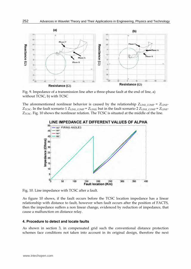
Fig. 9. Impedance of a transmission line after a three-phase fault at the end of line, a) without TCSC, b) with TCSC

The aforementioned nonlinear behavior is caused by the relationship ZLINE_COMP = ZLINE-ZTCSC. In the fault scenario 1 ZLINE_COMP = ZLINE; but in the fault scenario 2 ZLINE_COMP = ZLINE-ZTCSC. Fig. 10 shows the nonlinear relation. The TCSC is situated at the middle of the line.

Fig. 10. Line impedance with TCSC after a fault.

As figure 10 shows, if the fault occurs before the TCSC location impedance has a linear relationship with distance to fault, however when fault occurs after the position of FACTS, then the impedance suffers a non linear change, evidenced by reduction of impedance, that cause a malfunction on distance relay.

4. Procedure to detect and locate faults

As shown in section 3, in compensated grid such the conventional distance protection schemes face conditions not taken into account in its original design, therefore the next

www.intechopen.com


253

generation of protection installed should include algorithms with built-in techniques to deal with the particularities of grids in a FACTS context.

Artificial intelligence and digital signal processing techniques, DSP, have both provided a sort of tools to power systems engineers. In particular the combination of wavelets with artificial intelligence and estimation techniques is an attractive option for analyzing electrical grids in the current context.

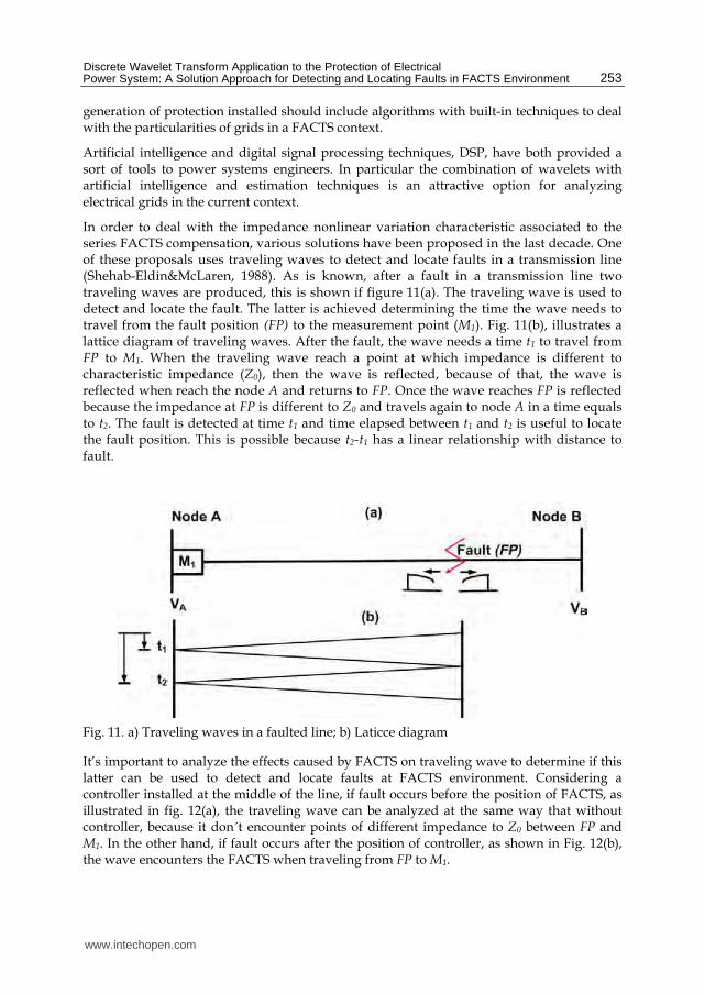
In order to deal with the impedance nonlinear variation characteristic associated to the series FACTS compensation, various solutions have been proposed in the last decade. One of these proposals uses traveling waves to detect and locate faults in a transmission line (Shehab-Eldin&McLaren, 1988). As is known, after a fault in a transmission line two traveling waves are produced, this is shown if figure 11(a). The traveling wave is used to detect and locate the fault. The latter is achieved determining the time the wave needs to travel from the fault position (FP) to the measurement point (M1). Fig. 11(b), illustrates a lattice diagram of traveling waves. After the fault, the wave needs a time t1 to travel from FP to M1. When the traveling wave reach a point at which impedance is different to characteristic impedance (Z0), then the wave is reflected, because of that, the wave is reflected when reach the node A and returns to FP. Once the wave reaches FP is reflected because the impedance at FP is different to Z0 and travels again to node A in a time equals to t2. The fault is detected at time t1 and time elapsed between t1 and t2 is useful to locate the fault position. This is possible because t2-t1 has a linear relationship with distance to fault.

Fig. 11. a) Traveling waves in a faulted line; b) Laticce diagram

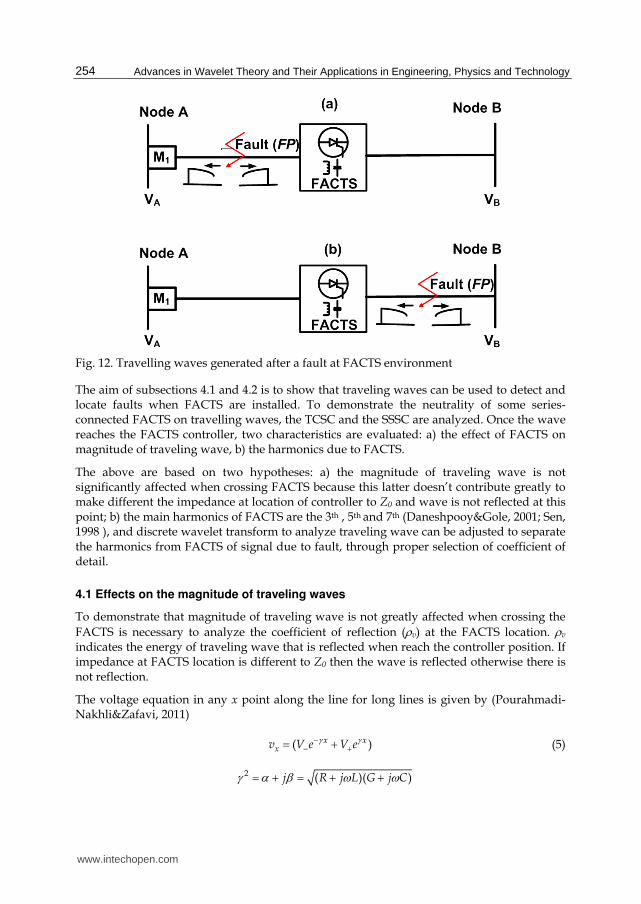
It’s important to analyze the effects caused by FACTS on traveling wave to determine if this latter can be used to detect and locate faults at FACTS environment. Considering a controller installed at the middle of the line, if fault occurs before the position of FACTS, as illustrated in fig. 12(a), the traveling wave can be analyzed at the same way that without controller, because it don´t encounter points of different impedance to Z0 between FP and M1. In the other hand, if fault occurs after the position of controller, as shown in Fig. 12(b), the wave encounters the FACTS when traveling from FP to M1.

www.intechopen.com


254

Fig. 12. Travelling waves generated after a fault at FACTS environment

The aim of subsections 4.1 and 4.2 is to show that traveling waves can be used to detect and locate faults when FACTS are installed. To demonstrate the neutrality of some series-connected FACTS on travelling waves, the TCSC and the SSSC are analyzed. Once the wave reaches the FACTS controller, two characteristics are evaluated: a) the effect of FACTS on magnitude of traveling wave, b) the harmonics due to FACTS.

The above are based on two hypotheses: a) the magnitude of traveling wave is not significantly affected when crossing FACTS because this latter doesn’t contribute greatly to make different the impedance at location of controller to Z0 and wave is not reflected at this point; b) the main harmonics of FACTS are the 3th , 5th and 7th (Daneshpooy&Gole, 2001; Sen, 1998 ), and discrete wavelet transform to analyze traveling wave can be adjusted to separate the harmonics from FACTS of signal due to fault, through proper selection of coefficient of detail.

4.1 Effects on the magnitude of traveling waves

To demonstrate that magnitude of traveling wave is not greatly affected when crossing the

FACTS is necessary to analyze the coefficient of reflection (v) at the FACTS location. v indicates the energy of traveling wave that is reflected when reach the controller position. If impedance at FACTS location is different to Z0 then the wave is reflected otherwise there is not reflection.

The voltage equation in any x point along the line for long lines is given by (Pourahmadi-Nakhli&Zafavi, 2011)

( )x xxv V e V e (5)

2 ( )( )j R j L G j C

www.intechopen.com


255

where is the attenuation constant , is phase constant and is a propagation constant.

V+e+ x represents wave traveling in negative direction and V- e-x represents wave traveling

in positive direction at x point (considering x=0 at node A), as shown in fig. 13.

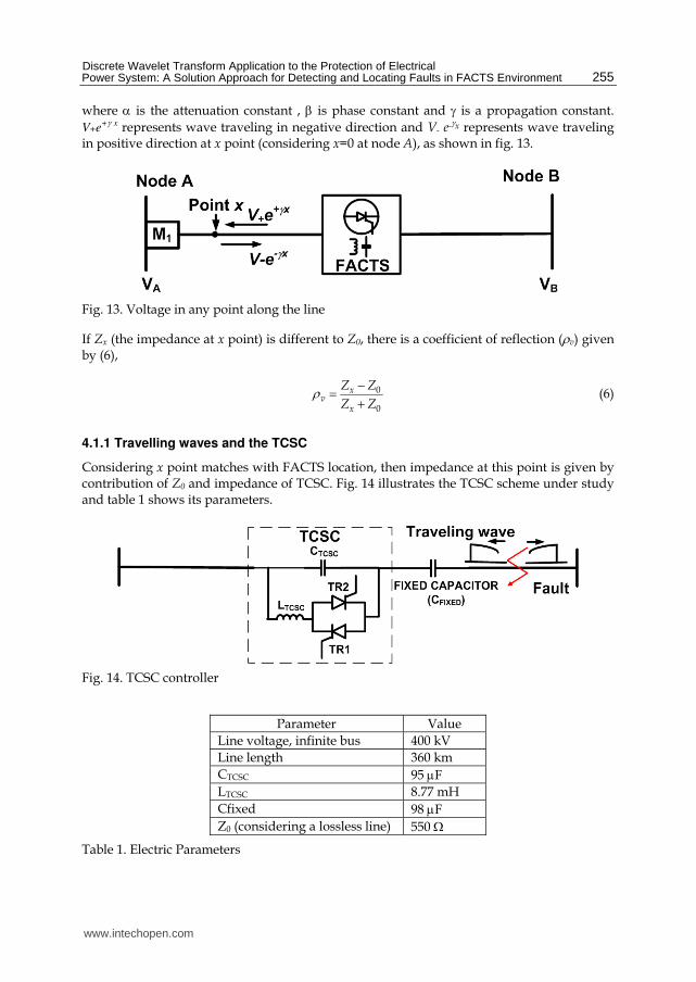
Fig. 13. Voltage in any point along the line

If Zx (the impedance at x point) is different to Z0, there is a coefficient of reflection (v) given by (6),

0

0

xv

x

Z Z

Z Z (6)

4.1.1 Travelling waves and the TCSC

Considering x point matches with FACTS location, then impedance at this point is given by contribution of Z0 and impedance of TCSC. Fig. 14 illustrates the TCSC scheme under study and table 1 shows its parameters.

Fig. 14. TCSC controller

Parameter Value

Line voltage, infinite bus 400 kV

Line length 360 km

CTCSC 95 F

LTCSC 8.77 mH

Cfixed 98 F

Z0 (considering a lossless line) 550

Table 1. Electric Parameters

www.intechopen.com


256

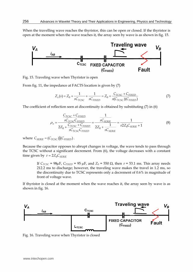
When the travelling wave reaches the thyristor, this can be open or closed. If the thyristor is open at the moment when the wave reaches it, the array seen by wave is as shown in fig. 15.

Fig. 15. Traveling wave when Thyristor is open

From fig. 11, the impedance at FACTS location is given by (7)

0 0

1 1( )

( )( )TCSC FIXED

xTCSC FIXED TCSC FIXED

C CZ s Z Z

sC sC s C C

(7)

The coefficient of reflection seen at discontinuity is obtained by substituting (7) in (6)

0

00

1

1

1 2 122

TCSC FIXED

TCSC FIXED SERIEv

TCSC FIXED SERIE

SERIETCSC FIXED

C C

sC C sC

C C s Z CZZsCsC C

(8)

where ( ) ( )SERIE TCSC FIXEDC C C .

Because the capacitor opposes to abrupt changes in voltage, the wave tends to pass through the TCSC without a significant decrement. From (6), the voltage decreases with a constant

time given by 02 SERIEZ C

If CTCSC = 98F, CFIXED = 95 F, and Z0 = 550 , then = 53.1 ms. This array needs 212.2 ms to discharge; however, the traveling wave makes the travel in 1.2 ms, so the discontinuity due to TCSC represents only a decrement of 0.6% in magnitude of front of voltage wave.

If thyristor is closed at the moment when the wave reaches it, the array seen by wave is as shown in fig. 16.

Fig. 16. Traveling wave when Thyristor is closed

www.intechopen.com


257

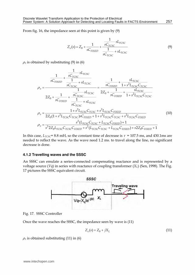
From fig. 16, the impedance seen at this point is given by (9)

0

1

1( )

1

TCSCTCSC

xFIXED

TCSCTCSC

sLsC

Z s ZsC sL

sC

(9)

v is obtained by substituting (9) in (6)

2

0 2

0

2 2

20

1

111

1

1 12

1 12

1

1

2 (1 )

TCSCTCSC

TCSCFIXEDTCSC

FIXEDTCSC TCSC TCSCv

TCSCTCSC

TCSC FIXED TCSC TCSC

FIXEDTCSC

TCSC

TCSC TCSC TCSC FIXEDv

TCSC TCSC FIXED

sLsC

sLsC sLsCsC s L C

sLsL Z

sC sC s L CZ

sC sLsC

s L C s L C

Z s L C sC

2 2

2

3 20 0

1

( ) 1

2 ( ) 2 1

TCSC TCSC TCSC FIXED

TCSC TCSC TCSC FIXEDv

TCSC TCSC FIXED TCSC TCSC TCSC FIXED FIXED

s L C s L C

s L C L C

s Z L C C s L C L C s Z C

(10)

In this case, LTCSC= 8.8 mH, so the constant time of decrease is = 107.5 ms, and 430.1ms are needed to reflect the wave. As the wave need 1.2 ms. to travel along the line, no significant decrease is done.

4.1.2 Travelling waves and the SSSC

An SSSC can emulate a series-connected compensating reactance and is represented by a voltage source (Vq) in series with reactance of coupling transformer (XL) (Sen, 1998). The Fig. 17 pictures the SSSC equivalent circuit.

Fig. 17. SSSC Controller

Once the wave reaches the SSSC, the impedance seen by wave is (11)

0( )x LZ s Z jX (11)

v is obtained substituting (11) in (6)

www.intechopen.com


258

02

Lv

L

jX

jX Z (12)

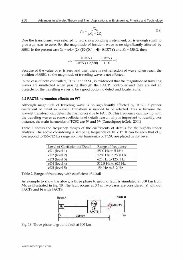
Due the transformer was selected to work as a coupling instrument, XL is enough small to give a v near to zero. So, the magnitude of incident wave is no significantly affected by

SSSC. In the present case XL = wL= (2)(60)(0.1mH)= 0.0377 and Z0 = 550 , then

0.0377 0.03770

0.0377 2(550) 1100v

j j

j

Because of the value of v is zero and then there is not reflection of wave when reach the position of SSSC, so the magnitude of traveling wave is not affected.

In the case of both controllers, TCSC and SSSC, is evidenced that the magnitude of traveling waves are unaffected when passing through the FACTS controller and they are not an obstacle for the travelling waves to be a good option to detect and locate faults.

4.2 FACTS harmonics effects on WT

Although magnitude of traveling wave is no significantly affected by TCSC, a proper coefficient of detail in wavelet transform is needed to be selected. This is because the wavelet transform can detect the harmonics due to FACTS. This frequency can mix up with the traveling waves at some coefficients of details reason why is important to identify. For instance, the main harmonics of TCSC are 3th and 5th (Daneshpooy&Gole, 2001)

Table 2 shows the frequency ranges of the coefficients of details for the signals under analysis. The above considering a sampling frequency of 10 kHz. It can be seen that cD5, correspond to 156-312 Hz range, so main harmonics of TCSC are placed in that level.

Level of Coefficient of Detail Range of frequencycD1 (level 1) 2500 Hz to 5 kHzcD2 (level 2) 1250 Hz to 2500 HzcD3 (level 3) 625 Hz to 1250 HzcD4 (level 4) 312.5 Hz to 625 HzcD5 (level 5) 156 Hz to 312 Hz

Table 2. Range of frequency with coefficient of detail

As example to show the above, a three phase to ground fault is simulated at 300 km from M1, as illustrated in fig. 18. The fault occurs at 0.3 s. Two cases are considered: a) without FACTS and b) with FACTS.

Fig. 18. Three phase to ground fault at 300 km.

www.intechopen.com


259

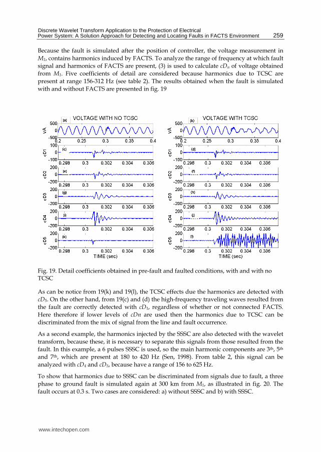
Because the fault is simulated after the position of controller, the voltage measurement in

M1, contains harmonics induced by FACTS. To analyze the range of frequency at which fault

signal and harmonics of FACTS are present, (3) is used to calculate cDn of voltage obtained

from M1. Five coefficients of detail are considered because harmonics due to TCSC are

present at range 156-312 Hz (see table 2). The results obtained when the fault is simulated

with and without FACTS are presented in fig. 19

Fig. 19. Detail coefficients obtained in pre-fault and faulted conditions, with and with no TCSC

As can be notice from 19(k) and 19(l), the TCSC effects due the harmonics are detected with

cD5. On the other hand, from 19(c) and (d) the high-frequency traveling waves resulted from

the fault are correctly detected with cD1, regardless of whether or not connected FACTS.

Here therefore if lower levels of cDn are used then the harmonics due to TCSC can be

discriminated from the mix of signal from the line and fault occurrence.

As a second example, the harmonics injected by the SSSC are also detected with the wavelet

transform, because these, it is necessary to separate this signals from those resulted from the

fault. In this example, a 6 pulses SSSC is used, so the main harmonic components are 3th, 5th

and 7th, which are present at 180 to 420 Hz (Sen, 1998). From table 2, this signal can be

analyzed with cD4 and cD5, because have a range of 156 to 625 Hz.

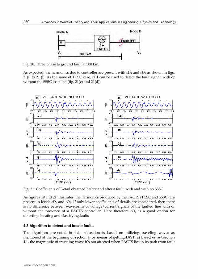
To show that harmonics due to SSSC can be discriminated from signals due to fault, a three

phase to ground fault is simulated again at 300 km from M1, as illustrated in fig. 20. The

fault occurs at 0.3 s. Two cases are considered: a) without SSSC and b) with SSSC.

www.intechopen.com


260

Fig. 20. Three phase to ground fault at 300 km.

As expected, the harmonics due to controller are present with cD4 and cD5 as shown in figs. 21(i) to 21 (l). As the same of TCSC case, cD1 can be used to detect the fault signal, with or without the SSSC installed (fig. 21(c) and 21(d)).

Fig. 21. Coefficients of Detail obtained before and after a fault, with and with no SSSC

As figures 19 and 21 illustrates, the harmonics produced by the FACTS (TCSC and SSSC) are present in levels cD4 and cD5. If only lower coefficients of details are considered, then there is no difference between waveforms of voltage/current signals of the faulted line with or without the presence of a FACTS controller. Here therefore cD1 is a good option for detecting, locating and classifying faults

4.3 Algorithm to detect and locate faults

The algorithm presented in this subsection is based on utilizing traveling waves as mentioned at the beginning of section 4, by means of getting DWT: a) Based on subsection 4.1, the magnitude of traveling wave it’s not affected when FACTS lies in its path from fault

www.intechopen.com


261

position (FP) to measurement point (M1); b) Based on subsection 4.2, harmonics due to FACTS don’t affect the measurement of traveling wave at M1, when cD1 is selected.

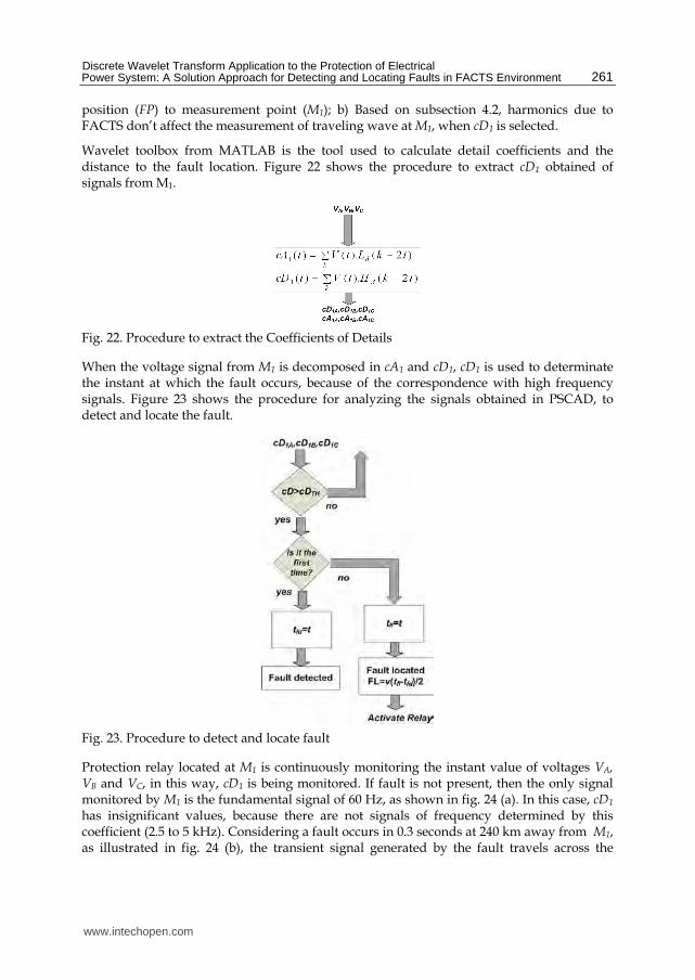
Wavelet toolbox from MATLAB is the tool used to calculate detail coefficients and the distance to the fault location. Figure 22 shows the procedure to extract cD1 obtained of signals from M1.

Fig. 22. Procedure to extract the Coefficients of Details

When the voltage signal from M1 is decomposed in cA1 and cD1, cD1 is used to determinate the instant at which the fault occurs, because of the correspondence with high frequency signals. Figure 23 shows the procedure for analyzing the signals obtained in PSCAD, to detect and locate the fault.

Fig. 23. Procedure to detect and locate fault

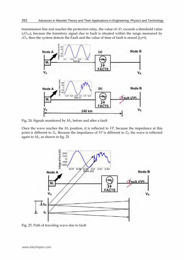
Protection relay located at M1 is continuously monitoring the instant value of voltages VA, VB and VC, in this way, cD1 is being monitored. If fault is not present, then the only signal monitored by M1 is the fundamental signal of 60 Hz, as shown in fig. 24 (a). In this case, cD1 has insignificant values, because there are not signals of frequency determined by this coefficient (2.5 to 5 kHz). Considering a fault occurs in 0.3 seconds at 240 km away from M1, as illustrated in fig. 24 (b), the transient signal generated by the fault travels across the

www.intechopen.com


262

transmission line and reaches the protection relay, the value of cD, exceeds a threshold value (cDTH), because the transitory signal due to fault is situated within the range measured by cD1, then the system detects the Fault and the value of time of fault is stored (tfd=t).

Fig. 24. Signals monitored by M1, before and after a fault

Once the wave reaches the M1 position, it is reflected to FP, because the impedance at this point is different to Z0. Because the impedance of FP is different to Z0, the wave is reflected again to M1, as shown in fig. 25.

Fig. 25. Path of traveling wave due to fault

www.intechopen.com


263

When the traveling wave reaches M1, in a second time, this generates a new peak in cD1 that

uses (13) to locate the distance (FL) at which the fault occurs.

( )

2

fl fdv t tFL

(13)

where v=300,000 (km/s) speed of light, tfl = time of second traveling (s) detection and tfd =

time of first traveling detection (s)

5. System under study

To demonstrate the correct operation of procedure presented in section 4, an electrical grid

was designed in PSCAD. To validate the detection process, several faults are simulated; ten

different types of fault are considered.

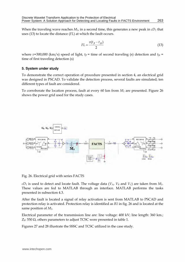
To corroborate the location process, fault at every 60 km from M1 are presented. Figure 26

shows the power grid used for the study cases.

Fig. 26. Electrical grid with series FACTS

cD1 is used to detect and locate fault. The voltage data (VA, VB and VC) are taken from M1.

These values are fed to MATLAB through an interface. MATLAB performs the tasks

presented in subsection 4.3.

After the fault is located a signal of relay activation is sent from MATLAB to PSCAD and

protection relay is activated. Protection relay is identified as B1 in fig. 26 and is located at the

same position of M1.

Electrical parameter of the transmission line are: line voltage: 400 kV; line length: 360 km.;

Z0: 550 , others parameters to adjust TCSC were presented in table 1.

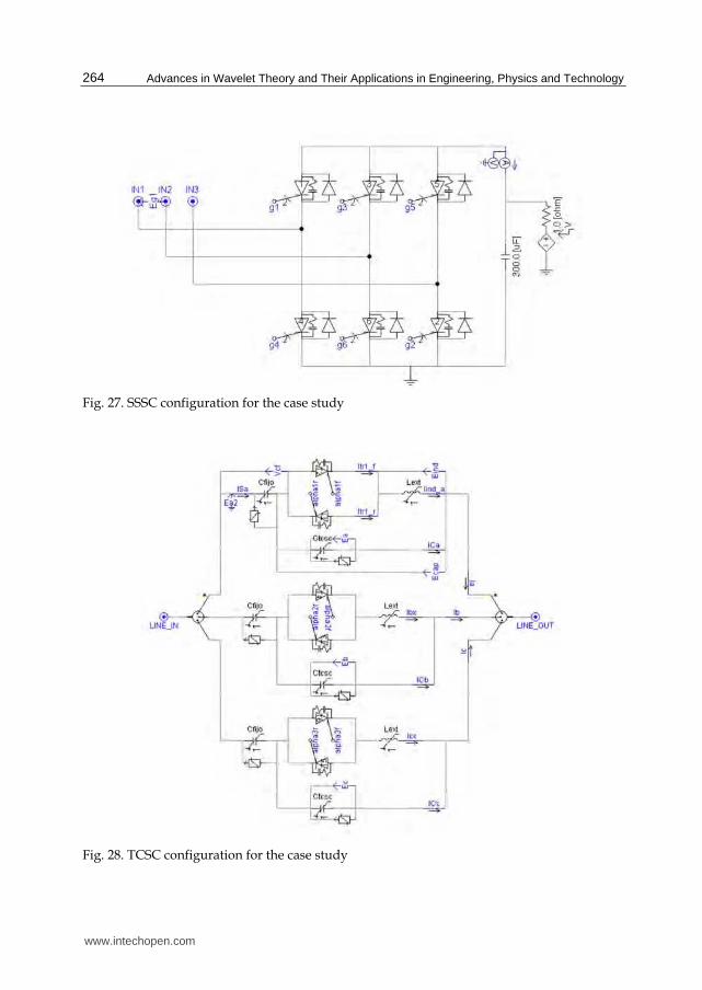
Figures 27 and 28 illustrate the SSSC and TCSC utilized in the case study.

www.intechopen.com


264

Fig. 27. SSSC configuration for the case study

Fig. 28. TCSC configuration for the case study

www.intechopen.com


265

6. Results

As presented in section 4, traveling waves were no significantly affected by presence of FACTS if cD1 is selected. Following the procedure showed in section 4, cD1A, cD1B, cD1C, were employed to detect and locate faults. Ten different types of fault were considered to simulation:

1. AG (Phase A to Ground) 2. BG (Phase B to Ground) 3. CG (Phase C to Ground) 4. ABG (Phases A and B to Ground) 5. ACG (Phases A and C to Ground) 6. BCG (Phases B and C to Ground) 7. ABCG (Three Phase Fault to Ground) 8. AB (Phase A to phase B) 9. AC (Phase A to phase B) 10. BC (Phase A to phase B)

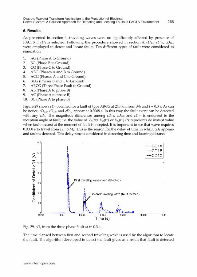
Figure 29 shows cD1 obtained for a fault of type ABCG at 240 km from M1 and t = 0.3 s. As can be notice, cD1A, cD1B, and cD1C appear at 0.3008 s. In this way the fault event can be detected with any cD1. The magnitude differences among cD1A, cD1B, and cD1C is endorsed to the inception angle of fault, i.e. the value of VA(tx), VB(tx) or VC(tx) (tx represents de instant value when fault occurs) at the moment of fault is incepted. It is important to see that wave requires 0.0008 s to travel from FP to M1. This is the reason for the delay of time in which cD1 appears and fault is detected. This delay time is considered in detecting time and locating distance.

Fig. 29. cD1 from the three phase fault at t= 0.3 s.

The time elapsed between first and second traveling wave is used by the algorithm to locate the fault. The algorithm developed to detect the fault gives as a result that fault is detected

www.intechopen.com


266

at 0.3 s and is located at 240 km. These is obtained using (13), in this case, time elapsed between the first and second traveling waves is tfl-tfd = 1.6 ms, so

( ) 300000 / (0.0016 )240

2 2

fl fdv t t km s sFL km

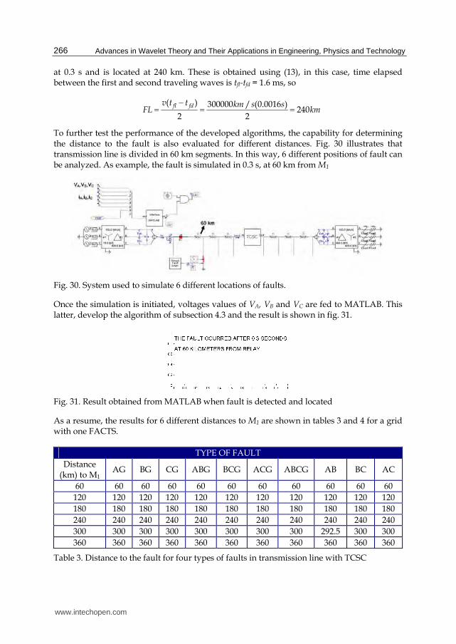
To further test the performance of the developed algorithms, the capability for determining the distance to the fault is also evaluated for different distances. Fig. 30 illustrates that transmission line is divided in 60 km segments. In this way, 6 different positions of fault can be analyzed. As example, the fault is simulated in 0.3 s, at 60 km from M1

Fig. 30. System used to simulate 6 different locations of faults.

Once the simulation is initiated, voltages values of VA, VB and VC are fed to MATLAB. This latter, develop the algorithm of subsection 4.3 and the result is shown in fig. 31.

Fig. 31. Result obtained from MATLAB when fault is detected and located

As a resume, the results for 6 different distances to M1 are shown in tables 3 and 4 for a grid with one FACTS.

TYPE OF FAULT

Distance (km) to M1

AG BG CG ABG BCG ACG ABCG AB BC AC

60 60 60 60 60 60 60 60 60 60 60

120 120 120 120 120 120 120 120 120 120 120

180 180 180 180 180 180 180 180 180 180 180

240 240 240 240 240 240 240 240 240 240 240

300 300 300 300 300 300 300 300 292.5 300 300

360 360 360 360 360 360 360 360 360 360 360

Table 3. Distance to the fault for four types of faults in transmission line with TCSC

www.intechopen.com


267

TYPE OF FAULT

Distance (km) to M1

AG BG CG ABG BCG ACG ABCG AB BC AC

60 60 60 60 60 60 60 60 60 60 60

120 120 120 120 120 120 120 120 120 120 120

180 180 180 180 180 180 180 180 180 180 180

240 240 240 240 240 240 240 240 240 240 240

300 300 300 300 300 300 300 300 292.5 300 300

360 360 360 360 360 360 360 360 360 360 360

Table 4. Distance to the fault for four types of faults in transmission line with SSSC

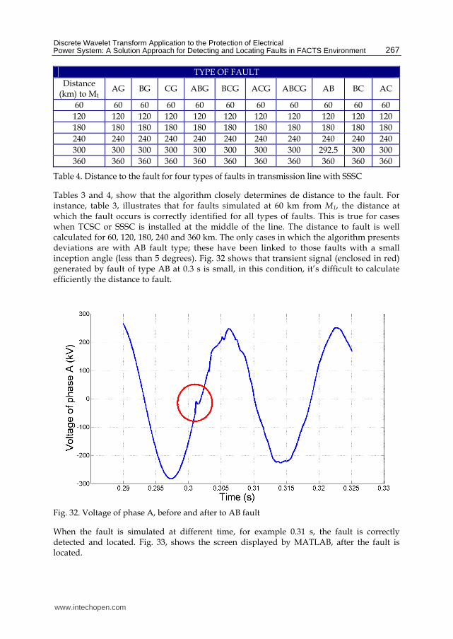
Tables 3 and 4, show that the algorithm closely determines de distance to the fault. For instance, table 3, illustrates that for faults simulated at 60 km from M1, the distance at which the fault occurs is correctly identified for all types of faults. This is true for cases when TCSC or SSSC is installed at the middle of the line. The distance to fault is well calculated for 60, 120, 180, 240 and 360 km. The only cases in which the algorithm presents deviations are with AB fault type; these have been linked to those faults with a small inception angle (less than 5 degrees). Fig. 32 shows that transient signal (enclosed in red) generated by fault of type AB at 0.3 s is small, in this condition, it’s difficult to calculate efficiently the distance to fault.

Fig. 32. Voltage of phase A, before and after to AB fault

When the fault is simulated at different time, for example 0.31 s, the fault is correctly detected and located. Fig. 33, shows the screen displayed by MATLAB, after the fault is located.

www.intechopen.com


268

Fig. 33. Screen displayed after AB fault, in 0.31 s at 300 km from M1

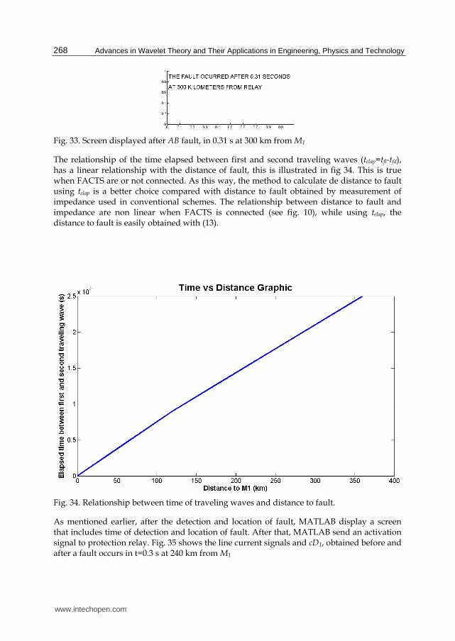
The relationship of the time elapsed between first and second traveling waves (telap=tfl-tfd), has a linear relationship with the distance of fault, this is illustrated in fig 34. This is true when FACTS are or not connected. As this way, the method to calculate de distance to fault using telap is a better choice compared with distance to fault obtained by measurement of impedance used in conventional schemes. The relationship between distance to fault and impedance are non linear when FACTS is connected (see fig. 10), while using telap, the distance to fault is easily obtained with (13).

Fig. 34. Relationship between time of traveling waves and distance to fault.

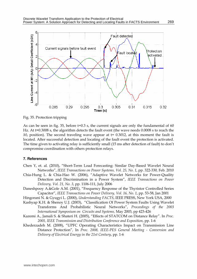
As mentioned earlier, after the detection and location of fault, MATLAB display a screen that includes time of detection and location of fault. After that, MATLAB send an activation signal to protection relay. Fig. 35 shows the line current signals and cD1, obtained before and after a fault occurs in t=0.3 s at 240 km from M1

www.intechopen.com


269

Fig. 35. Protection tripping

As can be seen in fig. 35, before t=0.3 s, the current signals are only the fundamental of 60 Hz. At t=0.3008 s, the algorithm detects the fault event (the wave needs 0.0008 s to reach the M1 position). The second traveling wave appear at t= 0.3012, at this moment the fault is located. After successful detection and locating of the fault event the protection is activated. The time given to activating relay is sufficiently small (15 ms after detection of fault) to don’t compromise coordination with others protection relays.

7. References

Chen Y, et. al. (2010), “Short-Term Load Forecasting: Similar Day-Based Wavelet Neural Networks”, IEEE Transactions on Power Systems, Vol. 25, No. 1, pp. 322-330, Feb. 2010

Chia-Hung L. & Chia-Hao W. (2006), “Adaptive Wavelet Networks for Power-Quality Detection and Discrimination in a Power System”, IEEE Transactions on Power Delivery, Vol. 21, No. 3, pp. 1106-111, July 2006

Daneshpooy A.&Gole A.M. (2001), “Frequency Response of the Thyristor Controlled Series Capacitor”, IEEE Transactions on Power Delivery, Vol. 16, No. 1, pp. 53-58, Jan 2001

Hingorani N. & Gyugyi L. (2000), Understanding FACTS, IEEE PRESS, New York USA, 2000 Kashyap K.H. & Shenoy U.J. (2003), “Classification Of Power System Faults Using Wavelet

Transforms And Probabilistic Neural Networks”, Proceedings of the 2003 International Symposium on Circuits and Systems, May 2003, pp 423-426

Kazemi A., Jamali S. & Shateri H. (2005), “Effects of STATCOM on Distance Relay”. In Proc. 2005, IEEE Transmission and Distribution Conference and Exposition, pp. 1-6

Khederzadeh M. (2008), “UPFC Operating Characteristics Impact on Transmission Line Distance Protection”, In Proc. 2008, IEEE-PES General Meeting - Conversion and Delivery of Electrical Energy in the 21st Century, pp. 1-6

www.intechopen.com


270

Misiti M., Oppenheim & Poggi J. M. (2001), “Wavelet Toolbox Users Guide”, The Math Work, Inc., 2001

Ning J. & Gao W. (2009), “A wavelet-based method to extract frequency feature for power system fault/event analysis”, Power & Energy Society General Meeting, IEEE, Calgary, AB, Oct. 2009.

Pourahmadi-Nakhli M. & Safavi A. (2011), “Path Characteristic Frequency-Based Fault Locating in Radial Distribution Systems Using Wavelets and Neural Networks”, IEEE Trans. on Power Delivery, vol. 26, pp. 772-781, Apr. 2011.

Sen K.K. (1998), “SSSC - Static Synchronous Series Compensator: Theory, Modeling, and Applications”, IEEE Trans. on Power Delivery, vol. 13, pp. 241-246, Jan. 1998

Shehab-Eldin E.H. & McLaren P.G. (1988), “Travelling wave distance protection - problem areas and solutions”, IEEE Trans. on Power Delivery, Vol. 3, No. 3, pp. 894-902, Jul. 1988

Tse N.C.F (2006), “Practical application of wavelet to power quality analysis”, Power Engineering Society General Meeting, IEEE, Montreal, Que, Oct. 2006.

Zhou X.Y, Wang H.F., Aggarwal R.K. & Beaumont P. (2005), “The Impact of STATCOM on Distance Relay”, In Proc. 2005, Power Systems Computation Conference, pp. 1-7

www.intechopen.com

Advances in Wavelet Theory and Their Applications inEngineering, Physics and TechnologyEdited by Dr. Dumitru Baleanu

ISBN 978-953-51-0494-0Hard cover, 634 pagesPublisher InTechPublished online 04, April, 2012Published in print edition April, 2012

InTech EuropeUniversity Campus STeP Ri Slavka Krautzeka 83/A 51000 Rijeka, Croatia Phone: +385 (51) 770 447 Fax: +385 (51) 686 166www.intechopen.com

InTech ChinaUnit 405, Office Block, Hotel Equatorial Shanghai No.65, Yan An Road (West), Shanghai, 200040, China

Phone: +86-21-62489820 Fax: +86-21-62489821

The use of the wavelet transform to analyze the behaviour of the complex systems from various fields startedto be widely recognized and applied successfully during the last few decades. In this book some advances inwavelet theory and their applications in engineering, physics and technology are presented. The applicationswere carefully selected and grouped in five main sections - Signal Processing, Electrical Systems, FaultDiagnosis and Monitoring, Image Processing and Applications in Engineering. One of the key features of thisbook is that the wavelet concepts have been described from a point of view that is familiar to researchers fromvarious branches of science and engineering. The content of the book is accessible to a large number ofreaders.

How to referenceIn order to correctly reference this scholarly work, feel free to copy and paste the following:

Enrique Reyes-Archundia, Edgar L. Moreno-Goytia, Jose Antonio Gutierrez-Gnecchi and Francisco Rivas-Davalos (2012). Discrete Wavelet Transform Application to the Protection of Electrical Power System: ASolution Approach for Detecting and Locating Faults in FACTS Environment, Advances in Wavelet Theory andTheir Applications in Engineering, Physics and Technology, Dr. Dumitru Baleanu (Ed.), ISBN: 978-953-51-0494-0, InTech, Available from: http://www.intechopen.com/books/advances-in-wavelet-theory-and-their-applications-in-engineering-physics-and-technology/discrete-wavelet-transform-application-to-the-protection-of-electrical-power-system-a-solution-appro

Discrete Wavelet Transform Application to the Protection ...cdn.intechopen.com/pdfs/34958/InTech-Discrete_wavelet_transform... · 12 Discrete Wavelet Transform Application to the

Documents