Discrete random variables - … · Discrete random variables Bernoulli’s random variable ∼ ( ) ∙it is the simplest discrete random variable, it models an experiment in

Special Mathematics

Discrete random variables

April 2018

ii

” Expose yourself to as much randomness as possible. ”

Ben Casnocha

6Discrete random variables

Texas Holdem Poker:

In Hold’em Poker players make the best hand they can combining the twocards in their hand with the 5 cards (community cards) eventually turned upon the table. The deck has 52 and there are 13 of each suit: ♣ ♦ ♥ ♠

Open problem: Until he finally won a WSOP event in 2008, Erick Lind-gren was often called one of the greatest players never to have won a WSOPtournament. Before his win, he played in many WSOP events and finished in

1

the top 10 eight times. Suppose you play in one tournament per week. Forsimplicity, assume that each tournament’s results are independent of the oth-ers and that you have the same probability p of winning each tournament. If𝑝 = 0.01, then what is the expected amount of time before you win your firsttournament?

Open problem: During Episode 2 of Season 5 of High Stakes Poker, DoyleBrunson was dealt pocket kings twice and pocket jacks once, all within abouthalf an hour. Suppose we consider a high pocket pair to mean 10-10, J-J, Q-Q,K-K, or A-A. Let 𝑋 be the number of hands you play until you are dealt ahigh pocket pair for the third time. What is the expected number of hands ?

Open problem: Many casinos award prizes for rare events called jackpothands. These jackpot hands are defined differently by different casinos. Supposein a certain casino jackpot hands are defined so that they tend to occur aboutonce every 50, 000 hands on average. If the casino deals about 10, 000 handsper day, what are the expected value and standard deviation of the number ofjackpot hands dealt in a 7-day period?

Open problem: On the last hand of the 1998 WSOP Main Event, with theboard 8 ♣ 9 ♦ 9 ♥ 8 ♥ 8 ♠, Scotty Nguyen went all-in. While his opponent,Kevin McBride, was thinking, Scotty said, “You call, it’s gonna be all over,baby.” McBride said, “I call. I play the board.” It turned out that Scotty hadJ ♦ 9 ♣ and won the hand. Assuming you never fold in the next 100 hands,what would be the expected value of X = the number of times in these 100hands that you would play the board after all five board cards are dealt ?

2

Discrete random variables

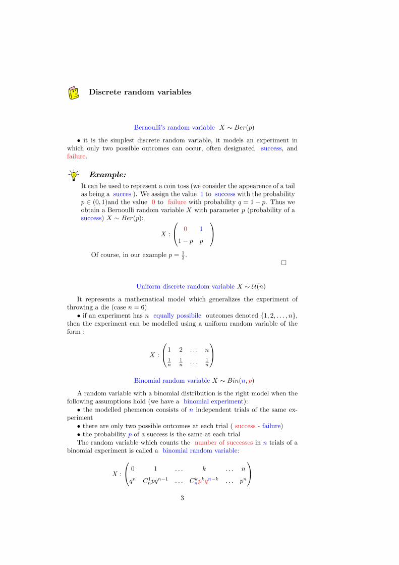
Bernoulli’s random variable 𝑋 ∼ 𝐵𝑒𝑟(𝑝)

∙ it is the simplest discrete random variable, it models an experiment inwhich only two possible outcomes can occur, often designated success, andfailure.

It can be used to represent a coin toss (we consider the appearence of a tailas being a succes ). We assign the value 1 to success with the probability𝑝 ∈ (0, 1)and the value 0 to failure with probability 𝑞 = 1 − 𝑝. Thus weobtain a Bernoulli random variable 𝑋 with parameter 𝑝 (probability of asuccess) 𝑋 ∼ 𝐵𝑒𝑟(𝑝):

𝑋 :

⎛⎝ 0 1

1 − 𝑝 𝑝

⎞⎠Of course, in our example 𝑝 = 1

2 .�

Example:

Uniform discrete random variable 𝑋 ∼ 𝒰(𝑛)

It represents a mathematical model which generalizes the experiment ofthrowing a die (case 𝑛 = 6)

∙ if an experiment has 𝑛 equally possibile outcomes denoted {1, 2, . . . , 𝑛},then the experiment can be modelled using a uniform random variable of theform :

𝑋 :

⎛⎝1 2 . . . 𝑛

1𝑛

1𝑛 . . . 1

𝑛

⎞⎠Binomial random variable 𝑋 ∼ 𝐵𝑖𝑛(𝑛, 𝑝)

A random variable with a binomial distribution is the right model when thefollowing assumptions hold (we have a binomial experiment):

∙ the modelled phemenon consists of 𝑛 independent trials of the same ex-periment

∙ there are only two possible outcomes at each trial ( success - failure)∙ the probability 𝑝 of a success is the same at each trialThe random variable which counts the number of successes in 𝑛 trials of a

binomial experiment is called a binomial random variable:

𝑋 :

⎛⎝ 0 1 . . . 𝑘 . . . 𝑛

𝑞𝑛 𝐶1𝑛𝑝𝑞

𝑛−1 . . . 𝐶𝑘𝑛𝑝

𝑘𝑞𝑛−𝑘 . . . 𝑝𝑛

⎞⎠3

where 𝑝 and 𝑞 = 1 − 𝑝 are the probabilities of a success, respectively failure ateach independent trial.

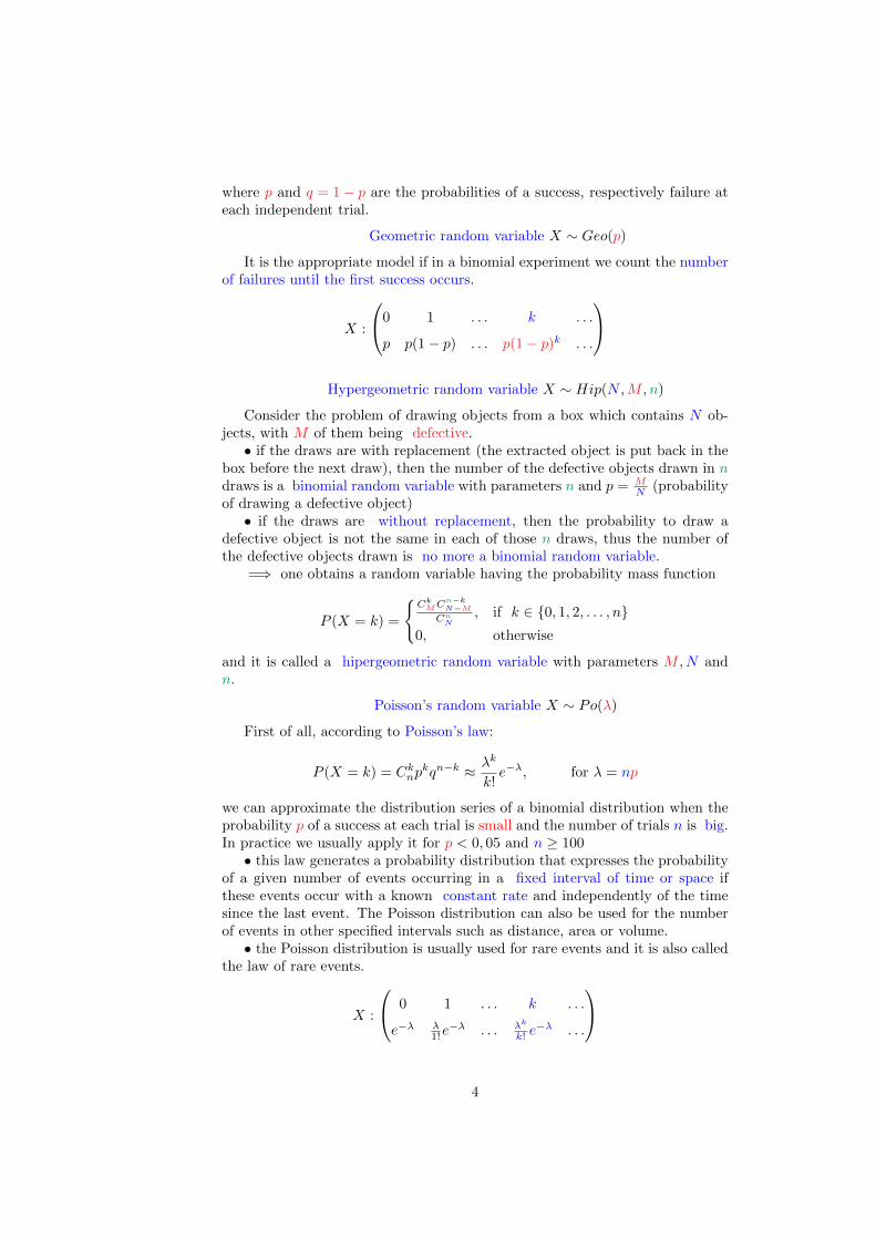
Geometric random variable 𝑋 ∼ 𝐺𝑒𝑜(𝑝)

It is the appropriate model if in a binomial experiment we count the numberof failures until the first success occurs.

𝑋 :

⎛⎝0 1 . . . 𝑘 . . .

𝑝 𝑝(1 − 𝑝) . . . 𝑝(1 − 𝑝)𝑘 . . .

⎞⎠Hypergeometric random variable 𝑋 ∼ 𝐻𝑖𝑝(𝑁,𝑀,𝑛)

Consider the problem of drawing objects from a box which contains 𝑁 ob-jects, with 𝑀 of them being defective.

∙ if the draws are with replacement (the extracted object is put back in thebox before the next draw), then the number of the defective objects drawn in 𝑛draws is a binomial random variable with parameters 𝑛 and 𝑝 = 𝑀

𝑁 (probabilityof drawing a defective object)

∙ if the draws are without replacement, then the probability to draw adefective object is not the same in each of those 𝑛 draws, thus the number ofthe defective objects drawn is no more a binomial random variable.

=⇒ one obtains a random variable having the probability mass function

𝑃 (𝑋 = 𝑘) =

{︃𝐶𝑘

𝑀𝐶𝑛−𝑘𝑁−𝑀

𝐶𝑛𝑁

, if 𝑘 ∈ {0, 1, 2, . . . , 𝑛}0, otherwise

and it is called a hipergeometric random variable with parameters 𝑀,𝑁 and𝑛.

Poisson’s random variable 𝑋 ∼ 𝑃𝑜(𝜆)

First of all, according to Poisson’s law:

𝑃 (𝑋 = 𝑘) = 𝐶𝑘𝑛𝑝

𝑘𝑞𝑛−𝑘 ≈ 𝜆𝑘

𝑘!𝑒−𝜆, for 𝜆 = 𝑛𝑝

we can approximate the distribution series of a binomial distribution when theprobability 𝑝 of a success at each trial is small and the number of trials 𝑛 is big.In practice we usually apply it for 𝑝 < 0, 05 and 𝑛 ≥ 100

∙ this law generates a probability distribution that expresses the probabilityof a given number of events occurring in a fixed interval of time or space ifthese events occur with a known constant rate and independently of the timesince the last event. The Poisson distribution can also be used for the numberof events in other specified intervals such as distance, area or volume.

∙ the Poisson distribution is usually used for rare events and it is also calledthe law of rare events.

𝑋 :

⎛⎝ 0 1 . . . 𝑘 . . .

𝑒−𝜆 𝜆1!𝑒

−𝜆 . . . 𝜆𝑘

𝑘! 𝑒−𝜆 . . .

⎞⎠

4

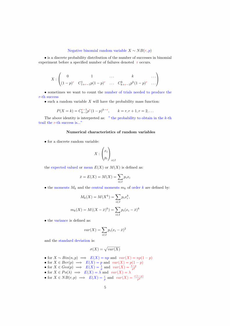
Negative binomial random variable 𝑋 ∼ 𝑁𝐵(𝑟, 𝑝)

∙ is a discrete probability distribution of the number of successes in binomialexperiment before a specified number of failures denoted r occurs.

𝑋 :

⎛⎝ 0 1 . . . 𝑘 . . .

(1 − 𝑝)𝑟 𝐶11+𝑟−1𝑝(1 − 𝑝)𝑟 . . . 𝐶𝑘

𝑘+𝑟−1𝑝𝑘(1 − 𝑝)𝑟 . . .

⎞⎠∙ sometimes we want to count the number of trials needed to produce the

𝑟-th success∙ such a random variable 𝑋 will have the probability mass function:

𝑃 (𝑋 = 𝑘) = 𝐶𝑟−1𝑘−1𝑝

𝑟(1 − 𝑝)𝑘−𝑟, 𝑘 = 𝑟, 𝑟 + 1, 𝑟 = 2, . . .

The above identity is interpreted as: ” the probability to obtain in the 𝑘-thtrail the 𝑟-th success is...”

Numerical characteristics of random variables

∙ for a discrete random variable:

𝑋 :

⎛⎝𝑥𝑖

𝑝𝑖

⎞⎠𝑖∈𝐼

the expected valued or mean 𝐸(𝑋) or 𝑀(𝑋) is defined as:

�̄� = 𝐸(𝑋) = 𝑀(𝑋) =∑︁𝑖∈𝐼

𝑝𝑖𝑥𝑖

∙ the moments 𝑀𝑘 and the central moments 𝑚𝑘 of order 𝑘 are defined by:

𝑀𝑘(𝑋) = 𝑀(𝑋𝑘) =∑︁𝑖∈𝐼

𝑝𝑖𝑥𝑘𝑖 ,

𝑚𝑘(𝑋) = 𝑀((𝑋 − �̄�)𝑘) =∑︁𝑖∈𝐼

𝑝𝑖(𝑥𝑖 − �̄�)𝑘

∙ the variance is defined as:

𝑣𝑎𝑟(𝑋) =∑︁𝑖∈𝐼

𝑝𝑖(𝑥𝑖 − �̄�)2

and the standard deviation is:

𝜎(𝑋) =√︀

𝑣𝑎𝑟(𝑋)

∙ for 𝑋 ∼ 𝐵𝑖𝑛(𝑛, 𝑝) =⇒ 𝐸(𝑋) = 𝑛𝑝 and 𝑣𝑎𝑟(𝑋) = 𝑛𝑝(1 − 𝑝)∙ for 𝑋 ∈ 𝐵𝑒𝑟(𝑝) =⇒ 𝐸(𝑋) = 𝑝 and 𝑣𝑎𝑟(𝑋) = 𝑝(1 − 𝑝)∙ for 𝑋 ∈ 𝐺𝑒𝑜(𝑝) =⇒ 𝐸(𝑋) = 1

𝑝 and 𝑣𝑎𝑟(𝑋) = 1−𝑝𝑝2

∙ for 𝑋 ∈ 𝑃𝑜(𝜆) =⇒ 𝐸(𝑋) = 𝜆 and 𝑣𝑎𝑟(𝑋) = 𝜆

∙ for 𝑋 ∈ 𝑁𝐵(𝑟, 𝑝) =⇒ 𝐸(𝑋) = 𝑟𝑝 and 𝑣𝑎𝑟(𝑋) = 𝑟(1−𝑝)

𝑝2

5

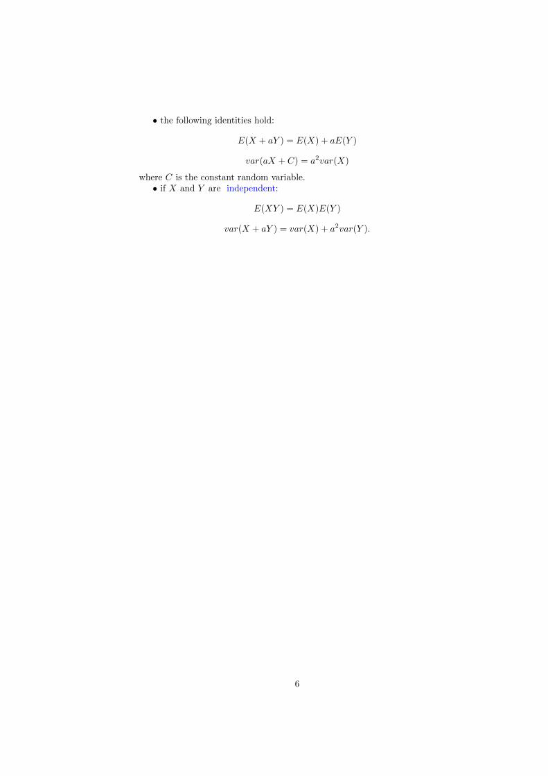
∙ the following identities hold:

𝐸(𝑋 + 𝑎𝑌 ) = 𝐸(𝑋) + 𝑎𝐸(𝑌 )

𝑣𝑎𝑟(𝑎𝑋 + 𝐶) = 𝑎2𝑣𝑎𝑟(𝑋)

where 𝐶 is the constant random variable.∙ if 𝑋 and 𝑌 are independent:

𝐸(𝑋𝑌 ) = 𝐸(𝑋)𝐸(𝑌 )

𝑣𝑎𝑟(𝑋 + 𝑎𝑌 ) = 𝑣𝑎𝑟(𝑋) + 𝑎2𝑣𝑎𝑟(𝑌 ).

6

Solved problems

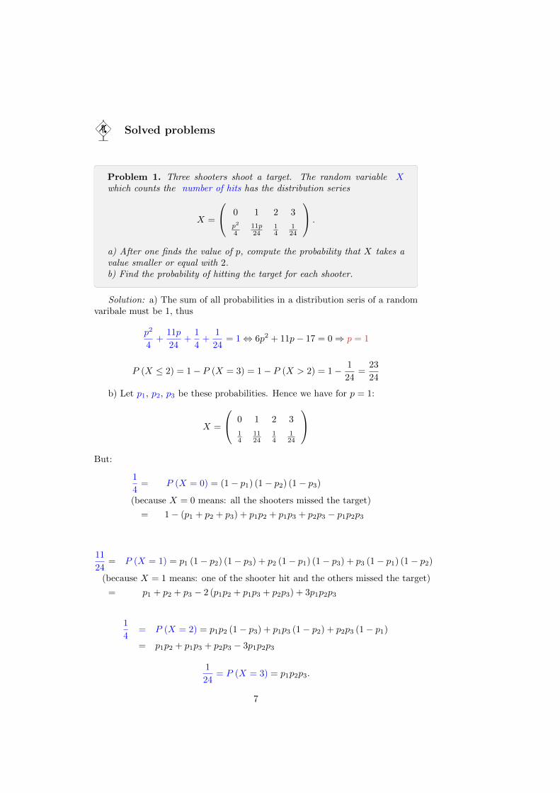
Problem 1. Three shooters shoot a target. The random variable 𝑋which counts the number of hits has the distribution series

𝑋 =

⎛⎝ 0 1 2 3

𝑝2

411𝑝24

14

124

⎞⎠ .

a) After one finds the value of 𝑝, compute the probability that 𝑋 takes avalue smaller or equal with 2.b) Find the probability of hitting the target for each shooter.

Solution: a) The sum of all probabilities in a distribution seris of a randomvaribale must be 1, thus

𝑝2

4+

11𝑝

24+

1

4+

1

24= 1 ⇔ 6𝑝2 + 11𝑝− 17 = 0 ⇒ 𝑝 = 1

𝑃 (𝑋 ≤ 2) = 1 − 𝑃 (𝑋 = 3) = 1 − 𝑃 (𝑋 > 2) = 1 − 1

24=

23

24

b) Let 𝑝1, 𝑝2, 𝑝3 be these probabilities. Hence we have for 𝑝 = 1:

𝑋 =

⎛⎝ 0 1 2 3

14

1124

14

124

⎞⎠But:

1

4= 𝑃 (𝑋 = 0) = (1 − 𝑝1) (1 − 𝑝2) (1 − 𝑝3)

(because 𝑋 = 0 means: all the shooters missed the target)

= 1 − (𝑝1 + 𝑝2 + 𝑝3) + 𝑝1𝑝2 + 𝑝1𝑝3 + 𝑝2𝑝3 − 𝑝1𝑝2𝑝3

11

24= 𝑃 (𝑋 = 1) = 𝑝1 (1 − 𝑝2) (1 − 𝑝3) + 𝑝2 (1 − 𝑝1) (1 − 𝑝3) + 𝑝3 (1 − 𝑝1) (1 − 𝑝2)

(because 𝑋 = 1 means: one of the shooter hit and the others missed the target)

= 𝑝1 + 𝑝2 + 𝑝3 − 2 (𝑝1𝑝2 + 𝑝1𝑝3 + 𝑝2𝑝3) + 3𝑝1𝑝2𝑝3

1

4= 𝑃 (𝑋 = 2) = 𝑝1𝑝2 (1 − 𝑝3) + 𝑝1𝑝3 (1 − 𝑝2) + 𝑝2𝑝3 (1 − 𝑝1)

= 𝑝1𝑝2 + 𝑝1𝑝3 + 𝑝2𝑝3 − 3𝑝1𝑝2𝑝3

1

24= 𝑃 (𝑋 = 3) = 𝑝1𝑝2𝑝3.

7

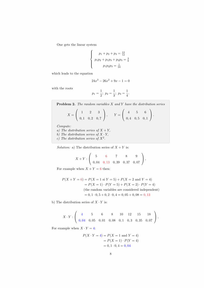
One gets the linear system⎧⎪⎪⎪⎨⎪⎪⎪⎩𝑝1 + 𝑝2 + 𝑝3 = 13

12

𝑝1𝑝2 + 𝑝1𝑝3 + 𝑝2𝑝3 = 38

𝑝1𝑝2𝑝3 = 124

which leads to the equation

24𝑥3 − 26𝑥2 + 9𝑥− 1 = 0

with the roots

𝑝1 =1

2; 𝑝2 =

1

3; 𝑝3 =

1

4.

Problem 2. The random variables 𝑋 and 𝑌 have the distribution series

𝑋 =

⎛⎝ 1 2 3

0, 1 0, 2 0, 7

⎞⎠ , 𝑌 =

⎛⎝ 4 5 6

0, 4 0, 5 0, 1

⎞⎠ .

Compute:a) The distribution series of 𝑋 + 𝑌,b) The distribution series of 𝑋 · 𝑌,c) The distribution series of 𝑋2.

Solution: a) The distribution series of 𝑋 + 𝑌 is:

𝑋 + 𝑌 :

⎛⎝ 5 6 7 8 9

0, 04 0, 13 0, 39 0, 37 0, 07

⎞⎠ ,

For example when 𝑋 + 𝑌 = 6 then:

𝑃 (𝑋 + 𝑌 = 6) = 𝑃 (𝑋 = 1 si 𝑌 = 5) + 𝑃 (𝑋 = 2 and 𝑌 = 4)

= 𝑃 (𝑋 = 1) · 𝑃 (𝑌 = 5) + 𝑃 (𝑋 = 2) · 𝑃 (𝑌 = 4)

(the random variables are considered independent)

= 0, 1 · 0, 5 + 0, 2 · 0, 4 = 0, 05 + 0, 08 = 0, 13

b) The distribution series of 𝑋 · 𝑌 is:

𝑋 · 𝑌 :

⎛⎝ 4 5 6 8 10 12 15 18

0, 04 0, 05 0, 01 0, 08 0, 1 0, 3 0, 35 0, 07

⎞⎠ ,

For example when 𝑋 · 𝑌 = 4:

𝑃 (𝑋 · 𝑌 = 4) = 𝑃 (𝑋 = 1 and 𝑌 = 4)

= 𝑃 (𝑋 = 1) · 𝑃 (𝑌 = 4)

= 0, 1 · 0, 4 = 0, 04

8

again using the independence of 𝑋 and 𝑌 we were able to compute straightfor-ward 𝑃 (𝑋 = 1 and 𝑌 = 4) = 𝑃 (𝑋 = 1) · 𝑃 (𝑌 = 4).

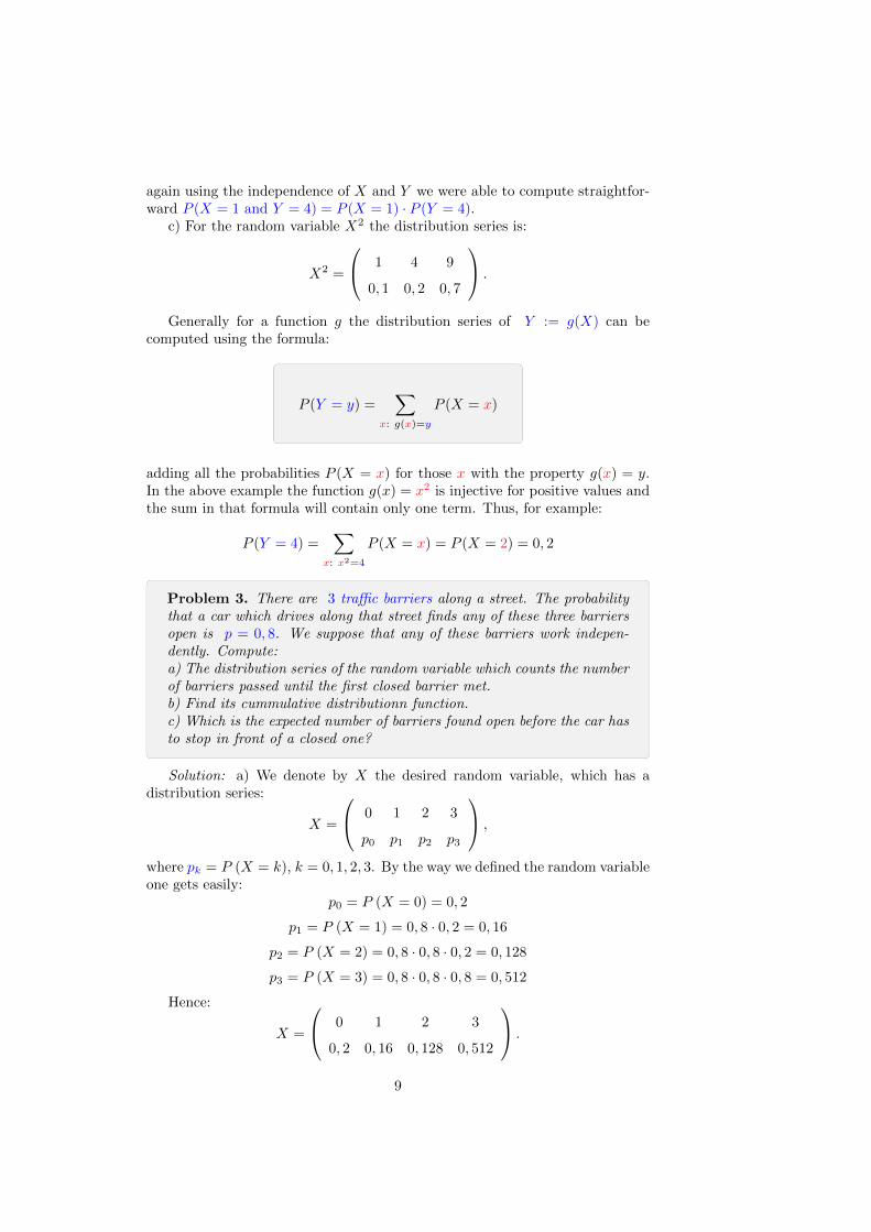
c) For the random variable 𝑋2 the distribution series is:

𝑋2 =

⎛⎝ 1 4 9

0, 1 0, 2 0, 7

⎞⎠ .

Generally for a function 𝑔 the distribution series of 𝑌 := 𝑔(𝑋) can becomputed using the formula:

𝑃 (𝑌 = 𝑦) =∑︁

𝑥: 𝑔(𝑥)=𝑦

𝑃 (𝑋 = 𝑥)

adding all the probabilities 𝑃 (𝑋 = 𝑥) for those 𝑥 with the property 𝑔(𝑥) = 𝑦.In the above example the function 𝑔(𝑥) = 𝑥2 is injective for positive values andthe sum in that formula will contain only one term. Thus, for example:

𝑃 (𝑌 = 4) =∑︁

𝑥: 𝑥2=4

𝑃 (𝑋 = 𝑥) = 𝑃 (𝑋 = 2) = 0, 2

Problem 3. There are 3 traffic barriers along a street. The probabilitythat a car which drives along that street finds any of these three barriersopen is 𝑝 = 0, 8. We suppose that any of these barriers work indepen-dently. Compute:a) The distribution series of the random variable which counts the numberof barriers passed until the first closed barrier met.b) Find its cummulative distributionn function.c) Which is the expected number of barriers found open before the car hasto stop in front of a closed one?

Solution: a) We denote by 𝑋 the desired random variable, which has adistribution series:

𝑋 =

⎛⎝ 0 1 2 3

𝑝0 𝑝1 𝑝2 𝑝3

⎞⎠ ,

where 𝑝𝑘 = 𝑃 (𝑋 = 𝑘), 𝑘 = 0, 1, 2, 3. By the way we defined the random variableone gets easily:

𝑝0 = 𝑃 (𝑋 = 0) = 0, 2

𝑝1 = 𝑃 (𝑋 = 1) = 0, 8 · 0, 2 = 0, 16

𝑝2 = 𝑃 (𝑋 = 2) = 0, 8 · 0, 8 · 0, 2 = 0, 128

𝑝3 = 𝑃 (𝑋 = 3) = 0, 8 · 0, 8 · 0, 8 = 0, 512

Hence:

𝑋 =

⎛⎝ 0 1 2 3

0, 2 0, 16 0, 128 0, 512

⎞⎠ .

9

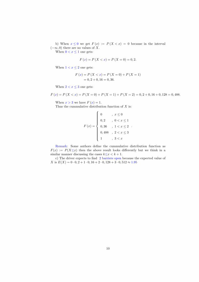
b) When 𝑥 ≤ 0 we get 𝐹 (𝑥) := 𝑃 (𝑋 < 𝑥) = 0 because in the interval(−∞, 0) there are no values of 𝑋.

When 0 < 𝑥 ≤ 1 one gets:

𝐹 (𝑥) = 𝑃 (𝑋 < 𝑥) = 𝑃 (𝑋 = 0) = 0, 2.

When 1 < 𝑥 ≤ 2 one gets:

𝐹 (𝑥) = 𝑃 (𝑋 < 𝑥) = 𝑃 (𝑋 = 0) + 𝑃 (𝑋 = 1)

= 0, 2 + 0, 16 = 0, 36.

When 2 < 𝑥 ≤ 3 one gets:

𝐹 (𝑥) = 𝑃 (𝑋 < 𝑥) = 𝑃 (𝑋 = 0) + 𝑃 (𝑋 = 1) + 𝑃 (𝑋 = 2) = 0, 2 + 0, 16 + 0, 128 = 0, 488.

When 𝑥 > 3 we have 𝐹 (𝑥) = 1.Thus the cummulative distribution function of 𝑋 is:

𝐹 (𝑥) =

⎧⎪⎪⎪⎪⎪⎪⎪⎪⎪⎨⎪⎪⎪⎪⎪⎪⎪⎪⎪⎩

0 , 𝑥 ≤ 0

0, 2 , 0 < 𝑥 ≤ 1

0, 36 , 1 < 𝑥 ≤ 2

0, 488 , 2 < 𝑥 ≤ 3

1 , 3 < 𝑥

.

Remark: Some authors define the cummulative distribution function as𝐹 (𝑥) := 𝑃 (𝑋≤𝑥) then the above result looks differently but we think in asimilar manner discussing the cases 𝑘≤𝑥 < 𝑘 + 1.

c) The driver expects to find 2 barriers open because the expected value of𝑋 is 𝐸(𝑋) = 0 · 0, 2 + 1 · 0, 16 + 2 · 0, 128 + 3 · 0, 512 ≈ 1.95

10

Proposed problems

Problem 1. From a lot of 100 items, of which 10 are defective a random sampleof size 5 is selected for quality control. Construct the distribution series of therandom number 𝑋 of defective items contained in the sample.

Problem 2. A car has four traffic lights on its route. Each of them allows itto move ahead or stop with the probability 0.5. Sketch the distribution polygonof the probabilities of the numbers of lights passed by the car before the first stophas occurred.

Problem 3. Births in a hospital occur randomly at an average rate of 1.8 birthsper hour. What is the probability of observing 4 births in a given hour at thehospital?

Problem 4. It is known that 3% of the circuit boards from a production line aredefective. If a random sample of 120 circuit boards is taken from this productionline estimate the probability that the sample contains:

i) Exactly 2 defective boards.

ii) At least 2 defective boards.

Problem 5. Four different prizes are randomly put into boxes of cereal. One ofthe prizes is a free ticket to the local zoo. Suppose that a family of four decides tobuy this cereal until obtaining four free tickets to the zoo. What is the probabilitythat the family will have to buy 10 boxes of cereal to obtain the four free ticketsto the zoo? What is the probability that the family will have to buy 16 boxes ofcereal to obtain the four free tickets to the zoo?

Problem 6. An automatic line in a state of normal adjustment can produce adefective item with probability 𝑝. The readjustment of the line is made immedi-ately after the first defective item has been produced. Find the average numberof items produced between two readjustments of the line.

Problem 7. For two independent random variables:

𝑋 :

⎛⎝0 1 2 3

18

38

28

28

⎞⎠and:

𝑌 :

⎛⎝0 1 2

12

14

14

⎞⎠compute 𝑋 + 𝑌, 2𝑋, 𝑀(𝑋) and show that 𝑀(𝑋𝑌 ) = 𝑀(𝑋)𝑀(𝑌 ). Compute𝑣𝑎𝑟(𝑋 + 2𝑌 ).

11

Problem 8. A student takes a multiple-choice test consisting of two problems.The first one has 3 possible answers and the second one has 5. The studentchooses, at random, one answer as the right one from each of the two pro-blems. Find the expected number 𝐸(𝑋) of right answers 𝑋 of the student. Findthe variance 𝑣𝑎𝑟(𝑋). Generalize.

Problem 9. The number of calls coming per minute into a hotels reservationcenter is a Poisson random variable of parameter 𝜆 = 3.

(a) Find the probability that no calls come in a given 1 minute period.(b) Assume that the number of calls arriving in two different minutes are

independent. Find the probability that at least two calls will arrive in a giventwo minute period.

(c) What is the expected number of calls in a given period of 1 minute ?

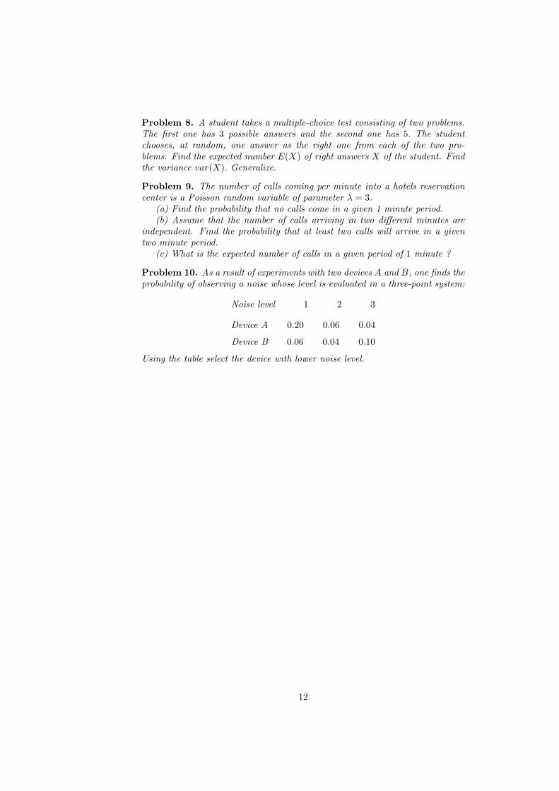
Problem 10. As a result of experiments with two devices 𝐴 and 𝐵, one finds theprobability of observing a noise whose level is evaluated in a three-point system:

Noise level 1 2 3

Device A 0.20 0.06 0.04

Device B 0.06 0.04 0.10

Using the table select the device with lower noise level.

12