Discrete Random Variables 93 Copyright © 2013 Pearson Education, Inc. Discrete Random Variables 4.2 A discrete variable can assume a countable number of values while a continuous random variable can assume values corresponding to any point in one or more intervals. 4.4 a. The amount of flu vaccine in a syringe is measured on an interval, so this is a continuous random variable. b. The heart rate (number of beats per minute) of an American male is countable, starting at whatever number of beats per minute is necessary for survival up to the maximum of which the heart is capable. That is, if m is the minimum number of beats necessary for survival, x can take on the values (m, m + 1, m + 2, ...) and is a discrete random variable. c. The time necessary to complete an exam is continuous as it can take on any value 0 ≤ x ≤ L, where L = limit imposed by instructor (if any). d. Barometric (atmospheric) pressure can take on any value within physical constraints, so it is a continuous random variable. e. The number of registered voters who vote in a national election is countable and is therefore discrete. f. An SAT score can take on only a countable number of outcomes, so it is discrete. 4.6 The values x can assume are 1, 2, 3, 4, or 5. Thus, x is a discrete random variable. 4.8 Since hertz could be any value in an interval, this variable is continuous. 4.10 The number of prior arrests could take on values 0, 1, 2, .. . Thus, x is a discrete random variable. 4.12 Answers will vary. An example of a discrete random variable of interest to a sociologist might be the number of times a person has been married. 4.14 Answers will vary. An example of a discrete random variable of interest to an art historian might be the number of times a piece of art has been restored. 4.16 a. x may take on the values −4, 0, 1, or 3. b. The value 1 is more likely than any of the other three since its probability of .4 is the maximum probability of the probability distribution. c. P(x > 0) = P(x = 1) + P(x = 3) = .4 + .3 = .7 d. P(x = −2) = 0 Chapter 4

Welcome message from author
This document is posted to help you gain knowledge. Please leave a comment to let me know what you think about it! Share it to your friends and learn new things together.
Transcript
Discrete Random Variables 93
Copyright © 2013 Pearson Education, Inc.
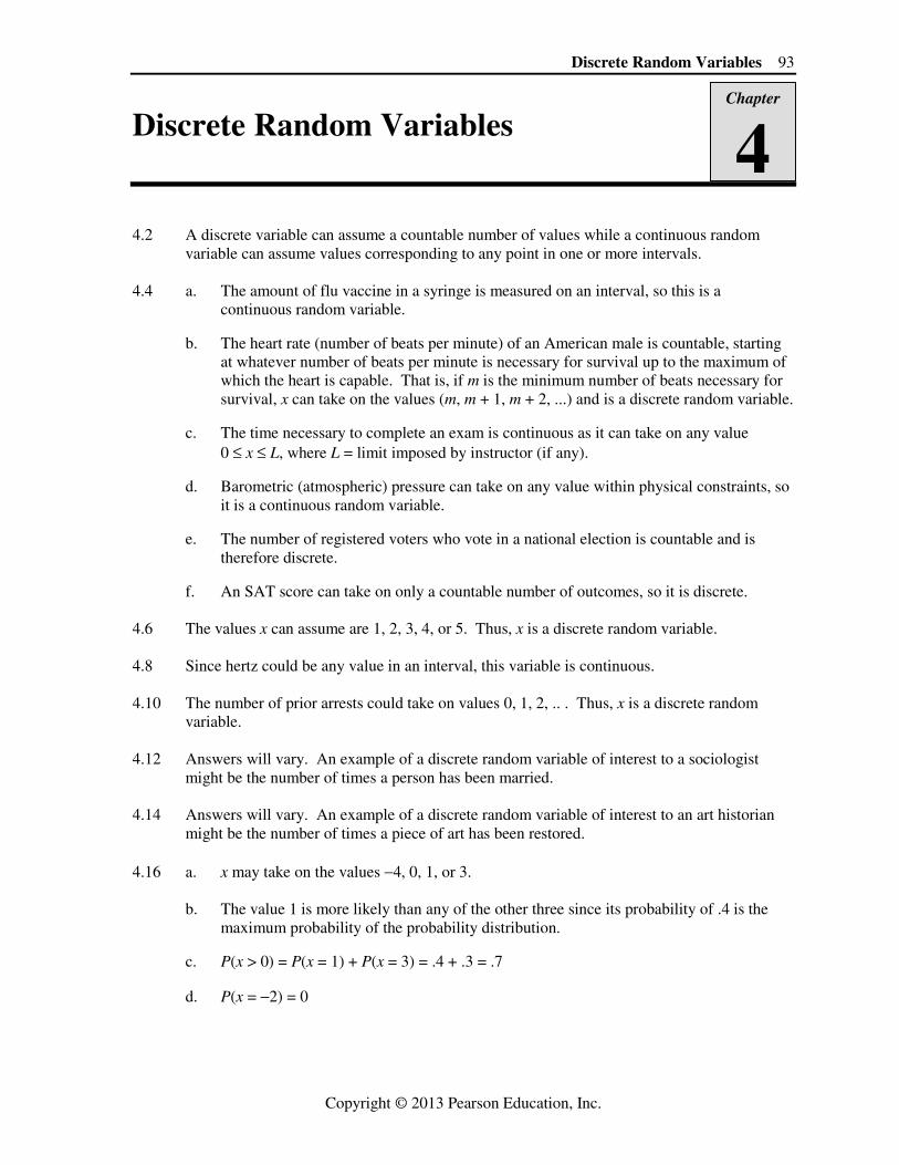
Discrete Random Variables 4.2 A discrete variable can assume a countable number of values while a continuous random
variable can assume values corresponding to any point in one or more intervals. 4.4 a. The amount of flu vaccine in a syringe is measured on an interval, so this is a
continuous random variable. b. The heart rate (number of beats per minute) of an American male is countable, starting
at whatever number of beats per minute is necessary for survival up to the maximum of which the heart is capable. That is, if m is the minimum number of beats necessary for survival, x can take on the values (m, m + 1, m + 2, ...) and is a discrete random variable.
c. The time necessary to complete an exam is continuous as it can take on any value 0 ≤ x ≤ L, where L = limit imposed by instructor (if any). d. Barometric (atmospheric) pressure can take on any value within physical constraints, so
it is a continuous random variable. e. The number of registered voters who vote in a national election is countable and is
therefore discrete. f. An SAT score can take on only a countable number of outcomes, so it is discrete. 4.6 The values x can assume are 1, 2, 3, 4, or 5. Thus, x is a discrete random variable. 4.8 Since hertz could be any value in an interval, this variable is continuous. 4.10 The number of prior arrests could take on values 0, 1, 2, .. . Thus, x is a discrete random
variable. 4.12 Answers will vary. An example of a discrete random variable of interest to a sociologist
might be the number of times a person has been married. 4.14 Answers will vary. An example of a discrete random variable of interest to an art historian
might be the number of times a piece of art has been restored. 4.16 a. x may take on the values −4, 0, 1, or 3. b. The value 1 is more likely than any of the other three since its probability of .4 is the
maximum probability of the probability distribution. c. P(x > 0) = P(x = 1) + P(x = 3) = .4 + .3 = .7
d. P(x = −2) = 0
Chapter
4
94 Chapter 4
Copyright © 2013 Pearson Education, Inc.
4.18 a. This is a valid distribution because ( ) .2 .3 .3 .2 1p x = + + + =∑ and ( ) 0p x ≥ for all
values of x.
b. This is not a valid distribution because ( ) .25 .50 .20 .95 1p x = + + = ≠∑ . c. This is not a valid distribution because one of the probabilities is negative.
d. This is not a valid distribution because ( ) .15 .20 .40 .35 1.10 1p x = + + + = ≠∑ .
4.20 a. P(x ≤ 0) = P(x = −2) + P(x = −1) + P(x = 0) = .10 + .15 + .40 = .65 b. P(x > −1) = P(x = 0) + P(x = 1) + P(x = 2) = .40 + .30 + .05 = .75 c. P(−1 ≤ x ≤ 1) = P(x = −1) + P(x = 0) + P(x = 1) = .15 + .40 + .30 = .85 d. P(x < 2) = 1 − P(x = 2) = 1 − .05 = .95 e. P(−1 < x < 2) = P(x = 0) + P(x = 1) = .40 + .30 = .70 f. P(x < 1) = P(x = −2) + P(x = −1) + P(x = 0) = .10 + .15 + .40 = .65 4.22 a. To find the probabilities, we divide the percents by 100. In tabular form, the probability
distribution for x, the driver-side star rating, is:
x 1 2 3 4 5
p(x) .0000 .0408 .1735 .6020 .1837
b. P(x = 5) = .1837
c. P(x ≤ 2) = P(x = 1) + P(x = 2) = 0 + .0408 = .0408 4.24 a. To find probabilities, change the percents given in the table to proportions by dividing
by 100. The probability distribution for x is:
x 1 2 3 4 p(x) .40 .54 .02 .04
b. P(x ≥ 3) = P(x = 3) + P(x = 4) = .02 + .04 = .06. 4.26 a. The number of solar energy cells out of 5 that are manufactured in China, x, can take on
values 0, 1, 2, 3, or 5. Thus, x is a discrete random variable.
b. 0 5 0 5(5!)(.35) (.65) (5)(4)(3)(2)(1)(.65)
(0) .1160(0!)(5 0)! 1(5)(4)(3)(2)(1)
p−
= = =−
1 5 1 4(5!)(.35) (.65) (5)(4)(3)(2)(1)(.35)(.65)
(1) .3124(1!)(5 1)! 1(4)(3)(2)(1)
p−
= = =−
Discrete Random Variables 95
Copyright © 2013 Pearson Education, Inc.
2 5 2 2 3(5!)(.35) (.65) (5)(4)(3)(2)(1)(.35) (.65)
(2) .3364(2!)(5 2)! (2)(1)(3)(2)(1)
p−
= = =−
3 5 3 3 2(5!)(.35) (.65) (5)(4)(3)(2)(1)(.35) (.65)
(3) .1811(3!)(5 3)! (3)(2)(1)(2)(1)
p−
= = =−
4 5 4 4(5!)(.35) (.65) (5)(4)(3)(2)(1)(.35) (.65)
(4) .0488(4!)(5 4)! (4)(3)(2)(1)(1)
p−
= = =−
5 5 5 5(5!)(.35) (.65) (5)(4)(3)(2)(1)(.35)
(5) .0053(5!)(5 5)! (5)(4)(3)(2)(1)(1)
p−
= = =−
c. The properties of a discrete probability distribution are: 0 ( ) 1p x≤ ≤ for all values of x
and ( ) 1p x =∑ . All of the probabilities in part b are greater than 0. The sum of the
probabilities is ( ) .1160 .3124 .3364 .1811 .0488 .0053 1.p x = + + + + + =∑
d. ( 4) (4) (5) .0488 .0053 .0541P x p p≥ = + = + = 4.28 The probability distribution of x is:
(8.5) .000123 .008823 .128030 .325213 .462189
(9.0) .000456 .020086 .153044 .115178 .288764
(9.5) .001257 .032014 .108400 .141671
(10.0) .002514 .032901 .034552 .069967
(10.5) .003561 .021675 .025236
p
p
p
p
p
= + + + =
= + + + =
= + + =
= + + =
= + =
(11.0) .003401 .006284 .001972 .011657
(12.0) .000518
p
p
= + + =
=
96 Chapter 4
Copyright © 2013 Pearson Education, Inc.
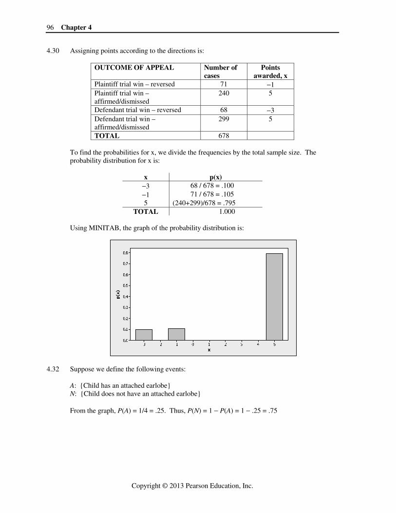
4.30 Assigning points according to the directions is:
OUTCOME OF APPEAL Number of cases
Points awarded, x
Plaintiff trial win – reversed 71 −1 Plaintiff trial win – affirmed/dismissed
240 5
Defendant trial win – reversed 68 −3 Defendant trial win – affirmed/dismissed
299 5
TOTAL 678
To find the probabilities for x, we divide the frequencies by the total sample size. The probability distribution for x is:
x p(x)
−3 68 / 678 = .100 −1 71 / 678 = .105 5 (240+299)/678 = .795
TOTAL 1.000 Using MINITAB, the graph of the probability distribution is:
x
p(
x)
543210-1-2-3
0.8
0.7
0.6
0.5
0.4
0.3
0.2
0.1
0.0
4.32 Suppose we define the following events: A: {Child has an attached earlobe} N: {Child does not have an attached earlobe} From the graph, P(A) = 1/4 = .25. Thus, P(N) = 1 − P(A) = 1 − .25 = .75
Discrete Random Variables 97
Copyright © 2013 Pearson Education, Inc.
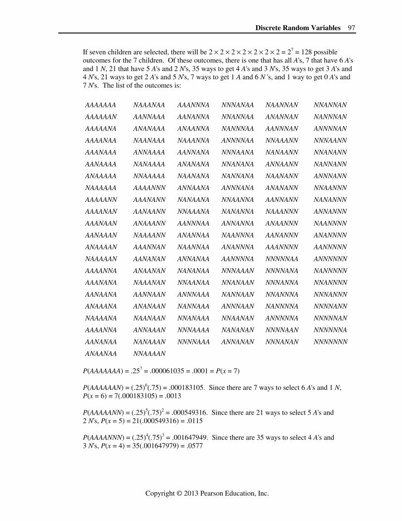
If seven children are selected, there will be 2 × 2 × 2 × 2 × 2 × 2 × 2 = 27 = 128 possible outcomes for the 7 children. Of these outcomes, there is one that has all A's, 7 that have 6 A's and 1 N, 21 that have 5 A's and 2 N's, 35 ways to get 4 A's and 3 N's, 35 ways to get 3 A's and 4 N's, 21 ways to get 2 A's and 5 N's, 7 ways to get 1 A and 6 N 's, and 1 way to get 0 A's and 7 N's. The list of the outcomes is:
AAAAAAA NAAANAA AAANNNA NNNANAA NAANNAN NNANNAN
AAAAAAN AANNAAA AANANNA NNANNAA ANANNAN NANNNAN
AAAAANA ANANAAA ANAANNA NANNNAA AANNNAN ANNNNAN
AAAANAA NAANAAA NAAANNA ANNNNAA NNAAANN NNNAANN
AAANAAA ANNAAAA AANNANA NNNAANA NANAANN NNANANN
AANAAAA NANAAAA ANANANA NNANANA ANNAANN NANNANN
ANAAAAA NNAAAAA NAANANA NANNANA NAANANN ANNNANN
NAAAAAA AAAANNN ANNAANA ANNNANA ANANANN NNAANNN
AAAAANN AAANANN NANAANA NNAANNA AANNANN NANANNN
AAAANAN AANAANN NNAAANA NANANNA NAAANNN ANNANNN
AAANAAN ANAAANN AANNNAA ANNANNA ANAANNN NAANNNN
AANAAAN NAAAANN ANANNAA NAANNNA AANANNN ANANNNN
ANAAAAN AAANNAN NAANNAA ANANNNA AAANNNN AANNNNN
NAAAAAN AANANAN ANNANAA AANNNNA NNNNNAA ANNNNNN
AAAANNA ANAANAN NANANAA NNNAAAN NNNNANA NANNNNN
AAANANA NAAANAN NNAANAA NNANAAN NNNANNA NNANNNN
AANAANA AANNAAN ANNNAAA NANNAAN NNANNNA NNNANNN
ANAAANA ANANAAN NANNAAA ANNNAAN NANNNNA NNNNANN
NAAAANA NAANAAN NNANAAA NNAANAN ANNNNNA NNNNNAN
AAAANNA ANNAAAN NNNAAAA NANANAN NNNNAAN NNNNNNA
AANANAA NANAAAN NNNNAAA ANNANAN NNNANAN NNNNNNN
ANAANAA NNAAAAN P(AAAAAAA) = .257 = .000061035 = .0001 = P(x = 7) P(AAAAAAN) = (.25)6(.75) = .000183105. Since there are 7 ways to select 6 A's and 1 N, P(x = 6) = 7(.000183105) = .0013 P(AAAAANN) = (.25)5(.75)2 = .000549316. Since there are 21 ways to select 5 A's and 2 N's, P(x = 5) = 21(.000549316) = .0115 P(AAAANNN) = (.25)4(.75)3 = .001647949. Since there are 35 ways to select 4 A's and 3 N's, P(x = 4) = 35(.001647979) = .0577
98 Chapter 4
Copyright © 2013 Pearson Education, Inc.
P(AAANNNN) = (.25)3(.75)4 = .004943847. Since there are 35 ways to select 3 A's and 4 N's, P(x = 3) = 35(.004943847) = .1730 P(AANNNNN) = (.25)2(.75)5 = .014831542. Since there are 21 ways to select 2 A's and 5 N's, P(x = 2) = 21(.014831542) = .3115 P(ANNNNNN) = (.25)(.75)6 = .044494628. Since there are 7 ways to select 1 A's and 6 N's, P(x = 1) = 7(.044494628) = .3115 P(NNNNNNN) = (.75)7 = .133483886. Since there is 1 way to select 0 A's and 7 N's, P(x = 0) = .1335 4.34 The expected value of a random variable represents the mean of the probability distribution.
You can think of the expected value as the mean value of x in a very large (actually, infinite) number of repetitions of the experiment.
4.36 For a mound-shaped, symmetric distribution, the probability that x falls in the interval μ ± 2σ
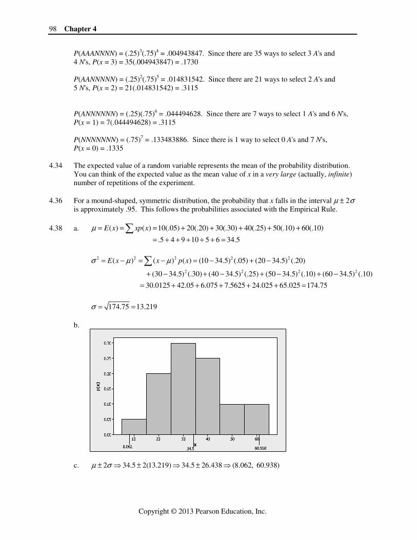
is approximately .95. This follows the probabilities associated with the Empirical Rule. 4.38 a. ( ) ( ) 10(.05) 20(.20) 30(.30) 40(.25) 50(.10) 60(.10)E x xp xμ = = = + + + + +∑
.5 4 9 10 5 6 34.5= + + + + + =
2 2 2 2 2
2 2 2 2
( ) ( ) ( ) (10 34.5) (.05) (20 34.5) (.20)
(30 34.5) (.30) (40 34.5) (.25) (50 34.5) (.10) (60 34.5) (.10)
30.0125 42.05 6.075 7.5625 24.025 65.025 174.75
E x x p xσ μ μ= − = − = − + −
+ − + − + − + −= + + + + + =
∑
174.75 13.219σ = = b.
x
p(
x)
605040302010
0.30
0.25
0.20
0.15
0.10
0.05
0.00
8.06234.5 60.938
c. 2 34.5 2(13.219) 34.5 26.438 (8.062, 60.938)μ σ± ⇒ ± ⇒ ± ⇒
Discrete Random Variables 99
Copyright © 2013 Pearson Education, Inc.
( ) ( ) ( ) ( ) ( ) ( ) ( )8.062 60.938 10 20 30 40 50 60
.05 .20 .30 .25 .10 .10 1.00
P x p p p p p p< < = + + + + += + + + + + =
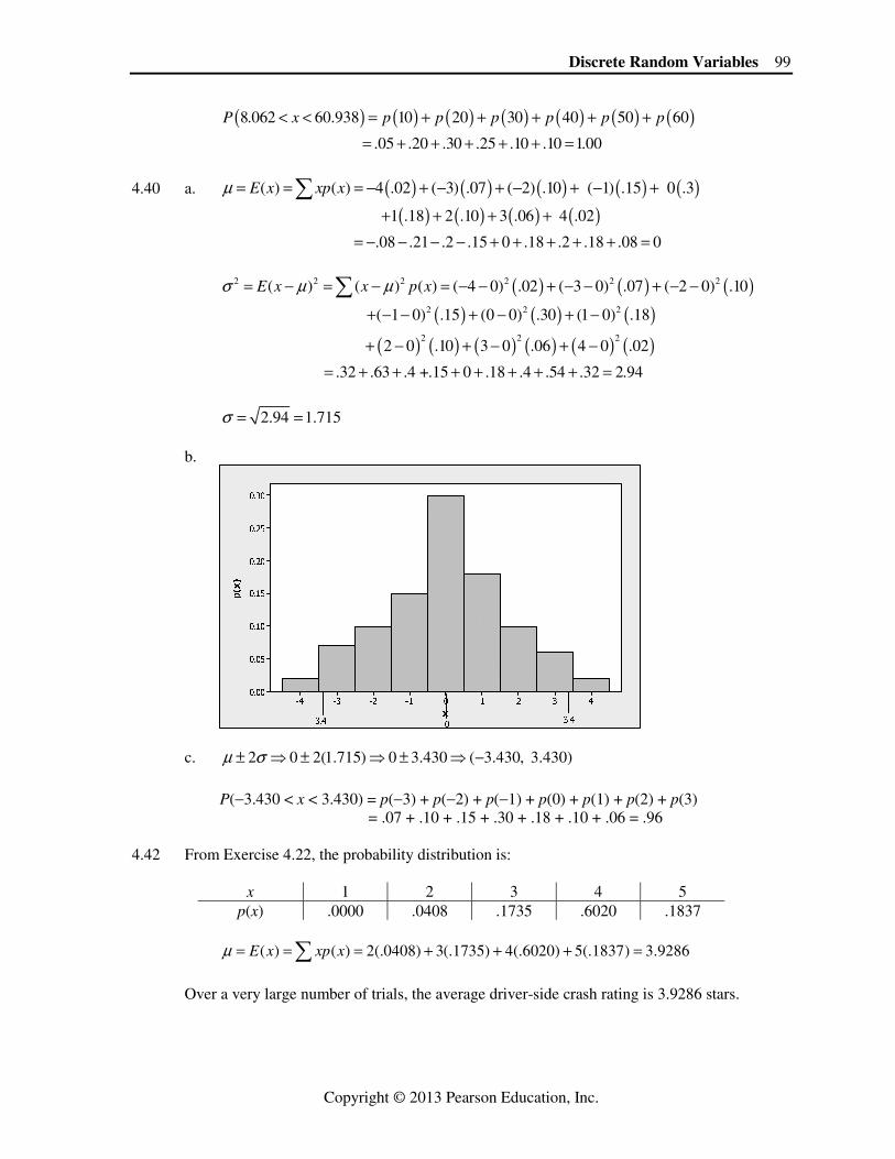
4.40 a. ( ) ( ) ( ) ( ) ( )( ) ( ) 4 .02 ( 3) .07 ( 2) .10 ( 1) .15 0 .3E x xp xμ = = = − + − + − + − +∑
( ) ( ) ( ) ( ) 1 .18 2 .10 3 .06 4 .02
.08 .21 .2 .15 0 .18 .2 .18 .08 0
+ + + += − − − − + + + + + =
( ) ( ) ( )( ) ( ) ( )
( ) ( ) ( ) ( ) ( ) ( )
2 2 2 2 2 2
2 2 2
2 2 2
( ) ( ) ( ) ( 4 0) .02 ( 3 0) .07 ( 2 0) .10
( 1 0) .15 (0 0) .30 (1 0) .18
2 0 .10 3 0 .06 4 0 .02
.32 .63 .4 +.15 0 .18 .4 .54 .32 2.94
E x x p xσ μ μ= − = − = − − + − − + − −
+ − − + − + −
+ − + − + −= + + + + + + + =
∑
2.94 1.715σ = = b.
x
p(
x)
43210-1-2-3-4
0.30
0.25
0.20
0.15
0.10
0.05
0.00
0-3.4
3
3.4 c. 2 0 2(1.715) 0 3.430 ( 3.430, 3.430)μ σ± ⇒ ± ⇒ ± ⇒ − P(−3.430 < x < 3.430) = p(−3) + p(−2) + p(−1) + p(0) + p(1) + p(2) + p(3) = .07 + .10 + .15 + .30 + .18 + .10 + .06 = .96 4.42 From Exercise 4.22, the probability distribution is:
x 1 2 3 4 5 p(x) .0000 .0408 .1735 .6020 .1837
( ) ( ) 2(.0408) 3(.1735) 4(.6020) 5(.1837) 3.9286E x xp xμ = = = + + + =∑
Over a very large number of trials, the average driver-side crash rating is 3.9286 stars.
100 Chapter 4
Copyright © 2013 Pearson Education, Inc.
4.44 ( ) ( ) 1(.40) 2(.54) 3(.02) 4(.04) .40 1.08 .06 .16 1.70E x xp xμ = = = + + + = + + + =∑
The average number of insect eggs on a blade of water hyacinth is 1.70. 4.46 Let x = winnings in the Florida lottery. The probability distribution for x is:
x p(x) −$1 22,999,999/23,000,000
$6,999,999 1/23,000,000
The expected net winnings would be: ( ) ( 1)(22,999,999 / 23,000,000) 6,999,999(1 / 23,000,000) $.70E xμ = = − + = − The average winnings of all those who play the lottery is −$.70. 4.48 a. Since there are 20 possible outcomes that are all equally likely, the probability of any of
the 20 numbers is 1/20. The probability distribution of x is:
P(x = 5) = 1/20 = .05; P(x = 10) = 1/20 = .05; etc.
x 5 10 15 20 25 30 35 40 45 50 55 60 65 70 75 80 85 90 95 100
p(x) .05 .05 .05 .05 .05 .05 .05 .05 .05 .05 .05 .05 .05 .05 .05 .05 .05 .05 .05 .05
b. ( ) ( ) ( ) ( )2 2( ) ( ) (5 52.5) .05 (10 52.5) .05 15 .05 20 .05E x xp x= = − + − + +∑
( ) ( ) ( ) ( ) ( ) ( ) ( ) ( )( ) ( ) ( ) ( ) ( ) ( ) ( ) ( )
25 .05 30 .05 35 .05 40 .05 45 .05 50 .05 55 .05 60 .05
65 .05 70 .05 75 .05 80 .05 85 .05 90 .05 95 .05 100 .05
52.5
+ + + + + + + +
+ + + + + + + +=
c. ( ) ( )2 2 2 2 2( ) ( ) ( ) (5 52.5) .05 (10 52.5) .05E x x p xσ μ μ= − = − = − + −∑
( ) ( ) ( ) ( )( ) ( ) ( ) ( )( ) ( ) ( ) ( )( ) ( )
2 2 2 2
2 2 2 2
2 2 2 2
2 2
(15 52.5) .05 (20 52.5) .05 (25 52.5) .05 (30 52.5) .05
(35 52.5) .05 (40 52.5) .05 (45 52.5) .05 (50 52.5) .05
(55 52.5) .05 (60 52.5) .05 (65 52.5) .05 (70 52.5) .05
(75 52.5) .05 (80 52.5) .05 (85
+ − + − + − + −
+ − + − + − + −
+ − + − + − + −
+ − + − + ( ) ( )( ) ( )
2 2
2 2
52.5) .05 (90 52.5) .05
(95 52.5) .05 (100 52.5) .05
831.25
− + −
+ − + −=
2 831.25 28.83σ σ= = = Since the uniform distribution is not mound-shaped, we will use Chebyshev's theorem
to describe the data. We know that at least 8/9 of the observations will fall with 3 standard deviations of the mean and at least 3/4 of the observations will fall within 2 standard deviations of the mean. For this problem,
( )2 52.5 2 28.83 52.5 57.66 ( 5.16, 110.16)μ σ± ⇒ ± ⇒ ± ⇒ − . Thus, at least 3/4 of the
data will fall between −5.16 and 110.16. For our problem, all of the observations will
Discrete Random Variables 101
Copyright © 2013 Pearson Education, Inc.
fall within 2 standard deviations of the mean. Thus, x is just as likely to fall within any interval of equal length.
d. If a player spins the wheel twice, the total number of outcomes will be 20(20) = 400.
The sample space is:
5, 5 10, 5 15, 5 20, 5 25, 5... 100, 55,10 10,10 15,10 20,10 25,10... 100,10
5,15 10,15 15,15 20,15 25,15... 100,15. . .
. . . . . .
... ...
... 5,100 10,100 15,100 20,100 25,100... 100,100
Each of these outcomes are equally likely, so each has a probability of 1/400 = .0025. Now, let x equal the sum of the two numbers in each sample. There is one sample with
a sum of 10, two samples with a sum of 15, three samples with a sum of 20, etc. If the sum of the two numbers exceeds 100, then x is zero. The probability distribution of x is:
x p(x)
0 .5250
10 .0025
15 .0050
20 .0075 25 .0100
30 .0125
35 .0150
40 .0175 45 .0200
50 .0225
55 .0250
60 .0275 65 .0300
70 .0325
75 .0350
80 .0375 85 .0400
90 .0425
95 .0450
100 .0475 e. We assumed that the wheel is fair, or that all outcomes are equally likely.
102 Chapter 4
Copyright © 2013 Pearson Education, Inc.
f. ( ) ( ) ( ) ( ) ( )( ) ( ) 0 .5250 10 .0025 15 .0050 20 .0075 ... 100 .0475
33.25
E x xp xμ = = = + + + + +
=∑
( ) ( )( ) ( ) ( )
2 2 2 2 2
2 2 2
( ) ( ) ( ) (0 33.25) .525 (10 33.25) .0025
(15 33.25) .0050 (20 33.25) .0075 ... (100 33.25) .0475
1471.3125
E x x p xσ μ μ= − = − = − + −
+ − + − + + −=
∑
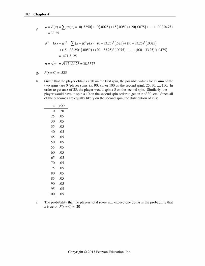
2 1471.3125 38.3577σ σ= = = g. P(x = 0) = .525 h. Given that the player obtains a 20 on the first spin, the possible values for x (sum of the
two spins) are 0 (player spins 85, 90, 95, or 100 on the second spin), 25, 30, ..., 100. In order to get an x of 25, the player would spin a 5 on the second spin. Similarly, the player would have to spin a 10 on the second spin order to get an x of 30, etc. Since all of the outcomes are equally likely on the second spin, the distribution of x is:
x p(x)
0 .20
25 .05 30 .05
35 .05
40 .05
45 .05 50 .05
55 .05
60 .05
65 .05 70 .05
75 .05
80 .05
85 .05 90 .05
95 .05
100 .05
i. The probability that the players total score will exceed one dollar is the probability that x is zero. P(x = 0) = .20

Discrete Random Variables 103
Copyright © 2013 Pearson Education, Inc.
j. Given that the player obtains a 65 on the first spin, the possible values for x (sum of the two spins) are 0 (player spins 40, 45, 50, up to 100 on second spin), 70, 75, 80,..., 100. In order to get an x of 70, the player would spin a 5 on the second spin. Similarly, the player would have to spin a 10 on the second spin in order to get an x of 75, etc. Since all of the outcomes are equally likely on the second spin, the distribution of x is:
x p(x)
0 .65 70 .05
75 .05
80 .05 85 .05
90 .05
95 .05
100 .05
The probability that the players total score will exceed one dollar is the probability that x is zero. P(x = 0) = .65.
k. There are many possible answers. Notice that P(x = 0) on the second spin is equal to
the value on the first spin divided by 100. If a player got a 20 on the first spin, then P(x = 0) on the second spin is 20/100 = .20. If a player got a 65 on the first spin, then P(x = 0) on the second spin is 65/100 = .65.
4.50 The five characteristics of a binomial random variable are:
a. The experiment consists of n identical trials. b. There are only two possible outcomes on each trial. We will denote one outcome by S
(for Success) and the other by F (for Failure). c. The probability of S remains the same from trial to trial. This probability is denoted by
p, and the probability of F is denoted by q. Note that q = 1 – p. d. The trials are independent. e. The binomial random variable x is the number of S’s in n trials.
4.52 a. There are n = 5 trials.
b. The value of p is p = .7.
4.54 a. ( )( )0 5 0 0 55 5! 5 4 3 2 1(0) (.7) (.3) (.7) (.3) 1 .00243 .00243
0 0!5! 1 5 4 3 2 1p −⎛ ⎞ ⋅ ⋅ ⋅ ⋅= = = =⎜ ⎟ ⋅ ⋅ ⋅ ⋅ ⋅⎝ ⎠
1 5 1 1 45 5!(1) (.7) (.3) (.7) (.3) .02835
1 1!4!p −⎛ ⎞
= = =⎜ ⎟⎝ ⎠
104 Chapter 4
Copyright © 2013 Pearson Education, Inc.
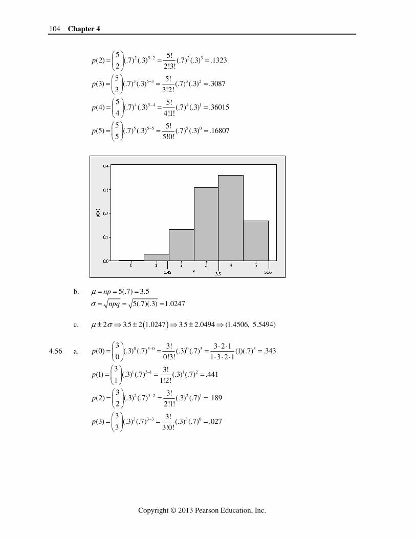
2 5 2 2 35 5!(2) (.7) (.3) (.7) (.3) .1323
2 2!3!p −⎛ ⎞
= = =⎜ ⎟⎝ ⎠
3 5 3 3 25 5!(3) (.7) (.3) (.7) (.3) .3087
3 3!2!p −⎛ ⎞
= = =⎜ ⎟⎝ ⎠
4 5 4 4 15 5!(4) (.7) (.3) (.7) (.3) .36015
4 4!1!p −⎛ ⎞
= = =⎜ ⎟⎝ ⎠
5 5 5 5 05 5!(5) (.7) (.3) (.7) (.3) .16807
5 5!0!p −⎛ ⎞
= = =⎜ ⎟⎝ ⎠
x
p(
x)
543210
0.4
0.3
0.2
0.1
0.0
3.51.45 5.55
b. 5(.7) 3.5npμ = = =
5(.7)(.3) 1.0247npqσ = = =
c. ( )2 3.5 2 1.0247 3.5 2.0494 (1.4506, 5.5494)μ σ± ⇒ ± ⇒ ± ⇒
4.56 a. 0 3 0 0 3 33 3! 3 2 1(0) (.3) (.7) (.3) (.7) (1)(.7) .343
0 0!3! 1 3 2 1p −⎛ ⎞ ⋅ ⋅= = = =⎜ ⎟ ⋅ ⋅ ⋅⎝ ⎠
1 3 1 1 23 3!(1) (.3) (.7) (.3) (.7) .441
1 1!2!p −⎛ ⎞
= = =⎜ ⎟⎝ ⎠
2 3 2 2 13 3!(2) (.3) (.7) (.3) (.7) .189
2 2!1!p −⎛ ⎞
= = =⎜ ⎟⎝ ⎠
3 3 3 3 03 3!(3) (.3) (.7) (.3) (.7) .027
3 3!0!p −⎛ ⎞
= = =⎜ ⎟⎝ ⎠
Discrete Random Variables 105
Copyright © 2013 Pearson Education, Inc.
b. x p(x) 0 .343
1 .441 2 .189
3 .027
4.58 a. P(x = 2) = P(x ≤ 2) − P(x ≤ 1) = .167 − .046 = .121 (from Table II, Appendix A) b. P(x ≤ 5) = .034 c. P(x > 1) = 1 − P(x ≤ 1) = 1 − .919 = .081 4.60 a. The simple events listed below are all equally likely, implying a probability of 1/32 for
each. The list is in a regular pattern such that the first simple event would yield x = 0, the next five yield x = 1, the next ten yield x = 2, the next ten also yield x = 3, the next five yield x = 4, and the final one yields x = 5. The resulting probability distribution is given below the simple events.
, , , , , , ,
, , , , , , ,
, , , , , , ,
, , , , ,
FFFFF FFFFS FFFSF FFSFF FSFFF SFFFF FFFSS FFSFS
FSFFS SFFFS FFSSF FSFSF SFFSF FSSFF SFSFF SSFFF
FFSSS FSFSS SFFSS FSSFS SFSFS SSFFS FSSSF SFSSF
SSFSF SSSFF FSSSS SFSSS SSFSS SSS , , FS SSSSF SSSSS
⎡ ⎤⎢ ⎥⎢ ⎥⎢ ⎥⎢ ⎥⎣ ⎦
x 0 1 2 3 4 5
p(x) 1/32 5/32 10/32 10/32 5/32 1/32
b. ( ) ( )0 50 5 0 55 5! 5 4 3 2 1( 0) (.5) (.5) .5 .5 (1)(.5) .03125
0 0!5! 1 5 4 3 2 1P x −⎛ ⎞ ⋅ ⋅ ⋅ ⋅= = = = =⎜ ⎟ ⋅ ⋅ ⋅ ⋅ ⋅⎝ ⎠
( ) ( )1 41 5 1 55 5! 5 4 3 2 1
( 1) (.5) (.5) .5 .5 (.5) .156251 1!4! 1 4 3 2 1
P x −⎛ ⎞ ⋅ ⋅ ⋅ ⋅= = = = =⎜ ⎟ ⋅ ⋅ ⋅ ⋅⎝ ⎠
( ) ( )2 32 5 2 55 5! 5 4 3 2 1( 2) (.5) (.5) .5 .5 (.5) .3125
2 2!3! 2 1 3 2 1P x −⎛ ⎞ ⋅ ⋅ ⋅ ⋅= = = = =⎜ ⎟ ⋅ ⋅ ⋅ ⋅⎝ ⎠
( ) ( )3 23 5 3 55 5! 5 4 3 2 1
( 3) (.5) (.5) .5 .5 (.5) .31253 3!2! 3 2 1 2 1
P x −⎛ ⎞ ⋅ ⋅ ⋅ ⋅= = = = =⎜ ⎟ ⋅ ⋅ ⋅ ⋅⎝ ⎠
( ) ( )4 14 5 4 55 5! 5 4 3 2 1
( 4) (.5) (.5) .5 .5 (.5) .156254 4!1! 4 3 2 1 1
P x −⎛ ⎞ ⋅ ⋅ ⋅ ⋅= = = = =⎜ ⎟ ⋅ ⋅ ⋅ ⋅⎝ ⎠
( ) ( )5 05 5 5 55 5! 5 4 3 2 1
( 5) (.5) (.5) .5 .5 (.5) .031255 5!0! 5 4 3 2 1 1
P x −⎛ ⎞ ⋅ ⋅ ⋅ ⋅= = = = =⎜ ⎟ ⋅ ⋅ ⋅ ⋅ ⋅⎝ ⎠
106 Chapter 4
Copyright © 2013 Pearson Education, Inc.
4.62 a. For this exercise, a success will be an owner acquiring his/her next dog or cat from a shelter.
b. For this exercise, n = 10. c. For this exercise, p = .5. d. Using Table II, Appendix A, with n = 10 and p = .5, ( 7) ( 7) ( 6) .945 .828 .117P x P x P x= = ≤ − ≤ = − = e. Using Table II, Appendix A, with n = 10 and p = .5, ( 3) .172P x ≤ = f. Using Table II, Appendix A, with n = 10 and p = .5, ( 8) 1 ( 8) 1 .989 .011P x P x> = − ≤ = − = 4.64 a. We will check the characteristics of a binomial random variable: 1. This experiment consists of n = 5 identical trials.
2. There are only 2 possible outcomes for each trial. A brand of bottled water can use tap water (S) or not (F).
3. The probability of S remains the same from trial to trial. In this case, p = P(S) ≈ .25
for each trial.
4. The trials are independent. Since there are a finite number of brands of bottled water, the trials are not exactly independent. However, since the number of brands of bottled water is large compared to the sample size of 5, the trials are close enough to being independent.
5. x = number of brands of bottled water using tap water in 5 trials.
b. The formula for finding the binomial probabilities is:
55( ) .25 (.75)x xp x
x−⎛ ⎞
= ⎜ ⎟⎝ ⎠
for x = 0, 1, 2, 3, 4, 5
c. 2 5 2 2 35 5!( 2) (2) .25 (.75) .25 (.75) .2637
2 2!3!P x p −⎛ ⎞
= = = = =⎜ ⎟⎝ ⎠
d. 0 5 0 1 5 1
0 5 1 4
5 5( 1) (0) (1) .25 (.75) .25 (.75)
0 1
5! 5!.25 (.75) .25 (.75) .2373 .3955 .6328
0!5! 1!4!
P x p p − −⎛ ⎞ ⎛ ⎞≤ = + = +⎜ ⎟ ⎜ ⎟
⎝ ⎠ ⎝ ⎠
= + = + =
Discrete Random Variables 107
Copyright © 2013 Pearson Education, Inc.
4.66 a. Let x = number of births in 1,000 that take place by Caesarian section. ( ) ( )1000 .32 320.E x np= = =
b. 1000(.32)(.68) 14.7513npqσ = = =
c. Since p is not real small, the distribution of x will be fairly mound-shaped, so the
Empirical Rule will apply. We know that approximately 95% of the observations will fall within 2 standard deviations of the mean. Thus,
2 320 2(14.7513) 320 29.5026 (290.4974, 349.5026)μ σ± ⇒ ± ⇒ ± ⇒ In a sample of 1000 births, we would expect that somewhere between 291 and 349 will
be Caesarian section births. 4.68 a. Let x = number of students initially answering question correctly. Then x is a binomial
random variable with n = 20 and p = .5. Using Table II, Appendix A, ( 10) 1 ( 10) 1 .588 .412P x P x> = − ≤ = − = b. Let x = number of students answering question correctly after feedback. Then x is a
binomial random variable with n = 20 and p = .7. Using Table II, Appendix A, ( 10) 1 ( 10) 1 .048 .952P x P x> = − ≤ = − = 4.70 μ = E(x) = np = 50(.6) = 30.0
50(.6)(.4) 3.4641σ = =
Since p is not real small, the distribution of x will be fairly mound-shaped, so the Empirical
Rule will apply. We know that approximately 95% of the observations will fall within 2 standard deviations of the mean. Thus,
2 30 2(3.4641) 30 6.9282 (23.0718, 36.9282)μ σ± ⇒ ± ⇒ ± ⇒ 4.72 Let x = number of slaughtered chickens in 5 that passes inspection with fecal contamination. Then x is a binomial random variable with n = 5 and p = .01 (from Exercise 3.15.) P(x ≥ 1) = 1 – P(x = 0) = 1 − .951 = .049 (From Table II, Appendix A). 4.74 Let n = 20, p = .5, and x = number of correct questions in 20 trials. Then x has a binomial
distribution. We want to find k such that: P(x ≥ k) < .05 or 1 − P(x ≤ k − 1) < .05 ⇒ P(x ≤ k − 1) > .95 ⇒ k − 1 = 14 ⇒ k = 15 (from Table II, Appendix A) Note: P(x ≥ 14) = 1 − P(x ≤ 13) = 1 − .942 = .058 P(x ≥ 15) = 1 − P(x ≤ 14) = 1 − .979 = .021 Thus, to have the probability less than .05, the lowest passing grade should be 15.
108 Chapter 4
Copyright © 2013 Pearson Education, Inc.
4.76 Let x = Number of boys in 24 children. Then x is a binomial random variable with n = 24 and p = .5.
( ) 24(.5) 12E x npμ = = = =
24(.5)(.5) 6 2.4495npqσ = = = =
A value of 21 boys out of 24 children would have a z-score of 21 12
3.672.4495
z−= = . A value
that is 3.67 standard deviations above the mean would be highly unlikely. Thus, we would agree with the statement, “Rodgers men produce boys.”
4.78 For the Poisson probability distribution 1010
( ) ( 0,1,2,...)!
x ep x x
x
−= =
the value of λ is 10. 4.80 a. In order to graph the probability distribution, we need to know the probabilities for the
possible values of x. Using Table III of Appendix A, with λ = 10: p(0) = .000 p(1) = P(x ≤ 1) – P(x = 0) = .000 − .000 = .000 p(2) = P(x ≤ 2) – P(x ≤ 1) = .003 − .000 = .003 p(3) = P(x ≤ 3) – P(x ≤ 2) = .010 − .003 = .007 p(4) = P(x ≤ 4) – P(x ≤ 3) = .029 − .010 = .019 p(5) = P(x ≤ 5) – P(x ≤ 4) = .067 − .029 = .038 p(6) = P(x ≤ 6) – P(x ≤ 5) = .130 − .067 = .063 p(7) = P(x ≤ 7) – P(x ≤ 6) = .220 − .130 = .090 p(8) = P(x ≤ 8) – P(x ≤ 7) = .333 − .220 = .113 p(9) = P(x ≤ 9) – P(x ≤ 8) = .458 − .333 = .125 p(10) = P(x ≤ 10) – P(x ≤ 9) = .583 − .458 = .125 p(11) = P(x ≤ 11) – P(x ≤ 10) = .697 − .583 = .114 p(12) = P(x ≤ 12) – P(x ≤ 11) = .792 − .697 = .095 p(13) = P(x ≤ 13) – P(x ≤ 12) = .864 − .792 = .072 p(14) = P(x ≤ 14) – P(x ≤ 13) = .917 − .864 = .053 p(15) = P(x ≤ 15) – P(x ≤ 14) = .951 − .917 = .034 p(16) = P(x ≤ 16) – P(x ≤ 15) = .973 − .951 = .022 p(17) = P(x ≤ 17) – P(x ≤ 16) = .986 − .973 = .013 p(18) = P(x ≤ 18) – P(x ≤ 17) = .993 − .986 = .007 p(19) = P(x ≤ 19) – P(x ≤ 18) = .997 − .993 = .004 p(20) = P(x ≤ 20) – P(x ≤ 19) = .998 − .997 = .001 p(21) = P(x ≤ 21) – P(x ≤ 20) = .999 − .998 = .001 p(22) = P(x ≤ 22) – P(x ≤ 21) = 1.000 − .999 = .001
Discrete Random Variables 109
Copyright © 2013 Pearson Education, Inc.
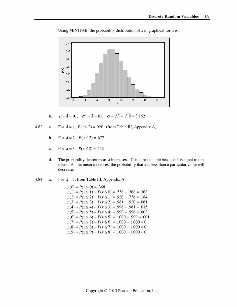
Using MINITAB, the probability distribution of x in graphical form is:
x
p(
x)
211815129630
0.14
0.12
0.10
0.08
0.06
0.04
0.02
0.00
b. 10μ λ= = , 2 10σ λ= = , 10 3.162σ λ= = = 4.82 a. For 1λ = , ( 2) .920P x ≤ = (from Table III, Appendix A) b. For 2λ = , ( 2) .677P x ≤ = c. For 3λ = , ( 2) .423P x ≤ = d. The probability decreases as λ increases. This is reasonable because λ is equal to the
mean. As the mean increases, the probability that x is less than a particular value will decrease.
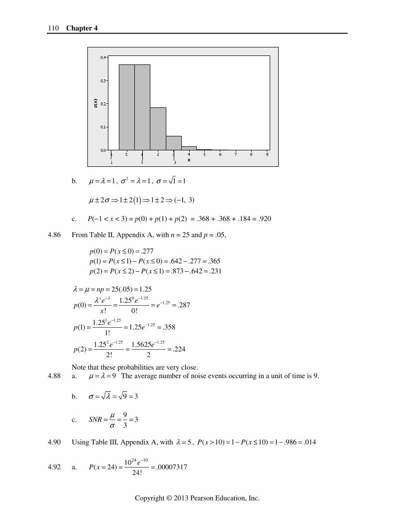
4.84 a. For 1λ = , from Table III, Appendix A. p(0) = P(x ≤ 0) = .368 p(1) = P(x ≤ 1) − P(x ≤ 0) = .736 − .368 = .368 p(2) = P(x ≤ 2) − P(x ≤ 1) = .920 − .736 = .184 p(3) = P(x ≤ 3) − P(x ≤ 2) = .981 − .920 = .061 p(4) = P(x ≤ 4) − P(x ≤ 3) = .996 − .981 = .015 p(5) = P(x ≤ 5) − P(x ≤ 4) = .999 − .996 = .003 p(6) = P(x ≤ 6) − P(x ≤ 5) = 1.000 − .999 = .001 p(7) = P(x ≤ 7) − P(x ≤ 6) = 1.000 − 1.000 = 0 p(8) = P(x ≤ 8) − P(x ≤ 7) = 1.000 − 1.000 = 0 p(9) = P(x ≤ 9) − P(x ≤ 8) = 1.000 − 1.000 = 0
110 Chapter 4
Copyright © 2013 Pearson Education, Inc.
x
p(
x)
9876543210-1
0.4
0.3
0.2
0.1
0.0
1-1 3
b. 1μ λ= = , 2 1σ λ= = , 1 1σ = = ( )2 1 2 1 1 2 ( 1, 3)μ σ± ⇒ ± ⇒ ± ⇒ − c. P(−1 < x < 3) = p(0) + p(1) + p(2) = .368 + .368 + .184 = .920 4.86 From Table II, Appendix A, with n = 25 and p = .05, (0) ( 0) .277p P x= ≤ = (1) ( 1) ( 0) .642 .277 .365p P x P x= ≤ − ≤ = − = (2) ( 2) ( 1) .873 .642 .231p P x P x= ≤ − ≤ = − = 25(.05) 1.25npλ μ= = = =
0 1.25
1.251.25(0) .287
! 0!
xe ep e
x
λλ − −−= = = =
1 1.25
1.251.25(1) 1.25 .358
1!
ep e
−−= = =
2 1.25 1.251.25 1.5625
(2) .2242! 2
e ep
− −
= = =
Note that these probabilities are very close. 4.88 a. 9μ λ= = The average number of noise events occurring in a unit of time is 9.
b. 9 3σ λ= = =
c. 9
33
SNRμσ
= = =
4.90 Using Table III, Appendix A, with 5λ = , ( 10) 1 ( 10) 1 .986 .014P x P x> = − ≤ = − =
4.92 a. 24 1010
( 24) .0000731724!
eP x
−
= = =
Discrete Random Variables 111
Copyright © 2013 Pearson Education, Inc.
b. 23 1010
( 23) .000175623!
eP x
−
= = =
c. The probability of “theft” is fairly close, rounded off to 4 decimal places (.00007317 ≈
.0001). However, the probability of “fire” is about twice the estimate of .0001 (.0001756 ≈ .0002).
4.94 a. 2 .25σ λ= =
b. .25μ λ= = , .25 .5σ = = ( )2 .25 2 .5 .25 1 ( .75, 1.25)μ σ± ⇒ ± ⇒ ± ⇒ −
0 1
( .75 1.25) ( 0) ( 1)0! 1!
e eP x P x P x
λ λλ λ− −
− < < = = + = = +
0 .25 1 .25.25 .25
.7788 .1947 .97350! 1!
e e− −
= + = + =
c. From part b, we found that the probability that the number of times the word “though”
appears once or fewer in 1,000 words is .9735. From this, we can find the probability that the word “though” appears more than once in 1,000 words as:
( 1) 1 ( 1) 1 .9735 .0265P x P x> = − ≤ = − = If Davey Crockett actually wrote the article, the probability of observing the word
“though” 2 times in the first 1,000 words is extremely unusual. We would conclude that Davey Crockett did not write the Texas narrative.
4.96 Using Table III, Appendix A, with .8λ = , ( 1) 1 ( 0) 1 .449 .551.P x P x≥ = − = = − = We
assumed that the number of flaws in a 4 meter length of wire follows a Poisson distribution. 4.98 The characteristics of a hypergeometric distribution are:
1. The experiment consists of randomly drawing n elements without replacement from a set of N elements, r of which are S’s (for Success) and (N – r) of which are F’s (for Failure).
2. The hypergeometric random variable x is the number of S’s in the draw of n elements. 4.100 Sampling with replacement means that once an experimental unit has been observed, it is
returned to the population before the next experimental unit is sampled. Thus, for each trial, each member of the population has a chance of being selected. The same experimental unit may be observed more than once.
Sampling without replacement means that once an experimental unit has been observed, it is
not returned to the population before the next experimental unit is observed. Thus, an experimental unit can only be observed once in each sample.
112 Chapter 4
Copyright © 2013 Pearson Education, Inc.
4.102 For N = 8, n = 3, and r = 5,
a.
5 8 5 5! 3!1 3 1 5(3)1!4! 2!1!( 1) .268
8!8 563!5!3
r N r
x n xP x
N
n
− −⎛ ⎞⎛ ⎞ ⎛ ⎞⎛ ⎞⎜ ⎟⎜ ⎟ ⎜ ⎟⎜ ⎟− −⎝ ⎠⎝ ⎠ ⎝ ⎠⎝ ⎠= = = = = =
⎛ ⎞ ⎛ ⎞⎜ ⎟ ⎜ ⎟⎝ ⎠ ⎝ ⎠
b.
5 8 5 5! 3!0 3 0 1(1)0!5! 3!0!( 0) .018
8!8 563!5!3
r N r
x n xP x
N
n
− −⎛ ⎞⎛ ⎞ ⎛ ⎞⎛ ⎞⎜ ⎟⎜ ⎟ ⎜ ⎟⎜ ⎟− −⎝ ⎠⎝ ⎠ ⎝ ⎠⎝ ⎠= = = = = =
⎛ ⎞ ⎛ ⎞⎜ ⎟ ⎜ ⎟⎝ ⎠ ⎝ ⎠
c.
5 8 5 5! 3!3 3 3 10(1)3!2! 0!3!( 3) .179
8!8 563!5!3
r N r
x n xP x
N
n
− −⎛ ⎞⎛ ⎞ ⎛ ⎞⎛ ⎞⎜ ⎟⎜ ⎟ ⎜ ⎟⎜ ⎟− −⎝ ⎠⎝ ⎠ ⎝ ⎠⎝ ⎠= = = = = =
⎛ ⎞ ⎛ ⎞⎜ ⎟ ⎜ ⎟⎝ ⎠ ⎝ ⎠
d. ( 4) 0P x ≥ = Since the sample size is only 3, there is no way to get 4 or more successes in only 3
trials. 4.104 From Exercise 4.103, the probability distribution of x in tabular form is:
x p(x) 2 .0303 .2424 .4555 .2426 .030
a. ( 1) 0P x = = b. ( 4) .455P x = = c. ( 4) ( 2) ( 3) ( 4) .030 .242 .455 .727P x P x P x P x≤ = = + = + = = + + = d. ( 5) ( 5) ( 6) .242 .030 .272P x P x P x≥ = = + = = + = e. ( 3) ( 2) .030P x P x< = = = f. ( 8) 0P x ≥ =
Discrete Random Variables 113
Copyright © 2013 Pearson Education, Inc.
4.106 With N = 10, n = 5, and r = 7, x can take on values 2, 3, 4, or 5.
a.
7 10 7 7! 3!2 5 2 21(1)2!5! 3!0!( 2) .083
10!10 2525!5!5
r N r
x n xP x
N
n
− −⎛ ⎞⎛ ⎞ ⎛ ⎞⎛ ⎞⎜ ⎟⎜ ⎟ ⎜ ⎟⎜ ⎟− −⎝ ⎠⎝ ⎠ ⎝ ⎠⎝ ⎠= = = = = =
⎛ ⎞ ⎛ ⎞⎜ ⎟ ⎜ ⎟⎝ ⎠ ⎝ ⎠
7 10 7 7! 3!3 5 3 35(3)3!4! 2!1!( 3) .417
10!10 2525!5!5
r N r
x n xP x
N
n
− −⎛ ⎞⎛ ⎞ ⎛ ⎞⎛ ⎞⎜ ⎟⎜ ⎟ ⎜ ⎟⎜ ⎟− −⎝ ⎠⎝ ⎠ ⎝ ⎠⎝ ⎠= = = = = =
⎛ ⎞ ⎛ ⎞⎜ ⎟ ⎜ ⎟⎝ ⎠ ⎝ ⎠
7 10 7 7! 3!4 5 4 35(3)4!3!1!2!( 4) .417
10!10 2525!5!5
r N r
x n xP x
N
n
− −⎛ ⎞⎛ ⎞ ⎛ ⎞⎛ ⎞⎜ ⎟⎜ ⎟ ⎜ ⎟⎜ ⎟− −⎝ ⎠⎝ ⎠ ⎝ ⎠⎝ ⎠= = = = = =
⎛ ⎞ ⎛ ⎞⎜ ⎟ ⎜ ⎟⎝ ⎠ ⎝ ⎠
7 10 7 7! 3!5 5 5 21(1)5!2! 0!3!( 5) .083
10!10 2525!5!5
r N r
x n xP x
N
n
− −⎛ ⎞⎛ ⎞ ⎛ ⎞⎛ ⎞⎜ ⎟⎜ ⎟ ⎜ ⎟⎜ ⎟− −⎝ ⎠⎝ ⎠ ⎝ ⎠⎝ ⎠= = = = = =
⎛ ⎞ ⎛ ⎞⎜ ⎟ ⎜ ⎟⎝ ⎠ ⎝ ⎠
The probability distribution of x in tabular form is:
x p(x) 2 .0833 .4174 .4175 .083
b. 5(7)
3.510
nr
Nμ = = =
22 2
( ) ( ) 7(10 7)5(10 5) 525.5833
( 1) 10 (10 1) 900
r N r n N n
N Nσ − − − −= = = =
− −
.5833 .764σ = =
114 Chapter 4
Copyright © 2013 Pearson Education, Inc.
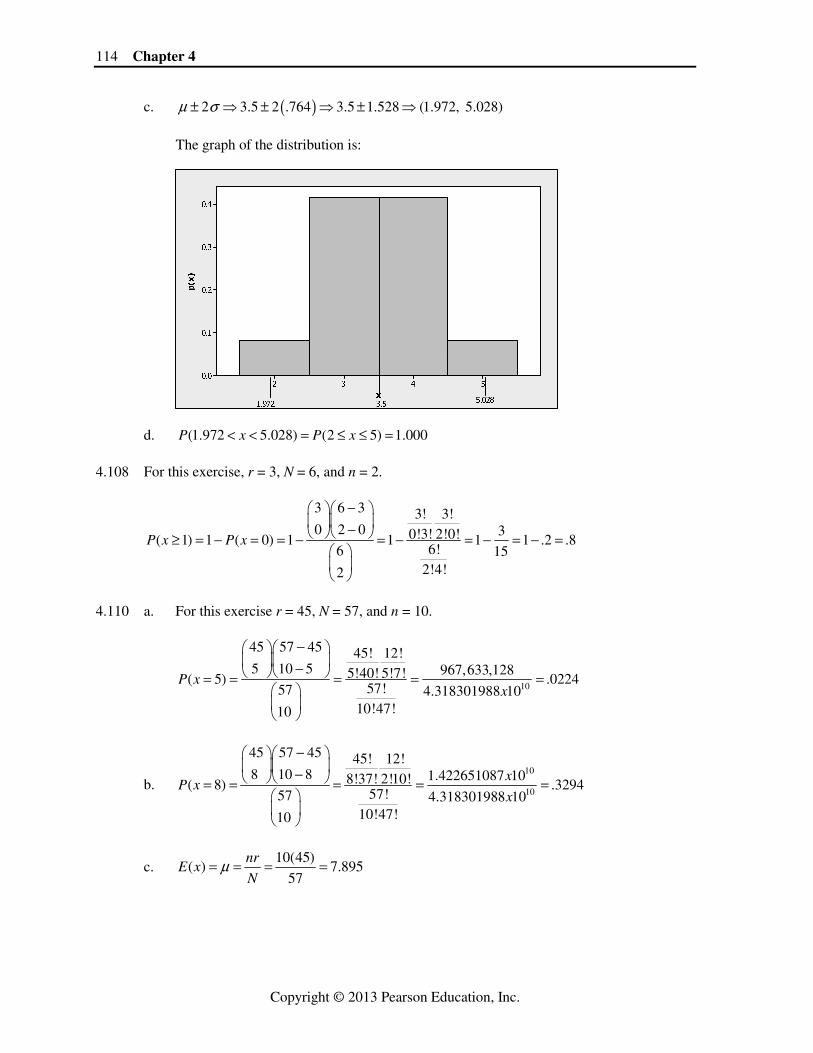
c. ( )2 3.5 2 .764 3.5 1.528 (1.972, 5.028)μ σ± ⇒ ± ⇒ ± ⇒
The graph of the distribution is:
x
p(
x)
5432
0.4
0.3
0.2
0.1
0.0
3.51.9725.028
d. (1.972 5.028) (2 5) 1.000P x P x< < = ≤ ≤ = 4.108 For this exercise, r = 3, N = 6, and n = 2.
3 6 3 3! 3!0 2 0 30!3! 2!0!( 1) 1 ( 0) 1 1 1 1 .2 .8
6!6 152!4!2
P x P x
−⎛ ⎞⎛ ⎞⎜ ⎟⎜ ⎟−⎝ ⎠⎝ ⎠≥ = − = = − = − = − = − =
⎛ ⎞⎜ ⎟⎝ ⎠
4.110 a. For this exercise r = 45, N = 57, and n = 10.
10
45 57 45 45! 12!5 10 5 967,633,1285!40! 5!7!( 5) .0224
57!57 4.318301988 1010!47!10
P xx
−⎛ ⎞⎛ ⎞⎜ ⎟⎜ ⎟−⎝ ⎠⎝ ⎠= = = = =
⎛ ⎞⎜ ⎟⎝ ⎠
b. 10
10
45 57 45 45! 12!8 10 8 1.422651087 108!37! 2!10!( 8) .3294
57!57 4.318301988 1010!47!10
xP x
x
−⎛ ⎞⎛ ⎞⎜ ⎟⎜ ⎟−⎝ ⎠⎝ ⎠= = = = =
⎛ ⎞⎜ ⎟⎝ ⎠
c. 10(45)
( ) 7.89557
nrE x
Nμ= = = =
Discrete Random Variables 115
Copyright © 2013 Pearson Education, Inc.
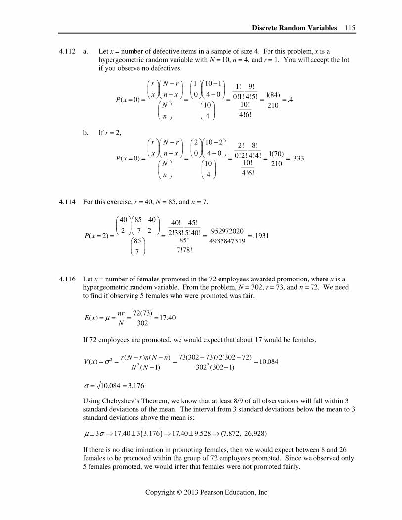
4.112 a. Let x = number of defective items in a sample of size 4. For this problem, x is a hypergeometric random variable with N = 10, n = 4, and r = 1. You will accept the lot if you observe no defectives.
1 10 1 1! 9!0 4 0 1(84)0!1! 4!5!( 0) .4
10!10 2104!6!4
r N r
x n xP x
N
n
− −⎛ ⎞⎛ ⎞ ⎛ ⎞⎛ ⎞⎜ ⎟⎜ ⎟ ⎜ ⎟⎜ ⎟− −⎝ ⎠⎝ ⎠ ⎝ ⎠⎝ ⎠= = = = = =
⎛ ⎞ ⎛ ⎞⎜ ⎟ ⎜ ⎟⎝ ⎠ ⎝ ⎠
b. If r = 2,
2 10 2 2! 8!0 4 0 1(70)0!2! 4!4!( 0) .333
10!10 2104!6!4
r N r
x n xP x
N
n
− −⎛ ⎞⎛ ⎞ ⎛ ⎞⎛ ⎞⎜ ⎟⎜ ⎟ ⎜ ⎟⎜ ⎟− −⎝ ⎠⎝ ⎠ ⎝ ⎠⎝ ⎠= = = = = =
⎛ ⎞ ⎛ ⎞⎜ ⎟ ⎜ ⎟⎝ ⎠ ⎝ ⎠
4.114 For this exercise, r = 40, N = 85, and n = 7.
40 85 40 40! 45!2 7 2 9529720202!38! 5!40!( 2) .1931
85!85 49358473197!78!7
P x
−⎛ ⎞⎛ ⎞⎜ ⎟⎜ ⎟−⎝ ⎠⎝ ⎠= = = = =
⎛ ⎞⎜ ⎟⎝ ⎠
4.116 Let x = number of females promoted in the 72 employees awarded promotion, where x is a
hypergeometric random variable. From the problem, N = 302, r = 73, and n = 72. We need to find if observing 5 females who were promoted was fair.
72(73)
( ) 17.40302
nrE x
Nμ= = = =
If 72 employees are promoted, we would expect that about 17 would be females.
22 2
( ) ( ) 73(302 73)72(302 72)( ) 10.084
( 1) 302 (302 1)
r N r n N nV x
N Nσ − − − −= = = =
− −
10.084 3.176σ = =
Using Chebyshev’s Theorem, we know that at least 8/9 of all observations will fall within 3 standard deviations of the mean. The interval from 3 standard deviations below the mean to 3 standard deviations above the mean is:
( )3 17.40 3 3.176 17.40 9.528 (7.872, 26.928)μ σ± ⇒ ± ⇒ ± ⇒
If there is no discrimination in promoting females, then we would expect between 8 and 26 females to be promoted within the group of 72 employees promoted. Since we observed only
5 females promoted, we would infer that females were not promoted fairly.

116 Chapter 4
Copyright © 2013 Pearson Education, Inc.
4.118 a. The length of time that an exercise physiologist's program takes to elevate her client's heart rate to 140 beats per minute is measured on an interval and thus, is continuous.
b. The number of crimes committed on a college campus per year is a whole number such
as 0, 1, 2, etc. This variable is discrete. c. The number of square feet of vacant office space in a large city is a measurement of
area and is measured on an interval. Thus, this variable is continuous. d. The number of voters who favor a new tax proposal is a whole number such as 0, 1, 2,
etc. This variable is discrete. 4.120 a. This experiment consists of 100 trials. Each trial results in one of two outcomes: chip
is defective or not defective. If the number of chips produced in one hour is much larger than 100, then we can assume the probability of a defective chip is the same on each trial and that the trials are independent. Thus, x is a binomial. If, however, the number of chips produced in an hour is not much larger than 100, the trials would not be independent. Then x would not be a binomial random variable.
b. This experiment consists of two trials. Each trial results in one of two outcomes:
applicant qualified or not qualified. However, the trials are not independent. The probability of selecting a qualified applicant on the first trial is 3 out of 5. The probability of selecting a qualified applicant on the second trial depends on what happened on the first trial. Thus, x is not a binomial random variable. It is a hypergeometric random variable.
c. The number of trials is not a specified number in this experiment, thus x is not a
binomial random variable. In this experiment, x is counting the number of calls received in a specific time frame. Thus, x is a Poisson random variable.
d. The number of trials in this experiment is 1000. Each trial can result in one of two
outcomes: favor state income tax or not favor state income tax. Since 1000 is small compared to the number of registered voters in Florida, the probability of selecting a voter in favor of the state income tax is the same from trial to trial, and the trials are independent of each other. Thus, x is a binomial random variable.
4.122 a.
3 8 3 3! 5!2 5 2 3(10)2!1! 3!2!( 2) .536
8!8 565!3!5
r N r
x n xP x
N
n
− −⎛ ⎞⎛ ⎞ ⎛ ⎞⎛ ⎞⎜ ⎟⎜ ⎟ ⎜ ⎟⎜ ⎟− −⎝ ⎠⎝ ⎠ ⎝ ⎠⎝ ⎠= = = = = =
⎛ ⎞ ⎛ ⎞⎜ ⎟ ⎜ ⎟⎝ ⎠ ⎝ ⎠
b.
2 6 2 2! 4!2 2 2 1(1)2!0! 0!4!( 2) .067
6!6 152!4!2
r N r
x n xP x
N
n
− −⎛ ⎞⎛ ⎞ ⎛ ⎞⎛ ⎞⎜ ⎟⎜ ⎟ ⎜ ⎟⎜ ⎟− −⎝ ⎠⎝ ⎠ ⎝ ⎠⎝ ⎠= = = = = =
⎛ ⎞ ⎛ ⎞⎜ ⎟ ⎜ ⎟⎝ ⎠ ⎝ ⎠
Discrete Random Variables 117
Copyright © 2013 Pearson Education, Inc.
c.
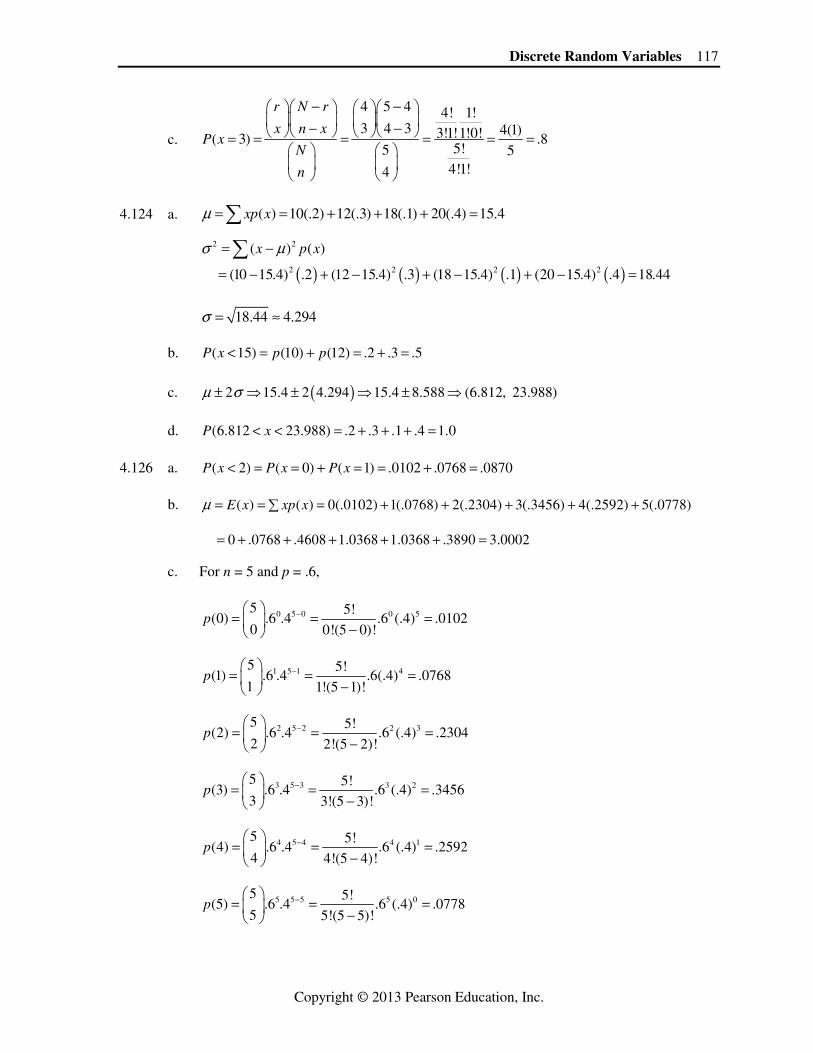
4 5 4 4! 1!3 4 3 4(1)3!1!1!0!( 3) .8
5!5 54!1!4
r N r
x n xP x
N
n
− −⎛ ⎞⎛ ⎞ ⎛ ⎞⎛ ⎞⎜ ⎟⎜ ⎟ ⎜ ⎟⎜ ⎟− −⎝ ⎠⎝ ⎠ ⎝ ⎠⎝ ⎠= = = = = =
⎛ ⎞ ⎛ ⎞⎜ ⎟ ⎜ ⎟⎝ ⎠ ⎝ ⎠
4.124 a. ( ) 10(.2) 12(.3) 18(.1) 20(.4) 15.4xp xμ = = + + + =∑
( ) ( ) ( ) ( )
2 2
2 2 2 2
( ) ( )
(10 15.4) .2 (12 15.4) .3 (18 15.4) .1 (20 15.4) .4 18.44
x p xσ μ= −
= − + − + − + − =∑
18.44 4.294σ = ≈ b. ( 15) (10) (12) .2 .3 .5P x p p< = + = + = c. ( )2 15.4 2 4.294 15.4 8.588 (6.812, 23.988)μ σ± ⇒ ± ⇒ ± ⇒
d. (6.812 23.988) .2 .3 .1 .4 1.0P x< < = + + + = 4.126 a. ( 2) ( 0) ( 1) .0102 .0768 .0870P x P x P x< = = + = = + = b. ( ) ( ) 0(.0102) 1(.0768) 2(.2304) 3(.3456) 4(.2592) 5(.0778)E x xp xμ = = = + + + + +∑
0 .0768 .4608 1.0368 1.0368 .3890 3.0002= + + + + + =
c. For n = 5 and p = .6,
0 5 0 0 55 5!(0) .6 .4 .6 (.4) .0102
0 0!(5 0)!p −⎛ ⎞
= = =⎜ ⎟ −⎝ ⎠
1 5 1 45 5!(1) .6 .4 .6(.4) .0768
1 1!(5 1)!p −⎛ ⎞
= = =⎜ ⎟ −⎝ ⎠
2 5 2 2 35 5!(2) .6 .4 .6 (.4) .2304
2 2!(5 2)!p −⎛ ⎞
= = =⎜ ⎟ −⎝ ⎠
3 5 3 3 25 5!(3) .6 .4 .6 (.4) .3456
3 3!(5 3)!p −⎛ ⎞
= = =⎜ ⎟ −⎝ ⎠
4 5 4 4 15 5!(4) .6 .4 .6 (.4) .2592
4 4!(5 4)!p −⎛ ⎞
= = =⎜ ⎟ −⎝ ⎠
5 5 5 5 05 5!(5) .6 .4 .6 (.4) .0778
5 5!(5 5)!p −⎛ ⎞
= = =⎜ ⎟ −⎝ ⎠
118 Chapter 4
Copyright © 2013 Pearson Education, Inc.
Since all the probabilities are the same as in the table, x is a binomial random variable with n = 5 and p = .6.
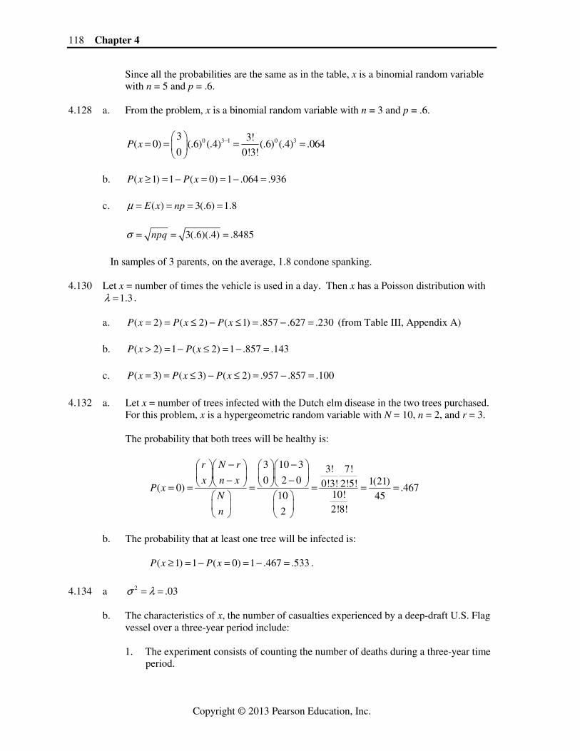
4.128 a. From the problem, x is a binomial random variable with n = 3 and p = .6.
0 3 1 0 33 3!( 0) (.6) (.4) (.6) (.4) .064
0 0!3!P x −⎛ ⎞
= = = =⎜ ⎟⎝ ⎠
b. ( 1) 1 ( 0) 1 .064 .936P x P x≥ = − = = − = c. ( ) 3(.6) 1.8E x npμ = = = = 3(.6)(.4) .8485npqσ = = =
In samples of 3 parents, on the average, 1.8 condone spanking. 4.130 Let x = number of times the vehicle is used in a day. Then x has a Poisson distribution with
1.3λ = . a. ( 2) ( 2) ( 1) .857 .627 .230P x P x P x= = ≤ − ≤ = − = (from Table III, Appendix A) b. ( 2) 1 ( 2) 1 .857 .143P x P x> = − ≤ = − = c. ( 3) ( 3) ( 2) .957 .857 .100P x P x P x= = ≤ − ≤ = − =
4.132 a. Let x = number of trees infected with the Dutch elm disease in the two trees purchased.
For this problem, x is a hypergeometric random variable with N = 10, n = 2, and r = 3. The probability that both trees will be healthy is:
3 10 3 3! 7!0 2 0 1(21)0!3! 2!5!( 0) .467
10!10 452!8!2
r N r
x n xP x
N
n
− −⎛ ⎞⎛ ⎞ ⎛ ⎞⎛ ⎞⎜ ⎟⎜ ⎟ ⎜ ⎟⎜ ⎟− −⎝ ⎠⎝ ⎠ ⎝ ⎠⎝ ⎠= = = = = =
⎛ ⎞ ⎛ ⎞⎜ ⎟ ⎜ ⎟⎝ ⎠ ⎝ ⎠
b. The probability that at least one tree will be infected is: ( 1) 1 ( 0) 1 .467 .533P x P x≥ = − = = − = . 4.134 a 2 .03σ λ= = b. The characteristics of x, the number of casualties experienced by a deep-draft U.S. Flag
vessel over a three-year period include: 1. The experiment consists of counting the number of deaths during a three-year time
period.
Discrete Random Variables 119
Copyright © 2013 Pearson Education, Inc.
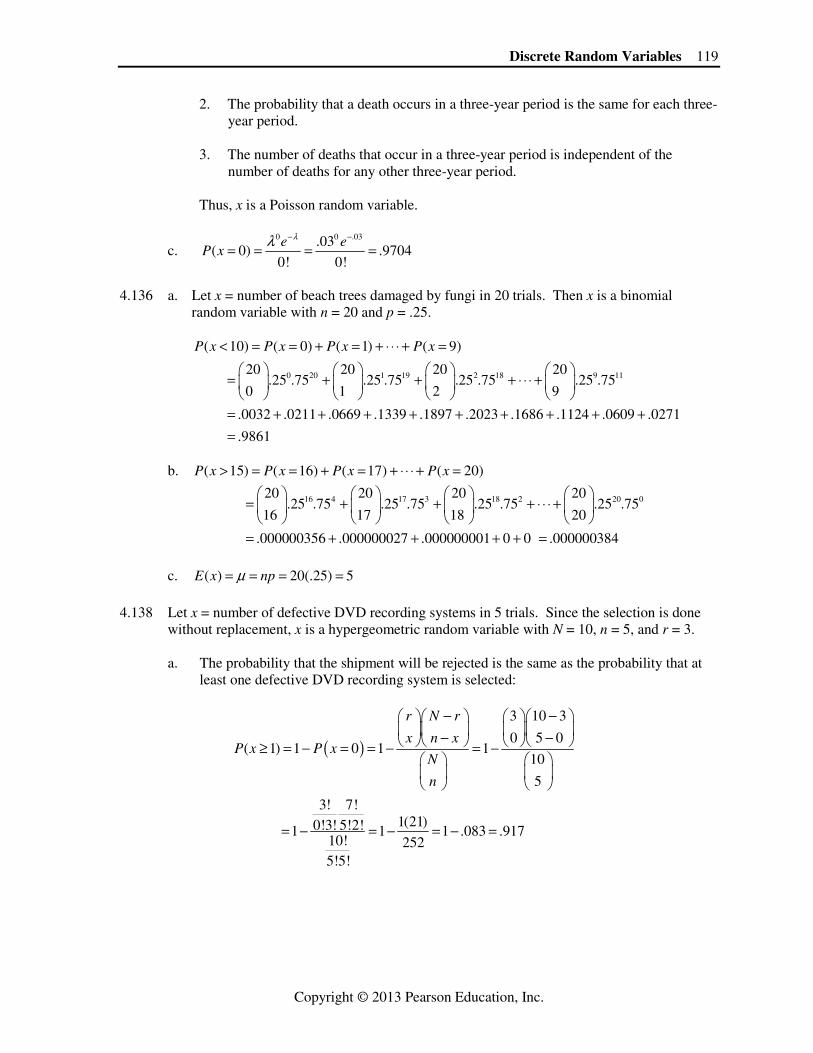
2. The probability that a death occurs in a three-year period is the same for each three-year period.
3. The number of deaths that occur in a three-year period is independent of the
number of deaths for any other three-year period. Thus, x is a Poisson random variable.
c. 0 0 .03.03
( 0) .97040! 0!
e eP x
λλ − −
= = = =
4.136 a. Let x = number of beach trees damaged by fungi in 20 trials. Then x is a binomial
random variable with n = 20 and p = .25.
0 20 1 19 2 18 9 11
( 10) ( 0) ( 1) ( 9)
20 20 20 20 .25 .75 .25 .75 .25 .75 .25 .75
0 1 2 9
.0032 .0211 .0669 .1339 .1897 .2023 .1686 .1124 .0609 .0271
.98
P x P x P x P x< = = + = + ⋅ ⋅ ⋅ + =
⎛ ⎞ ⎛ ⎞ ⎛ ⎞ ⎛ ⎞= + + + ⋅ ⋅ ⋅ +⎜ ⎟ ⎜ ⎟ ⎜ ⎟ ⎜ ⎟⎝ ⎠ ⎝ ⎠ ⎝ ⎠ ⎝ ⎠
= + + + + + + + + += 61
b. ( 15) ( 16) ( 17) ( 20)P x P x P x P x> = = + = + ⋅⋅ ⋅ + =
16 4 17 3 18 2 20 020 20 20 20
.25 .75 .25 .75 .25 .75 .25 .7516 17 18 20
.000000356 .000000027 .000000001 0 0 .000000384
⎛ ⎞ ⎛ ⎞ ⎛ ⎞ ⎛ ⎞= + + + ⋅ ⋅ ⋅ +⎜ ⎟ ⎜ ⎟ ⎜ ⎟ ⎜ ⎟⎝ ⎠ ⎝ ⎠ ⎝ ⎠ ⎝ ⎠
= + + + + =
c. ( ) 20(.25) 5E x npμ= = = = 4.138 Let x = number of defective DVD recording systems in 5 trials. Since the selection is done
without replacement, x is a hypergeometric random variable with N = 10, n = 5, and r = 3. a. The probability that the shipment will be rejected is the same as the probability that at
least one defective DVD recording system is selected:
( )
3 10 3
0 5 0( 1) 1 0 1 1
10
5
3! 7!1(21)0!3! 5!2!1 1 1 .083 .917
10! 2525!5!
r N r
x n xP x P x
N
n
− −⎛ ⎞⎛ ⎞ ⎛ ⎞⎛ ⎞⎜ ⎟⎜ ⎟ ⎜ ⎟⎜ ⎟− −⎝ ⎠⎝ ⎠ ⎝ ⎠⎝ ⎠≥ = − = = − = −
⎛ ⎞ ⎛ ⎞⎜ ⎟ ⎜ ⎟⎝ ⎠ ⎝ ⎠
= − = − = − =
120 Chapter 4
Copyright © 2013 Pearson Education, Inc.
b. If 6 DVD recording systems are selected, the shipment will be accepted if none of the systems are defective:
3 10 3 3! 7!0 6 0 1(7)0!3! 6!1!( 0) .033
10!10 2106!4!6
r N r
x n xP x
N
n
− −⎛ ⎞⎛ ⎞ ⎛ ⎞⎛ ⎞⎜ ⎟⎜ ⎟ ⎜ ⎟⎜ ⎟− −⎝ ⎠⎝ ⎠ ⎝ ⎠⎝ ⎠= = = = = =
⎛ ⎞ ⎛ ⎞⎜ ⎟ ⎜ ⎟⎝ ⎠ ⎝ ⎠
4.140 Let x = number of British bird species sampled that inhabit a butterfly hotspot in 4 trials.
Because the sampling is done without replacement, x is a hypergeometric random variable with N = 10, n = 4, and r = 7.
a.
7 10 7 7! 3!2 4 2 21(3)2!5! 2!1!( 2) .3
10!10 2104!6!4
r N r
x n xP x
N
n
− −⎛ ⎞⎛ ⎞ ⎛ ⎞⎛ ⎞⎜ ⎟⎜ ⎟ ⎜ ⎟⎜ ⎟− −⎝ ⎠⎝ ⎠ ⎝ ⎠⎝ ⎠= = = = = =
⎛ ⎞ ⎛ ⎞⎜ ⎟ ⎜ ⎟⎝ ⎠ ⎝ ⎠
b. ( 1) 1P x ≥ = because the only values x can take on are 1, 2, 3, or 4. 4.142 a. Let x = number of democratic regimes that allow a free press in 50 trials. For this
problem, p = .8. ( ) 50(.8) 40E x npμ = = = = We would expect 40 democratic regimes out of the 50 to have a free press.
(1 ) 50(.8)(.2) 2.828np pσ = − = =
We would expect most observations to fall within 2 standard deviations of the mean: ( )2 40 2 2.828 40 5.656 (34.344, 45.656)μ σ± ⇒ ± ⇒ ± ⇒
We would expect to see anywhere between 35 and 45 democratic regimes to have a free
press out of a sample of 50. b. Let x = number of non-democratic regimes that allow a free press in 50 trials. For this
problem, p = .1. ( ) 50(.1) 5E x npμ = = = = We would expect 5 non-democratic regimes out of the 50 to have a free press. (1 ) 50(.1)(.9) 2.121np pσ = − = =

Discrete Random Variables 121
Copyright © 2013 Pearson Education, Inc.
We would expect most observations to fall within 2 standard deviations of the mean: ( )2 5 2 2.121 5 4.242 (0.758, 9.242)μ σ± ⇒ ± ⇒ ± ⇒
We would expect to see anywhere between 1 to 9 non-democratic regimes to have a free
press out of a sample of 50. 4.144 a. ( 3) .010P x ≤ = using Table III, Appendix A with 10λ = . b. Yes. The probability of observing 3 or fewer crimes in a year if the mean is still 10 is
extremely small. This is evidence that the Crime Watch group has been effective in this neighborhood.
4.146 a. Let x = number of failures in 10 trials. Then x is a binomial random variable with n =
20 and p = .10. ( 1) .392P x ≤ = using Table II, Appendix A, with n = 20 and p = .10. b. Level of confidence = 1 ( 1) 1 .392 .608P x− ≤ = − = . This is a rather low level of
confidence. If this “one shot” device was life threatening, a level of confidence of only .608 is rather small.
c. Level of confidence = 1 ( )P x K− ≤ . If we keep K = 1 from above, but change n to 25 instead of 20, we get: Level of confidence = 1 ( 1) 1 .271 .729P x− ≤ = − = . If we keep n = 20 but decrease K from 1 to 0, we get: Level of confidence = 1 ( 0) 1 .122 .878P x− ≤ = − = . In both of these cases, the level of confidence has increased for the original value.
d. We want level of confidence to be greater than or equal to .95. Thus, 1 ( ) .95P x K− ≤ ≥ or ( ) .05P x K≤ ≤ With p = .10 and k = 0,
0 0( 0) .05 .1 .9 .05 .9 .05 ln(.9) ln(.05)
0
( .105360515) ( .2995732274) 28.4
n nnP x n
n n
−⎛ ⎞= ≤ ⇒ ≤ ⇒ ≤ ⇒ ≤⎜ ⎟
⎝ ⎠⇒ − ≤ − ⇒ ≥
Thus if k = 0, n would have to be 29 or more. With p = .10 and k = 1,
122 Chapter 4
Copyright © 2013 Pearson Education, Inc.
0 0 1 1 1( 1) .05 .1 .9 .1 .9 .05 .9 (.1)(.9) .050 1
n n n nn nP x n− − −⎛ ⎞ ⎛ ⎞
≤ ≤ ⇒ + ≤ ⇒ + ≤⎜ ⎟ ⎜ ⎟⎝ ⎠ ⎝ ⎠
Through trial and error, n would have to be greater than or equal to 46. Thus if k = 1, n would have to be 46 or more. 4.148 Let x = number of disasters in 25 trials. If NASA’s assessment is correct, then x is a binomial
random variable with n = 25 and p = 1 / 60,000 = .00001667. If the Air Force’s assessment is correct, then x is a binomial random variable with n = 25 and p = 1 / 35 = .02857.
If NASA’s assessment is correct, then the probability of no disasters in 25 missions would be:
0 2525( 0) (1/ 60,000) (59,999 / 60,000) .9996
0P x
⎛ ⎞= = =⎜ ⎟
⎝ ⎠
Thus, the probability of at least one disaster would be ( 1) 1 ( 0) 1 .9996 .0004P x P x≥ = − = = − = If the Air Force’s assessment is correct, then the probability of no disasters in 25 missions would be:
0 2525( 0) (1/ 35) (34 / 35) .4845
0P x
⎛ ⎞= = =⎜ ⎟
⎝ ⎠
Thus, the probability of at least one disaster would be ( 1) 1 ( 0) 1 .4845 .5155P x P x≥ = − = = − = One disaster actually did occur. If NASA’s assessment was correct, it would be almost impossible for at least one disaster to occur in 25 trials. If the Air Force’s assessment was correct, one disaster in 25 trials would not be an unusual event. Thus, the Air Force’s assessment appears to be appropriate.
Related Documents