Digital image processing

Seminar Report on

Digital Image Processing

Submitted by

Trishna Pattanaik

< Regd. No.: 1301229183 >

Project Report submitted in partial fulfillment of the

requirements for the award of the degree of

B.Tech. in Computer Science & Engineering under

Biju Pattnaik University of Technology (BPUT)

2016-2017

Under the Guidance of

Surajit Mohanty

HOD Dept. of CSE

Department of Computer Science & Engineering

DRIEMS Tangi, Cuttack-745022

CERTIFICATE

This is to certify that the project Digital Image Processing presented

by Trishna Pattanaik bearing Registration No. 1301229183 of

Department of Computer Science and Engineering in DRIEMS,

Cuttack has been completed successfully.

This is in partial fulfillment of the requirements of Bachelor Degree in

Computer Science and Engineering under Biju Pattnaik University of

Technology, Rourkela, Orissa.

I wish her success in all future endeavors.

Prof. Surajit Mohanty Prof. Surajit Mohanty Head of the Department Guide Computer Science & Engineering Computer Science & Engineering

Date: 19th March 2016 Date: 19th March 2016

ACKNOWLEDGEMENT

I express my sincere gratitude to Prof. Surajit Mohanty of Computer

Science and Engineering for giving me an opportunity to accomplish

seminar on the project. Without his active support and guidance, this

seminar would not have been successfully completed.

Trishna Pattanaik

Department of Computer Science & Engineering Regd.No.- 1301229183

Digital Image Processing

ABSTRACT

Digital image processing (dip) methods stems for two principal application areas: improvement of pictorial information for human interpretation and processing of image data for storage, transmission and representation for autonomous machine perception. Thus, the objectives of the topic are: to define the scope of the field, to give a historical perspective of the origins of this field, to give the idea of the state of the art in dip by examining some of the principal areas in which it is applied, to discuss briefly the principal approaches used in dip and to give an overview of the components contained in a typical general-purpose image processing system. Signature of the Guide Signature of the Student

Name : Prof. Surajit Mohanty Name : Trishna Pattanaik

Date : 19th March 2016 Regn. No : 1301229183

Semester : 6th

Branch : CSE

Section : C

Date : 19th March 2016

TABLE OF CONTENTS

CHAPTER NO. TITLE PAGE NO.

CERTIFICATE i

ACKNOWLEDGEMENT ii

ABSTRACT iii

LIST OF FIGURES v

1. INTRODUCTION 1

1.1 What is digital image processing? 1

1.2 The origins of Digital Image Processing 1

1.3 Fundamental steps for Digital Image Processing 2

2. DIGITAL IMAGE FUNDAMENTALS 4

2.1 Image Acquisition 4

2.2 Image Enhancement 5

2.3 Image Restoration 6

3. COLOR IMAGE PROCESSING 13

5.1 Pseudocolor Image Processing 13

5.2 Full-color Image Processing 13

4. MULTIRESOLUTION & MORPHOLOGICAL 14

IMAGE PROCESSING

4.1 Wavelets & Multiresolution Processing 14

4.2 Morphological Image Processing 15

5. IMAGE SEGMENTATION 16

6. COMPRESSION & REPRESENTATION 17

6.1 Image Compression 17

6.2 Representation & Description 18

6.3 Object Recognition 20

7. FIELDS OF APPLICATION 21

CONCLUSION 23

REFERENCES 24

LIST OF FIGURES

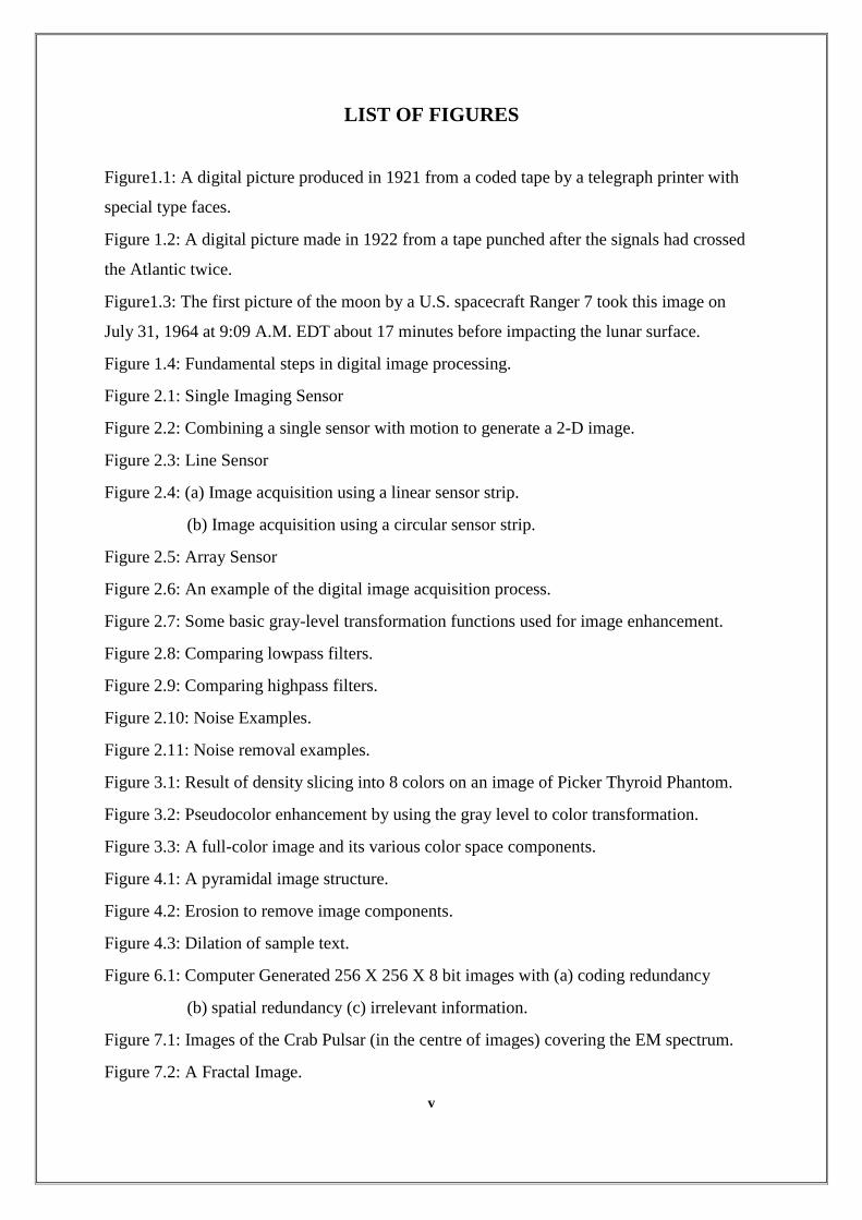
Figure1.1: A digital picture produced in 1921 from a coded tape by a telegraph printer with

special type faces.

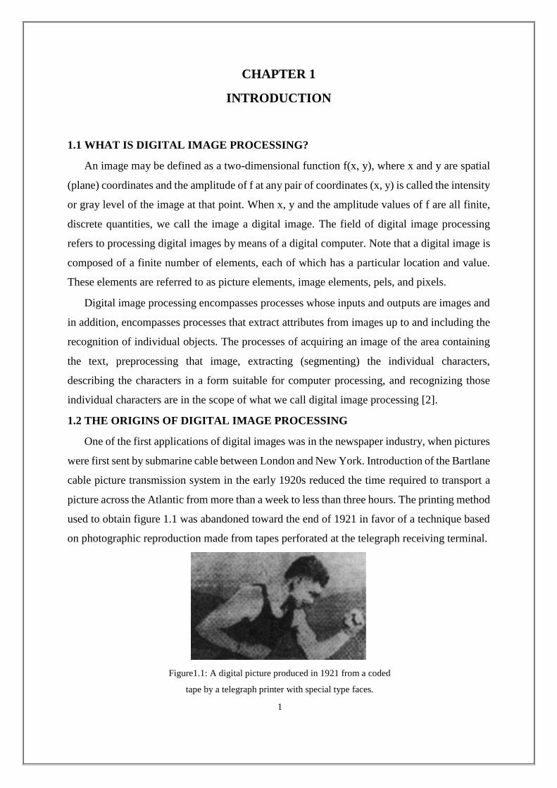
Figure 1.2: A digital picture made in 1922 from a tape punched after the signals had crossed

the Atlantic twice.

Figure1.3: The first picture of the moon by a U.S. spacecraft Ranger 7 took this image on

July 31, 1964 at 9:09 A.M. EDT about 17 minutes before impacting the lunar surface.

Figure 1.4: Fundamental steps in digital image processing.

Figure 2.1: Single Imaging Sensor

Figure 2.2: Combining a single sensor with motion to generate a 2-D image.

Figure 2.3: Line Sensor

Figure 2.4: (a) Image acquisition using a linear sensor strip.

(b) Image acquisition using a circular sensor strip.

Figure 2.5: Array Sensor

Figure 2.6: An example of the digital image acquisition process.

Figure 2.7: Some basic gray-level transformation functions used for image enhancement.

Figure 2.8: Comparing lowpass filters.

Figure 2.9: Comparing highpass filters.

Figure 2.10: Noise Examples.

Figure 2.11: Noise removal examples.

Figure 3.1: Result of density slicing into 8 colors on an image of Picker Thyroid Phantom.

Figure 3.2: Pseudocolor enhancement by using the gray level to color transformation.

Figure 3.3: A full-color image and its various color space components.

Figure 4.1: A pyramidal image structure.

Figure 4.2: Erosion to remove image components.

Figure 4.3: Dilation of sample text.

Figure 6.1: Computer Generated 256 X 256 X 8 bit images with (a) coding redundancy

(b) spatial redundancy (c) irrelevant information.

Figure 7.1: Images of the Crab Pulsar (in the centre of images) covering the EM spectrum.

Figure 7.2: A Fractal Image.

v

CHAPTER 1

INTRODUCTION

1.1 WHAT IS DIGITAL IMAGE PROCESSING?

An image may be defined as a two-dimensional function f(x, y), where x and y are spatial

(plane) coordinates and the amplitude of f at any pair of coordinates (x, y) is called the intensity

or gray level of the image at that point. When x, y and the amplitude values of f are all finite,

discrete quantities, we call the image a digital image. The field of digital image processing

refers to processing digital images by means of a digital computer. Note that a digital image is

composed of a finite number of elements, each of which has a particular location and value.

These elements are referred to as picture elements, image elements, pels, and pixels.

Digital image processing encompasses processes whose inputs and outputs are images and

in addition, encompasses processes that extract attributes from images up to and including the

recognition of individual objects. The processes of acquiring an image of the area containing

the text, preprocessing that image, extracting (segmenting) the individual characters,

describing the characters in a form suitable for computer processing, and recognizing those

individual characters are in the scope of what we call digital image processing [2].

1.2 THE ORIGINS OF DIGITAL IMAGE PROCESSING

One of the first applications of digital images was in the newspaper industry, when pictures

were first sent by submarine cable between London and New York. Introduction of the Bartlane

cable picture transmission system in the early 1920s reduced the time required to transport a

picture across the Atlantic from more than a week to less than three hours. The printing method

used to obtain figure 1.1 was abandoned toward the end of 1921 in favor of a technique based

on photographic reproduction made from tapes perforated at the telegraph receiving terminal.

Figure1.1: A digital picture produced in 1921 from a coded

tape by a telegraph printer with special type faces.

1

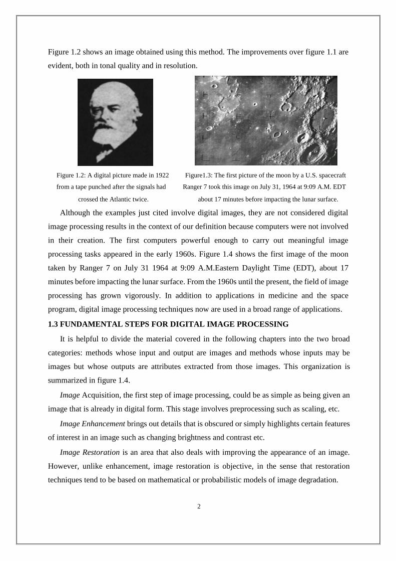
Figure 1.2 shows an image obtained using this method. The improvements over figure 1.1 are

evident, both in tonal quality and in resolution.

Figure 1.2: A digital picture made in 1922 Figure1.3: The first picture of the moon by a U.S. spacecraft

from a tape punched after the signals had Ranger 7 took this image on July 31, 1964 at 9:09 A.M. EDT

crossed the Atlantic twice. about 17 minutes before impacting the lunar surface.

Although the examples just cited involve digital images, they are not considered digital

image processing results in the context of our definition because computers were not involved

in their creation. The first computers powerful enough to carry out meaningful image

processing tasks appeared in the early 1960s. Figure 1.4 shows the first image of the moon

taken by Ranger 7 on July 31 1964 at 9:09 A.M.Eastern Daylight Time (EDT), about 17

minutes before impacting the lunar surface. From the 1960s until the present, the field of image

processing has grown vigorously. In addition to applications in medicine and the space

program, digital image processing techniques now are used in a broad range of applications.

1.3 FUNDAMENTAL STEPS FOR DIGITAL IMAGE PROCESSING

It is helpful to divide the material covered in the following chapters into the two broad

categories: methods whose input and output are images and methods whose inputs may be

images but whose outputs are attributes extracted from those images. This organization is

summarized in figure 1.4.

Image Acquisition, the first step of image processing, could be as simple as being given an

image that is already in digital form. This stage involves preprocessing such as scaling, etc.

Image Enhancement brings out details that is obscured or simply highlights certain features

of interest in an image such as changing brightness and contrast etc.

Image Restoration is an area that also deals with improving the appearance of an image.

However, unlike enhancement, image restoration is objective, in the sense that restoration

techniques tend to be based on mathematical or probabilistic models of image degradation.

2

Figure 1.4: Fundamental steps in digital image processing.

Color Image Processing is an area that has been gaining its importance because of the

significant increase in the use of digital images over the Internet. This may include color

modeling and processing in a digital domain etc.

Wavelets are foundation for representing images in various degrees of resolution. Images

subdivision successively into smaller regions for data compression and for pyramidal

representation.

Compression deals with techniques for reducing the storage required to save an image or

the bandwidth to transmit it. Particularly in the uses of internet it is very much necessary to

compress data.

Morphological Processing deals with tools for extracting image components that are useful

in the representation and description of shape.

Segmentation procedures partition an image into its constituent parts or objects. A rugged

segmentation procedure brings the process a long way toward successful solution of imaging

problems that require objects to be identified individually.

Representation and Description always follows the output of a segmentation stage, which

usually is raw pixel data, constituting either the boundary of a region itself. Choosing a

representation is only part of the solution for transforming raw data into a suitable for

subsequent computer processing. Description deals with extracting attributes that result in some

quantitative information of interest or are basic for differentiating one class of objects from

another.

Object Recognition is the process that assigns a label such as vehicle to an object based on

its descriptors.

3

CHAPTER 2

DIGITAL IMAGE FUNDAMENTALS

2.1 IMAGE ACQUISITION

The types of images in which we are interested are generated by the combination of an

“illumination” source and the reflection or absorption of energy from that source by the

elements of the “scene” being imaged. Thus, three principal sensor arrangements used to

transform illumination energy into digital images: single imaging sensor, line sensor or sensor

strips and array sensor [3].

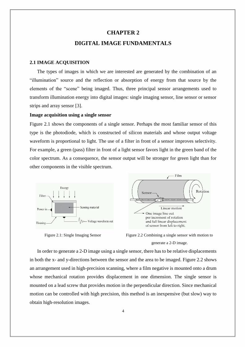
Image acquisition using a single sensor

Figure 2.1 shows the components of a single sensor. Perhaps the most familiar sensor of this

type is the photodiode, which is constructed of silicon materials and whose output voltage

waveform is proportional to light. The use of a filter in front of a sensor improves selectivity.

For example, a green (pass) filter in front of a light sensor favors light in the green band of the

color spectrum. As a consequence, the sensor output will be stronger for green light than for

other components in the visible spectrum.

Figure 2.1: Single Imaging Sensor Figure 2.2 Combining a single sensor with motion to

generate a 2-D image.

In order to generate a 2-D image using a single sensor, there has to be relative displacements

in both the x- and y-directions between the sensor and the area to be imaged. Figure 2.2 shows

an arrangement used in high-precision scanning, where a film negative is mounted onto a drum

whose mechanical rotation provides displacement in one dimension. The single sensor is

mounted on a lead screw that provides motion in the perpendicular direction. Since mechanical

motion can be controlled with high precision, this method is an inexpensive (but slow) way to

obtain high-resolution images.

4

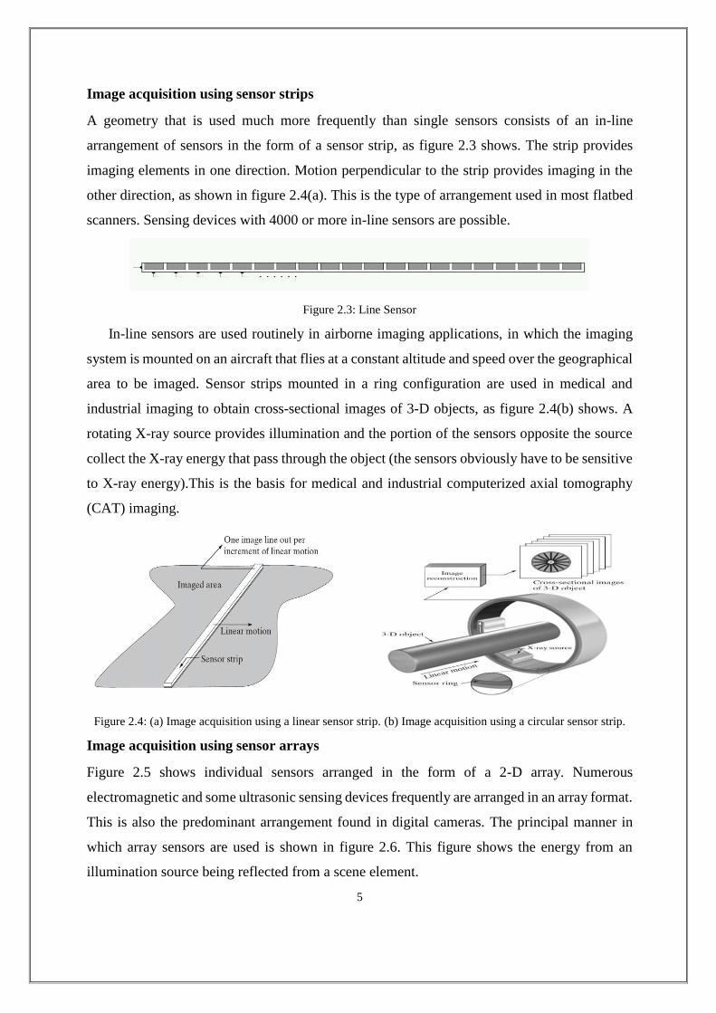
Image acquisition using sensor strips

A geometry that is used much more frequently than single sensors consists of an in-line

arrangement of sensors in the form of a sensor strip, as figure 2.3 shows. The strip provides

imaging elements in one direction. Motion perpendicular to the strip provides imaging in the

other direction, as shown in figure 2.4(a). This is the type of arrangement used in most flatbed

scanners. Sensing devices with 4000 or more in-line sensors are possible.

Figure 2.3: Line Sensor

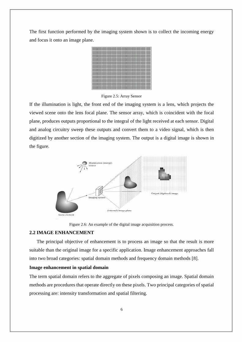
In-line sensors are used routinely in airborne imaging applications, in which the imaging

system is mounted on an aircraft that flies at a constant altitude and speed over the geographical

area to be imaged. Sensor strips mounted in a ring configuration are used in medical and

industrial imaging to obtain cross-sectional images of 3-D objects, as figure 2.4(b) shows. A

rotating X-ray source provides illumination and the portion of the sensors opposite the source

collect the X-ray energy that pass through the object (the sensors obviously have to be sensitive

to X-ray energy).This is the basis for medical and industrial computerized axial tomography

(CAT) imaging.

Figure 2.4: (a) Image acquisition using a linear sensor strip. (b) Image acquisition using a circular sensor strip.

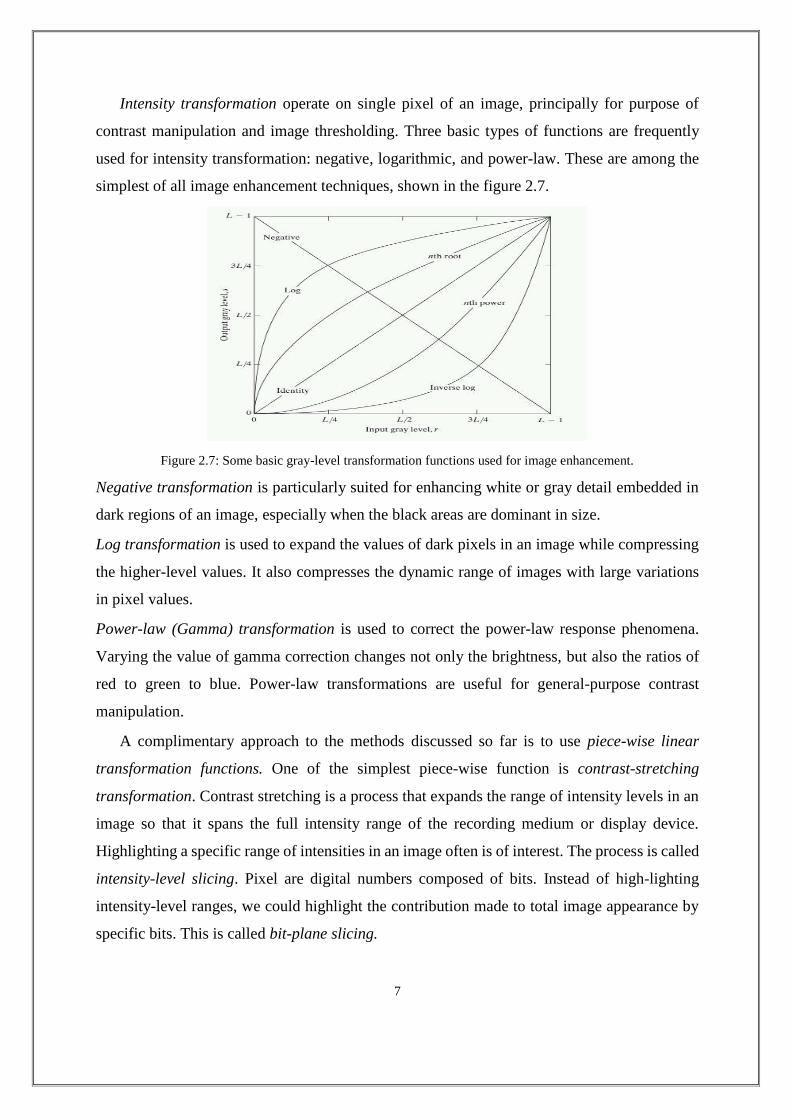
Image acquisition using sensor arrays

Figure 2.5 shows individual sensors arranged in the form of a 2-D array. Numerous

electromagnetic and some ultrasonic sensing devices frequently are arranged in an array format.

This is also the predominant arrangement found in digital cameras. The principal manner in

which array sensors are used is shown in figure 2.6. This figure shows the energy from an

illumination source being reflected from a scene element.

5

The first function performed by the imaging system shown is to collect the incoming energy

and focus it onto an image plane.

Figure 2.5: Array Sensor

If the illumination is light, the front end of the imaging system is a lens, which projects the

viewed scene onto the lens focal plane. The sensor array, which is coincident with the focal

plane, produces outputs proportional to the integral of the light received at each sensor. Digital

and analog circuitry sweep these outputs and convert them to a video signal, which is then

digitized by another section of the imaging system. The output is a digital image is shown in

the figure.

Figure 2.6: An example of the digital image acquisition process.

2.2 IMAGE ENHANCEMENT

The principal objective of enhancement is to process an image so that the result is more

suitable than the original image for a specific application. Image enhancement approaches fall

into two broad categories: spatial domain methods and frequency domain methods [8].

Image enhancement in spatial domain

The term spatial domain refers to the aggregate of pixels composing an image. Spatial domain

methods are procedures that operate directly on these pixels. Two principal categories of spatial

processing are: intensity transformation and spatial filtering.

6

Intensity transformation operate on single pixel of an image, principally for purpose of

contrast manipulation and image thresholding. Three basic types of functions are frequently

used for intensity transformation: negative, logarithmic, and power-law. These are among the

simplest of all image enhancement techniques, shown in the figure 2.7.

Figure 2.7: Some basic gray-level transformation functions used for image enhancement.

Negative transformation is particularly suited for enhancing white or gray detail embedded in

dark regions of an image, especially when the black areas are dominant in size.

Log transformation is used to expand the values of dark pixels in an image while compressing

the higher-level values. It also compresses the dynamic range of images with large variations

in pixel values.

Power-law (Gamma) transformation is used to correct the power-law response phenomena.

Varying the value of gamma correction changes not only the brightness, but also the ratios of

red to green to blue. Power-law transformations are useful for general-purpose contrast

manipulation.

A complimentary approach to the methods discussed so far is to use piece-wise linear

transformation functions. One of the simplest piece-wise function is contrast-stretching

transformation. Contrast stretching is a process that expands the range of intensity levels in an

image so that it spans the full intensity range of the recording medium or display device.

Highlighting a specific range of intensities in an image often is of interest. The process is called

intensity-level slicing. Pixel are digital numbers composed of bits. Instead of high-lighting

intensity-level ranges, we could highlight the contribution made to total image appearance by

specific bits. This is called bit-plane slicing.

7

Spatial filtering deals with performing operations such as image sharpening, by working in

the neighborhood of every pixel in an image. Filtering creates a new pixel with coordinates

equal to the coordinates of the center of the neighborhood, and whose value is the result of the

filtering operation. A processed (filtered) image is generated as the center of the filter visits

each pixel in the input image.

Smoothing filters are used for blurring and for noise reduction. Blurring is used in

preprocessing tasks, such as removal of small details from an image prior to object extraction

and bridging of small gaps in lines or curves. Noise reduction can be accomplished by bluring

with linear filter. The output of smoothing is simply the average of the pixels contained in the

neighborhood of the filter mask. These filters sometimes are called averaging filters.

The principal objective of sharpening filters is to highlight transitions in intensity. Uses of

image sharpening vary and include applications ranging from electronic printing and medical

imaging to industrial inspection and autonomous guidance in military systems.

Image enhancement in frequency domain

Filtering techniques in the frequency domain are based on modifying the Fourier transform

to achieve a specific objective and then computing the inverse DFT to get us back to the image

domain.

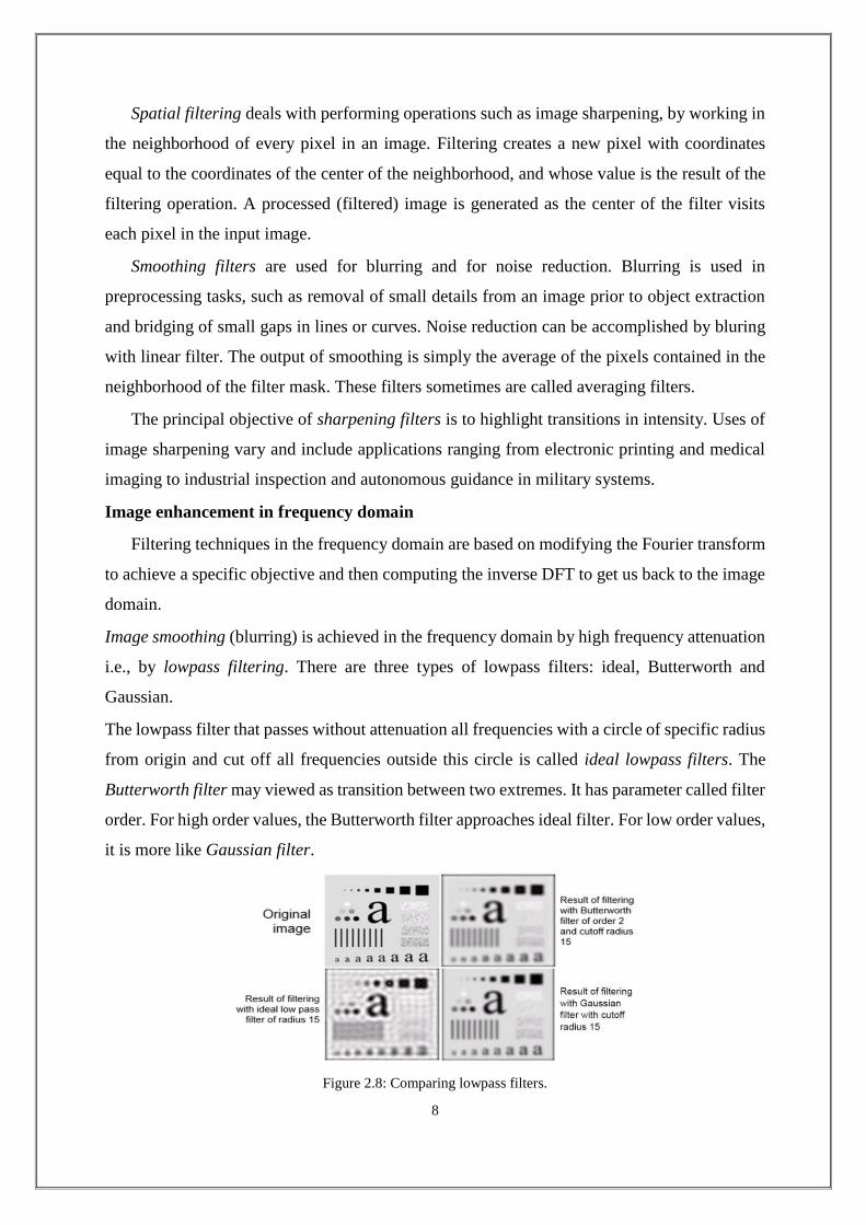
Image smoothing (blurring) is achieved in the frequency domain by high frequency attenuation

i.e., by lowpass filtering. There are three types of lowpass filters: ideal, Butterworth and

Gaussian.

The lowpass filter that passes without attenuation all frequencies with a circle of specific radius

from origin and cut off all frequencies outside this circle is called ideal lowpass filters. The

Butterworth filter may viewed as transition between two extremes. It has parameter called filter

order. For high order values, the Butterworth filter approaches ideal filter. For low order values,

it is more like Gaussian filter.

Figure 2.8: Comparing lowpass filters.

8

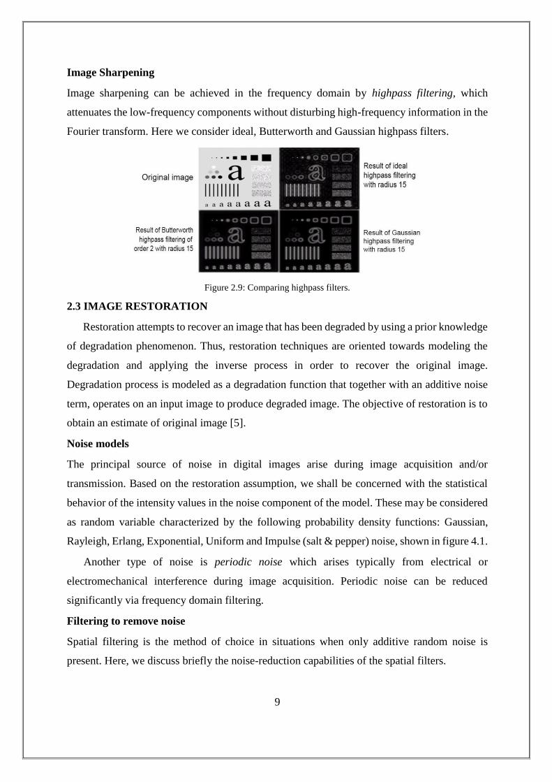
Image Sharpening

Image sharpening can be achieved in the frequency domain by highpass filtering, which

attenuates the low-frequency components without disturbing high-frequency information in the

Fourier transform. Here we consider ideal, Butterworth and Gaussian highpass filters.

Figure 2.9: Comparing highpass filters.

2.3 IMAGE RESTORATION

Restoration attempts to recover an image that has been degraded by using a prior knowledge

of degradation phenomenon. Thus, restoration techniques are oriented towards modeling the

degradation and applying the inverse process in order to recover the original image.

Degradation process is modeled as a degradation function that together with an additive noise

term, operates on an input image to produce degraded image. The objective of restoration is to

obtain an estimate of original image [5].

Noise models

The principal source of noise in digital images arise during image acquisition and/or

transmission. Based on the restoration assumption, we shall be concerned with the statistical

behavior of the intensity values in the noise component of the model. These may be considered

as random variable characterized by the following probability density functions: Gaussian,

Rayleigh, Erlang, Exponential, Uniform and Impulse (salt & pepper) noise, shown in figure 4.1.

Another type of noise is periodic noise which arises typically from electrical or

electromechanical interference during image acquisition. Periodic noise can be reduced

significantly via frequency domain filtering.

Filtering to remove noise

Spatial filtering is the method of choice in situations when only additive random noise is

present. Here, we discuss briefly the noise-reduction capabilities of the spatial filters.

9

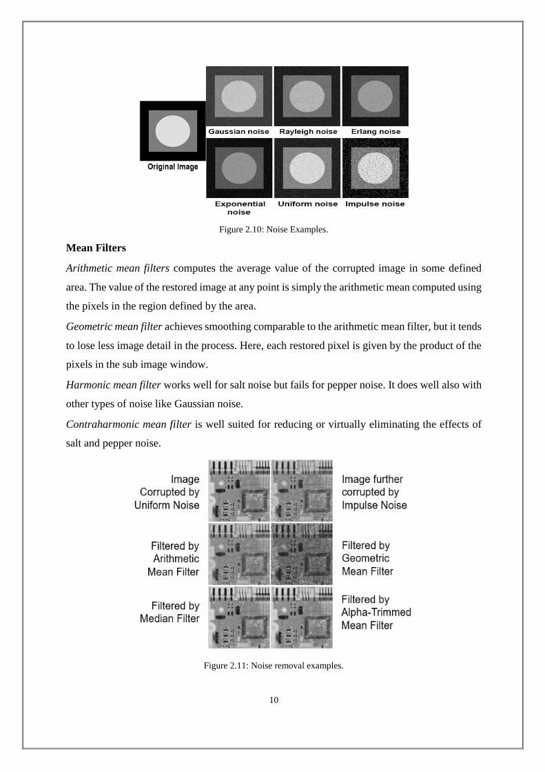
Figure 2.10: Noise Examples.

Mean Filters

Arithmetic mean filters computes the average value of the corrupted image in some defined

area. The value of the restored image at any point is simply the arithmetic mean computed using

the pixels in the region defined by the area.

Geometric mean filter achieves smoothing comparable to the arithmetic mean filter, but it tends

to lose less image detail in the process. Here, each restored pixel is given by the product of the

pixels in the sub image window.

Harmonic mean filter works well for salt noise but fails for pepper noise. It does well also with

other types of noise like Gaussian noise.

Contraharmonic mean filter is well suited for reducing or virtually eliminating the effects of

salt and pepper noise.

Figure 2.11: Noise removal examples.

10

Order-statistic Filters

These are spatial filters whose response is based on ordering (ranking) the values of pixels

contained in the image area encompassed by the filters. The ranking result determines the

response of the filter.

Median filter replaces the value of a pixel by the median of the intensity levels in the neighbo-

rhood of that pixel. For certain types of random noise, they provide excellent noise-reduction

capabilities, with considerably less blurring than linear smoothing filters of similar size.

Max and Min filters is useful for finding the brightest and darkest points in an image. It is good

for salt and pepper noise.

Midpoint filter simply computes the midpoint between the maximum and minimum values in

the area encompassed by the filter. This filter combines the order-statistic and averaging. It

works best for randomly distributed noise, like Gaussian and Uniform noise.

Alpha-trimmed mean filters is useful in situations involving multiple types of noise, such as

combination of salt and pepper noise and Gaussian noise.

Bandreject Filter

Periodic noise is analyzed and filtered using quite effectively using frequency domain filtering

techniques. Bandreject filter is used for this purpose. It is used for noise removal applications

where the general location of the noise components in the frequency domain is approximately

known.

11

CHAPTER 3

COLOR IMAGE PROCESSING

Color image processing is divided into two categories: full-color and pseudocolor image

processing. In the first category, the images in question are typically acquired with a full-color

sensor, such as a color TV camera or color scanner. In the second category, the problem is one

of assigning a color to a particular monochrome intensity or range of intensities [6].

3.1 PSEUDOCOLOR IMAGE PROCESSING

Pseudocolor image processing consists of assigning color to grey values based on a

specified criterion. The term pseudo or false color is used to differentiate the process of

assigning colors to monochrome images from the processes associated with true color images.

The principal use of pseudocolor is for human visualization and interpretation of grey-scale

events in an image or sequence of images.

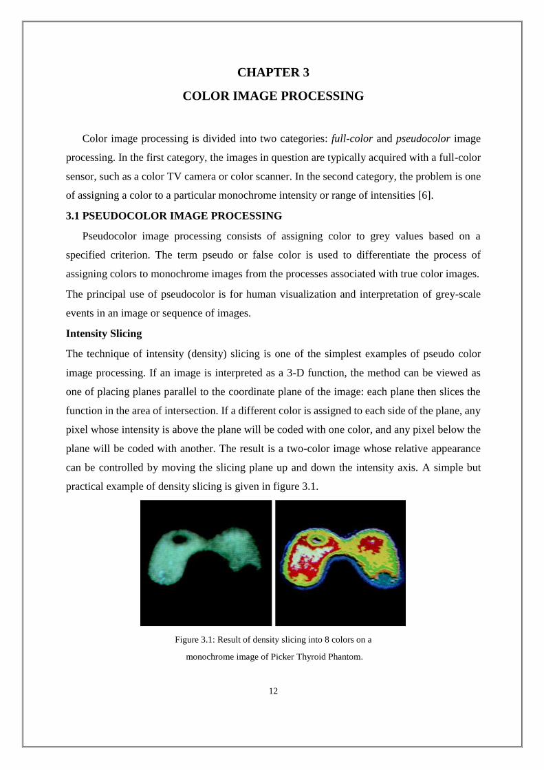
Intensity Slicing

The technique of intensity (density) slicing is one of the simplest examples of pseudo color

image processing. If an image is interpreted as a 3-D function, the method can be viewed as

one of placing planes parallel to the coordinate plane of the image: each plane then slices the

function in the area of intersection. If a different color is assigned to each side of the plane, any

pixel whose intensity is above the plane will be coded with one color, and any pixel below the

plane will be coded with another. The result is a two-color image whose relative appearance

can be controlled by moving the slicing plane up and down the intensity axis. A simple but

practical example of density slicing is given in figure 3.1.

Figure 3.1: Result of density slicing into 8 colors on a

monochrome image of Picker Thyroid Phantom.

12

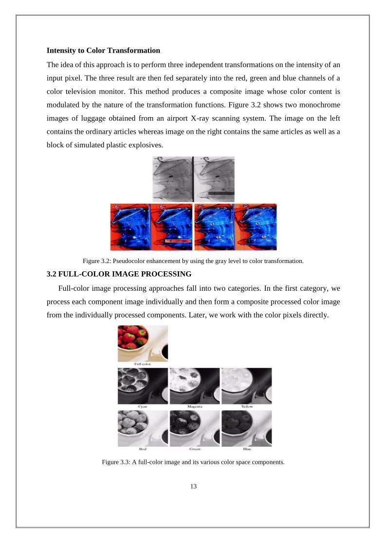
Intensity to Color Transformation

The idea of this approach is to perform three independent transformations on the intensity of an

input pixel. The three result are then fed separately into the red, green and blue channels of a

color television monitor. This method produces a composite image whose color content is

modulated by the nature of the transformation functions. Figure 3.2 shows two monochrome

images of luggage obtained from an airport X-ray scanning system. The image on the left

contains the ordinary articles whereas image on the right contains the same articles as well as a

block of simulated plastic explosives.

Figure 3.2: Pseudocolor enhancement by using the gray level to color transformation.

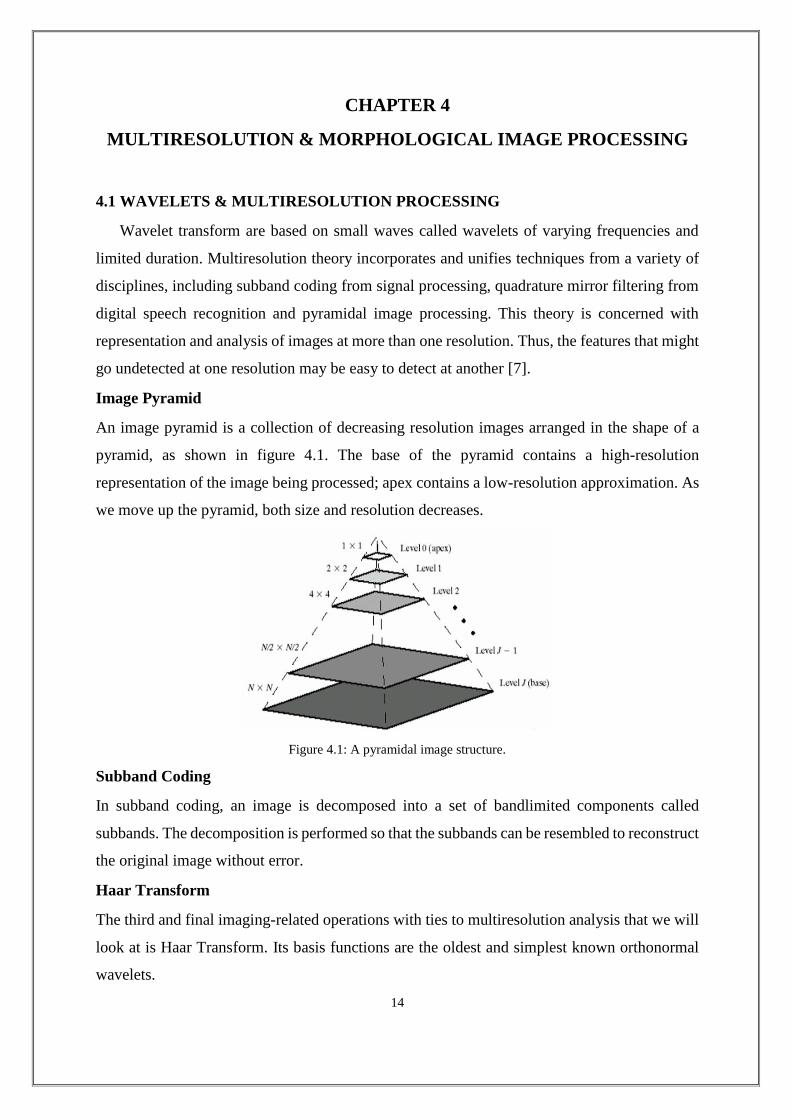
3.2 FULL-COLOR IMAGE PROCESSING

Full-color image processing approaches fall into two categories. In the first category, we

process each component image individually and then form a composite processed color image

from the individually processed components. Later, we work with the color pixels directly.

Figure 3.3: A full-color image and its various color space components.

13

CHAPTER 4

MULTIRESOLUTION & MORPHOLOGICAL IMAGE PROCESSING

4.1 WAVELETS & MULTIRESOLUTION PROCESSING

Wavelet transform are based on small waves called wavelets of varying frequencies and

limited duration. Multiresolution theory incorporates and unifies techniques from a variety of

disciplines, including subband coding from signal processing, quadrature mirror filtering from

digital speech recognition and pyramidal image processing. This theory is concerned with

representation and analysis of images at more than one resolution. Thus, the features that might

go undetected at one resolution may be easy to detect at another [7].

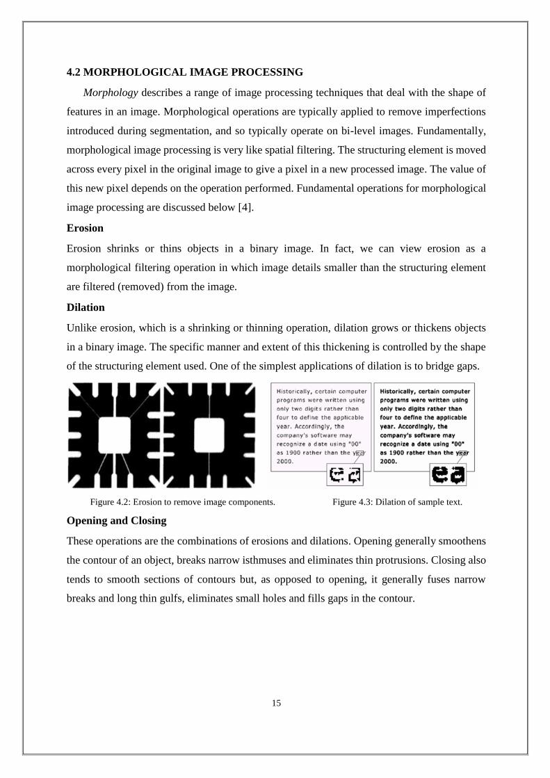
Image Pyramid

An image pyramid is a collection of decreasing resolution images arranged in the shape of a

pyramid, as shown in figure 4.1. The base of the pyramid contains a high-resolution

representation of the image being processed; apex contains a low-resolution approximation. As

we move up the pyramid, both size and resolution decreases.

Figure 4.1: A pyramidal image structure.

Subband Coding

In subband coding, an image is decomposed into a set of bandlimited components called

subbands. The decomposition is performed so that the subbands can be resembled to reconstruct

the original image without error.

Haar Transform

The third and final imaging-related operations with ties to multiresolution analysis that we will

look at is Haar Transform. Its basis functions are the oldest and simplest known orthonormal

wavelets.

14

4.2 MORPHOLOGICAL IMAGE PROCESSING

Morphology describes a range of image processing techniques that deal with the shape of

features in an image. Morphological operations are typically applied to remove imperfections

introduced during segmentation, and so typically operate on bi-level images. Fundamentally,

morphological image processing is very like spatial filtering. The structuring element is moved

across every pixel in the original image to give a pixel in a new processed image. The value of

this new pixel depends on the operation performed. Fundamental operations for morphological

image processing are discussed below [4].

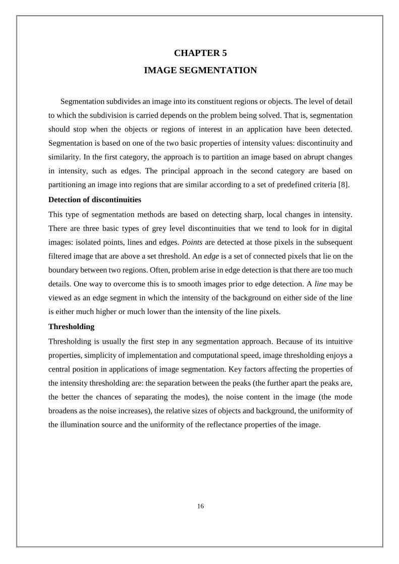
Erosion

Erosion shrinks or thins objects in a binary image. In fact, we can view erosion as a

morphological filtering operation in which image details smaller than the structuring element

are filtered (removed) from the image.

Dilation

Unlike erosion, which is a shrinking or thinning operation, dilation grows or thickens objects

in a binary image. The specific manner and extent of this thickening is controlled by the shape

of the structuring element used. One of the simplest applications of dilation is to bridge gaps.

Figure 4.2: Erosion to remove image components. Figure 4.3: Dilation of sample text.

Opening and Closing

These operations are the combinations of erosions and dilations. Opening generally smoothens

the contour of an object, breaks narrow isthmuses and eliminates thin protrusions. Closing also

tends to smooth sections of contours but, as opposed to opening, it generally fuses narrow

breaks and long thin gulfs, eliminates small holes and fills gaps in the contour.

15

CHAPTER 5

IMAGE SEGMENTATION

Segmentation subdivides an image into its constituent regions or objects. The level of detail

to which the subdivision is carried depends on the problem being solved. That is, segmentation

should stop when the objects or regions of interest in an application have been detected.

Segmentation is based on one of the two basic properties of intensity values: discontinuity and

similarity. In the first category, the approach is to partition an image based on abrupt changes

in intensity, such as edges. The principal approach in the second category are based on

partitioning an image into regions that are similar according to a set of predefined criteria [8].

Detection of discontinuities

This type of segmentation methods are based on detecting sharp, local changes in intensity.

There are three basic types of grey level discontinuities that we tend to look for in digital

images: isolated points, lines and edges. Points are detected at those pixels in the subsequent

filtered image that are above a set threshold. An edge is a set of connected pixels that lie on the

boundary between two regions. Often, problem arise in edge detection is that there are too much

details. One way to overcome this is to smooth images prior to edge detection. A line may be

viewed as an edge segment in which the intensity of the background on either side of the line

is either much higher or much lower than the intensity of the line pixels.

Thresholding

Thresholding is usually the first step in any segmentation approach. Because of its intuitive

properties, simplicity of implementation and computational speed, image thresholding enjoys a

central position in applications of image segmentation. Key factors affecting the properties of

the intensity thresholding are: the separation between the peaks (the further apart the peaks are,

the better the chances of separating the modes), the noise content in the image (the mode

broadens as the noise increases), the relative sizes of objects and background, the uniformity of

the illumination source and the uniformity of the reflectance properties of the image.

16

CHAPTER 6

IMAGE COMPRESSION & REPRESENTATION

6.1 IMAGE COMPRESSION

Image compression, the science and art of reducing the amount of data required to represent

an image, is one of the most useful and commercially successful technologies in the field of

digital image processing. The number of images that are compressed and decompressed daily

are staggering, and compressions and decompressions themselves are virtually invisible to the

user.

To better understand the need for compact image representation, consider the amount of

data required to represent a two-hour standard definition (SD) movie using 720 X 480 X 24 bit

pixel arrays. A digital movie is a sequence of video frames in which each frame is a full-color

still image. Because video players must display the frames sequentially at rates near 30fps

(frames per second), SD digital video consists of 224 GB of data. Twenty-seven 8.5 GB dual-

layer DVDs are needed to store it. To put a two-hour movie on a single DVD, each frame must

be compressed on average by a factor of 26.3. The compression must be higher for high

definition (HD) television where image resolutions reach 1920 X 1080 X 24 bits/image.

Compression can reduce transmission time by a factor of 2 to 10 or more. In the same way, the

number of uncompressed full-color images that an 8-megapixel digital camera can store on a

1-GB flash memory card can be increased. In addition to these applications, image compression

plays an important role in many other areas including tele video conferencing, remote sensing,

document and medical imaging and facsimile transmission.

Thus most frequently used compressing techniques used are discussed below. Compression is

achieved when one or more redundancy is reduced or eliminated. The computer-generated

image in figure 6.1 exhibit each of these fundamental redundancies [9].

Coding Redundancy

A code is a system of symbols (letters, numbers, bits) used to represent a body of information

or set of events. Each piece of information or event is assigned a sequence of code symbols

called a code word. The number of symbols in each code word is its length. The 8-bit codes

that are used to represent the intensities in most 2-D intensity arrays contain more bits than are

needed to represent the intensities.

17

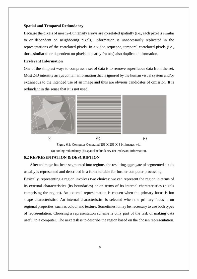
Spatial and Temporal Redundancy

Because the pixels of most 2-D intensity arrays are correlated spatially (i.e., each pixel is similar

to or dependent on neighboring pixels), information is unnecessarily replicated in the

representations of the correlated pixels. In a video sequence, temporal correlated pixels (i.e.,

those similar to or dependent on pixels in nearby frames) also duplicate information.

Irrelevant Information

One of the simplest ways to compress a set of data is to remove superfluous data from the set.

Most 2-D intensity arrays contain information that is ignored by the human visual system and/or

extraneous to the intended use of an image and thus are obvious candidates of omission. It is

redundant in the sense that it is not used.

(a) (b) (c)

Figure 6.1: Computer Generated 256 X 256 X 8 bit images with

(a) coding redundancy (b) spatial redundancy (c) irrelevant information.

6.2 REPRESENTATION & DESCRIPTION

After an image has been segmented into regions, the resulting aggregate of segmented pixels

usually is represented and described in a form suitable for further computer processing.

Basically, representing a region involves two choices: we can represent the region in terms of

its external characteristics (its boundaries) or on terms of its internal characteristics (pixels

comprising the region). An external representation is chosen when the primary focus is ion

shape characteristics. An internal characteristics is selected when the primary focus is on

regional properties, such as colour and texture. Sometimes it may be necessary to use both types

of representation. Choosing a representation scheme is only part of the task of making data

useful to a computer. The next task is to describe the region based on the chosen representation.

18

Representation

Chain codes are used to represent a boundary by a connected sequence of straight-line segments

of specified length and direction. Typically, this representation is based on 4- or 8-connectivity

of the segments. The direction of each segment is coded by a numbering scheme. A boundary

code formed as a sequence of such directional numbers is referred to as a Freeman chain code.

A signature 1-D functional representation of a boundary and may be generated in various ways.

One of the simplest is to plot the distance from the centroid to the boundary as a function of

angle. An important approach to representing the structural shape of a plane region is to reduce

it to a graph. This reduction may be accomplished by obtaining the skeleton of the region via a

thinning (skeletonizing) algorithm. Thinning procedures play central role in a broad range of

problems in image processing, ranging from automated inspection of printed circuit boards to

counting of asbestos fibres in air filters.

Boundary Descriptors

The length of a boundary is one of its simplest descriptors. The number of pixels along a

boundary gives a rough approximation of its length. The value of the diameter and the

orientation of a line segment connecting the two extreme points that comprise the diameter are

also useful descriptors of a boundary.

Curvature is defined as the rate of change of slope. In general, obtaining reliable measures of

curvature at a point in a digital boundary is difficult because these boundaries tend to locally

ragged. However, using the difference between the slopes of adjacent boundary segments as a

descriptor of curvature at the point of intersection of the segments sometimes proves useful.

Regional Descriptors

The area of a region is defined as the number of pixels in the region. The perimeter of a region

is the length of its boundary. Although area and perimeter are sometimes used as descriptors,

they apply primarily to situations in which the size of the regions of interest is invariant. A more

frequent use of these two descriptors is in measuring compactness of a region defined as

(perimeter)2/area. A slightly different descriptor of compactness is the circularity ratio, defined

as the ratio of the area of a region to the area of a circle having the same perimeter. Other simple

measures used as region descriptors include the mean and median of the intensity levels, the

minimum and maximum intensity values and the number of pixels with values above and below

the mean.

19

Topological Descriptors

Topological properties are useful for global descriptions of regions in the image plane.

Topology is the study of properties of a figure that are unaffected by any deformation, as long

as there is no tearing or joining of the figure. For example, if a topological descriptor is defined

by the number of holes in the region, this property obviously will not be affected by a stretching

or rotation transformation. Another topological property is the number of connected

components.

6.3 OBJECT RECOGNITION

The approaches to object or pattern recognition are divided into two principal areas:

decision-theoretic and structural. The first category deals with patterns described using

quantitative descriptors such as length, area or texture. The second category deals with

patterns best described by qualitative descriptors such as the relational descriptors.

Recognition techniques based on matching represent each class by a prototype pattern

vector. An unknown pattern is assigned to the class to which it is closest in terms of a

predefined metric. The simplest approach is the minimum distance classifier, which, as its

name implies, computes the distance between the unknown and each of the prototype vectors.

It chooses the smallest distance to make a decision. The structural methods seek to achieve

pattern recognition by capitalizing precisely on structural relationships.

20

CHAPTER 7

FIELDS OF APPLICATION

The areas of application of digital image processing are so varied that some form of

organization is desirable in attempting to capture the breadth of this field. One of the simplest

way to develop a basic understanding of the extent of image processing applications is to

categorize images according to their source (e.g., visual, X-ray and so on). The principal energy

source for images in use today is the electromagnetic energy spectrum. Images based on

radiation from the EM spectrum are the most familiar. Other important sources of energy

include acoustic, ultrasonic and electronic (in the form of electron beams used in electron

microscopy). Synthetic images, used for modelling and visualization, are generated by

computer [1].

Imaging in EM Spectrum

Major uses of imaging based on gamma rays include nuclear medicine and astronomical

observations. In nuclear medicine, the approach is to inject a patient with a radioactive isotope

that emits gamma rays as it decays. Images are produced from the emissions collected by

gamma ray detectors. Images of this sort are used to locate sites of bone pathology, such as

infections or tumours.

X-rays are among the oldest sources of EM radiation used for imaging. The best known use

of X-rays is medical diagnostics, but they also are used extensively in industry and other areas,

like astronomy. X-rays for medical and industrial imaging are generated using an X-ray tube,

which is a vacuum tube with a cathode and anode. The cathode is heated, causing free electrons

to be released. These electrons flow at high speed to the positively charged anode. When the

electrons strike a nucleus, energy is released in the form of X-ray radiation. The energy

(penetrating power) of the X-rays is controlled by a voltage applied across the anode and the

number of X-rays is controlled by a current applied to the filament in the cathode.

Applications of ultraviolet light are varied. They include lithography, industrial inspection,

microscopy, lasers, biological imaging and astronomical observations. Ultraviolet light is used

in fluorescence microscopy, one of the fastest growing areas of microscopy. The basic task of

the fluorescence microscope is to use an excitation light to irradiate a prepared specimen and

then to separate the much weaker radiating fluorescent light from the brighter excitation light.

21

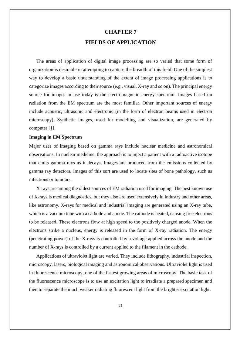
Thus, only the emission light reaches the eye or other detector. The resulting fluorescing areas

shine against a dark background with sufficient contrast to permit detection. The darker the

background of the non-fluorescing material, the more efficient the instrument.

Figure 7.1: Images of the Crab Pulsar (in the centre of images) covering the EM spectrum.

Other Imaging Modalities

Although imaging in the electromagnetic spectrum is dominant by far, there are a number of

other imaging modalities that also are important. Imaging using “sound” finds application in

geological exploration, industry, and medicine. Geological applications use sound in the low

end of the sound spectrum (hundreds of Hertz) while imaging in other areas use ultrasound

(millions of Hertz).The most important commercial applications of image processing in

geology are in mineral and oil exploration.

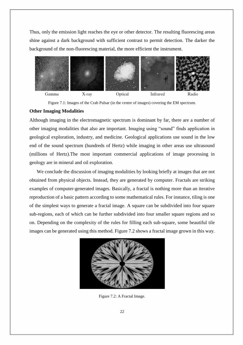
We conclude the discussion of imaging modalities by looking briefly at images that are not

obtained from physical objects. Instead, they are generated by computer. Fractals are striking

examples of computer-generated images. Basically, a fractal is nothing more than an iterative

reproduction of a basic pattern according to some mathematical rules. For instance, tiling is one

of the simplest ways to generate a fractal image. A square can be subdivided into four square

sub-regions, each of which can be further subdivided into four smaller square regions and so

on. Depending on the complexity of the rules for filling each sub-square, some beautiful tile

images can be generated using this method. Figure 7.2 shows a fractal image grown in this way.

Figure 7.2: A Fractal Image.

22

CONCLUSION

Having concluded study of the material in the preceding eleven chapters, we are now in a

position of being able to understand the principal areas panning the field of digital image

processing, both from a theoretical point of view as well as practical point of view. The main

purpose of the material was to provide a sense of perspective about the origins of digital image

processing and more important about the current and future areas of application of this

technology. Care was taken throughout all discussion to lay a solid foundation upon which

further study of this and related fields could be based. Although the coverage of the topics was

necessarily incomplete due to space limitations, it should have left you with a clear impression

of the breadth and practical scope of digital image processing. Given the task-specific nature of

many imaging problems, a clear understanding of basic principles enhances significantly the

chances for their successful solution.

23

REFERENCES

[1] Andrews, H. C. [1970]. Computer Techniques in Image Processing, Academic Press, New

York.

[2] Baxes, G.A [1994]. Digital Image Processing: Principals and Applications, John Wiley &

Sons, New York.

[3] Gonzalez, R. C. and Woods, R. E. [2002]. Digital Image Processing, 2nd ed., Prentice Hall,

Upper Saddle River, NJ.

[4] Jain, A.K [1989]. Fundamentals of Digital Image Processing, Prentice Hall, Upper Saddle

River, NJ.

[5] Petrou, M. and Bosdogianni, P.[1999]. Image Processing: The Fundamentals. John Wiley

& Sons, New York.

[6] Pratt, W.K. [1991] Digital Image Processing, 2nd ed., Wiley-Interscience, New York.

[7] Russ, J.C.[1999]. The Image Processing Handbook, 3rd ed., CRC Press, Boca Raton, FL.

[8] Schalkoff, R. J. [1989]. Digital Image Processing and Computer Vision, John Wiley &

Sons, New York.

[9] Umabaugh, S. E. [2005]. Computer Imaging: Digital Image Analysis and Processing, CRC

Press, Boca Raton, FL.

24