Development of Simplified Models of Doubly-Fed Induction Generators (DFIG) A contribution towards standardized models for voltage and tran- sient stability analysis Master of Science Thesis MICHAEL A. S NYDER Department of Energy and Environment Division of Electric Power Engineering CHALMERS UNIVERSITY OF TECHNOLOGY G¨ oteborg, Sweden 2012 Report No. xxxx.xx

Welcome message from author
This document is posted to help you gain knowledge. Please leave a comment to let me know what you think about it! Share it to your friends and learn new things together.
Transcript

Development of Simplified Modelsof Doubly-Fed Induction Generators(DFIG)A contribution towards standardized models for voltage andtran-sient stability analysisMaster of Science Thesis
M ICHAEL A. SNYDER
Department of Energy and EnvironmentDivision of Electric Power EngineeringCHALMERS UNIVERSITY OF TECHNOLOGY
Goteborg, Sweden 2012Report No. xxxx.xx

REPORT NO. xxxx.xx
Development of Simplified Models ofDoubly-Fed Induction Generators
(DFIG)A contribution towards standardized models for voltage and
transient stability analysis
MICHAEL A. SNYDER
Department of Energy and EnvironmentDivision of Electric Power Engineering
CHALMERS UNIVERSITY OF TECHNOLOGYGoteborg, Sweden 2012

Development of Simplified Models of Doubly-Fed Induction Generators (DFIG)A contribution towards standardized models for voltage andtransient stability analysisMICHAEL A. SNYDER
c© MICHAEL A. SNYDER, 2012.
Technical Report no. xxxx.xxDepartment of Energy and EnvironmentDivision of Electric Power EngineeringChalmers University of TechnologySE–412 96 GoteborgSwedenTelephone +46 (0)31–772 1000
Cover:Text concerning the cover illustration. In this case: Three-phase voltage.
Chalmers Bibliotek, ReproserviceGoteborg, Sweden 2012

Development of Simplified Models of Doubly-Fed Induction Generators (DFIG)A contribution towards standardized models for voltage andtransient stability analysisMICHAEL A. SNYDERDepartment of Energy and EnvironmentDivision of Electric Power EngineeringChalmers University of Technology
Abstract
With the increasing amounts of wind power being installed onelectrical grids, the characterization ofwind turbines during all operating conditions is essentialfor system operators to ensure security and stabilityfor their customers. This characterization must be achieved by appropriate models of various wind turbinetechnologies that can accurately depict the interaction between wind turbines and the interconnected powersystem. Of critical importance and the focus of this thesis is the response of wind turbines during a grid fault,and specifically the wind turbines’ effect on voltage and transient stability through the control of reactivepower (Q) support. The DFIG wind turbine is the focus of this thesis, as it presents a more complicatedmodel and response to transient events and thus warrants further research in the pursuit of a standardizedsimplified model for the purposes of voltage and transient stability analysis.
The proposed model is developed specifically for dynamic simulations in PSS/E power system sim-ulation tool, which is a positive-sequence phasor time-domain analysis. The simulation tool is limited toa 10ms time step. Therefore there is a need to simplify the model to a level that can be depicted at thisgranularity but also maintain a fast simulation time for implementation in large network analyses.
A 5th order model of the DFIG wind turbine is introduced through the fundamental electrical equationsthat describe the machine. The control of the machine is described, including the use of an active power (P)controller, reactive power (Q) controller, a rotor speed controller, and a torque controller. A rotor voltagelimitation is imposed and the effects are studied.
The stability of the DFIG with current controller is analyzed. The DFIG is recognized as a poorlydamped machine with poles naturally occurring near the linefrequency (50 Hz). These poorly dampedpoles are further evaluated through sensitivity analyses of model parameters and controller settings. A fluxdamping term is discussed and implemented in the DFIG detailed model. The results show successfuldamping for small disturbances but a high sensitivity to grid voltage dips.
The DC-chopper protection of the DFIG rotor circuit is analyzed. A simplified model for the DC-chopper protection is proposed that neglects the DC-link voltage controller and the control of the grid-sideconverter but instead focuses on the effects of the rotor-side converter losing controllability and entering intodiode rectifier operation. Any imbalance of rotor circuit power and grid-side converter power is assumed tobe effectively burned in the DC crowbar via a properly controlled DC-chopper and DC-link voltage.
The 5th order model is compared to a more detailed model developed in PSCAD. In previous research[1], the PSCAD model has been validated against field measurements for a DFIG wind turbine experiencingboth a shallow and deep voltage dip. The 5th order model of this thesis shows reasonable accuracy to thePSCAD model but is not able to fully synchronize with the model. Step responses of the DFIG machinemodel in PSCAD was studied and compared to the 5th order DFIG machine designed in Matlab/Simulinkto further analyze possible reasons for the differences in the two models.
iii

The 5th order model is simplified into a set of algebraic equations with a Q controller, based on severalassumptions. The goal of the simplified model is for implementation in PSS/E dynamic simulations withfast simulation times in complex power networks. The simplified model is compared to the detailed modeland shows reasonable accuracy in depicting the general response to voltage dips for the three operatingconditions (sub-synchronous, synchronous, and super-synchronous).
The machine is modeled with a fixed rotor speed and compared tothe 5th order model with a variablerotor speed.
Keywords: wind turbine, simplified model, Doubly Fed Induction Generator, DFIG, power system sta-bility, voltage stability, PSSE
Index Terms: wind turbine, simplified model, Doubly Fed Induction Generator, DFIG, power systemstability, voltage stability, PSSE
iv

Acknowledgements
This work has been carried out at the Department of Energy andEnvironment at Chalmers University ofTechnology. A sincere and special thanks to Peiyuan Chen, ashis dedication and passion to teach created anenvironment for success and an enjoyable learning atmosphere. A special thanks to Massimo Bongiorno forhis guidance and focus on understanding the fundamental concepts of this thesis, and for his dedication torepetitive teaching with patience. Thank you to Stefan Lundberg for his never-ending patience and opennessto unscheduled walk-ins, for his explanations around control theory, DFIG theory, and Matlab/Simulinkmodel development, and of course for the unplanned and informal adoption of me as his masters thesisstudent.
A heart felt thank you to my wife, Mandy, for her patience and her never ending support throughout mytime at Chalmers. A special smile and thank you to my son, Elliot, who gives me inspiration and excitementevery day. Although you cannot read this yet, someday you will, and hopefully you will think it is prettycool.
Michael A. SnyderGoteborg, Sweden, 2012
v

vi

Contents
Abstract iii
Acknowledgements v
Contents vii
1 Introduction 1
1.1 Background and Motivation . . . . . . . . . . . . . . . . . . . . . . . . .. . . . . . . . 1
1.2 Description of Wind Turbine Generator Types . . . . . . . . . .. . . . . . . . . . . . . . 2
1.2.1 Fixed Speed Wind Turbine . . . . . . . . . . . . . . . . . . . . . . . . .. . . . . 3
1.2.2 Variable Speed Wind Turbine with Variable Rotor Resistance . . . . . . . . . . . . 4
1.2.3 Variable Speed Wind Turbine with Doubly Fed InductionGenerator . . . . . . . . 5
1.2.4 Variable Speed Wind Turbine with Full Power Converter(FPC) . . . . . . . . . . 6
1.3 Problem Formulation . . . . . . . . . . . . . . . . . . . . . . . . . . . . . .. . . . . . . 6
1.3.1 Objectives and Tasks . . . . . . . . . . . . . . . . . . . . . . . . . . . .. . . . . 7
1.3.2 Methods . . . . . . . . . . . . . . . . . . . . . . . . . . . . . . . . . . . . . . . 8
2 Grid Codes for Grid Integration of Wind Farms 9
2.1 Dynamic requirements for grid integration of wind farms. . . . . . . . . . . . . . . . . . 9
2.2 E.ON Grid Code Requirements . . . . . . . . . . . . . . . . . . . . . . . .. . . . . . . . 10
3 DFIG Detailed Model 13
3.1 The Doubly Fed Induction Generator (DFIG) . . . . . . . . . . . .. . . . . . . . . . . . 14
3.1.1 Torque production in the DFIG . . . . . . . . . . . . . . . . . . . . .. . . . . . . 15
3.1.2 Rotor side converter (RSC) . . . . . . . . . . . . . . . . . . . . . . .. . . . . . . 15
3.1.3 Grid side converter (GSC) . . . . . . . . . . . . . . . . . . . . . . . .. . . . . . 16
3.1.4 Power flow in the DFIG . . . . . . . . . . . . . . . . . . . . . . . . . . . . .. . 16
3.1.5 DC-link chopper / DC crowbar . . . . . . . . . . . . . . . . . . . . . .. . . . . . 18
vii

Contents
3.1.6 AC Crowbar . . . . . . . . . . . . . . . . . . . . . . . . . . . . . . . . . . . . .18
3.2 5th Order Machine Model . . . . . . . . . . . . . . . . . . . . . . . . . . . .. . . . . . 19
3.2.1 Transient Model . . . . . . . . . . . . . . . . . . . . . . . . . . . . . . . .. . . 20
3.2.2 Γ-equivalent Model . . . . . . . . . . . . . . . . . . . . . . . . . . . . . . . . . . 23
3.3 Control of DFIG Machine . . . . . . . . . . . . . . . . . . . . . . . . . . . .. . . . . . 25
3.3.1 Rotor Current Controller . . . . . . . . . . . . . . . . . . . . . . . .. . . . . . . 25
3.3.2 Active DampingRa . . . . . . . . . . . . . . . . . . . . . . . . . . . . . . . . . 27
3.3.3 Rotor Current Reference Calculation . . . . . . . . . . . . . .. . . . . . . . . . . 28
3.3.4 Reactive Power (Q) Controller . . . . . . . . . . . . . . . . . . . .. . . . . . . . 29
3.3.5 Speed Controller . . . . . . . . . . . . . . . . . . . . . . . . . . . . . . .. . . . 30
3.3.6 Active Power (P) Controller . . . . . . . . . . . . . . . . . . . . . .. . . . . . . 32
4 Converter limitations and model implementation of DC-chopper 33
4.1 Rotor voltage limitation . . . . . . . . . . . . . . . . . . . . . . . . . .. . . . . . . . . . 33
4.2 Rotor current limitation . . . . . . . . . . . . . . . . . . . . . . . . . .. . . . . . . . . . 34
4.3 Grid-side converter current limitation . . . . . . . . . . . . .. . . . . . . . . . . . . . . 39
4.4 Model implementation of DC-chopper . . . . . . . . . . . . . . . . .. . . . . . . . . . . 40
4.4.1 Regaining control of the RSC . . . . . . . . . . . . . . . . . . . . . .. . . . . . 42
5 Evaluation of 5th Order Model against PSCAD Detailed Model 47
5.1 Damping analysis of the DFIG model . . . . . . . . . . . . . . . . . . .. . . . . . . . . 50
6 DFIG Simplified Model 57
6.1 Review of simplified DFIG models for stability studies . .. . . . . . . . . . . . . . . . . 57
6.2 List of Model Simplifications . . . . . . . . . . . . . . . . . . . . . . .. . . . . . . . . . 58
6.3 Comparison of 5th order machine model to 3rd order machine model . . . . . . . . . . . . 59
6.4 Comparison of 3rd order machine model to 2nd order machine model . . . . . . . . . . . 62
6.5 Development of the final simplified DFIG model . . . . . . . . . .. . . . . . . . . . . . 62
6.6 Comparison of 2nd order machine model to machine modeledas a set of algebraic equations 66
7 Conclusions and Future Work 71
7.1 Conclusions . . . . . . . . . . . . . . . . . . . . . . . . . . . . . . . . . . . . .. . . . . 71
7.2 Future work . . . . . . . . . . . . . . . . . . . . . . . . . . . . . . . . . . . . . .. . . . 73
References 75
viii

Contents
A Results from comparison of model simplifications 77
A.1 Comparison of 5th order model to 3rd order model . . . . . . . .. . . . . . . . . . . . . 78
A.2 Comparison of 3rd order model to 2nd order model . . . . . . . .. . . . . . . . . . . . . 84
A.3 Comparison of 2nd order model to simplified model . . . . . . .. . . . . . . . . . . . . . 90
ix

Contents
x
Chapter 1
Introduction
1.1 Background and Motivation
Wind power generation has continued to increase worldwide,with the latest annual reportstating installed wind power worldwide of 239 GW at 2011 year’s end, which is enoughto cover 3% of the world’s electricity demand. Worldwide growth continues at approxi-mately 24% per year [2]. With this increase in wind power generation, their penetrationlevels and influence on utility grids has grown as well. The penetration has become sub-stantially high in particular countries, including Denmark (22%), Spain (15.4%), Portugal(21%), Ireland (10.1%), and Germany (6%). Additionally there were four German statesthat met over 40% of their energy demands via wind power [3]. These figures representannual energy production as a function of total electricitydemand, so actualpeakpene-tration could be substantially higher than these figures.
As the penetration of wind power increases, so too does the importance of ensuringthat the wind power generation does not adversely affect thepower quality, security, andreliability of each power system network, during both steady-state operation and undera contingency scenario. Therefore, traditional forms of modeling wind turbines as eitherdistributed small generators or as negative loads are no longer adequate. These traditionalrepresentations must be updated to properly model wind turbines interaction with the gridin order to properly predict security or reliability issues.
Coupled with this realization of increasing grid penetration is the action of many gridoperators to introduce more demanding grid codes for wind power interconnections. Therequirements for the dynamic performance of grid connectedwind turbines are mainlycentered around the wind turbine’s ability to stay on-line during a voltage dip, a termreferred to as fault ride-through or FRT. FRT requirements can be coupled with require-ments for reactive power support to assist with voltage stability. Wind turbine manufac-turers must incorporate this fault ride-through and reactive power support functionality
1
Chapter 1. Introduction
into their products.
This thesis will analyze the behavior of Doubly-Fed Induction Generators (DFIG) usedwith wind turbines to capture wind energy and transfer it to the grid. The DFIG has twoconnections to the grid - a direct connection to the main terminals of the stator windings,and a connection to the wound rotor windings via back-to-back voltage source converters(VSCs). The DFIGs response in the presence of grid dynamics,for example a short circuitcausing a voltage drop or varying loads and generation causing voltage and frequencydeviations, is of primary interest in this research. The DFIG has a unique response due tothese two grid connections - the rotor can be controlled quickly with the VSC, while thestator is directly coupled to the grid and therefore directly affected by voltage fluctuationsof the grid. This unique arrangement, coupled with the popularity of the DFIGs use inwind technology, makes the DFIG a critical machine to properly understand and modelin the context of grid stability analysis, as well as utilityfeasibility and planning studies.Utilities must be able to properly model both new and existing wind turbines in order topredict grid stability and security, a key to ensuring the continued growth and penetrationlevels of wind energy.
Previous research in the development of a simplified model has made certain assump-tions and simplifications. With each simplification, the model is limited and its accuracydecreased. The acceptability of this compromise is a function of the expected use and ap-plication of the model. Therefore it is essential in this research to understand the purposeof previous simplifications, state the validity of these simplifications, and determine whatsimplifications are required or not required in order to properly model the DFIG for thepurposes of grid stability analysis.
1.2 Description of Wind Turbine Generator Types
A fundamental concept in understanding wind technology is wind energy capture. Windholds in it a discrete amount of power at any given point in time, dependent in large parton the wind speed. As wind speed can vary greatly, wind turbines must be capable ofoperating over a wide wind speed range. The wind turbine can operate in one of twoways. The first is to have a relatively fixed rotational speed,in which an increase in windspeed can slightly increase the rotor speed above the synchronous speed and thus varyingthe slip. This is based purely on the torque-speed relationship of an induction machine.The wind turbine can also operate as a variable-speed machine, varying the rotor speedbased on the wind velocity. A speed controller is used to varythe pitch of the wind turbineblades during high wind speeds to reduce the power intake andprotect the wind turbine, inwhich case the rotor speed is also controlled in order to optimize the ratio of wind speedto rotor speed. The goal in varying the pitch is to maximize efficiency by optimizing a
2

1.2. Description of Wind Turbine Generator Types
term called thetip-speed ratio. The tip-speed ratio (λ) is defined as:
λ =vtip
vwind
(1.1)
wherevtip is the velocity of the blade tip andvwind is the wind velocity. The tip speedvelocity can be calculated from:
vtip = Ω× r (1.2)
whereΩ is the mechanical speed of the wind turbine andr is the radius of the circleof rotation, in this case the length of the wind turbine blade. From here it can be seen thatthe ability to maximize the aerodynamic efficiency of energycapture, is directly related tothe ability to vary the rotational speed. There are several configurations for variable speedwind turbines that allow for the generator’s rotor to operate at a variable rotational speed.
The various configurations for fixed and variable speed wind turbine generators can bebroken down into four main types to be described in the following sections.
1. Fixed Speed Wind Turbine (FSWT) with induction generator
2. Variable Speed Wind Turbine (VSWT) with variable rotor resistance
3. VSWT with Doubly-Fed Induction Generator (DFIG)
4. VSWT with Full-Power Converter (FPC)
There are common components with each of the configurations as seen in the figuresfor each. A gear box is used in between the wind turbine and generator to convert the lowerrotational speed of the turbine to a higher rotational speedfor the generator rotor. Also, astep-up transformer is used to connect the wind turbine generator to the grid, transformingthe voltage up as needed to connect to the distribution or transmission system [4] [5].
1.2.1 Fixed Speed Wind Turbine
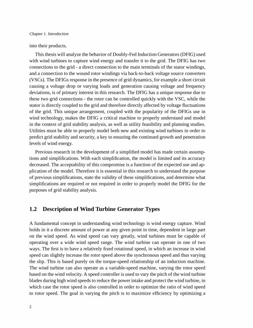
Figure 1.1 shows the basic configuration for the fixed-speed wind turbine connected tothe grid via an induction generator. The stator terminals are connected directly to thegrid, and thus the generator rotor rotates at a fixed speed based on the grid frequency andnumber of pole pairs of the machine. The turbine rotor will therefore also rotate at a fixedspeed, dependent on the rotor speed and also the turns ratio of the gear box. The inductionmachine by its nature acts to absorb reactive power (as implied by the name ”induction”),therefore capacitor banks are used to provide this reactivepower locally and minimize thereactive power drawn from the grid. Since the rotor speed is for the most part fixed, windpower variations will result in a power delivery that fluctuates and adversely affects thepower quality of the grid [5].
3
Chapter 1. Introduction
Gear-
Box
Soft
Starter
Capacitor Bank
IG
Interconnection
Transformer
Grid
Figure 1.1: Fixed Speed Wind Turbine
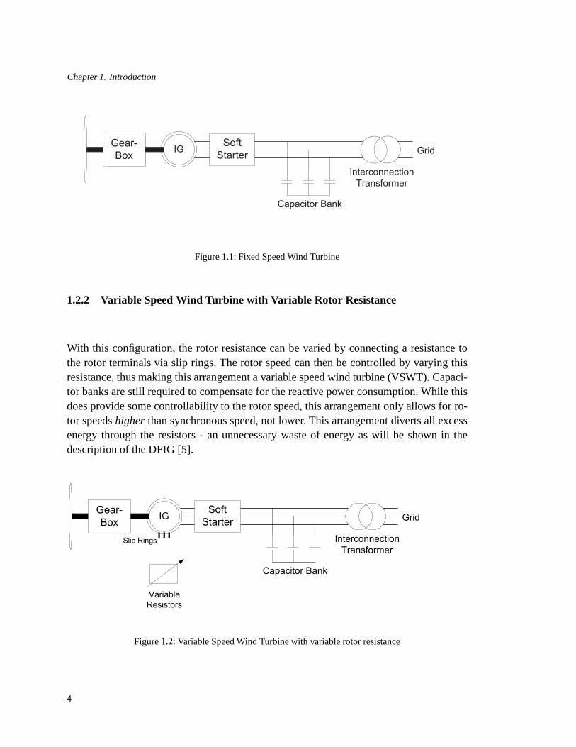
1.2.2 Variable Speed Wind Turbine with Variable Rotor Resistance
With this configuration, the rotor resistance can be varied by connecting a resistance tothe rotor terminals via slip rings. The rotor speed can then be controlled by varying thisresistance, thus making this arrangement a variable speed wind turbine (VSWT). Capaci-tor banks are still required to compensate for the reactive power consumption. While thisdoes provide some controllability to the rotor speed, this arrangement only allows for ro-tor speedshigher than synchronous speed, not lower. This arrangement diverts all excessenergy through the resistors - an unnecessary waste of energy as will be shown in thedescription of the DFIG [5].
Gear-
Box
Soft
Starter
Capacitor Bank
IG
Interconnection
Transformer
Grid
Variable
Resistors
Slip Rings
Figure 1.2: Variable Speed Wind Turbine with variable rotorresistance
4
1.2. Description of Wind Turbine Generator Types
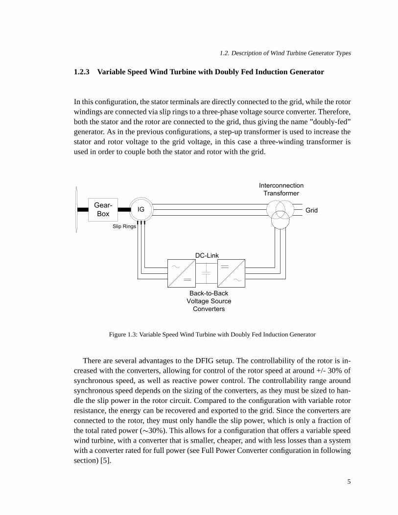
1.2.3 Variable Speed Wind Turbine with Doubly Fed InductionGenerator
In this configuration, the stator terminals are directly connected to the grid, while the rotorwindings are connected via slip rings to a three-phase voltage source converter. Therefore,both the stator and the rotor are connected to the grid, thus giving the name ”doubly-fed”generator. As in the previous configurations, a step-up transformer is used to increase thestator and rotor voltage to the grid voltage, in this case a three-winding transformer isused in order to couple both the stator and rotor with the grid.
Gear-
Box
DC-Link
IG
Interconnection
Transformer
Grid
Back-to-Back
Voltage Source
Converters
Slip Rings
Figure 1.3: Variable Speed Wind Turbine with Doubly Fed Induction Generator
There are several advantages to the DFIG setup. The controllability of the rotor is in-creased with the converters, allowing for control of the rotor speed at around +/- 30% ofsynchronous speed, as well as reactive power control. The controllability range aroundsynchronous speed depends on the sizing of the converters, as they must be sized to han-dle the slip power in the rotor circuit. Compared to the configuration with variable rotorresistance, the energy can be recovered and exported to the grid. Since the converters areconnected to the rotor, they must only handle the slip power,which is only a fraction ofthe total rated power (∼30%). This allows for a configuration that offers a variable speedwind turbine, with a converter that is smaller, cheaper, andwith less losses than a systemwith a converter rated for full power (see Full Power Converter configuration in followingsection) [5].
5

Chapter 1. Introduction
Gear-
Box
DC-Link
IG
Interconnection
Transformer
Grid
Back-to-Back
Voltage Source
Converters
Figure 1.4: Variable Speed Wind Turbine with Full Power Converter
1.2.4 Variable Speed Wind Turbine with Full Power Converter(FPC)
Figure 1.4 represents a VSWT with a full power converter. With this configuration, back-to-back VSCs are connected directly to the stator terminalsof the generator, which canbe either an induction generator or a synchronous generator. All of the power must flowfrom the generator through the converters to the grid, requiring the converters to be ratedfor the full power capacity of the generator. The power rating is one of the limiting factorsof this arrangement as it requires larger converters and components. As shown in Figure1.4, the FPC WT is connected to the grid through a step-up transformer. An AC filter isalso commonly included prior to the point of common coupling, not shown in the figurehere.
With the FPC, the machine-side converter can be used to give full controllability ofthe rotor speed, making this system very flexible. In addition, the Voltage-Source Con-verter used in this application is commonly used in other power system applications (suchas HVDC converters and STATCOMs), which makes the control and operation a well-developed and robust methodology [5].
1.3 Problem Formulation
The overall aim of this research is todevelop and verifya simplified model of the DFIGfor implementation in PSS/E that is able to properly represent the DFIG’s response in thecontext of transient stability and short term voltage stability. The simplified model willbe used in this research to study the ability of the DFIG to provide grid support throughcontrol of active power and reactive power.
6

1.3. Problem Formulation
1.3.1 Objectives and Tasks
In order to meet the aim of this research, the following objectives and associated taskswere set forth.
1. Develop adetailedmodel of the DFIG:
• Define the meaning ofdetailedin the context of this research.
• Present the equations that describe the machine.
• Design different control algorithms.
• Build the state-space model in MATLAB.
• State any assumptions or simplifications. This detailed model will still representthe VSC as a controllable DC voltage source, and will not include converterswitching dynamics.
• Study the effect of the DC-chopper and implement a model in Matlab.
2. Identify current research and efforts in the developmentof simplified DFIG modelsfor grid stability analysis:
• State the simplifications made on previous research efforts.
• State why these simplifications were made, and the impact on the simulationresults.
• State the limitations of these simplifications (what problems cannot be solvedproperly with these assumptions).
3. Study the accuracy of the model:
• Compare to a more detailed model of the DFIG which includes converter switch-ing. For this point, a pre-built PSCAD model of the DFIG system will be utilizedthat has been validated against a field measured DFIG response to voltage dips.
• Qualitative analysis to determine smallest time-step/frequency at which bothmodels are in agreement. For example, determine if the PSCADmodel simu-lation shows a significant divergence from the MATLAB model for differenttime-steps in the simulation, and determine if this is acceptable for the purposesof the system level analysis that will be required of this model.
4. Derive a simplified model from the detailed model created in MATLAB:
• Identify the purpose of the simplified model (implement in PSS/E for grid sta-bility analysis through the delivery of P and Q).
• State what simplifications can be made in order to keep this goal/objective validin the model.
7

Chapter 1. Introduction
• State how previous simplifications are/were not sufficient.
• Develop simplified models using one simplification at a time,clearly statingeach model simplification with purpose.
• Develop final simplified model as a set of algebraic equationsto describe themachine, with an active and reactive power controller.
5. Compare simplified models to the detailed model:
• Compare each simplified model to the previous model iteration, starting withthe detailed model (created in MATLAB in task 1).
• Run simulations to various voltage dips and operating points to study modelaccuracy.
• Develop conclusions regarding the impact of various model simplifications tothe accuracy and response of the model to various voltage dips and under vari-ous operating points.
• Develop conclusions on the accuracy of the final simplified model with respectto the 5th order detailed machine model. State the conditions of use the modelis valid for power system analyses, and the conditions underwhich it may notbe valid.
1.3.2 Methods
The following methods were used in the research to accomplish the previously describedobjectives and tasks.
• Power system theories and mathematical methods for the derivation of the machinemodel equations.
• State-space implementation and Matlab for modeling of differential equations.
• Internal Model Control (IMC) for design of controller.
• Verification of model against PSCAD model that is validated with field measure-ments.
8
Chapter 2
Grid Codes for Grid Integration ofWind Farms
2.1 Dynamic requirements for grid integration of wind farms
Wind power generation growth has reached a level where theirimpact to the overall powersystem cannot be neglected. Many system operators have established requirements for theinterconnection of wind farms to protect grid stability andreliability. These requirementscan be summarized into the following categories [6]:
• Operating Voltage and Frequency Range. Utilities typically require wind farms tostay connected within specific voltage and frequency windows, with specific timesassociated with different voltage and frequency deviations from nominal. For exam-ple, the wind farm will be expected to operate continuously for a certain windowaround nominal voltage and frequency, but the requirement to stay connected de-creases the further the voltage and frequency deviate from nominal. This requirementis typically represented in a table or chart format.
• Ramp Rate Control. This requirement is related to the speed at which the windfarm’s active power increases or decreases. Utilities require that a wind farm notramp up or ramp down too quickly to minimize the impact of fastactive powerfluctuations to the stability of the power system. This requirement is stated in termsof MW per minute or MW per second.
• Voltage and Reactive Power Support. Reactive power requirements vary in imple-mentation across the various grid codes. Some can be in the form of power factorcontrol, while others require reactive power transfer as a function of the voltage atthe point of interconnection.
9

Chapter 2. Grid Codes for Grid Integration of Wind Farms
• Fault Ride-Through (FRT) . Fault ride-through is an important grid code require-ment that requires a wind farm to stay connected to the grid during a voltage dip.The severity of the voltage dip that it must ”ride through” and the duration it mustride through vary across grid codes and are typically represented in a chart format.
The two requirements under study in this thesis are the reactive power support and thefault ride through, as these have the greatest impact on voltage and transient stability.
2.2 E.ON Grid Code Requirements
E.ON grid code requirements are used in this thesis as an example of reactive power sup-port for voltage stability purposes. E.ON Netz is a transmission system operator (TSO),which operates in Europe. They have developed formal requirements for the interconnec-tion of wind plants, both onshore and offshore. Their requirements are commonly used asexamples due to the clear graphical format in which they present, for example, reactivepower support requirements during grid faults.
Figure 2.1 represents the E.ON grid code requirement for reactive power support dur-ing grid faults. The chart shows how the reactive power support is dependent on the sever-ity of the voltage dip. There is a dead band between 0.9 and 1.1per unit, meaning reactivepower support does not begin until a voltage dip over 10% occurs (this dead band is de-creased to 5% for offshore wind farms). The reactive currentrequirement is static and isscaled based on the slope of 2 p.u., which represents the amount of current injection perthe amount of voltage lost. The slope of 2 equates to the wind farm providing 100% ofits available current for reactive power support during a voltage dip of 0.5 p.u.. For moresevere voltage dips, the generator continues to provide themaximum amount of reactivepower support. This requirement states that the wind farm shall provide the same amountof reactive current support for a time period of 500 ms after the voltage dip returns withinthe dead band range.
The detailed and simplified models of this thesis will implement the E.ON grid coderequirements for reactive power support during the grid faults.
10

2.2. E.ON Grid Code Requirements
10% 20%-50% -10%
-100%
n
d
I
ID
n
dq
U
UD
dead band
Voltage drop Voltage rise
Maintenance of the voltage support
in accordance with the
characteristic after return to the
voltage band over a further 500 ms
Reactive current static:
p.u.0.2³D
D=
nd
nd
UU
IIk
Generator rated voltage
Present voltage (during fault) – voltage before the fault
Generator rated current
Reactive current – reactive current before the faultdID
nI
dqUD
nU
Figure 2.1: E.ON grid code requirement for reactive currentsupport during grid faults
11

Chapter 2. Grid Codes for Grid Integration of Wind Farms
12

Chapter 3
DFIG Detailed Model
The terms ”detailed” and ”simplified” are used to describe the various machine modelsin this research. There are several degrees of both ”detailed” and ”simplified” that can beused to describe any model - the main point being any model is still a model and not a realturbine or generator. In order to analyze any phenomenon, simplifications must be madeto represent it, and these simplifications must be clearly understood.
In the context of this research, the detailed model will be derived from the equivalentelectrical circuit of the DFIG. It is detailed in the sense that the model is derived directlyfrom the governing electrical equations, resulting in a 5thorder system that includes theelectrical dynamics from the rotor flux, stator flux, and rotor speed. However, this de-tailed model neglects several factors that influence the behavior of an actual wind turbinewith DFIG configuration (which many would argue makes this model simplified!). Thefollowing assumptions have been made for this detailed model:
• pitch control of the wind turbine is not activated,
• tower shadowing effects based on the spacing of the wind turbines in a wind farmare not considered,
• mass transfer dynamics are neglected (the entire assembly from wind turbine to gen-erator is considered as a single rigid mass),
• perfect estimation of grid voltage angle,
• PWM switching of the converters is neglected,
• the machine is symmetrical,
• losses from friction and windage are neglected,
• the skin effect is neglected,
13

Chapter 3. DFIG Detailed Model
Interconnection
Transformer
Grid
Slip Rings
filter
AC Crowbar
filter
DC Chopper DC-link
Capacitor
Rotor-Side
Converter
Grid-Side
Converter
DFIG
Gearbox
Turbine
Figure 3.1: Components of the Doubly Fed Induction Generator
• iron losses are neglected,
• magnetic saturation is neglected.
From here, the detailed model will be analyzed and compared against a ”more detailed”model (to be elaborated in the sectionValidation of 5th Order Model against PSCADDetailed Model). The model will then be simplified for implementation into PSS/E gridstability studies.
3.1 The Doubly Fed Induction Generator (DFIG)
This section introduces the basic operation and functionality of a Doubly-Fed InductionGenerator (DFIG). The DFIG is an attractive and popular option for large wind turbines(multi-MW) due to its flexibility in variable speed range andthe lower cost of the powerconverters. Figure 3.1 illustrates the major components ofthe DFIG to be discussed inthis section.
In the DFIG configuration, the generator rotor operates at a variable speed in order tooptimize the tip-speed ratioλ. The generator rotor speed is controlled to operate within avariable speed range centered around the generator synchronous speed. Therefore the gen-erator system operates in both a sub-synchronous and super-synchronous mode, typicallybetween +/- 30% of synchronous speed. The rotor is controlled by a 3-phase converterconnected to the wound rotor windings via slip rings. The stator is connected directly tothe grid. Back to back VSCs are included in the rotor circuit.The converters must only
14

3.1. The Doubly Fed Induction Generator (DFIG)
handle the rotor power (only a fraction of the total generator power), which is typicallyaround 30% of rated power.
This section will describe the basic topology and operationof the DFIG, and will coveran explanation of torque production, variable speed control and impacts to power flowin the machine, power converter functionality, and the AC and DC crowbar protectionfeatures.
3.1.1 Torque production in the DFIG
The DFIG consists of stator windings connected directly to the grid, and wound rotorwindings connected to a power converter. The stator windings are therefore energizedby the grid to create the stator magnetic field. The rotor windings are energized by theconverter to establish the rotor magnetic field. Torque is created by the interaction of therotor magnetic field with the stator magnetic field. The magnitude of the generated torqueis dependent on both the strength of the two magnetic fields, and the angular displacementbetween the two. For example, if the magnetic fields are completely aligned, as in two barmagnets with north and south poles aligned, there is no torque generated. However ifthe two magnets are placed orthogonal to each other, with thenorth and south poles 90degrees displaced, the attraction will be the strongest andthus the generated torque thegreatest. Mathematically this can be described as the vector product between the statorand rotor fields [7].
As the stator is connected directly to the grid, the stator field is a function of the gridvoltage, with a rotation based on the grid frequency and coinciding with the synchronousspeed. The grid voltage can be assumed to be more or less constant (during steady stateoperation), and therefore the stator flux can be considered constant. The rotor flux is de-pendent on the rotor current, which is controlled directly by the power converter. There-fore, the torque production in the DFIG can be directly controlled by control of the rotorcurrent magnitude and angular position relative to the stator flux. This is done by calcu-lation of the angular position and magnitude of the stator flux by monitoring the appliedstator voltage (which in this case is the grid voltage magnitude and phase), and controllingthe rotor currents such that they are normal to the stator flux, at the magnitude required togenerate the needed torque [7].
3.1.2 Rotor side converter (RSC)
The rotor side converter (RSC) is used to control the torque production of the DFIGthrough direct control of the rotor currents. The RSC does this by applying a voltageto the rotor windings that corresponds to the desired current. The RSC will operate at
15

Chapter 3. DFIG Detailed Model
varying frequencies corresponding to the variable rotor speed requirements based on thewind speed.
The rotor side converter can use either a torque controller,speed controller, or activepower controller to regulate the output power of the DFIG. This output power is controlledto follow the wind turbine’s power-speed characteristic curve. Essentially, any given windspeed corresponds to an amount of available power that can beextracted from the wind. Inorder to extract this power most efficiently, the optimal tip-speed ratio must be kept beforerated power is reached, corresponding to a different rotor speed for each power level.This calculation is done for any given wind turbine, resulting in a unique power-speedcharacteristic curve. The actual output power from the generator, plus all power losses, iscompared to this reference power from the power-speed curve. Typically a Proportional-Integral (PI) controller is used to control the torque, speed, or power to its reference value.Whichever controller is used, the output of the controller is the reference rotor currentrequired to generate the desired torque or power, or to obtain the desired speed. An innerPI control loop is then used to control the rotor current error to its reference value, withthe rotor voltage reference as the controller output [7].
The rotor current can also be used to control the reactive power production of theDFIG. The details of both the torque and reactive power control will be elucidated in thesectionControl of the DFIG Machine.
3.1.3 Grid side converter (GSC)
The grid side converter is used to regulate the voltage of theDC link between the twoconverters. The GSC contains on outer loop control that controls the DC-link voltage,attempting to control it to nominal value. An inner PI control loop controls the GSCcurrent. Commonly the GSC acts to setQgc = 0 and maximize active power output.As the GSC is connected directly to the grid, it must output power at a fixed frequencycorresponding to the grid frequency [5].
3.1.4 Power flow in the DFIG
There are multiple aspects to the power flow that must be understood to fully grasp theDFIG operation. The first to be described here is the rotor circuit. In the rotor circuit,active power flows in one direction, either to the rotor or from the rotor, thereby eitherabsorbing or injecting active power to the grid. In either case, the active power flowsin only one direction through both converters. The converter arrangement allows for avariable frequency (associated with the variable rotor speed) to maximize active powerextraction. As the two converters are decoupled via the DC-link, the connection to the
16
3.1. The Doubly Fed Induction Generator (DFIG)
grid can be maintained at the grid frequency and the voltage controlled to synchronizewith the grid.
The basis for injecting or absorbing active power is the varying operation of the DFIGwhen it goes from sub-synchronous speed to super-synchronous speed. Active powerflows as a function of slip. Recall that the synchronous speedis the speed correspond-ing to the grid frequency, which is also the speed at which thestator flux rotates. Atsynchronous speedws (when the required rotor speed for a given power level is exactlyequal tows), the magnetic field of the rotor rotates at the same speed as the stator magneticfield. The DFIG then essentially operates as a synchronous machine with DC current inthe rotor windings, meaning no active power will be generated in the rotor windings andtherefore all active power from the DFIG machine will flow from the stator to the grid.
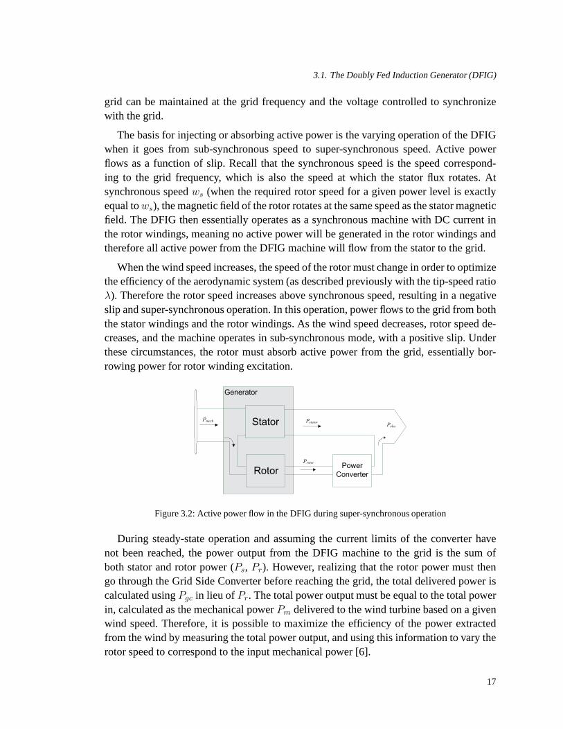
When the wind speed increases, the speed of the rotor must change in order to optimizethe efficiency of the aerodynamic system (as described previously with the tip-speed ratioλ). Therefore the rotor speed increases above synchronous speed, resulting in a negativeslip and super-synchronous operation. In this operation, power flows to the grid from boththe stator windings and the rotor windings. As the wind speeddecreases, rotor speed de-creases, and the machine operates in sub-synchronous mode,with a positive slip. Underthese circumstances, the rotor must absorb active power from the grid, essentially bor-rowing power for rotor winding excitation.
Stator
Generator
RotorPower
Converter
Pelec
Pmech Pstator
Protor
Figure 3.2: Active power flow in the DFIG during super-synchronous operation
During steady-state operation and assuming the current limits of the converter havenot been reached, the power output from the DFIG machine to the grid is the sum ofboth stator and rotor power (Ps, Pr). However, realizing that the rotor power must thengo through the Grid Side Converter before reaching the grid,the total delivered power iscalculated usingPgc in lieu ofPr. The total power output must be equal to the total powerin, calculated as the mechanical powerPm delivered to the wind turbine based on a givenwind speed. Therefore, it is possible to maximize the efficiency of the power extractedfrom the wind by measuring the total power output, and using this information to vary therotor speed to correspond to the input mechanical power [6].
17

Chapter 3. DFIG Detailed Model
Stator
Generator
RotorPower
Converter
PelecPmech Pstator
Protor
Figure 3.3: Active power flow in the DFIG during sub-synchronous operation
3.1.5 DC-link chopper / DC crowbar
A braking resistor is provided in the dc-link bus as a form of protection to dissipate excessenergy during a grid fault. The resistor is connected to the dc-link bus in series with anIGBT, and is referred to as either the dc-link chopper or the dc crowbar. The IGBT cancontrol the amount of energy burned in the resistor, with theresistor (or set of parallelresistors), sized to handle a specific amount of energy during a grid fault. The largerthe fault that is desirable to ride through, the larger the physical size of the resistor orresistors must be. This design decision can be a function of utility requirements for faultride through, as the energy dissipation during a fault is a function of the voltage dipmagnitude and fault duration [7] [6].
3.1.6 AC Crowbar
An AC crowbar is implemented on the rotor side of the RSC, which acts to bypass theRSC by applying a short-circuit to the rotor terminals. Thisacts to protect the RSC fromovercurrents as well as to protect the DC-link from overvoltages. The crowbar can beconstructed by the use of either anti-parallel thryristorsconnected to external resistanceson the rotor phases, or a diode rectifier bridge in series witha single external resistance.When using a diode rectifier bridge, a single thyristor must still be used to control theactivation and deactivation of the crowbar.
The crowbar is an important aspect in not only the protectionof the converter com-ponents, but in understanding the behavior of the DFIG machine during grid faults. Asdescribed, the crowbar acts to protect the rotor-side converter from overcurrents and pro-tect the DC-link from overvoltages. Therefore, the behavior of both the rotor current androtor voltage, as well as the typical setpoints for overcurrent and overvoltage protection,must be understood in order to adequately represent adetailedDFIG model. The amountof detail in the crowbar action that is carried through to anysimplifiedmodels is an im-
18

3.2. 5th Order Machine Model
portant question that is studied in later sections with the derivation of the DFIG simplifiedmodel.
In [6], several common parameters are listed for crowbar activation. For dc-link over-voltage protection, a common setting is at 12% above nominalvoltage. For overcurrentprotection, the converter IGBTs can typically handle twicethe nominal current for a shortduration. Therefore a common overcurrent protection for the converter is set near 1.8pu. These parameters are specific to each converter manufacturer, but may be consideredreasonable assumptions when developing a generic DFIG model.
One interesting aspect of the crowbar action that impacts the DFIG response to gridfaults is the speed at which the crowbar can switch on to dissipate energy and switchoff to return to normal operation mode. A thyristor can only disconnect the current at azero crossing, which, coupled with the issue of fault currents containing dc-components,causes a slight delay on the order of tens of ms [6]. An active crowbar utilizing an IGBTcan be used to force commutation of the rotor current and operate more quickly than thethyristor.
3.2 5th Order Machine Model
The first model of the DFIG that will be developed and analyzedin this thesis is the 5thorder transient model. The model is developed from the basicelectrical circuit equationsthat describe the DFIG machine, including the stator and rotor flux (current) dynamicsand the rotor speed dynamics.
The 5th order model is derived in the synchronous coordinatesystem, also referredto as the d-q coordinate system. The q-axis of the rotating coordinate system is alignedwith the grid voltage, and rotates at the nominal grid frequency of 50 Hz. The alignmentwith the grid voltage allows for simplifications of the circuit equations since the stator isconnected directly to the grid. The q-component of the stator voltage will therefore appearto ”stand still” as it is aligned with the q-axis and rotatingat the same speed. As a result,for a balanced 3-phase system and for balanced 3-phase-to-ground faults,usd = 0.
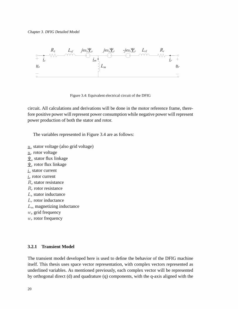
Figure 3.4 represents the equivalent electrical circuit ofthe dynamic DFIG model.This representation is referred to as the T-equivalent circuit, with the stator representedon the left, and the rotor on the right. The interface betweenthe two is represented bythe magnetizing inductanceLm, which also represents the air-gap in the machine and iscommonly referred to as the air-gap flux. The stator terminals are connected directly tothe grid through a step-up transformer, while the rotor is connected to the grid throughback-to-back converters and an interconnection transformer. In this thesis the transformerratios are assumed to be 1:1 for simplicity and are thereforenot shown in the equivalent
19
Chapter 3. DFIG Detailed Model
RS jωsΨs RrLrl
Lm
im
jωsΨr -jωrΨr
us ur
Lsl
iris
Figure 3.4: Equivalent electrical circuit of the DFIG
circuit. All calculations and derivations will be done in the motor reference frame, there-fore positive power will represent power consumption whilenegative power will representpower production of both the stator and rotor.
The variables represented in Figure 3.4 are as follows:
us stator voltage (also grid voltage)ur rotor voltageΨs stator flux linkageΨr rotor flux linkageis stator currentir rotor currentRs stator resistanceRr rotor resistanceLs stator inductanceLr rotor inductanceLm magnetizing inductancews grid frequencywr rotor frequency
3.2.1 Transient Model
The transient model developed here is used to define the behavior of the DFIG machineitself. This thesis uses space vector representation, withcomplex vectors represented asunderlined variables. As mentioned previously, each complex vector will be representedby orthogonal direct (d) and quadrature (q) components, with the q-axis aligned with the
20
3.2. 5th Order Machine Model
stator voltage.
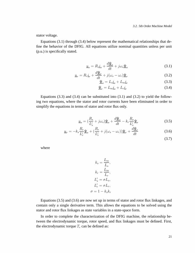
Equations (3.1) through (3.4) below represent the mathematical relationships that de-fine the behavior of the DFIG. All equations utilize nominal quantities unless per unit(p.u.) is specifically stated.
us = Rsis +dΨs
dt+ jωsΨs (3.1)
ur = Rrir +dΨr
dt+ j(ωs − ωr)Ψr (3.2)
Ψs = Lsis + Lmir (3.3)
Ψr = Lmis + Lrir (3.4)
Equations (3.3) and (3.4) can be substituted into (3.1) and (3.2) to yield the follow-ing two equations, where the stator and rotor currents have been eliminated in order tosimplify the equations in terms of stator and rotor flux only.
us = (Rs
L′
s
+ jωs)Ψs +dΨs
dt− kr
Rs
L′
s
Ψr (3.5)
ur = −ksRr
L′
r
Ψs + (Rr
L′
r
+ j(ωs − ωr))Ψr +dΨr
dt(3.6)
(3.7)
where
ks =Lm
Ls
,
kr =Lm
Lr
,
L′
s = σLs,
L′
r = σLr,
σ = 1− kskr
Equations (3.5) and (3.6) are now set up in terms of stator androtor flux linkages, andcontain only a single derivative term. This allows the equations to be solved using thestator and rotor flux linkages as state variables in a state-space form.
In order to complete the characterization of the DFIG machine, the relationship be-tween the electrodynamic torque, rotor speed, and flux linkages must be defined. First,the electrodynamic torqueTe can be defined as:
21

Chapter 3. DFIG Detailed Model
Te =3
2pkr
L′
s
ℑ[Ψ∗
rΨs] =3
2pkr
L′
s
(ΨrdΨsq −ΨrqΨsd) (3.8)
whereℑ is the imaginary part, andp represents the number of machine poles. Therelationship between the electromagnetic torque producedby the machine, the load torquefrom the wind turbineTL, and the rotor speed is defined in what is called the ”swing”equation.
J
p
dωr
dt= Te − TL − b
ωr
p(3.9)
whereJ is the combined inertia of the machine and turbine inkgm2 andb is the speeddependent damping term. This equation demonstrates that any imbalance in the electro-magnetic torqueTe and load torqueTL will result in a change in the rotor speed, eitheracceleration or deceleration, represented asdωr
dt. If Te andTL are equal, as in steady state,
the rotor speed will reach its steady state value and the derivative term will therefore bezero. The swing equation is fundamental in describing and understanding the behavior ofthe DFIG during transient stability studies.
In order to use the swing equation in the state-space form, the equations (3.8) and (3.9)must be combined and described in terms of the state variables, which in this case are theflux linkages and rotor speed. The resulting equation is:
J
p
dωr
dt=
3
2pkr
L′
s
(ΨrdΨsq −ΨrqΨsd)− TL − bωr
p(3.10)
Simulink is used to solve the set of differential equations using the S-function feature.The equations for a state-space formulation are of the form:
x = Ax +Bu
y = Cx +Du
wherex is the state variable vector,y is the output vector,u is the input vector, and vectorsA throughD are vectors defined by the system parameters.
Therefore, with the selected state variables of rotor flux, stator flux, and rotor speed,the derivatives of each (x) are solved for in (3.5), (3.6), and (3.10) to set up the followingstate-space representation of the differential equations:
dΨsd
dtdΨsq
dtdΨrd
dtdΨrq
dtdωr
dt
=
−Rs
L′
sωs kr
Rs
L′
s0 0
−ωs −Rs
L′
s0 kr
Rs
L′
s0
ksRr
L′
r0 −Rr
L′
rωs − ωr 0
0 ksRr
L′
rωr − ωs −Rr
L′
r0
0 3
2
p2
JkrL′
sΨrd 0 −3
2
p2
JkrL′
sΨsd − b
J
Ψsd
Ψsq
Ψrd
Ψrq
ωr
+
22

3.2. 5th Order Machine Model
1 0 0 0 0
0 1 0 0 0
0 0 1 0 0
0 0 0 1 0
0 0 0 0 − p
J
usdusqurdurqTL
(3.11)
With the rotor and stator flux linkages, the rotor and stator currents can be obtainedfrom equations (3.3) and (3.4) as follows:
is =Ψs − krΨr
L′
s
(3.12)
ir =Ψr − ksΨs
L′
r
(3.13)
3.2.2 Γ-equivalent Model
The previous set of equations were derived in order to describe the DFIG machine itself.However, in order to derive the controller for the machine, the T-model of the equivalentcircuit must first be transformed. The T-model contains a unique set of current and fluxlinkages for the stator and rotor side. In order to simplify and consolidate these variables,the stator leakage inductance can be moved to the rotor side,allowing the stator and rotorleakage inductance to be combined. This also allows the stator flux to be expressed interms of the magnetizing inductance and magnetizing current. The resulting circuit isdenoted theΓ-equivalent model. First, the transformation variableb is defined as
b =Ls
Lm
The transformation variable allows the parameters to be transformed from the T-equivalentmodel to theΓ-equivalent model. The following parameters are defined fortheΓ-equivalentmodel, where an uppercase subscript is used to differentiate between the two models.
LM = bLm = Ls
RR = b2Rr
Lσ = bLsl + b2Lrl = b2Lr − Ls
The transformation variableb also allows for the following rotor side equivalent vari-ables for theΓ-model:
23

Chapter 3. DFIG Detailed Model
iR =irb
(3.14)
ΨR = bΨr (3.15)
uR = bur (3.16)
The stator side variables can be transformed starting from the T-model equations. First,the stator flux can be expressed as:
Ψs = Lmir + Lsis
= Ls(Lm
Ls
ir + is)
= Ls(1
bir + is)
= LM(iR + is) (3.17)
The stator voltage can be expressed as:
us = Rsis +dΨs
dt+ jωsΨs
= Rsis +d(LM(ir + is))
dt+ jωsΨs
= Rsis + LM
diMdt
+ jωsΨs (3.18)
The rotor flux for theΓ-model can be expressed as:
ΨR = bΨr
= b(Lrir + Lmis)
= b(biRLr + Lmis)
= b2LriR + LM is
=Lσ + Ls
Lr
LriR + LM is
= LσiR + LsiR + LM is
= LσiR +Ψs (3.19)
Finally the rotor voltage for theΓ-model can be expressed by multiplyingb to the rotorvoltage equation in (3.2):
24

3.3. Control of DFIG Machine
uR = bur
= b(Rrir) + b(dΨr
dt) + b(j(ωs − ωr)Ψr)
= RRiR +dΨR
dt+ j(ωs − ωr)ΨR
= RRiR + Lσ
diRdt
+ LM
diMdt
+ j(ωs − ωr)ΨR (3.20)
Equations (3.18) and (3.20) can be used to set up theΓ-equivalent model as shown inFigure 3.5. TheseΓ-model equations will be used moving forward with the designof thevarious controllers.
RS jωsΨs RRLσ
LM
iM
jωsΨR -jωrΨR
us uR
iRis
Figure 3.5:Γ-Equivalent electrical circuit of the DFIG, showing statorand rotor leakage inductance com-bined and allowing stator flux to be expressed in terms of magnetizing inductance and current.
3.3 Control of DFIG Machine
3.3.1 Rotor Current Controller
The rotor current controller controls the rotor current by calculating the required rotorvoltage needed for a given reference current value. Therefore, the current controller mustfirst define a system model of the DFIG machine, which can be done by deriving a transferfunction fromuR to iR. This can be accomplished by solving foruR
iRfrom the previously
derived equations describing the machine. First, the rotorvoltage equation is transformedto eliminateiM by solving equation (3.18) forLM
diMdt
and inserting into equation (3.20)as follows:
uR = RRiR + Lσ
diRdt
+ (us − Rsis − jωsΨs) + j(ωs − ωr)ΨR
25

Chapter 3. DFIG Detailed Model
Next, both the stator currentis and rotor fluxΨR are eliminated:
uR = RRiR + Lσ
diRdt
+ us −Rs(Ψs
LM
− iR)− jωsΨs + j(ωs − ωr)(LσiR +Ψs)
= us + Lσ
diRdt
+ (Rs +RR)iR + j(ωs − ωr)LσiR − Rs
LM
Ψs − jωrΨs (3.21)
By taking the Laplace transform of equation (3.21), the rotor voltage equation resultsin the following:
uR = us + iR(Rs +RR + sLσ) + j(ωs − ωr)LσiR − Rs
LM
Ψs − jωrΨs (3.22)
where the term( Rs
LM+ jωr)Ψs is defined as the back EMF of the machine (E). As
mentioned, it is desired to solve for the transfer function from uR to iR, which can bedone by solving foruR
iR. As this cannot be done directly, the stator voltageus and machine
back EMFE can be treated as disturbances, resulting in the following transfer function:
GC =iR
(uR − us + E)=
1
sLσ +Rs +RR + j(ωs − ωr)Lσ
(3.23)
For the derivation of the controller, the termj(ωs − ωr)Lσ can be treated with a feedforward loop. The transfer functionGC is therefore reduced to simply:
GC =1
(sLσ +Rs +RR)(3.24)
There are several methods in which a controller can be designed. The method thatwill used in this thesis is internal model control (IMC). IMCsimply uses the knowledgeof the system model to develop the control parameters required to augment the errorbetween the actual system and the model of the system. The controller can be derivedfrom the following relationship, whereF (s) represents the controller transfer function,and knowing that the control loop should behave like a first-order transfer function.
F (s)G(s)
1 + F (s)G(s)=
α
s+ α
F (s)G(s) =α
s
F (s) =α
s(sLσ +Rs +RR) (3.25)
26

3.3. Control of DFIG Machine
For a PI controller,F (s) can be set equal tokp +kis
, and the PI controller parametersderived as follows:
F (s) =α
s(sLσ +Rs +RR) = kpc +
kic
s
= αLσ + α(Rs +RR)
s= kpc +
kic
s(3.26)
and therefore
kpc = αLσ (3.27)
kic = α(Rs +RR) (3.28)
With these control parameters, and using equation (3.22), the reference values for therotor voltage can be obtained from the following equations:
urefRd = (kpc +
kic
s)(irefRd − iRd) + usd − (ωs − ωr)LσiRq
− Rs
LM
Ψsd + ωrΨsq (3.29)
urefRq = (kpc +
kic
s)(irefRq − iRq) + usq + (ωs − ωr)LσiRd
− Rs
LM
Ψsq − ωrΨsd (3.30)
3.3.2 Active DampingRa
An additional term can be included in the design of the current controller, called ”activeresistance”, orRa. The active resistance is added to the actual machine resistance valuesin the transfer function, and gives additional flexibility in damping out variations of theback emf. This resistance is not ”real” in the sense that it isnot physically present in themachine, but is added purely for a higher level of control. When introducing an activeresistance, the controller gains must be updated to accountfor Ra. The new controllergains are
kpc = αLσ (3.31)
kic = α(Rs +RR +Ra) (3.32)
27

Chapter 3. DFIG Detailed Model
3.3.3 Rotor Current Reference Calculation
The reference values for the rotor current can be derived directly from the equations thatdescribe the electrodynamic torque of the machine and the stator reactive power.
q-axis rotor current reference calculation
First, the equation for the electrodynamic torque is revised to include the rotor current. Itis important to note that there are several ways in which the electrodynamic torque can beexpressed, and throughout the literature on this topic a variety of forms of the equationare presented. It can be shown algebraically that these equations are all equivalent. Thefollowing is the equation used for the purposes of deriving the rotor current referencevalues.
Te = −3
2pℑ[Ψ∗
siR]
= −3
2pℑ[(Ψsd − jΨsq)(iRd + jiRq]
= −3
2p(ΨsdiRq −ΨsqiRd) (3.33)
As was discussed previously, the d-q coordinate system for this thesis has aligned thestator voltage with the q-axis. Therefore,usd = 0. Equation (3.18), which describes thestator voltage for theΓ-model, can be used to simplify equation (3.33). With the assump-tions thatRs = 0 (Rs is in fact a very small value), and that the machine operates insteady-state (which allows the derivative term to be set equal to 0), thenΨsq = 0. Since itis difficult to measure the torque, it is often commonly controlled with an open loop [5].Equation (3.33) can then be simplified to yield the equation for the q-axis rotor currentreference value.
Te = −3
2p(ΨsdiRq)
irefRq = − 2
3p
T refe
Ψsd
(3.34)
The simplifications and assumptions used to deriveirefRq do have an impact on the con-
trollability of the torque. TheirefRq that is fed into the current controller in order to achievethe reference torque value is not accurate because it does not take into account the statorresistance. Therefore, the actual torque of the machine will always differ from the refer-ence torque, resulting in a steady-state error. If the mechanical torqueTm is set equal to
28

3.3. Control of DFIG Machine
the reference torqueT refe , as is common to do, the steady state difference between the
two will result in a continuous increase or decrease of the rotor speed due to the swingequation defined in equation (3.9). This can be corrected with a speed controller in cas-cade with the current controller that is used to adjustT ref
e in order to keep the rotor speedconstant. Another alternative is to use an active power controller to deriveirefRq . These twooptions are elaborated in the following sections.
d-axis rotor current reference calculation
The d-axis rotor current reference value can be derived froman understanding of the statorreactive power.irefRd is derived as follows:
Qs =3
2ℑ[usi∗s]
=3
2ℑ[(Rsis + LM
diMdt
+ jωsΨs)(Ψs
LM
− iR)∗]
and assumingRs = 0 and steady state conditions, simplifies to
Qs =3
2ℑ[jωsΨs)(
Ψs
LM
− iR)∗]
=3
2usq(
Ψsd
LM
− iRd) (3.35)
Equation (3.35) can be used directly to solve for theirefRd value.
irefRd =
Ψsd
LM
− 2
3
Qrefs
usq(3.36)
The equation (3.36) represents control ofirefRd in an open loop manner. The following
section expands on usingQs to controliRd in a closed-loop control system.
3.3.4 Reactive Power (Q) Controller
For the DFIG machine in a wind turbine application, it is desirable to control the re-active power. In steady-state, the controller should keep the reactive power set equal tozero, therefore maximizing the active power injection to the grid. During a fault condi-tion where the grid voltage drops, it may be desirable to inject reactive power from theDFIG in order to provide voltage support. The magnitude and duration of reactive power
29
Chapter 3. DFIG Detailed Model
injection is dependent on the requirements of the local gridcodes, to be explained in moredetail later in this thesis.
The DFIG has two connections to the grid, allowing for reactive power injection andconsumption to be controlled through either the rotor or stator circuit. In practice, the GSCin the rotor circuit always controls the reactive power to zero. The RSC in the rotor circuitcan be used to control the stator reactive power by controlling irefRd , and it is through thecontrol ofirefRd that the DFIG is able to provide reactive power support during grid voltagedips. Equation (3.35) can be used to derive the reactive power controller parameters.
First, the transfer functionGQ fromQs to iRd can be defined as
GQ =Qs
iRd − Ψsd
LM
= −3
2usq (3.37)
The controllerFQ(s) can be defined using internal model control as was shown inequation (3.25) to yield the following relationship
FQ(s) =αQ
sG−1
Q (s) = −2αQ
3usq
1
s(3.38)
In deriving the controller it is shown that only an I-controller is needed using the in-ternal model control method. The gain of the controllerkiQ = − 2αQ
3usq. In this thesis, the Q
controller is implemented with an I-controller only with a bandwidth initially set to 100rad/s (10 times slower than the initial setting of the current controller bandwidth).
For this thesis, during steady state and normal operation, the reactive power output ofthe DFIG machine will be set to zero (Qgc = Qs = 0), and the machine will prioritizeactive power output. During voltage dips, all models will implement the E.ON grid codereactive power requirement as previously described. This requires reactive power to besupplied by the DFIG machine for all voltage dips less than 0.9 p.u., and is a function ofthe severity of the voltage dip. This acts to prioritize reactive power output during voltagedips, and only provide real power if there is sufficient capacity left without exceeding therotor current limitations.
3.3.5 Speed Controller
A speed controller can be used in cascade with the current controller to control the rotorspeed to a constant steady-state value. The rotor speed reference value can be obtainedbased on the power-speed relationship of the wind turbine, typically in the form of atable. This table shows the relationship of rotor speed on the input mechanical power (ormechanical torque). The actual rotor speed can thus be measured and compared to the
30

3.3. Control of DFIG Machine
reference value, with the controller giving a torque reference that is fed into the currentcontroller.
The rotor speed dynamics are reasonably slow when compared to the time of a voltagedip event. Voltage dips commonly last less than one second. This thesis analyzed the rotorspeed dynamics during the voltage dip to determine if an assumption of a fixed rotor speedis valid for transient stability and voltage stability studies.
In this thesis, a speed controller was implemented in one of the detailed model it-erations for the purposes of comparison and to analyze the impact to the results. Thecontroller was derived using internal model control, usingthe swing equation of
J
p
dωr
dt= Te − TL − Bωr (3.39)
whereB is the speed dependent damping term. In this equation,Te is set equal toT refe
and the load torqueTL is treated as a disturbance. Therefore, the transfer functionGω(s)
can be found by taking the Laplace transform and solving for the ratio ofT refe to ωr,
resulting in the following equation
Gω =T refe
ωr
=J
ps+B (3.40)
yielding the following controller equation
Fω(s) =αω
sG−1
ω (s) = αω
J
p+ αω
B
s(3.41)
The controller parameters can be taken directly from (3.41)askp = αωJp
andki =
αωB. The speed controller bandwidth for this thesis was set to beslower than the innerloop control at100 rad
s.
When using a speed controller, considerations must be takenregarding high versuslow wind speeds. During low wind speeds, before the wind turbine has reached ratedpower output, each wind speed corresponds to a unique power value. However, when thewind speed increases and the wind turbine reaches rated power, the wind speed is used tocontrol the pitch and not the power. This results in two controllers that are dependent onthe wind speed - one controller that gives a torque or power reference (low wind speeds),and one controller that gives a pitch reference (high wind speeds). The controller mustswitch between the two modes dependent on the wind speed.
31

Chapter 3. DFIG Detailed Model
3.3.6 Active Power (P) Controller
An active power controller can also be used in cascade with the current controller in lieuof the speed controller. In this case, the reference power value is obtained from the windturbine’s power-speed relationship, representing the mechanical power into the machine.This value is compared to the actual active power output, which is calculated from thesum of the stator power (Ps) and the grid-side converter power (PGC).
For the purposes of this thesis, a simulation is performed for one operating point at atime. For example, the wind turbines may be modeled at rated power for a given voltagedip to study the effects of voltage and transient stability on the system. The simulationdoes not dynamically change between operating points. For this reason, when operatingat just one operating point, an active power controller may be considered equivalent toa speed controller. The advantage of using an active power controller is that it is notnecessary to switch between control modes for high and low wind speeds. The model canbe used for the full range of operation. For this reason, a P controller is used for outerloop control in lieu of a speed controller.
The power controller was derived using internal model control using the torque rela-tionship of (3.33) and the relationship between power and torque as follows
irefRq = − 2
3p
T refe
Ψsd
(3.42)
andP = TΩ (3.43)
yield the transfer functionGP (s) of
GP =Pref
iRq
= −3
2pΨsdΩ (3.44)
yielding the following controllerFP (s)
FP (s) =αp
sG−1
p (s) = −αp
s
2
3pΨsdΩ(3.45)
This results in an integrator only controller. By substituting Ω = ωr
p, and realizing
the steady state relationship ofΨsd = usq
ωs, the integrator parameterki can be found as
− 2ωs
3usqωr.
32
Chapter 4
Converter limitations and modelimplementation of DC-chopper
The rotor-side converter and grid-side converter have physical limitations that must beaccounted for in the model. It is typical to have the converters in a DFIG wind turbinesystem sized at around 30% of the rated power of the generator. The limitation is realizedin the form of both voltage and current limitations. A full model of these limitationswould require implementation of a DC-link controller to properly model the DC-linkvoltage during transients. The control of DC-link voltage impacts the action of the DCcrowbar used to release energy and protect the DC-link from overvoltage. As the intent ofthis thesis is to develop a simplified model for implementation in PSS/E, the DC-choppercontroller is considered to act instantaneously with respect to the time step of the PSS/Esimulation and is therefore not implemented in this thesis.
This section will describe how the voltage and current limitations on the rotor circuitare modeled in this thesis. It will also describe the operation of the DC-chopper, and howthe DC-chopper was implemented in the detailed model.
4.1 Rotor voltage limitation
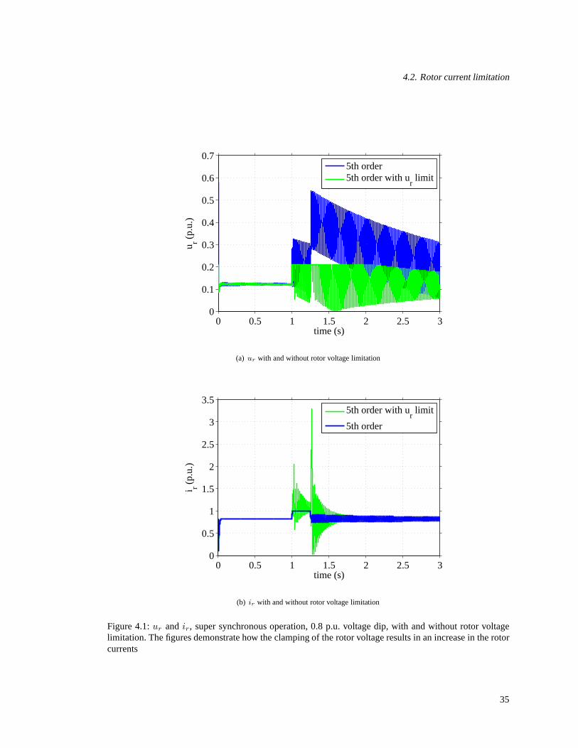
The RSC controls the rotor voltageuR to obtain the desired currentiR required to controlthe torque and reactive power of the machine. If under certain conditions, the rotor voltagerequired to meet these demands is increased beyond a certainthreshold, the converter willclamp the voltage and limit it to this amount. In this thesis,the maximum rotor voltagewas determined based on the analysis of the 2MW wind turbine done in the Tvaaker report[8]. The result of clamping the voltage causes higher rotor currents. This is illustrated infigures 4.1 through 4.4 below. The basic 5th order machine model with P and Q controllers
33

Chapter 4. Converter limitations and model implementationof DC-chopper
is compared to the same model but with a rotor voltage limitation. The actual limit of therotor voltage is determined by the relationship with the DC-link voltage. This relationshipwill be described in more detail in the subsequent section.
Due to the poorly damped poles, the oscillations experienced during voltage dips arevery high. The rotor currents exceed the maximum current by alarge amount and causethe RSC to operate at maximum voltage for an extended period of time. This affects theability of the RSC to control theP andQ output.
4.2 Rotor current limitation
DC
Chopper
DC-link
capacitor
Rotor-side
converter
Rotor
terminals
Figure 4.5: Rotor-side converter with DC-link
In a fully detailed model with a DC-link controller, the activation of the DC-chopper canbe modeled by first monitoring the DC-link voltage. Refer to figure 4.5 for a represen-tation of the RSC with DC-link. During a grid fault, there is aquick drop in the statorvoltage. This causes an increase in the stator current (because of the controller’s attemptto maintain the reference power output), which causes an increase in the rotor current. Ifthe newir can be achieved, then the power output remains unchanged. However if thenewir cannot be achieved, thenPs will decrease andPr will increase.
When higher rotor currents are required, the RSC attempts toincrease the rotor voltageapplied to the rotor circuit. This will work until the applied voltage reaches the maximumlimit, which forces the RSC to clamp the voltage. However, byclamping the rotor voltage,the rotor circuit will experience an increase in the rotor current. Eventually a high rotorcurrent will exceed the limit of the IGBT’s in the RSC, and theRSC will subsequentlysend a turn-off signal to the IGBT’s resulting in current flowthrough the freewheelingdiodes. When this occurs, the RSC has lost controllability of the rotor circuit voltage, and
34
4.2. Rotor current limitation
0 0.5 1 1.5 2 2.5 30
0.1
0.2
0.3
0.4
0.5
0.6
0.7
time (s)
u r (p.
u.)
5th order5th order with u
r limit
(a) ur with and without rotor voltage limitation
0 0.5 1 1.5 2 2.5 30
0.5
1
1.5
2
2.5
3
3.5
time (s)
i r (p.
u.)
5th order with ur limit
5th order
(b) ir with and without rotor voltage limitation
Figure 4.1:ur and ir, super synchronous operation, 0.8 p.u. voltage dip, with and without rotor voltagelimitation. The figures demonstrate how the clamping of the rotor voltage results in an increase in the rotorcurrents
35
Chapter 4. Converter limitations and model implementationof DC-chopper
0 0.5 1 1.5 2 2.5 3−1
0
1
2
3
4
5
time (s)
P tota
l (p.
u.)
5th order with ur limit
5th order
(a) Ptotal with and without rotor voltage limitation
0 0.5 1 1.5 2 2.5 3−1.5
−1
−0.5
0
0.5
1
1.5
2
time (s)
Qs (
p.u.
)
5th order with ur limit
5th order
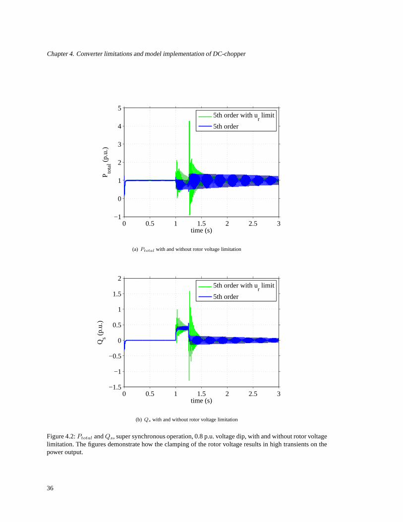
(b) Qs with and without rotor voltage limitation
Figure 4.2:Ptotal andQs, super synchronous operation, 0.8 p.u. voltage dip, with and without rotor voltagelimitation. The figures demonstrate how the clamping of the rotor voltage results in high transients on thepower output.
36

4.2. Rotor current limitation
0 0.5 1 1.5 2 2.5 30
0.5
1
1.5
2
time (s)
u r (p.
u.)
5th order5th order with u
r limit
(a) ur with and without rotor voltage limitation
0 0.5 1 1.5 2 2.5 30
1
2
3
4
5
6
7
time (s)
i r (p.
u.)
5th order with ur limit
5th order
(b) ir with and without rotor voltage limitation
Figure 4.3:ur andir, super synchronous operation, 0.25 p.u. voltage dip, with and without rotor voltagelimitation. The figures demonstrate how the clamping of the rotor voltage results in an increase in the rotorcurrents
37
Chapter 4. Converter limitations and model implementationof DC-chopper
0 0.5 1 1.5 2 2.5 3−4
−2
0
2
4
6
8
time (s)
P tota
l (p.
u.)
5th order with ur limit
5th order
(a) Ptotal with and without rotor voltage limitation
0 0.5 1 1.5 2 2.5 3−8
−6
−4
−2
0
2
4
time (s)
Qs (
p.u.
)
5th order with ur limit
5th order
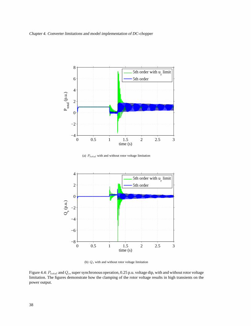
(b) Qs with and without rotor voltage limitation
Figure 4.4:Ptotal andQs, super synchronous operation, 0.25 p.u. voltage dip, with and without rotor voltagelimitation. The figures demonstrate how the clamping of the rotor voltage results in high transients on thepower output.
38

4.3. Grid-side converter current limitation
has become a diode rectifier. The rotor current will begin to charge the DC-link capacitorand cause an increase to the DC-link voltage. WhenUdc > 1.12p.u., the DC-chopper isactivated to release energy through the DC-chopper resistor. Refer to figure 4.6.
Rotor
terminals
idc
Rdc
idc
1.12*Udc
Figure 4.6: Rotor-side converter with DC-link
The DFIG can still be described by the same equations as before, however the rotorvoltage magnitude is now determined by the DC-link voltage alone. The phase angle ofthe rotor voltage is equal to the phase angle of the rotor current, since the crowbar is apure resistor (power factor= 1.0). The rotor voltage magnitude can be described withthe following equation representing the relationship between phase voltage and DC-linkvoltage of a diode rectifier [9].
uR,phase =Udcπ
3√3
(4.1)
The equation used to derive the rotor voltage during diode rectification is based ona diode rectifier with a current stiff DC source. For the case of the RSC and DC-linkused in this thesis, it is more appropriate to consider the system with a constant DC-sidevoltage. However it is shown in [9] that this voltage relationship can still be used as anapproximation.
4.3 Grid-side converter current limitation
Similar to the RSC, the GSC is limited based on the rating of the converter components.As discussed previously, the rotor circuit is designed to withstand around 30% of therated generator power. This value is determined by the allowable range of the rotor speedaround synchronous speed, as this determines the slip powerand thus the power flowingthrough the rotor circuit.
The grid side converter active power can be calculated with:
Pgc = 1.5(ugcdigcd + ugcqigcq) (4.2)
39

Chapter 4. Converter limitations and model implementationof DC-chopper
The voltageugc is set equal to the grid voltage, therefore:
ugcd = usd = 0
ugcq = usq
yielding the final equation forPgc as:
Pgc = 1.5Ngsusqigcq) (4.3)
whereNgs represents the turns ratio of the transformer between the GSC and the stator.In this thesis, all transformers are modeled with a turns ratio equal to 1.
Similarly, the grid side converter reactive power can be calculated as:
Qgc = 1.5(ugcqigcd − ugcdigcq)
= 1.5(ugcqigcd)
= 1.5Ngsusqigcd (4.4)
This allows for the equations describing the dq grid side converter currents as:
igcd =Qgc
1.5Ngsusq(4.5)
igcq =Pgc
1.5Ngsusq(4.6)
The total GSC current|igc| is limited by the GSC to a certain value,igc,max. In thisthesis, the sizing of the VSCs is based on their ability to handle 30% of the rated generatorpower. Therefore, the maximum GSC current is set to 0.3 p.u.
The active power that flows through the RSC must also flow through the GSC beforereaching the grid. Therefore in the calculation of the GSC current,Pgc can be set equal toPr, as long as the resulting GSC current does not exceed the maximum value. The reactivepower is typically controlled to be zero, thereforeQgc = 0.
4.4 Model implementation of DC-chopper
The main goal of implementing the DC-chopper in the 5th orderdetailed model is tounderstand the effects of the DC-chopper action on the overall energy balance and energy
40

4.4. Model implementation of DC-chopper
transfer of the machine and the grid. Since the end goal of this model is to simplify itfor use as a positive sequence model for modeling active and reactive power during gridfaults, it is not necessary to simulate the actual power consumed by the DC-chopper orthe variations in the DC-link voltage during the chopper action, as long as the interchangeof power with the grid is properly represented.
The approach taken to calculateur during crowbar operation was to look at the stepstaken by the RSC when moving from the controllable range to DC-chopper operation.
• The VSC output reaches its maximum value (ur,max)
• The RSC will lose control instantaneously when|ir| > ir,max
• When the RSC loses controllability, the rotor voltage magnitude will be locked tothe maximum rotor voltage, as derived from equation (4.1) based on the nominalDC-link voltage
• When the RSC loses controllability, the rotor voltage phaseangle will be set equalto the rotor current phase angle
• The loss of RSC control signifies the switch to a diode rectifier, and thus the changein rotor voltage. Any excess energy caused by a difference inthe rotor active powerand grid-side active power is assumed to be burned in the DC crowbar resistor.
Therefore, to analyze the effects of the DC-chopper operation, the model implementsa switch that changes the rotor voltage based on the operation of a diode rectifier. Theswitch is activated when the rotor current exceeds its maximum value. The rotor voltagemagnitude is fixed at the maximum value as determined by the DC-link voltage (equation(4.1)), and the rotor voltage angle is switched to be in phasewith the rotor current. Basedon the use of the motor convention in this thesis, where positive power is going into themachine, the rotor voltage must actually be 180 degrees out of phase with the rotor cur-rent to simulate active power going from the machine to the DC-link during diode rectifieroperation. For the purposes of this discussion, this model will be described as though theRSC maintains control throughout since it incorporates thebase current controller only(without consideration of what happens when the current limitation is reached). This as-sumption is not entirely true as the current controller cannot achieve the desired referencerotor voltage during saturation.
Figure 4.7 shows a comparison of the model with the diode rectifier implemented, andwithout the diode rectifier implemented (5th order model with rotor voltage limitation),when applying a voltage dip of 0.8 p.u.. It can be seen in this figure that the rotor currentdecreases more quickly during the fault when the diode rectifier is implemented. Thefigure also shows how the rotor voltage magnitude remains clamped during diode rectifier
41

Chapter 4. Converter limitations and model implementationof DC-chopper
operation. Figure 4.8 shows a comparison ofPtotal andQ with and without the dioderectifier implemented. In figure 4.9, a deep voltage dip of 0.25 p.u. was applied for supersynchronous operation (full power operation), and the resulting effects ofP andQ shown.As with the shallow voltage dip, theP andQ responses are similar between the twomodels.
In summary, the responses inP andQ for the model including the diode rectifier arein good agreement with the model without the diode rectifier.Therefore, moving forwardwith model simplifications, the DC-chopper implementationwill not be included in themodel.
4.4.1 Regaining control of the RSC
In the previously described representation of the DFIG, theRSC loses control and changesto a diode rectifier purely based on the magnitude ofir. The converter switches back andforth between being in control and losing control based on the inequality|ir| ≤ ir,max.However, it is of interest to investigate an alternative method to regaining control of theRSC by studying the rotor voltage when the RSC has lost control and is in diode rectifiermode. To do this, the rotor voltage reference is calculated by the current controller andthen applied to a separate machine model in parallel with themodel implementing thediode rectifier. Recall that this calculated reference rotor voltage will not be the same asthe rotor voltage in the diode rectifier model, as the diode rectifier model will force thereference rotor voltage to be in phase with the rotor current. The resulting rotor currentfrom the parallel model is analyzed to determine if the reference rotor voltage would resultin a rotor current that does not exceed the maximum limit. In other words, the idea is toinvestigate what the rotor voltage would be if the RSC were toregain control, based onthe current states of the system, and see what the resulting rotor current would be if thisnew rotor voltage were applied. This analysis would show thepossibility of switchingbackout of diode rectifier mode and regaining control of the machine more quickly.
Figure 4.10 represents the magnitude of the rotor current for two different scenar-ios. The first scenario is simply the present model with the diode rectifier implemented.Therefore the RSC loses control and switches to a diode rectifier when the rotor currentexceeds its maximum value. The second scenario is a representation of what the rotorcurrent would be if the RSC were to regain control and apply the corresponding rotorvoltage. The area of interest is any location where the rotorcurrent from the controlledscenario dips below the maximum rotor current value (in thisfigure the value is 1.0 p.u.).When the rotor current goes below 1.0 p.u., it is of interest to see if the RSC is in controlor out of control at that time instant. If it is not in control,there is an opportunity to regaincontrol more quickly than by waiting for the rotor current todrop below the maximumlimit.
42

4.4. Model implementation of DC-chopper
0 0.5 1 1.5 2 2.5 30
0.5
1
1.5
2
2.5
3
3.5
time (s)
i r (p.
u.)
5th order with ur limit
5th order with diode rectifier
(a) ir with and without diode rectifier implemented
0 0.5 1 1.5 2 2.5 30
0.05
0.1
0.15
0.2
0.25
time (s)
u r (p.
u.)
5th order with diode rectifier5th order with u
r limit
(b) ur with and without diode rectifier implemented
Figure 4.7:ir andur with and without diode rectifier implemented, for super synchronous operation, 0.8p.u. voltage dip.
43
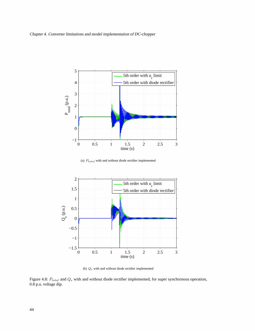
Chapter 4. Converter limitations and model implementationof DC-chopper
0 0.5 1 1.5 2 2.5 3−1
0
1
2
3
4
5
time (s)
P tota
l (p.
u.)
5th order with ur limit
5th order with diode rectifier
(a) Ptotal with and without diode rectifier implemented
0 0.5 1 1.5 2 2.5 3−1.5
−1
−0.5
0
0.5
1
1.5
2
time (s)
Qs (
p.u.
)
5th order with ur limit
5th order with diode rectifier
(b) Qs with and without diode rectifier implemented
Figure 4.8:Ptotal andQs with and without diode rectifier implemented, for super synchronous operation,0.8 p.u. voltage dip.
44

4.4. Model implementation of DC-chopper
0 0.5 1 1.5 2 2.5 3−4
−2
0
2
4
6
8
time (s)
P tota
l (p.
u.)
5th order with ur limit
5th order with diode rectifier
(a) Ptotal with and without diode rectifier implemented
0 0.5 1 1.5 2 2.5 3−10
−8
−6
−4
−2
0
2
4
time (s)
Qs (
p.u.
)
5th order with ur limit
5th order with diode rectifier
(b) Qs with and without diode rectifier implemented
Figure 4.9:Ptotal andQs with and without diode rectifier implemented, for super synchronous operation,0.25 p.u. voltage dip.
45

Chapter 4. Converter limitations and model implementationof DC-chopper
0 0.5 1 1.5 2 2.5 30
1
2
3
4
5
6
time (s)
Rot
or C
urre
nt(p
.u.)
ir,actual
ir,RSC control
(a) The actualir with diode rectifier implemented, andir if the RSC wasin control at all times.
1 1.05 1.1 1.15 1.20
0.5
1
1.5
2
2.5
3
3.5
time (s)
Rot
or C
urre
nt(p
.u.)
ir,actual
ir,RSC control
(b) Enlarged view.
Figure 4.10: The actualir andir that could be achieved if the RSC was in control. The switching betweencontrol mode and diode rectifier mode is represented by the black dashed line. As can be seen, the switchingoccurs whenir decreases below 1.0 p.u.
46
Chapter 5
Evaluation of 5th Order Model againstPSCAD Detailed Model
In an effort to validate the detailed model derived in this thesis, the model was comparedagainst a more detailed model developed in PSCAD. This PSCADmodel has been vali-dated against the field measurements of an actual DFIG wind turbine subject to both anunbalanced shallow voltage dip and a more severe voltage dipwhere the voltage droppedto zero for a period of 70 ms. The PSCAD model showed excellentagreement with thefield measurements [1].
The PSCAD model contains the following design features:
• Full converter PWM switching
• Grid side filter
• DC-link controller, for control of the DC link voltage
• Grid-side converter controller
• Both the P and Q controllers implemented as PI controllers
• Current controller implemented as a P controller only
• A slow rotor speed controller (10 rad/s) to ensure steady-state speed prior to voltagedip
• DC-chopper set to act on DC-link overvoltage
The detailed model was synchronized to the PSCAD model by thefollowing actions:
• Synchronization of machine parameters
47
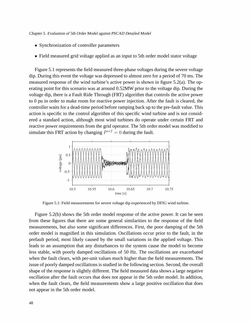
Chapter 5. Evaluation of 5th Order Model against PSCAD Detailed Model
• Synchronization of controller parameters
• Field measured grid voltage applied as an input to 5th order model stator voltage
Figure 5.1 represents the field measured three-phase voltages during the severe voltagedip. During this event the voltage was depressed to almost zero for a period of 70 ms. Themeasured response of the wind turbine’s active power is shown in figure 5.2(a). The op-erating point for this scenario was at around 0.52MW prior tothe voltage dip. During thevoltage dip, there is a Fault Ride Through (FRT) algorithm that controls the active powerto 0 pu in order to make room for reactive power injection. After the fault is cleared, thecontroller waits for a dead-time period before ramping backup to the pre-fault value. Thisaction is specific to the control algorithm of this specific wind turbine and is not consid-ered a standard action, although most wind turbines do operate under certain FRT andreactive power requirements from the grid operator. The 5thorder model was modified tosimulate this FRT action by changingP ref = 0 during the fault.
Figure 5.1: Field measurements for severe voltage dip experienced by DFIG wind turbine.
Figure 5.2(b) shows the 5th order model response of the active power. It can be seenfrom these figures that there are some general similarities to the response of the fieldmeasurements, but also some significant differences. First, the poor damping of the 5thorder model is magnified in this simulation. Oscillations occur prior to the fault, in theprefault period, most likely caused by the small variationsin the applied voltage. Thisleads to an assumption that any disturbances to the system cause the model to becomeless stable, with poorly damped oscillations of 50 Hz. The oscillations are exacerbatedwhen the fault clears, with per-unit values much higher thanthe field measurements. Theissue of poorly damped oscillations is studied in the following section. Second, the overallshape of the response is slightly different. The field measured data shows a large negativeoscillation after the fault occurs that does not appear in the 5th order model. In addition,when the fault clears, the field measurements show a large positive oscillation that doesnot appear in the 5th order model.
48

(a) Measured active power during severe voltage dip.
3 3.05 3.1 3.15 3.2 3.25 3.3
−1
−0.5
0
0.5
1
time (s)
Tot
al A
ctiv
e P
ower
(p.
u.)
(b) Simulated active power during severe voltage dip.
Figure 5.2: Measured and simulatedPtotal for severe voltage dip.
49

Chapter 5. Evaluation of 5th Order Model against PSCAD Detailed Model
In summary, while the general response of the detailed modelagrees with the fieldmeasured response, more research is required to fully validate the detailed model and isincluded as an area for future work.
5.1 Damping analysis of the DFIG model
In [5], the stability of the DFIG is analyzed. It is noted thatin studying the stability of theDFIG mathematically, it can be shown that the DFIG has poorlydamped poles around theline frequency, and also that the system becomes unstable when thed component of therotor current exceeds a certain value. Different methods for damping the flux oscillationsare discussed, and it is noted that a comparison is done in [10]. The methods discussedare:
• feedback of the derivative of the flux. This method was shown to work consider-ably well and at a low cost. The disadvantage concluded from [10] is that it causesrelatively high rotor currents.
• introduce a converter connected to the star point of the stator windings, therebyintroducing an extra degree of freedom that can be used to damp the flux oscillations.This method works quite well, but has the obvious disadvantage of added hardware,software, and thereby added cost.
• reducing bandwidth of the current controller. This method was shown to work quitewell, but compromises the controller’s ability to quickly react to grid disturbances,such as voltage drops or overvoltages.
• compensation of the transformation angle to synchronous coordinates. This methodwas shown to have only a small effect on damping the oscillations.
In this thesis, the DFIG was first modeled without any form of flux damping, followed byan analysis of the poles to determine how best to influence thestability and damping ofthe system.
Initial simulation results of the DFIG with a current controller in cascade with ac-tive power and reactive power controllers show large oscillations close to 50 Hz that aredifficult to damp. An analysis was carried out to define the poles that exist due to the in-teraction between the DFIG machine and current controller.From this analysis, it is madeclear the origin of the poles and which parameters influence the poles, leading to a betterunderstanding of how the poles can be damped.
First, the equations of the machine and current controller were developed and statevariables identified to allow for state-space implementation. This was done in a similar
50
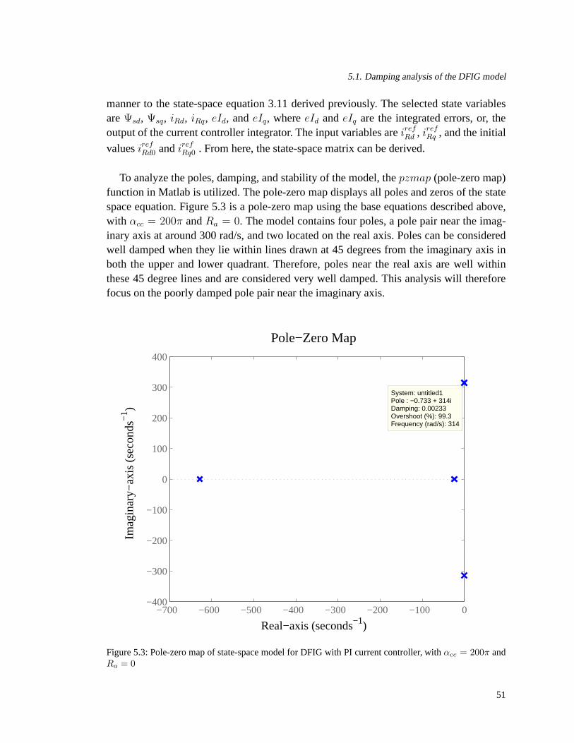
5.1. Damping analysis of the DFIG model
manner to the state-space equation 3.11 derived previously. The selected state variablesareΨsd, Ψsq, iRd, iRq, eId, andeIq, whereeId andeIq are the integrated errors, or, theoutput of the current controller integrator. The input variables areirefRd , irefRq , and the initial
valuesirefRd0 andirefRq0 . From here, the state-space matrix can be derived.
To analyze the poles, damping, and stability of the model, thepzmap (pole-zero map)function in Matlab is utilized. The pole-zero map displays all poles and zeros of the statespace equation. Figure 5.3 is a pole-zero map using the base equations described above,with αcc = 200π andRa = 0. The model contains four poles, a pole pair near the imag-inary axis at around 300 rad/s, and two located on the real axis. Poles can be consideredwell damped when they lie within lines drawn at 45 degrees from the imaginary axis inboth the upper and lower quadrant. Therefore, poles near thereal axis are well withinthese 45 degree lines and are considered very well damped. This analysis will thereforefocus on the poorly damped pole pair near the imaginary axis.
Pole−Zero Map
Real−axis (seconds−1)
Imag
inar
y−ax
is (
seco
nds
−1 )
−700 −600 −500 −400 −300 −200 −100 0−400
−300
−200
−100
0
100
200
300
400
System: untitled1Pole : −0.733 + 314iDamping: 0.00233Overshoot (%): 99.3Frequency (rad/s): 314
Figure 5.3: Pole-zero map of state-space model for DFIG withPI current controller, withαcc = 200π andRa = 0
51

Chapter 5. Evaluation of 5th Order Model against PSCAD Detailed Model
The two poles at 300 rad/s near the imaginary axis represent the poorly damped polesnear 50 Hz that were expected based on the simulation resultsof the detailed DFIG model.A closer inspection reveals a damping coefficient of 0.00233for the two poles. It is desir-able to move these poles off of the imaginary axis, in the direction of the 45 degree linesthat represent well damped poles. With this understanding,the DFIG model parameterscan now be modified to see how or if the poles can be moved to increase the damping.The following cases were analyzed:
• With and without the back emf feed forward term
• With and without the active damping termRa
• Varying values of stator resistanceRs
• Varying values of rotor resistanceRR
• Varying values of magnetizing inductanceLM
• Varying values of stator inductanceLs
• Varying values of stator voltage magnitudeUs
• Varying values of rotor speedωr
• Varying values of current controller bandwidthαcc
The results of the analysis show only two parameters having asignificant impact onthe poorly damped poles,Rs andαcc. Damping increased with increasing stator resistanceand with decreasing controller speed, or bandwidth. The stator resistance is obviously notan adjustable parameter, and therefore does not help with damping the poles. Decreasingthe bandwidth is not desirable as mentioned above. It is interesting to note that the activedamping termRa did not have a significant impact on the pole damping as expected.Figures 5.4 and 5.5 show the movement of the poles with variation inRs andαcc. Clearlythe simulated values ofRs are not reasonable or practical, but are used here simply todemonstrate the impact on the pole damping.
In [5], the method chosen to damp the stator flux oscillationsis through a feedback ofthe derivative of the flux. This method is chosen due to the lowcost (no need for addedhardware) and easy implementation. In order to do this, a newcomponent∆irefRd is addedto thed component of the rotor reference current, as
∆irefRd =s
s+ αf
αd
Rs
ψs (5.1)
whereαd andαf are flux damping parameters that must be determined. Accordingto [5], the low-pass filter cut-off frequencyαf must be set lower than the frequency of
52

5.1. Damping analysis of the DFIG model
Pole−Zero Map
Real−axis (seconds−1)
Imag
inar
y−ax
is (
seco
nds
−1 )
−700 −600 −500 −400 −300 −200 −100 0−400
−300
−200
−100
0
100
200
300
400
System: untitled1Pole : −0.733 + 314iDamping: 0.00233Overshoot (%): 99.3Frequency (rad/s): 314
(a) Ra = 0 andαcc = 200π
Pole−Zero Map
Real−axis (seconds−1)
Imag
inar
y−ax
is (
seco
nds
−1 )
−25 −20 −15 −10 −5 0−400
−300
−200
−100
0
100
200
300
400
(b) Ra = 0 andαcc = 2π
Figure 5.4: Pole-zero maps with varying bandwidth of current controller
Pole−Zero Map
Real−axis (seconds−1)
Imag
inar
y−ax
is (
seco
nds
−1 )
−700 −600 −500 −400 −300 −200 −100 0−400
−300
−200
−100
0
100
200
300
400
(a) Ra = 1, αcc = 200π, Rs = 1pu
Pole−Zero Map
Real−axis (seconds−1)
Imag
inar
y−ax
is (
seco
nds
−1 )
−700 −600 −500 −400 −300 −200 −100 0−400
−300
−200
−100
0
100
200
300
400
System: untitled1Pole : −7.33 + 314iDamping: 0.0233Overshoot (%): 92.9Frequency (rad/s): 314
(b) Ra = 1, αcc = 200π, Rs = 10pu
Pole−Zero Map
Real−axis (seconds−1)
Imag
inar
y−ax
is (
seco
nds
−1 )
−700 −600 −500 −400 −300 −200 −100 0−400
−300
−200
−100
0
100
200
300
400
System: untitled1Pole : −73.3 + 314iDamping: 0.227Overshoot (%): 48Frequency (rad/s): 323
(c) Ra = 1, αcc = 200π, Rs = 100pu
Pole−Zero Map
Real−axis (seconds−1)
Imag
inar
y−ax
is (
seco
nds
−1 )
−800 −700 −600 −500 −400 −300 −200 −100 0−400
−300
−200
−100
0
100
200
300
400
System: untitled1Pole : −733 + 314iDamping: 0.919Overshoot (%): 0.0653Frequency (rad/s): 798
(d) Ra = 1, αcc = 200π, Rs = 1000pu
Figure 5.5: Pole-zero maps with varying values of stator resistanceRs
53

Chapter 5. Evaluation of 5th Order Model against PSCAD Detailed Model
the oscillations in order to damp them at all. The damping term αd must be chosen tobe smaller than the current controller bandwidth in order toensure that the flux damperis slower than the current dynamics. Values ofαd = 0.7pu andαf = 0.05pu are rec-ommended as initial values. Petersson notes in his analysisof this method that the fluxdamper shows a high sensitivity to voltage sags, specifically because the∆irefRd term mustbe kept within certain limits to maintain stability. These limits are dependent on both themagnitude of the voltage sag and theαd term.
For this thesis, the flux damping term was first implemented inthe state space rep-resentation of the DFIG model to analyze the impact on the poorly damped pole pair.The results of this analysis show the pole pair moving away from the imaginary axis andtherefore an increase to the pole damping.
The flux damping term was then implemented in the 5th order transient model in Mat-lab to verify the results. The flux damper greatly reduces thestator flux oscillations andthe active power oscillations prior to the fault. Figure 5.6shows the stator flux beforeand after implementation of the flux damping term. In this example, the grid voltage usedwas actual field measured data, which contained some harmonics and asymmetry, there-fore resulting in voltage ”disturbances” being applied to the system. This results in thepre-fault oscillations before the fault occurs near three seconds. Figure 5.6(a) shows howdrastic the instability and oscillations are for the undamped model.
However, a few adverse effects are introduced, namely the introduction of harmonicsand an increase to the reactive power oscillations. The increase in reactive power oscil-lations also reduces the controllability ofiRd during the fault and thus affects the activepowerP during the fault. The root cause of these effects are beyond the scope of thisthesis, and is included as an area for future work on this subject.
54

5.1. Damping analysis of the DFIG model
0 1 2 3 4 5 60
1
2
3
4
5
6
7
time (s)
Sta
tor
flux
(a) Stator flux without flux damping
0 1 2 3 4 5 60
1
2
3
4
5
6
time (s)
Sta
tor
flux
(b) Stator flux with flux damping
Figure 5.6: Stator flux oscillations before and after implementation of flux damping.
55

Chapter 5. Evaluation of 5th Order Model against PSCAD Detailed Model
56

Chapter 6
DFIG Simplified Model
The main focus in the development of this simplified model is to reduce the complexity ofthe model in order to achieve fast simulation times for largenetwork models, while stillkeeping an acceptable level of accuracy in the characterization of the DFIG machine. Theterm ”acceptable level”, in the context of this thesis and research, refers to the ability ofthe model to characterize the active and reactive power response of the DFIG during volt-age dips, in order to properly study system level voltage andtransient stability. With thePSS/E software used for stability analysis, a typical simulation time step value is 10ms.Therefore many of the simplifications of this model center around the understanding ofwhat/which phenomena can be captured at this granularity, and which phenomena happen”too quickly” and can therefore be neglected. Another important aspect is understandingthe speed and duration of typical voltage dips, and decidingwhich aspects of the windturbine model can be captured in this timeframe, and which aspects occur too slowly tobe effectively represented.
6.1 Review of simplified DFIG models for stability studies
One of the more common and traditional simplifications of theDFIG machine used inpower system stability studies is to model the generator as anegative load. In [11], theVariable Speed Wind Turbine (VSWT) is modeled in this way, with a negative conduc-tance (G) and positive susceptance (B), without differentiation between the DFIG and aFull Power Converter Wind Turbine model. The generator actsas a constant MVA sourceas long as the current has not reached the limit of either the RSC or GSC. Once the limitis reached, the generator behaves like a constant current source, with varyingG andB.This model can be sufficient in simple network analysis with only a few buses, but be-comes limited in modeling the DFIG for larger network analyses, as it does not properly
57

Chapter 6. DFIG Simplified Model
represent the dynamic relationship between the rotor and stator, and the impact of thesedynamics on the outputPr, Ps, andQs.
A reduced order model in [12] simplifies the fifth-order modeldown to a third-ordermodel by neglecting stator transients. The model includes enhancements to deal with thevarious crowbar activation modes for the rotor side converter protection scheme. Howeverthe model still includes a current controller which requires a small time step resolution torealize the high bandwidth of the controller.
A simplified model of the DFIG wind turbine is proposed in [13], which neglects bothstator and rotor transients and therefore removes all differential equations. The currentcontroller is considered to act instantaneously, meaningir = irefr . The result is a setof 13 algebraic equations which must be solved with an iterative mathematical solversuch as the Newton-Raphson method, simultaneously with thenetwork equations. Whilethe model does provide a fundamental frequency model as desired, an iterative solvingmethod is not preferred due to the algebraic loops, and the increased simulation time forlarger network models.
In [14], the stator dynamics are again neglected, and the DFIG is simplified to a voltagebehind a transient reactance. Algebraic loops are avoided by introducing a time lag in thecurrent controller. This model does include the torsional relationship between the windturbine shaft and generator rotor, and therefore a two-massshaft model is included. Themodel does not account for current limitation of the RSC, anddoes not include a clearFRT algorithm. The model includes a pitch controller and accounts for the changes inwind speed with respect to the mechanical power, or torque, input.
In both [15] and [16], GE wind turbines are modeled as controlled current sources.Rotor quantities are omitted, which neglects the relationship between the controlled rotorvoltages and the stator side variables, which may compromise the accuracy of the resultsfor output active and reactive power under certain conditions. This model does not accountfor the fault ride-through process and neglects the currentlimitations of the RSC.
6.2 List of Model Simplifications
Several simplifications of the detailed model were analyzedfor this thesis. The simplifi-cations will be modeled and discussed, step by step, moving from the original 5th ordermachine model with P and Q controllers, to the final simplifiedmodel intended for PSS/Eimplementation. The simplifications to be discussed in the following sections are as fol-lows:
1. Comparison of the 5th order machine model with current controller and outer loopP and Q controllers, to a 3rd order model in which the stator flux dynamics are
58

6.3. Comparison of 5th order machine model to 3rd order machine model
removed.
2. Comparison of the 3rd order machine model with current controller and outer loopP and Q controllers, to a 2nd order model where the rotor speedis fixed.
3. Comparison of the 2nd order machine model with current controller and outer loopP and Q controllers with a fixed rotor speed, to the final simplified model, whichremoves the machine model and instead represents the systemas a set of algebraicequations. The P and Q controllers are still in place with this model.
In all of the following model comparisons, each model was simulated against a syn-thetic voltage profile, with a pre-fault value of 1.0 p.u., and a voltage drop occurringat 1s for a duration of 250 ms. The simulations were compared for voltage drop valuesof 0.8 p.u. and 0.25 p.u., where the voltage drop value represents the per unit value ofthe remaining voltage during the drop. The base test case foreach comparison is for anoperating point at rated power, or super-synchronous operation. Operating points at syn-chronous speed and sub-synchronous speed were also modeledand results can be foundin the Appendix. For the purposes of illustration, active power and reactive power areshown to be positive when injecting power into the grid (thisconvention is opposite to theactual machine model in which positive power is consumed by the machine).
6.3 Comparison of 5th order machine model to 3rd order machinemodel
The first simplification made to the detailed DFIG model is theelimination of the statorflux dynamics, ordΨs
dt= 0. The machine model used in this thesis represents the rotor and
stator flux as the state variables. Therefore, by eliminating the time dependent portion ofthe stator flux, two states are eliminated (Ψsd andΨsq) and the model is reduced from a5th order to a 3rd order. The elimination of the stator flux dynamics will also remove the∼50 Hz oscillations, as it was shown in previous sections thatthe poorly damped polesare due to the stator flux.
Figures 6.1 through 6.2 show a comparison between the 5th order model and the 3rdorder model. As the aim of this thesis is to develop simplifiedmodels for voltage andtransient stability, the key variables to study are the active and reactive powers that interactwith the power system. Therefore moving forward onlyPtotal andQs will be discussed.Results comparing other machine variables and for various voltage dip magnitudes can befound in the Appendix.
59
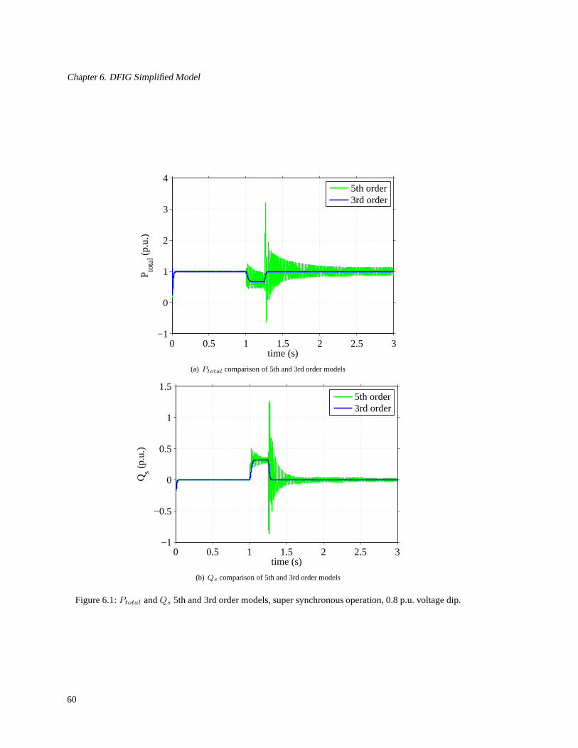
Chapter 6. DFIG Simplified Model
0 0.5 1 1.5 2 2.5 3−1
0
1
2
3
4
time (s)
P tota
l (p.
u.)
5th order3rd order
(a) Ptotal comparison of 5th and 3rd order models
0 0.5 1 1.5 2 2.5 3−1
−0.5
0
0.5
1
1.5
time (s)
Qs (
p.u.
)
5th order3rd order
(b) Qs comparison of 5th and 3rd order models
Figure 6.1:Ptotal andQs 5th and 3rd order models, super synchronous operation, 0.8 p.u. voltage dip.
60

6.3. Comparison of 5th order machine model to 3rd order machine model
0 0.5 1 1.5 2 2.5 3−4
−2
0
2
4
6
time (s)
P tota
l (p.
u.)
5th order3rd order
(a) Ptotal comparison of 5th and 3rd order models
0 0.5 1 1.5 2 2.5 3−6
−4
−2
0
2
time (s)
Qs (
p.u.
)
5th order3rd order
(b) Qs comparison of 5th and 3rd order models
Figure 6.2:Ptotal andQs 5th and 3rd order models, super synchronous operation, 0.25p.u. voltage dip.
61
Chapter 6. DFIG Simplified Model
6.4 Comparison of 3rd order machine model to 2nd order machinemodel
The next simplification made to the machine model is to assumethe rotor speed is fixed,or dωr
dt= 0, resulting in a 2nd order machine model. This simplificationis based on the
assumption that the time period of interest during a voltagedip is fast compared to therotor speed dynamics. In other words, it is assumed that the voltage dip occurs, and is sub-sequently removed from the system, in a short enough period of time that will not causea substantial change in rotor speed. In the interest of this thesis, it is not the actual changein rotor speed that is of importance, but rather the effect ofthe rotor speed dynamics onthe overall active and reactive power output from the DFIG during the transient event.Figures 6.3 and 6.4 show theP andQ response during super synchronous operation, forboth a shallow and severe voltage dip. The results indicate no substantial change to thePandQ by assuming the rotor speed is fixed.
The Appendix contains figures for a broader range of operating points, voltage dips,and other variables of interest, including the actual change in ωr. The results show therotor speed continuing to increase after the fault is cleared from the system. In reality, thespeed would be controlled to its reference value by pitchingthe rotor blades and therebydecreasing the input mechanical power. The rotor speed would then decelerate back tothe reference speed. In order to simulate this, a slow outer loop speed controller can beimplemented in the model.
6.5 Development of the final simplified DFIG model
The final simplification made to the DFIG model is based on an understanding of the finalsimplified model intended for use in PSS/E. As previously mentioned, the time step istypically 10 ms. This small of a time step limits what the simplified model will be ableto capture and represent. If it is assumed that 10 measuring points are needed to properlycapture a sinusoidal curve, then a model with a 10 ms time stepwill be limited to capturingfrequencies greater than 10 Hz. Therefore, the 50 Hz oscillations previously illustrated inthe 5th order detailed DFIG model will not be captured by a model implemented in PSS/Eat 10 ms time steps.
Based on this, the final assumption is that the action of the current controller is veryfast relative to the simulation time step. This leads to the final simplification:
1. The rotor current is equal to the rotor current reference value, and therefore thecurrent controller is omitted from the model.
The following is a summary of simplifications made to the basedetailed DFIG model:
62
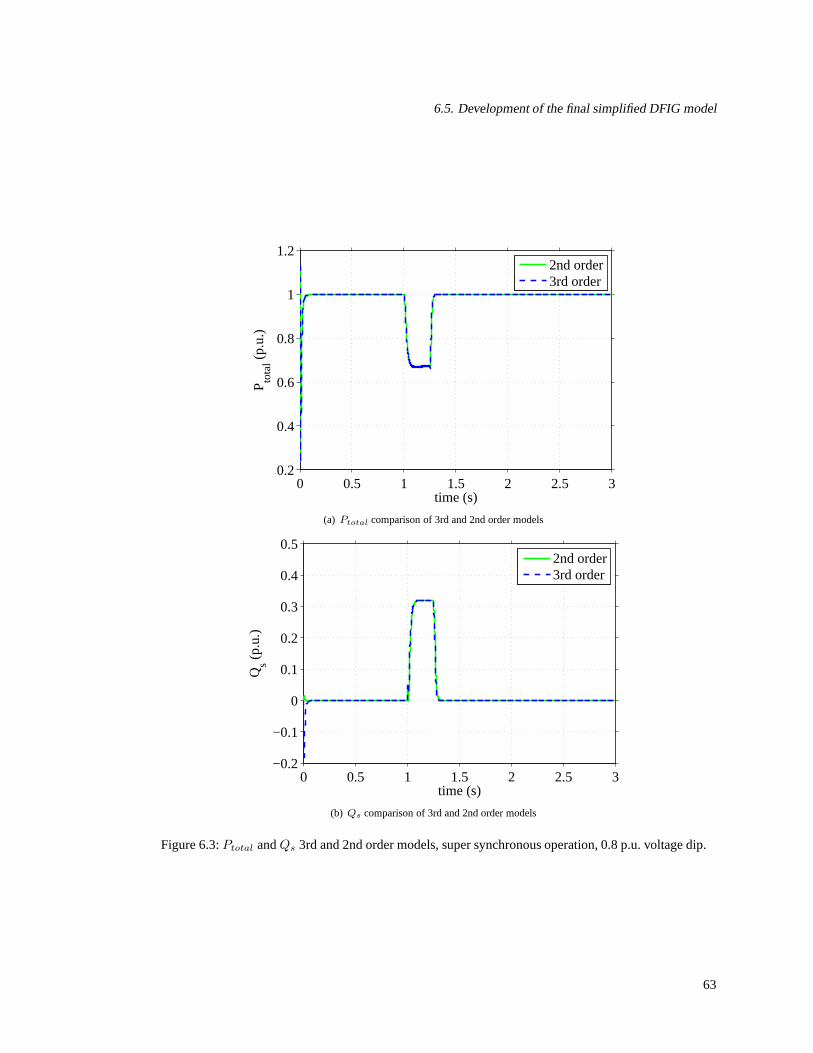
6.5. Development of the final simplified DFIG model
0 0.5 1 1.5 2 2.5 30.2
0.4
0.6
0.8
1
1.2
time (s)
P tota
l (p.
u.)
2nd order3rd order
(a) Ptotal comparison of 3rd and 2nd order models
0 0.5 1 1.5 2 2.5 3−0.2
−0.1
0
0.1
0.2
0.3
0.4
0.5
time (s)
Qs (
p.u.
)
2nd order3rd order
(b) Qs comparison of 3rd and 2nd order models
Figure 6.3:Ptotal andQs 3rd and 2nd order models, super synchronous operation, 0.8 p.u. voltage dip.
63

Chapter 6. DFIG Simplified Model
0 0.5 1 1.5 2 2.5 30
0.2
0.4
0.6
0.8
1
1.2
1.4
time (s)
P tota
l (p.
u.)
2nd order3rd order
(a) Ptotal comparison of 3rd and 2nd order models
0 0.5 1 1.5 2 2.5 3−0.2
−0.1
0
0.1
0.2
0.3
0.4
0.5
time (s)
Qs (
p.u.
)
2nd order3rd order
(b) Qs comparison of 3rd and 2nd order models
Figure 6.4:Ptotal andQs 3rd and 2nd order models, super synchronous operation, 0.25p.u. voltage dip.
64

6.5. Development of the final simplified DFIG model
1. The rotor and stator transients are neglected. ThereforedΨr
dtand dΨs
dt= 0.
2. The rotor speed is considered to be constant, as the time period of interest duringvoltage dips and stability analysis is fast relative to the rotor speed dynamics.
3. The mechanical torqueTm is considered constant over the time period of interest.Similar to the previous simplification, the dynamics of the wind speed and thus inputmechanical torque is slow compared to the electrical dynamics of the machine.
4. The current controller has been omitted, as the action of the current controller isconsidered to be instantaneous.
With these simplifications, equation (3.1) can be simplifiedto the following:
ur = Rrir + j(ωs − ωr)Ψr (6.1)
and inserting equation (3.4) into (6.1), yields
ur = Rrir + j(ωs − ωr)(Lmis + Lrir)
= Rrir + j(ωs − ωr)Lmis + j(ωs − ωr)Lrir
= Rrir + jsXmis + jsXrir (6.2)
where
Xm = ωsLm
Xr = ωsLr
Xs = ωsLs
s = slip =ωs − ωr
ωs
Equation (3.1) can also be simplified, using (3.3), as follows:
us = Rsis + jωsΨs
= Rsis + jωs(Lsis + Lmir)
= is(Rs + jωsLs) + jωsLmir (6.3)
yielding an equation that can be used to solve foris as:
65

Chapter 6. DFIG Simplified Model
is =us − jωsLmirRs + jωsLs
=us − jXmirRs + jXs
(6.4)
The simplified model is therefore represented by the previously defined set of alge-braic equations, with an outer P controller and an outer Q controller designed to providereactive power support per the E.ON grid code. Figure 6.5 represents a simplified controldiagram of the original 5th order machine model with currentcontroller and outer P and Qcontrollers, followed by the simplifications made in arriving at the final simplified modelcontrol diagram.
gridS
Rotor Back EMF
feedforward
Rotor current
controller
P & Q
controllers
Load
feedforward
Rdqi
Rdqi
*
Rdqi *
Rdqu
QP,
**,QP RSC RdquMachine
(a) Original control diagram of 5th order machine model withcurrent controller and outer P and Q controllers
gridS
Rotor Back EMF
feedforward
Rotor current
controller
P & Q
controllers
Load
feedforward
Rdqi
Rdqi
*
Rdqi *
Rdqu
QP,
**,QP RSC RdquMachine
(b) Simplifications made for final simplified model
gridS
P & Q
controllers
Load
feedforward
Rdqi
QP,
**,QP Algebraic
equations
(c) Final simplified model
Figure 6.5: Original detailed model control diagram and final simplified model
6.6 Comparison of 2nd order machine model to machine modeledasa set of algebraic equations
The final simplified model as described in the previous section is compared to the 2ndorder machine model. For this discussion, the final simplified model will be referred to
66

6.6. Comparison of 2nd order machine model to machine modeled as a set of algebraic equations
as just the ’simplified’ model. Figures 6.6 and 6.7 illustrate the two models for supersynchronous operation, with voltage dips of 0.8 p.u. and 0.25 p.u., respectively.Ptotal andQs are the only variables shown, with further documentation found in the Appendix.
The results of the comparison show good agreement between the two models. As ex-pected, the simplified model is not able to identify the transients that occur at the begin-ning and end of the voltage dip. The reactive power and activepower show near perfectagreement. This results in the conclusion that the simplified model is able to accuratelydemonstrate the trend of the active and reactive power as compared to the detailed 5thorder model.
67

Chapter 6. DFIG Simplified Model
0 0.5 1 1.5 2 2.5 3−0.2
0
0.2
0.4
0.6
0.8
1
1.2
time (s)
P tota
l (p.
u.)
2nd orderSimplified
(a) Ptotal comparison of 2nd order and simplified models
0 0.5 1 1.5 2 2.5 3−0.1
0
0.1
0.2
0.3
0.4
time (s)
Qs (
p.u.
)
2nd orderSimplified
(b) Qs comparison of 2nd order and simplified models
Figure 6.6:Ptotal andQs 2nd order and simplified models, super synchronous operation, 0.8 p.u. voltagedip.
68

6.6. Comparison of 2nd order machine model to machine modeled as a set of algebraic equations
0 0.5 1 1.5 2 2.5 3−0.2
0
0.2
0.4
0.6
0.8
1
1.2
time (s)
P tota
l (p.
u.)
2nd orderSimplified
(a) Ptotal comparison of 2nd order and simplified models
0 0.5 1 1.5 2 2.5 3−0.1
0
0.1
0.2
0.3
0.4
0.5
0.6
time (s)
Qs (
p.u.
)
2nd orderSimplified
(b) Qs comparison of 2nd order and simplified models
Figure 6.7:Ptotal andQs 2nd order and simplified models, super synchronous operation, 0.25 p.u. voltagedip.
69

Chapter 6. DFIG Simplified Model
70
Chapter 7
Conclusions and Future Work
7.1 Conclusions
The aim of this work was to develop a simplified model for the DFIG wind turbine forpower system stability studies with an emphasis on short-term voltage stability analyses.A detailed model of the DFIG was developed, and was compared to field measurements.Several simplifications to the detailed model were investigated and compared with thedetailed model.
Investigation of DC-chopper
The DC-chopper operation was analyzed. A simplified representation of the DC-chopperwas implemented in the detailed DFIG model. The DC-chopper is modeled by switchingthe converter operation to a diode rectifier when|ir| > ir,max. In this operation, the rotorvoltageur magnitude is determined by the DC-link voltage, and is in phase with the rotorcurrent. The results demonstrate the general response of the DFIG during diode rectifieroperation to be similar to the response without the diode rectifier. For this reason, theDC-chopper operation is not included in the subsequent simplified models.
Comparison to field measurements
The DFIG 5th order machine model with P and Q controllers is compared to a field mea-sured response of a DFIG to a severe voltage dip. The model is found to have reasonableagreement with the general response, however there are significant differences that requirefurther investigation.
71
Chapter 7. Conclusions and Future Work
Analysis of poorly damped poles of DFIG
The DFIG with current controller configuration is recognized as having poorly dampedpoles near line frequency (50 Hz). The poles are identified asbeing associated with the sta-tor flux. The poles are dependent in large part on the bandwidth of the current controllerand the stator resistance. Damping is improved by decreasing αcc or by increasingRs.Further damping efforts are investigated by implementing astator flux damping term thatis discussed in [5], which implements a feedback of the derivative of the flux. The methodsuccessfully damps the stator flux oscillations and active power oscillations, however itintroduces a few adverse effects including harmonics and higher reactive power oscilla-tions. In [5], it is noted that this method has a high sensitivity to voltage sags. Furtheranalysis of the flux damping methods is left for future work.
Development of simplified models
Simplified models were developed in discrete steps, starting with the 5th order detailedmodel. The simplifications and conclusions are as follows:
• Stator flux dynamics are neglected, ordΨs
dt= 0, resulting in a 3rd order machine
model. The stator flux oscillations are removed, resulting in a more general response.A comparison to the 5th order model shows the 3rd order model to follow the average5th order response. The simplification loses some information regarding the hightransient oscillations at the beginning of the voltage dip and at fault clearing.
• Rotor speed is fixed, ordωr
dt= 0, resulting in a 2nd order machine model. The 2nd
order model is compared to the 3rd order model. Although there is a change inωr
in the 3rd order model, there is not a significant impact to theP andQ response ascompared to the 2nd order model.
• The action of the current controller is considered to be instantaneous, and thereforethe current controller is omitted from the model. This results in the machine modelbeing omitted as well, and instead representing the machinevariables by a set ofalgebraic equations. The final simplified model is thereforea 0 order machine modelwith P andQ controllers, see Figure 7.1. The final simplified model is comparedto the 2nd order model with near perfect agreement. It is concluded that the finalsimplified model is an accurate representation of the general P andQ response ofthe DFIG.
72
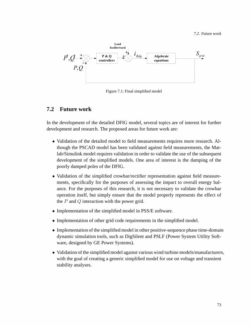
7.2. Future work
gridS
P & Q
controllers
Load
feedforward
Rdqi
QP,
**,QP Algebraic
equations
Figure 7.1: Final simplified model
7.2 Future work
In the development of the detailed DFIG model, several topics are of interest for furtherdevelopment and research. The proposed areas for future work are:
• Validation of the detailed model to field measurements requires more research. Al-though the PSCAD model has been validated against field measurements, the Mat-lab/Simulink model requires validation in order to validate the use of the subsequentdevelopment of the simplified models. One area of interest isthe damping of thepoorly damped poles of the DFIG.
• Validation of the simplified crowbar/rectifier representation against field measure-ments, specifically for the purposes of assessing the impactto overall energy bal-ance. For the purposes of this research, it is not necessary to validate the crowbaroperation itself, but simply ensure that the model properlyrepresents the effect oftheP andQ interaction with the power grid.
• Implementation of the simplified model in PSS/E software.
• Implementation of other grid code requirements in the simplified model.
• Implementation of the simplified model in other positive-sequence phase time-domaindynamic simulation tools, such as DigSilent and PSLF (PowerSystem Utility Soft-ware, designed by GE Power Systems).
• Validation of the simplified model against various wind turbine models/manufacturers,with the goal of creating a generic simplified model for use onvoltage and transientstability analyses.
73

Chapter 7. Conclusions and Future Work
74

References
[1] M. Bongiorno and T. Thiringer, “A generic DFIG model for voltage dip ride-throughanalysis,”IEEE Transactions on Energy Conversion, Submitted March 2012.
[2] “World market for wind turbines recovers and sets a new record: 42 GW of newcapacity in 2011, worldwide total capacity at 239 GW.” Feb 07, 2012. Accessiblefrom: http://www.windea.org, accessed May 01, 2012.
[3] “Renewables 2011 Global Status Report.” Published by Renewable Energy PolicyNetwork for the 21st Century, 2011. Accessible from: www.ren21.net.
[4] M. A. Bahmani, “Core loss calculation in amorphous high frequency high powertransformers with different topologies,” Master’s thesis, CHALMERS UNIVER-SITY OF TECHNOLOGY, 2011.
[5] A. Petersson,Analysis, Modeling, and Control of Doubly-Fed Induction Generatorsfor Wind Turbines. PhD thesis, Department of Energy and Environment ChalmersUniversity of Technology, 2003.
[6] A. Perdana,Dynamic Models of Wind Turbines, A contribution towards theEstab-lishment of Standardized Models of Wind Turbines for Power System Stability Stud-ies. PhD thesis, Department of Energy and Environment ChalmersUniversity ofTechnology, 2008.
[7] J. Fletcher and J. Yang,Introduction to the Doubly-Fed Induction Gener-ator For Wind Power Applications, Paths to Sustainable Energy, Dr ArtieNg (Ed.). InTech, available at: http://www.intechopen.com/books/paths-to-sustainable-energy/introduction-to-the-doubly-fed-induction-generator-for-wind-power-applications, 2010.
[8] T. Thiringer, J. Paixao, and M. Bongiorno, “Monitoring of the ride-through abilityof a 2mw wind turbine in tvaaker, halland,” tech. rep., Elforsk rapport 09:26, Stock-holm, Sweden, 2009.
[9] N. Mohan, T. Undeland, and W. Robbins,Power electronics converters, applica-tions, and design. Wiley, 2 edition, 1995.
75

References
[10] C.R.Kebler,Aktive dampfung der doppelt-gespeisten Drehstrommaschine. PhD the-sis, Technishen Universitat Carolo-Wilhelmina, 2000(inGerman).
[11] N. Ullah and T. Thiringer, “Variable speed wind turbines for power system stabil-ity enhancement,”IEEE Transactions on Energy Conversion, Vol.22, No.1, March2007.
[12] I. Erlich, J. Kretschmann, J. Fortmann, S. Mueller-Engelhardt, and H. Wrede, “Mod-eling of wind turbines based on doubly-fed induction generators for power systemstability studies,” Vol.22, No.3, August 2007.
[13] P. Ledesma and J. Usaola, “Doubly fed induction generator model for transient sta-bility analysis,”IEEE Transactions on Energy Conversion, Vol.20, No.2, June 2005.
[14] Y. Lei, A. Mullane, G. Lightbody, and R. Yacamini, “Modeling of the wind turbinewith a doubly fed induction generator for grid integration studies,” IEEE Transac-tions on Energy Conversion, Vol.21, No.1, March 2006.
[15] K. Clark, N. Miller, W. Price, and J. Sanchez-Gasca, “Modeling of GE wind turbine-generators for grid studies,” tech. rep., General ElectricInternational, Inc., Jan. 2008.
[16] N. Miller, J. Sanchez-Gasca, W. Price, and R. Delmerico, “Dynamic modeling ofGE 1.5 and 3.6 MW wind turbine-generators for stability simulations,”Proceedingof Power Engineering Society General Meeting, vol.3, July 2003, pp. 1977 - 1983.
76

Appendix A
Results from comparison of modelsimplifications
The appendix contains results from the comparison of various model simplifications. Itincludes results from various operating points, voltage dips, or machine variables notshown in the main document. Each section is dedicated to a separate model comparison.
77
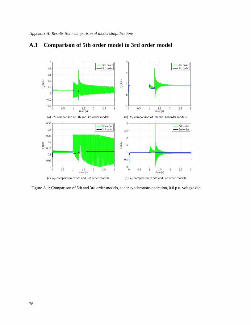
Appendix A. Results from comparison of model simplifications
A.1 Comparison of 5th order model to 3rd order model
0 0.5 1 1.5 2 2.5 3−0.4
−0.2
0
0.2
0.4
0.6
0.8
1
time (s)
P r (p.
u.)
5th order3rd order
(a) Pr comparison of 5th and 3rd order models
0 0.5 1 1.5 2 2.5 3−1
0
1
2
3
time (s)
P s (p.
u.)
5th order3rd order
(b) Ps comparison of 5th and 3rd order models
0 0.5 1 1.5 2 2.5 30
0.05
0.1
0.15
0.2
0.25
0.3
0.35
time (s)
u r (p.
u.)
5th order3rd order
(c) ur comparison of 5th and 3rd order models
0 0.5 1 1.5 2 2.5 30
0.5
1
1.5
2
2.5
3
time (s)
i r (p.
u.)
5th order3rd order
(d) ir comparison of 5th and 3rd order models
Figure A.1: Comparison of 5th and 3rd order models, super synchronous operation, 0.8 p.u. voltage dip.
78
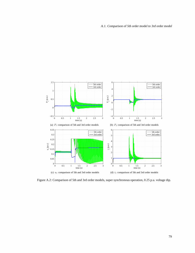
A.1. Comparison of 5th order model to 3rd order model
0 0.5 1 1.5 2 2.5 3−0.5
0
0.5
1
1.5
time (s)
P r (p.
u.)
5th order3rd order
(a) Pr comparison of 5th and 3rd order models
0 0.5 1 1.5 2 2.5 3−4
−2
0
2
4
6
time (s)
P s (p.
u.)
5th order3rd order
(b) Ps comparison of 5th and 3rd order models
0 0.5 1 1.5 2 2.5 30
0.05
0.1
0.15
0.2
0.25
0.3
0.35
time (s)
u r (p.
u.)
5th order3rd order
(c) ur comparison of 5th and 3rd order models
0 0.5 1 1.5 2 2.5 30
1
2
3
4
5
6
time (s)
i r (p.
u.)
5th order3rd order
(d) ir comparison of 5th and 3rd order models
Figure A.2: Comparison of 5th and 3rd order models, super synchronous operation, 0.25 p.u. voltage dip.
79

Appendix A. Results from comparison of model simplifications
0 0.5 1 1.5 2 2.5 3−3
−2
−1
0
1
2
3
4
time (s)
P tota
l (p.
u.)
5th order3rd order
(a) Ptotal comparison of 5th and 3rd order models
0 0.5 1 1.5 2 2.5 3−6
−4
−2
0
2
4
time (s)
Qs (
p.u.
)
5th order3rd order
(b) Qs comparison of 5th and 3rd order models
Figure A.3:Ptotal andQs 5th and 3rd order models, synchronous operation, 0.25 p.u. voltage dip.
80

A.1. Comparison of 5th order model to 3rd order model
0 0.5 1 1.5 2 2.5 3−0.5
0
0.5
1
1.5
time (s)
P r (p.
u.)
5th order3rd order
(a) Pr comparison of 5th and 3rd order models
0 0.5 1 1.5 2 2.5 3−4
−2
0
2
4
time (s)
P s (p.
u.)
5th order3rd order
(b) Ps comparison of 5th and 3rd order models
0 0.5 1 1.5 2 2.5 30
0.05
0.1
0.15
0.2
0.25
0.3
0.35
time (s)
u r (p.
u.)
5th order3rd order
(c) ur comparison of 5th and 3rd order models
0 0.5 1 1.5 2 2.5 30
1
2
3
4
5
time (s)
i r (p.
u.)
5th order3rd order
(d) ir comparison of 5th and 3rd order models
Figure A.4: Comparison of 5th and 3rd order models, synchronous operation, 0.25 p.u. voltage dip.
81
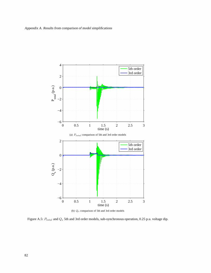
Appendix A. Results from comparison of model simplifications
0 0.5 1 1.5 2 2.5 3−6
−4
−2
0
2
4
time (s)
P tota
l (p.
u.)
5th order3rd order
(a) Ptotal comparison of 5th and 3rd order models
0 0.5 1 1.5 2 2.5 3−6
−4
−2
0
2
time (s)
Qs (
p.u.
)
5th order3rd order
(b) Qs comparison of 5th and 3rd order models
Figure A.5:Ptotal andQs 5th and 3rd order models, sub-synchronous operation, 0.25 p.u. voltage dip.
82
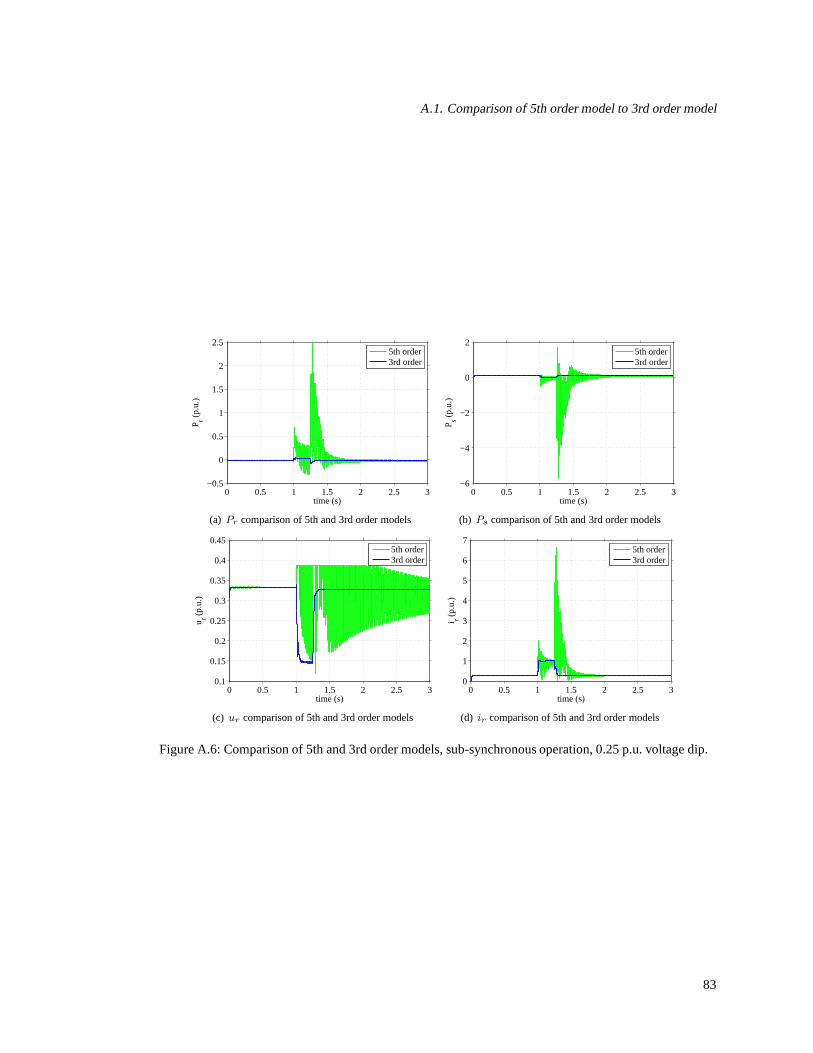
A.1. Comparison of 5th order model to 3rd order model
0 0.5 1 1.5 2 2.5 3−0.5
0
0.5
1
1.5
2
2.5
time (s)
P r (p.
u.)
5th order3rd order
(a) Pr comparison of 5th and 3rd order models
0 0.5 1 1.5 2 2.5 3−6
−4
−2
0
2
time (s)
P s (p.
u.)
5th order3rd order
(b) Ps comparison of 5th and 3rd order models
0 0.5 1 1.5 2 2.5 30.1
0.15
0.2
0.25
0.3
0.35
0.4
0.45
time (s)
u r (p.
u.)
5th order3rd order
(c) ur comparison of 5th and 3rd order models
0 0.5 1 1.5 2 2.5 30
1
2
3
4
5
6
7
time (s)
i r (p.
u.)
5th order3rd order
(d) ir comparison of 5th and 3rd order models
Figure A.6: Comparison of 5th and 3rd order models, sub-synchronous operation, 0.25 p.u. voltage dip.
83

Appendix A. Results from comparison of model simplifications
A.2 Comparison of 3rd order model to 2nd order model
0 0.5 1 1.5 2 2.5 30
0.05
0.1
0.15
0.2
0.25
time (s)
P r (p.
u.)
2nd order3rd order
(a) Pr comparison of 3rd and 2nd order models
0 0.5 1 1.5 2 2.5 30.2
0.4
0.6
0.8
1
time (s)
P s (p.
u.)
2nd order3rd order
(b) Ps comparison of 3rd and 2nd order models
0 0.5 1 1.5 2 2.5 30.05
0.1
0.15
0.2
0.25
0.3
time (s)
|ur| (
p.u.
)
2nd order3rd order
(c) ur comparison of 3rd and 2nd order models
0 0.5 1 1.5 2 2.5 30.2
0.4
0.6
0.8
1
1.2
time (s)
|i r| (p.
u.)
2nd order3rd order
(d) ir comparison of 3rd and 2nd order models
0 0.5 1 1.5 2 2.5 31.12
1.121
1.122
1.123
1.124
1.125
1.126
1.127
time (s)
wr (
p.u.
)
2nd order3rd order
(e) wr comparison of 3rd and 2nd order models
Figure A.7: Comparison of 3rd and 2nd order models, super synchronous operation, 0.8 p.u. voltage dip.
84

A.2. Comparison of 3rd order model to 2nd order model
0 0.5 1 1.5 2 2.5 3−0.1
−0.05
0
0.05
0.1
0.15
0.2
0.25
time (s)
P r (p.
u.)
2nd order3rd order
(a) Pr comparison of 3rd and 2nd order models
0 0.5 1 1.5 2 2.5 30
0.2
0.4
0.6
0.8
1
time (s)
P s (p.
u.)
2nd order3rd order
(b) Ps comparison of 3rd and 2nd order models
0 0.5 1 1.5 2 2.5 30
0.05
0.1
0.15
0.2
0.25
0.3
0.35
time (s)
|ur| (
p.u.
)
2nd order3rd order
(c) ur comparison of 3rd and 2nd order models
0 0.5 1 1.5 2 2.5 30.2
0.4
0.6
0.8
1
1.2
time (s)
|i r| (p.
u.)
2nd order3rd order
(d) ir comparison of 3rd and 2nd order models
0 0.5 1 1.5 2 2.5 3
1.13
1.14
1.15
1.16
1.17
1.18
time (s)
wr (
p.u.
)
2nd order3rd order
(e) wr comparison of 3rd and 2nd order models
Figure A.8: Comparison of 3rd and 2nd order models, super synchronous operation, 0.25 p.u. voltage dip.
85
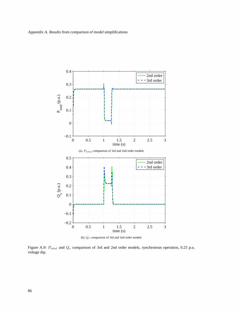
Appendix A. Results from comparison of model simplifications
0 0.5 1 1.5 2 2.5 3−0.1
0
0.1
0.2
0.3
0.4
time (s)
P tota
l (p.
u.)
2nd order3rd order
(a) Ptotal comparison of 3rd and 2nd order models
0 0.5 1 1.5 2 2.5 3−0.2
−0.1
0
0.1
0.2
0.3
0.4
0.5
time (s)
Qs (
p.u.
)
2nd order3rd order
(b) Qs comparison of 3rd and 2nd order models
Figure A.9:Ptotal andQs comparison of 3rd and 2nd order models, synchronous operation, 0.25 p.u.voltage dip.
86

A.2. Comparison of 3rd order model to 2nd order model
0 0.5 1 1.5 2 2.5 3−0.1
−0.05
0
0.05
0.1
time (s)
P r (p.
u.)
2nd order3rd order
(a) Pr comparison of 3rd and 2nd order models
0 0.5 1 1.5 2 2.5 30
0.05
0.1
0.15
0.2
0.25
0.3
0.35
time (s)
P s (p.
u.)
2nd order3rd order
(b) Ps comparison of 3rd and 2nd order models
0 0.5 1 1.5 2 2.5 30
0.05
0.1
0.15
0.2
0.25
time (s)
|ur| (
p.u.
)
2nd order3rd order
(c) ur comparison of 3rd and 2nd order models
0 0.5 1 1.5 2 2.5 30
0.2
0.4
0.6
0.8
1
1.2
1.4
time (s)
|i r| (p.
u.)
2nd order3rd order
(d) ir comparison of 3rd and 2nd order models
0 0.5 1 1.5 2 2.5 30.995
1
1.005
1.01
1.015
time (s)
wr (
p.u.
)
2nd order3rd order
(e) wr comparison of 3rd and 2nd order models
Figure A.10: Comparison of 3rd and 2nd order models, synchronous operation, 0.25 p.u. voltage dip.
87

Appendix A. Results from comparison of model simplifications
0 0.5 1 1.5 2 2.5 3−0.05
0
0.05
0.1
0.15
time (s)
P tota
l (p.
u.)
2nd order3rd order
(a) Ptotal comparison of 3rd and 2nd order models
0 0.5 1 1.5 2 2.5 3−0.4
−0.2
0
0.2
0.4
0.6
time (s)
Qs (
p.u.
)
2nd order3rd order
(b) Qs comparison of 3rd and 2nd order models
Figure A.11:Ptotal andQs comparison of 3rd and 2nd order models, sub-synchronous operation, 0.25 p.u.voltage dip.
88

A.2. Comparison of 3rd order model to 2nd order model
0 0.5 1 1.5 2 2.5 3−0.1
−0.05
0
0.05
0.1
time (s)
P r (p.
u.)
2nd order3rd order
(a) Pr comparison of 3rd and 2nd order models
0 0.5 1 1.5 2 2.5 3−0.05
0
0.05
0.1
0.15
time (s)
P s (p.
u.)
2nd order3rd order
(b) Ps comparison of 3rd and 2nd order models
0 0.5 1 1.5 2 2.5 30.1
0.15
0.2
0.25
0.3
0.35
time (s)
|ur| (
p.u.
)
2nd order3rd order
(c) ur comparison of 3rd and 2nd order models
0 0.5 1 1.5 2 2.5 30
0.2
0.4
0.6
0.8
1
1.2
1.4
time (s)
|i r| (p.
u.)
2nd order3rd order
(d) ir comparison of 3rd and 2nd order models
Figure A.12: Comparison of 3rd and 2nd order models, sub-synchronous operation, 0.25 p.u. voltage dip.
89

Appendix A. Results from comparison of model simplifications
A.3 Comparison of 2nd order model to simplified model
90

A.3. Comparison of 2nd order model to simplified model
0 0.5 1 1.5 2 2.5 30.8
0.85
0.9
0.95
1
time (s)
u sq (
p.u.
)
Simplified2nd order
(a) us comparison of 2nd order and simplified models
0 0.5 1 1.5 2 2.5 3−0.2
0
0.2
0.4
0.6
0.8
time (s)
P r (p.
u.)
2nd orderSimplified
(b) Pr comparison of 2nd order and simplified models
0 0.5 1 1.5 2 2.5 3−0.2
0
0.2
0.4
0.6
0.8
1
1.2
time (s)
P s (p.
u.)
2nd orderSimplified
(c) Ps comparison of 2nd order and simplified models
0 0.5 1 1.5 2 2.5 30.2
0.4
0.6
0.8
1
1.2
time (s)
|i r| (p.
u.)
2nd orderSimplified
(d) ir comparison of 2nd order and simplified models
0 0.5 1 1.5 2 2.5 30
0.2
0.4
0.6
0.8
time (s)
|ur| (
p.u.
)
2nd orderSimplified
(e) ur comparison of 2nd order and simplified models
Figure A.13: Comparison of 2nd order and simplified models, super synchronous operation, 0.8 p.u. voltagedip.
91

Appendix A. Results from comparison of model simplifications
0 0.5 1 1.5 2 2.5 30.2
0.4
0.6
0.8
1
1.2
time (s)
u sq (
p.u.
)
Simplified2nd order
(a) us comparison of 2nd order and simplified models
0 0.5 1 1.5 2 2.5 3−0.2
0
0.2
0.4
0.6
0.8
time (s)P r (
p.u.
)
2nd orderSimplified
(b) Pr comparison of 2nd order and simplified models
0 0.5 1 1.5 2 2.5 3−0.2
0
0.2
0.4
0.6
0.8
1
1.2
time (s)
P s (p.
u.)
2nd orderSimplified
(c) Ps comparison of 2nd order and simplified models
0 0.5 1 1.5 2 2.5 30.2
0.4
0.6
0.8
1
1.2
time (s)
|i r| (p.
u.)
2nd orderSimplified
(d) ir comparison of 2nd order and simplified models
0 0.5 1 1.5 2 2.5 30
0.2
0.4
0.6
0.8
time (s)
|ur| (
p.u.
)
2nd orderSimplified
(e) ur comparison of 2nd order and simplified models
Figure A.14: Comparison of 2nd order and simplified models, super synchronous operation, 0.25 p.u. volt-age dip.
92

A.3. Comparison of 2nd order model to simplified model
0 0.5 1 1.5 2 2.5 3−0.1
0
0.1
0.2
0.3
0.4
time (s)
P tota
l (p.
u.)
2nd orderSimplified
(a) Ptotal comparison of 2nd order and simplified models
0 0.5 1 1.5 2 2.5 3−0.1
0
0.1
0.2
0.3
0.4
0.5
0.6
time (s)
Qs (
p.u.
)
2nd orderSimplified
(b) Qs comparison of 2nd order and simplified models
Figure A.15:Ptotal andQs comparison of 2nd order and simplified models, synchronous operation, 0.25p.u. voltage dip.
93
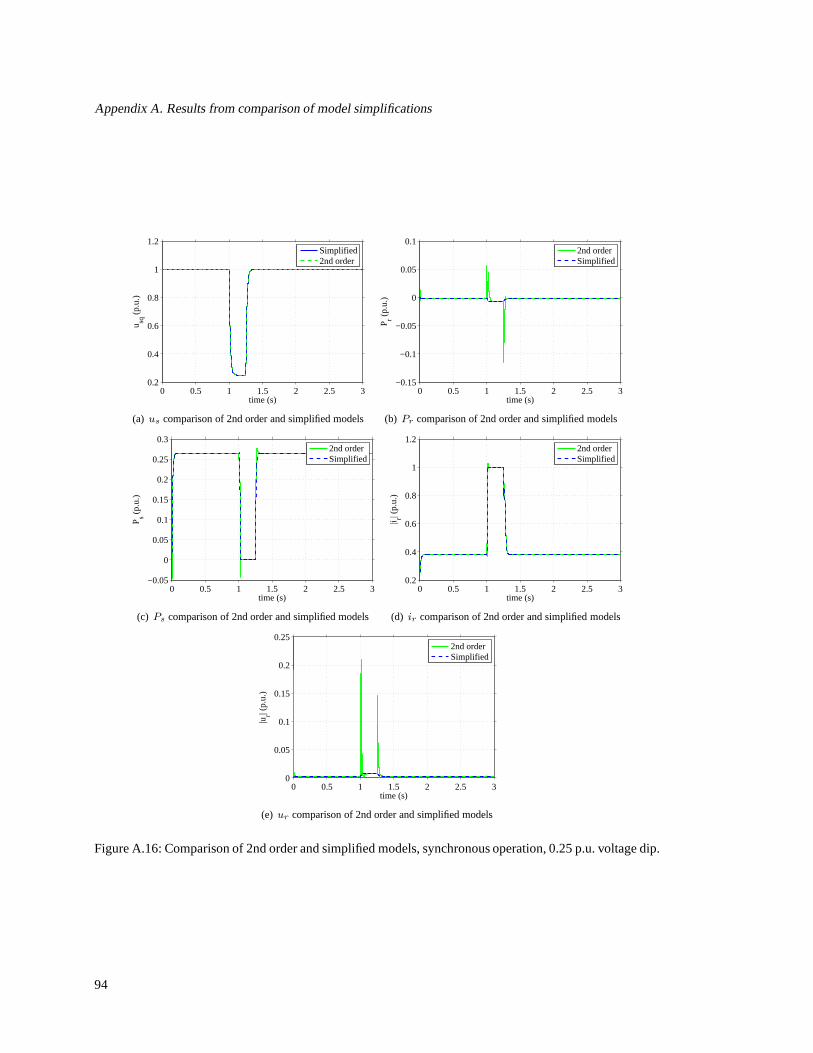
Appendix A. Results from comparison of model simplifications
0 0.5 1 1.5 2 2.5 30.2
0.4
0.6
0.8
1
1.2
time (s)
u sq (
p.u.
)
Simplified2nd order
(a) us comparison of 2nd order and simplified models
0 0.5 1 1.5 2 2.5 3−0.15
−0.1
−0.05
0
0.05
0.1
time (s)
P r (p.
u.)
2nd orderSimplified
(b) Pr comparison of 2nd order and simplified models
0 0.5 1 1.5 2 2.5 3−0.05
0
0.05
0.1
0.15
0.2
0.25
0.3
time (s)
P s (p.
u.)
2nd orderSimplified
(c) Ps comparison of 2nd order and simplified models
0 0.5 1 1.5 2 2.5 30.2
0.4
0.6
0.8
1
1.2
time (s)
|i r| (p.
u.)
2nd orderSimplified
(d) ir comparison of 2nd order and simplified models
0 0.5 1 1.5 2 2.5 30
0.05
0.1
0.15
0.2
0.25
time (s)
|ur| (
p.u.
)
2nd orderSimplified
(e) ur comparison of 2nd order and simplified models
Figure A.16: Comparison of 2nd order and simplified models, synchronous operation, 0.25 p.u. voltage dip.
94
Related Documents