Deep Single Image Camera Calibration with Radial Distortion · 2020-02-25 · Deep Single Image Camera Calibration with Radial Distortion Manuel Lopez-Antequera´ * Roger Mar´ı

Deep Single Image Camera Calibration with Radial Distortion

Manuel Lopez-Antequera* Roger Marı † Pau Gargallo* Yubin Kuang*

Javier Gonzalez-Jimenez‡ Gloria Haro§

Abstract

Single image calibration is the problem of predictingthe camera parameters from one image. This problem isof importance when dealing with images collected in un-controlled conditions by non-calibrated cameras, such ascrowd-sourced applications. In this work we propose amethod to predict extrinsic (tilt and roll) and intrinsic (fo-cal length and radial distortion) parameters from a singleimage. We propose a parameterization for radial distor-tion that is better suited for learning than directly predict-ing the distortion parameters. Moreover, predicting addi-tional heterogeneous variables exacerbates the problem ofloss balancing. We propose a new loss function based onpoint projections to avoid having to balance heterogeneousloss terms. Our method is, to our knowledge, the first tojointly estimate the tilt, roll, focal length, and radial distor-tion parameters from a single image. We thoroughly analyzethe performance of the proposed method and the impact ofthe improvements and compare with previous approachesfor single image radial distortion correction.

1. Introduction

Single image calibration deals with the prediction ofcamera parameters from a single image. Camera calibrationis the first step in many computer vision tasks e.g. Structurefrom Motion, especially in applications where the captur-ing conditions are not controlled is particularly challenging,such as those relying on crowdsourced imagery.

The process of image formation is well understood andhas been studied extensively in computer vision [1], allow-ing for very precise calibration of cameras when there areenough geometric constraints to fit the camera model. Thisis a well established practice that is performed daily on anindustrial scale, but requires a set of images taken for thepurpose of calibration. Geometric based methods can alsobe used with images taken outside of the lab, performing

*Mapillary, [email protected]†CMLA, ENS Cachan, [email protected]‡Universidad de Malaga, [email protected]§Universitat Pompeu Fabra, [email protected]

Figure 1. Our method is able to recover extrinsic (tilt, roll) andintrinsic (focal length and radial distortion) parameters from sin-gle images (top row). In the bottom row, we visualize the predictedparameters by undistorting the input images and overlaying a hori-zon line, which is a proxy for the tilt and roll angles.

best on images depicting man-made environments present-ing strong cues such as vanishing points and straight linesthat can be used to recover the camera parameters [2, 3].However, since geometric-based methods rely on detect-ing and processing specific cues such as straight lines andvanishing points, they lack robustness to images taken inunstructured environments, with low quality equipment ordifficult illumination conditions.

In this work we present a method to recover extrinsic(tilt, roll) and intrinsic (focal length and radial distortion)parameters given a single image. We train a convolutionalneural network to perform regression on alternative repre-sentations of these parameters which are better suited forprediction from a single image.

We advance with respect to the state of the art with threemain contributions: 1. a single parameter representation fork1 and k2 based on a large database of real calibrated cam-eras. 2. a representation of the radial distortion that is in-dependent from the focal length and more easily learned bythe network. 3. a new loss function based on the projec-tion of points to alleviate the problem of balancing hetero-

1

geneous loss components.To the best of our knowledge, this work is the first

to jointly estimate the camera orientation and calibrationjointly while including radial distortion.

2. Related WorkRecent works have leveraged the success of convolu-

tional neural networks and proposed using learned methodsto estimate camera parameters. Through training, a CNNcan learn to detect the subtle but relevant cues for the task,extending the range of scenarios where single image cali-bration is feasible.

Different components of the problem of learned singleimage calibration have been studied in the past: Workmanet al. [4] trained a CNN to perform regression of the fieldof view of a pinhole camera, later focusing on detecting thehorizon line on images [5], which is a proxy for the tilt androll angles of the camera if the focal length is known.

Rong et al. [6] use a classification approach to calibratethe single-parameter radial distortion model from Fitzgib-bon [7]. Hold-Geoffroy et al. [8] first combined extrin-sic and intrinsic calibration in a single network, predictingthe tilt, roll and focal length of a pinhole camera througha classification approach. They relied on upright 360 de-gree imagery to synthetically generate images of arbitrarysize, focal length and rotation, an approach that we borrowto generate training data. Classic and learned methods canbe combined. In [9], learned methods are used to obtain aprior distribution on the possible camera parameters, whichare then refined using classic methods, accelerating the ex-ecution time and robustness with respect to fully geomet-ric methods. We do not follow such an approach in thiswork. However, the prediction produced by our method canbe used as a prior in such pipelines.

When training a convolutional neural network for sin-gle image calibration, the loss function is an aggregate ofseveral loss components, one for each parameter. This sce-nario is usually known as multi-task learning [10]. Worksin multi-task learning deal with the challenges faced whentraining a network to perform several tasks with separatelosses. Most of these approaches rely on a weighted sumof the loss components, differing on the manner in whichthe weights are set at training time: Kendall et al. [11] useGaussian and softmax likelihoods (for regression and clas-sification, respectively) to weight the different loss compo-nents according to a task-dependent uncertainty. In con-trast to these uncertainty based methods, Chen et al. [12]determine the value of the weights by adjusting the gradientmagnitudes associated to each loss term.

When possible, domain knowledge can be used insteadof task-agnostic methods in order to balance loss compo-nents: Yin et al. [13] perform single image calibration of an8-parameter distortion model of fisheye lenses. They note

the difficulty of balancing loss components of different na-ture when attempting to directly minimize the parameter er-rors and propose an alternative based on the photometricerror. In this work, we also explore the problem of balanc-ing loss components for camera calibration and propose afaster approach based on projecting points using the cam-era model instead of deforming the image to calculate thephotometric error.

3. MethodWe briefly summarize our method and describe the de-

tails in subsequent sections.We train a convolutional neural network to predict the

extrinsic and intrinsic camera parameters of a given image.To achieve this, we use independent regressors that share acommon pretrained network architecture as the feature ex-tractor, which we fine-tune for the task. Instead of trainingthese regressors to predict the tilt θ, roll ψ, focal length f ,and distortion parameters k1 and k2, we use proxy variablesthat are directly visible in the image and independent fromeach other. To obtain training data for the network, we relyon a diverse panorama dataset from which we crop and dis-tort panoramas to synthesize images taken using perspectiveprojection cameras with arbitrary parameters.

3.1. Camera Model

We consider a camera model with square pixels and cen-tered principal point that is affected by radial distortion thatcan be modeled by a two-parameter polynomial distortion.

The projection model is the following. World pointsare transformed to local reference frame of the camera byapplying a rotation R and translation t. Let (X,Y, Z) bethe coordinates of a 3D point expressed in the local refer-ence frame of the camera. The point is projected to theplane Z = 1 to obtain the normalized image coordinates(x, y) = (X/Z, Y/Z). Radial distortion scales the normal-ized coordinates by a factor d, which is a function of theradius r and the distortion coefficients k1 and k2:

r =√x2 + y2

d = 1 + k1r2 + k2r

4 (1)(xd, yd) = (d x, d y). (2)

Finally, the focal length f scales the normalized and dis-torted image coordinates to pixels: (ud, vd) = (f xd, f yd).

In this work, we do not attempt to recover the positionof the images nor the full rotation matrix, as that would re-quire the network to memorize the appearance of the en-vironment, turning our problem of single image calibrationinto a different problem, so-called place recognition.

Instead, we rely on the horizon line as a reference frame,leaving two free parameters: the tilt θ and roll ψ anglesof the camera with respect to the horizon. This allows a

ρ

τ

h = 2f tan(Fv

2 )

h

ψ

CC BY 2.0, photo by m01229

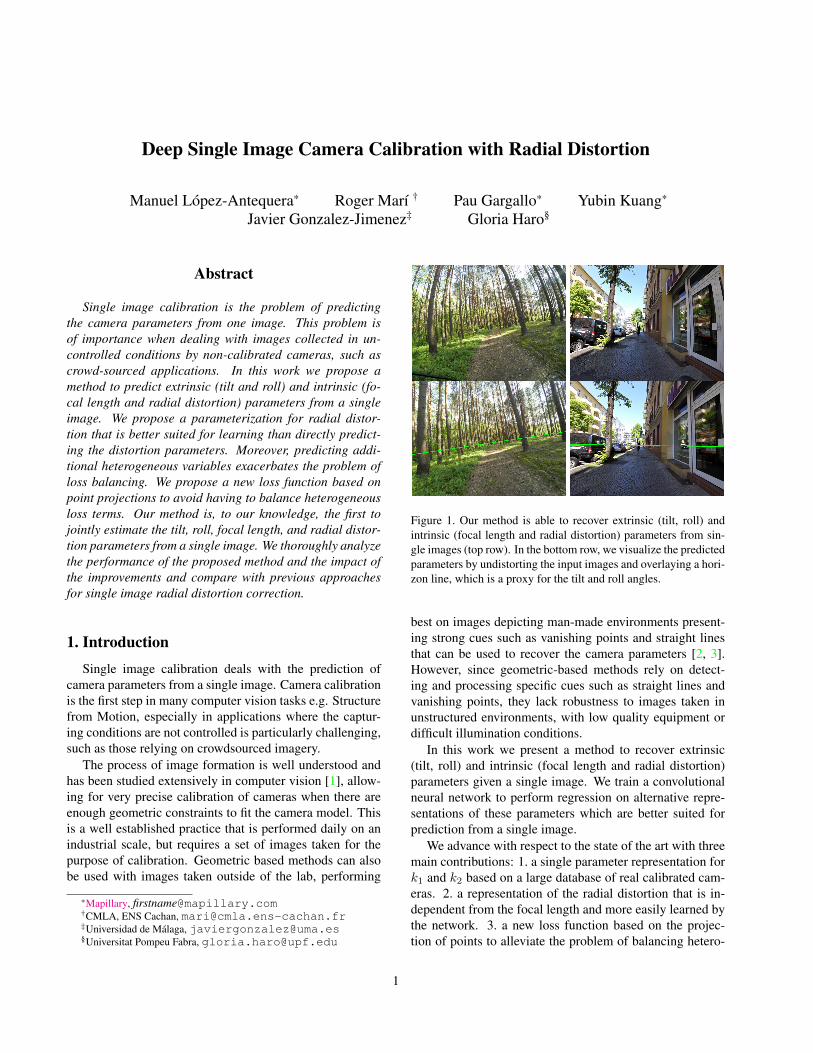
Figure 2. We use an alternative representation for the camera pa-rameters that is based on image cues: The network is trained topredict the distorted offset ρ and vertical field of view Fv insteadof the tilt θ and focal length f . The undistorted offset τ is wherethe horizon would be if there was no radial distortion.

network to be trained using images from a set of locations togeneralize well to other places, as long as there is sufficientvisual diversity.

Thus, the parameters to be recovered by the network arethe tilt and roll angles (θ, ψ), the focal length f and distor-tion parameters k1 and k2.

3.2. Parameterization

As revealed by previous work [4, 5, 8], an adequate pa-rameterization of the variables to predict can greatly bene-fit convergence and final performance of the network. Forthe case of camera calibration, parameters such as the fo-cal length or the tilt angles are difficult to interpret from theimage content. Instead, they can be better represented byproxy parameters that are directly observable in the image.We begin by following already existing parameterizationsand propose new ones required to deal with the case of ra-dially distorted images. We refer the reader to Figure 2 tocomplement the text in this section.

We start by defining the horizon line as done in [5]: “Theimage location of the horizon line is defined as the projec-tion of the line at infinity for any plane which is orthogonalto the local gravity vector.”. This definition also holds truefor cameras with radial distortion, however, the projectionof the horizon line in the image will not necessarily remaina straight line.1

The focal length f is related to the vertical and horizontalfields of view through the image size of height h and widthw. The field of view is directly related to the image contentand is thus more suitable for the task. We use the vertical

1If there is radial distortion, the horizon line (and any other straightlines) will only be projected as a straight line in the image if it passesthrough the center of the image.

−0.4 −0.3 −0.2 −0.1 0.0

k1

0.00

0.05

0.10

0.15

k2

0.019k1 + 0.805k21

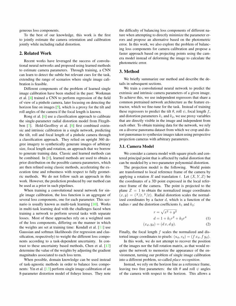
Figure 3. A distribution of k1 and k2 recovered from a large setof SfM reconstructions reveals that, for many real cameras, theseparameters lie close to a one-dimensional manifold. We rely onthis to simplify our camera model such that k2 is a function of k1.

field of view, defined as

Fv = 2arctanh

2f, (3)

as a proxy for the focal length. During deployment of thenetwork, the image height h is known and the focal lengthcan be recovered from the predicted Fv .

The roll angle ψ of the camera is directly represented inthe image as the angle of the horizon line, not requiring anyalternative parameterization.

A good proxy for the tilt angle θ is the distance ρ fromthe center of the image to the horizon line. Previous workused such a parameterization for pinhole cameras with nodistortion [5], however, the presence of radial distortioncomplicates this relationship slightly. We first define theundistorted offset τ as the distance from the image center tothe horizon line when there is no radial distortion. It can beexpressed as a function of the tilt angle and the focal length:

τ = f tan(θ). (4)

The distorted offset ρ is related with τ by the radial distor-tion scaling as expressed in Equation 2.

3.2.1 Distortion coefficients in real cameras

We simplify the radial distortion model by expressing k2 asa function of k1. This decision was initially motivated by apractical consideration: independently sampling k1 and k2often results in unrealistically distorted images. For imagesfrom real lenses, the distortion coefficients seem to lie in amanifold. We confirm this by studying the distribution ofk1 and k2 on a large collection of camera calibrations.

We use Structure from Motion (SfM) with self-calibration to perform reconstructions on image sequencestaken with real cameras to estimate their parameters. We

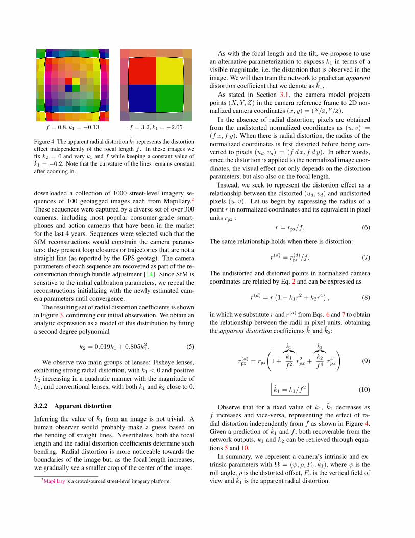
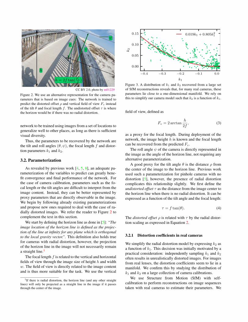
f = 0.8, k1 = −0.13 f = 3.2, k1 = −2.05

Figure 4. The apparent radial distortion k1 represents the distortioneffect independently of the focal length f . In these images wefix k2 = 0 and vary k1 and f while keeping a constant value ofk1 = −0.2. Note that the curvature of the lines remains constantafter zooming in.

downloaded a collection of 1000 street-level imagery se-quences of 100 geotagged images each from Mapillary.2

These sequences were captured by a diverse set of over 300cameras, including most popular consumer-grade smart-phones and action cameras that have been in the marketfor the last 4 years. Sequences were selected such that theSfM reconstructions would constrain the camera parame-ters: they present loop closures or trajectories that are not astraight line (as reported by the GPS geotag). The cameraparameters of each sequence are recovered as part of the re-construction through bundle adjustment [14]. Since SfM issensitive to the initial calibration parameters, we repeat thereconstructions initializing with the newly estimated cam-era parameters until convergence.

The resulting set of radial distortion coefficients is shownin Figure 3, confirming our initial observation. We obtain ananalytic expression as a model of this distribution by fittinga second degree polynomial

k2 = 0.019k1 + 0.805k21. (5)

We observe two main groups of lenses: Fisheye lenses,exhibiting strong radial distortion, with k1 < 0 and positivek2 increasing in a quadratic manner with the magnitude ofk1, and conventional lenses, with both k1 and k2 close to 0.

3.2.2 Apparent distortion

Inferring the value of k1 from an image is not trivial. Ahuman observer would probably make a guess based onthe bending of straight lines. Nevertheless, both the focallength and the radial distortion coefficients determine suchbending. Radial distortion is more noticeable towards theboundaries of the image but, as the focal length increases,we gradually see a smaller crop of the center of the image.

2Mapillary is a crowdsourced street-level imagery platform.

As with the focal length and the tilt, we propose to usean alternative parameterization to express k1 in terms of avisible magnitude, i.e. the distortion that is observed in theimage. We will then train the network to predict an apparentdistortion coefficient that we denote as k1.

As stated in Section 3.1, the camera model projectspoints (X,Y, Z) in the camera reference frame to 2D nor-malized camera coordinates (x, y) = (X/Z, Y/Z).

In the absence of radial distortion, pixels are obtainedfrom the undistorted normalized coordinates as (u, v) =(f x, f y). When there is radial distortion, the radius of thenormalized coordinates is first distorted before being con-verted to pixels (ud, vd) = (f d x, f d y). In other words,since the distortion is applied to the normalized image coor-dinates, the visual effect not only depends on the distortionparameters, but also also on the focal length.

Instead, we seek to represent the distortion effect as arelationship between the distorted (ud, vd) and undistortedpixels (u, v). Let us begin by expressing the radius of apoint r in normalized coordinates and its equivalent in pixelunits rpx :

r = rpx/f. (6)

The same relationship holds when there is distortion:

r(d) = r(d)px /f. (7)

The undistorted and distorted points in normalized cameracoordinates are related by Eq. 2 and can be expressed as

r(d) = r(1 + k1r

2 + k2r4), (8)

in which we substitute r and r(d) from Eqs. 6 and 7 to obtainthe relationship between the radii in pixel units, obtainingthe apparent distortion coefficients k1and k2:

r(d)px = rpx

(1 +

k1︷︸︸︷k1f2

r2px +

k2︷︸︸︷k2f4

r4px

)(9)

k1 = k1/f2 (10)

Observe that for a fixed value of k1, k1 decreases asf increases and vice-versa, representing the effect of ra-dial distortion independently from f as shown in Figure 4.Given a prediction of k1 and f , both recoverable from thenetwork outputs, k1 and k2 can be retrieved through equa-tions 5 and 10.

In summary, we represent a camera’s intrinsic and ex-trinsic parameters with Ω = (ψ, ρ, Fv, k1), where ψ is theroll angle, ρ is the distorted offset, Fv is the vertical field ofview and k1 is the apparent radial distortion.

xn

p1

pn

p′n

f ′

p′1

x1

f

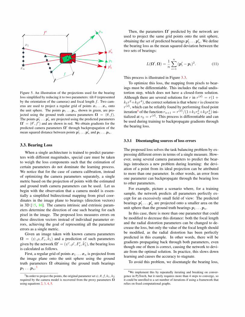
Figure 5. An illustration of the projections used for the bearingloss simplified by reducing it to two parameters: tilt θ (representedby the orientation of the cameras) and focal length f . Two cam-eras are used to project a regular grid of points x1 . . .xn ontothe unit sphere. The points p1 . . .pn, shown in green, are pro-jected using the ground truth camera parameters Ω = (θ, f).The points p′

1 . . .p′n are projected using the predicted parameters

Ω′ = (θ′, f ′) and are shown in red. We obtain gradients for thepredicted camera parameters Ω′ through backpropagation of themean squared distance between points p′

1 . . .p′n and p1 . . .pn.

3.3. Bearing Loss

When a single architecture is trained to predict parame-ters with different magnitudes, special care must be takento weigh the loss components such that the estimation ofcertain parameters do not dominate the learning process.We notice that for the case of camera calibration, insteadof optimizing the camera parameters separately, a singlemetric based on the projection of points with the estimatedand ground truth camera parameters can be used. Let usbegin with the observation that a camera model is essen-tially a simplified bidirectional mapping from pixel coor-dinates in the image plane to bearings (direction vectors)in 3D [15, 16]. The camera intrinsic and extrinsic param-eters determine the direction of one such bearing for eachpixel in the image. The proposed loss measures errors onthese direction vectors instead of individual parameter er-rors, achieving the goal of representing all the parametererrors as a single metric.

Given an image taken with known camera parametersΩ = (ψ, ρ, Fv, k1) and a prediction of such parametersgiven by the network Ω′ = (ψ′, ρ′, F ′v, k

′1), the bearing loss

is calculated as follows.First, a regular grid of points x1 . . .xn is projected from

the image plane onto the unit sphere using the groundtruth parameters Ω obtaining the ground truth bearingsp1 . . .pn.3

3In order to project the points, the original parameter set ψ, θ, f, k1, k2required by the camera model is recovered from the proxy parameters Ωusing equations 2, 3, 4, 5.

Then, the parameters Ω′ predicted by the network areused to project the same grid points onto the unit sphere,obtaining the set of predicted bearings p′1 . . .p

′n. We define

the bearing loss as the mean squared deviation between thetwo sets of bearings:

L(Ω′,Ω) =1

n

n∑i=1

(p′i − pi)2. (11)

This process is illustrated in Figure 3.3.To optimize this loss, the mapping from pixels to bear-

ings must be differentiable. This includes the radial undis-tortion step, which does not have a closed-form solution.Although there are several solutions for r in r(d) = r(1 +k1r

2+k2r4), the correct solution is that where r is closest to

r(d), which can be reliably found by performing fixed pointiteration4 of the function rn+1 = r(d)/(1+k1r

2n+k2r

4n) ini-

tialized at r0 = r(d). This process is differentiable and canbe used during training to backpropagate gradients throughthe bearing loss.

3.3.1 Disentangling sources of loss errors

The proposed loss solves the task balancing problem by ex-pressing different errors in terms of a single measure. How-ever, using several camera parameters to predict the bear-ings introduces a new problem during learning: the devi-ation of a point from its ideal projection can be attributedto more than one parameter. In other words, an error fromone parameter can backpropagate through the bearing lossto other parameters.

For example, picture a scenario where, for a trainingsample, the network predicts all parameters perfectly ex-cept for an excessively small field of view: The predictedbearings p′1 . . .p

′n are projected onto a smaller area on the

unit sphere than the ground truth bearings p1 . . .pn.In this case, there is more than one parameter that could

be modified to decrease this distance: both the focal lengthand the radial distortion parameters can be changed to de-crease the loss, but only the value of the focal length shouldbe modified, as the radial distortion has been perfectlypredicted in this example. In other words, there will begradients propagating back through both parameters, eventhough one of them is correct, causing the network to devi-ate from the optimal solution. In practice, this slows downlearning and causes the accuracy to stagnate.

To avoid this problem, we disentangle the bearing loss,

4We implement this by repeatedly iterating and breaking on conver-gence in PyTorch, but it rarely requires more than 4 steps to converge, soit could be unrolled to a set number of iterations if using a framework thatrelies on fixed computational graphs.

Parameter Distribution Values

Pan φ Uniform [0, 2π)Distorted offset ρ Normal µ = 0.046, σ = 0.6Roll ψ Cauchy x0 = 0, γ ∈ 0.001, 0.1Aspect ratio w/h Varying 1/1 9%, 5/4 1%, 4/3 66%,

3/2 20%, 16/9 4%Focal length f Uniform [13, 38]Distortion k1 Uniform [−0.4, 0]Distortion k2 k2 = 0.019k1 + 0.805k21

Table 1. Distribution of the camera parameters used to generate ourtraining and validation sets. Units: f - mm, ψ- radians, ρ- fractionof image height.

evaluating it individually for each parameter ψ, ρ, Fv , k1:

Lψ = L((ψGT , ρGT , FGTv , kGT1 ),Ω)

Lρ = L((ψGT , ρGT , FGTv , kGT1 ),Ω)

LFv= L((ψGT , ρGT , FGTv , kGT1 ),Ω)

Lk1 = L((ψGT , ρGT , FGTv , kGT1 ),Ω)

L∗ =Lψ + Lρ + LFv

+ Lk14

(12)

This modification of the loss function greatly increasesconvergence and final accuracy, while maintaining the mainadvantage of the bearing loss of expressing all parametererrors in the same units.

3.4. Dataset

We use the SUN360 panorama dataset [17] to artificiallygenerate images taken with by cameras with arbitrary panφ, tilt θ, roll ψ, focal length f and distortion k1. High reso-lution images of 9104 × 4452 pixels are used to render thetraining and evaluation images as follows:

First, we divide the SUN360 dataset into training, evalu-ation and test sets of 55681, 1298 and 165 images, respec-tively. Separating the panorama dataset before generatingthe perspective images ensures that no panoramas are usedto generate crops that end up in different datasets.

Then, from each panorama in the training and validationsets, we generate seven perspective images by randomlysampling the pan φ, offset ρ, roll ψ, aspect ratio, focallength f and the distortion coefficient k1 from the proba-bility distributions found in Table 1, resulting in a dataset of389, 767 training and 9, 086 validation images.

In a practical scenario, the distribution of the training setshould be designed to mimic that of the images that willbe used when deploying the network. For this paper wehave selected simple distributions that are consistent withthose found in large online image databases: we take thesame distributions as in previous work [8], except for theinclusion of k1 for radial distortion. Additionally, we have

modified the distribution of f to be uniform in order to avoidobtaining images with large focal lengths since the effect ofradial distortion in such images is negligible5.

For the test set we followed a different approach,sampling from the 165 panoramas in the panorama testset more extensively and evenly by taking 100 cropsfrom each panorama and using uniform distributionsalso for the roll angle ψ ∼ U(−π/2, π/2), distortedoffset ρ ∼ U(−1.2, 1.2) and aspect ratios w/h ∼U1/1, 5/4, 4/3, 3/2, 16/9. This results in 16, 500 im-ages for our test set.

4. ExperimentsWe use a densenet-161 [18] pretrained on ImageNet [19]

as a feature extractor and replace the classifier layer withfour regressors, each consisting of a ReLU-activated hiddenlayer of 256 units followed by the output unit.

As explained before, images are generated with a vari-ety of aspect ratios. We experimented with several waysof feeding such images to the network: resizing, center-cropping and letterboxing. Previous authors noticed bet-ter results by square-cropping the images [5]. Like Hold-Geoffroy et al. [8], we obtained best results by resizing theimages to a square. Even though there is deformation in theimage when its aspect ratio is changed, it appears to be thatkeeping all of the image content by not cropping the imageis preferable to any negative effect the warping itself mayproduce. All images are thus scaled to 224 × 224 pixelsbefore feeding them to the network.

We train the network by directly minimizing parametererrors as well as using the proposed bearing loss. In the firstcase, we minimize a sum of weighted Huber losses:

LH = wψLHψ + wρL

Hρ + wFvL

HFv

+ wk1LHk1

(13)

For the bearing loss, the predicted and ground truth parame-ters of each image are used to project bearings as describedin Section 3.3.

In both cases we minimize the losses using an Adam op-timizer with learning rate 10−4 in batches of 42 images.Through early stopping we finish training after 8-10 epochs.We use a step learning rate decay such that the learning rateis reduced by 30% at the end of each epoch.

4.1. Evaluation of the Loss Functions

We evaluate the bearing loss from Section 3.3 and com-pare it to the weighted Huber loss (Eq. 13). The Huber losswith unit weights performs better.

The results are comparable, except for the prediction ofk1 which does not perform as well with the bearing loss.

5An additional problem with the choice of a long-tailed distribution tosample the focal length is that it may produce values for f equivalent tovery low resolution crops.

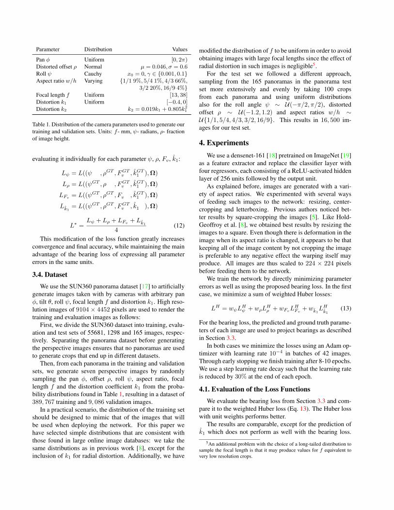
ψρ

Fv

k1

Projection Optimal Reg. Regression

Figure 6. Optimal selection of the weights when combining differ-ent loss components can greatly influence training. In gray, modelstrained with one weight in wψ, wρ, wFv , wk1 set to 100 and therest to 1. In red, a model trained with all weights set to 1. In green,a model trained with the bearing loss. These results indicate thatselecting appropriate weights is important for this task, but thatwith the proposed parameterization, selecting unit weights yieldsresults that are better than the proposed bearing loss.

However, that may not always be the case, for example,when using a different camera model, as reported by Yinet al. [13], or when using a different parameterization thanthe one we propose here. It just happens that this parameter-ization is well suited to be trained with unit weights. To il-lustrate the effect of selecting less optimal weights, we havetrained several networks using the weighted sum of Huberlosses (Eq. 13) with different sets of weights and comparethe resulting validation error curves in Figure 6.

For the rest of the paper, our approach or our networkrefer to a network trained by minimizing the proposed pa-rameters (Fv, k1, ρ, ψ) directly using a sum of Huber losses(Eq. 13) with wψ = wρ = wFv = wk1 = 1.

4.2. Effect of Distortion Parameterization

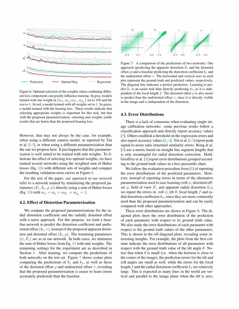
We compare the proposed parameterizations for the ra-dial distortion coefficient and the radially distorted offsetwith a naive approach. For this purpose, we train a base-line network to predict the distortion coefficient and undis-torted offset (k1, τ), instead of the proposed apparent distor-tion and distorted offset (k1, ρ). The remaining parameters(ψ, Fv) are as in our network. In both cases, we minimizethe sum of Huber losses from Eq. 13 with unit weights. Theremaining settings for the experiment are as described inSection 4. After training, we compare the predictions ofboth networks on the test set. Figure 7 shows scatter plotscomparing the predictions of k1 and k1, as well as thoseof the distorted offset ρ and undistorted offset τ , revealingthat the proposed parameterization is easier to learn (moreaccurately predicted) than the baseline.

-0.3 -0.1 -2.0 -1.0

k1 k1

-0.5 0.6 -0.5 0.6

τ ρ

Figure 7. A comparison of the predictions of two networks: Ourapproach (predicting the apparent distortion k1 and the distortedoffset ρ) and a baseline predicting the distortion coefficient k1 andthe undistorted offset τ . The horizontal and vertical axes in eachplot represent the ground truth and predicted values, respectively.The diagonal line indicates a perfect prediction. Learning to pre-dict k1 is an easier task than directly predicting k1, as it is inde-pendent of the focal length f . The distorted offset ρ is also easierto predict than the undistorted offset τ , since it is directly visiblein the image and is independent of the distortion.

4.3. Error Distributions

There is a lack of consensus when evaluating single im-age calibration networks: some previous works follow aclassification approach and directly report accuracy values[5]. Others establish a threshold on the regression errors andalso report accuracy values [8, 4]. Yin et al. [13] report peaksignal-to-noise ratio structural similarity errors. Rong et al.[6] use a metric based on straight line segment lengths thatis only meaningful for radial distortion correction. Hold-Geoffroy et al. [8] report error distributions grouped accord-ing to the ground truth values in a box-percentile chart.

We follow the evaluation procedure from [8] of reportingthe error distributions of the predicted parameters. How-ever, instead of reporting errors in terms of the alternativeparameterization used to ease learning (roll ψ, distorted off-set ρ, field of view Fv and apparent radial distortion k1),we report the errors in: roll ψ, tilt θ, focal length f and ra-dial distortion coefficient k1, since they are more commonlyused than the proposed parameterization and can be easilycompared with other approaches.

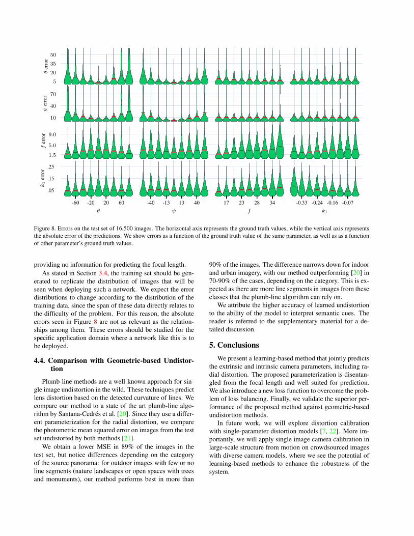
These error distributions are shown in Figure 8. The di-agonal plots show the error distribution of the predictionof each parameter with respect to its ground truth value.We also study the error distributions of each parameter withrespect to the ground truth values of the other parameters.This is shown in the off-diagonal plots, revealing some in-teresting insights. For example, the plots from the first col-umn indicate the error distributions of all parameters withrespect with the ground truth value of the tilt angle θ. No-tice that when θ is small (i.e. when the horizon is close tothe center of the image), the prediction errors for the tilt androll angles are small as well, while the errors for the focallength f and the radial distortion coefficient k1 are relativelylarge. This is expected as many lines in the world are ver-tical and parallel to the image plane when the tilt is zero,

5

20

35

50

θer

ror

10

40

70

ψer

ror

1.5

5.0

9.0

fer

ror

-60 -20 20 60θ

.05

.15

.25

k1

erro

r

-40 -13 13 40ψ

17 23 28 34f

-0.33 -0.24 -0.16 -0.07k1

Figure 8. Errors on the test set of 16,500 images. The horizontal axis represents the ground truth values, while the vertical axis representsthe absolute error of the predictions. We show errors as a function of the ground truth value of the same parameter, as well as as a functionof other parameter’s ground truth values.

providing no information for predicting the focal length.As stated in Section 3.4, the training set should be gen-

erated to replicate the distribution of images that will beseen when deploying such a network. We expect the errordistributions to change according to the distribution of thetraining data, since the span of these data directly relates tothe difficulty of the problem. For this reason, the absoluteerrors seen in Figure 8 are not as relevant as the relation-ships among them. These errors should be studied for thespecific application domain where a network like this is tobe deployed.

4.4. Comparison with Geometric-based Undistor-tion

Plumb-line methods are a well-known approach for sin-gle image undistortion in the wild. These techniques predictlens distortion based on the detected curvature of lines. Wecompare our method to a state of the art plumb-line algo-rithm by Santana-Cedres et al. [20]. Since they use a differ-ent parameterization for the radial distortion, we comparethe photometric mean squared error on images from the testset undistorted by both methods [21].

We obtain a lower MSE in 89% of the images in thetest set, but notice differences depending on the categoryof the source panorama: for outdoor images with few or noline segments (nature landscapes or open spaces with treesand monuments), our method performs best in more than

90% of the images. The difference narrows down for indoorand urban imagery, with our method outperforming [20] in70-90% of the cases, depending on the category. This is ex-pected as there are more line segments in images from theseclasses that the plumb-line algorithm can rely on.

We attribute the higher accuracy of learned undistortionto the ability of the model to interpret semantic cues. Thereader is referred to the supplementary material for a de-tailed discussion.

5. ConclusionsWe present a learning-based method that jointly predicts

the extrinsic and intrinsic camera parameters, including ra-dial distortion. The proposed parameterization is disentan-gled from the focal length and well suited for prediction.We also introduce a new loss function to overcome the prob-lem of loss balancing. Finally, we validate the superior per-formance of the proposed method against geometric-basedundistortion methods.

In future work, we will explore distortion calibrationwith single-parameter distortion models [7, 22]. More im-portantly, we will apply single image camera calibration inlarge-scale structure from motion on crowdsourced imageswith diverse camera models, where we see the potential oflearning-based methods to enhance the robustness of thesystem.

References[1] R. Hartley and A. Zisserman, Multiple view geometry in

computer vision. Cambridge university press, 2003. 1

[2] B. Caprile and V. Torre, “Using vanishing points for cameracalibration,” International Journal of Computer Vision,vol. 4, no. 2, pp. 127–139, mar 1990. [Online]. Available:https://doi.org/10.1007/BF00127813 1

[3] J. Deutscher, M. Isard, and J. MacCormick, “AutomaticCamera Calibration from a Single Manhattan Image,” inComputer Vision — ECCV 2002, A. Heyden, G. Sparr,M. Nielsen, and P. Johansen, Eds. Berlin, Heidelberg:Springer Berlin Heidelberg, 2002, pp. 175–188. 1

[4] S. Workman, C. Greenwell, M. Zhai, R. Baltenberger, andN. Jacobs, “DEEPFOCAL: A method for direct focal lengthestimation,” in 2015 IEEE International Conference on Im-age Processing (ICIP), sep 2015, pp. 1369–1373. 2, 3, 7

[5] S. Workman, M. Zhai, and N. Jacobs, “Horizon Linesin the Wild,” pp. 1–12, 2016. [Online]. Available:http://arxiv.org/abs/1604.02129 2, 3, 6, 7

[6] J. Rong, S. Huang, Z. Shang, and X. Ying, “Radial LensDistortion Correction Using Convolutional Neural NetworksTrained with Synthesized Images,” in Computer Vision –ACCV 2016, S.-H. Lai, V. Lepetit, K. Nishino, and Y. Sato,Eds. Cham: Springer International Publishing, 2017, pp.35–49. 2, 7

[7] A. W. Fitzgibbon, “Simultaneous linear estimation of multi-ple view geometry and lens distortion,” in Computer Visionand Pattern Recognition, 2001. CVPR 2001. Proceedingsof the 2001 IEEE Computer Society Conference on, vol. 1.IEEE, 2001, pp. I–I. 2, 8

[8] Y. Hold-Geoffroy, K. Sunkavalli, J. Eisenmann, M. Fisher,E. Gambaretto, S. Hadap, and J.-F. Lalonde, “A PerceptualMeasure for Deep Single Image Camera Calibration,”2018 IEEE Conference on Computer Vision and PatternRecognition (CVPR), 2018. [Online]. Available: http://arxiv.org/abs/1712.01259 2, 3, 6, 7

[9] M. Zhai, S. Workman, and N. Jacobs, “Detecting VanishingPoints Using Global Image Context in a Non-ManhattanWorld,” 2016 IEEE Conference on Computer Visionand Pattern Recognition (CVPR), pp. 5657–5665, 2016.[Online]. Available: http://ieeexplore.ieee.org/document/7780979/ 2

[10] R. Caruana, “Multitask learning,” Machine learning, vol. 28,no. 1, pp. 41–75, 1997. 2

[11] A. Kendall, Y. Gal, and R. Cipolla, “Multi-task learning us-ing uncertainty to weigh losses for scene geometry and se-mantics,” in Proceedings of the IEEE Conference on Com-puter Vision and Pattern Recognition (CVPR), 2018. 2

[12] Z. Chen, V. Badrinarayanan, C.-Y. Lee, and A. Rabi-novich, “GradNorm: Gradient normalization for adaptiveloss balancing in deep multitask networks,” arXiv preprintarXiv:1711.02257, 2017. 2

[13] X. Yin, X. Wang, J. Yu, M. Zhang, P. Fua, and D. Tao,“FishEyeRecNet: A Multi-Context Collaborative DeepNetwork for Fisheye Image Rectification,” pp. 1–16, 2018.[Online]. Available: http://arxiv.org/abs/1804.04784 2, 7

[14] B. Triggs, P. F. McLauchlan, R. I. Hartley, and A. W. Fitzgib-bon, “Bundle adjustment—a modern synthesis,” in Interna-tional workshop on vision algorithms. Springer, 1999, pp.298–372. 4

[15] P. Sturm and S. Ramalingam, “A Generic Concept forCamera Calibration,” in 8th European Conference onComputer Vision (ECCV ’04), ser. Lecture Notes inComputer Science (LNCS), J. Matas and T. Pajdla, Eds.,vol. 3022/2004. Prague, Czech Republic: Springer-Verlag, May 2004, pp. 1–13. [Online]. Available: https://hal.inria.fr/inria-00524411 5

[16] S. Ramalingam, S. K. Lodha, and P. Sturm, “A genericstructure-from-motion framework,” Computer Vision andImage Understanding, vol. 103, no. 3, pp. 218–228, 2006.[Online]. Available: https://hal.inria.fr/inria-00384319 5

[17] J. Xiao, K. A. Ehinger, A. Oliva, and A. Torralba, “Recogniz-ing scene viewpoint using panoramic place representation,”in Computer Vision and Pattern Recognition (CVPR), 2012IEEE Conference on. IEEE, 2012, pp. 2695–2702. 6

[18] G. Huang, Z. Liu, L. Van Der Maaten, and K. Q. Wein-berger, “Densely connected convolutional networks.” inCVPR, vol. 1, no. 2, 2017, p. 3. 6

[19] O. Russakovsky, J. Deng, H. Su, J. Krause, S. Satheesh,S. Ma, Z. Huang, A. Karpathy, A. Khosla, M. Bernstein,A. C. Berg, and L. Fei-Fei, “ImageNet Large Scale VisualRecognition Challenge,” International Journal of ComputerVision (IJCV), vol. 115, no. 3, pp. 211–252, 2015. 6

[20] D. Santana-Cedres, L. Gomez, M. Aleman-Flores, A. Sal-gado, J. Escların, L. Mazorra, and L. Alvarez, “An iterativeoptimization algorithm for lens distortion correction usingtwo-parameter models,” Image Processing On Line, vol. 6,pp. 326–364, 2016. 8

[21] R. Szeliski, “Prediction error as a quality metric for motionand stereo,” in Proceedings of the Seventh IEEE Interna-tional Conference on Computer Vision, vol. 2, Sep. 1999,pp. 781–788 vol.2. 8

[22] C. Ishii, Y. Sudo, and H. Hashimoto, “An image conversionalgorithm from fish eye image to perspective image for hu-man eyes,” in Advanced Intelligent Mechatronics, 2003. AIM2003. Proceedings. 2003 IEEE/ASME International Confer-ence on, vol. 2. IEEE, 2003, pp. 1009–1014. 8