Data Sources and Computational Approaches for Generating Models of

1

Data Sources and Computational Approaches for Generating Models of

Gene Regulatory Networks

B. D. Aguda,1 G. Craciun,2 R. Cetin-Atalay3

1 Department of Genetics and Genomics, Boston University School of Medicine

715 Albany Street, Boston, Massachusetts, USA 02118

2 Mathematical Biosciences Institute, The Ohio State University

231 W. 18th Avenue, Columbus, Ohio, USA 43210

3 Department of Molecular Biology & Genetics, Bilkent University, Ankara, Turkey

and Virginia Bioinformatics Institute, Virginia Polytechnic Institute and State

University, Blacksburg,Virgina,USA 24061

2

OUTLINE

Introduction

Formal representation of GRNs

An example of a GRN: The Lac Operon

Hierarchies of GRN models: From probabilistic graphs to mechanistic models

A guide to databases and knowledgebases on the internet

Pathway Databases & Platforms

Ontologies for GRN modeling

Current Gene, Interaction, and Pathway Ontologies

Whole-cell modeling platforms

Ontology for modeling multi-scale and incomplete networks

An ontology for cellular processes

The PATIKA pathway ontology

Extracting Models from Pathways Databases

Pathway and Dynamic Analysis Tools for GRNs

Global network properties

Recurring network motifs

Identifying pathway channels in networks: extreme pathway analysis

Network stability analysis

Predicting dynamics & bistability from network structure alone

Concluding Remarks

3

INTRODUCTION

High-throughput data acquisition technologies in molecular biology, including

rapid DNA sequencers, gene expression microarrays and other microchip-based assays,

are providing an increasingly comprehensive parts list of a biological cell. Although this

parts list may be far from complete at this time, the so-called “post-genomic era” has now

begun in which the goal is to integrate the parts and analyze how they interact to

determine the system’s behavior. This integration is being facilitated by the creation of

databases, knowledgebases and other information repositories on the internet. How these

huge amounts of information will be used to answer biological questions and predict

behavior will keep multidisciplinary teams of scientists busy for many years. A key

question is how the expression of genes is regulated in response to various intracellular

and external conditions and stimuli. The current paradigm is that the secret to life could

be found in the genetic code; however, the expression of genes and the unfolding of the

regulatory molecular networks in response to the environment may well be the defining

attribute of the living state.

This chapter focuses on gene regulatory networks (GRNs). A “gene regulatory

network” refers to a set of molecules and interactions that affect the expression of genes

located in the DNA of a cell. Gene expression is the combination of transcription of

DNA sequences, processing of the primary RNA transcripts, and translation of the

mature messenger RNA (mRNA) to proteins in ribosomes. This picture is often referred

to as the “central dogma” and it has been the canonical model for the flow of information

from the genetic code to proteins. These processes are shown schematically as steps

labeled τ , ρ and σ in Fig 1.

4

Figure 1. A schematic representation of a gene regulatory network involving

modules of molecular classes (shown in boxes); the modules shown are the

transcriptional units in the genome (G), primary transcripts (Ro), mature

transcripts (R), primary proteins (Po), modified proteins (P), and metabolites (M).

The labeled steps shown in black lines are transcription (τ), RNA processing (ρ),

translation (σ), protein modification (µ), metabolic pathways (π), and genome

replication (α). The feedback interactions shown in gray lines are discussed in

the text. Filled circles represent either inhibition or activation.

5

The step labeled µ in Fig 1 represents modification of primary proteins to render

them functional; examples would be post-translational covalent modifications (e.g.

phosphorylation) and binding with other proteins or other molecules. Represented within

the set of steps µ are the many regulatory events (other than transcription and translation)

affecting gene expression and the overall physiology of the cell.

The complexity of GRNs may arise from the many possible feedback loops

shown as gray lines in Fig 1. In step τ , proteins could be directly involved in

transcription, as in the case of transcription factors binding to upstream regulatory

regions of genes. Many RNA and protein molecules cooperate in the translation step σ

in Fig 1; examples are tRNA, rRNA, and ribosomal proteins.

The first goal of this chapter is to survey sources of data and other information

that can be used to generate models of GRNs. The focus is on biological databases and

knowledgebases that are available on the internet, especially those that attempt to

integrate heterogeneous information including molecular interactions and pathways. The

second goal of this review is to summarize current models of GRNs and how they can be

extracted from biological databases. Depending on the nature of the data, different

granularities of GRN models can be generated, ranging from probabilistic graphical

models to detailed kinetic or mechanistic models. A crucial issue in the design of

pathways databases is how to represent information having various levels of uncertainty.

Because of its central importance in GRN modeling, an extensive discussion of pathway

ontology is given. Lastly, the third goal is to discuss theoretical and computational

methods for the analysis of detailed models of GRNs. In particular, a summary is given

6

of various tools already developed in the field of reaction network analysis. Particular

emphasis of the discussion is on exploiting information on network structure to deduce

potential behavior of GRNs without knowing quantitative values of rate parameters.

FORMAL REPRESENTATION OF GRNS

The GRN of Fig 1 can be formally translated to a set of general dynamical

equations. The modules (in boxes) in the GRN represent the following classes of

biomolecules:

G : vector of all transcriptional units (TUs) involved in the GRN (in terms, for

example, of gene dosage per TU);

Ro : vector of primary RNA transcripts corresponding to the TUs in G;

R : vector of messenger RNA (mRNA), transfer RNA (tRNA), ribosomal

RNA (rRNA), and other processed RNAs;

Po : vector of newly translated (primary) proteins;

P : vector of modified proteins;

M : vector of metabolites.

Disregarding the replication of the genomic DNA (step α) and the changes in the

metabolome M for now (i.e. assume G and M to be constant), a mathematical

representation of the dynamics of the GRN in Fig 1 would be the following set of vector-

matrix equations:

7

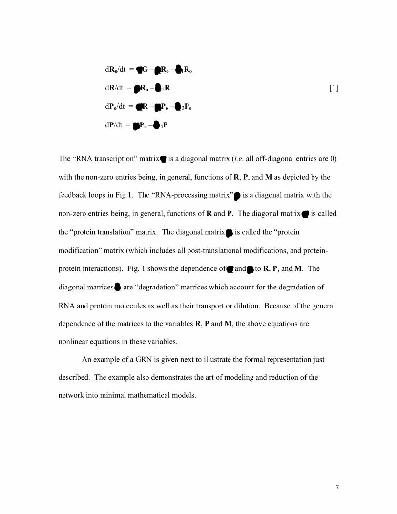
dRo/dt = τG – ρRo – δ1Ro

dR/dt = ρRo – δ 2R [1]

dPo/dt = σR – µPo – δ 3Po

dP/dt = µPo – δ 4P

The “RNA transcription” matrix τ is a diagonal matrix (i.e. all off-diagonal entries are 0)

with the non-zero entries being, in general, functions of R, P, and M as depicted by the

feedback loops in Fig 1. The “RNA-processing matrix” ρ is a diagonal matrix with the

non-zero entries being, in general, functions of R and P. The diagonal matrix σ is called

the “protein translation” matrix. The diagonal matrix µ is called the “protein

modification” matrix (which includes all post-translational modifications, and protein-

protein interactions). Fig. 1 shows the dependence of σ and µ to R, P, and M. The

diagonal matrices δ i are “degradation” matrices which account for the degradation of

RNA and protein molecules as well as their transport or dilution. Because of the general

dependence of the matrices to the variables R, P and M, the above equations are

nonlinear equations in these variables.

An example of a GRN is given next to illustrate the formal representation just

described. The example also demonstrates the art of modeling and reduction of the

network into minimal mathematical models.

8

AN EXAMPLE OF A GRN: THE LAC OPERON

The lac operon in the bacterium Escherichia coli is a well-studied GRN. This

prokaryotic gene network has been the subject of numerous reviews;1-4 it is discussed

here primarily to illustrate the various aspects of GRN modeling, starting with the

information on genome organization (operon structure) to knowledge on protein-DNA

interactions, protein-protein interactions and the influence of metabolites.

Understanding the lac operon begins by looking at the genome organization of E.

coli. The complete genome sequence of various strains of this bacterium can be accessed

through the webpage of the National Center for Biotechnology Information

(http://www.ncbi.nlm.nih.gov). From the homepage menu, clicking Entrez followed by

Genome gives the link to complete bacterial genomes including E. coli. Genes in the

circular chromosome of E. coli are organized into ‘operons’. An operon is a cluster of

genes whose expression is controlled by a common set of operator sequences and

regulatory proteins.5 The genes in the cluster are usually involved in the synthesis of

enzymes needed for the metabolism of a molecule. Several reviews on the influence of

operon structure on the dynamical behavior of GRNs are available.6-7

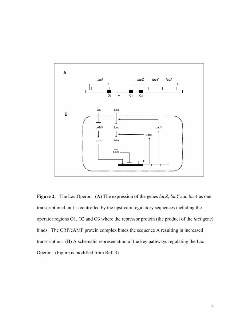
The lac operon is shown in Fig 2A. The GRN involves the gene set

{lacZ, lacY, lacA, lacI} and the regulatory sequences {O1, O2, O3, A} as shown in Fig

2A. The gene lacI encodes a repressor protein that binds the operator sequences O1,

9

Figure 2. The Lac Operon. (A) The expression of the genes lacZ, lacY and lacA as one

transcriptional unit is controlled by the upstream regulatory sequences including the

operator regions O1, O2 and O3 where the repressor protein (the product of the lacI gene)

binds. The CRP/cAMP protein complex binds the sequence A resulting in increased

transcription. (B) A schematic representation of the key pathways regulating the Lac

Operon. (Figure is modified from Ref. 3).

10

O2, and O3 thereby repressing the synthesis of the lacZ-lacY-lacA transcript. Gene lacZ

encodes the β-galactosidase enzyme, gene lacY encodes a permease, and gene lacA

encodes a transacetylase. The CRP/cAMP complex binds the sequence A and enhances

transcription.

The key pathways that generate the switching behavior of the GRN are shown in

Fig 2B. This switching behavior of the lac operon explains the diauxic growth (shift

from glucose to lactose utilization) of E. coli. If there is glucose in the growth medium,

the operon is always OFF because glucose inhibits cAMP and lactose transport into the

cell. If glucose is absent, the operon would remain OFF unless some lactose is present

inside the cell (which is true when glucose is depleted and lactose from the outside can

now enter the cell); an initially small amount of internal lactose increases rapidly due to

at least two positive feedback loops as shown in Fig 2B. It is the positive feedback loop

involving lactose transport that ultimately controls the influx of lactose.

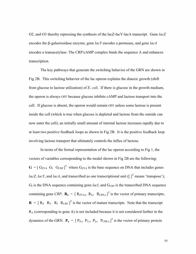
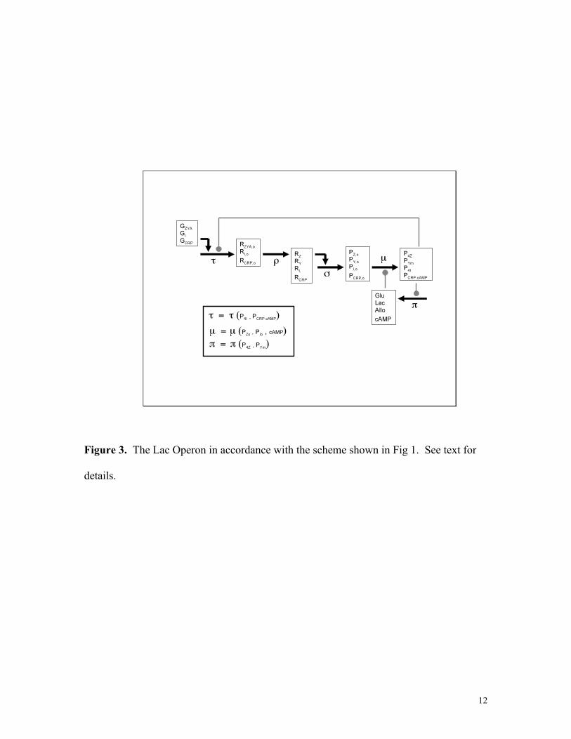
In terms of the formal representation of the lac operon according to Fig 1, the

vectors of variables corresponding to the model shown in Fig 2B are the following:

G = [ GZYA GI GCRP ]T where GZYA is the base sequence on DNA that includes genes

lacZ, lacY, and lacA, and transcribed as one transcriptional unit ([ ]T means ‘transpose’);

GI is the DNA sequence containing gene lacI, and GCRP is the transcribed DNA sequence

containing gene CRP. Ro = [ RZYA,o RI,o RCRP,o ]T is the vector of primary transcripts;

R = [ RZ RY RI RCRP ]T is the vector of mature transcripts. Note that the transcript

RA (corresponding to gene A) is not included because it is not considered further in the

dynamics of the GRN. Po = [ PZ,o PY,o PI,o PCRP,o ]T is the vector of primary protein

11

translates; P = [ P4Z PYm P4I PCRP.cAMP ]T is the vector of mature, modified, and

active proteins; the protein PZ (β-galactosidase) is tetrameric in its functional form, the

permease PY acts at the plasma membrane (hence the subscript ‘m’ in PYm), the repressor

protein PI is tetrameric, and CRP’s binding with cAMP is necessary for its DNA-binding

activity. M = [ Glu Lac Allo cAMP ]T is the vector of metabolites (Glu = glucose,

Lac = lactose, Allo = allolactose, cAMP = cyclic adenosine monophosphate). The GRN

for the lac operon model using the representation of Fig 1 is shown in Fig 3. The first

equation in [1] would look like this:

[2]

where τ11 would be a function of PI and PCRP.cAMP. For example, one could choose the

function τ11 = (c1+c2PCRP.cAMP)/(c3+c4PIn) to represent the activation of transcription by

the protein complex PCRP.cAMP and inhibition by the tetrameric repressor PI (the n and ci’s

are constant parameters; n should be greater than 1 because of the tetrameric complex of

PI).

12

Figure 3. The Lac Operon in accordance with the scheme shown in Fig 1. See text for

details.

13

New mathematical models and reviews on the lac operon have appeared

recently.2-4 Yildirim and Mackey2 used delay differential equations to account for the

transcriptional and translational steps that are missing in their model. An earlier detailed

kinetic model was proposed and analyzed by Wong, Gladney and Keasling.1 Recently,

Vilar, Guet, and Leibler4 used a 4-variable model that captures many of the essential

dynamics of the lac operon. Note that the Vilar-Guet-Leibler model is essentially a three-

variable model. The bistability exhibited by the model was used as the explanation for

the ON-OFF behavior of the lac operon.

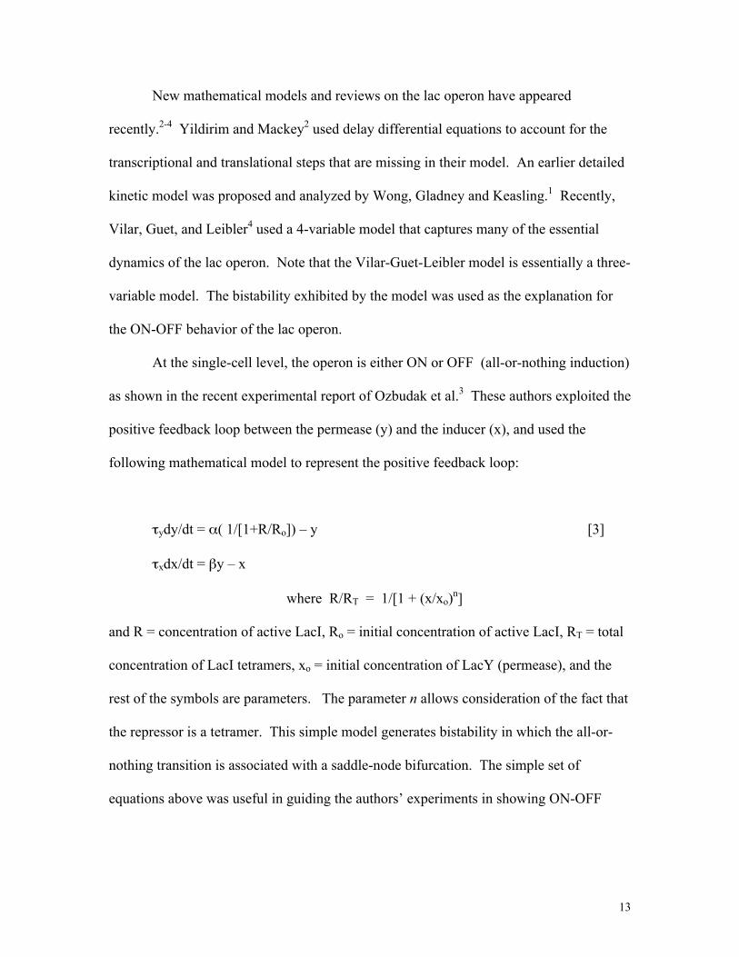
At the single-cell level, the operon is either ON or OFF (all-or-nothing induction)

as shown in the recent experimental report of Ozbudak et al.3 These authors exploited the

positive feedback loop between the permease (y) and the inducer (x), and used the

following mathematical model to represent the positive feedback loop:

τydy/dt = α( 1/[1+R/Ro]) – y [3]

τxdx/dt = βy – x

where R/RT = 1/[1 + (x/xo)n]

and R = concentration of active LacI, Ro = initial concentration of active LacI, RT = total

concentration of LacI tetramers, xo = initial concentration of LacY (permease), and the

rest of the symbols are parameters. The parameter n allows consideration of the fact that

the repressor is a tetramer. This simple model generates bistability in which the all-or-

nothing transition is associated with a saddle-node bifurcation. The simple set of

equations above was useful in guiding the authors’ experiments in showing ON-OFF

14

behavior as well exploring the phase diagram (coordinates of which are the variables x

and y, for example) for bistable and monostable regions.

The lac operon illustrates several important points in modeling GRNs. Although

the operon structure is not a general property of all genomes, one can expect that genomic

DNA sequence organization affects the dynamics of the GRN; this is primarily due to

co-expression of genes found in the same transcriptional units or co-regulation of genes

by transcription factors that recognize promoter regions having similar regulatory

sequences. Another lesson from the lac operon is that abstraction of the complex GRN

may be sufficient to understand the behavior of the system. This abstraction was

facilitated by prior knowledge of the influence of network topology on dynamical

behavior, e.g. bistability arising from positive feedback loops.8 A discussion on how

network structure alone influences system behavior is provided in the penultimate section

of this chapter.

HIERARCHIES OF GRN MODELS: FROM PROBABILISTIC GRAPHS TO

DETERMINISTIC MODELS

The general representation of GRNs in Fig 1 considers groups of molecules

according to their chemical classes (DNA, RNA, proteins, metabolites) whose

“interactions” merely encode the broad concepts of transcription, post-transcriptional

processing, translation and post-translational modifications. Depending on the nature of

15

available experimental information, specific models of gene regulatory networks can be

constructed at various levels of detail.

Networks, in general, are described by their graphical structures. A graph is

basically a set of ‘nodes’ and a set of ‘edges’, the latter being the representations of the

interactions or associations among nodes. Progressively more detailed mechanistic

information can be added to a graph as they become available. At one extreme of the

spectrum of models, the nodes in the graph could be just a set of genes (and no other

kinds of objects), with certain pairs of genes linked by undirected edges if these pairs are

known to “interact” or are “associated” in some way. Sometimes the nodes could be

proteins and the edges represent physical interactions. Because of the correspondence

between proteins and genes (albeit not generally one-to-one), protein-protein interaction

networks may imply some underlying GRN structure. In general, nodes in a graph can be

defined according to the level of detail that is sufficient to describe a particular feature,

function or behavior of the system. For example, the nodes in Fig 1 represent various

classes of molecules. A node could also represent a subnetwork or module with specific

cellular function.

An edge of a graph is assigned a direction if there is information on causality, i.e.

that one node affects the state of the other. A directed edge can be further characterized

as either “activating” or “inhibiting”. As more quantitative data are available, it may be

possible to identify the “strength” of an edge. For dynamic models, the strength of an

edge would, for example, require identification of rate expressions as functions of the

states of the nodes. At this point, a dynamic model encoded in deterministic differential

equations is possible. Finally, at the other extreme in the spectrum of GRN models,

16

microscopic details of the interactions between individual molecular species are known

and molecular dynamic simulations are possible.

As the example of the lac operon illustrates, abstract models involving differential

equations that do not necessarily reflect the detailed mechanism are sometimes used

when the goal is primarily to explore possible system dynamics arising from the structure

of the network. Associated with the process of ‘abstraction’ is the problem of reducing

the network into a smaller set of ‘modules’ and their interactions. Modules can range

from individual molecules or genes, to a set of genes or proteins, or to functional

subnetworks with definable cellular functions. Similar ideas have been discussed

recently by Vilar et al.4 in their work on the lac operon. The lac operon is an example of

a well-defined small model system in which a considerable amount of biological

knowledge and mechanistic understanding have already accumulated so that refined

mathematical modeling can be carried out. Many other focused models and

corresponding mathematical model formalisms have been reviewed recently by de Jong.9

In contrast, constructing the network graph of gene interactions from large-scale gene

expression measurements is just beginning and is, at times, controversial. Since this field

has been reviewed10-13 recently only a brief account is given below.

High-throughput gene expression measurements using DNA microarrays provide

global snapshots of the dynamics of gene networks at the RNA level. Expression data are

intrinsically noisy and conclusions derived from them are probabilistic in nature.

Furthermore, the mRNA levels are averages from cell populations. Gene network

reconstruction from microarray data also suffers from the so-called ‘dimensionality

problem’11 because the number of genes is much greater than the number of microarray

17

experiments. Statistical analysis of gene expression data usually employ clustering

methods to find genes with similar expression patterns across time series or across

different experimental conditions (e.g. see Refs. 14-15). The assumption is that clustered

or co-expressed genes are somehow co-regulated or perhaps share similar functions. The

results of clustering in terms of GRN modeling could therefore be a coarse-grain network

composed of modules (nodes), each module representing a set of genes with similar

functions.

Graphical models that combine probability theory and graph theory are suitable

frameworks for inferring GRNs from gene expression data.10, 16 In general, these

graphical models are probability models for multivariate random variables whose

independence structure can be represented by a conditional independence graph.

Recently, Friedman10 reviewed the field of probabilistic graphical models for gene

networks, including Bayesian networks. In a Bayesian network, the nodes represent

random variables (e.g. genes and their expression levels) while the edges show

conditional dependence relations. Husmeier17-18 has also reviewed the applications of

Bayesian networks to microarray data. Bayesian networks were first applied to the

problem of reverse engineering of GRNs from microarray expression data by Friedman et

al.,19 Pe’er et al.,20 and Hartemink et al.21 Other examples of graphical models employing

various statistical methods are discussed by Wang, Myklebost and Hovig.16

Zak et al.22 have argued that inferring the GRN structure from expression data

alone is impossible. However, promising results come from more recent work showing

that properly designed perturbation experiments do permit network reconstruction (see

Refs. 12, 13, 18, 23-25). Two papers23-24 extended ideas from metabolic control analysis

18

to suggest perturbation experiments designed to determine the direction and strengths of

interactions between genes. Also, Gardner et al.25 used systematic perturbations

combined with least-squares regression to infer the gene network topology and weights of

interactions.

In general, the issues encountered during the creation of a GRN graph are similar

to those faced when designing a pathway or interaction database. These issues will be

discussed in more detail in the section on ‘pathway ontology’ below. An extensive

discussion on this ontology is provided because it is a crucial stepping stone for future

projects concerned with the extraction of GRN models from pathways databases.

Pathways databases are relatively recent developments in bioinformatics. These

databases are built from more elementary databases and it is important to be aware of the

many heterogeneous bioinformatics resources available, most of them on the internet.

Thus, a brief guide is given next.

A GUIDE TO DATABASES AND KNOWLEDGEBASES ON THE INTERNET

The field of bioinformatics has naturally arisen to cope with the deluge of data

generated by high-throughput technologies in genomics, transcriptomics, proteomics, and

other –omics. These data are organized into databases (DBs) and knowledgebases (KBs),

many of which are publicly available on the internet. Comprehensive and realistic

modeling of GRNs should tap into the information contained in these DBs and KBs.

Thus, it is expected that the next generation of modelers will have to be sufficiently

19

aware of bioinformatics resources. It is for this reason that an overview of the major

bioinformatics DBs and KBs is provided here, although their utility for modeling GRNs

may not be direct and obvious at this time. It was alluded to in the discussion of the lac

operon that understanding the operon structure of the genomic DNA was necessary to

understand the dynamics of the network. In general, relating genome organization to

GRN dynamics is a very difficult and still a very much open problem. This section

begins with genomic sequence databases in anticipation of their future use in helping

predict GRN structures; a specific example would be that of finding regulatory sequences

where transcription factors bind thereby linking one gene product to the transcription of

another gene.

To date, the genomes of more than 150 organisms have been sequenced, and

many more sequencing projects are currently going on or planned. Publicly available

DNA sequence data as well as functional and structural data on proteins are accumulating

at an exponential rate, virtually doubling every year. The major sequence and structure

repositories which are regularly updated are listed in Table 1.

20

Table 1. Major sequence and structure repositories

Database Description URL

GenBank Repository of all publicly available annotated nucleotide and protein sequences http://www.ncbi.nlm.nih.gov/

EMBL Database Repository of all publicly available annotated nucleotide and protein sequences http://www.ebi.ac.uk/embl.html

DDBJ (DNA Data Bank of Japan)

Repository of all publicly available annotated nucleotide and protein sequences http://www.ddbj.nig.ac.jp

PIR Protein information resource: protein sequence database http://pir.georgetown.edu/

Swiss-Prot Highly annotated curated protein sequence database http://www.expasy.org/sprot

PDB Protein structure databank: Collection of publicly available 3D structures of proteins and nucleic acids http://www.rcsb.org/pdb

Table 2. Protein sequence and structure property databases

Database Description URL

eMOTIF Protein sequence motif database http://motif.stanford.edu/emotif InterPro Integrated resource of protein families, domains http://www.ebi.ac.uk/interpro iProClass Integrated protein classification database http://pir.georgetown.edu/iproclass/ ProDom Protein domain families http://www.toulouse.inra.fr/prodom.html

CDD Conserved domain database: covers protein domain information from Pfam, SMART and COG databases

http://www.ncbi.nlm.nih.gov/Structure/cdd/cdd.shtml

CATH Protein structure classification database http://www.biochem.ucl.ac.uk/bsm/cath/ CE Repository of 3D Protein structure alignments http://cl.sdsc.edu/ce.html SCOP Structural classification of proteins http://scop.mrc-lmb.cam.ac.uk/scop

21

The partners of the International Nucleotide Sequence Databases (INSD), namely

GenBank, EMBL and DDBJ, share their nucleic acid sequence data for a comprehensive

coverage of all available genome information. Swiss-Prot is a manually curated protein

sequence database with a high level annotation of protein function and protein

modifications, including links to property, structure and pathways databases. PIR is

similar to Swiss-Prot, with the former providing some options for sequence analysis.

Recently, UniProt Knowledgebase (http://www.uniprot.org) was established with the aim

of unifying and linking protein databases with cross-references and query options.

Some of the major protein sequence and structure property databases are listed in

Table 2. Although there are many more general or specialized property databases

available,26 the list given in Table 2 is a good start for exploring protein property

databases. Table 3 gives a list of gene expression repositories.

It is very difficult for one person to keep up with the rapidly increasing number of

genomics, proteomics, and interactomics and metabolomics databases, let alone their

intended usage.26 To alleviate this problem, an increasing number of integrated database

retrieval and analysis systems tools are being developed for the purpose of data

management, acquisition, integration, visualization, sharing and analysis. Table 4 lists

promising examples of these tools, which are regularly maintained and updated.

GeneCards is an integrated database of human genes, genomic maps, proteins, and

diseases, with software that retrieves, combines, searches, and displays human genome

information. GenomNet is of particular interest since its analytical tools are

22

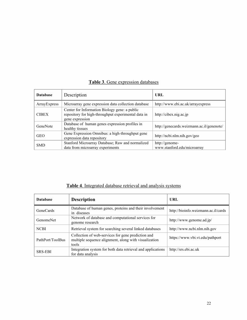
Table 3. Gene expression databases

Database Description URL

ArrayExpress Microarray gene expression data collection database http://www.ebi.ac.uk/arrayexpress

CIBEX Center for Information Biology gene: a public repository for high-throughput experimental data in gene expression

http://cibex.nig.ac.jp

GeneNote Database of human genes expression profiles in healthy tissues http://genecards.weizmann.ac.il/genenote/

GEO Gene Expression Omnibus: a high-throughput gene expression data repository http://ncbi.nlm.nih.gov/geo

SMD Stanford Microarray Database; Raw and normalized data from microarray experiments

http://genome-www.stanford.edu/microarray

Table 4. Integrated database retrieval and analysis systems

Database Description URL

GeneCards Database of human genes, proteins and their involvement in diseases http://bioinfo.weizmann.ac.il/cards

GenomeNet Network of database and computational services for genome research http://www.genome.ad.jp/

NCBI Retrieval system for searching several linked databases http://www.ncbi.nlm.nih.gov

PathPort/ToolBus Collection of web-services for gene prediction and multiple sequence alignment, along with visualization tools

https://www.vbi.vt.edu/pathport

SRS-EBI Integration system for both data retrieval and applications for data analysis

http://srs.ebi.ac.uk

23

tightly linked with the KEGG pathways database (discussed in the next section). ToolBus

comprises several data analysis software platforms such as multiple sequence alignment,

phylogenetic trees, generic XML viewer, pathways and microarray analysis, which are

linked to each other as well as to major databases. SRS and NCBI serve as general data

retrieval portals as well as to provide links to specific analysis tools.

PATHWAYS DATABASES AND PLATFORMS

Along with recent advances in genomics and proteomics, requirements for

analysis, expansion and visualization of cell signaling, GRNs and protein-protein

interaction maps are leading to the development of data representation and integration

tools. Pathways databases can be classified into four groups according to their

interactome data content and representation as listed in Table 5. Only those websites that

are regularly maintained are included in the list. The first group of databases represents

binary interaction databases. BIND, DIP, and MINT document experimentally

determined protein-protein interactions from peer-reviewed literature or from other

curated databases. BIND and MINT store experimental conditions used to observe the

interaction, chemical action, kinetics and other information linked to the original research

articles.

Static image databases are very good sources of pathway diagrams which provide

a broad introductory view of cell regulatory pathways along with good reviews and links.

24

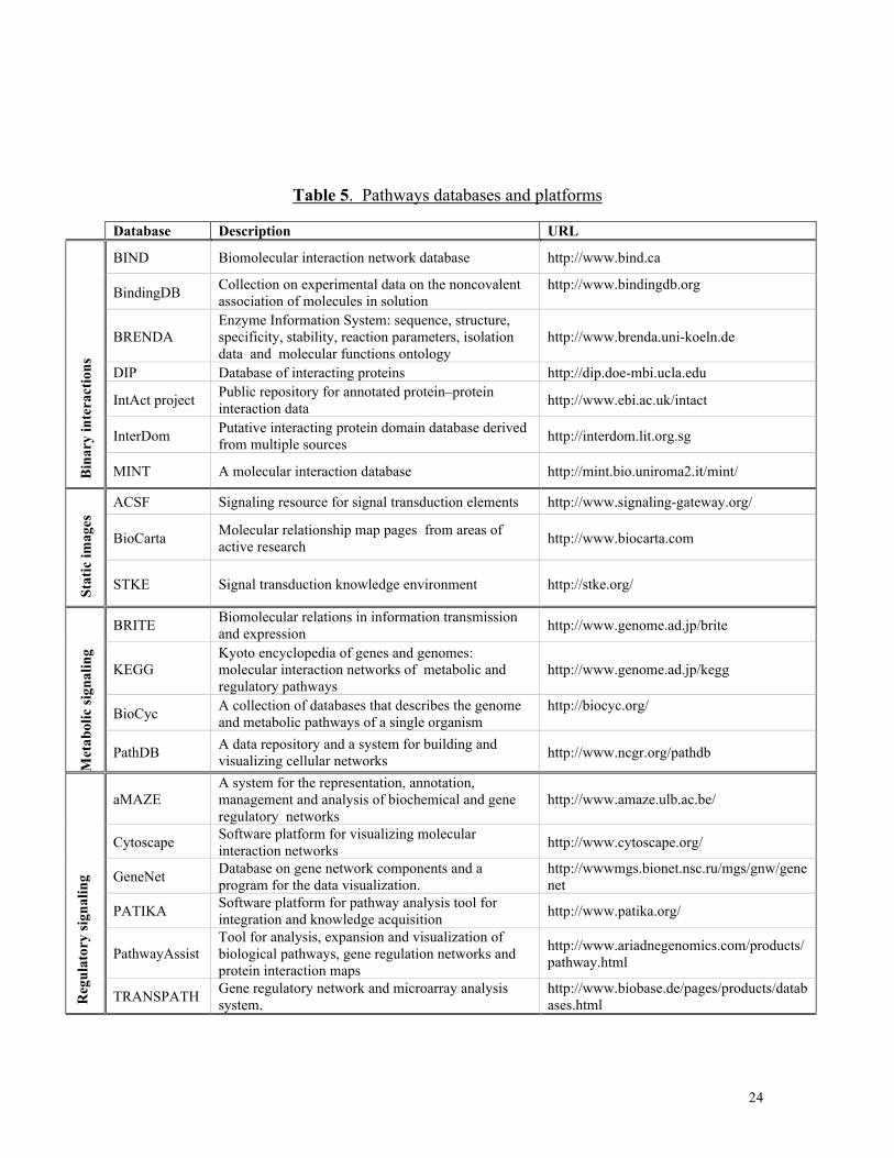
Table 5. Pathways databases and platforms

Database Description URL

BIND Biomolecular interaction network database http://www.bind.ca

BindingDB Collection on experimental data on the noncovalent association of molecules in solution

http://www.bindingdb.org

BRENDA Enzyme Information System: sequence, structure, specificity, stability, reaction parameters, isolation data and molecular functions ontology

http://www.brenda.uni-koeln.de

DIP Database of interacting proteins http://dip.doe-mbi.ucla.edu

IntAct project Public repository for annotated protein–protein interaction data http://www.ebi.ac.uk/intact

InterDom Putative interacting protein domain database derived from multiple sources http://interdom.lit.org.sg

Bin

ary

inte

ract

ions

MINT A molecular interaction database http://mint.bio.uniroma2.it/mint/

ACSF Signaling resource for signal transduction elements http://www.signaling-gateway.org/

BioCarta Molecular relationship map pages from areas of active research http://www.biocarta.com

Stat

ic im

ages

STKE Signal transduction knowledge environment http://stke.org/

BRITE Biomolecular relations in information transmission and expression http://www.genome.ad.jp/brite

KEGG Kyoto encyclopedia of genes and genomes: molecular interaction networks of metabolic and regulatory pathways

http://www.genome.ad.jp/kegg

BioCyc A collection of databases that describes the genome and metabolic pathways of a single organism

http://biocyc.org/

Met

abol

ic si

gnal

ing

PathDB A data repository and a system for building and visualizing cellular networks http://www.ncgr.org/pathdb

aMAZE A system for the representation, annotation, management and analysis of biochemical and gene regulatory networks

http://www.amaze.ulb.ac.be/

Cytoscape Software platform for visualizing molecular interaction networks http://www.cytoscape.org/

GeneNet Database on gene network components and a program for the data visualization.

http://wwwmgs.bionet.nsc.ru/mgs/gnw/genenet

PATIKA Software platform for pathway analysis tool for integration and knowledge acquisition http://www.patika.org/

PathwayAssist Tool for analysis, expansion and visualization of biological pathways, gene regulation networks and protein interaction maps

http://www.ariadnegenomics.com/products/pathway.html

Reg

ulat

ory

sign

alin

g

TRANSPATH Gene regulatory network and microarray analysis system.

http://www.biobase.de/pages/products/databases.html

25

ACSF, STKE and Biocarta are comprehensive knowledgebases on signal transduction

pathways and other regulatory networks.

Metabolic signaling databases contain detailed information on metabolic

pathways. These DBs have well established data structures but have non-uniform

ontologies. BioCyc is a collection of pathway/genome databases for many bacteria and

up to 14 species of other organisms. Enzyme catalyzed reactions, or the gene that

encodes that enzyme or the structures of chemical compounds in pathways and reactions,

can be displayed by BioCyc ontology based software for a given biochemical pathway.

In addition BioCyc supports computational tools for simulation of metabolic pathways.

KEGG is a frequently (daily) updated group of databases for the computerized

knowledge representation of molecular interaction networks in metabolism, genetic

information processing, environmental information processing, cellular processes and

human diseases. The data objects in the KEGG databases are all represented as graphs

and various computational methods for analyzing and manipulating these graphs are

available.

The fourth category of the DBs and software platforms listed in Table 5 is

concerned with regulatory signaling networks. GeneNet, aMAZE and PATIKA possess

very similar ontologies for representing and analyzing molecular interactions and cellular

processes. PATIKA and GeneNet provide graphical user interfaces for illustrating

signaling networks . The aMAZE tool called LightBench 27 allows users to browse

information stored in the database which covers chemical reactions, genes and enzymes

involved in metabolic pathways, and transcriptional regulation. Another aMAZE tool

called SigTrans is a database of models and information of signal transduction pathways.

26

Both GeneNet and PATIKA are composed of a server-side with a database and

client-side. In addition to its database components, a PATIKA client-side editor software

provides an integrated, multi-user environment for visualizing, entering and manipulating

networks of cellular events independent of an additional web-browser.

Cytoscape and PathwayAssist are similar software tools for automated analysis,

integration and visualization of protein interaction maps. In these tools, automated

methods for mining PubMed and other public literature databases are incorporated to

facilitate the discovery of possible interactions or associations between genes or proteins.

ONTOLOGIES FOR GRN MODELING

Bioinformatics is now moving towards the direction of creating tools, languages

and software for the integration of heterogeneous biological data and their analysis at the

level of cellular systems and beyond. This direction requires establishing appropriate

‘ontologies’ to annotate the various parts and events occurring in the system. An

ontology is a set of controlled and unambiguous vocabulary for describing objects and

concepts.28

Current Gene, Interaction, and Pathway Ontologies

At the genome level, the Gene OntologyTM (GO) Consortium

(http://www.geneontology.org) introduced a comprehensive bio-ontology that is aimed to

cover genes in all organisms. GO provides unique identifiers for each concept related to

27

“molecular function”, “biological process” and “cellular component” searchable through

the AmiGO tool (http://www.godatabase.org). Note that these three concepts (especially

the concept of “biological process”) can be interpreted in terms of memberships of genes

in cellular pathways; hence GO can be considered as part of a pathway ontology.

A conventional approach for representing cellular pathways is the use of static

diagrams such as those found in the websites of ACSF, BioCarta and STKE (see Table

5). These diagrams are often not reusable, and the pathway representations are far from

being uniform and consistent among different websites; this is because the various

representations carry implicit conventions rather than explicit rules as required by formal

ontologies. Because pathways are basically composed of components and steps or

processes, the development of interaction databases is a logical first step (see sample

databases in Table 5-Binary interactions). These databases provide diverse amount of

binary interaction data, which could then be used for building networks.

Among the cellular pathways, metabolic pathways are generally more detailed

and structured because of more advanced knowledge about metabolism in cells (see

Table 5-Metabolic signaling). In all of these databases, the proteins are classified

according to the Enzyme Commission list of enzymes (EC numbers). These metabolic

DBs have strict ontologies which are focused on protein activities relevant to metabolic

pathways. Due to a detailed knowledgebase and ontology, metabolic pathways are quite

amenable to kinetic modeling and computer simulations.29

28

Whole-cell modeling platforms

There are a number of whole-cell modeling and simulation software environments

(e.g. Virtual Cell, E-Cell and CellWare) with their specific ontologies. Virtual Cell 30

provides a subcellular localization-based visual environment for modeling cellular events.

The ontology is mainly based on a single mechanistic physiological model that encodes

the general structure and function of a cellular event such as release of calcium and its

effects on the cell. In Virtual Cell a cell is considered as distinct geometrical sub-

domains containing specific cellular components with known concentration. This model

allows users to proceed through Virtual Cell simulation tools. Even though Virtual Cell

has some applications relevant to GRNs (e.g. Ran-protein dependent transport of proteins

between cytosol and nucleus), the platform may have difficulties in modeling events that

occur only in one cellular compartment with unknown molecular concentrations.

E-Cell 31-32 is a generic software platform for visualization, modeling and

simulation of whole cell events. E-Cell provides several graphical interfaces for user

definable models of certain cellular states. A cell model can be constructed with three

classes of objects (entities): substances, genes and reaction rules. The E-Cell ontology

shares several similarities with the PATIKA ontology which is discussed in the next

section.

CellWare 33 is a multi-algorithmic software platform for modeling and simulation

of cellular events. It has several toolboxes including tools for user-dependent model

description, definition and construction using a graph editor. A simulation toolbox

contains various simulation algorithms and interfaces from which a user can choose.

29

Ontology for modeling multi-scale and incomplete networks

The current state of our knowledge on cellular regulatory pathways is still

fragmented, incomplete, and uncertain in many respects despite accumulating data. A

pathway ontology should be able to represent available information even when it is

incomplete, thus allowing incremental construction of pathways. In addition, the

ontology must have the flexibility for continuous modification of data without

compromising the integrity of the network being built. Therefore the ontology must

describe integrity rules of the pathway data, enabling the construction of a robust model

of the system. A data integrity rule should state that for every instance of a bioentity (see

below), a primary key with an accession number such as (SwissProt ID) must exist and

be unique. The seamless integration of various hierarchies of detail or scale is a key

problem in modeling and in the representation of complex systems like a cell.

Pathway visualization using diagrams or graphs facilitates the creation of a

mathematical model of a GRN. An efficient visualization scheme is generated when an

ontology uses intuitive images. The ontology should offer ways to reduce the complexity

of the information at some stage of the modeling process.

The discussion in the next sub-section focuses on an ontology that is suitable for

modeling incomplete information and abstractions of varying levels of complexity. This

ontology has been recently implemented in a pathway database tool named PATIKA

(Pathway Analysis Tool for Integration and Knowledge Acquisition).34-35 The Pathway

Database System (PDS) developed by Krishnamurthy et al.36 shares several basic

similarities with PATIKA in terms of database organization and visualization. As in

PATIKA, PDS provides tools for modeling, storing, analyzing, visualizing and querying

30

biological pathways. However, PDS does not define a formal ontology for GRNs but

instead follows the rules of KEGG metabolic pathway ontology and uses KEGG data.

An ontology for cellular processes

States and bioentities. Components of a GRN are macromolecules (e.g. DNAs,

RNAs or proteins), small molecules (e.g. ions, GTP or ATP), or physical events (e.g.

heat, radiation or mechanical stress). Often, these players share a common synthesis

pathway and/or are chemically very similar. For example, the p53 protein has many

states including its native, phosphorylated, nuclear or MDM2-bound forms. These states

are represented as nodes in the network graph, while maintaining their biological or

chemical groupings under a common bioentity.

Transitions. A transition represents a cellular event and each is represented as a

separate node in the graph (see Fig 4 and Fig 5). A state may go through a certain

transition, may be produced by a transition, or may affect a transition as being an

activator or inhibitor. When a transition occurs, all of its products are generated.

31

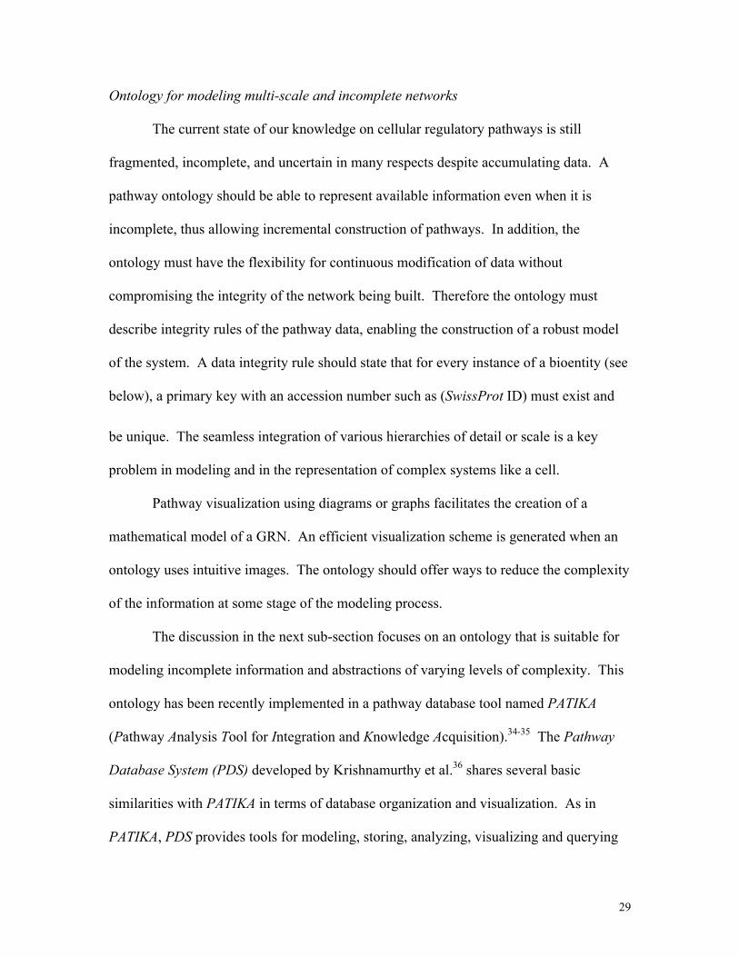
Figure 4. An illustration of the basic features of the PATIKA ontology. States,

transitions, and interactions are represented by circles, rectangles and lines, respectively.

The bioentity “S1” has 3 states (namely, S1, S1' and S1'' ) located in two distinct

subcellular compartments (cytoplasm and nucleus) which are separated by a third

compartment, the nuclear membrane. S1 and S1' are both in the cytoplasm. S1 is

phosphorylated through transition T1 giving rise to a new state, the phosphorylated S1'.

S1' is translocated to the nucleus through transition T2 and becomes S1''. T1 has two

effector states, S2 (inhibitor) and S4 (unspecified effect). T2 has an activator type of

effector (S3) representing, for example, the nuclear pore complex.

32

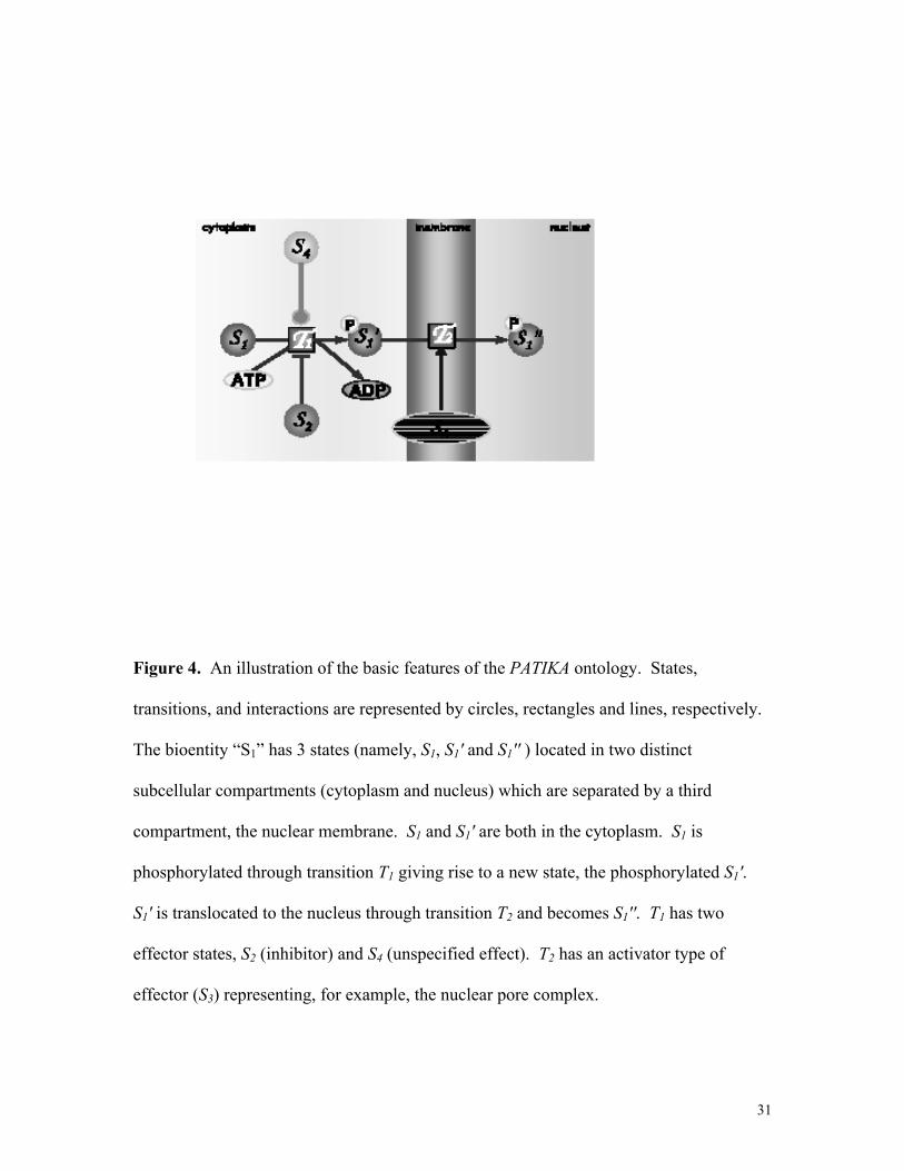
Figure 5. Proposed tree structure used to classify transitions in the PATIKA ontology. If

the nature of a transition can not be defined in the existing ontology, it can be considered

as generic transition to be defined and added in the ontology.

33

Compartments. Transitions also include transport of molecules between cell

compartments. The set of transitions that a state can be involved in is strictly related to its

compartment; accordingly a change in the compartment means a change in the state’s

information context. The state’s compartment is a part of the ontology. As the

compartments and their vicinity are cell-type dependent, compartmental structure can be

modeled as part of the ontology. Cell membranes create an additional complexity since

not only can a molecule be located completely inside the membrane, it may also

communicate with both sides of the membrane as part of the events involved in adjacent

compartments. So membranes are considered as separate compartments in the ontology.

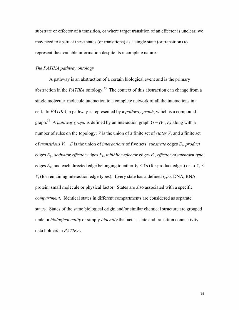
Molecular complexes. In biological systems, molecules often form complexes in

order to perform certain tasks (Fig 6). Each member of a molecular complex can be

considered as a new state of its associated bioentity. The intrinsic specific binding

relations affect the function of a molecular complex. Therefore these binding relations

must be represented in the model ontology. Moreover, members of a molecular complex

may independently participate in different transitions; thus one should be able to address

each member individually (Fig 6). In addition, a molecular complex may contain

members from neighboring compartments (e.g. receptor-ligand complexes).

Abstractions. Various levels of abstractions are employed in the analysis of

complex cellular events. A set of transitions can be described as a single ‘process’ (e.g.

the MAPK pathway), and a set of related processes may be classified under one ‘cellular

mechanism’ (e.g. apoptosis). Some explicit examples of abstractions are shown in Fig 6.

In cases where it is not identified which state among a set of states constitutes the

34

substrate or effector of a transition, or where target transition of an effector is unclear, we

may need to abstract these states (or transitions) as a single state (or transition) to

represent the available information despite its incomplete nature.

The PATIKA pathway ontology

A pathway is an abstraction of a certain biological event and is the primary

abstraction in the PATIKA ontology.35 The context of this abstraction can change from a

single molecule–molecule interaction to a complete network of all the interactions in a

cell. In PATIKA, a pathway is represented by a pathway graph, which is a compound

graph.37 A pathway graph is defined by an interaction graph G = (V , E) along with a

number of rules on the topology; V is the union of a finite set of states Vs and a finite set

of transitions Vt . E is the union of interactions of five sets: substrate edges Es, product

edges Ep, activator effector edges Ea, inhibitor effector edges Ei, effector of unknown type

edges Eu, and each directed edge belonging to either Vt × Vs (for product edges) or to Vs ×

Vt (for remaining interaction edge types). Every state has a defined type: DNA, RNA,

protein, small molecule or physical factor. States are also associated with a specific

compartment. Identical states in different compartments are considered as separate

states. States of the same biological origin and/or similar chemical structure are grouped

under a biological entity or simply bioentity that act as state and transition connectivity

data holders in PATIKA.

35

Figure 6. A pathway containing two abstractions and a molecular complex C1

(composed of three states S1, S2 and S3). Super-state S4 is an example of an abstraction in

which the state S4-P or S4’ may act as an activator of transition T2. S5 leads to the

dissociation of complex C1 acting on either before or after the dissociation of S2.

Therefore S5 may be an activator of either T3 or T4 ; thus, S5 is illustrated as the activator

of super-transition T3-4.

36

Every transition must be affiliated with at least one substrate and one product

edge. It may have an arbitrary number of effectors, a combination of which defines the

exact behavior for the transition. Transitions are classified according to the tree shown in

Fig 5. A transition is not associated with a specific compartment; instead, its

compartment is determined by its interacting states. Different types of molecules (e.g.

protein, DNA and RNA) have distinct user interfaces for easier visual discrimination in

PATIKA. Compartmental information is also modeled. PATIKA also implements

collaborative construction and modification to existing regulatory signaling data on the

database. Therefore PATIKA maintains version numbers as part of the ID of each graph

object. Thus it is possible that while a user is working on a PATIKA graph locally, others

might change the topology and/or properties of states and transitions in the PATIKA

database.

EXTRACTING MODELS FROM PATHWAYS DATABASES

A clear pathway ontology, as discussed in the previous section, will allow

systematic methods for extracting GRN models from the interactions stored in a

pathways database. The specific model would, of course, depend on the particular

biological question being asked. Here, a brief example is given of how a model is

extracted from a network of interactions taken from some of the databases listed in Table

5. The work of Aguda and Tang38 on the G1 checkpoint of the cell cycle is used as an

example. A cell cycle checkpoint is a surveillance mechanism that arrests or slows down

cell cycle progression if something goes wrong, e.g. DNA damage. The significance of

37

elucidating the control mechanism of the G1 checkpoint lies in the observation that many

human cancers are associated with nonfunctional G1 checkpoints.

A qualitative network of the G1-S transition is shown in Fig 7. The network was

generated by integrating information from the published literature, including sequence

analysis of upstream regulatory regions of genes that are targeted by the E2F

transcription factor family. Aguda and Tang38 were interested in finding a minimal

subnetwork that is sufficient to explain the switching behavior of the G1 checkpoint. The

key step towards finding this subnetwork was the hypothesis that there is a core set of

interactions with an intrinsic instability that ultimately generates a switching behavior

(see refs. 38 and 39 for details; network stability analysis is discussed in the next section).

Experimentally, the activity of cyclin E/CDK2 is used as a marker for the entry into the S

phase of the cell cycle. Hence, this minimal set of interactions must include

cyclinE/CDK2.

In the network graph shown in Fig 7, the arrows are interpreted as “activation”

and the hammerheads as “inhibition”. From this qualitative network, a network stability

analysis (discussed in the next section) pointed to a core mechanism involving cyclin

E/CDK2, Cdc25A, p27Kip1 and their interactions. These interactions involve two

coupled positive feedback loops, namely, between the pair (Cdk2/Cyclin E, Cdc25A) and

the pair (Cdk2/Cyclin E, p27). This core mechanism was then used as the basis for a

more detailed mechanistic model. The dynamics of the model was coded into differential

equations and solved in a computer. The computer simulations reproduced the

experimentally observed qualitative behavior of the G1 checkpoint.38

38

A discussion of the mathematical and computational tools already available for

the analysis of GRN models is given in the next section. Most of the models extracted

from pathways databases are expected to be qualitative and incomplete in nature; hence

the discussion focuses on qualitative network structures and how these structures

influence the capacity of the system to exhibit certain dynamical behavior.

39

Figure 7. A qualitative network involving key interactions in the G1-S transition of the

mammalian cell cycle. Solid lines are post-translational modifications or protein-protein

interactions. Dashed arrows are transcriptional steps. Arrows mean “activation”, and

hammerheads mean “inhibition”. GFs = growth factors, cdk = cyclin-dependent kinase,

pRb = retinoblastoma protein, ORC = origin recognition complex.

40

PATHWAY AND DYNAMIC ANALYSIS TOOLS FOR GRNS

Selection of the appropriate network analysis tool depends on the questions being

asked and the scale or size of the network being considered. Questions of robustness of

the entire system against perturbations require more consideration of global network

properties and less of the attributes of individual processes or reactions. Questions

focusing on particular phenomena, such as the switching behavior of a particular set of

genes, may require more attention to the local network details involving these genes.

How the global and local network properties interplay to produce local or system-level

behavior is an important problem that requires multi-scale analysis, both in time and

space. In this section, a brief account is given on global network properties, how large

networks can be analyzed or reduced by identifying recurring network motifs and

extreme pathways, and how topology or network structure alone may already determine a

network’s stability and its capacity to exhibit certain dynamical behavior. The goal of

this section is not to provide a comprehensive review of the aforementioned topics (as

they are quite broad and recent reviews will be cited) but, instead, to point out particular

directions of analysis of a GRN model once it has been constructed.

Global network properties

Considering the very large number of interacting genes, proteins and other

molecules in a living cell, one would first like to ask questions about global features and

properties of the entire network. How connected are the nodes in the network, and what

is the mean path length between any two nodes? Are there clusters of interactions so that

41

one may subdivide the network into modules? How robust is the system to perturbations

– i.e. are there redundant pathways that could take over if a pathway is cut off, so that the

system’s function is still intact? In general, the aim is to identify global network

topological features that affect system function or behavior independent of the details of

the individual nodes or interactions. There had been various attempts at searching for

quantifiable structural features of metabolic networks, signaling networks, and GRNs

(see Ref. 40 for a review). Some basic network descriptors are the degree distribution,

the path length distribution, and the clustering coefficient.

The degree distribution P(k) is the probability that a node is linked to k other

nodes. The P(k) of random networks exhibits a Poisson distribution whereas that of

scale-free networks approximates a power law of the form P(k) ~k-γ. An interesting

suggestion is that most cellular networks approximate a scale-free topology41-42 with an

exponent γ between 2 and 3.43-44 The interpretation of this suggestion is not clear.

The path length distribution of a network tells us how far nodes are from each

other. Scale-free networks are ‘ultra-small’ since they have an average path length of the

order log(log N), where N is the number of nodes. Random networks are ‘small’ because

their mean path length is of the order log N .43-44

The clustering coefficient of a particular node A of a network is defined by C(A)

= 2n(A) / (k(A)(k(A)-1)), where k(A) is the number of neighbors of A, and n(A) is the

number of connections between the neighbors of A.40 The average clustering coefficient

characterizes the tendency of a network to form node clusters, and is a measure of the

network's modularity. The average clustering coefficient of most real networks is larger

42

than that of same-size random networks.45 Cellular networks have a high average

clustering coefficient, which indicates a highly modular structure.46-47

Recurring network motifs

One approach that could simplify the analysis of a large network is to look for

recurring motifs which are subgraphs that are over-represented in the network.48-51 The

motivation is that each motif can be analyzed separately for its intrinsic properties, and

the original network may be reduced to a set of motif interactions. Recent analysis48

show that three-node feed-forward motifs are abundant in transcriptional regulatory

networks and neural networks, while four-node feedback loops are characteristic of

electric circuits, but not of biological networks. Remarkable evolutionary conservation

of motifs52 and convergent evolution toward the same motif types in transcriptional

regulatory networks of diverse species53-54 show that motifs are indeed significant

biologically.

Identifying pathway channels in networks: extreme pathway analysis

Another way of coping with large networks involves breaking down the network

into channels through which distinct processes are carried out. Clarke55 developed a

formalism called ‘Stoichiometric Network Analysis’ and was the first to show that all

steady-state fluxes are found in a convex set called the ‘current cone’; furthermore, he

showed that each cone has a certain number of edge vectors that can be uniquely

determined from the stoichiometric matrix. Clarke referred to the pathways

corresponding to the edge vectors as ‘extreme currents’; alternatively, these are called

43

extreme pathways in this chapter. Recent algorithms for computing extreme pathways

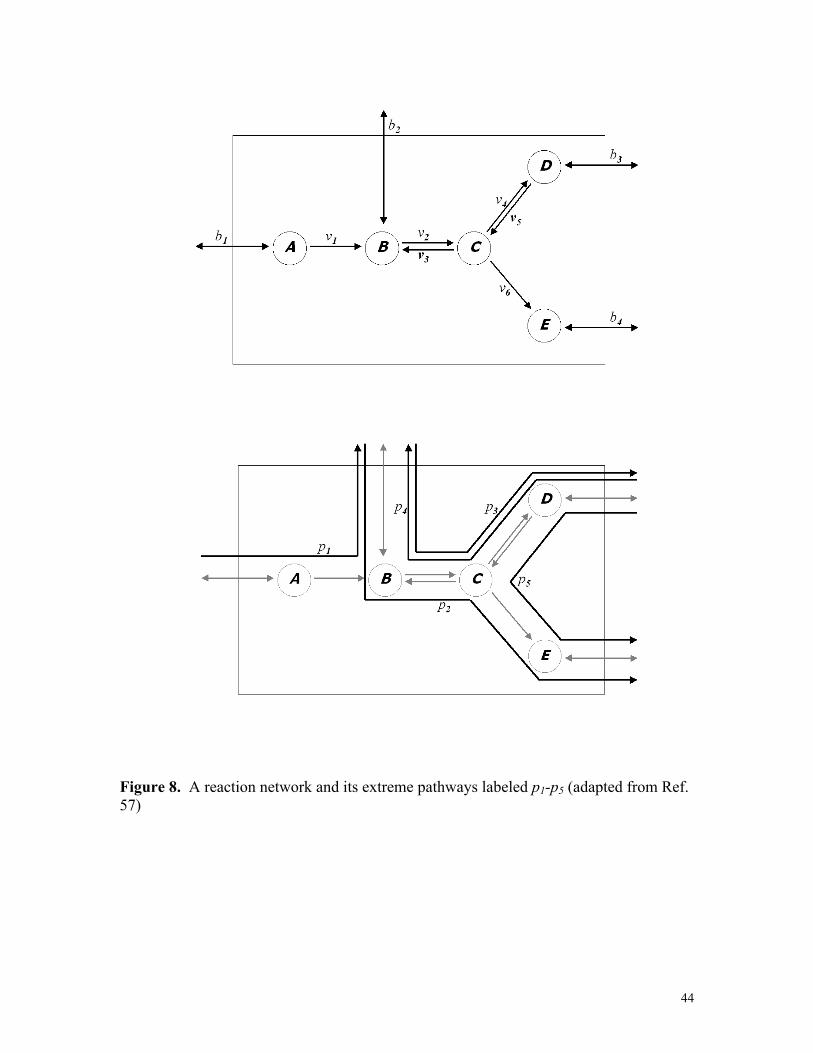
can be found in references 56 and 57. The network shown in Fig 8 serves as an

illustration of the basic ideas of extreme pathway analysis. In the network of Fig 8, there

are six internal fluxes (labeled v1-v6), and four exchange fluxes (the reversible arrows b1-

b4 showing exchange across the rectangular boundary). Except for the two cycling

pathways corresponding to the two reversible reactions (v2-v3 and v4-v5), the five extreme

pathways are shown in the lower panel of Fig 8. Extreme pathway analysis has been

extensively applied to metabolic networks.56-57

Network stability analysis

One of the usual purposes of GRN modeling is to determine the origins of

switching or threshold behaviors. These behaviors are often associated with the stability

properties of the system against perturbations. Would initial perturbations of a species or

a reaction in the network die out or would it reverberate throughout the network? It can

be shown that, at least near steady states, the stability of the network is influenced by the

network structure to a large extent.

More often than not, kinetic or other rate parameters are unknown in GRNs. Only

the qualitative interactions between species are usually known, e.g. “X activates Y” or “V

inhibits W”. As mentioned earlier, one can interpret the meaning of these qualitative

interactions as follows: ∂(dY/dt)/∂X > 0, and ∂(dW/dt)/∂V < 0 , respectively. A

44

Figure 8. A reaction network and its extreme pathways labeled p1-p5 (adapted from Ref. 57)

45

‘qualitative network’ can be defined as a set of nodes (species) and a set of qualitative

interactions (‘activation’ and ‘inhibition’). Note that these qualitative interactions are

none other than the elements of the Jacobian matrix of a linearized system of differential

equations. The state x of a linear dynamical system varies according to the differential

equation

dx / dt = Ax [4]

where A = [aij] is an n × n matrix, and n is the number of species. For the case of a

biochemical network, x is the vector of perturbations from a steady state. This dynamical

system is stable if each solution x(t) approaches zero for t large enough. A weaker

condition is that the dynamical system is semistable, which means that, as t becomes

larger and larger, the solution x(t) could increase, but not at an exponential rate. It is well

known that the dynamical system in equation [4] is stable if and only if all eigenvalues of

A have negative real parts, and it is semistable if and only if all eigenvalues of A have

nonpositive real part. The eigenvalues λ of the matrix A is given by the roots of the

characteristic polynomial:

det(λI-A) = λn + α1λn-1 + α2λ

n-2 +… +α n-1λ + αn = 0 [5]

The coefficients αi are functions of the elements of A and, more importantly, the αi’s are

functions of cycles in the qualitative network graph.58 An example of cycles would be

the three-cycle (a12a23a31) and the one-cycle (aii). The eigenvalues, and therefore the

linear stability of a network, are determined only by cycles in the qualitative network

graph.

Suppose that only the sign pattern of the matrix A is known, i.e., the magnitudes

of aij matrix entries are unknown but their algebraic signs are known. If all matrices that

46

have the same sign pattern as A are stable then A is referred to as sign-stable. If all

matrices that have the same sign pattern as A are semistable then A is sign-semistable.

The notion of sign-semistability has a simple characterization in terms of signs of

the entries of the matrix A (the notion of sign-stability can also be characterized in terms

of signs of the entries of the matrix A, but in a more complicated way59 ). A useful

theorem60 states that A is sign-semistable if and only if three conditions are met: (i) there

is no excitatory one-cycle, (ii) any two-cycle must be negative (i.e. one edge must be

inhibitory and the other excitatory), and (iii) there are no cycles of length three. Note that

since lack of sign-semistability implies lack of sign-stability, the theorem60 on sign-

semistability also gives a set of necessary conditions for sign-stability.

Predicting dynamics and bistability from network structure alone

It will be useful to identify or classify classes of network structures that, from

their structures alone, it is possible to tell whether they have the capacity to exhibit

certain behavior. Given a biochemical reaction network, one can ask the following

question: are there circumstances under which this network would exhibit phenomena

like periodic oscillations and/or bistability? For example, one would want to know the

answer to this question when modeling the cell division cycle and circadian rhythm

where periodic oscillations are required. For mass-action kinetics models, an extensive

theoretical work already exists that answers this type of question for large classes of

reaction networks. One such set of results is the deficiency theory.61-64 The deficiency δ

of a reaction network is a function of the number of objects and linkages in the network

and can be computed easily even if the rate expressions and kinetic parameters are

47

unknown. For reaction networks with δ = 0 it was shown that they do not have the

capacity to exhibit cyclic variation or bistability.63 Feinberg also showed that some

networks with deficiency δ > 0 also do not have the capacity for bistability, if they have

some additional properties.64 These methods are implemented in the software package

called Chemical Reaction Network Toolbox.64-65 Recently, other methods of deciding on

the capacity for bistability of biochemical reaction networks were developed.66-67 The SR

graph method of Craciun and Feinberg67 allows one to draw conclusions on the capacity

of a network to exhibit bistability based on the properties of cycles in the graph.

CONCLUDING REMARKS

With a well defined pathway ontology, one could envisage a computer program

that automates the analysis of complex gene regulatory networks and the extraction or

building of GRN models; these models can then be analyzed by computer simulation and

other mathematical methods. An investigator would most likely start with a short list of

genes or even a short list of specific cellular processes (from which a gene list could be

derived using existing gene annotations such as GeneOntology). By scouring databases,

the computer program would then try to establish pathways among the initial set of

genes; this step will increase the number of genes in the network and also include

proteins and other molecules regulating the pathways. At this point, the GRN is a static

graph, perhaps a qualitative network containing some information about how the nodes

affect each other. The computer program can now use network analysis tools to study the

48

topology of the GRN and to identify stabilizing or destabilizing cycles, extreme

pathways, or even try to reduce the size of the network without removing the capacity for

certain behaviors of interest. Databases (including the published literature) containing

experimental information will have to be consulted to validate the significance or strength

of contribution of the pathways and cycles present in the reduced model. The rate

expressions and associated kinetic parameters of the individual steps in the model are

then supplied to a solver of the dynamical equations to simulate the temporal evolution of

the model system. Predictions of the model will have to be compared with experimental

data, and the process of model refinement and experimental validation could be iterated.

As the work of Ozbudak et al.3 and Vilar, Guet and Leibler4 on the lac operon

demonstrated, abstract kinetic models with a few variables are sometimes sufficient to

capture the essential behavior of the system, e.g. the bistable switch in the lac operon. It

may seem that there is some arbitrariness in how these simple lac operon models3-4 were

generated, since they seem to look very different and the dynamical variables are not the

same. However, both models preserve the common property of having a positive

feedback loop. The presence of such a loop has long been known, in dynamical systems

theory, to give a system the ability to generate bistability given the right parameters. As

the work of Ozbudak et al.3 showed, a low-dimensional abstract model can indeed be

predictive. In the future, the process of extracting an abstract model from a complex

GRN may well be carried out systematically. The key will be the application of the

mathematical fields of nonlinear dynamics and reaction network analysis. As mentioned

in this chapter, possible behavior of networks may already be predicted from their

qualitative network structures regardless of the values of rate parameters. The

49

development of a pathway ontology that can interface with network structure analysis

tools will be crucial for the integration and use of the huge amounts of data stored in

databases.

Significant advances towards understanding gene networks are coming from

recent work on synthetic gene networks (see ref. 68 for a recent review); the goal here is

the construction and engineering control of genetic circuits built from well understood

building blocks of small gene modules. What is being learned from these man-made

gene networks will be very useful in future analysis of the very complex GRN repertoire

of a living cell.

50

REFERENCES

1. P. Wong, S. Gladney, and J. D. Keasling, Biotechnol. Prog., 13, 132 (1997).

Mathematical Model of the Lac Operon: Inducer Exclusion, Catabolite Repression, and

Diauxic Growth on Glucose and Lactose.

2. N. Yildirim and M. C. Mackey, Biophysical Journal, 84, 2841 (2003). Feedback

Regulation in the Lactose Operon: A Mathematical Modeling Study and Comparison

with Experimental Data.

3. E. M. Ozbudak, M. Thattai, H. N. Lim, B. I. Shraiman, and A. van Oudenaarden,

Nature, 427, 737 (2004). Multistability in the Lactose Utilization Network of

Escherichia coli.

4. J. M. G. Vilar, C C. Guet, and S. Leibler, J. Cell Biology, 161, 471 (2003). Modeling

Network Dynamics: The Lac Operon, A Case Study.

5. F. Jacob, D. Perrin, C. Sanchez, and J. Monod, Compt. Rendu. Acad. Sci., 245, 1727

(1960). L'operon: Groupe de Genes a l'Expression Coordonne par un Operateur.

6. J. J. Tyson and H. G. Othmer, in Progress in Biophysics, R. Rosen, Ed., Academic

Press, New York, 5, 1 (1978). The Dynamics of Feedback Control Circuits in

Biochemical Pathways.

51

7. D. M. Wolf and F. H. Eeckman, J. Theor. Biol., 195, 167 (1998). On the Relationship

between Genomic Regulatory Element Organization and Gene Regulatory Dynamics.

8. J. J. Tyson, K. C. Chen, and B. Novak, Curr. Opin. Cell Biol., 15, 221 (2003).

Sniffers, Buzzers, Toggles and Blinkers: Dynamics of Regulatory and Signaling

Pathways in the Cell.

9. H. de Jong, J. Comput. Biol., 9, 67 (2002). Modeling and Simulation of Genetic

Regulatory Systems: A Literature Review.

10. N. Friedman, Science, 303, 799 (2004). Inferring Cellular Networks Using

Probabilistic Graphical Models.

11. E. P. van Someren, L. F. A. Wessels, E. Backer, and M. J. T. Reinders,

Pharmacogenomics, 3, 507 (2002). Genetic Network Modeling.

12. J. Stark, D. Brewer, M. Barenco, D. Tomescu, R. Callard, and M. Hubank, Biochem.

Soc. Trans., 31, 1519 (2003). Reconstructing Gene Networks: What are the Limits?

13. J. Stark, R. Callard, and M. Hubank, Trends Biotech., 21, 290 (2003). From the Top

Down: Towards a Predictive Biology of Signaling Networks.

52

14. P. D’haeseleer, S. Liang, and R. Somogyi, Bioinformatics, 16, 707 (2000). Genetic

Network Inference: From Co-expression Clustering to Reverse Engineering.

15. M. B. Eisen, P. T. Spellman, P. O. Brown, and D. Botstein, Proc. Natl. Acad. Sci.

USA, 95, 14863 (1998). Cluster Analysis and Display of Genome-Wide Expression

Patterns.

16. J. Wang, O. Myklebost, and E. Hovig, Bioinformatics, 19, 2210 (2003). MGraph:

Graphical Models for Microarray Data Analysis.

17. D. Husmeier, Biochem. Soc. Trans., 31, 1516 (2003). Reverse Engineering of

Genetic Networks with Bayesian Networks.

18. D. Husmeier, Bioinformatics, 19, 2271 (2003b). Sensitivity and Specificity of

Inferring Genetic Regulatory Interactions from Microarray Experiments with Dynamic

Bayesian Networks.

19. N. Friedman, M. Linial, I. Nachman, and D. Pe’er, J. Comput. Biol., 7, 601 (2000).

Using Bayesian networks to Analyze Expression Data.

20. D. Pe’er, A. Regev, G. Elidan, and N. Friedman, Bioinformatics, 17, S215 (2001).

Inferring Subnetworks from Perturbed Expression Profiles.

53

21. A. J. Hartemink, D. K. Gifford, T. S. Jaakkola, and R. A. Young, Pac. Symp.

Biocomput., 6, 422 (2001). Using Graphical Models and Genomic Expression Data to

Statistically Validate Models of Genetic Regulatory Networks.

22. D. E. Zak, F. J. Doyle, and J. S. Schwaber, Proceedings of the Third International

Conference on Systems Biology, Karolinska Institute, Sweden, pp. 236-237 (2002). Local

Identifiability: When can Genetic Networks be Identified from Microarray Data?

23. A. de la Fuente, P. Brazhnik, and P. Mendes, Trends Genet., 18, 395 (2002). Linking

the Genes: Inferring Quantitative Gene Networks from Microarray Data.

24. B. N. Kholodenko, A. Kiyatkin, F. J. Bruggeman, E. Sontag, H. V. Westerhoff, and

J. B. Hoek, Proc. Natl. Acad. Sci. USA, 99, 12841 (2002). Untangling Wires: A Strategy

to Trace Functional Interactions in Signaling and Gene Networks.

25. T. S. Gardner, D. di Bernardo, D. Lorenz, and J. J. Collins, Science, 301, 102 (2003).

Inferring Genetic Networks and Identifying Compound Mode of Action via Expression

Profiling.

26. M. Y. Galperin, Nucleic Acids Res., 32, D3 (2004). The Molecular Biology Database

Collection: 2004 update.

54

27. C. Lemer, E. Antezana, F. Couche, F. Fays, X. Santolaria, R. Janky, Y. Deville, J

Richelle, and S.J. Wodak, Nucleic Acids Res., 32, D443 (2004). The aMAZE

LightBench: A Web Interface to a Relational Database of Cellular Processes.

28. T. R. Gruber. Knowledge Acquisition, 5, 199 (1993). A Translation Approach to

Portable Ontologies.

29. P. Mendes, Trends Biochem. Sci., 22, 361 (1997). Biochemistry by Numbers:

Simulation of Biochemical Pathways with Gepasi 3.

30. B. M. Slepchenko, J. C. Schaff, I. Macara, and L. M. Loew, Trends Cell Biol., 13,

570 (2003). Quantitative Cell Biology with the Virtual Cell.

31. M. Tomita, K. Hashimoto, K. Takahashi, T. Shimizu, Y. Matsuzaki, F. Miyoshi, K.

Saito, S. Tanida, K. Yugi, J. C. Venter, and C. A. Hutchison, Bioinformatics., 15, 72

(1999). E-CELL: Software Environment for Whole-Cell Simulation.

32. K. Takahashi, N. Ishikawa, Y. Sadamoto, H. Sasamoto, S. Ohta, A. Shiozawa, F.

Miyoshi, Y. Naito, Y. Nakayama, and M. Tomita, Bioinformatics., 19, 1727 (2003). E-

Cell 2: Multi-Platform E-Cell Simulation System.

33. P. Dhar, T.C. Meng, S. Somani, L. Ye, A. Sairam, M. Chitre, Z. Hao, and K.

Sakharkar, Bioinformatics., 20, 1319 (2004). Cellware: A Multi-Algorithmic Software

for Computational Systems Biology.

55

34. E. Demir, O. Babur, U. Dogrusoz, A. Gursoy, G. Nisanci, R. Cetin-Atalay, and M.

Ozturk, Bioinformatics., 18, 996 (2002). PATIKA: An Integrated Visual Environment for

Collaborative Construction and Analysis of Cellular Pathways.

35. E. Demir, O. Babur, U. Dogrusoz, A. Gursoy, A. Ayaz, G. Gulesir, G. Nisanci, and

R. Cetin-Atalay, Bioinformatics., 20, 349 (2004). An Ontology for Collaborative

Construction and Analysis of Cellular Pathways.

36. L. Krishnamurthy, J. Nadeau, G. Ozsoyoglu, M. Ozsoyoglu, G. Schaeffer, M. Tasan,

and W. Xu, Bioinformatics., 22, 930, (2003). Pathways Database System: An Integrated

System for Biological Pathways.

37. K. Fukuda and T. Takagi, Bioinformatics, 17, 829 (2001). Knowledge

Representation of Signal Transduction Pathways.

38. B. D. Aguda and Y. Tang, Cell Proliferation, 32, 321 (1999). The Kinetic Origins of

the Restriction Point in the Mammalian Cell Cycle.

39. B. D. Aguda, Oncogene 18, 2846 (1999). Instabilities in Phosphorylation

Dephosphorylation Cascades and Cell Cycle Checkpoints.

40. A.-L. Barabasi and Z. N. Oltvai, Nat. Rev. Genet., 5, 101 (2004). Network Biology:

Understanding the Cell's Functional Organization.

56

41. H. Jeong, B. Tombor, R. Albert, Z. N. Oltvai, and A.-L. Barabasi, Nature, 407, 651

(2000). The Large-Scale Organization of Metabolic Networks.

42. A. Wagner and D. A. Fell, Proc. R. Soc. Lond. B, 268, 1803 (2001). The Small

World Inside Metabolic Networks.

43. F. Chung and L. Lu, Proc. Natl. Acad. Sci. USA, 99, 15879 (2002). The Average

Distances in Random Graphs with Given Expected Degrees.

44. R. Cohen and S. Havlin, Phys. Rev. Lett., 90, 058701 (2003). Scale-Free Networks

are Ultra Small.

45. D. J. Watts and S. H. Strogatz, Nature, 393, 440 (1998). Collective Dynamics of

‘Small-World’ Networks.

46. A. Wagner, Mol. Biol. Evol., 18, 1283 (2001). The Yeast Protein Interaction Network

Evolves Rapidly and Contains Few Redundant Duplicate Genes.

47. S. Wuchty, Mol. Biol. Evol., 18, 1694 (2001). Scale-Free Behaviour in Protein

Domain Networks.

48. R. Milo, S. S. Shen-Orr, S. Itzkovitz, N. Kashtan, D. Chklovskii, and U. Alon,

Science, 298, 824 (2002). Network Motifs: Simple Building Blocks of Complex

Networks.

57

49. S. Itzkovitz, R. Milo, N. Kashtan, G. Ziv, and U. Alon, Phys. Rev. E Stat. Nonlin.

Soft Matter Phys., 68, 026127 (2003). Subgraphs in Random Networks.

50. E. Yeger-Lotem, S. Sattath, N. Kashtan, S. Itzkovitz, R. Milo, R. Y. Pinter, and U.

Alon, Proc. Natl. Acad. Sci. USA, 101, 5934 (2004). Network Motifs in Integrated

Cellular Networks of Transcription-Regulation and Protein-Protein Interaction.

51. J. Ihmels, G. Friedlander, S. Bergmann, O. Sarig, Y. Ziv, and N. Barkai, Nature

Genet., 31, 370 (2002). Revealing Modular Organization in the Yeast Transcriptional

Network.

52. S. Wuchty, Z. N. Oltvai, and A.-L. Barabasi, Nature Genet., 35,176 (2003).

Evolutionary Conservation of Motif Constituents within the Yeast Protein Interaction

Network.

53. G. C. Conant and A. Wagner, Nature Genet., 34, 264 (2003). A Convergent

Evolution of Gene Circuits.

54. V. F. Hinman, A. T. Nguyen, R. A. Cameron, E. H. Davidson, Proc. Natl. Acad. Sci.

USA, 100(23), 13356 (2003). Developmental Gene Regulatory Network Architecture

Across 500 Million Years of Echinoderm Evolution.

58

55. B. L. Clarke, Adv. Chem. Phys., 43, 1 (1980). Stability of Complex Reaction

Networks.

56. J. A. Papin, N. D. Price, and B. Ø. Palsson, Genome Res., 12, 1889 (2000). Extreme

Pathway Lengths and Reaction Participation in Genome-Scale Metabolic Networks.

57. C. Schilling, D. Letscher, and B. Ø. Palsson, J. Theor. Biol., 203, 229 (2000). Theory

for the Systemic Definition of Metabolic Pathways and their use in Interpreting

Metabolic Function from a Pathway-Oriented Perspective.

58. C. J. Puccia and R. Levins, Qualitative Modeling of Complex Systems: An

Introduction to Loop Analysis and Time Averaging. Harvard University Press,

Cambridge, Mass., 1985.

59. V. Klee, in Applications of Combinatorics and Graph Theory to the Biological and

Social Sciences, F. Roberts, Ed., IMA Volumes in Mathematics and Its Applications,

Springer, New York, 17, 1989, pp. 203-219. Sign-Patterns and Stability.

60. J. Quirk and R. Ruppert, Rev. Economic Studies, 32, 311 (1965). Qualitative

Economics and the Stability of Equilibrium.

59

61. M. Feinberg, Arch. Rational Mech. Anal., 49, 187 (1972). Complex Balancing in

General Kinetic Systems.

62. F. Horn, R. Jackson, Arch. Rational Mech. Anal., 47, 81 (1972). General Mass

Action Kinetics.

63. M. Feinberg, Lectures on Chemical Reaction Networks, written version of lectures

given at the Mathematical Research Center, University of Wisconsin, Madison.

Mathematical Research Center, University of Wisconsin, 1979.

64. M. Feinberg, Arch. Rational Mech. Anal., 132, 311, (1995). The Existence and

Uniqueness of Steady States for a Class of Chemical Reaction Networks.

65. M. Feinberg, Chemical Reaction Network Toolbox, Version 1.02 (1995), and Version

1.1 (1999, with P. Ellison) available for download at http:// www.che.eng.ohio-

state.edu/~feinberg/crnt

66. G. Craciun and M. Feinberg, SIAM J. Appl. Math., in press (2004). Multiple

Equilibria in Complex Chemical Reaction Networks: The Injectivity Property.

67. G. Craciun and M. Feinberg, Mathematical Biosciences Institute Technical Report,

22 (2004). Multiple Equilibria in Complex Chemical Reaction Networks: The SR Graph.

60

68. R. Weiss, S. Basu, S. Hooshangi, A. Kalmbach, D. Karig, R. Mehreja, and I.

Netravali, Natural Computing, 2, 47 (2003). Genetic Circuit Building Blocks for Cellular

Computation, Communications, and Signal Processing.