Darshan Institute of Engineering and Technology 180702 - Parallel Processing Computer Engineering Chapter - 2 Parallel Programming Platforms Ishan Rajani 1 1) What is implicit parallelism? Explain pipelining and superscalar execution in parallel processing with suitable example. [Oct. 13(7 marks), June 12(7 marks)] Current processors use resources in multiple functional units and execute multiple instructions in the same cycle. The precise manner in which these instructions are selected and executed provides impressive diversity in architectures. In computer science, implicit parallelism is a characteristic of a programming language that allows a compiler or interpreter to automatically exploit the parallelism. Implicit Parallelism is a parallel programming model which aims to take advantage of the parallelism already inherent in the structure of a programming language. This is opposed to Explicit Parallelism which involves user-specified parallel instructions. A programmer that writes implicitly parallel code does not need to worry about task division or process communication, focusing instead in the problem that his or her program is intended to solve. Languages with implicit parallelism reduce the control that the programmer has over the parallel execution of the program. Though Implicit Parallelism may at first seem a great deal like Automatic Parallelism, it actually differs significantly because language structures can be built in such a way to restrict coding practices. Mechanisms used by various processors for supporting multiple instruction execution: Pipelining: Processors use the concept of pipeline to improve execution rate. An instruction pipeline is a technique used in the design of computer to increase their instruction throughput (the number of instructions that can be executed in a unit of time). By overlapping various stages in instruction execution (instruction fetch, decode, execute, memory access, write back to registers), pipelining enables faster execution. Speed increases as the number of stages of pipeline increased. Superscalar Execution: A processor with more than one pipelines and the ability to simultaneously issue multiple instructions, is sometimes referred to as super-pipelined processor. The ability of a processor to issue multiple instructions in the same cycle is referred to as superscalar execution.

Welcome message from author
This document is posted to help you gain knowledge. Please leave a comment to let me know what you think about it! Share it to your friends and learn new things together.
Transcript
Darshan Institute of Engineering and Technology 180702 - Parallel Processing
Computer Engineering Chapter - 2 Parallel Programming Platforms
Ishan Rajani 1
1) What is implicit parallelism? Explain pipelining and superscalar execution in parallel processing with
suitable example. [Oct. 13(7 marks), June 12(7 marks)]
Current processors use resources in multiple functional units and execute multiple instructions in the
same cycle. The precise manner in which these instructions are selected and executed provides
impressive diversity in architectures.
In computer science, implicit parallelism is a characteristic of a programming language that allows a
compiler or interpreter to automatically exploit the parallelism.
Implicit Parallelism is a parallel programming model which aims to take advantage of the parallelism
already inherent in the structure of a programming language.
This is opposed to Explicit Parallelism which involves user-specified parallel instructions.
A programmer that writes implicitly parallel code does not need to worry about task division or
process communication, focusing instead in the problem that his or her program is intended to solve.
Languages with implicit parallelism reduce the control that the programmer has over the parallel
execution of the program.
Though Implicit Parallelism may at first seem a great deal like Automatic Parallelism, it actually differs
significantly because language structures can be built in such a way to restrict coding practices.
Mechanisms used by various processors for supporting multiple instruction execution:
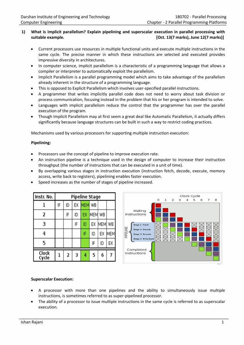
Pipelining:
Processors use the concept of pipeline to improve execution rate.
An instruction pipeline is a technique used in the design of computer to increase their instruction
throughput (the number of instructions that can be executed in a unit of time).
By overlapping various stages in instruction execution (instruction fetch, decode, execute, memory
access, write back to registers), pipelining enables faster execution.
Speed increases as the number of stages of pipeline increased.
Superscalar Execution:
A processor with more than one pipelines and the ability to simultaneously issue multiple
instructions, is sometimes referred to as super-pipelined processor.
The ability of a processor to issue multiple instructions in the same cycle is referred to as superscalar
execution.
Darshan Institute of Engineering and Technology 180702 - Parallel Processing
Computer Engineering Chapter - 2 Parallel Programming Platforms
Ishan Rajani 2
It allows two issues per clock cycle; it is also referred to as two-way superscalar or dual issue
execution.
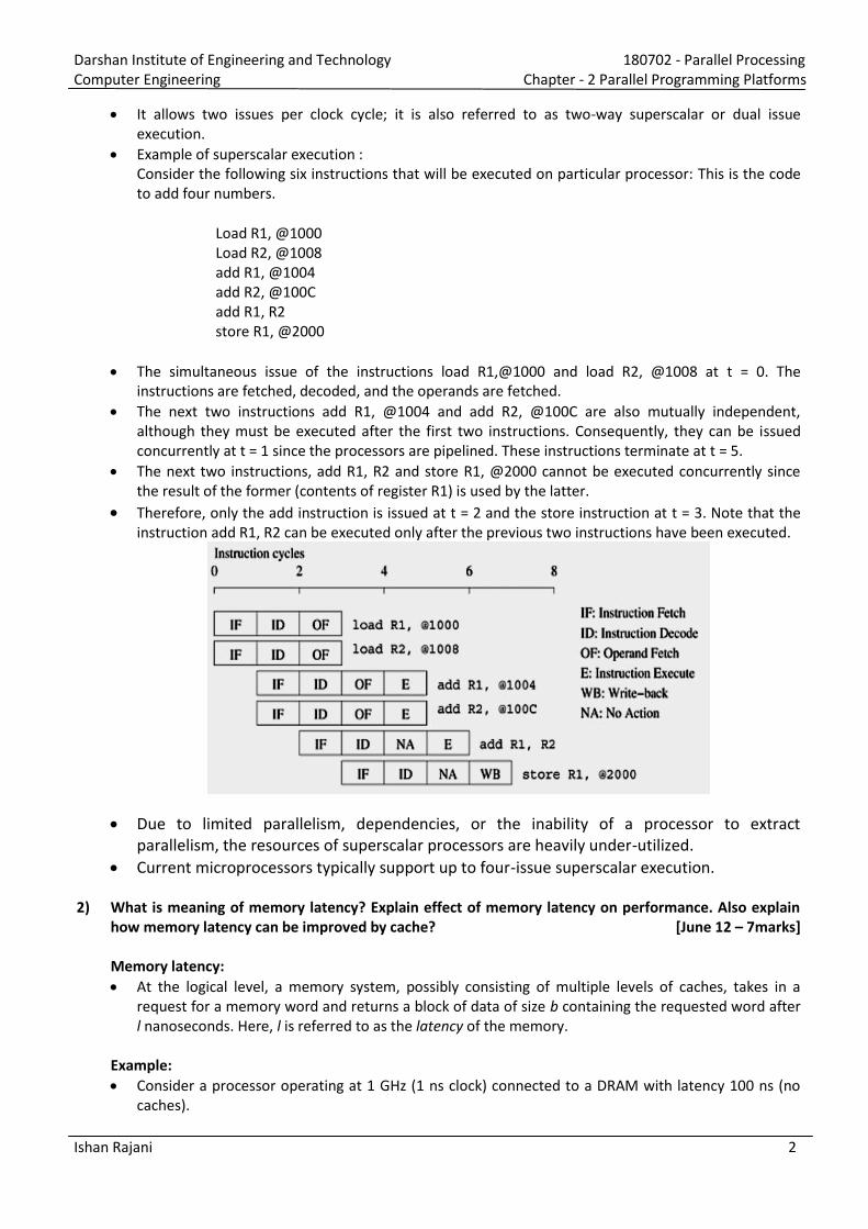
Example of superscalar execution :
Consider the following six instructions that will be executed on particular processor: This is the code
to add four numbers.
Load R1, @1000
Load R2, @1008
add R1, @1004
add R2, @100C
add R1, R2
store R1, @2000
The simultaneous issue of the instructions load R1,@1000 and load R2, @1008 at t = 0. The
instructions are fetched, decoded, and the operands are fetched.
The next two instructions add R1, @1004 and add R2, @100C are also mutually independent,
although they must be executed after the first two instructions. Consequently, they can be issued
concurrently at t = 1 since the processors are pipelined. These instructions terminate at t = 5.
The next two instructions, add R1, R2 and store R1, @2000 cannot be executed concurrently since
the result of the former (contents of register R1) is used by the latter.
Therefore, only the add instruction is issued at t = 2 and the store instruction at t = 3. Note that the
instruction add R1, R2 can be executed only after the previous two instructions have been executed.
Due to limited parallelism, dependencies, or the inability of a processor to extract
parallelism, the resources of superscalar processors are heavily under-utilized.
Current microprocessors typically support up to four-issue superscalar execution.
2) What is meaning of memory latency? Explain effect of memory latency on performance. Also explain
how memory latency can be improved by cache? [June 12 – 7marks]
Memory latency:
At the logical level, a memory system, possibly consisting of multiple levels of caches, takes in a
request for a memory word and returns a block of data of size b containing the requested word after
l nanoseconds. Here, l is referred to as the latency of the memory.
Example:
Consider a processor operating at 1 GHz (1 ns clock) connected to a DRAM with latency 100 ns (no
caches).
Darshan Institute of Engineering and Technology 180702 - Parallel Processing
Computer Engineering Chapter - 2 Parallel Programming Platforms
Ishan Rajani 3
Assume that the processor has two multiply-add units and is capable of executing four instructions in
each cycle of 1 ns. The peak processor rating is therefore 4 GFLOPS.
Since the memory latency is equal to 100 cycles and block size is one word, every time a memory
request is made, the processor must wait 100 cycles before it can process the data.
Consider the program of computing the dot-product of two vectors.
A dot-product computation performs one multiply-add on a single pair of vector elements, i.e., each
floating point operation requires one data fetch.
So the peak speed of this computation is limited to one floating point operation at every 100 ns, or a
speed of 10 MFLOPS which is very low than peek processor rating.
Solution:
Handling the mismatch in processor and DRAM speeds has motivated a number of architectural
innovations in memory system design.
One such innovation addresses the speed mismatch by placing a smaller and faster memory between
the processor and the DRAM. This memory, referred to as the cache, acts as low-latency high-
bandwidth storage.
The data needed by the processor is first fetched into the cache.
All subsequent accesses to data items residing in the cache are serviced by the cache.
Thus, in principle, if a piece of data is repeatedly used, the effective latency of this memory system
can be reduced by the cache.
In our above example of 1 GHz processor with 100 ns latency DRAM if we introduce a cache of size 32
KB with a latency of 1 ns or one cycle.
This corresponds to a peak computation rate of 303 MFLOPS approximately, although it is still less
than 10% of the peak processor performance.
We can see in this example that by placing a small cache memory, we are able to improve processor
utilization.
3) How do you hide memory latency by using prefetching and multithreading? OR
Explain alternate approaches for hiding memory latency. [Oct. 12 - 3 marks]
Multithreading:
A thread is a single stream of control in the flow of a program. Or Thread is a part of sequential flow
of program.
For Example we open multiple browsers and access different pages in each browser, thus while we
are waiting for one page to load, we could be reading others.
Consider the following code segment for multiplying an n x n matrix a a e tor to get e tor .
for(i=0;i<n;i++)
c[i] = dot_product(get_row(a, i), b);
It computes each element of c as the dot product of the corresponding row of a with the vector b.
Notice that each dot-product is independent of the other, and therefore represents a concurrent unit
of execution.
We can safely rewrite the above code segment as:
for(i=0;i<n;i++)
c[i] = create_thread(dot_product, get_row(a, i), b);
Difference between the two code segments is that we have explicitly specified each instance of the
dot-product computation as being a thread.
Now, consider the execution of each instance of the function dot_product. The first instance of this
Darshan Institute of Engineering and Technology 180702 - Parallel Processing
Computer Engineering Chapter - 2 Parallel Programming Platforms
Ishan Rajani 4
function accesses a pair of vector elements and waits for them. In the meantime, the second instance
of this function can access two other vector elements in the next cycle, and so on.
In this way, in every clock cycle, we can perform a computation.
Prefetching :
In a typical program, a data item is loaded and used by a processor in a small time window. If the load
results in a cache miss, then the use stalls.
A simple solution to this problem is to advance the load operation so that even if there is a cache
miss, the data is likely to have arrived by the time it is used.
It is a process to advance the load operation so that even if there is a cache miss, the data is likely to
have arrived by the time it is used.
In advancing the loads, we are trying to identify independent threads of execution that have no
resource dependency (i.e., use the same registers) with respect to other threads.
Co sider the pro le of addi g t o e tors a a d usi g a si gle for loop. I the first iteratio of the loop, the processor requests a[0] and b[0]. Since these are not in the cache, the processor must
pay the memory latency. While these requests are being serviced, the processor also requests a[1]
and b[1].
Assuming that each request is generated in one cycle (1 ns) and memory requests are satisfied in 100
ns, after 100 such requests the first set of data items is returned by the memory system.
Subsequently, one pair of vector components will be returned every cycle.
In this way, in each subsequent cycle, one addition can be performed and processor cycles are not
wasted.
4) Explain message passing and shared-address-space computers with neat sketches. Also state the
differences between these two computers. [June 13(7 marks)]
The "shared-address-space" view of a parallel platform supports a common data space that is
accessible to all processors.
Shared-address-space platforms supporting SPMD programming are also referred to as
multiprocessors.
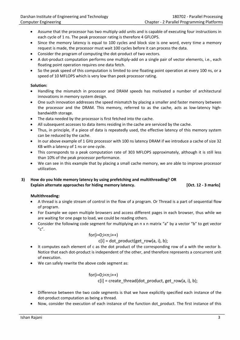
Memory in shared-address-space platforms can be local or global.
If the time taken by a processor to access any memory word in the system (global or local) is
identical, the platform is classified as a uniform memory access (UMA) multicomputer. On the other
hand, if the time taken to access certain memory words is longer than others, the platform is called a
non-uniform memory access (NUMA) multicomputer.
If accessing local memory is cheaper than accessing global memory, algorithms must build locality
and structure data and computation accordingly.
Figures (a) and (b) illustrate UMA platforms, whereas Figure (c) illustrates a NUMA platform.
Here, in figure (b) it is faster to access a memory word in cache than a location in memory. However,
Darshan Institute of Engineering and Technology 180702 - Parallel Processing
Computer Engineering Chapter - 2 Parallel Programming Platforms
Ishan Rajani 5
still classify this as a UMA architecture. The reason for this is that all current microprocessors have
cache hierarchies.
Consequently, even a uniprocessor would not be termed UMA if cache access times are considered.
Read/write interactions are, however, harder to program than the read-only interactions, as these
operations require mutual exclusion for concurrent accesses. Shared-address-space programming
paradigms such as threads and directives therefore support synchronization using locks and related
mechanisms.
Supporting a shared-address-space in this context involves two major tasks:
Providing an address translation mechanism that locates a memory word in the system, and
Ensuring that concurrent operations on multiple copies of the same memory word have well-defined
semantics.
The term shared-memory computer is historically used for architectures, in which the memory is
physically shared among various processors, i.e., each processor has equal access to any memory
segment. This is identical to the UMA model.
This is in contrast to a distributed-memory computer, in which different segments of the memory are
physically associated with different processing elements.
A distributed-memory shared-address-space computer is identical to a NUMA machine.
5) Write a short note on Message Passing Platforms. [Oct. 12(7 marks)]
The logical machine view of a message-passing platform consists of p processing nodes, each with its
own exclusive address space.
Each of these processing nodes can either be single processors or a shared-address-space
multiprocessor.
Interactions between processes running on different nodes must be accomplished using messages,
hence the name message passing.
This exchange of messages is used to transfer data, work, and to synchronize actions among the
processes.
In its most general form, message-passing paradigms support execution of a different program on
each of the p nodes.
Since interactions are accomplished by sending and receiving messages, the basic operations in this
programming paradigm are send and receive.
In addition, since the send and receive operations must specify target addresses; there must be a
mechanism to assign a unique identification or ID to each of the multiple processes executing a
parallel program.
This ID is typically made available to the progra usi g a fu tio su h as hoa i , hi h retur s to a calling process its ID.
There is one other function that is typically needed to complete the basic set of message-passing
operations – u pro s , hi h spe ifies the u er of pro esses parti ipating in the ensemble.
It is easy to emulate a message-passing architecture containing p nodes on a shared-address-space
computer with an identical number of nodes.
However, emulating a shared-address-space architecture on a message-passing computer is costly,
since accessing another node's memory requires sending and receiving messages.
Darshan Institute of Engineering and Technology 180702 - Parallel Processing
Computer Engineering Chapter - 2 Parallel Programming Platforms
Ishan Rajani 6
6) Enlist and explain the various forms of PRAM in brief. [Oct. 13(7 marks), Oct. 12(4 marks)]
Physical Organization of Parallel computer consists of processors called Random Access
Machine, or RAM and a global memory of unbounded size that is uniformly accessible to all
processors.
All processors access the same address space. Processors share a common clock but may
execute different instructions in each cycle. This ideal model is also referred to as a parallel
random access machine (PRAM). Since PRAMs allow concurrent access to various memory
locations, depending on how simultaneous memory accesses are handled, PRAMs can be
divided into four subclasses.
Exclusive-read, exclusive-write (EREW) PRAM. In this class, access to a memory location is
exclusive. No concurrent read or write operations are allowed. This is the weakest PRAM model,
affording minimum concurrency in memory access.
Concurrent-read, exclusive-write (CREW) PRAM. In this class, multiple read accesses to a
memory location are allowed. However, multiple write accesses to a memory location are
serialized.
Exclusive-read, concurrent-write (ERCW) PRAM. Multiple write accesses are allowed to a
memory location, but multiple read accesses are serialized.
Concurrent-read, concurrent-write (CRCW) PRAM. This class allows multiple read and write
accesses to a common memory location. This is the most powerful PRAM model.
Allowing concurrent read access does not create any semantic discrepancies in the program.
However, concurrent write access to a memory location requires arbitration. Several
protocols are used to resolve concurrent writes. The most frequently used protocols are as
follows:
Common, in which the concurrent write is allowed if all the values that the processors are
attempting to write are identical.
Arbitrary, in which an arbitrary processor is allowed to proceed with the write operation and
the rest fail.
Priority, in which all processors are organized into a predefined prioritized list, and the
processor with the highest priority succeeds and the rest fail.
Sum, in which the sum of all the quantities is written (the sum-based write conflict resolution
model can be extended to any associative operator defined on the quantities being written).
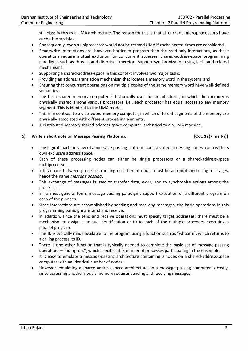
7) Explain multistage network topology. [Oct. 13(7 marks)]
Multistage Networks :
An intermediate class of networks called multistage interconnection networks lies between
these two extremes.
The general schematic of a multistage network consisting of p processing nodes and b
memory banks is shown in Figure.
Darshan Institute of Engineering and Technology 180702 - Parallel Processing
Computer Engineering Chapter - 2 Parallel Programming Platforms
Ishan Rajani 7
Each stage of this network consists of an interconnection pattern that connects p inputs and
p outputs usi g o ega et ork; a li k e ists et ee i put i and output j if the
following is true:
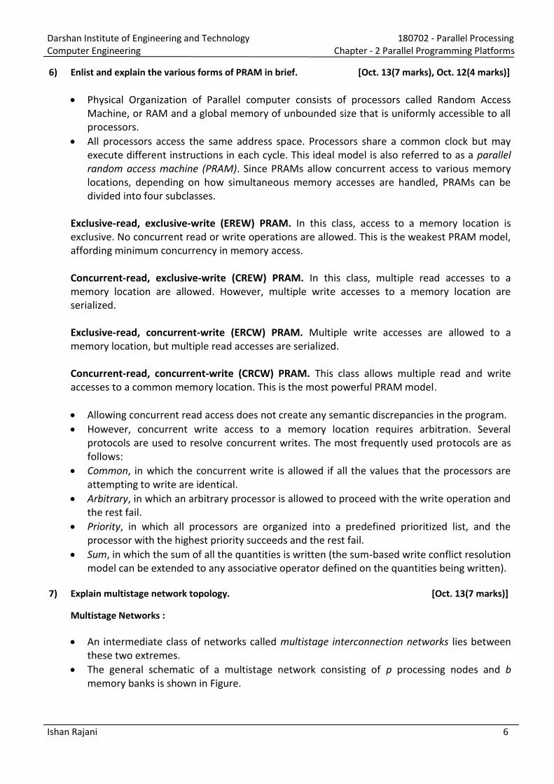
Equation represents a left-rotation operation on the binary representation of i to obtain j.
This interconnection pattern is called a perfect shuffle.
Figure shows a perfect shuffle interconnection pattern for eight inputs and outputs.
The inputs are sent straight through to the outputs, as shown in Figure (a). This is called the
pass-through connection. In the other mode, the inputs to the switching node are crossed
over and then sent out, as shown in Figure (b). This is called the cross-over connection.
It is more scalable than the bus in terms of performance and more scalable than the crossbar
in terms of cost.
Darshan Institute of Engineering and Technology 180702 - Parallel Processing
Computer Engineering Chapter - 2 Parallel Programming Platforms
Ishan Rajani 8
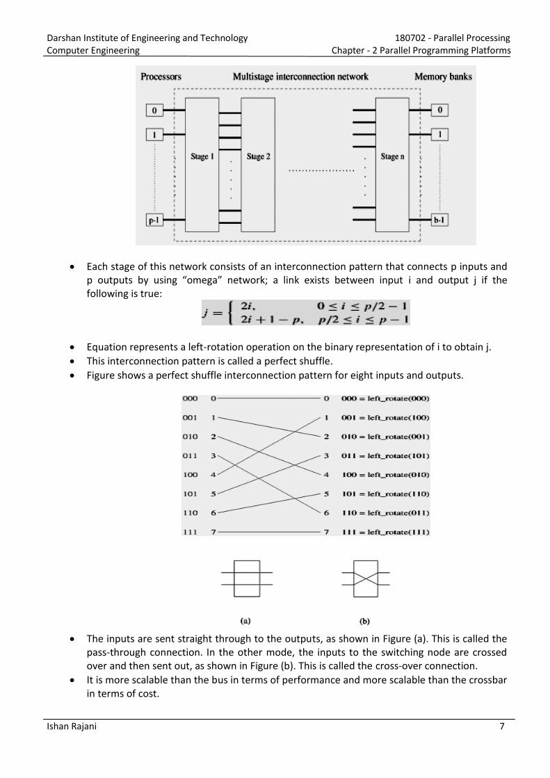
Figure, shows data routing over an omega network from processor two (010) to memory
bank seven (111) and from processor six (110) to memory bank four (100).
Communication link AB is used by both communication paths. Thus, in an omega network,
access to a memory bank by a processor may disallow access to another memory bank by
another processor. Networks with this property are referred to as blocking networks.
8) Explain invalidate protocol used for cache coherence in multiprocessor system. OR
Explain cache coherence mechanism in multiprocessor system. [Oct. 13(7 marks)]
In case of shared-address-space computer additional hardware is required to keep multiple
copies of data consistent with each other.
For example, two processors P0 and P1 are connected over a shared bus to globally
accessible memory and both processors load the same variable.
There are now 3 copies of the variable.
Coherence mechanism must ensure that all operations performed on these copies are
serializable.
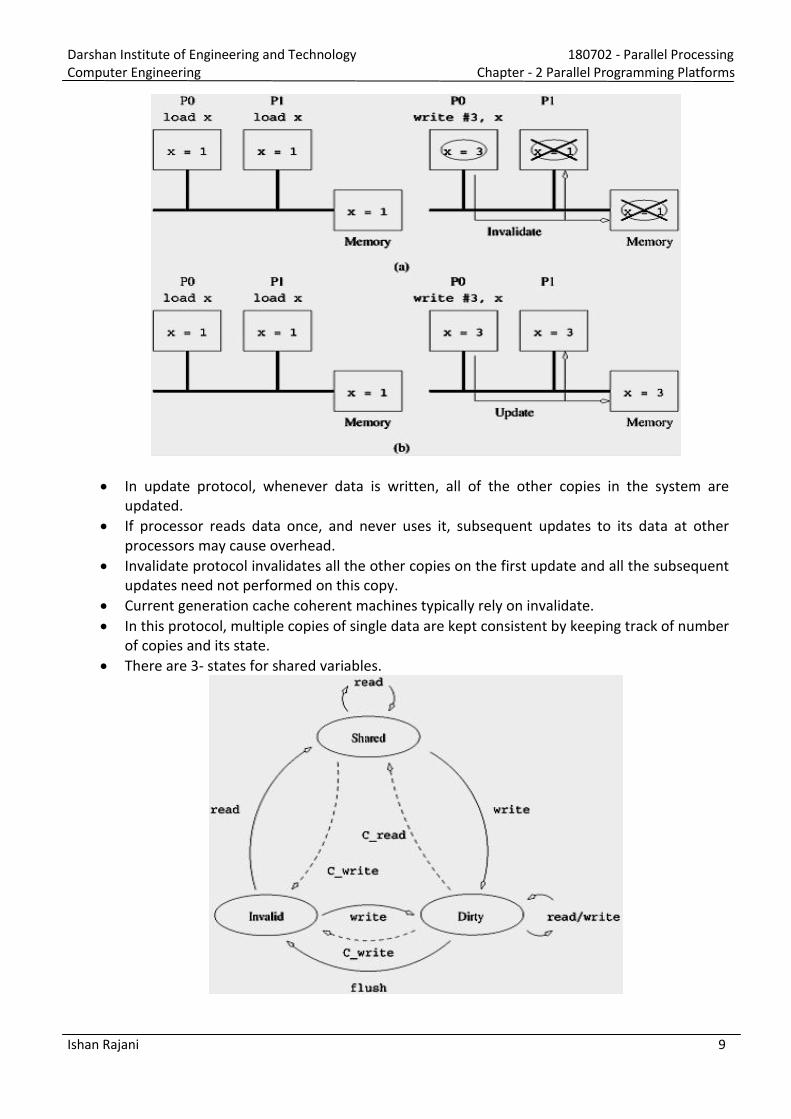
When processor changes the value of its copy, one of two things must happen: 1. other
copies must be invalidated, or 2. other copies must be updated.
Failing this, other processors may work with incorrect value of variable.
This process is shown in the following figure.
There are two protocols referred to as :
o Invalidate
o Update
Darshan Institute of Engineering and Technology 180702 - Parallel Processing
Computer Engineering Chapter - 2 Parallel Programming Platforms
Ishan Rajani 9
In update protocol, whenever data is written, all of the other copies in the system are
updated.
If processor reads data once, and never uses it, subsequent updates to its data at other
processors may cause overhead.
Invalidate protocol invalidates all the other copies on the first update and all the subsequent
updates need not performed on this copy.
Current generation cache coherent machines typically rely on invalidate.
In this protocol, multiple copies of single data are kept consistent by keeping track of number
of copies and its state.
There are 3- states for shared variables.

Darshan Institute of Engineering and Technology 180702 - Parallel Processing
Computer Engineering Chapter - 2 Parallel Programming Platforms
Ishan Rajani 10
Initially variable resides in global memory. When load operation by both processors is
e e uted, the state of aria le is said to e shared . Whe P0 e e utes store o this aria le, it arks all other opies as I alid’ a d its o
op as Dirt . It means all subsequent accesses to this variable will be serviced by P0.
At this point, if P1 attempts to fetch this variable, which was marked dirty by P0, then P0
services the request.
Now, variable at P1 and global memory are updated, and it re-e ters i to “hared state.
Darshan Institute of Engineering and Technology 180702 - Parallel Processing
Computer Engineering Chapter - 3 Principles of Parallel Algorithm Designs
Ishan Rajani 11
1) Enlist various decomposition techniques. Explain data decomposition with suitable example. OR
Explain recursive decomposition technique in detail and draw task dependency graph for the following
se ue ce usi g uick so t ith ecu si e deco positio a d choose 5 as pi ot ele e t i itially. 5, 12, 11, 1, 10, 6, 8, 3, 7, 4, 9, 2 [(Oct. 13, Oct. 12, June 13, June 12) – 7 marks ]
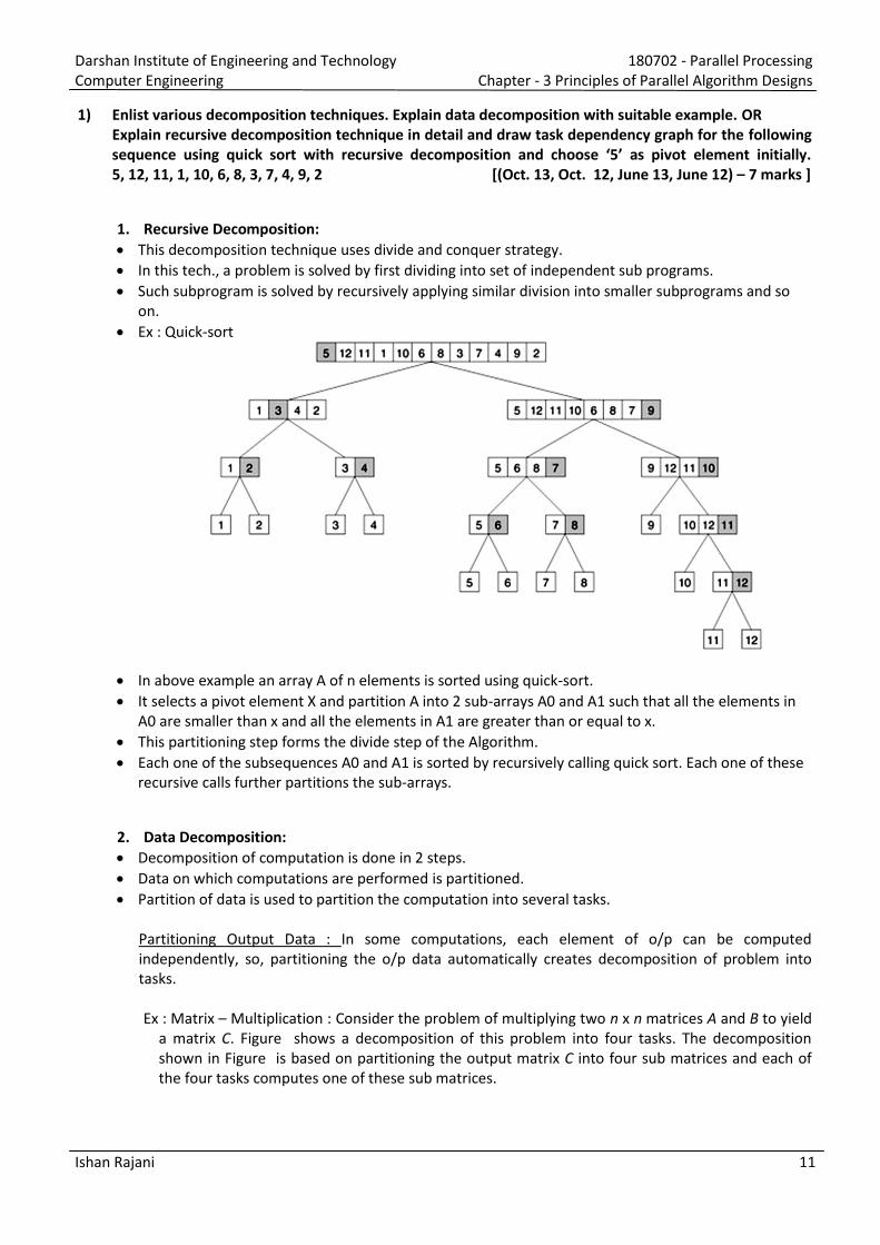
1. Recursive Decomposition:
This decomposition technique uses divide and conquer strategy.
In this tech., a problem is solved by first dividing into set of independent sub programs.
Such subprogram is solved by recursively applying similar division into smaller subprograms and so
on.
Ex : Quick-sort
In above example an array A of n elements is sorted using quick-sort.
It selects a pivot element X and partition A into 2 sub-arrays A0 and A1 such that all the elements in
A0 are smaller than x and all the elements in A1 are greater than or equal to x.
This partitioning step forms the divide step of the Algorithm.
Each one of the subsequences A0 and A1 is sorted by recursively calling quick sort. Each one of these
recursive calls further partitions the sub-arrays.
2. Data Decomposition:
Decomposition of computation is done in 2 steps.
Data on which computations are performed is partitioned.
Partition of data is used to partition the computation into several tasks.
Partitioning Output Data : In some computations, each element of o/p can be computed
independently, so, partitioning the o/p data automatically creates decomposition of problem into
tasks.
Ex : Matrix – Multiplication : Consider the problem of multiplying two n x n matrices A and B to yield
a matrix C. Figure shows a decomposition of this problem into four tasks. The decomposition
shown in Figure is based on partitioning the output matrix C into four sub matrices and each of
the four tasks computes one of these sub matrices.
Darshan Institute of Engineering and Technology 180702 - Parallel Processing
Computer Engineering Chapter - 3 Principles of Parallel Algorithm Designs
Ishan Rajani 12
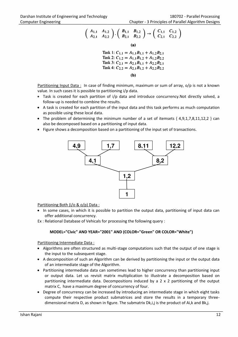
Partitioning Input Data : In case of finding minimum, maximum or sum of array, o/p is not a known
value. In such cases it is possible to partitioning i/p data.
Task is created for each partition of i/p data and introduce concurrency.Not directly solved, a
follow-up is needed to combine the results.
A task is created for each partition of the input data and this task performs as much computation
as possible using these local data.
The problem of determining the minimum number of a set of itemsets { 4,9,1,7,8,11,12,2 } can
also be decomposed based on a partitioning of input data.
Figure shows a decomposition based on a partitioning of the input set of transactions.
Partitioning Both (i/o & o/p) Data :
In some cases, in which it is possible to partition the output data, partitioning of input data can
offer additional concurrency.
Ex : Relational Database of Vehicals for processing the following query :
MODEL="Civic" AND YEAR="2001" AND (COLOR="Green" OR COLOR="White")
Partitioning Intermediate Data :
Algorithms are often structured as multi-stage computations such that the output of one stage is
the input to the subsequent stage.
A decomposition of such an Algorithm can be derived by partitioning the input or the output data
of an intermediate stage of the Algorithm.
Partitioning intermediate data can sometimes lead to higher concurrency than partitioning input
or output data. Let us revisit matrix multiplication to illustrate a decomposition based on
partitioning intermediate data. Decompositions induced by a 2 x 2 partitioning of the output
matrix C, have a maximum degree of concurrency of four.
Degree of concurrency can be increased by introducing an intermediate stage in which eight tasks
compute their respective product submatrices and store the results in a temporary three-
dimensional matrix D, as shown in figure. The submatrix Dk,i,j is the product of Ai,k and Bk,j.
4,9 1,7 12,2 8,11
8,2 4,1
1,2
1
Darshan Institute of Engineering and Technology 180702 - Parallel Processing
Computer Engineering Chapter - 3 Principles of Parallel Algorithm Designs
Ishan Rajani 13
A partitioning of the intermediate matrix D induces a decomposition into eight tasks.After the
multiplication phase, a relatively inexpensive matrix addition step can compute the result matrix C.
3. Exploratory Decomposition:
Exploratory decomposition is used to decompose problems whose underlying computations
correspond to a search of a space for solutions.
In exploratory decomposition, we partition the search space into smaller parts, and search each one
of these parts concurrently, until the desired solutions are found.
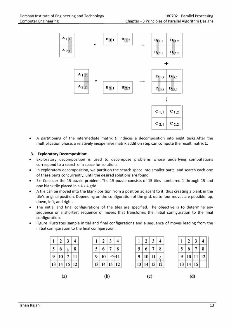
Ex: Consider the 15-puzzle problem. The 15-puzzle consists of 15 tiles numbered 1 through 15 and
one blank tile placed in a 4 x 4 grid.
A tile can be moved into the blank position from a position adjacent to it, thus creating a blank in the
tile's original position. Depending on the configuration of the grid, up to four moves are possible: up,
down, left, and right.
The initial and final configurations of the tiles are specified. The objective is to determine any
sequence or a shortest sequence of moves that transforms the initial configuration to the final
configuration.
Figure illustrates sample initial and final configurations and a sequence of moves leading from the
initial configuration to the final configuration.
Darshan Institute of Engineering and Technology 180702 - Parallel Processing
Computer Engineering Chapter - 3 Principles of Parallel Algorithm Designs
Ishan Rajani 14
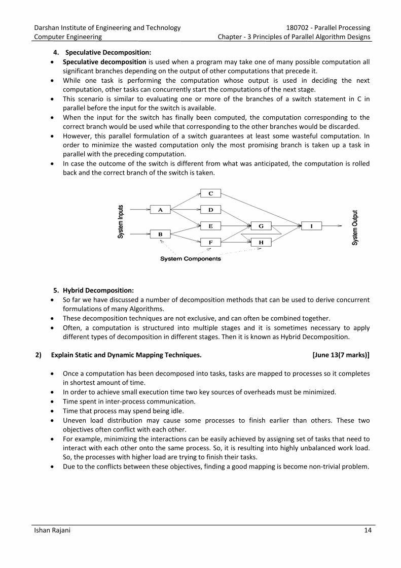
4. Speculative Decomposition:
Speculative decomposition is used when a program may take one of many possible computation all
significant branches depending on the output of other computations that precede it.
While one task is performing the computation whose output is used in deciding the next
computation, other tasks can concurrently start the computations of the next stage.
This scenario is similar to evaluating one or more of the branches of a switch statement in C in
parallel before the input for the switch is available.
When the input for the switch has finally been computed, the computation corresponding to the
correct branch would be used while that corresponding to the other branches would be discarded.
However, this parallel formulation of a switch guarantees at least some wasteful computation. In
order to minimize the wasted computation only the most promising branch is taken up a task in
parallel with the preceding computation.
In case the outcome of the switch is different from what was anticipated, the computation is rolled
back and the correct branch of the switch is taken.
5. Hybrid Decomposition:
So far we have discussed a number of decomposition methods that can be used to derive concurrent
formulations of many Algorithms.
These decomposition techniques are not exclusive, and can often be combined together.
Often, a computation is structured into multiple stages and it is sometimes necessary to apply
different types of decomposition in different stages. Then it is known as Hybrid Decomposition.
2) Explain Static and Dynamic Mapping Techniques. [June 13(7 marks)]
Once a computation has been decomposed into tasks, tasks are mapped to processes so it completes
in shortest amount of time.
In order to achieve small execution time two key sources of overheads must be minimized.
Time spent in inter-process communication.
Time that process may spend being idle.
Uneven load distribution may cause some processes to finish earlier than others. These two
objectives often conflict with each other.
For example, minimizing the interactions can be easily achieved by assigning set of tasks that need to
interact with each other onto the same process. So, it is resulting into highly unbalanced work load.
So, the processes with higher load are trying to finish their tasks.
Due to the conflicts between these objectives, finding a good mapping is become non-trivial problem.
Darshan Institute of Engineering and Technology 180702 - Parallel Processing
Computer Engineering Chapter - 3 Principles of Parallel Algorithm Designs
Ishan Rajani 15
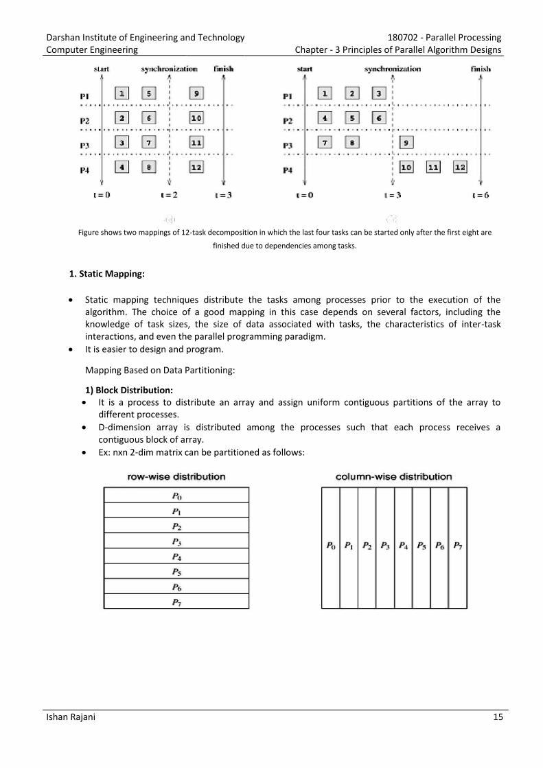
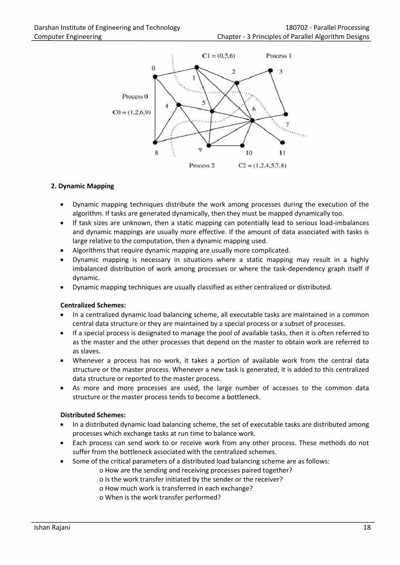
Figure shows two mappings of 12-task decomposition in which the last four tasks can be started only after the first eight are
finished due to dependencies among tasks.
1. Static Mapping:
Static mapping techniques distribute the tasks among processes prior to the execution of the
algorithm. The choice of a good mapping in this case depends on several factors, including the
knowledge of task sizes, the size of data associated with tasks, the characteristics of inter-task
interactions, and even the parallel programming paradigm.
It is easier to design and program. Mapping Based on Data Partitioning: 1) Block Distribution:
It is a process to distribute an array and assign uniform contiguous partitions of the array to
different processes.
D-dimension array is distributed among the processes such that each process receives a
contiguous block of array.
Ex: nxn 2-dim matrix can be partitioned as follows:
Darshan Institute of Engineering and Technology 180702 - Parallel Processing
Computer Engineering Chapter - 3 Principles of Parallel Algorithm Designs
Ishan Rajani 16
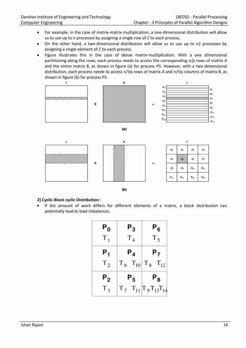
For example, in the case of matrix-matrix multiplication, a one-dimensional distribution will allow
us to use up to n processes by assigning a single row of C to each process.
On the other hand, a two-dimensional distribution will allow us to use up to n2 processes by
assigning a single element of C to each process.
Figure illustrates this in the case of dense matrix-multiplication. With a one dimensional
partitioning along the rows, each process needs to access the corresponding n/p rows of matrix A
and the entire matrix B, as shown in figure (a) for process P5. However, with a two-dimensional
distribution, each process needs to access n/Vp rows of matrix A and n/Vp columns of matrix B, as
shown in figure (b) for process P5.
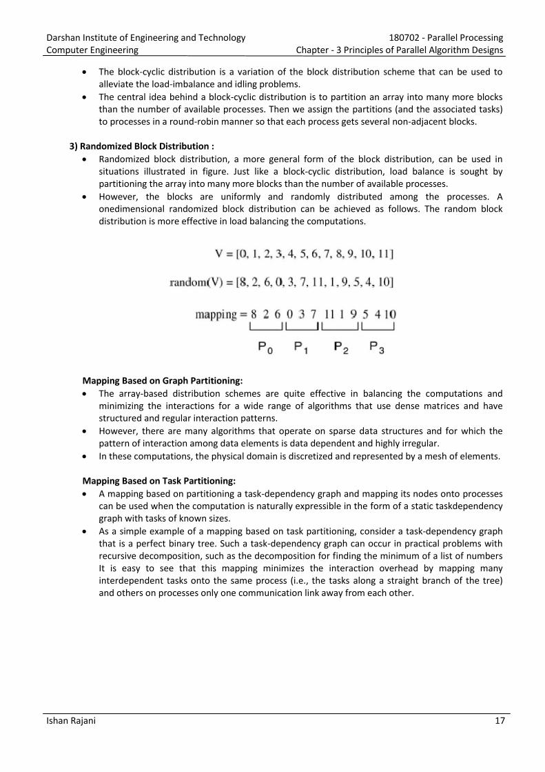
2) Cyclic-Block cyclic Distribution :
If the amount of work differs for different elements of a matrix, a block distribution can
potentially lead to load imbalances.
Darshan Institute of Engineering and Technology 180702 - Parallel Processing
Computer Engineering Chapter - 3 Principles of Parallel Algorithm Designs
Ishan Rajani 17
The block-cyclic distribution is a variation of the block distribution scheme that can be used to
alleviate the load-imbalance and idling problems.
The central idea behind a block-cyclic distribution is to partition an array into many more blocks
than the number of available processes. Then we assign the partitions (and the associated tasks)
to processes in a round-robin manner so that each process gets several non-adjacent blocks.
3) Randomized Block Distribution :
Randomized block distribution, a more general form of the block distribution, can be used in
situations illustrated in figure. Just like a block-cyclic distribution, load balance is sought by
partitioning the array into many more blocks than the number of available processes.
However, the blocks are uniformly and randomly distributed among the processes. A
onedimensional randomized block distribution can be achieved as follows. The random block
distribution is more effective in load balancing the computations.
Mapping Based on Graph Partitioning:
The array-based distribution schemes are quite effective in balancing the computations and
minimizing the interactions for a wide range of algorithms that use dense matrices and have
structured and regular interaction patterns.
However, there are many algorithms that operate on sparse data structures and for which the
pattern of interaction among data elements is data dependent and highly irregular.
In these computations, the physical domain is discretized and represented by a mesh of elements.
Mapping Based on Task Partitioning:
A mapping based on partitioning a task-dependency graph and mapping its nodes onto processes
can be used when the computation is naturally expressible in the form of a static taskdependency
graph with tasks of known sizes.
As a simple example of a mapping based on task partitioning, consider a task-dependency graph
that is a perfect binary tree. Such a task-dependency graph can occur in practical problems with
recursive decomposition, such as the decomposition for finding the minimum of a list of numbers
It is easy to see that this mapping minimizes the interaction overhead by mapping many
interdependent tasks onto the same process (i.e., the tasks along a straight branch of the tree)
and others on processes only one communication link away from each other.
Darshan Institute of Engineering and Technology 180702 - Parallel Processing
Computer Engineering Chapter - 3 Principles of Parallel Algorithm Designs
Ishan Rajani 18
2. Dynamic Mapping
Dynamic mapping techniques distribute the work among processes during the execution of the
algorithm. If tasks are generated dynamically, then they must be mapped dynamically too.
If task sizes are unknown, then a static mapping can potentially lead to serious load-imbalances
and dynamic mappings are usually more effective. If the amount of data associated with tasks is
large relative to the computation, then a dynamic mapping used.
Algorithms that require dynamic mapping are usually more complicated.
Dynamic mapping is necessary in situations where a static mapping may result in a highly
imbalanced distribution of work among processes or where the task-dependency graph itself if
dynamic.
Dynamic mapping techniques are usually classified as either centralized or distributed.
Centralized Schemes:
In a centralized dynamic load balancing scheme, all executable tasks are maintained in a common
central data structure or they are maintained by a special process or a subset of processes.
If a special process is designated to manage the pool of available tasks, then it is often referred to
as the master and the other processes that depend on the master to obtain work are referred to
as slaves.
Whenever a process has no work, it takes a portion of available work from the central data
structure or the master process. Whenever a new task is generated, it is added to this centralized
data structure or reported to the master process.
As more and more processes are used, the large number of accesses to the common data
structure or the master process tends to become a bottleneck.
Distributed Schemes:
In a distributed dynamic load balancing scheme, the set of executable tasks are distributed among
processes which exchange tasks at run time to balance work.
Each process can send work to or receive work from any other process. These methods do not
suffer from the bottleneck associated with the centralized schemes.
Some of the critical parameters of a distributed load balancing scheme are as follows:
o How are the sending and receiving processes paired together?
o Is the work transfer initiated by the sender or the receiver?
o How much work is transferred in each exchange?
o When is the work transfer performed?
Darshan Institute of Engineering and Technology 180702 - Parallel Processing
Computer Engineering Chapter - 3 Principles of Parallel Algorithm Designs
Ishan Rajani 19
3) Explain various parallel algorithm models. [Oct. 12(7 marks)]
An algorithm model is typically a way of structuring a parallel algorithm by selecting decomposition
and mapping technique and applying the appropriate strategy to minimize interactions.
1) Data Parallel Model:
The data-parallel model is one of the simplest algorithm models. In this model, the tasks are statically
or semi-statically mapped onto processes and each task performs similar operations on different
data.
This type of parallelism that is a result of identical operations being applied concurrently on different
data items is called data parallelism.
Data-parallel algorithms can be implemented in both shared-address-space and message passing
paradigms.
However, the partitioned address-space in a message-passing paradigm may allow better control of
placement, and thus may offer a better handle on locality.
Interaction overheads in the data-parallel model can be minimized by choosing a locality preserving
decomposition and, if applicable, by overlapping computation and interaction and by using optimized
collective interaction routines.
A key characteristic of data-parallel problems is that for most problems, the degree of data
parallelism increases with the size of the problem, making it possible to use more processes to
effectively solve larger problems.
2) Task Graph Model:
As the computations in any parallel algorithm can be viewed as a task- dependency graph. However,
in certain parallel algorithms, the task-dependency graph is explicitly used in mapping.
In the task graph model, the interrelationships among the tasks are utilized to promote locality or to
reduce interaction costs.
This model is typically employed to solve problems in which the amount of data associated with the
tasks is large relative to the amount of computation associated with them.
Typical interaction-reducing techniques applicable to this model include reducing the volume and
frequency of interaction by promoting locality while mapping the tasks based on the interaction
pattern of tasks, and using asynchronous interaction methods to overlap the interaction with
computation.
Examples of algorithms based on the task graph model include parallel quicksort, sparse matrix
factorization, and many parallel algorithms derived via divide-and-conquer decomposition.
This type of parallelism that is naturally expressed by independent tasks in a task-dependency graph
is called task parallelism.
3) Work Pool Model:
The work pool or the task pool model is characterized by a dynamic mapping of tasks onto processes
for load balancing in which any task may potentially be performed by any process.
There is no desired pre-mapping of tasks onto processes. The mapping may be centralized or
decentralized.
The work may be statically available in the beginning, or could be dynamically generated; i.e., the
processes may generate work and add it to the global (possibly distributed) work pool.
If the work is generated dynamically and a decentralized mapping is used, then a termination
detection algorithm would be required so that all processes can actually detect the completion of the
entire program and stop looking for more work.
In the message-passing paradigm, the work pool model is typically used when the amount of data
associated with tasks is relatively small compared to the computation associated with the tasks.
Darshan Institute of Engineering and Technology 180702 - Parallel Processing
Computer Engineering Chapter - 3 Principles of Parallel Algorithm Designs
Ishan Rajani 20
4) Master-Slave Model:
In the master-slave or the manager-worker model, one or more master processes generate work and
allocate it to worker processes. The tasks may be allocated a priori if the manager can estimate the
size of the tasks or if a random mapping can do an adequate job of load balancing.
In another scenario, workers are assigned smaller pieces of work at different times. The latter scheme
is preferred if it is time consuming for the master to generate work and hence it is not desirable to
make all workers wait until the master has generated all work pieces.
The manager-worker model can be generalized to the hierarchical or multi-level managerworker
model in which the top-level manager feeds large chunks of tasks to second-level managers, who
further subdivide the tasks among their own workers and may perform part of the work themselves.
This model is generally equally suitable to shared-address-space or message-passing paradigms.
The manager needs to give out work and workers need to get work from the manager. While using
the master-slave model, care should be taken to ensure that the master does not become a
bottleneck, which may happen if the tasks are too small or the workers are relatively fast.
5) Pipeline Model:
In the pipeline model, a stream of data is passed on through a succession of processes, each of which
performs some task on it.
This simultaneous execution of different programs on a data stream is called stream parallelism.
A new data triggers the execution of a new task by a process in the pipeline. A pipeline is a chain of
producers and consumers. Each process in the pipeline can be viewed as a consumer of a sequence of
data items for the process preceding it in the pipeline and as a producer of data for the process
following it in the pipeline.
The pipeline does not need to be a linear chain; it can be a directed graph. The pipeline model usually
involves a static mapping of tasks onto processes.
The most common interaction reduction technique applicable to this model is overlapping interaction
with computation.
6) Hybrid Model:
In some cases, more than one model may be applicable to the problem at hand, resulting in a hybrid
algorithm model.
A hybrid model may be composed either of multiple models applied hierarchically or multiple models
applied sequentially to different phases of a parallel algorithm.
Darshan Institute of Engineering and Technology 180702 – Parallel Processing
Computer Engineering Chapter - 4 Basic communication operations and algorithms
Ishan Rajani 21
1. Explain One-To-All broadcasting in different structures. [June 12(3.5 marks)]
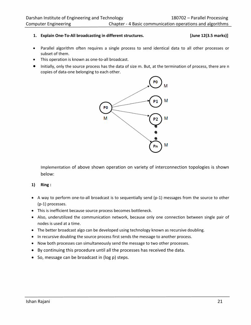
Parallel algorithm often requires a single process to send identical data to all other processes or
subset of them.
This operation is known as one-to-all broadcast.
Initially, only the source process has the data of size m. But, at the termination of process, there are n
copies of data-one belonging to each other.
Implementation of above shown operation on variety of interconnection topologies is shown
below:
1) Ring :
A way to perform one-to-all broadcast is to sequentially send (p-1) messages from the source to other
(p-1) processes.
This is inefficient because source process becomes bottleneck.
Also, underutilized the communication network, because only one connection between single pair of
nodes is used at a time.
The better broadcast algo can be developed using technology known as recursive doubling.
In recursive doubling the source process first sends the message to another process.
Now both processes can simultaneously send the message to two other processes.
By continuing this procedure until all the processes has received the data.
So, message can be broadcast in (log p) steps.
Darshan Institute of Engineering and Technology 180702 – Parallel Processing
Computer Engineering Chapter - 4 Basic communication operations and algorithms
Ishan Rajani 22
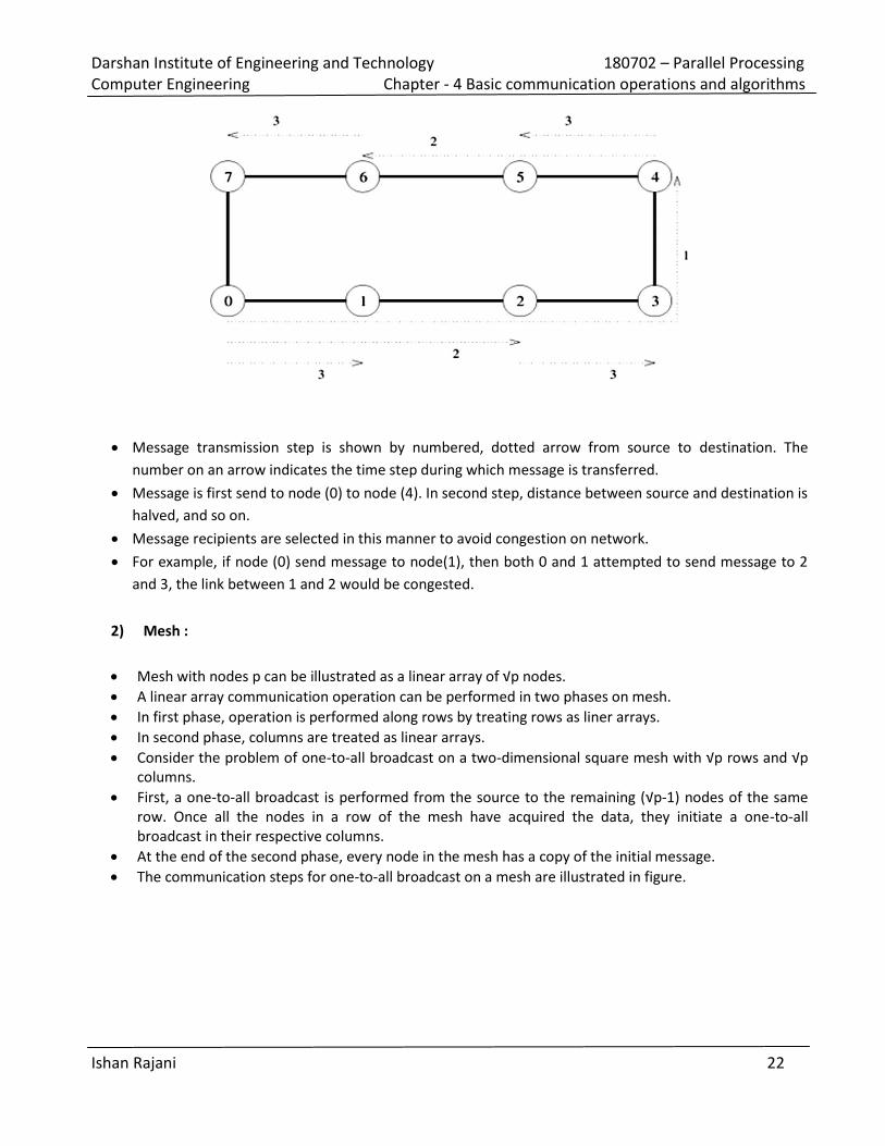
Message transmission step is shown by numbered, dotted arrow from source to destination. The
number on an arrow indicates the time step during which message is transferred.
Message is first send to node (0) to node (4). In second step, distance between source and destination is
halved, and so on.
Message recipients are selected in this manner to avoid congestion on network.
For example, if node (0) send message to node(1), then both 0 and 1 attempted to send message to 2
and 3, the link between 1 and 2 would be congested.
2) Mesh :
Mesh with nodes p can e illustrated as a linear array of √p nodes. A linear array communication operation can be performed in two phases on mesh.
In first phase, operation is performed along rows by treating rows as liner arrays.
In second phase, columns are treated as linear arrays.
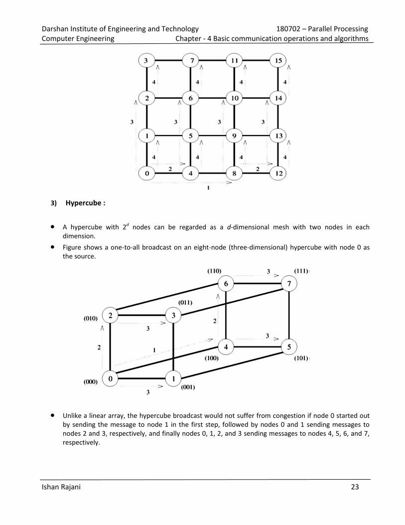
Consider the problem of one-to-all broadcast on a two-dimensional square mesh with √p rows and √p
columns.
First, a one-to-all broadcast is performed from the source to the remaining (√p-1) nodes of the same
row. Once all the nodes in a row of the mesh have acquired the data, they initiate a one-to-all
broadcast in their respective columns.
At the end of the second phase, every node in the mesh has a copy of the initial message.
The communication steps for one-to-all broadcast on a mesh are illustrated in figure.
Darshan Institute of Engineering and Technology 180702 – Parallel Processing
Computer Engineering Chapter - 4 Basic communication operations and algorithms
Ishan Rajani 23
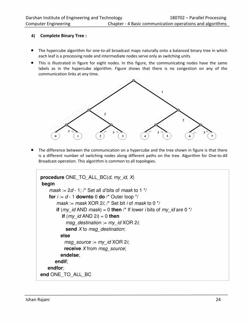
3) Hypercube :
A hypercube with 2d nodes can be regarded as a d-dimensional mesh with two nodes in each
dimension.
Figure shows a one-to-all broadcast on an eight-node (three-dimensional) hypercube with node 0 as
the source.
Unlike a linear array, the hypercube broadcast would not suffer from congestion if node 0 started out
by sending the message to node 1 in the first step, followed by nodes 0 and 1 sending messages to
nodes 2 and 3, respectively, and finally nodes 0, 1, 2, and 3 sending messages to nodes 4, 5, 6, and 7,
respectively.
Darshan Institute of Engineering and Technology 180702 – Parallel Processing
Computer Engineering Chapter - 4 Basic communication operations and algorithms
Ishan Rajani 24
4) Complete Binary Tree :
The hypercube algorithm for one-to-all broadcast maps naturally onto a balanced binary tree in which
each leaf is a processing node and intermediate nodes serve only as switching units.
This is illustrated in figure for eight nodes. In this figure, the communicating nodes have the same
labels as in the hypercube algorithm. Figure shows that there is no congestion on any of the
communication links at any time.
The difference between the communication on a hypercube and the tree shown in figure is that there
is a different number of switching nodes along different paths on the tree. Algorithm for One-to-All
Broadcast operation. This algorithm is common to all topologies.
procedure ONE_TO_ALL_BC(d, my_id, X)
begin
mask := 2d - 1; /* Set all d bits of mask to 1 */
for i := d - 1 downto 0 do /* Outer loop */
mask := mask XOR 2i; /* Set bit i of mask to 0 */
if (my_id AND mask) = 0 then /* If lower i bits of my_id are 0 */
if (my_id AND 2i) = 0 then
msg_destination := my_id XOR 2i;
send X to msg_destination;
else
msg_source := my_id XOR 2i;
receive X from msg_source;
endelse;
endif;
endfor;
end ONE_TO_ALL_BC
Darshan Institute of Engineering and Technology 180702 – Parallel Processing
Computer Engineering Chapter - 4 Basic communication operations and algorithms
Ishan Rajani 25
2. What is dual operation? Explain dual operation of one-to-all broadcast in different structures.
[June 12(3.5 marks)]
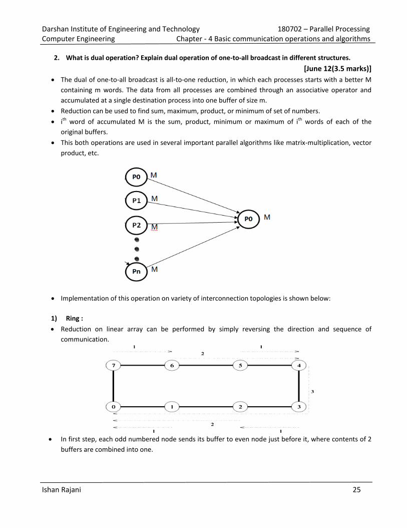
The dual of one-to-all broadcast is all-to-one reduction, in which each processes starts with a better M
containing m words. The data from all processes are combined through an associative operator and
accumulated at a single destination process into one buffer of size m.
Reduction can be used to find sum, maximum, product, or minimum of set of numbers.
ith
word of accumulated M is the sum, product, minimum or maximum of ith
words of each of the
original buffers.
This both operations are used in several important parallel algorithms like matrix-multiplication, vector
product, etc.
Implementation of this operation on variety of interconnection topologies is shown below:
1) Ring :
Reduction on linear array can be performed by simply reversing the direction and sequence of
communication.
In first step, each odd numbered node sends its buffer to even node just before it, where contents of 2
buffers are combined into one.
Darshan Institute of Engineering and Technology 180702 – Parallel Processing
Computer Engineering Chapter - 4 Basic communication operations and algorithms
Ishan Rajani 26
In second step, there are now 4 buffers left to reduce on nodes 0, 2, 4, & 6. Content of buffer 0 and 2
are combined on 0 and nodes 6 and 4 are combined on 4.
Finally, 4 send its buffer to 0 which computes the final result of reduction.
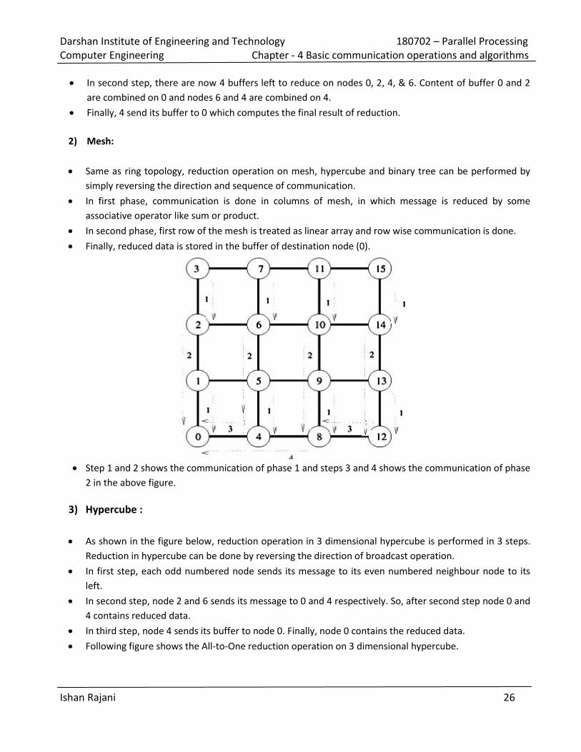
2) Mesh:
Same as ring topology, reduction operation on mesh, hypercube and binary tree can be performed by
simply reversing the direction and sequence of communication.
In first phase, communication is done in columns of mesh, in which message is reduced by some
associative operator like sum or product.
In second phase, first row of the mesh is treated as linear array and row wise communication is done.
Finally, reduced data is stored in the buffer of destination node (0).
Step 1 and 2 shows the communication of phase 1 and steps 3 and 4 shows the communication of phase
2 in the above figure.
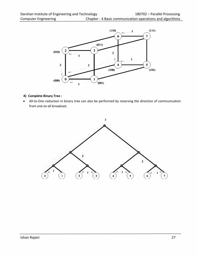
3) Hypercube :
As shown in the figure below, reduction operation in 3 dimensional hypercube is performed in 3 steps.
Reduction in hypercube can be done by reversing the direction of broadcast operation.
In first step, each odd numbered node sends its message to its even numbered neighbour node to its
left.
In second step, node 2 and 6 sends its message to 0 and 4 respectively. So, after second step node 0 and
4 contains reduced data.
In third step, node 4 sends its buffer to node 0. Finally, node 0 contains the reduced data.
Following figure shows the All-to-One reduction operation on 3 dimensional hypercube.
Darshan Institute of Engineering and Technology 180702 – Parallel Processing
Computer Engineering Chapter - 4 Basic communication operations and algorithms
Ishan Rajani 27
4) Complete Binary Tree :
All-to-One reduction in binary tree can also be performed by reversing the direction of communication
from one-to-all broadcast.
Darshan Institute of Engineering and Technology 180702 – Parallel Processing
Computer Engineering Chapter - 4 Basic communication operations and algorithms
Ishan Rajani 28
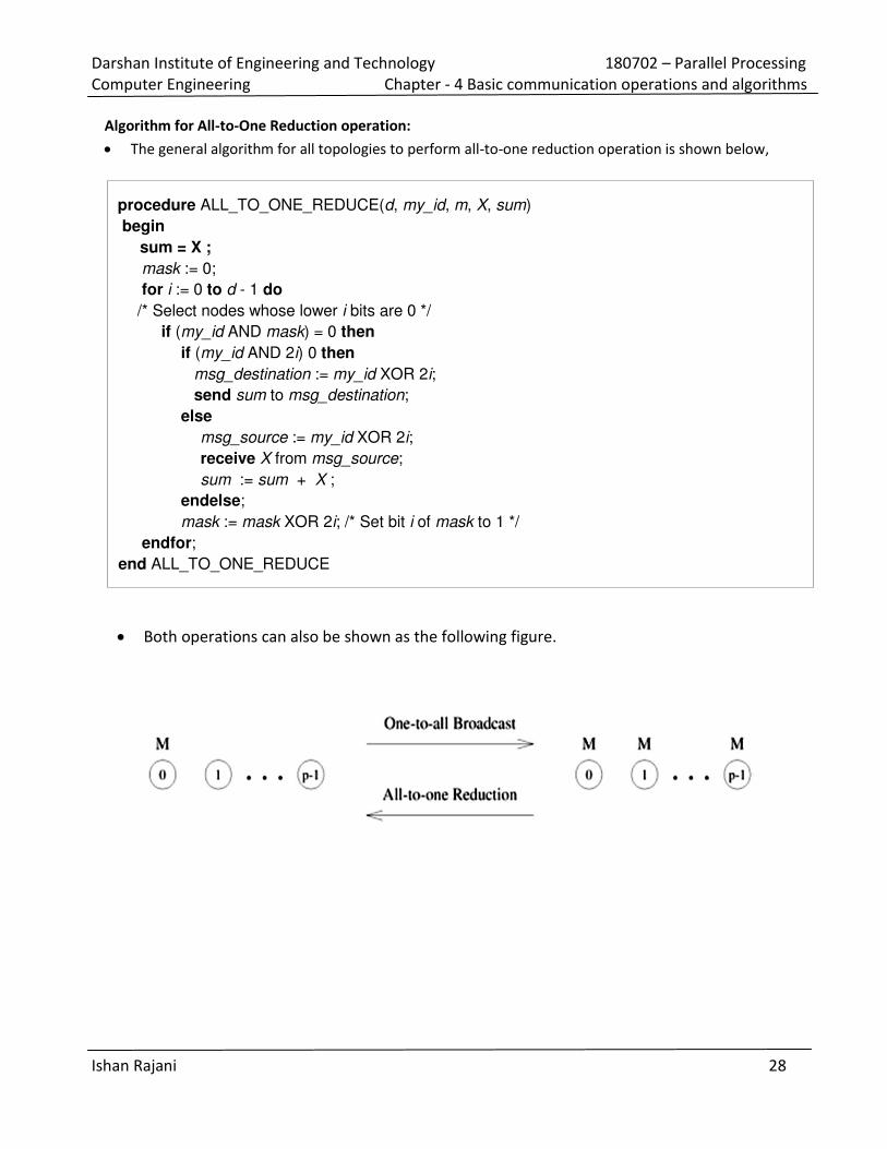
Algorithm for All-to-One Reduction operation:
The general algorithm for all topologies to perform all-to-one reduction operation is shown below,
procedure ALL_TO_ONE_REDUCE(d, my_id, m, X, sum)
begin
sum = X ;
mask := 0;
for i := 0 to d - 1 do
/* Select nodes whose lower i bits are 0 */
if (my_id AND mask) = 0 then
if (my_id AND 2i) 0 then
msg_destination := my_id XOR 2i;
send sum to msg_destination;
else
msg_source := my_id XOR 2i;
receive X from msg_source;
sum := sum + X ;
endelse;
mask := mask XOR 2i; /* Set bit i of mask to 1 */
endfor;
end ALL_TO_ONE_REDUCE
Both operations can also be shown as the following figure.
Darshan Institute of Engineering and Technology 180702 – Parallel Processing
Computer Engineering Chapter - 4 Basic communication operations and algorithms
Ishan Rajani 29
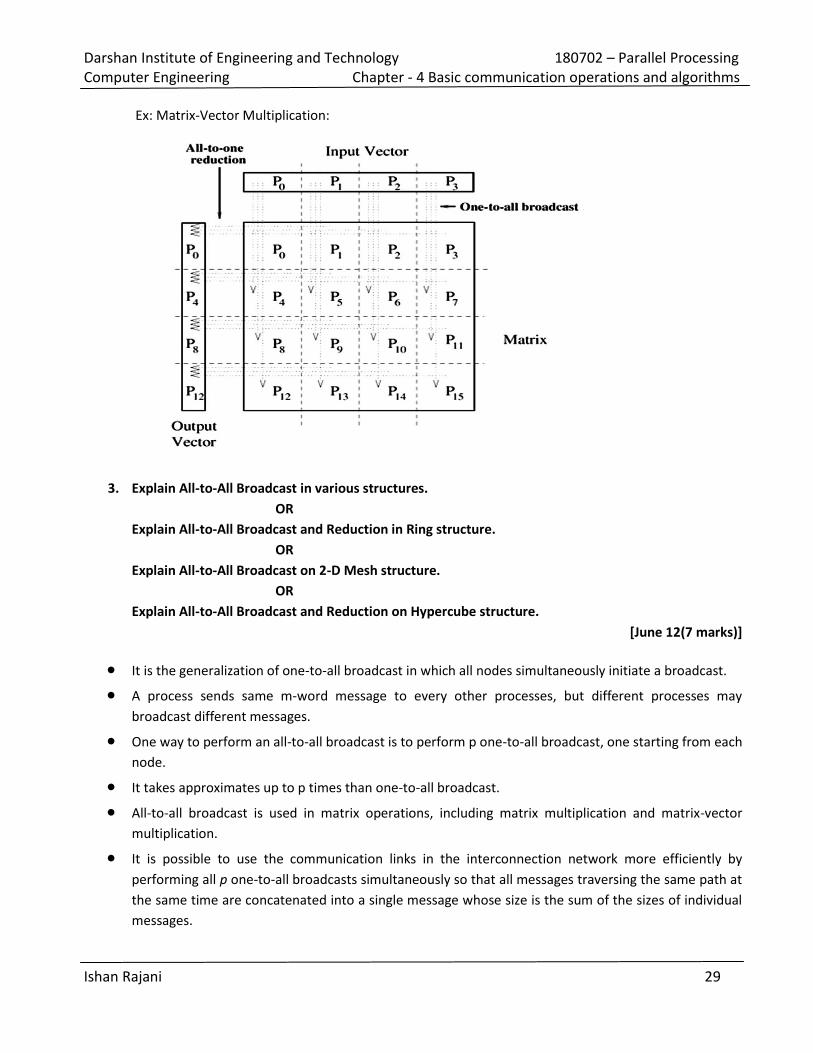
Ex: Matrix-Vector Multiplication:
3. Explain All-to-All Broadcast in various structures.
OR
Explain All-to-All Broadcast and Reduction in Ring structure.
OR
Explain All-to-All Broadcast on 2-D Mesh structure.
OR
Explain All-to-All Broadcast and Reduction on Hypercube structure.
[June 12(7 marks)]
It is the generalization of one-to-all broadcast in which all nodes simultaneously initiate a broadcast.
A process sends same m-word message to every other processes, but different processes may
broadcast different messages.
One way to perform an all-to-all broadcast is to perform p one-to-all broadcast, one starting from each
node.
It takes approximates up to p times than one-to-all broadcast.
All-to-all broadcast is used in matrix operations, including matrix multiplication and matrix-vector
multiplication.
It is possible to use the communication links in the interconnection network more efficiently by
performing all p one-to-all broadcasts simultaneously so that all messages traversing the same path at
the same time are concatenated into a single message whose size is the sum of the sizes of individual
messages.
Darshan Institute of Engineering and Technology 180702 – Parallel Processing
Computer Engineering Chapter - 4 Basic communication operations and algorithms
Ishan Rajani 30
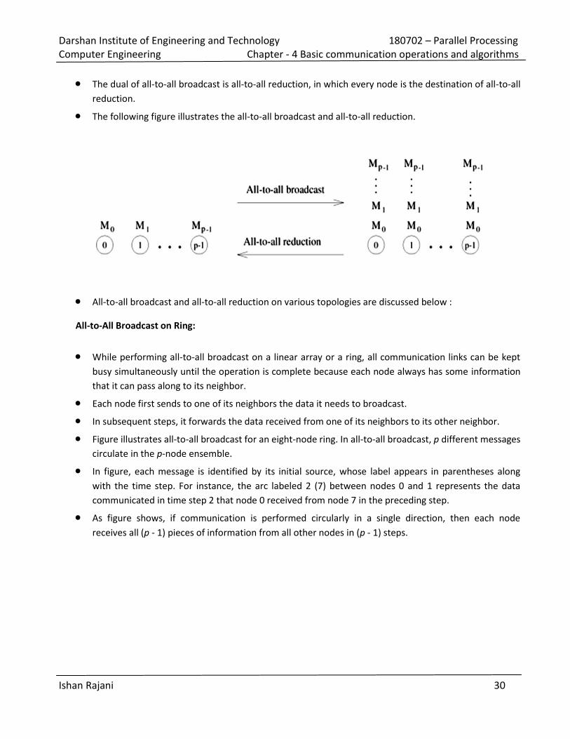
The dual of all-to-all broadcast is all-to-all reduction, in which every node is the destination of all-to-all
reduction.
The following figure illustrates the all-to-all broadcast and all-to-all reduction.
All-to-all broadcast and all-to-all reduction on various topologies are discussed below :
All-to-All Broadcast on Ring:
While performing all-to-all broadcast on a linear array or a ring, all communication links can be kept
busy simultaneously until the operation is complete because each node always has some information
that it can pass along to its neighbor.
Each node first sends to one of its neighbors the data it needs to broadcast.
In subsequent steps, it forwards the data received from one of its neighbors to its other neighbor.
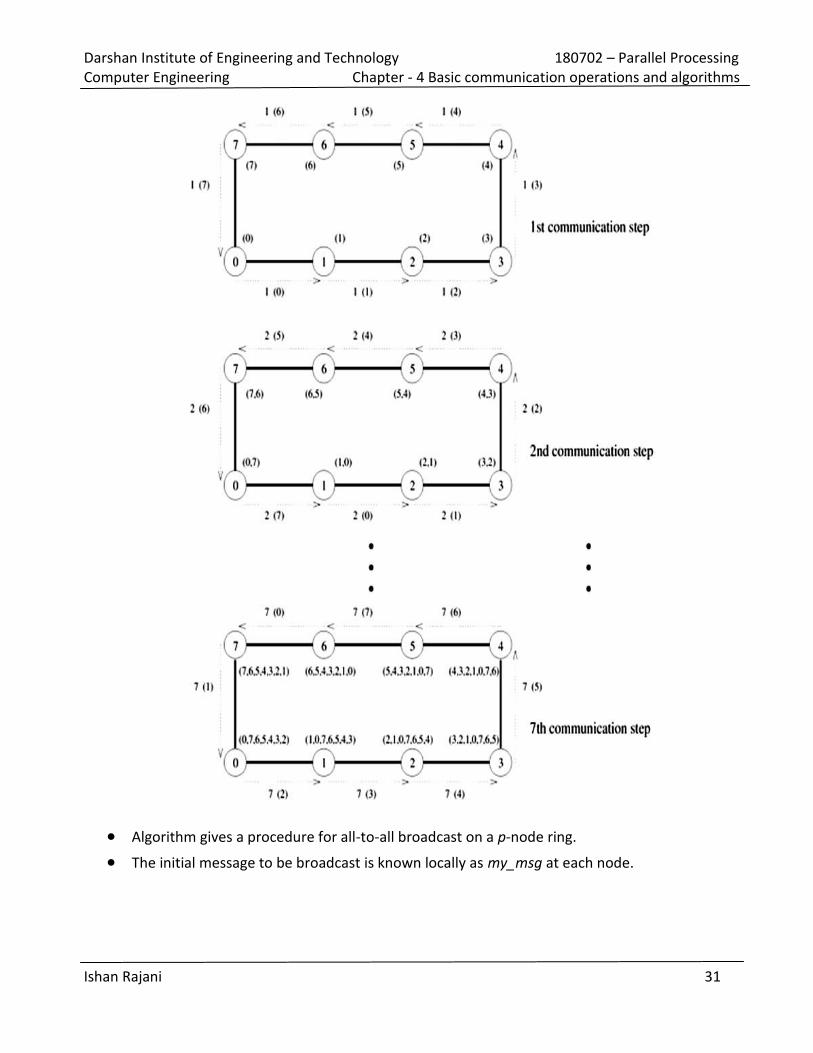
Figure illustrates all-to-all broadcast for an eight-node ring. In all-to-all broadcast, p different messages
circulate in the p-node ensemble.
In figure, each message is identified by its initial source, whose label appears in parentheses along
with the time step. For instance, the arc labeled 2 (7) between nodes 0 and 1 represents the data
communicated in time step 2 that node 0 received from node 7 in the preceding step.
As figure shows, if communication is performed circularly in a single direction, then each node
receives all (p - 1) pieces of information from all other nodes in (p - 1) steps.
Darshan Institute of Engineering and Technology 180702 – Parallel Processing
Computer Engineering Chapter - 4 Basic communication operations and algorithms
Ishan Rajani 31
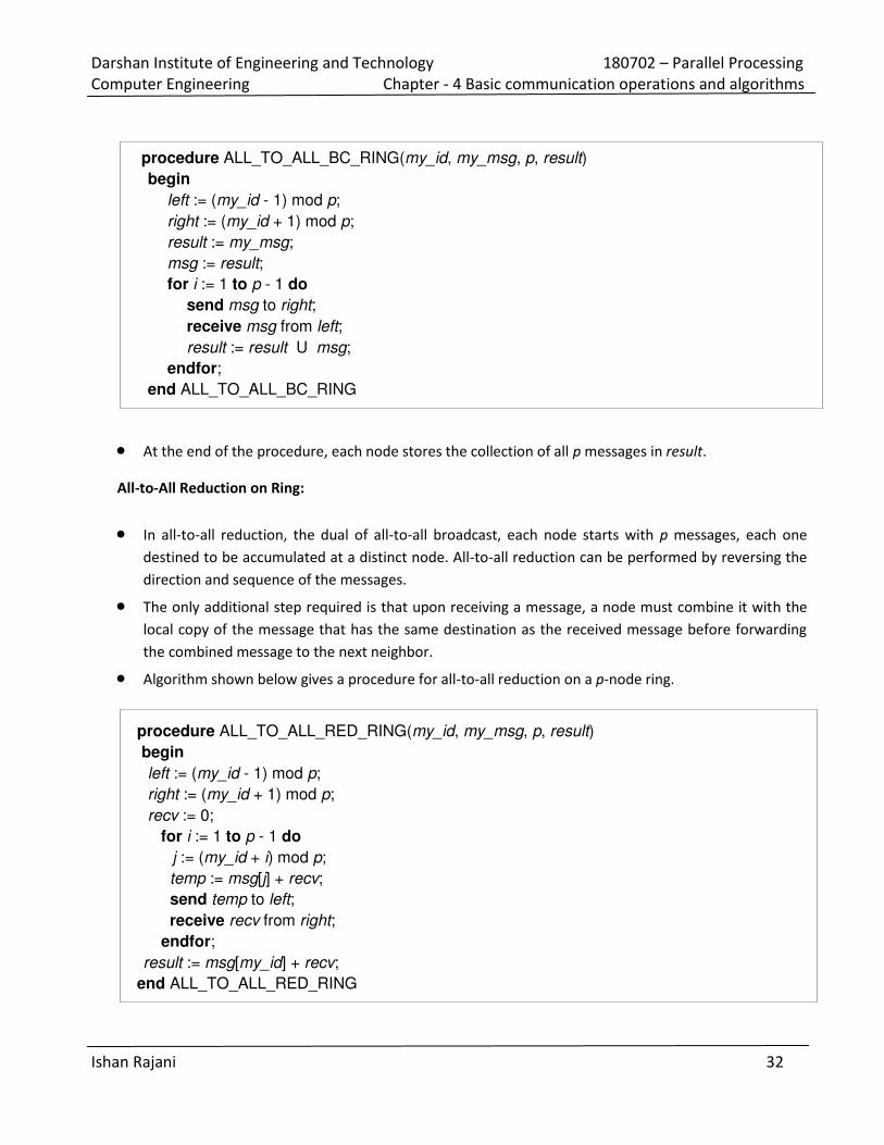
Algorithm gives a procedure for all-to-all broadcast on a p-node ring.
The initial message to be broadcast is known locally as my_msg at each node.
Darshan Institute of Engineering and Technology 180702 – Parallel Processing
Computer Engineering Chapter - 4 Basic communication operations and algorithms
Ishan Rajani 32
procedure ALL_TO_ALL_BC_RING(my_id, my_msg, p, result)
begin
left := (my_id - 1) mod p;
right := (my_id + 1) mod p;
result := my_msg;
msg := result;
for i := 1 to p - 1 do
send msg to right;
receive msg from left;
result := result U msg;
endfor;
end ALL_TO_ALL_BC_RING
At the end of the procedure, each node stores the collection of all p messages in result.
All-to-All Reduction on Ring:
In all-to-all reduction, the dual of all-to-all broadcast, each node starts with p messages, each one
destined to be accumulated at a distinct node. All-to-all reduction can be performed by reversing the
direction and sequence of the messages.
The only additional step required is that upon receiving a message, a node must combine it with the
local copy of the message that has the same destination as the received message before forwarding
the combined message to the next neighbor.
Algorithm shown below gives a procedure for all-to-all reduction on a p-node ring.
procedure ALL_TO_ALL_RED_RING(my_id, my_msg, p, result)
begin
left := (my_id - 1) mod p;
right := (my_id + 1) mod p;
recv := 0;
for i := 1 to p - 1 do
j := (my_id + i) mod p;
temp := msg[j] + recv;
send temp to left;
receive recv from right;
endfor;
result := msg[my_id] + recv;
end ALL_TO_ALL_RED_RING
Darshan Institute of Engineering and Technology 180702 – Parallel Processing
Computer Engineering Chapter - 4 Basic communication operations and algorithms
Ishan Rajani 33
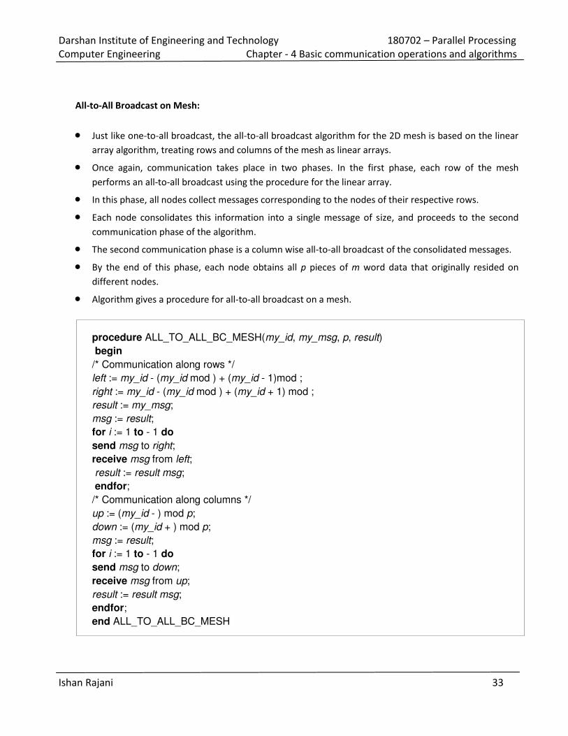
All-to-All Broadcast on Mesh:
Just like one-to-all broadcast, the all-to-all broadcast algorithm for the 2D mesh is based on the linear
array algorithm, treating rows and columns of the mesh as linear arrays.
Once again, communication takes place in two phases. In the first phase, each row of the mesh
performs an all-to-all broadcast using the procedure for the linear array.
In this phase, all nodes collect messages corresponding to the nodes of their respective rows.
Each node consolidates this information into a single message of size, and proceeds to the second
communication phase of the algorithm.
The second communication phase is a column wise all-to-all broadcast of the consolidated messages.
By the end of this phase, each node obtains all p pieces of m word data that originally resided on
different nodes.
Algorithm gives a procedure for all-to-all broadcast on a mesh.
procedure ALL_TO_ALL_BC_MESH(my_id, my_msg, p, result)
begin
/* Communication along rows */
left := my_id - (my_id mod ) + (my_id - 1)mod ;
right := my_id - (my_id mod ) + (my_id + 1) mod ;
result := my_msg;
msg := result;
for i := 1 to - 1 do
send msg to right;
receive msg from left;
result := result msg;
endfor;
/* Communication along columns */
up := (my_id - ) mod p;
down := (my_id + ) mod p;
msg := result;
for i := 1 to - 1 do
send msg to down;
receive msg from up;
result := result msg;
endfor;
end ALL_TO_ALL_BC_MESH
Darshan Institute of Engineering and Technology 180702 – Parallel Processing
Computer Engineering Chapter - 4 Basic communication operations and algorithms
Ishan Rajani 34
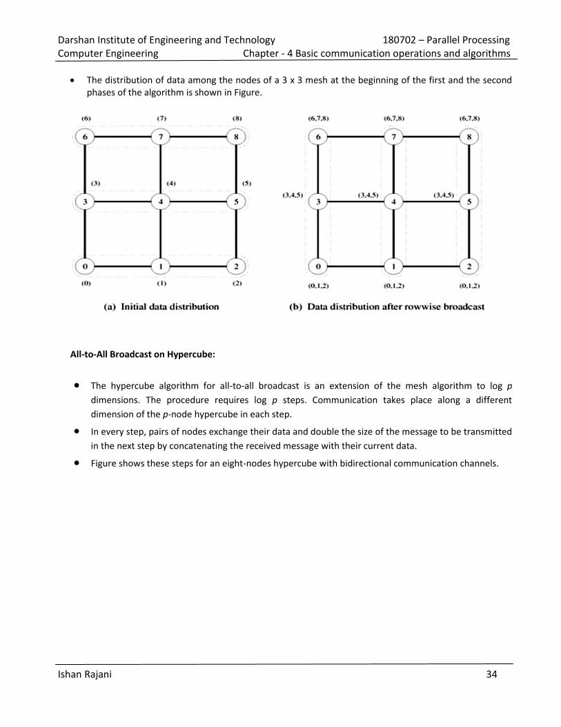
The distribution of data among the nodes of a 3 x 3 mesh at the beginning of the first and the second
phases of the algorithm is shown in Figure.
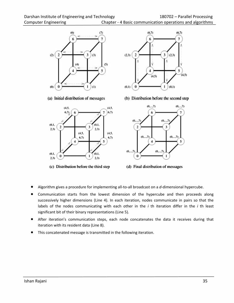
All-to-All Broadcast on Hypercube:
The hypercube algorithm for all-to-all broadcast is an extension of the mesh algorithm to log p
dimensions. The procedure requires log p steps. Communication takes place along a different
dimension of the p-node hypercube in each step.
In every step, pairs of nodes exchange their data and double the size of the message to be transmitted
in the next step by concatenating the received message with their current data.
Figure shows these steps for an eight-nodes hypercube with bidirectional communication channels.
Darshan Institute of Engineering and Technology 180702 – Parallel Processing
Computer Engineering Chapter - 4 Basic communication operations and algorithms
Ishan Rajani 35
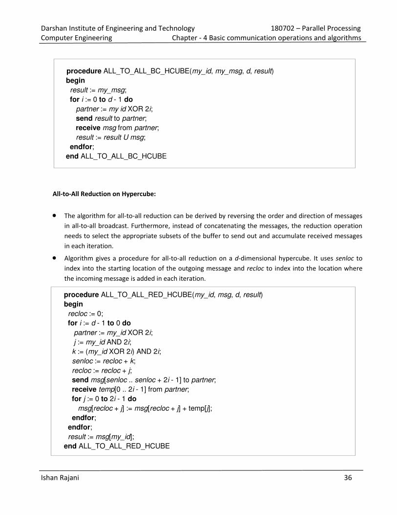
Algorithm gives a procedure for implementing all-to-all broadcast on a d-dimensional hypercube.
Communication starts from the lowest dimension of the hypercube and then proceeds along
successively higher dimensions (Line 4). In each iteration, nodes communicate in pairs so that the
labels of the nodes communicating with each other in the i th iteration differ in the i th least
significant bit of their binary representations (Line 5).
After iteration’s communication steps, each node concatenates the data it receives during that
iteration with its resident data (Line 8).
This concatenated message is transmitted in the following iteration.
Darshan Institute of Engineering and Technology 180702 – Parallel Processing
Computer Engineering Chapter - 4 Basic communication operations and algorithms
Ishan Rajani 36
procedure ALL_TO_ALL_BC_HCUBE(my_id, my_msg, d, result)
begin
result := my_msg;
for i := 0 to d - 1 do
partner := my id XOR 2i;
send result to partner;
receive msg from partner;
result := result U msg;
endfor;
end ALL_TO_ALL_BC_HCUBE
All-to-All Reduction on Hypercube:
The algorithm for all-to-all reduction can be derived by reversing the order and direction of messages
in all-to-all broadcast. Furthermore, instead of concatenating the messages, the reduction operation
needs to select the appropriate subsets of the buffer to send out and accumulate received messages
in each iteration.
Algorithm gives a procedure for all-to-all reduction on a d-dimensional hypercube. It uses senloc to
index into the starting location of the outgoing message and recloc to index into the location where
the incoming message is added in each iteration.
procedure ALL_TO_ALL_RED_HCUBE(my_id, msg, d, result)
begin
recloc := 0;
for i := d - 1 to 0 do
partner := my_id XOR 2i;
j := my_id AND 2i;
k := (my_id XOR 2i) AND 2i;
senloc := recloc + k;
recloc := recloc + j;
send msg[senloc .. senloc + 2i - 1] to partner;
receive temp[0 .. 2i - 1] from partner;
for j := 0 to 2i - 1 do
msg[recloc + j] := msg[recloc + j] + temp[j];
endfor;
endfor;
result := msg[my_id];
end ALL_TO_ALL_RED_HCUBE
Darshan Institute of Engineering and Technology 180702 – Parallel Processing
Computer Engineering Chapter - 4 Basic communication operations and algorithms
Ishan Rajani 37
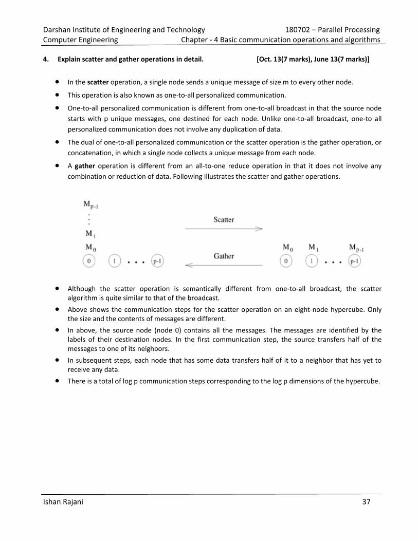
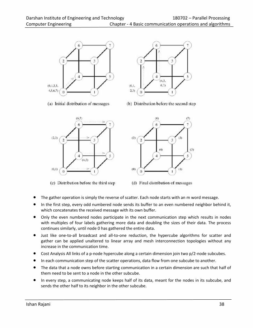
4. Explain scatter and gather operations in detail. [Oct. 13(7 marks), June 13(7 marks)]
In the scatter operation, a single node sends a unique message of size m to every other node.
This operation is also known as one-to-all personalized communication.
One-to-all personalized communication is different from one-to-all broadcast in that the source node
starts with p unique messages, one destined for each node. Unlike one-to-all broadcast, one-to all
personalized communication does not involve any duplication of data.
The dual of one-to-all personalized communication or the scatter operation is the gather operation, or
concatenation, in which a single node collects a unique message from each node.
A gather operation is different from an all-to-one reduce operation in that it does not involve any
combination or reduction of data. Following illustrates the scatter and gather operations.
Although the scatter operation is semantically different from one-to-all broadcast, the scatter
algorithm is quite similar to that of the broadcast.
Above shows the communication steps for the scatter operation on an eight-node hypercube. Only
the size and the contents of messages are different.
In above, the source node (node 0) contains all the messages. The messages are identified by the
labels of their destination nodes. In the first communication step, the source transfers half of the
messages to one of its neighbors.
In subsequent steps, each node that has some data transfers half of it to a neighbor that has yet to
receive any data.
There is a total of log p communication steps corresponding to the log p dimensions of the hypercube.
Darshan Institute of Engineering and Technology 180702 – Parallel Processing
Computer Engineering Chapter - 4 Basic communication operations and algorithms
Ishan Rajani 38
The gather operation is simply the reverse of scatter. Each node starts with an m word message.
In the first step, every odd numbered node sends its buffer to an even numbered neighbor behind it,
which concatenates the received message with its own buffer.
Only the even numbered nodes participate in the next communication step which results in nodes
with multiples of four labels gathering more data and doubling the sizes of their data. The process
continues similarly, until node 0 has gathered the entire data.
Just like one-to-all broadcast and all-to-one reduction, the hypercube algorithms for scatter and
gather can be applied unaltered to linear array and mesh interconnection topologies without any
increase in the communication time.
Cost Analysis All links of a p-node hypercube along a certain dimension join two p/2-node subcubes.
In each communication step of the scatter operations, data flow from one subcube to another.
The data that a node owns before starting communication in a certain dimension are such that half of
them need to be sent to a node in the other subcube.
In every step, a communicating node keeps half of its data, meant for the nodes in its subcube, and
sends the other half to its neighbor in the other subcube.
Darshan Institute of Engineering and Technology 180702 – Parallel Processing
Computer Engineering Chapter - 4 Basic communication operations and algorithms
Ishan Rajani 39
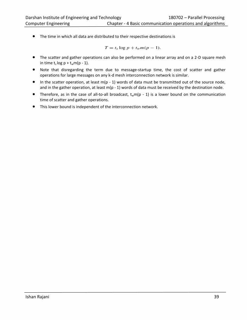
The time in which all data are distributed to their respective destinations is
The scatter and gather operations can also be performed on a linear array and on a 2-D square mesh
in time ts log p + twm(p - 1).
Note that disregarding the term due to message-startup time, the cost of scatter and gather
operations for large messages on any k-d mesh interconnection network is similar.
In the scatter operation, at least m(p - 1) words of data must be transmitted out of the source node,
and in the gather operation, at least m(p - 1) words of data must be received by the destination node.
Therefore, as in the case of all-to-all broadcast, twm(p - 1) is a lower bound on the communication
time of scatter and gather operations.
This lower bound is independent of the interconnection network.
Darshan Institute of Engineering and Technology 180702 - Parallel Processing
Computer Engineering Chapter – 5 Analytical Modelling of Parallel Platforms
Ishan Rajani 40
1) Enlist various performance metrics for parallel systems. Explain Speedup, Efficiency and total parallel
Overhead in brief. [June 13(7 marks), Oct. 12(7 marks), June 12(7 marks)]
A number of metrics have been used based on the desired outcome of performance analysis.
1. Execution Time:
The serial runtime of a program is the time elapsed between the beginning and the end of its
execution on a sequential computer.
The parallel runtime is the time that elapses from the moment a parallel computation starts to the
moment the last processing element finishes execution.
We denote the serial runtime by TS and the parallel runtime by TP.
2. Total Parallel Overhead:
The overheads incurred by a parallel program are encapsulated into a single expression referred to as
the overhead function.
We define overhead function or total overhead of a parallel system as the total time collectively
spent by all the processing elements over and above that required by the fastest known sequential
algorithm for solving the same problem on a single processing element.
We denote the overhead function of a parallel system by the symbol To.
The total time spent in solving a problem summed over all processing elements is pTP .
TS units of this time are spent performing useful work, and the remainder is overhead.
Therefore, the overhead function (To) is given by
T0 = pTp - Ts
3. Speedup:
When evaluating a parallel system, we are often interested in knowing how much performance gain
is achieved by parallelizing a given application over a sequential implementation.
Speedup is a measure that captures the relative benefit of solving a problem in parallel.
It is defined as the ratio of the time taken to solve a problem on a single processing element to the
time required to solve the same problem on a parallel computer with p identical processing
elements.
We denote speedup by the symbol S.
Only an ideal parallel system containing p processing elements can deliver a speedup equal to p.
In practice, ideal behavior is not achieved because while executing a parallel algorithm, the
processing elements cannot devote 100% of their time to the computations of the algorithm
4. Efficiency
Efficiency is a measure of the fraction of time for which a processing element is usefully employed; it
is defined as the ratio of speedup to the number of processing elements.
In an ideal parallel system, speedup is equal to p and efficiency is equal to one.
In practice, speedup is less than p and efficiency is between zero and one, depending on the
effectiveness with which the processing elements are utilized.
We denote efficiency by the symbol E. Mathematically, it is given by
E = S / P
Darshan Institute of Engineering and Technology 180702 - Parallel Processing
Computer Engineering Chapter – 5 Analytical Modelling of Parallel Platforms
Ishan Rajani 41
2) Define Isoefficiency function and derive equation of it. [June 13(7 marks), June 12(7 marks)]
Parallel execution time can be expressed as a function of problem size, overhead function, and the
number of processing elements. We can write parallel runtime as:
The resulting expression for speedup is
Finally, we write the expression for efficiency as
In above equation of E, if the problem size is kept constant and p is increased, the efficiency
decreases because the total overhead To increases with p.
If W is increased keeping the number of processing elements fixed, then for scalable parallel systems,
the efficiency increases.
This is because To grows slower than Q(W) for a fixed p. For these parallel systems, efficiency can be
maintained at a desired value (between 0 and 1) for increasing p, provided W is also increased.
For different parallel systems, W must be increased at different rates with respect to p in order to
maintain a fixed efficiency.
For instance, in some cases, W might need to grow as an exponential function of p to keep the
efficiency from dropping as p increases.
Such parallel systems are poorly scalable. The reason is that on these parallel systems it is difficult to
obtain good speedups for a large number of processing elements unless the problem size is
enormous.
On the other hand, if W needs to grow only linearly with respect to p, then the parallel system is
highly scalable.
That is because it can easily deliver speedups proportional to the number of processing elements for
reasonable problem sizes.
For scalable parallel systems, efficiency can be maintained at a fixed value (between 0 and 1) if the
ratio To/W in Equation of E is maintained at a constant value.
For a desired value E of efficiency,
Darshan Institute of Engineering and Technology 180702 - Parallel Processing
Computer Engineering Chapter – 5 Analytical Modelling of Parallel Platforms
Ishan Rajani 42
Let K = E/(1 - E) be a constant depending on the efficiency to be maintained. Since To is a function of
W and p, Above equation of W can be rewritten as
In above equation the problem size W can usually be obtained as a function of p by algebraic
manipulations.
This function dictates the growth rate of W required to keep the efficiency fixed as p increases. We
call this function the isoefficiency function of the parallel system.
The isoefficiency function determines the ease with which a parallel system can maintain a constant
efficiency and hence achieve speedups increasing in proportion to the number of processing
elements.
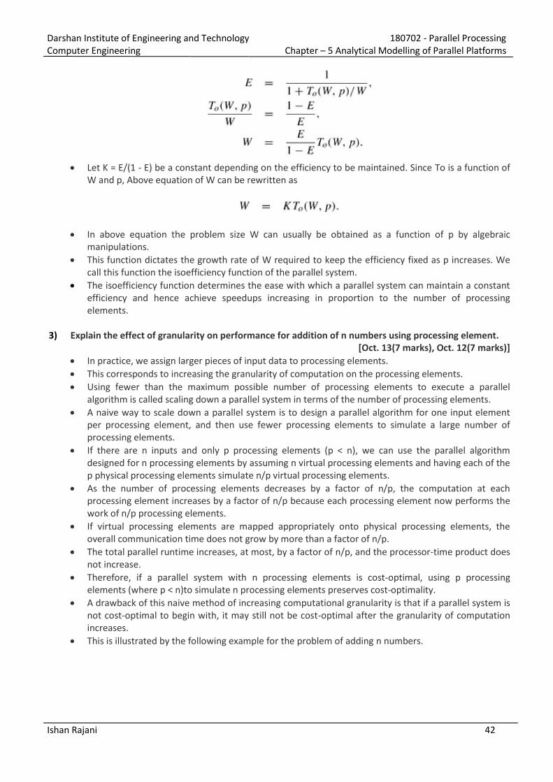
3) Explain the effect of granularity on performance for addition of n numbers using processing element.
[Oct. 13(7 marks), Oct. 12(7 marks)]
In practice, we assign larger pieces of input data to processing elements.
This corresponds to increasing the granularity of computation on the processing elements.
Using fewer than the maximum possible number of processing elements to execute a parallel
algorithm is called scaling down a parallel system in terms of the number of processing elements.
A naive way to scale down a parallel system is to design a parallel algorithm for one input element
per processing element, and then use fewer processing elements to simulate a large number of
processing elements.
If there are n inputs and only p processing elements (p < n), we can use the parallel algorithm
designed for n processing elements by assuming n virtual processing elements and having each of the
p physical processing elements simulate n/p virtual processing elements.
As the number of processing elements decreases by a factor of n/p, the computation at each
processing element increases by a factor of n/p because each processing element now performs the
work of n/p processing elements.
If virtual processing elements are mapped appropriately onto physical processing elements, the
overall communication time does not grow by more than a factor of n/p.
The total parallel runtime increases, at most, by a factor of n/p, and the processor-time product does
not increase.
Therefore, if a parallel system with n processing elements is cost-optimal, using p processing
elements (where p < n)to simulate n processing elements preserves cost-optimality.
A drawback of this naive method of increasing computational granularity is that if a parallel system is
not cost-optimal to begin with, it may still not be cost-optimal after the granularity of computation
increases.
This is illustrated by the following example for the problem of adding n numbers.
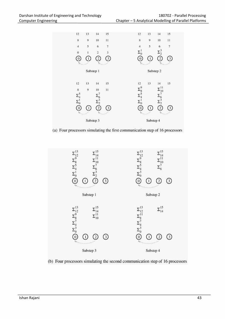
Darshan Institute of Engineering and Technology 180702 - Parallel Processing
Computer Engineering Chapter – 5 Analytical Modelling of Parallel Platforms
Ishan Rajani 43
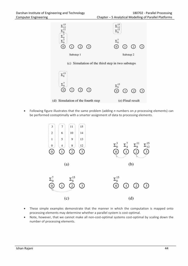
Darshan Institute of Engineering and Technology 180702 - Parallel Processing
Computer Engineering Chapter – 5 Analytical Modelling of Parallel Platforms
Ishan Rajani 44
Following figure illustrates that the same problem (adding n numbers on p processing elements) can
be performed costoptimally with a smarter assignment of data to processing elements.
These simple examples demonstrate that the manner in which the computation is mapped onto
processing elements may determine whether a parallel system is cost-optimal.
Note, however, that we cannot make all non-cost-optimal systems cost-optimal by scaling down the
number of processing elements.
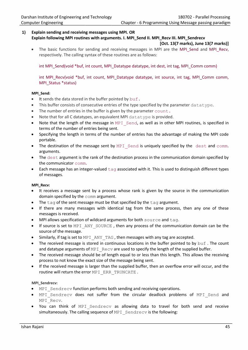
Darshan Institute of Engineering and Technology 180702 - Parallel Processing
Computer Engineering Chapter - 6 Programming Using Message passing paradigm
Ishan Rajani 45
1) Explain sending and receiving messages using MPI. OR
Explain following MPI routines with arguments. I. MPI_Send II. MPI_Recv III. MPI_Sendrecv
[Oct. 13(7 marks), June 13(7 marks)]
The basic functions for sending and receiving messages in MPI are the MPI_Send and MPI_Recv,
respectively. The calling syntax of these routines are as follows:
int MPI_Send(void *buf, int count, MPI_Datatype datatype, int dest, int tag, MPI_Comm comm)
int MPI_Recv(void *buf, int count, MPI_Datatype datatype, int source, int tag, MPI_Comm comm,
MPI_Status *status)
MPI_Send:
It sends the data stored in the buffer pointed by buf.
This buffer consists of consecutive entries of the type specified by the parameter datatype.
The number of entries in the buffer is given by the parameter count.
Note that for all C datatypes, an equivalent MPI datatype is provided.
Note that the length of the message in MPI_Send, as well as in other MPI routines, is specified in
terms of the number of entries being sent.
Specifying the length in terms of the number of entries has the advantage of making the MPI code
portable.
The destination of the message sent by MPI_Send is uniquely specified by the dest and comm.
arguments.
The dest argument is the rank of the destination process in the communication domain specified by
the communicator comm.
Each message has an integer-valued tag associated with it. This is used to distinguish different types
of messages.
MPI_Recv:
It receives a message sent by a process whose rank is given by the source in the communication
domain specified by the comm argument.
The tag of the sent message must be that specified by the tag argument.
If there are many messages with identical tag from the same process, then any one of these
messages is received.
MPI allows specification of wildcard arguments for both source and tag.
If source is set to MPI_ANY_SOURCE , then any process of the communication domain can be the
source of the message.
Similarly, if tag is set to MPI_ANY_TAG , then messages with any tag are accepted.
The received message is stored in continuous locations in the buffer pointed to by buf . The count
and datatype arguments of MPI_Recv are used to specify the length of the supplied buffer.
The received message should be of length equal to or less than this length. This allows the receiving
process to not know the exact size of the message being sent.
If the received message is larger than the supplied buffer, then an overflow error will occur, and the
routine will return the error MPI_ERR_TRUNCATE .
MPI_Sendrecv:
MPI_Sendrecv function performs both sending and receiving operations.
MPI_Sendrecv does not suffer from the circular deadlock problems of MPI_Send and
MPI_Recv.
You can think of MPI_Sendrecv as allowing data to travel for both send and receive
simultaneously. The calling sequence of MPI_Sendrecv is the following:
Darshan Institute of Engineering and Technology 180702 - Parallel Processing
Computer Engineering Chapter - 6 Programming Using Message passing paradigm
Ishan Rajani 46
int MPI_Sendrecv(void *sendbuf, int sendcount, MPI_Datatype senddatatype,
int dest, int sendtag, void *recvbuf, int recvcount, MPI_Datatype
recvdatatype, int source, int recvtag, MPI_Comm comm, MPI_Status *status)
The arguments of MPI_Sendrecv are essentially the combination of the arguments of MPI_Send
and MPI_Recv.
The send and receive buffers must be disjoint, and the source and destination of the messages can be
the same or different.
The safe version of our earlier example using MPI_Sendrecv is as follows.
In many programs, the requirement for the send and receive buffers of MPI_Sendrecv be disjoint
may force us to use a temporary buffer.
This increases the amount of memory required by the program and also increases the overall run
time due to the extra copy.
This problem can be solved by using that MPI_Sendrecv_replace MPI function.
This function performs a blocking send and receives, but it uses a single buffer for both the send and
receives operation.
That is, the received data replaces the data that was sent out of the buffer.
2) Differentiate blocking and non-blocking message passing operations. OR
Explain the blocking message passing send and receive operation.
[Oct. 13(7 marks), June 12(7 marks)]
Interactions among process of parallel computer can be performed by sending and receiving
messages.
Prototype declaration for send and receive is as follows:
Send(void *send_buf, int n_elems, int destination)
Receive(void *recv_buf, int n_elems, int source)
*send_buf is the pointer to the buffer that contains data to be sent.
For Send, n_elems is the number of elements from buffer to be sent and destination is the identifier
of process which receives data.
*recv_buf is the pointer to the buffer that stores received data.
For Receive, n_elems is the number of elements from buffer to be received and source is the idenfier
of process which sends data.
Following example illustrates the how process sends a piece of data to another process.
P0 P1
a = 10;
send(&a, 1, 1);
a = 0;
receive(&a, 1, 0);
printf(“%d\n”,a);
In a ove code process p sends value of varia le a to process p . After sending value p immediately change the value of a to zero.
P1 receives value of a from p0 and then prints that value. P1 should receive 10 instead of 0.
Message passing platforms have additional hardware to support these operations such as DMA and
Network interface.
DMA and Network interface allows transfer of message from buffer memory to destination without
involvement of CPU.
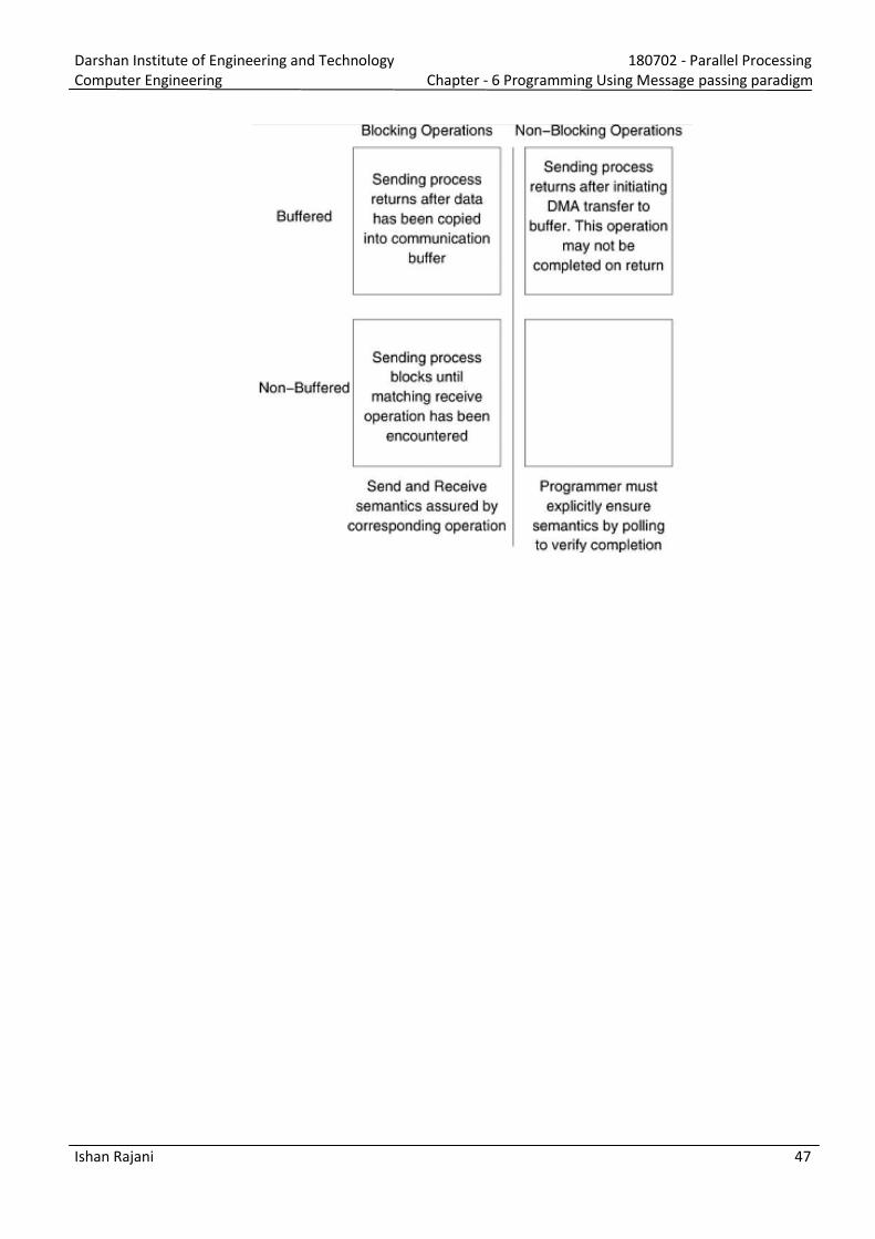
Darshan Institute of Engineering and Technology 180702 - Parallel Processing
Computer Engineering Chapter - 6 Programming Using Message passing paradigm
Ishan Rajani 47
Darshan Institute of Engineering and Technology 180702 - Parallel Processing
Computer Engineering Chapter - 7 Programming Shared Address Space Platforms
Ishan Rajani 48
1) Explain mutual exclusion for shared variable in Pthreads. OR
Explain three types of mutex normal, recursive and error check) in context to Pthread.
[Oct. 13(7 marks), June 13(7 marks)]
If multiple threads asks for same region at the same time then race condition occurs.
But various API provides utual exclusion locks also known as utex-lock for such shared data.
It has two states, locked and unlocked. The code that manipulate shared variable should have lock
associated with it.
Thread that tries to update value of that variable should first acquire the lock on that variable.
As only one lock on data is allowed at a time, no other thread can lock the same variable at the point
of that time and so process that tries to lock already locked variables is blocked.
Before leaving critical region value of locked variable should unlock.
So other thread can update its value.
At initial level all mutex locks are in unlocked state.
Pthread API provides two functions to lock or unlock shared variables as follows:
int pthread_mutex_lock(pthread_mutex_t *mutex_lock); int pthread_mutex_unlock(pthread_mutex_t *mutex_lock);
If thread successfully locked some variable then it enters into critical section.
If more than one blocked thread, then any one of them is allowd to enter in critical section based on
scheduling policy.
If any thread attempts to unlock the mutex that is already unlocked or which is locked by other
thread then no effect is defined.
Before using mutex, it should be initialized to unlock state by function pthread_mutex_init() as
follows:
int pthread_mutex_init(pthread_mutex_t *mutex_lock, const pthread_mutexattrtype *lock_attr);
It is possible to reduce locking by another lock function which is called pthread_mutex_trylock().
int pthread_mutex_trylock(pthread_mutex_t *mutex_lock);
If successfully locked it returns 0, otherwise it give that it is in busy state.
Types of mutex:
1. Normal:
It is default type locking.
Only single thread is allowed to lock normal mutex once at any point in time.
If thread with a lock attempts to lock it again, the second locking call results in deadlock.
PTHREAD_MUTEX_NORMAL_NP
2. Recursive:
It allows a single thread to lock mutex more than one time.
Each time thread lock the mutex, a lock counter is incremented. Each unlock decrements the counter.
Before another thread can lock an instance of this type of mutex, the locking thread must call the
pthread_mutex_unlock() routine the same number of time that it called the pthread_mutex_unlock()
routine the same number of times that it called the pthread_mutex_lock() routine.
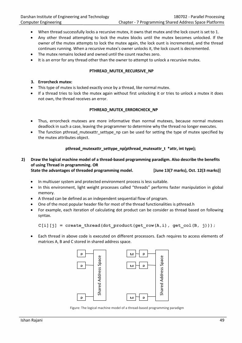
Darshan Institute of Engineering and Technology 180702 - Parallel Processing
Computer Engineering Chapter - 7 Programming Shared Address Space Platforms
Ishan Rajani 49
When thread successfully locks a recursive mutex, it owns that mutex and the lock count is set to 1.
Any other thread attempting to lock the mutex blocks until the mutex becomes unlocked. If the
owner of the mutex attempts to lock the mutex again, the lock ount is incremented, and the thread
continues running. When a recursive utex’s owner unlocks it, the lock count is decremented.
The mutex remains locked and owned until the count reaches zero.
It is an error for any thread other than the owner to attempt to unlock a recursive mutex.
PTHREAD_MUTEX_RECURSIVE_NP
3. Errorcheck mutex:
This type of mutex is locked exactly once by a thread, like normal mutex.
If a thread tries to lock the mutex again without first unlocking it or tries to unlock a mutex it does
not own, the thread receives an error.
PTHREAD_MUTEX_ERRORCHECK_NP
Thus, errorcheck mutexes are more informative than normal mutexes, because normal mutexes
deadlock in such a case, leaving the programmer to determine why the thread no longer executes.
The function pthread_mutexattr_settype_np can be used for setting the type of mutex specified by
the mutex attributes object.
pthread_mutexattr_settype_np(pthread_mutexattr_t *attr, int type);
2) Draw the logical machine model of a thread-based programming paradigm. Also describe the benefits
of using Thread in programming. OR
State the advantages of threaded programming model. [June 13(7 marks), Oct. 12(3 marks)]
In multiuser system and protected environment process is less suitable.
In this environ ent, light weight processes called threads perfor s faster anipulation in global
memory.
A thread can be defined as an independent sequential flow of program.
One of the most popular header file for most of the thread functionalities is pthread.h
For example, each iteration of calculating dot product can be consider as thread based on following
syntax.
C[i][j] = create_thread(dot_product(get_row(A,i), get_col(B, j)));
Each thread in above code is executed on different processors. Each requires to access elements of
matrices A, B and C stored in shared address space.
Figure: The logical machine model of a thread-based programming paradigm
P
P
P
Sh
are
d A
dd
ress
Sp
ace
P
P
P
Sh
are
d A
dd
ress
Sp
ace
M
M
M
Darshan Institute of Engineering and Technology 180702 - Parallel Processing
Computer Engineering Chapter - 7 Programming Shared Address Space Platforms
Ishan Rajani 50
As thread are executed as small functions, local variable of threads are treated as global data and are
stored in memory blocks M as shown in above figure.
As locality of data is important to improve performance, processes use cache memory to store local
variables.
Now we discuss about some of advantages and disadvantages as compared to messages passing
paradigm with regards to following criteria.
Thread creation:
int pthread_create(pthread)t *thread_id, const pthread_attr_t *attr, void * (*start_function) (void *), void *arg);
Thread join:
int pthread_join(pthread_t thread_id, void **ptr);
Thread Termination:
int pthread_exit(void *value_ptr);
Major Advantages of Thread based programming:
1. Software portability:
It means migration from serial to parallel programming
2. Scheduling/ Load Balancing:
Threaded programming provides large number of concurrent tasks which can be scheduled
explicitly.
Large number of concurrent tasks is mapped to multiple processors by dynamic mapping
techniques to reduce overheads of communication and idling.
3. Latency hiding:
When one thread is suffering from latency of memory other ready thread can execute its task by
using CPU.
4. Ease of programming:
It supports POSIX thread API which is the development tool for threaded programs. With the use of
this tool programming with thread becomes very easy.
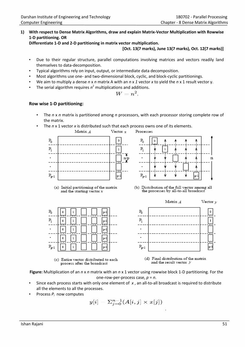
Darshan Institute of Engineering and Technology 180702 - Parallel Processing
Computer Engineering Chapter - 8 Dense Matrix Algorithms
Ishan Rajani 51
1) With respect to Dense Matrix Algorithms, draw and explain Matrix-Vector Multiplication with Rowwise
1-D partitioning. OR
Differentiate 1-D and 2-D partitioning in matrix vector multiplication.
[Oct. 13(7 marks), June 13(7 marks), Oct. 12(7 marks)]
• Due to their regular structure, parallel computations involving matrices and vectors readily land
themselves to data-decomposition.
• Typical algorithms rely on input, output, or intermediate data decomposition.
• Most algorithms use one- and two-dimensional block, cyclic, and block-cyclic partitionings.
• We aim to multiply a dense n x n matrix A with an n x 1 vector x to yield the n x 1 result vector y.
• The serial algorithm requires n2 multiplications and additions.
Row wise 1-D partitioning:
• The n x n matrix is partitioned among n processors, with each processor storing complete row of
the matrix.
• The n x 1 vector x is distributed such that each process owns one of its elements.
Figure: Multiplication of an n x n matrix with an n x 1 vector using rowwise block 1-D partitioning. For the
one-row-per-process case, p = n.
• Since each process starts with only one element of x , an all-to-all broadcast is required to distribute
all the elements to all the processes.
• Process Pi now computes
.
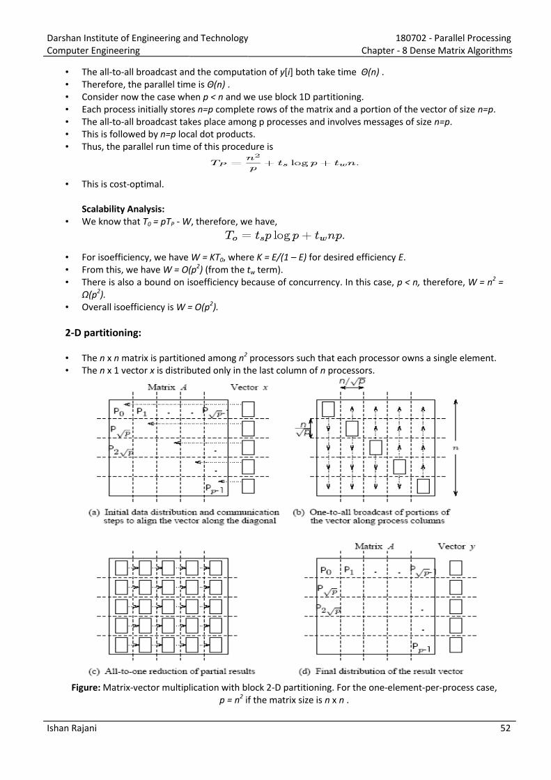
Darshan Institute of Engineering and Technology 180702 - Parallel Processing
Computer Engineering Chapter - 8 Dense Matrix Algorithms
Ishan Rajani 52
• The all-to-all broadcast and the computation of y[i] both take time Θ(n) .
• Therefore, the parallel time is Θ(n) .
• Consider now the case when p < n and we use block 1D partitioning.
• Each process initially stores n=p complete rows of the matrix and a portion of the vector of size n=p.
• The all-to-all broadcast takes place among p processes and involves messages of size n=p.
• This is followed by n=p local dot products.
• Thus, the parallel run time of this procedure is
• This is cost-optimal.
Scalability Analysis:
• We know that T0 = pTP - W, therefore, we have,
• For isoefficiency, we have W = KT0, where K = E/(1 – E) for desired efficiency E.
• From this, we have W = O(p2) (from the tw term).
• There is also a bound on isoefficiency because of concurrency. In this case, p < n, therefore, W = n2 =
Ω(p2).
• Overall isoefficiency is W = O(p2).
2-D partitioning:
• The n x n matrix is partitioned among n2 processors such that each processor owns a single element.
• The n x 1 vector x is distributed only in the last column of n processors.
Figure: Matrix-vector multiplication with block 2-D partitioning. For the one-element-per-process case,
p = n2 if the matrix size is n x n .
Darshan Institute of Engineering and Technology 180702 - Parallel Processing
Computer Engineering Chapter - 8 Dense Matrix Algorithms
Ishan Rajani 53
• We must first align the vector with the matrix appropriately.
• The first communication step for the 2-D partitioning aligns the vector x along the principal diagonal
of the matrix.
• The second step copies the vector elements from each diagonal process to all the processes in the
corresponding column using n simultaneous broadcasts among all processors in the column.
• Finally, the result vector is computed by performing an all-to-one reduction along the columns.
• Three basic communication operations are used in this algorithm: one-to-one communication to align
the vector along the main diagonal, one-to-all broadcast of each vector element among the n
processes of each column, and all-to-one reduction in each row.
• Each of these operations takes Θ(log n) time and the parallel time is Θ(log n) .
• The cost (process-time product) is Θ(n2 log n) ; hence, the algorithm is not cost-optimal.
• When using fewer than n2 processors, each process owns an (n/ � ) x (n/ � ) block of the matrix.
• The vector is distributed in portions of n/ � elements in the last process-column only.
• In this case, the message sizes for the alignment, broadcast, and reduction are all n/ �.
• The computation is a product of an (n/ � ) x (n/ � ) submatrix with a vector of length n/ �.
• The first alignment step takes time
• The broadcast and reductions take time
• Local matrix-vector products take time
• Total time is
Scalability Analysis:
• Equating T0 with W, term by term, for isoefficiency, we have W as the dominant term,
• The isoefficiency due to concurrency is O(p).
• The overall isoefficiency is (due to the network bandwidth).
• For cost optimality, we have,
Here p is,
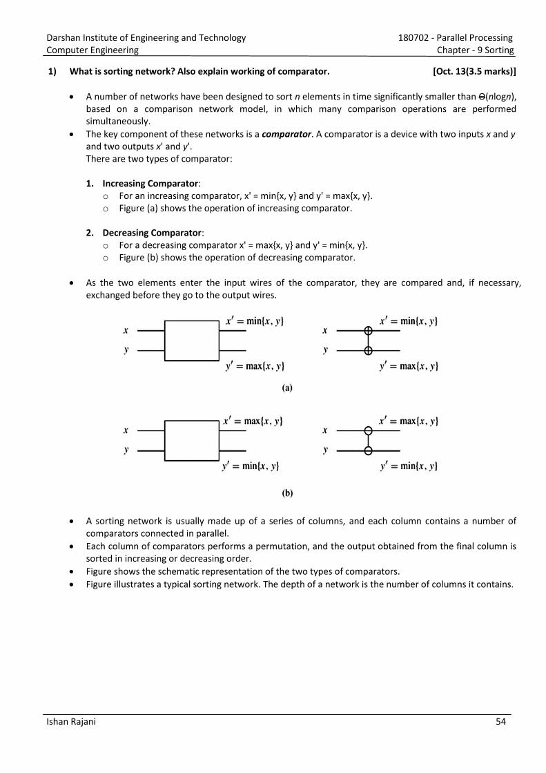
Darshan Institute of Engineering and Technology 180702 - Parallel Processing
Computer Engineering Chapter - 9 Sorting
Ishan Rajani 54
1) What is sorting network? Also explain working of comparator. [Oct. 13(3.5 marks)]
A number of networks have been designed to sort n elements in time significantly smaller than Ѳ(nlogn),
based on a comparison network model, in which many comparison operations are performed
simultaneously.
The key component of these networks is a comparator. A comparator is a device with two inputs x and y
and two outputs x' and y'.
There are two types of comparator:
1. Increasing Comparator:
o For an increasing comparator, x' = min{x, y} and y' = max{x, y}.
o Figure (a) shows the operation of increasing comparator.
2. Decreasing Comparator:
o For a decreasing comparator x' = max{x, y} and y' = min{x, y}.
o Figure (b) shows the operation of decreasing comparator.
As the two elements enter the input wires of the comparator, they are compared and, if necessary,
exchanged before they go to the output wires.
A sorting network is usually made up of a series of columns, and each column contains a number of
comparators connected in parallel.
Each column of comparators performs a permutation, and the output obtained from the final column is
sorted in increasing or decreasing order.
Figure shows the schematic representation of the two types of comparators.
Figure illustrates a typical sorting network. The depth of a network is the number of columns it contains.
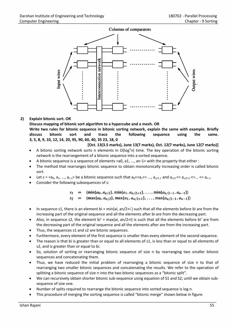
Darshan Institute of Engineering and Technology 180702 - Parallel Processing
Computer Engineering Chapter - 9 Sorting
Ishan Rajani 55
2) Explain bitonic sort. OR
Discuss mapping of bitonic sort algorithm to a hypercube and a mesh. OR
Write two rules for bitonic sequence in bitonic sorting network, explain the same with example. Briefly
discuss bitonic sort and trace the following sequence using the same.
3, 5, 8, 9, 10, 12, 14, 20, 95, 90, 60, 40, 35 23, 18, 0
[Oct. 13(3.5 marks), June 13(7 marks), Oct. 12(7 marks), June 12(7 marks)]
A bitonic sorting network sorts n elements in O(log2n) time. The key operation of the bitonic sorting
network is the rearrangement of a bitonic sequence into a sorted sequence.
A bitonic sequence is a sequence of elements <a0, a1, ..., an-1> with the property that either :
The method that rearranges bitonic sequence to obtain monotonically increasing order is called bitonic
sort.
Let s = <a0, a1, ..., an-1> be a bitonic sequence such that a0<=a1<= ..., an/2-1 and an/2 <= an/2+1 <=... <= an-1.
Consider the following subsequences of s:
In sequence s1, there is an element bi = min{ai, an/2+i } such that all the elements before bi are from the
increasing part of the original sequence and all the elements after bi are from the decreasing part.
Also, in se uence s2, the ele ent i’ = ax{ai, an/2+i} is such that all the ele ents efore i’ are fro the decreasing part of the original sequence and all the elements after are from the increasing part.
Thus, the sequences s1 and s2 are bitonic sequences.
Furthermore, every element of the first sequence is smaller than every element of the second sequence.
The reason is that bi is greater than or equal to all elements of s1, is less than or equal to all elements of
s2, and is greater than or equal to bi.
So, solution of sorting or rearranging bitonic sequence of size n by rearranging two smaller bitonic
sequences and concatenating them.
Thus, we have reduced the initial problem of rearranging a bitonic sequence of size n to that of
rearranging two smaller bitonic sequences and concatenating the results. We refer to the operation of
splitting a itonic se uence of size n into the two itonic se uences as a itonic split . We can recursively obtain shorter bitonic sub-sequence using equation of S1 and S2; until we obtain sub-
sequence of size one.
Number of splits required to rearrange the bitonic sequence into sorted sequence is log n.
This procedure of erging the sorting se uence is called itonic erge shown elow in figure.
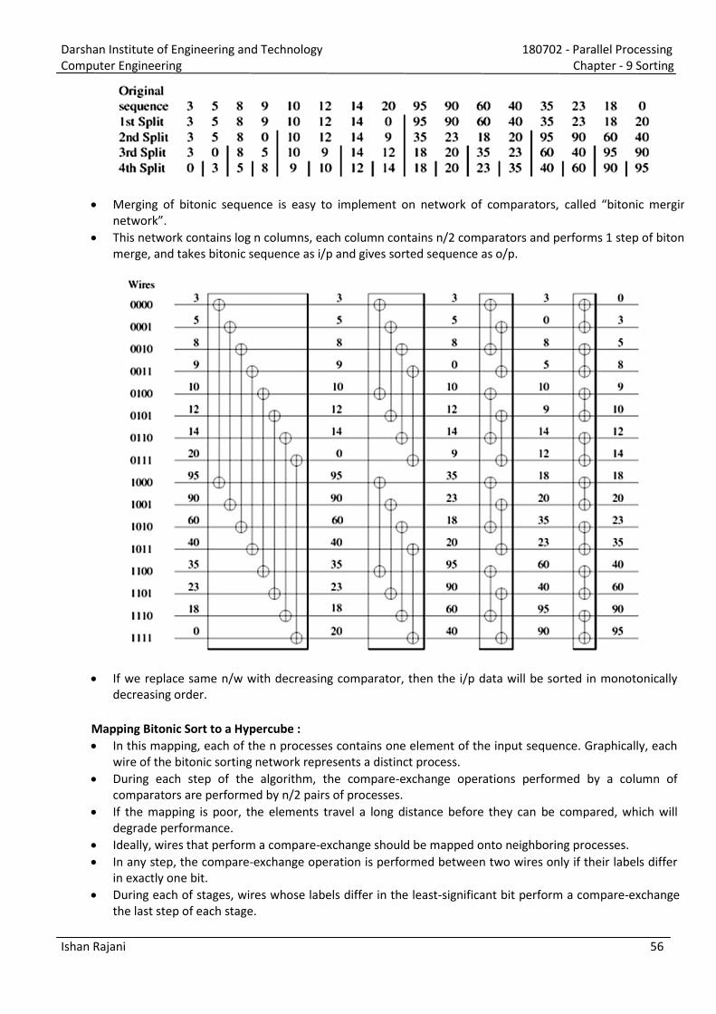
Darshan Institute of Engineering and Technology 180702 - Parallel Processing
Computer Engineering Chapter - 9 Sorting
Ishan Rajani 56
Merging of bitonic sequence is easy to implement on network of comparators, called itonic erging
network . This network contains log n columns, each column contains n/2 comparators and performs 1 step of bitonic
merge, and takes bitonic sequence as i/p and gives sorted sequence as o/p.
If we replace same n/w with decreasing comparator, then the i/p data will be sorted in monotonically
decreasing order.
Mapping Bitonic Sort to a Hypercube :
In this mapping, each of the n processes contains one element of the input sequence. Graphically, each
wire of the bitonic sorting network represents a distinct process.
During each step of the algorithm, the compare-exchange operations performed by a column of
comparators are performed by n/2 pairs of processes.
If the mapping is poor, the elements travel a long distance before they can be compared, which will
degrade performance.
Ideally, wires that perform a compare-exchange should be mapped onto neighboring processes.
In any step, the compare-exchange operation is performed between two wires only if their labels differ
in exactly one bit.
During each of stages, wires whose labels differ in the least-significant bit perform a compare-exchange in
the last step of each stage.
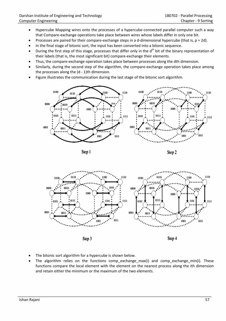
Darshan Institute of Engineering and Technology 180702 - Parallel Processing
Computer Engineering Chapter - 9 Sorting
Ishan Rajani 57
Hypercube Mapping wires onto the processes of a hypercube-connected parallel computer such a way
that Compare-exchange operations take place between wires whose labels differ in only one bit.
Processes are paired for their compare-exchange steps in a d-dimensional hypercube (that is, p = 2d).
In the final stage of bitonic sort, the input has been converted into a bitonic sequence.
During the first step of this stage, processes that differ only in the dth
bit of the binary representation of
their labels (that is, the most significant bit) compare-exchange their elements.
Thus, the compare-exchange operation takes place between processes along the dth dimension.
Similarly, during the second step of the algorithm, the compare-exchange operation takes place among
the processes along the (d - 1)th dimension.
Figure illustrates the communication during the last stage of the bitonic sort algorithm.
The bitonic sort algorithm for a hypercube is shown below.
The algorithm relies on the functions comp_exchange_max(i) and comp_exchange_min(i). These
functions compare the local element with the element on the nearest process along the ith dimension
and retain either the minimum or the maximum of the two elements.
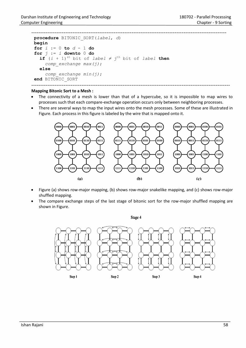
Darshan Institute of Engineering and Technology 180702 - Parallel Processing
Computer Engineering Chapter - 9 Sorting
Ishan Rajani 58
------------------------------------------------------------------------------------------------------------- procedure BITONIC_SORT(label, d) begin for i := 0 to d - 1 do for j := i downto 0 do if (i + 1)st bit of label ≠ jth bit of label then comp_exchange max(j); else comp_exchange min(j); end BITONIC_SORT
--------------------------------------------------------------------------------------------------------------- Mapping Bitonic Sort to a Mesh :
The connectivity of a mesh is lower than that of a hypercube, so it is impossible to map wires to
processes such that each compare-exchange operation occurs only between neighboring processes.
There are several ways to map the input wires onto the mesh processes. Some of these are illustrated in
Figure. Each process in this figure is labeled by the wire that is mapped onto it.
Figure (a) shows row-major mapping, (b) shows row-major snakelike mapping, and (c) shows row-major
shuffled mapping.
The compare exchange steps of the last stage of bitonic sort for the row-major shuffled mapping are
shown in Figure.
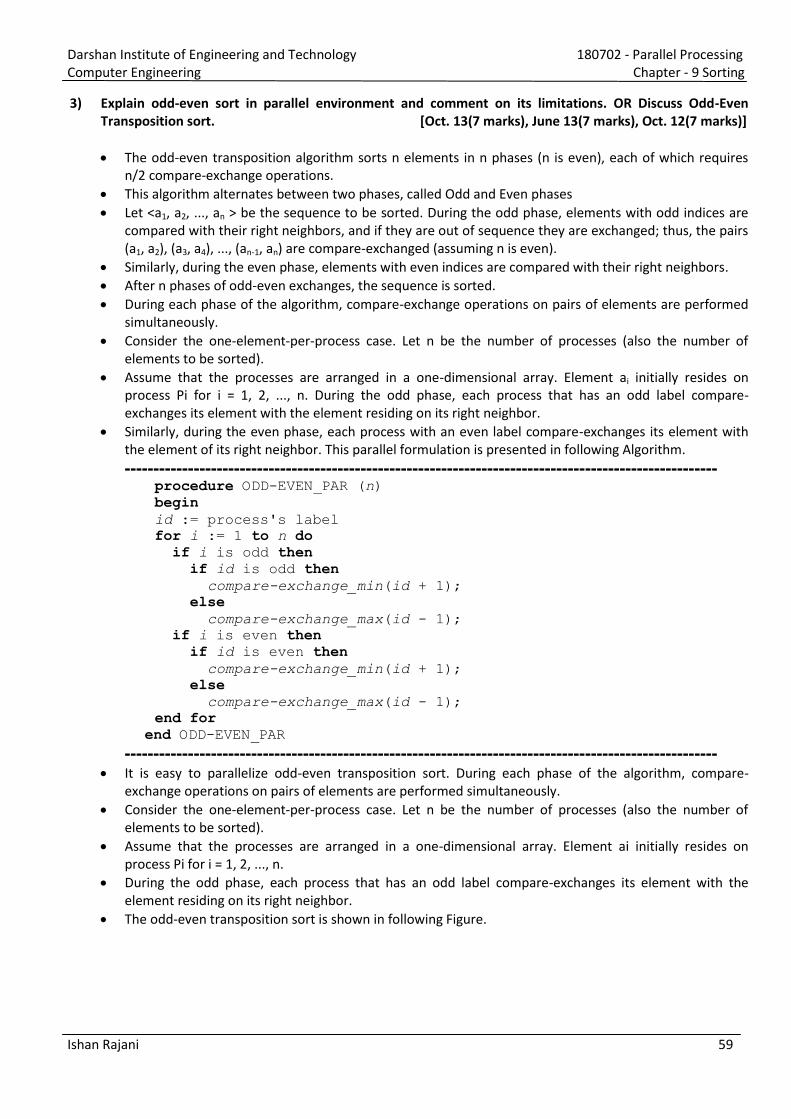
Darshan Institute of Engineering and Technology 180702 - Parallel Processing
Computer Engineering Chapter - 9 Sorting
Ishan Rajani 59
3) Explain odd-even sort in parallel environment and comment on its limitations. OR Discuss Odd-Even
Transposition sort. [Oct. 13(7 marks), June 13(7 marks), Oct. 12(7 marks)]
The odd-even transposition algorithm sorts n elements in n phases (n is even), each of which requires
n/2 compare-exchange operations.
This algorithm alternates between two phases, called Odd and Even phases
Let <a1, a2, ..., an > be the sequence to be sorted. During the odd phase, elements with odd indices are
compared with their right neighbors, and if they are out of sequence they are exchanged; thus, the pairs
(a1, a2), (a3, a4), ..., (an-1, an) are compare-exchanged (assuming n is even).
Similarly, during the even phase, elements with even indices are compared with their right neighbors.
After n phases of odd-even exchanges, the sequence is sorted.
During each phase of the algorithm, compare-exchange operations on pairs of elements are performed
simultaneously.
Consider the one-element-per-process case. Let n be the number of processes (also the number of
elements to be sorted).
Assume that the processes are arranged in a one-dimensional array. Element ai initially resides on
process Pi for i = 1, 2, ..., n. During the odd phase, each process that has an odd label compare-
exchanges its element with the element residing on its right neighbor.
Similarly, during the even phase, each process with an even label compare-exchanges its element with
the element of its right neighbor. This parallel formulation is presented in following Algorithm.
------------------------------------------------------------------------------------------------------- procedure ODD-EVEN_PAR (n) begin id := process's label for i := 1 to n do if i is odd then if id is odd then compare-exchange_min(id + 1); else compare-exchange_max(id - 1); if i is even then if id is even then compare-exchange_min(id + 1); else compare-exchange_max(id - 1); end for
end ODD-EVEN_PAR
------------------------------------------------------------------------------------------------------- It is easy to parallelize odd-even transposition sort. During each phase of the algorithm, compare-
exchange operations on pairs of elements are performed simultaneously.
Consider the one-element-per-process case. Let n be the number of processes (also the number of
elements to be sorted).
Assume that the processes are arranged in a one-dimensional array. Element ai initially resides on
process Pi for i = 1, 2, ..., n.
During the odd phase, each process that has an odd label compare-exchanges its element with the
element residing on its right neighbor.
The odd-even transposition sort is shown in following Figure.
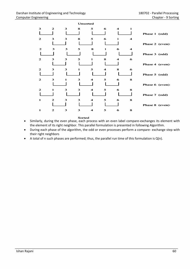
Darshan Institute of Engineering and Technology 180702 - Parallel Processing
Computer Engineering Chapter - 9 Sorting
Ishan Rajani 60
Similarly, during the even phase, each process with an even label compare-exchanges its element with
the element of its right neighbor. This parallel formulation is presented in following Algorithm.
During each phase of the algorithm, the odd or even processes perform a compare- exchange step with
their right neighbors
A total of n such phases are performed; thus, the parallel run time of this formulation is Q(n).
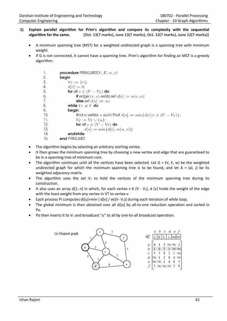
Darshan Institute of Engineering and Technology 180702 - Parallel Processing
Computer Engineering Chapter - 10 Graph Algorithms
Ishan Rajani 61
1) E plai pa allel algo ith fo P i ’s algo ith a d co pa e its co ple it with the se ue tial algorithm for the same. [Oct. 13(7 marks), June 13(7 marks), Oct. 12(7 marks), June 12(7 marks)]
A minimum spanning tree (MST) for a weighted undirected graph is a spanning tree with minimum
weight.
If G is not connected, it cannot have a spanning tree. Prim's algorithm for finding an MST is a greedy
algorithm.
The algorithm begins by selecting an arbitrary starting vertex.
It then grows the minimum spanning tree by choosing a new vertex and edge that are guaranteed to
be in a spanning tree of minimum cost.
The algorithm continues until all the vertices have been selected. Let G = (V, E, w) be the weighted
undirected graph for which the minimum spanning tree is to be found, and let A = (ai, j) be its
weighted adjacency matrix.
The algorithm uses the set VT to hold the vertices of the minimum spanning tree during its
construction.
It also uses an array d[1..n] in which, for each vertex v € (V - VT), d [v] holds the weight of the edge
with the least weight from any vertex in VT to vertex v.
Each process Pi computes di[u]=min { d[v] / vє(V- VT)} during each iteration of while loop.
The global minimum is then obtained over all di[u] by all-to-one reduction operation and sorted in
Po.
Po then inserts it to VT and roadcast u to all y one-to-all broadcast operation.
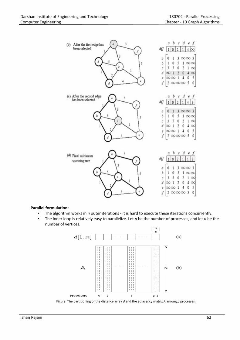
Darshan Institute of Engineering and Technology 180702 - Parallel Processing
Computer Engineering Chapter - 10 Graph Algorithms
Ishan Rajani 62
Parallel formulation:
• The algorithm works in n outer iterations - it is hard to execute these iterations concurrently.
• The inner loop is relatively easy to parallelize. Let p be the number of processes, and let n be the
number of vertices.
Figure: The partitioning of the distance array d and the adjacency matrix A among p processes.
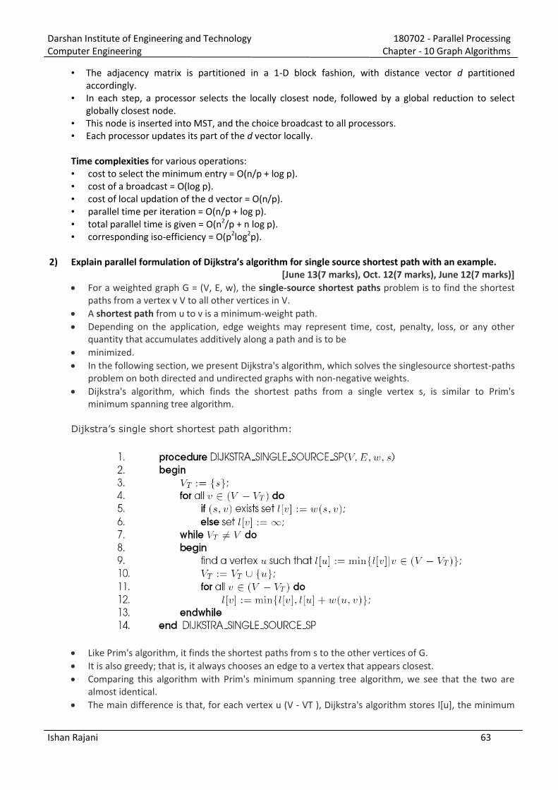
Darshan Institute of Engineering and Technology 180702 - Parallel Processing
Computer Engineering Chapter - 10 Graph Algorithms
Ishan Rajani 63
• The adjacency matrix is partitioned in a 1-D block fashion, with distance vector d partitioned
accordingly.
• In each step, a processor selects the locally closest node, followed by a global reduction to select
globally closest node.
• This node is inserted into MST, and the choice broadcast to all processors.
• Each processor updates its part of the d vector locally.
Time complexities for various operations:
• cost to select the minimum entry = O(n/p + log p).
• cost of a broadcast = O(log p).
• cost of local updation of the d vector = O(n/p).
• parallel time per iteration = O(n/p + log p).
• total parallel time is given = O(n2/p + n log p).
• corresponding iso-efficiency = O(p2log
2p).
2) Explain parallel fo ulatio of Dijkst a’s algo ith fo si gle sou ce sho test path with a e a ple. [June 13(7 marks), Oct. 12(7 marks), June 12(7 marks)]
For a weighted graph G = (V, E, w), the single-source shortest paths problem is to find the shortest
paths from a vertex v V to all other vertices in V.
A shortest path from u to v is a minimum-weight path.
Depending on the application, edge weights may represent time, cost, penalty, loss, or any other
quantity that accumulates additively along a path and is to be
minimized.
In the following section, we present Dijkstra's algorithm, which solves the singlesource shortest-paths
problem on both directed and undirected graphs with non-negative weights.
Dijkstra's algorithm, which finds the shortest paths from a single vertex s, is similar to Prim's
minimum spanning tree algorithm.
Dijkstra’s single short shortest path algorithm:
Like Prim's algorithm, it finds the shortest paths from s to the other vertices of G.
It is also greedy; that is, it always chooses an edge to a vertex that appears closest.
Comparing this algorithm with Prim's minimum spanning tree algorithm, we see that the two are
almost identical.
The main difference is that, for each vertex u (V - VT ), Dijkstra's algorithm stores l[u], the minimum
Darshan Institute of Engineering and Technology 180702 - Parallel Processing
Computer Engineering Chapter - 10 Graph Algorithms
Ishan Rajani 64
cost to reach vertex u from vertex s by means of vertices in VT; Prim's algorithm stores d [u], the cost
of the minimum-cost edge connecting a vertex in VT to u. The run time of Dijkstra's algorithm is
Ѳ(n2).
Parallel Formulation:
The parallel formulation of Dijkstra's single-source shortest path algorithm is very similar to the
parallel formulation of Prim's algorithm for minimum spanning trees. The weighted adjacency matrix
is partitioned using the 1-D block mapping.
Each of the p processes is assigned n/p consecutive columns of the weighted adjacency matrix, and
computes n/p values of the array l.
During each iteration, all processes perform computation and communication similar to that
performed by the parallel formulation of Prim's algorithm.
Consequently, the parallel performance and scalability of Dijkstra's single-source shortest path
algorithm is identical to that of Prim's minimum spanning tree algorithm.
Related Documents