Faculty of Actuaries Institute of Actuaries EXAMINATION 13 April 2005 (am) Subject CT4 (103) Models (103 Part) Core Technical Time allowed: One and a half hours INSTRUCTIONS TO THE CANDIDATE 1. Enter all the candidate and examination details as requested on the front of your answer booklet. 2. You must not start writing your answers in the booklet until instructed to do so by the supervisor. 3. Mark allocations are shown in brackets. 4. Attempt all 6 questions, beginning your answer to each question on a separate sheet. 5. Candidates should show calculations where this is appropriate. Graph paper is not required for this paper. AT THE END OF THE EXAMINATION Hand in BOTH your answer booklet, with any additional sheets firmly attached, and this question paper. In addition to this paper you should have available the 2002 edition of the Formulae and Tables and your own electronic calculator. Faculty of Actuaries CT4 (103) A2005 Institute of Actuaries

Welcome message from author
This document is posted to help you gain knowledge. Please leave a comment to let me know what you think about it! Share it to your friends and learn new things together.
Transcript

Faculty of Actuaries Institute of Actuaries
EXAMINATION
13 April 2005 (am)
Subject CT4 (103)
Models (103 Part) Core Technical
Time allowed: One and a half hours
INSTRUCTIONS TO THE CANDIDATE
1. Enter all the candidate and examination details as requested on the front of your answer booklet.
2. You must not start writing your answers in the booklet until instructed to do so by the supervisor.
3. Mark allocations are shown in brackets.
4. Attempt all 6 questions, beginning your answer to each question on a separate sheet.
5. Candidates should show calculations where this is appropriate.
Graph paper is not required for this paper.
AT THE END OF THE EXAMINATION
Hand in BOTH your answer booklet, with any additional sheets firmly attached, and this question paper.
In addition to this paper you should have available the 2002 edition of the Formulae and Tables and your own electronic calculator.
Faculty of Actuaries CT4 (103) A2005 Institute of Actuaries
CT4 (103) A2005 2
1 (i) Define each of the following examples of a stochastic process
(a) a symmetric simple random walk (b) a compound Poisson process
[2]
(ii) For each of the processes in (i), classify it as a stochastic process according to its state space and the time that it operates on. [2]
[Total 4]
2 You have been commissioned to develop a model to project the assets and liabilities of an insurer after one year. This has been requested following a change in the regulatory capital requirement. Sufficient capital must now be held such that there is less than a 0.5% chance of liabilities exceeding assets after one year.
The company does not have any existing stochastic models, but estimates have been made in the planning process of worst case scenarios.
Set out the steps you would take in the development of the model. [6]
3 Let Y1, Y3, Y5, , be a sequence of independent and identically distributed random variables with
2 1 2 11
= 1 = = 1 = , = 0, 1, 2,...2k kP Y P Y k
and define 2 2 1 2 1= /k k kY Y Y for k = 1, 2, .
(i) Show that : = 1, 2,...kY k is a sequence of independent and identically
distributed random variables.
Hint: You may use the fact that, if X, Y are two variables that take only two values and ( ),E XY E X E Y then X, Y are independent. [4]
(ii) Explain whether or not : = 1, 2,...kY k constitutes a Markov chain. [1]
(iii) (a) State the transition probabilities ( ) = = | =ij m n mp n P Y j Y i of the
sequence : = 1, 2,...kY k .
(b) Hence show that these probabilities do not depend on the current state and that they satisfy the Chapman-Kolmogorov equations.
[3] [Total 8]
CT4 (103) A2005 3 PLEASE TURN OVER
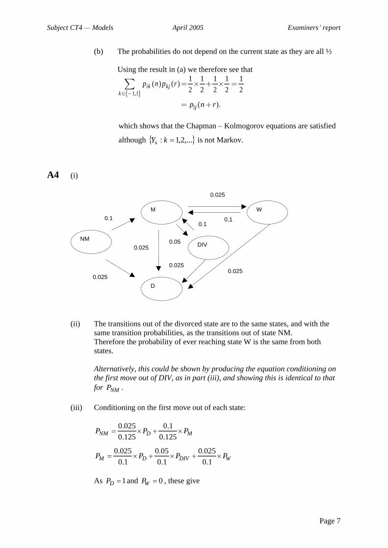
4 Marital status is considered using the following time-homogeneous, continuous time Markov jump process:
the transition rate from unmarried to married is 0.1 per annum
the divorce rate is equivalent to a transition rate of 0.05 per annum
the mortality rate for any individual is equivalent to a transition rate of 0.025 per annum, independent of marital status
The state space of the process consists of five states: Never Married (NM), Married (M), Widowed (W), Divorced (DIV) and Dead (D).
Px is the probability that a person currently in state x, and who has never previously been widowed, will die without ever being widowed.
(i) Construct a transition diagram between the five states. [2]
(ii) Show, by general reasoning or otherwise, that NMP equals DIVP . [1]
(iii) Demonstrate that:
1 4
5 51 1
4 2
NM M
M DIV
P P
P P
[2]
(iv) Calculate the probability of never being widowed if currently in state NM. [2]
(v) Suggest two ways in which the model could be made more realistic. [1] [Total 8]

CT4 (103) A2005 4
5 A No-Claims Discount system operated by a motor insurer has the following four levels:
Level 1: 0% discount Level 2: 25% discount Level 3: 40% discount Level 4: 60% discount
The rules for moving between these levels are as follows:
Following a year with no claims, move to the next higher level, or remain at level 4.
Following a year with one claim, move to the next lower level, or remain at level 1.
Following a year with two or more claims, move back two levels, or move to level 1 (from level 2) or remain at level 1.
For a given policyholder the probability of no claims in a given year is 0.85 and the probability of making one claim is 0.12.
X(t) denotes the level of the policyholder in year t.
(i) (a) Explain why X(t) is a Markov chain. (b) Write down the transition matrix of this chain.
[2]
(ii) Calculate the probability that a policyholder who is currently at level 2 will be at level 2 after:
(a) one year (b) two years (c) three years
[3]
(iii) Explain whether the chain is irreducible and/or aperiodic. [2]
(iv) Calculate the long-run probability that a policyholder is in discount level 2. [5]
[Total 12]
CT4(103) A2005 5
6 An insurance policy covers the repair of a washing machine, and is subject to a maximum of 3 claims over the year of coverage.
The probability of the machine breaking down has been estimated to follow an exponential distribution with the following annualised frequencies, :
1/10 If the machine has not suffered any previous breakdown.
= }
1/5 If the machine has broken down once previously. 1/4 If the machine has broken down on two or more occasions.
As soon as a breakdown occurs an engineer is despatched. It can be assumed that the repair is made immediately, and that it is always possible to repair the machine.
The washing machine has never broken down at the start of the year (time t = 0).
Pi(t) is the probability that the machine has suffered i breakdowns by time t.
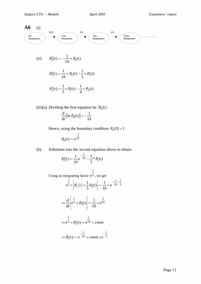
(i) Draw a transition diagram for the process defined by the number of breakdowns occurring up to time t. [1]
(ii) Write down the Kolmogorov equations obeyed by 0 1( ), ( )P t P t and 2( )P t . [2]
(iii) (a) Derive an expression for 0 ( )P t and
(b) demonstrate that 10 51( ) =
t t
P t e e . [3]
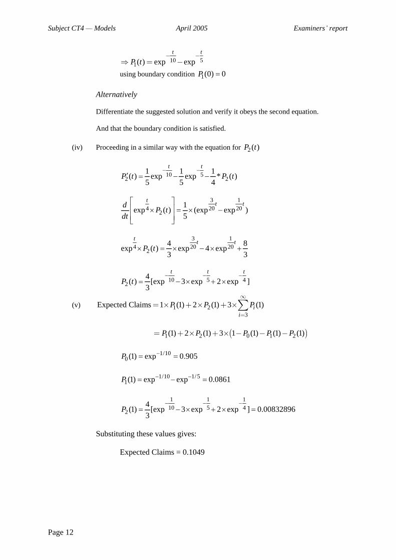
(iv) Derive an expression for 2( )P t . [3]
(v) Calculate the expected number of claims under the policy. [3] [Total 12]
END OF PAPER

Faculty of Actuaries Institute of Actuaries
EXAMINATION
13 April 2005 (am)
Subject CT4 (104)
Models (104 Part) Core Technical
Time allowed: One and a half hours
INSTRUCTIONS TO THE CANDIDATE
1. Enter all the candidate and examination details as requested on the front of your answer booklet.
2. You must not start writing your answers in the booklet until instructed to do so by the supervisor.
3. Mark allocations are shown in brackets.
4. Attempt all 7 questions, beginning your answer to each question on a separate sheet.
5. Candidates should show calculations where this is appropriate.
Graph paper is not required for this paper.
AT THE END OF THE EXAMINATION
Hand in BOTH your answer booklet, with any additional sheets firmly attached, and this question paper.
In addition to this paper you should have available the 2002 edition of the Formulae and Tables and your own electronic calculator.
Faculty of Actuaries CT4 (104) A2005 Institute of Actuaries
CT4 (104) A2005 2
1 (i) Write down the equation of the Cox proportional hazards model in which the hazard function depends on duration t and a vector of covariates z. You should define all the other terms that you use. [2]
(ii) Explain why the Cox model is sometimes described as semi-parametric . [1] [Total 3]
2 Show that if the force of mortality x t
(0 t 1) is given by
=1
xx t
x
q
tq,
this implies that deaths between exact ages x and x + 1 are uniformly distributed. [4]
3 An investigation of mortality over the whole age range produced crude estimates of qx
for exact ages x from 2 years to 93 years inclusive. The actual deaths at each age were compared with the number of deaths which would have been expected had the mortality of the lives in the investigation been the same as English Life Table 15 (ELT15). 53 of the deviations were positive and 39 were negative.
Test whether the underlying mortality of the lives in the investigation is represented by ELT15. [5]
4 A life insurance company has investigated the recent mortality experience of its male term assurance policy holders by estimating the mortality rate at each age, qx . It is proposed that the crude rates might be graduated by reference to a standard mortality
table for male permanent assurance policy holders with forces of mortality 12
s
x, so
that the forces of mortality 12
x implied by the graduated rates xq are given by the
function:
1 12 2
= s
x xk ,
where k is a constant.
(i) Describe how the suitability of the above function for graduating the crude rates could be investigated. [2]
(ii) (a) Explain how the constant k can be estimated by weighted least squares.
(b) Suggest suitable weights. [4]
(iii) Explain how the smoothness of the graduated rates is achieved. [1] [Total 7]
CT4 (104) A2005 3 PLEASE TURN OVER
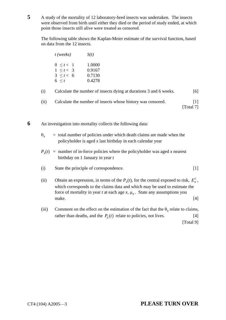
5 A study of the mortality of 12 laboratory-bred insects was undertaken. The insects were observed from birth until either they died or the period of study ended, at which point those insects still alive were treated as censored.
The following table shows the Kaplan-Meier estimate of the survival function, based on data from the 12 insects.
t (weeks) S(t)
0
t < 1 1.0000
1
t < 3 0.9167 3
t < 6 0.7130 6
t 0.4278
(i) Calculate the number of insects dying at durations 3 and 6 weeks. [6]
(ii) Calculate the number of insects whose history was censored. [1] [Total 7]
6 An investigation into mortality collects the following data:
x = total number of policies under which death claims are made when the policyholder is aged x last birthday in each calendar year
Px(t) = number of in-force policies where the policyholder was aged x nearest birthday on 1 January in year t
(i) State the principle of correspondence. [1]
(ii) Obtain an expression, in terms of the Px(t), for the central exposed to risk, cxE ,
which corresponds to the claims data and which may be used to estimate the force of mortality in year t at each age x, x . State any assumptions you make. [4]
(iii) Comment on the effect on the estimation of the fact that the x relate to claims,
rather than deaths, and the ( )xP t relate to policies, not lives. [4]
[Total 9]
CT4 (104) A2005 4
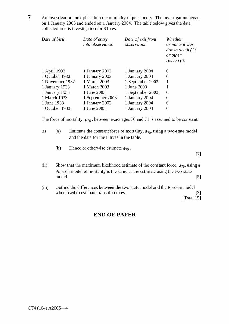
7 An investigation took place into the mortality of pensioners. The investigation began on 1 January 2003 and ended on 1 January 2004. The table below gives the data collected in this investigation for 8 lives.
Date of birth Date of entry Date of exit from Whether into observation observation or not exit was
due to death (1) or other reason (0)
1 April 1932 1 January 2003 1 January 2004 0 1 October 1932 1 January 2003 1 January 2004 0 1 November 1932 1 March 2003 1 September 2003 1 1 January 1933 1 March 2003 1 June 2003 1 1 January 1933 1 June 2003 1 September 2003 0 1 March 1933 1 September 2003 1 January 2004 0 1 June 1933 1 January 2003 1 January 2004 0 1 October 1933 1 June 2003 1 January 2004 0
The force of mortality, 70 , between exact ages 70 and 71 is assumed to be constant.
(i) (a) Estimate the constant force of mortality, 70, using a two-state model and the data for the 8 lives in the table.
(b) Hence or otherwise estimate q70 . [7]
(ii) Show that the maximum likelihood estimate of the constant force, 70, using a Poisson model of mortality is the same as the estimate using the two-state model. [5]
(iii) Outline the differences between the two-state model and the Poisson model when used to estimate transition rates. [3]
[Total 15]
END OF PAPER

Faculty of Actuaries Institute of Actuaries
EXAMINATION
April 2005
Subject CT4
Models (includes both 103 and 104 parts) Core Technical
EXAMINERS REPORT
Faculty of Actuaries Institute of Actuaries

Subject CT4 Models April 2005 Examiners report
Page 2
EXAMINERS COMMENTS
Comments on solutions presented to individual questions for this April 2005 paper are given below:
103 Part
Question A1 This was reasonably well answered. Descriptive (rather than formulaic) answers to part (i) were given equal credit. Very few candidates correctly identified the state space for the compound Poisson process in part (ii).
Question A2 This was reasonably well answered. Marks were lost by candidates who did not provide sufficient detail or did not provide enough distinct points. Some candidates attempted to define the model they would adopt, rather than the stages in the modelling process.
Question A3 This was very poorly attempted by most candidates. Very few candidates provided any real attempt at part (i). The examiners were looking here for a demonstration of pairwise (not mutual) independence, and the hint should have made this clear. In part (ii), most candidates wrongly stated that the sequence was Markov. Many candidates did not attempt part (iii); this may be because of the failure to make any progress in part (i), although it should be noted that subsequent parts of the question did not depend on correctly answering part (i).
Question A4 This was well answered overall. In part (i), some candidates did not allow for re-marriage from the divorced or widowed states, which then caused them problems in part (ii). Candidates lost marks in part (iii) if they did not provide sufficient explanation of their steps.
Question A5 This was very well answered, with the majority of candidates scoring highly.
Question A6 Overall this was not well answered, but the better candidates did score well. Many candidates produced good answers to part (i) to (iv). In part (iii), a number of candidates did not verify that the boundary conditions were satisfied. Some candidates struggled with part (v) and a significant number did not attempt this part of the question.

Subject CT4 Models April 2005 Examiners report
Page 3
104 Part
Question B1 This was well answered overall. Most candidates answered part (i) well, but many then struggled to express clearly what was required in part (ii).
Question B2 This was very poorly answered. Many candidates did not seem to know how to start this, with a significant number starting with the uniform distribution assumption and working backwards.
Question B3 This was well answered overall. Many candidates included a continuity correction. This was not necessary, as there were 92 ages, but candidates who did so received full credit if they used it correctly.
Question B4 This was not well answered. In part (i) significant numbers of candidates talked about general goodness of fit tests. This did not receive credit, as it was the appropriateness of the linear form of the function that we were looking for, before doing the graduation. Goodness-of-fit tests come later, after the graduation has been done, and were not part of this question. In parts (i) and (ii), many candidates considered the graduated rates rather
than the crude rates, for example plotting 12
xm against 12
s
x and this was
penalised.
Question B5 This was well answered. Some candidates assumed that there was no censoring until the end of the investigation. This led to a non-integer number of deaths, which should have indicated an error, but few of these candidates realised this.
Question B6 Most candidates correctly answered part (i). As with similar questions in previous years, part (ii) was not well answered. Many candidates lost marks by not providing sufficient explanation of their working. In part (iii), most candidates mentioned the variance ratio and gave the formula from the gold book, but many did not provide a good explanation of what this meant in practice.
Question B7 This was reasonably well answered overall. In part (i), candidates were asked to estimate , so some indication of how they reached their answer was required for full credit.
Subject CT4 Models April 2005 Examiners report
Page 4
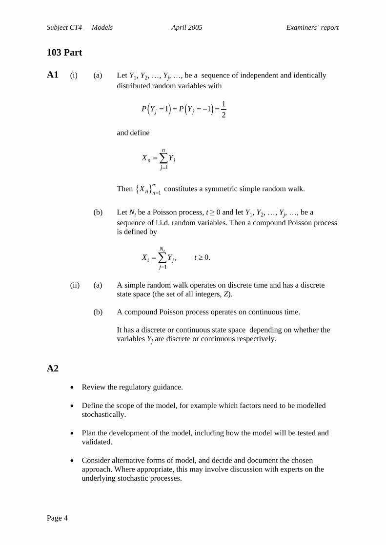
103 Part
A1 (i) (a) Let Y1, Y2, , Yj, , be a sequence of independent and identically distributed random variables with
11 1
2j jP Y P Y
and define
1
n
n jj
X Y
Then 1n n
X constitutes a symmetric simple random walk.
(b) Let Nt be a Poisson process, t 0 and let Y1, Y2, , Yj, , be a sequence of i.i.d. random variables. Then a compound Poisson process is defined by
1
, 0.tN
t jj
X Y t
(ii) (a) A simple random walk operates on discrete time and has a discrete state space (the set of all integers, Z).
(b) A compound Poisson process operates on continuous time.
It has a discrete or continuous state space depending on whether the variables Yj are discrete or continuous respectively.
A2
Review the regulatory guidance.
Define the scope of the model, for example which factors need to be modelled stochastically.
Plan the development of the model, including how the model will be tested and validated.
Consider alternative forms of model, and decide and document the chosen approach. Where appropriate, this may involve discussion with experts on the underlying stochastic processes.

Subject CT4 Models April 2005 Examiners report
Page 5
Collect any data required, for example historic losses or policy data.
Choose parameters. For economic factors should be able to calibrate to market data. For other factors e.g. expenses, claim distributions need to discuss with staff.
Existing worst case scenarios. Discuss with staff who made the estimates, especially to gauge views on the probability of events occurring.
Decide on the software to be used for the model.
Write the computer programs.
Debug the program, for example by checking the model behaves as expected for simple, defined scenarios.
Review the reasonableness of the output. May include:
median outcomes (how do these compare with business plans)
what probability is assigned to worst case scenarios
Test the sensitivity of the model to small changes in parameters.
Calculate the capital requirement.
Communicate findings to management. Document.
Other suitable points were given credit, including:
Validate data.
Run model on historic data to compare model s predictions with previous observations.
Review parameters that have greatest effect on outputs.
Present range of capital requirements for differing parameter inputs.
A3 (i) It is clear that 2kY can only take two values, ±1, with probabilities
2 2 1 2 1 2 1 2 11
1 1 12k k k k kP Y P Y Y P Y Y
and
2
2 1 2 1 2 1 2 1
1
11, 1 1, 1
2
k
k k k k
P Y
P Y Y P Y Y
so that they have the same distribution as Y2k+1.
To show that 2 2 1,k kY Y are independent, we observe first that
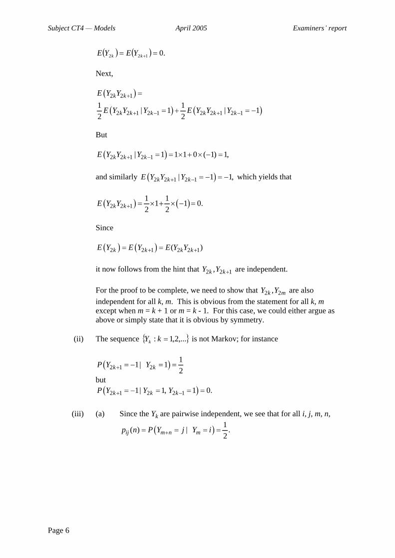
Subject CT4 Models April 2005 Examiners report
Page 6
.0122 kk YEYE
Next,
2 2 1k kE Y Y
2 2 1 2 1 2 2 1 2 11 1
| 1 | 12 2k k k k k kE Y Y Y E Y Y Y
But
2 2 1 2 1| 1 1 1 0 ( 1) 1,k k kE Y Y Y
and similarly 2 2 1 2 1| 1 1,k k kE Y Y Y which yields that
2 2 11 1
1 1 0.2 2k kE Y Y
Since
2 2 1 2 2 1( )k k k kE Y E Y E Y Y
it now follows from the hint that 2 2 1,k kY Y are independent.
For the proof to be complete, we need to show that 2 2,k mY Y are also
independent for all k, m. This is obvious from the statement for all k, m except when m = k + 1 or m = k - 1. For this case, we could either argue as above or simply state that it is obvious by symmetry.
(ii) The sequence ,...2,1: kYk is not Markov; for instance
2 1 21
1| 12k kP Y Y
but
2 1 2 2 11| 1, 1 0.k k kP Y Y Y
(iii) (a) Since the Yk are pairwise independent, we see that for all i, j, m, n, 1
( ) | .2ij m n mp n P Y j Y i
Subject CT4 Models April 2005 Examiners report
Page 7
(b) The probabilities do not depend on the current state as they are all ½
Using the result in (a) we therefore see that
1,1
1 1 1 1 1( ) ( )
2 2 2 2 2ik kjk
p n p r
( ).ijp n r
which shows that the Chapman Kolmogorov equations are satisfied
although ,...2,1: kYk is not Markov.
A4 (i)
NM
M W
D
DIV
0.1
0.025
0.0250.025
0.1
0.025
0.1
0.050.025
(ii) The transitions out of the divorced state are to the same states, and with the same transition probabilities, as the transitions out of state NM. Therefore the probability of ever reaching state W is the same from both states.
Alternatively, this could be shown by producing the equation conditioning on the first move out of DIV, as in part (iii), and showing this is identical to that for NMP .
(iii) Conditioning on the first move out of each state:
0.025 0.1
0.125 0.125
0.025 0.05 0.025
0.1 0.1 0.1
NM D M
M D DIV W
P P P
P P P P
As 1DP and 0WP , these give
Subject CT4 Models April 2005 Examiners report
Page 8
0.025 0.1 1 4
0.125 0.125 5 5
0.025 0.05 1 1
0.1 0.1 4 2
NM M M
M DIV DIV
P P P
P P P
as required.
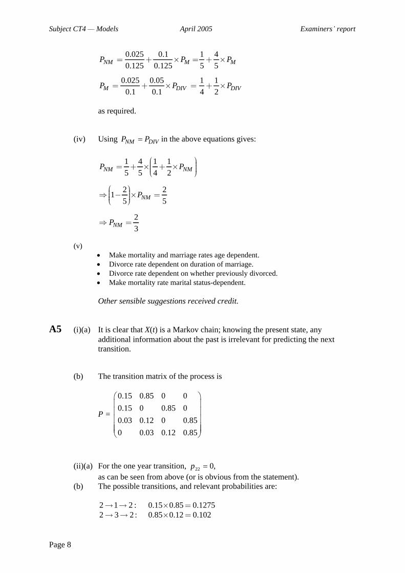
(iv) Using NM DIVP P in the above equations gives:
1 4 1 1
5 5 4 2
2 21
5 5
2
3
NM NM
NM
NM
P P
P
P
(v)
Make mortality and marriage rates age dependent.
Divorce rate dependent on duration of marriage.
Divorce rate dependent on whether previously divorced.
Make mortality rate marital status-dependent.
Other sensible suggestions received credit.
A5 (i)(a) It is clear that X(t) is a Markov chain; knowing the present state, any additional information about the past is irrelevant for predicting the next transition.
(b) The transition matrix of the process is
P =
0.15 0.85 0 0
0.15 0 0.85 0
0.03 0.12 0 0.85
0 0.03 0.12 0.85
(ii)(a) For the one year transition, ,022p as can be seen from above (or is obvious from the statement).
(b) The possible transitions, and relevant probabilities are:
2 1 2 : 0.15 0.85 0.1275
2 3 2 : 0.85 0.12 0.102
Subject CT4 Models April 2005 Examiners report
Page 9
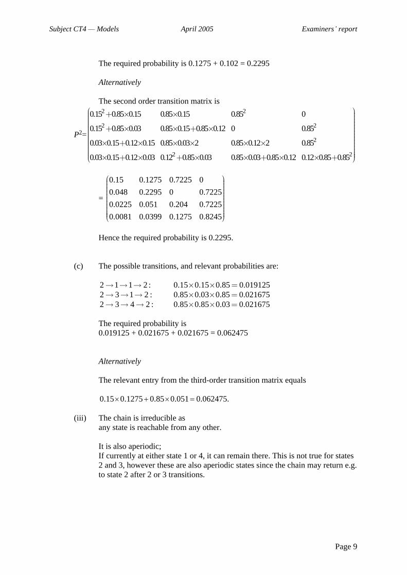
The required probability is 0.1275 + 0.102 = 0.2295
Alternatively
The second order transition matrix is
P2=
2 2
2 2
2
2 2
0.15 0.85 0.15 0.85 0.15 0.85 0
0.15 0.85 0.03 0.85 0.15 0.85 0.12 0 0.85
0.03 0.15 0.12 0.15 0.85 0.03 2 0.85 0.12 2 0.85
0.03 0.15 0.12 0.03 0.12 0.85 0.03 0.85 0.03 0.85 0.12 0.12 0.85 0.85
=
0.15 0.1275 0.7225 0
0.048 0.2295 0 0.7225
0.0225 0.051 0.204 0.7225
0.0081 0.0399 0.1275 0.8245
Hence the required probability is 0.2295.
(c) The possible transitions, and relevant probabilities are:
2 1 1 2 : 0.15 0.15 0.85 0.019125
2 3 1 2 : 0.85 0.03 0.85 0.021675
2 3 4 2 : 0.85 0.85 0.03 0.021675
The required probability is 0.019125 + 0.021675 + 0.021675 = 0.062475
Alternatively
The relevant entry from the third-order transition matrix equals
0.15 0.1275 0.85 0.051 0.062475.
(iii) The chain is irreducible as any state is reachable from any other.
It is also aperiodic; If currently at either state 1 or 4, it can remain there. This is not true for states 2 and 3, however these are also aperiodic states since the chain may return e.g. to state 2 after 2 or 3 transitions.
Subject CT4 Models April 2005 Examiners report
Page 10
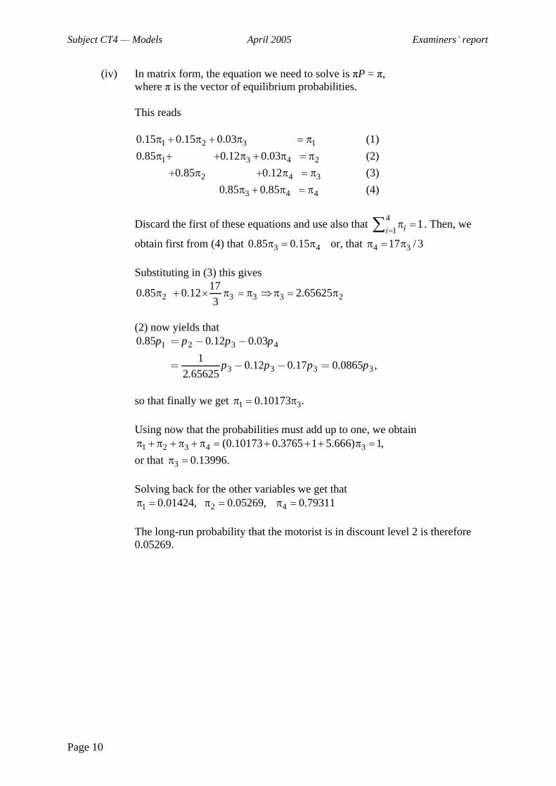
(iv) In matrix form, the equation we need to solve is P = , where is the vector of equilibrium probabilities.
This reads
1 2 3 10.15 0.15 0.03 (1)
1 3 4 20.85 0.12 0.03 (2)
2 4 30.85 0.12 (3)
3 4 40.85 0.85 (4)
Discard the first of these equations and use also that 4
11ii
. Then, we
obtain first from (4) that 3 40.85 0.15 or, that 4 317 / 3
Substituting in (3) this gives
2 3 3 3 217
0.85 0.12 2.656253
(2) now yields that
1 2 3 4
3 3 3 3
0.85 0.12 0.03
10.12 0.17 0.0865 ,
2.65625
p p p p
p p p p
so that finally we get 1 30.10173 .
Using now that the probabilities must add up to one, we obtain
1 2 3 4 3(0.10173 0.3765 1 5.666) 1,
or that 3 0.13996.
Solving back for the other variables we get that
1 2 40.01424, 0.05269, 0.79311
The long-run probability that the motorist is in discount level 2 is therefore 0.05269.
Subject CT4 Models April 2005 Examiners report
Page 11
A6 (i)
No Breakdowns
One Breakdown
Two Breakdowns
Three Breakdowns
1/10 1/5 1/4
(ii) 0 01
( ) ( )10
P t P t
1 0 11 1
( ) ( ) ( )10 5
P t P t P t
2 1 21 1
( ) ( ) ( )5 4
P t P t P t
(iii)(a) Dividing the first equation by 0 ( )P t :
01
ln ( )10
dP t
dt
Hence, using the boundary condition 0 (0) 1P
100( )
t
P t e
(b) Substitute into the second equation above to obtain
101 1
1 1( ) * ( )
10 5
t
P t e P t
Using an integrating factor 5et
, we get
'5 10 51 1
1 1e ( ) e
5 10
t t t
P t P t
5 101
1( )
10
t td
e P t edt
5 101( )
t t
e P t e const
10 51( )
t t
P t e const e
Subject CT4 Models April 2005 Examiners report
Page 12
10 51( ) exp exp
t t
P t
using boundary condition 1(0) 0P
Alternatively
Differentiate the suggested solution and verify it obeys the second equation.
And that the boundary condition is satisfied.
(iv) Proceeding in a similar way with the equation for 2 ( )P t
10 52 2
1 1 1( ) exp exp * ( )
5 5 4
t t
P t P t
3 120 204
21
exp ( ) (exp exp )5
tt td
P tdt
3 120 204
24 8
exp ( ) exp 4 exp3 3
tt t
P t
10 5 42
4( ) [exp 3 exp 2 exp ]
3
t t t
P t
(v) 1 23
Expected Claims 1 (1) 2 (1) 3 (1)ii
P P P
1 2 0 1 2(1) 2 (1) 3 1 (1) (1) (1)P P P P P
1/100(1) exp 0.905P
1/10 1/51(1) exp exp 0.0861P
1 1 110 5 4
24
(1) [exp 3 exp 2 exp ] 0.008328963
P
Substituting these values gives:
Expected Claims = 0.1049
Subject CT4 Models April 2005 Examiners report
Page 13
104 Part
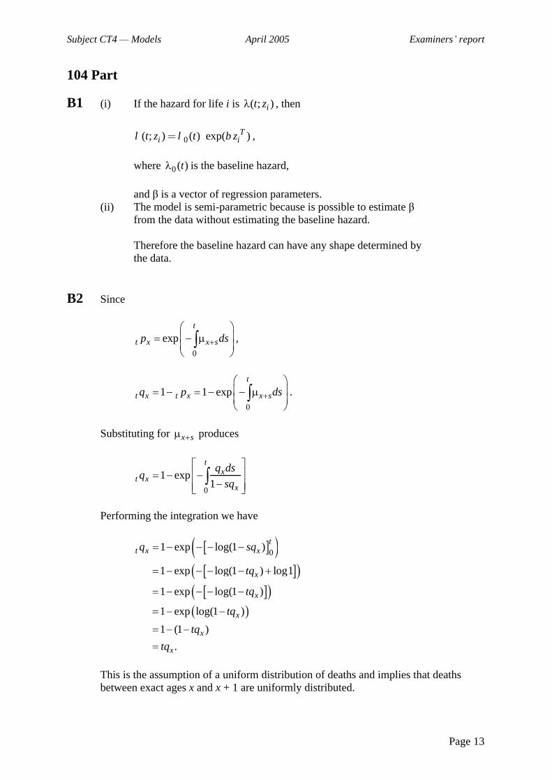
B1 (i) If the hazard for life i is ( ; )it z , then
0( ; ) ( ) exp( )Ti it z t zl l b ,
where 0( )t is the baseline hazard,
and is a vector of regression parameters. (ii) The model is semi-parametric because is possible to estimate
from the data without estimating the baseline hazard.
Therefore the baseline hazard can have any shape determined by the data.
B2 Since
0
expt
t x x sp ds ,
0
1 1 expt
t x t x x sq p ds .
Substituting for x s produces
0
1 exp1
tx
t xx
q dsq
sq
Performing the integration we have
01 exp log(1 )
1 exp log(1 ) log1
1 exp log(1 )
1 exp log(1 )
1 (1 )
.
tt x x
x
x
x
x
x
q sq
tq
tq
tq
tq
tq
This is the assumption of a uniform distribution of deaths and implies that deaths between exact ages x and x + 1 are uniformly distributed.
Subject CT4 Models April 2005 Examiners report
Page 14
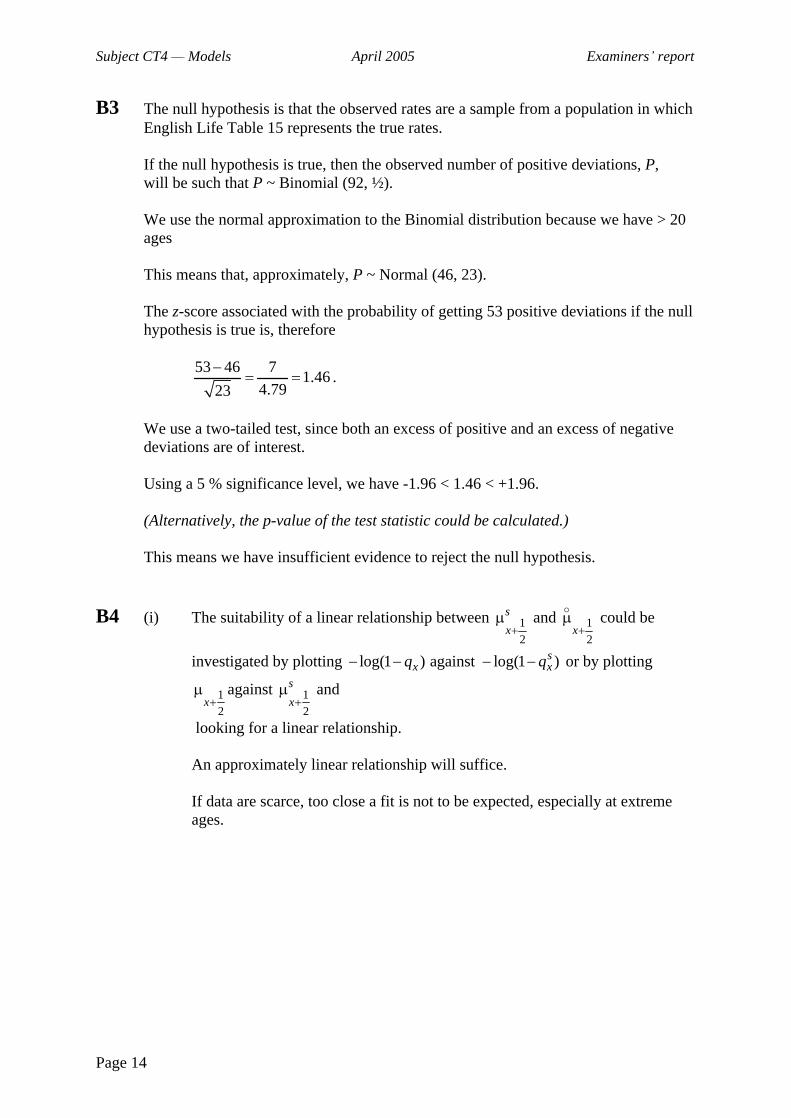
B3 The null hypothesis is that the observed rates are a sample from a population in which English Life Table 15 represents the true rates.
If the null hypothesis is true, then the observed number of positive deviations, P, will be such that P ~ Binomial (92, ½).
We use the normal approximation to the Binomial distribution because we have > 20 ages
This means that, approximately, P ~ Normal (46, 23).
The z-score associated with the probability of getting 53 positive deviations if the null hypothesis is true is, therefore
53 46 71.46
4.7923.
We use a two-tailed test, since both an excess of positive and an excess of negative deviations are of interest.
Using a 5 % significance level, we have -1.96 < 1.46 < +1.96.
(Alternatively, the p-value of the test statistic could be calculated.)
This means we have insufficient evidence to reject the null hypothesis.
B4 (i) The suitability of a linear relationship between 12
s
x and 1
2x
could be
investigated by plotting log(1 ) against log(1 )sx xq q or by plotting
12
xagainst 1
2
s
x and
looking for a linear relationship.
An approximately linear relationship will suffice.
If data are scarce, too close a fit is not to be expected, especially at extreme ages.
Subject CT4 Models April 2005 Examiners report
Page 15
(ii) (a) We can work with either sxq or 1
2
s
x.
The value of k which minimises either
2( )x x xx
w q q
or 2
1 12 2
xx x
x
w
should be found (note that the summations are over all relevant ages x)
At each age there will be a different sample size or exposed to risk, Ex. This will usually be largest at ages where many term assurances are sold (e.g. ages 25 to 50 years) and smaller at other ages.
(b) The estimation procedure should pay more attention to ages where there are lots of data. These ages should have a greater influence on the choice of k than other ages.
This implies weights wx
Ex. A suitable choice would be
12
1 1 or
var varx xx
x
w wq
or wx = Ex
(iii) The graduated forces of mortality are a linear function of the forces in the standard table.
Since the forces in the standard table should already be smooth, a linear function of them will also be smooth.
B5 (i) Consider the durations tj at which events take place. Let the number of deaths at duration tj be dj and the number of insects still at risk of death at duration tj be nj.
At tj = 1, S(t) falls from 1.0000 to 0.9167.
Since the Kaplan-Meier estimate of S(t) is
( ) (1 ( ))j
jt t
S t t ,
Subject CT4 Models April 2005 Examiners report
Page 16
we must have 0.9167 1 (1) ,
so that (1) 0.0833.
Since 1
1(1)
d
n, then we have 1
10.0833
d
n,
and, since all 12 insects are at risk of dying at tj = 1, we must therefore have d1 = 1 and n1 = 12.
Similarly, at tj = 3, we must have 0.7130 0.9167(1 (3))
so that 3
3
0.9167 0.7130(3) 0.222
0.9167
d
n.
Since we can have at most 11 insects in the risk set at tj = 3, we must have d3 = 2 and n3 = 9. Similarly, at tj = 6, we must have 0.4278 0.7130(1 (6)) ,
so that 6
6
0.7130 0.4278(6) 0.400
0.7130
d
n.
Since we can have at most 7 insects in the risk set at tj = 6, we must have d6 = 2 and n6 = 5.
Therefore 2 insects died at duration 3 weeks and 2 insects died at duration 6 weeks.
Alternatively
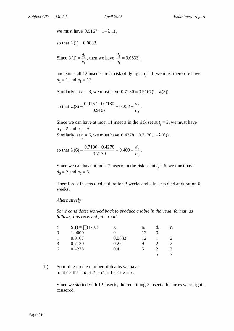
Some candidates worked back to produce a table in the usual format, as follows; this received full credit.
t S(t) = (1- t) t nt dt ct
0 1.0000 0 12 0 1 0.9167 0.0833 12 1 2 3 0.7130 0.22 9 2 2 6 0.4278 0.4 5 2
3
5 7
(ii) Summing up the number of deaths we have total deaths = 1 3 6 1 2 2 5d d d .
Since we started with 12 insects, the remaining 7 insects histories were right-censored.
Subject CT4 Models April 2005 Examiners report
Page 17
B6 (i) The principle of correspondence states that a life alive at time t should be included in the exposure at age x at time t if and only if were that life to die immediately, he or she would be counted in the deaths data x at age x.
(ii) Px(t) is the number of policies under observation aged x nearest birthday on 1 January in year t.
To correspond with the claims data, we wish to have policies classified by age last birthday.
Let the number of policies aged x last birthday on 1 January in year t be ( )xP t .
Then, assuming that birthdays are evenly distributed,
11
( ) ( ) ( )2x x xP t P t P t .
The central exposed to risk is then given by 1
0
( )cx xE P t dt .
Using the trapezium approximation this is
1( ) ( 1)
2cx x xE P t P t ,
and, substituting for the ( )xP t in terms of Px(t) from the equation above
produces
1 11 1 1
( ) ( ) ( 1) ( 1)2 2 2
cx x x x xE P t P t P t P t .
(iii) The principle of correspondence still holds, because we are dealing with claims and policies: one policy can only lead to one claim.
However, because one life may have more than one policy it is possible that two distinct death claims are the result of the death of the same life.
Therefore claims are not independent, whereas deaths are.
Subject CT4 Models April 2005 Examiners report
Page 18
The effect of this is to increase the variance of the number of claims (compared to the situation in which each life has one and only one policy) by the ratio
2i
i
ii
i
i,
where i is the proportion of the lives in the investigation owning i policies (i = 1, 2, 3, ...).
Typically the ratio will vary for each age x.
B7 (i)(a) The two-state estimate of 70 is 70
70
d
v, where v70 is the total time the members
of the sample are under observation between exact ages 70 and 71 years.
70 70,ii
v v ,
where 70,iv is the duration that sample member i is under observation between
exact ages 70 and 71 years.
For each sample member, 70,iv = ENDDATE STARTDATE
where ENDDATE is the earliest of the date at which the observation of that member ceases and the date of the member s 71st birthday, and STARTDATE is the latest of the date at which observation of that member begins and the date of the member s 70th birthday.
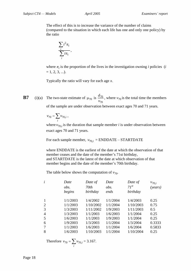
The table below shows the computation of v70.
i Date Date of Date Date of v70,i
obs. 70th obs. 71st (years) begins birthday ends birthday
1 1/1/2003 1/4/2002 1/1/2004 1/4/2003 0.25 2 1/1/2003 1/10/2002 1/1/2004 1/10/2003 0.75 3 1/3/2003 1/11/2002 1/9/2003 1/11/2003 0.5 4 1/3/2003 1/1/2003 1/6/2003 1/1/2004 0.25 5 1/6/2003 1/1/2003 1/9/2003 1/1/2004 0.25 6 1/9/2003 1/3/2003 1/1/2004 1/3/2004 0.3333 7 1/1/2003 1/6/2003 1/1/2004 1/6/2004 0.5833 8 1/6/2003 1/10/2003 1/1/2004 1/10/2004 0.25
Therefore 70 70,ii
v v = 3.167.
Subject CT4 Models April 2005 Examiners report
Page 19
We observed two deaths (members 3 and 4), so
702
0.63163.167
.
(b) 70 701 exp( )q
1 exp( 0.6316) 1 0.5318 0.4682.
(ii) The contributions to the Poisson likelihood made by each member are proportional to the following
Member 1 exp(-0.25 70 )
2 exp(-0.75 70 )
3 70 exp(-0.5 70 )
4 70 exp(-0.25 70 )
5 exp(-0.25 70 )
6 exp(-0.3333 70 )
7 exp(-0.5833 70 )
8 exp(-0.25 70 )
The total likelihood, L, is proportional to the product
270 70[exp( 3.167 )]( ) .L
Then
70 70log 3.167 2logL
so that
70 70
log 23.167 .
d L
d
Setting this equal to zero and solving for 70 produces the maximum
likelihood estimate, which is 2/3.167 = 0.6316
Since 2
2 270 70
log 2d L
d, which is always negative, we definitely have a
maximum.
This is the same as the estimate from the two-state model.

Subject CT4 Models April 2005 Examiners report
Page 20
(iii) The Poisson model is not an exact model, since it allows for a non-zero probability of more than n deaths in a sample of size n.
The variance of the maximum likelihood estimator for the two-state model is only available asymptotically, whereas that for the Poisson model is available exactly in terms of the true .
The two-state model extends to processes with increments, whereas the Poisson model does not.
The Poisson model is a less satisfactory approximation to the multiple state model when transition rates are high.

Faculty of Actuaries Institute of Actuaries
EXAMINATION
14 September 2005 (am)
Subject CT4 (103)
Models (103 Part) Core Technical
Time allowed: One and a half hours
INSTRUCTIONS TO THE CANDIDATE
1. Enter all the candidate and examination details as requested on the front of your answer booklet.
2. You must not start writing your answers in the booklet until instructed to do so by the supervisor.
3. Mark allocations are shown in brackets.
4. Attempt all 7 questions, beginning your answer to each question on a separate sheet.
5. Candidates should show calculations where this is appropriate.
Graph paper is not required for this paper.
AT THE END OF THE EXAMINATION
Hand in BOTH your answer booklet, with any additional sheets firmly attached, and this question paper.
In addition to this paper you should have available the 2002 edition of the Formulae and Tables and your own electronic calculator.
Faculty of Actuaries CT4 (103) S2005 Institute of Actuaries
CT4 (103) S2005 2
1 An insurance company has a block of in-force business under which policyholders have been given options and investment-related guarantees. A stochastic model has been developed which projects option and guarantee costs. You have used the model to estimate, for the Company Board, the probability of the insurance company having insufficient assets to honour the payouts under the policies. A Board member has asked whether there are any factors which could cause this probability to be inaccurate.
Outline the items you would mention in your response. [5]
2 (i) In the context of a stochastic process denoted by {Xt : t
J}, define:
(a) state space (b) time set (c) sample path
[2]
(ii) Stochastic process models can be placed in one of four categories according to whether the state space is continuous or discrete, and whether the time set is continuous or discrete. For each of the four categories:
(a) State a stochastic process model of that type.
(b) Give an example of a problem an actuary may wish to study using a model from that category.
[4] [Total 6]
3 A die is rolled repeatedly. Consider the following two sequences:
I Bn is the largest number rolled in the first n outcomes. II Cn is the number of sixes rolled in the first n outcomes.
For each of these two sequences:
(a) Explain why it is a Markov chain. (b) Determine the state space of the chain. (c) Derive the transition probabilities. (d) Explain whether the chain is irreducible and/or aperiodic. (e) Describe the equilibrium distribution of the chain. [7]
CT4 (103) S2005 3 PLEASE TURN OVER
4 A life insurance company prices its long-term sickness policies using a three-state Markov model in continuous time. The states are healthy (H), ill (I) and dead (D). The forces of transition in the model are HI = , IH = , HD = , ID = v and they are assumed to be constant over time.
For a group of policyholders observed over a 1-year period, there are:
23 transitions from State to State ; 15 transitions from State to State ; 3 deaths from State ; 5 deaths from State .
The total time spent in State H is 652 years and the total time spent in State I is 44 years.
(i) Write down the likelihood function for these data. [3]
(ii) Derive the maximum likelihood estimate of . [2]
(iii) Estimate the standard deviation of , the maximum likelihood estimator of . [2]
[Total 7]
5 Claims arrive at an insurance company according to a Poisson process with rate
per week.
Assume time is expressed in weeks.
(i) Show that, given that there is exactly one claim in the time interval [t, t + s], the time of the claim arrival is uniformly distributed on [t, t + s]. [3]
(ii) State the joint density of the holding times T0, T1, , Tn between successive claims. [1]
(iii) Show that, given that there are n claims in the time interval [0, t], the number of claims in the interval [0, s] for s < t is binomial with parameters n and s/t.
[3] [Total 7]
CT4 (103) S2005 4
6 A Markov jump process Xt with state space S = {0, 1, 2, , N} has the following transition rates:
ii =
for 0
i
N 1
i,i+1 =
for 0
i
N 1
ij = 0 otherwise
(i) Write down the generator matrix and the Kolmogorov forward equations (in component form) associated with this process. [3]
(ii) Verify that for 0
i
N 1 and for all j i, the function
( )( ) =
( )!
j it
ijt
p t ej i
is a solution to the forward equations in (i). [2]
(iii) Identify the distribution of the holding times associated with the jump process. [2]
[Total 7]
7 A time-inhomogeneous Markov jump process has state space {A, B} and the transition rate for switching between states equals 2t, regardless of the state currently occupied, where t is time.
The process starts in state A at t = 0.
(i) Calculate the probability that the process remains in state A until at least time s. [2]
(ii) Show that the probability that the process is in state B at time T, and that it is
in the first visit to state B, is given by 22 exp TT . [3]
(iii) (a) Sketch the probability function given in (ii).
(b) Give an explanation of the shape of the probability function.
(c) Calculate the time at which it is most likely that the process is in its first visit to state B.
[6] [Total 11]
END OF PAPER

Faculty of Actuaries Institute of Actuaries
EXAMINATION
14 September 2005 (am)
Subject CT4 (104)
Models (104 Part) Core Technical
Time allowed: One and a half hours
INSTRUCTIONS TO THE CANDIDATE
1. Enter all the candidate and examination details as requested on the front of your answer booklet.
2. You must not start writing your answers in the booklet until instructed to do so by the supervisor.
3. Mark allocations are shown in brackets.
4. Attempt all 6 questions, beginning your answer to each question on a separate sheet.
5. Candidates should show calculations where this is appropriate.
Graph paper is not required for this paper.
AT THE END OF THE EXAMINATION
Hand in BOTH your answer booklet, with any additional sheets firmly attached, and this question paper.
In addition to this paper you should have available the 2002 edition of the Formulae and Tables and your own electronic calculator.
Faculty of Actuaries CT4 (104) S2005 Institute of Actuaries

CT4 (104) S2005 2
1 Describe the advantages and disadvantages of graduating a set of observed mortality rates using a parametric formula. [4]
2 A lecturer at a university gives a course on Survival Models consisting of 8 lectures. 50 students initially register for the course and all attend the first lecture, but as the course proceeds the numbers attending lectures gradually fall.
Some students switch to another course. Others intend to sit the Survival Models examination but simply stop attending lectures because they are so boring. In this university, students who decide not to attend a lecture are not permitted to attend any subsequent lectures.
The table below gives the number of students switching courses and stopping attending lectures after each of the first 7 lectures of the course.
Lecture number
Number of students switching courses
Number of students ceasing to attend lectures but remaining registered for Survival Models
1 5 1 2 3 0 3 2 3 4 0 1 5 0 2 6 0 1 7 0 0
The university s Teaching Quality Monitoring Service has devised an Index of Lecture Boringness. This index is defined as the Kaplan-Meier estimate of the proportion of students remaining registered for the course who attend the final lecture. In calculating the Index, students who switch courses are to be treated as censored after the last lecture they attend.
(i) Calculate the Index of Lecture Boringness for the Survival Models course. [4]
(ii) Explain whether the censoring in this example is likely to be non-informative. [2]
[Total 6]
CT4 (104) S2005 3 PLEASE TURN OVER
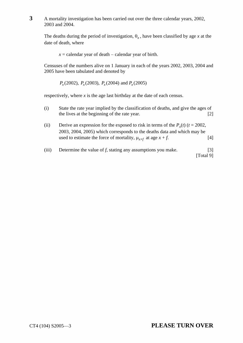
3 A mortality investigation has been carried out over the three calendar years, 2002, 2003 and 2004.
The deaths during the period of investigation, x , have been classified by age x at the date of death, where
x = calendar year of death calendar year of birth.
Censuses of the numbers alive on 1 January in each of the years 2002, 2003, 2004 and 2005 have been tabulated and denoted by
(2002), (2003), (2004) and (2005)x x x xP P P P
respectively, where x is the age last birthday at the date of each census.
(i) State the rate year implied by the classification of deaths, and give the ages of the lives at the beginning of the rate year. [2]
(ii) Derive an expression for the exposed to risk in terms of the Px(t) (t = 2002, 2003, 2004, 2005) which corresponds to the deaths data and which may be used to estimate the force of mortality, x+f at age x + f. [4]
(iii) Determine the value of f, stating any assumptions you make. [3] [Total 9]
CT4 (104) S2005 4
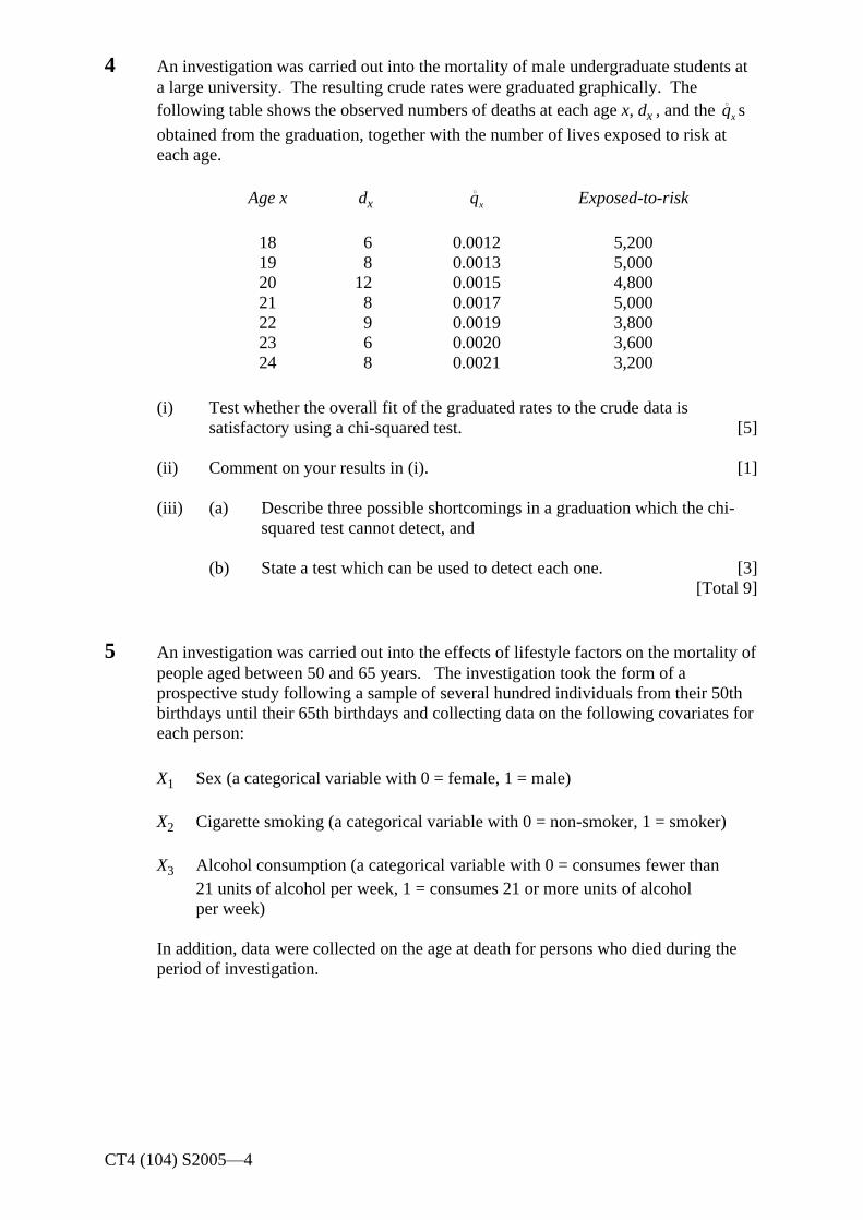
4 An investigation was carried out into the mortality of male undergraduate students at a large university. The resulting crude rates were graduated graphically. The following table shows the observed numbers of deaths at each age x, dx , and the xq s
obtained from the graduation, together with the number of lives exposed to risk at each age.
Age x dx xq
Exposed-to-risk
18 6 0.0012 5,200 19 8 0.0013 5,000 20 12 0.0015 4,800 21 8 0.0017 5,000 22 9 0.0019 3,800 23 6 0.0020 3,600 24 8 0.0021 3,200
(i) Test whether the overall fit of the graduated rates to the crude data is satisfactory using a chi-squared test. [5]
(ii) Comment on your results in (i). [1]
(iii) (a) Describe three possible shortcomings in a graduation which the chi-squared test cannot detect, and
(b) State a test which can be used to detect each one. [3] [Total 9]
5 An investigation was carried out into the effects of lifestyle factors on the mortality of people aged between 50 and 65 years. The investigation took the form of a prospective study following a sample of several hundred individuals from their 50th birthdays until their 65th birthdays and collecting data on the following covariates for each person:
X1 Sex (a categorical variable with 0 = female, 1 = male)
X2 Cigarette smoking (a categorical variable with 0 = non-smoker, 1 = smoker)
X3 Alcohol consumption (a categorical variable with 0 = consumes fewer than 21 units of alcohol per week, 1 = consumes 21 or more units of alcohol per week)
In addition, data were collected on the age at death for persons who died during the period of investigation.
CT4 (104) S2005 5 PLEASE TURN OVER
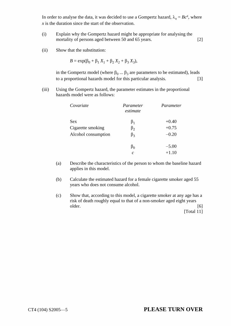
In order to analyse the data, it was decided to use a Gompertz hazard, x = Bcx, where x is the duration since the start of the observation.
(i) Explain why the Gompertz hazard might be appropriate for analysing the mortality of persons aged between 50 and 65 years. [2]
(ii) Show that the substitution:
B = exp( 0 + 1 X1 + 2 X2 + 3 X3),
in the Gompertz model (where 0 ... 3 are parameters to be estimated), leads to a proportional hazards model for this particular analysis. [3]
(iii) Using the Gompertz hazard, the parameter estimates in the proportional hazards model were as follows:
Covariate Parameter Parameter estimate
Sex 1 +0.40 Cigarette smoking 2 +0.75
Alcohol consumption 3 0.20
0 5.00 c +1.10
(a) Describe the characteristics of the person to whom the baseline hazard applies in this model.
(b) Calculate the estimated hazard for a female cigarette smoker aged 55 years who does not consume alcohol.
(c) Show that, according to this model, a cigarette smoker at any age has a risk of death roughly equal to that of a non-smoker aged eight years older. [6]
[Total 11]

CT4 (104) S2005 6
6 Studies of the lifetimes of a certain type of electric light bulb have shown that the probability of failure, q0 , during the first day of use is 0.05 and after the first day of
use the force of failure , x , is constant at 0.01.
(i) Calculate the probability that a light bulb will fail within the first 20 days. [2]
(ii) Calculate the complete expectation of life (in days) of:
(a) a one-day old light bulb (b) a new light bulb
[7]
(iii) Comment on the difference between the complete expectations of life calculated in (ii) (a) and (b). [2]
[Total 11]
END OF PAPER

Faculty of Actuaries Institute of Actuaries
EXAMINATION
September 2005
Subject CT4
Models (includes both 103 and 104 parts) Core Technical
EXAMINERS REPORT
Faculty of Actuaries Institute of Actuaries

Subject CT4 Models September 2005 Examiners Report
Page 2
EXAMINERS COMMENTS
Comments on solutions presented to individual questions for this September 2005 paper are given below:
103 Part
Question A1 This was not well answered. There was a lot of repetition in some of the solutions offered - for example several different instances of parameter error may have been mentioned.
Question A2 This was well answered overall, even by the weaker candidates. Credit was not given in part (ii)(b) if the examples cited were not likely to be encountered by an actuary working in a professional capacity.
Question A3 This was well answered overall. Some candidates lost marks by not explaining why the chains were not irreducible and were aperiodic. Many candidates did not correctly identify the state space of the chain Cn and most did not realise that the chain will escape to infinity as the value increases without barrier.
Question A4 This was very well answered overall, with the majority of candidates scoring highly. One common mistake was the omission of the constant term from the likelihood function in part (i).
Question A5 This was very poorly answered by all but a few candidates. Some candidates offered general explanations in parts (i) and (iii), which, if clear enough, were given some credit.
Question A6 Overall this was not well answered. In part (i), few candidates gave the full, correct Kolmogorov equations. Many candidates lost marks in part (ii) because of insufficient or inaccurate working.
Question A7 Overall this was not well answered. However, part (i) was well answered. Some candidates reached the correct answer via a different solution and received full credit. Many candidates struggled with part (ii), failing to identify the correct integrand required. In part (iii), many candidates described the shape of the function, but few explained it, as required by the question.
Subject CT4 Models September 2005 Examiners Report
Page 3
104 Part
Question B1 This was not well answered. Some candidates commented on the advantages/disadvantages of graduation in general, rather than concentrating on the parametric formula method.
Question B2 Part (i) was well answered. In part (ii), many candidates clearly did not understand the meaning of non-informative censoring.
Question B3 This was well answered overall. In part (ii), the question asked candidates to derive an expression and therefore we were looking for clearly set out steps here. Many candidates lost marks by not providing sufficient explanation of their working.
Question B4 This was very well answered, even by the weaker candidates. The main areas where candidates lost marks were: not stating the null hypothesis, or not stating it clearly enough; failure to identify the correct degrees of freedom to be used in the test; and insufficient or insufficiently clear descriptions of the shortcomings. In part (iii), the majority of candidates seemed confused between two issues in connection with bias. There are two distinct problems. Firstly, if the consistent bias is only small, the chi-squared test may fail to detect it because the resulting number (i.e. the sum of the squared deviations) is not large enough to exceed the critical value. The signs test, which ignores the magnitude of the bias and looks only at how consistent it is across the ages, can be used to identify this. The second problem is that even if the consistent bias is larger and the chi-squared test leads us to reject the null hypothesis, the test gives no indication of whether the graduated rates are too high or too low. This is because the deviations are squared and the test statistic always positive. The signs test is not a solution to this second problem.
Question B5 This was well answered overall. Some parts of the question required candidates to show a result; candidates lost marks if their working was not sufficiently clear or complete.
Question B6 This was not well answered. Surprisingly few candidates correctly answered part (i). In parts (ii) and (iii), very few candidates recognised that the expectation of life was an average of the future lifetimes of those bulbs still shining. As a result, although many candidates correctly calculated the expectation of life for a one-day old bulb, few managed to do so for a new bulb. In part (iii), most candidates commented on the higher force of failure in the first day.

Subject CT4 Models September 2005 Examiners Report
Page 4
103 Part
A1
Items to be mentioned include:
Models will be chosen which it is felt give a reasonable reflection of the underlying real world processes, but this may not turn out to be the case. (Model error.)
The model may be very sensitive to parameters chosen, and the parameters are estimates because the true underlying parameters cannot be observed. (Parameter error.)
Sampling error may result from running insufficient simulations. (It should be possible to give a confidence interval for the error that could result from this source.)
The management actions assumed may not match what would happen in extreme circumstances.
Policyholder behaviour, such as take-up rates for options, may differ in practice.
There may be future events, such as legislative changes which affect the interpretation of the policy conditions, which have not been anticipated in the modelling.
There may be errors in the coding of the model. The model is likely to be complex and difficult to verify completely.
The model relies on input data, which may be grouped rather than being able to run every policy. Any errors in the data could cause the output to be inaccurate.
Subject CT4 Models September 2005 Examiners Report
Page 5
A2
(i) (a) The state space is the set of values which it is possible for each random variable Xt to take.
(b) The time set is the set J, the times at which the process contains a random variable Xt.
(c) A sample path is a joint realisation of the variables Xt for all t in J, that is a set of values for Xt (at each time in the time set) calculated using the previous values for Xt in the sample path.
(ii) Discrete State Space, Discrete Time
(a) Simple random walk, Markov chain, or any other suitable example
(b) Any reasonable example. For example: No Claims Discount systems, Credit Rating at end of each year
Discrete State Space, Continuous Time
(a) Poisson process, Markov jump process, for example
(b) Any reasonable example. For example: Claims received by an insurer, Status of pension scheme member
Continuous State Space, Discrete Time
(a) General random walk, time series, for example
(b) Any reasonable example. For example: Share prices at end of each trading day, Inflation index
Continuous State Space, Continuous Time
(a) Brownian motion, diffusion or Itô process, for example. Compound Poisson process if the defined state space is continuous.
(b) Any reasonable example. For example: Share prices during trading period, Value of claims received by insurer
Subject CT4 Models September 2005 Examiners Report
Page 6
A3 (a) Given the current state (the largest outcome or the number of sixes) up to the nth roll, no additional information is required to predict the status of the chain after the next roll. Therefore both Bn and Cn have the Markov property.
(b) Bn has state space {1, 2, 3, 4, 5, 6}, the state space for Cn is the set of non-negative integers.
(c) For Bn, and 1 i, j 6,
1 |6n ni
P B j B i for j = i,
11
|6n nP B j B i
for each j >i
and 1 | 0n nP B j B i
for i > j
For Cn, and for k = 0,1,2, ,
11
1|6n nP C k C k ,
15
|6n nP C k C k ,
and 1 | 0n nP C j C k for all other , 1j k k
(d) The chain Bn is clearly aperiodic; if currently at state i, it can remain there if the next outcome is at most i. It is not irreducible, as it cannot be reached from j for i < j.
Cn is again aperiodic; if currently at state i, it can remain there if the next outcome is not a 6. It is not irreducible; state k cannot be reached from m if k < m.
(e) In the long run, Bn will reach state 6 and will remain there; hence in equilibrium P(Bn = 6) = 1 for sufficiently large n.
Cn cannot decrease and has an infinite state space; therefore, it is certain that it will escape to infinity with probability one.

Subject CT4 Models September 2005 Examiners Report
Page 7
A4 (i) The likelihood is
23 15 3 5exp( 652( ))exp( 44( ))L K
(ii) l = ln L = 652 +23 ln + constant with respect to
Differentiating with respect to
gives
23652
l
and setting equal to zero gives
230 652
230.0353
652
p.a.
Differentiating again gives
2
2 2
230
l
therefore is the maximum likelihood estimate
(iii) The variance of is
12 2
2 23
l,
which we can estimate by 2
.23
Therefore the estimated standard deviation of is 0.00736.23
Subject CT4 Models September 2005 Examiners Report
Page 8
A5 (i) Let Nt denote the number of claims up to time t. Since the Poisson process has stationary increments, we may take t = 0, so that the required conditional distribution is
00
, 1| 1
1
1, 0
1
ss
s
y s y
s
P T y NP T y N
P N
P N N N
P N
But Ns Ny is independent of Ny
and has the same distribution as Ns y.
Thus the right hand side above equals
( )( ),
y s y
s
ye e y
sse
which is the cdf of the uniform distribution on [0, s].
(ii) Since holding times are independent, each having an exponential distribution, their joint density is
1 2
1 2
..., ,..., 0 .1n
n
t t tnt t te
(iii) We have, as in part (i),
,|
,
s ts t
t
s t s
t
P N k N nP N k N n
P N n
P N k N N n k
P N n
Using again that the Poisson process has stationary and independent increments, and that the number of claims in an interval [0, t] is Poisson ( t), we derive from above that
Subject CT4 Models September 2005 Examiners Report
Page 9
( )( ) ( )
! ( )!|
( )
!
( ) !
!( )!
! ( )
!( )!
1
s k t s n k n k
s t t n
t n k n k
t n n
k n k
k n k
k n k
e s e t s
k n kP N k N n
e t
n
e s t s n
k n k e t
n s t s
k n k t t
n s s
k t t
which is binomial with parameters n and s/t.
Subject CT4 Models September 2005 Examiners Report
Page 10
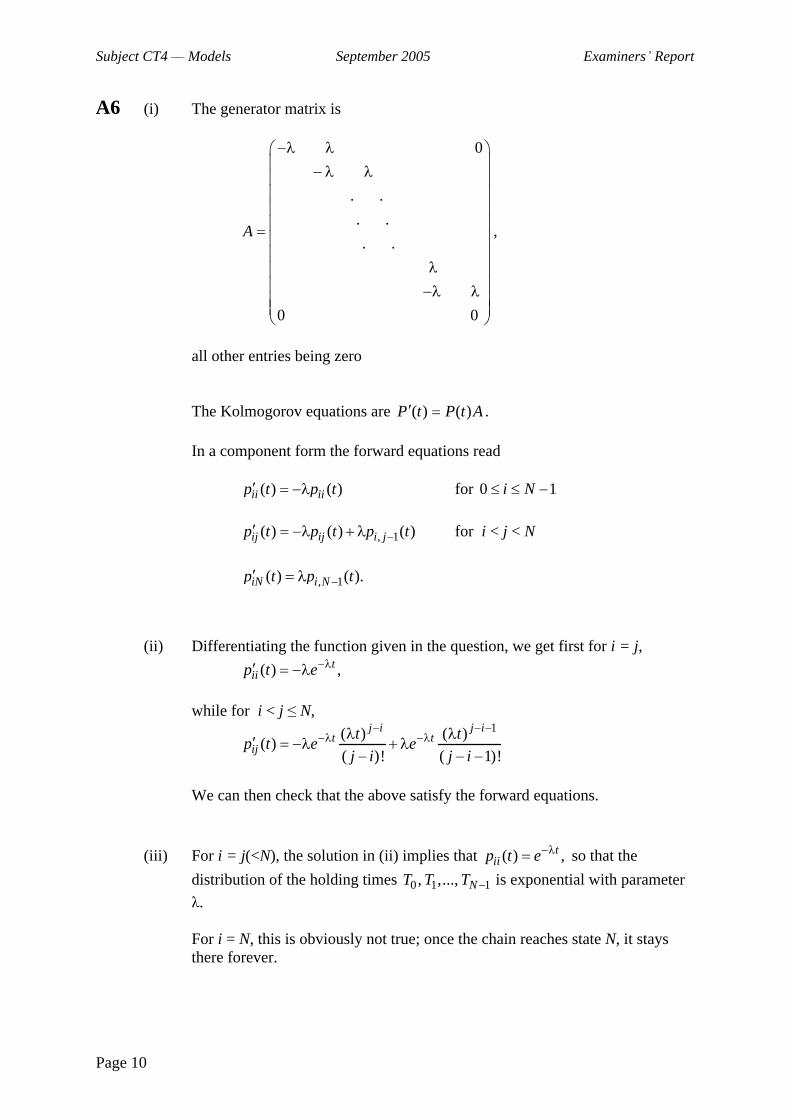
A6 (i) The generator matrix is
0
. .
. .
. .
0 0
A ,
all other entries being zero
The Kolmogorov equations are AtPtP )()( .
In a component form the forward equations read
( ) ( )ii iip t p t
for 0 1i N
, 1( ) ( ) ( )ij ij i jp t p t p t
for i < j < N
, 1( ) ( ).iN i Np t p t
(ii) Differentiating the function given in the question, we get first for i = j,
( ) ,tiip t e
while for i < j N, 1( ) ( )
( )( )! ( 1)!
j i j it t
ijt t
p t e ej i j i
We can then check that the above satisfy the forward equations.
(iii) For i = j(<N), the solution in (ii) implies that ( ) ,tiip t e so that the
distribution of the holding times 0 1 1, ,..., NT T T is exponential with parameter
.
For i = N, this is obviously not true; once the chain reaches state N, it stays there forever.
Subject CT4 Models September 2005 Examiners Report
Page 11
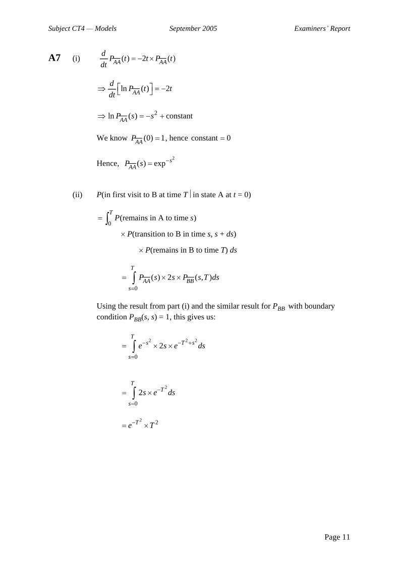
A7 (i) ( ) 2 ( )AA AAd
P t t P tdt
ln ( ) 2
AA
dP t t
dt
2ln ( ) constant
AAP s s
We know (0) 1AA
P , hence constant 0
Hence, 2
( ) exp sAAP s
(ii) P(in first visit to B at time T in state A at t = 0)
0(remains in A to time )
TP s
P(transition to B in time s, s + ds)
P(remains in B to time T) ds
0
( ) 2 ( , )T
AA BBs
P s s P s T ds
Using the result from part (i) and the similar result for PBB with boundary condition PBB(s, s) = 1, this gives us:
2 2 2
0
2T
s T s
s
e s e ds
2
0
2T
T
s
s e ds
2 2Te T
Subject CT4 Models September 2005 Examiners Report
Page 12
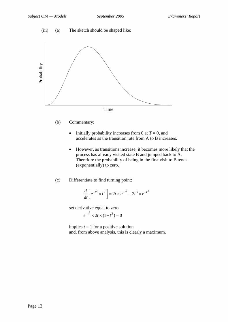
(iii) (a) The sketch should be shaped like:
(b) Commentary:
Initially probability increases from 0 at T = 0, and accelerates as the transition rate from A to B increases.
However, as transitions increase, it becomes more likely that the process has already visited state B and jumped back to A. Therefore the probability of being in the first visit to B tends (exponentially) to zero.
(c) Differentiate to find turning point:
2 2 22 32 2t t tde t t e t e
dt
set derivative equal to zero 2 22 (1 ) 0te t t
implies t = 1 for a positive solution and, from above analysis, this is clearly a maximum.
Time
Prob
abil
ity

Subject CT4 Models September 2005 Examiners Report
Page 13
104 Part
B1 Advantages:
The graduated rates will progress smoothly provided the number of parameters is small.
Good for producing standard tables.
Can easily be extended to more complex formulae, provided optimisation can be achieved.
Can fit the same formula to different experiences and compare parameter values to highlight differences between them.
Disadvantages:
It can be hard to find a formula to fit well at all ages without having lots of parameters.
Care is required when extrapolating: the fit is bound to be best at ages where we have lots of data, and can often be poor at extreme ages.
Subject CT4 Models September 2005 Examiners Report
Page 14
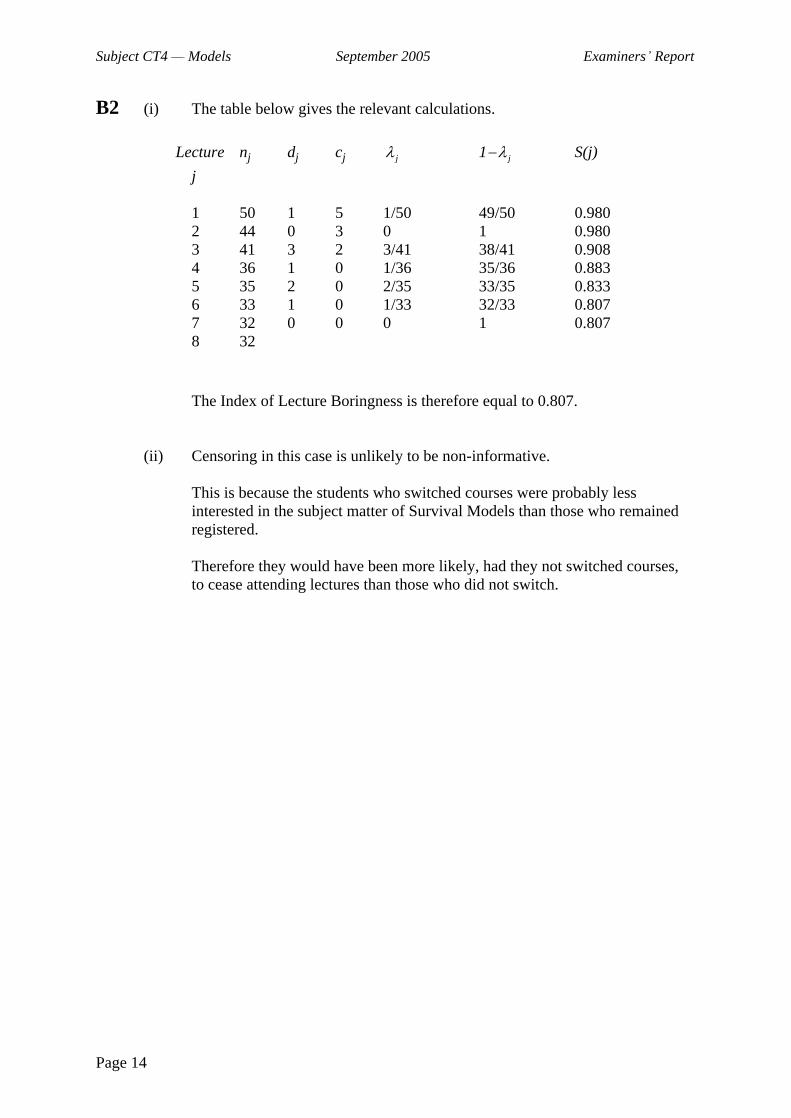
B2 (i) The table below gives the relevant calculations.
Lecture nj dj cj j
1 j
S(j)
j
1 50 1 5 1/50 49/50 0.980 2 44 0 3 0 1 0.980 3 41 3 2 3/41 38/41 0.908 4 36 1 0 1/36 35/36 0.883 5 35 2 0 2/35 33/35 0.833 6 33 1 0 1/33 32/33 0.807 7 32 0 0 0 1 0.807 8 32
The Index of Lecture Boringness is therefore equal to 0.807.
(ii) Censoring in this case is unlikely to be non-informative.
This is because the students who switched courses were probably less interested in the subject matter of Survival Models than those who remained registered.
Therefore they would have been more likely, had they not switched courses, to cease attending lectures than those who did not switch.
Subject CT4 Models September 2005 Examiners Report
Page 15
B3 (i) The classification of deaths implies a calendar year rate interval.
A person who dies will be aged x on the birthday in the calendar year of death, which implies that he or she will be aged x next birthday on 1 January in the calendar year of death.
Since 1 January is the start of the rate interval, the age range at the start is x 1 to x.
(ii) A census of those aged x next birthday on 1 January in each year would correspond to the classification of deaths.
But we have lives classified by age x last birthday.
However, the number alive aged x next birthday on any date is equal to the number alive aged x 1 last birthday.
The number alive aged x 1 last birthday on 1 January in year t is given by Px 1(t).
At the end of year t this cohort will be aged x last birthday.
Thus, using the trapezium rule, the correct exposed to risk at age x in year t is given by
11
( ) ( 1)2 x xP t P t .
Over the three calendar years 2002, 2003 and 2004, we have, therefore, exposed to risk =
1
1
1
1(2002) (2003)
21
(2003) (2004)2
1
(2004) (2005) .2
x x
x x
x x
P P
P P
P P
(iii) Assuming birthdays are uniformly distributed over the calendar year, the average age at the start of the rate interval will be x ½.
Therefore the average age in the middle of the rate interval is x.
Assuming a constant force of mortality between x ½ and x + ½, therefore, f = 0.
Subject CT4 Models September 2005 Examiners Report
Page 16
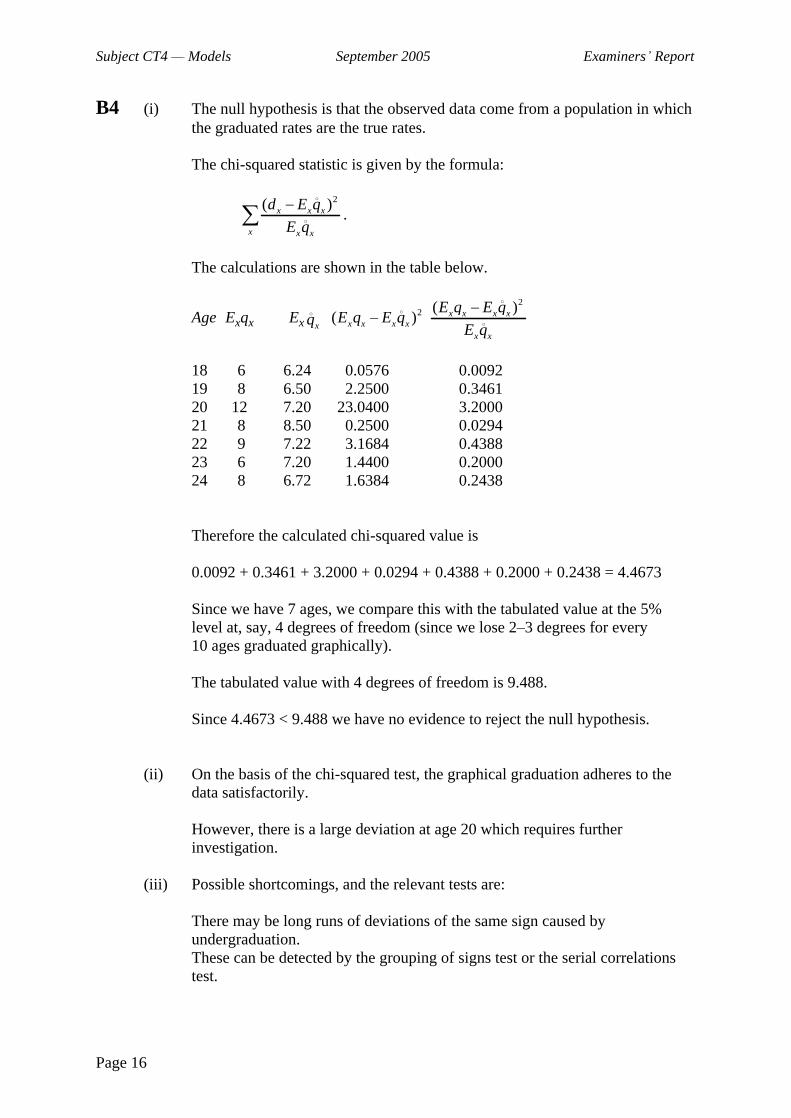
B4 (i) The null hypothesis is that the observed data come from a population in which the graduated rates are the true rates.
The chi-squared statistic is given by the formula:
2( )x x x
x x x
d E q
E q.
The calculations are shown in the table below.
Age Exqx Ex xq
2( )x x x xE q E q
2( )x x x x
x x
E q E q
E q
18 6 6.24 0.0576 0.0092 19 8 6.50 2.2500 0.3461 20 12 7.20 23.0400 3.2000 21 8 8.50 0.2500 0.0294 22 9 7.22 3.1684 0.4388 23 6 7.20 1.4400 0.2000 24 8 6.72 1.6384 0.2438
Therefore the calculated chi-squared value is
0.0092 + 0.3461 + 3.2000 + 0.0294 + 0.4388 + 0.2000 + 0.2438 = 4.4673
Since we have 7 ages, we compare this with the tabulated value at the 5% level at, say, 4 degrees of freedom (since we lose 2 3 degrees for every 10 ages graduated graphically).
The tabulated value with 4 degrees of freedom is 9.488.
Since 4.4673 < 9.488 we have no evidence to reject the null hypothesis.
(ii) On the basis of the chi-squared test, the graphical graduation adheres to the data satisfactorily.
However, there is a large deviation at age 20 which requires further investigation.
(iii) Possible shortcomings, and the relevant tests are:
There may be long runs of deviations of the same sign caused by undergraduation. These can be detected by the grouping of signs test or the serial correlations test.
Subject CT4 Models September 2005 Examiners Report
Page 17
There may be one or two large deviations at particular ages, balanced by lots of small deviations (as in the example in part (i)) These can be detected by the individual standardised deviations test.
The graduated rates may be too high or too low over the whole of the age range, but by an amount too small for the chi-squared test to detect. The signs test or the cumulative deviations test will detect this.
The results of the graduation may not be smooth. This can be detected by looking at the third order differences of the graduated rates xq . If the rates are smooth, these should be small in magnitude
compared with the quantities themselves and should progress regularly.
B5 (i) Taking logarithms of the Gompertz hazard produces
log x = log B + x log c
which indicates that the rate of increase of the hazard with age is constant.
Empirically, this is often a reasonable assumption for middle ages and older ages, which include the age range 50 65 years.
(ii) Putting B = exp( 0 + 1 X1 + 2 X2 + 3 X3) into the Gompertz model produces
x = exp( 0 + 1 X1 + 2 X2 + 3 X3) . cx,
defining x as duration since 50th birthday.
The hazard can therefore be factorised into two parts:
exp( 0 + 1 X1 + 2 X2 + 3 X3), which depends only on the values of the covariates, and
cx, which depends only on duration.
Therefore the ratio between the hazards for any two persons with different characteristics does not depend on duration, and so the model is a proportional hazards model.
(iii) (a) The baseline hazard in this model relates to
a female, non-smoker, who drinks less than 21 units of alcohol per week.
Subject CT4 Models September 2005 Examiners Report
Page 18
(b) For a female cigarette smoker who does not consume alcohol we have X1 = 0, X2 = 1, X3 = 0 and x = 5.
Therefore the hazard is given by
5 = exp( 0 + 1 .0 + 2 .1 + 3 .0) . c5
= exp( 5 + 0.75) 1.105
= 0.0230.
(c) The hazard for a non-smoker at duration u is given by the formula
u = exp( 0 + 1 X1 + 3 X3) . cu,
The hazard for a smoker at duration v is given by the formula
*v = exp( 0 + 1 X1 + 0.75 + 3 X3) . cv.
If the smoker s and non-smoker s hazards are the same, then
u = *v,
which implies that exp( 0 + 1 X1 + 3 X3).cu
= exp( 0 + 1 X1 + 0.75 + 3 X3) . cv.
which simplifies to cu = exp(0.75) . cv,
so that cu/cv = cu v = exp(0.75) = 2.117.
Since c = 1.1, we have 1.1u v = 2.117.
Therefore
u
v = log(2.117)/log(1.1) = 0.75/0.0953 = 7.87.
So when the two hazards are equal, the non-smoker is approximately eight years older than the smoker.
Alternatively this could be demonstrated by calculating u and *u-8
and showing that they are approximately the same.
Subject CT4 Models September 2005 Examiners Report
Page 19
B6 (i) Let the probability of failure within the first 20 days be 20 0q .
We have:
20 0 20 0 1 0 19 1
1 0
1 1 .
1 (1 )exp( 19 )
1 0.95exp( 19 0.01)
1 0.95exp( 0.19)
1 0.95(0.82696)
q p p p
q
which is 0.21439.
(ii) (a) The complete expectation of life of a one-day old light bulb, 1e is
given by
1 10
0.01
0
t
t
e p dt
e dt
Integrating, this gives
0.011
0
1 10 1
0.01 0.01te e
= 100 days.
(b) The complete expectation of life of a new light bulb, 0e is given by
1
0 0 0 00 0 1
t t te p dt p dt p dt . (*)
Alternative 1
Assume a uniform distribution of failure times between exact ages 0 and 1,
the first term in (*) is equal to
Subject CT4 Models September 2005 Examiners Report
Page 20
1 0
1 0
11
21
1 (1 )2
1(1 0.95) 0.975
2
p
q
The second term is equal to
1 0 10
0.95(100)tp p dt
(using the result from part (i) above).
Therefore:
0 0.975 100 0.95 95.975 days.e
Alternative 2
Assume a constant force of failure between exact ages 0 and 1
Let this constant force be .
Then 1
1 00
1 0
exp exp( )
1 0.95.
p ds
q
So that exp( ) 0.95
and log(0.95) 0.0513.
Thus the first term on the right-hand side of (*) is
Subject CT4 Models September 2005 Examiners Report
Page 21
1 1
00 0
10
exp( 0.0513 )
1exp( 0.0513 )
0.0513
1exp( 0.0513) 1
0.0513
0.97478,
t p dt t dt
t
and the second term is equal to
1 0 10
0.95(100)tp p dt
(using the result from part (i) above).
So that
0 0.97478 100 0.95 95.97478 days.e
(iii) The complete expectation of life of a light bulb at any age is an average of the future lifetimes of all bulbs which have not failed before that age.
The value of 0e is lower than 1e because the average 0e includes the very
short lifetimes of the relatively large proportion of bulbs which fail in the first
day, which deflate the average, whereas 1e excludes these.
END OF EXAMINERS REPORT

Faculty of Actuaries Institute of Actuaries
EXAMINATION
29 March 2006 (am)
Subject CT4 (103) Models (103 Part) Core Technical
Time allowed: One and a half hours
INSTRUCTIONS TO THE CANDIDATE
1. Enter all the candidate and examination details as requested on the front of your answer booklet.
2. You must not start writing your answers in the booklet until instructed to do so by the supervisor.
3. Mark allocations are shown in brackets.
4. Attempt all 6 questions, beginning your answer to each question on a separate sheet.
5. Candidates should show calculations where this is appropriate.
Graph paper is not required for this paper.
AT THE END OF THE EXAMINATION
Hand in BOTH your answer booklet, with any additional sheets firmly attached, and this question paper.
In addition to this paper you should have available the 2002 edition of the Formulae and Tables and your own electronic calculator.
Faculty of Actuaries CT4 (103) A2006 Institute of Actuaries
CT4 (103) A2006 2
A1 In the context of a stochastic process {Xt : t
J}, explain the meaning of the
following conditions:
(a) strict stationarity (b) weak stationarity
[3]
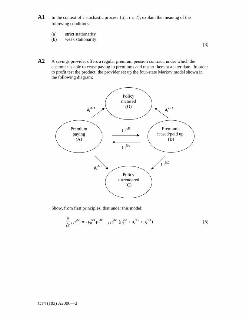
A2 A savings provider offers a regular premium pension contract, under which the customer is able to cease paying in premiums and restart them at a later date. In order to profit test the product, the provider set up the four-state Markov model shown in the following diagram:
Show, from first principles, that under this model:
0 0 0. .( )AB AA AB AB BA BC BDt t t t t t tp p p
t
[5]
tAB
tBC
tBA
tAC
tAD
tBD
Premium paying
(A)
Premiums ceased/paid up
(B)
Policy matured
(D)
Policy surrendered
(C)
CT4 (103) A2006 3 PLEASE TURN OVER
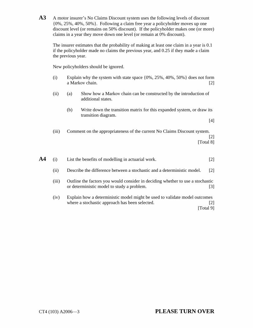
A3 A motor insurer s No Claims Discount system uses the following levels of discount {0%, 25%, 40%, 50%}. Following a claim free year a policyholder moves up one discount level (or remains on 50% discount). If the policyholder makes one (or more) claims in a year they move down one level (or remain at 0% discount).
The insurer estimates that the probability of making at least one claim in a year is 0.1 if the policyholder made no claims the previous year, and 0.25 if they made a claim the previous year.
New policyholders should be ignored.
(i) Explain why the system with state space {0%, 25%, 40%, 50%} does not form a Markov chain. [2]
(ii) (a) Show how a Markov chain can be constructed by the introduction of additional states.
(b) Write down the transition matrix for this expanded system, or draw its transition diagram.
[4]
(iii) Comment on the appropriateness of the current No Claims Discount system. [2]
[Total 8]
A4 (i) List the benefits of modelling in actuarial work. [2]
(ii) Describe the difference between a stochastic and a deterministic model. [2]
(iii) Outline the factors you would consider in deciding whether to use a stochastic or deterministic model to study a problem. [3]
(iv) Explain how a deterministic model might be used to validate model outcomes where a stochastic approach has been selected. [2]
[Total 9]
CT4 (103) A2006 4
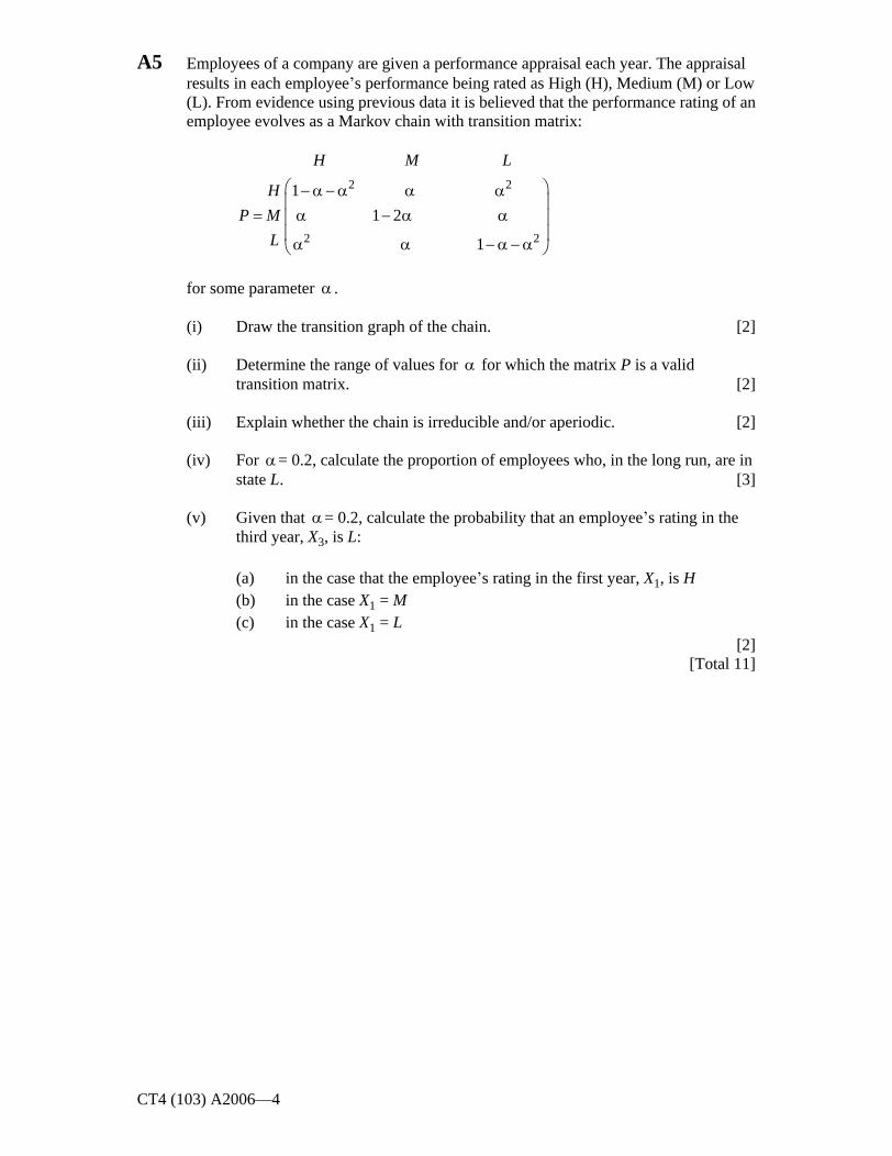
A5 Employees of a company are given a performance appraisal each year. The appraisal results in each employee s performance being rated as High (H), Medium (M) or Low (L). From evidence using previous data it is believed that the performance rating of an employee evolves as a Markov chain with transition matrix:
2 2
2 2
1
1 2
1
H M L
H
P M
L
for some parameter .
(i) Draw the transition graph of the chain. [2]
(ii) Determine the range of values for for which the matrix P is a valid transition matrix. [2]
(iii) Explain whether the chain is irreducible and/or aperiodic. [2]
(iv) For = 0.2, calculate the proportion of employees who, in the long run, are in state L. [3]
(v) Given that = 0.2, calculate the probability that an employee s rating in the third year, X3, is L:
(a) in the case that the employee s rating in the first year, X1, is H (b) in the case X1 = M (c) in the case X1 = L
[2] [Total 11]
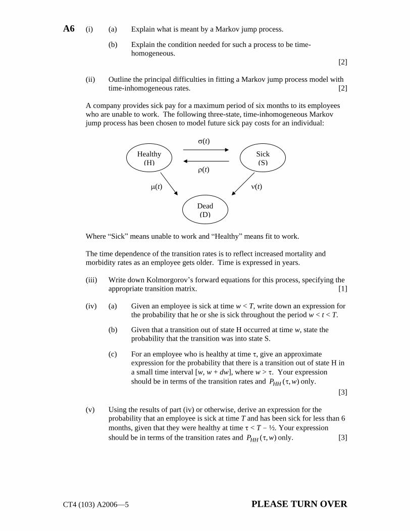
CT4 (103) A2006 5 PLEASE TURN OVER
A6 (i) (a) Explain what is meant by a Markov jump process.
(b) Explain the condition needed for such a process to be time-homogeneous.
[2]
(ii) Outline the principal difficulties in fitting a Markov jump process model with time-inhomogeneous rates. [2]
A company provides sick pay for a maximum period of six months to its employees who are unable to work. The following three-state, time-inhomogeneous Markov jump process has been chosen to model future sick pay costs for an individual:
Where Sick means unable to work and Healthy means fit to work.
The time dependence of the transition rates is to reflect increased mortality and morbidity rates as an employee gets older. Time is expressed in years.
(iii) Write down Kolmorgorov s forward equations for this process, specifying the appropriate transition matrix. [1]
(iv) (a) Given an employee is sick at time w < T, write down an expression for the probability that he or she is sick throughout the period w < t < T.
(b) Given that a transition out of state H occurred at time w, state the probability that the transition was into state S.
(c) For an employee who is healthy at time , give an approximate expression for the probability that there is a transition out of state H in a small time interval [w, w + dw], where w > . Your expression should be in terms of the transition rates and ( , )HHP w only.
[3]
(v) Using the results of part (iv) or otherwise, derive an expression for the probability that an employee is sick at time T and has been sick for less than 6 months, given that they were healthy at time
< T - ½. Your expression should be in terms of the transition rates and ( , )HHP w only. [3]
(t)
Healthy (H)
Sick (S)
Dead (D)
(t)
(t)
(t)

CT4 (103) A2006 6
(vi) Comment on the suggestions that:
(a) (t) should also depend on the holding time in state S, and (b) mortality rates can be ignored.
[3] [Total 14]
END OF PAPER

Faculty of Actuaries Institute of Actuaries
EXAMINATION
29 March 2006 (am)
Subject CT4 (104) Models (104 Part) Core Technical
Time allowed: One and a half hours
INSTRUCTIONS TO THE CANDIDATE
1. Enter all the candidate and examination details as requested on the front of your answer booklet.
2. You must not start writing your answers in the booklet until instructed to do so by the supervisor.
3. Mark allocations are shown in brackets.
4. Attempt all 6 questions, beginning your answer to each question on a separate sheet.
5. Candidates should show calculations where this is appropriate.
Graph paper is not required for this paper.
AT THE END OF THE EXAMINATION
Hand in BOTH your answer booklet, with any additional sheets firmly attached, and this question paper.
In addition to this paper you should have available the 2002 edition of the Formulae and Tables and your own electronic calculator.
Faculty of Actuaries CT4 (104) A2006 Institute of Actuaries

CT4 (104) A2006 2
B1 A Cox proportional hazards model was estimated to assess the effect on survival of a person s sex and his or her self-esteem (measured on a three-point scale as low , medium or high ). The baseline category was males with low self-esteem.
Write down the equation of the model, using algebraic symbols to represent variables and parameters and defining all the symbols that you use. [4]
B2 (i) (a) Explain why it is important to sub-divide data when carrying out mortality investigations.
(b) Describe the problems that can arise with sub-dividing data. [4]
(ii) List four factors which are often used to sub-divide life assurance data. [2] [Total 6]
B3 (i) Assume that the force of mortality between consecutive integer ages, y and y + 1, is constant and takes the value µy.
Let Tx be the future lifetime after age x ( x y ) and Sx(t) be the survival function of Tx.
Show that:
log[ ( )] log[ ( 1 )]y x xS y x S y x . [4]
(ii) An investigation was carried out into the mortality of male life office policyholders. Each life was observed from his 50th birthday until the first of three possible events occurred: his 55th birthday, his death, or the lapsing of his policy. For those policyholders who died or allowed their policies to lapse, the exact age at exit was recorded.
Using the result from part (i) or otherwise, describe how the data arising from this investigation could be used to estimate:
(a) 50
(b) 5 50q
[3] [Total 7]

CT4 (104) A2006 3 PLEASE TURN OVER
B4 A company is interested in estimating policy lapse rates by age. It conducts an investigation into this, which lasts for the whole of the calendar year 2003. The investigation collects the following data for a sample of policies which are funded by annual premiums:
the age last birthday of the policyholder when the policy was taken out;
the number of premiums the policyholder paid before the policy lapsed.
In addition, the number of policies in-force on 1 January each year is available,
classified by age x last birthday and years t elapsed since 1 January 2003, *,( )x tP .
(i) State the rate interval in this investigation. [1]
(ii) Derive an expression for the exposed-to-risk in terms of *,x tP , stating any
assumptions you make. [7]
(iii) Comment on the reasonableness or otherwise of the assumptions you made in your answer to part (ii). [2]
[Total 10]
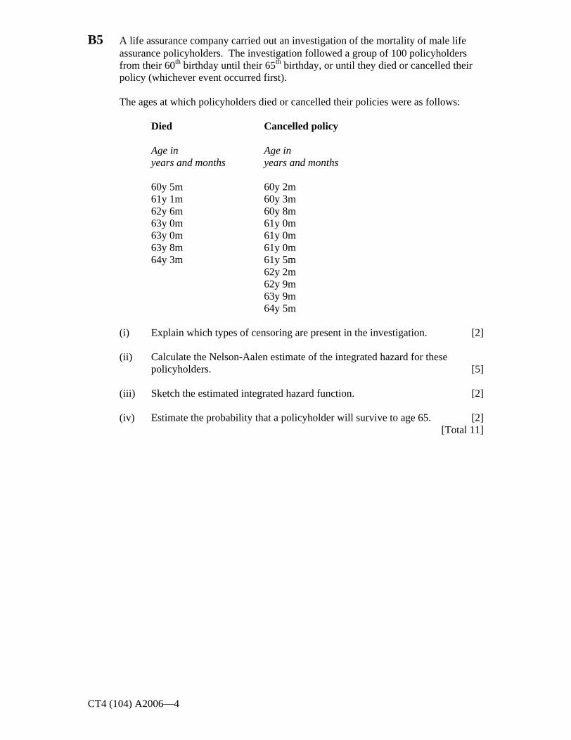
CT4 (104) A2006 4
B5 A life assurance company carried out an investigation of the mortality of male life assurance policyholders. The investigation followed a group of 100 policyholders from their 60th birthday until their 65th birthday, or until they died or cancelled their policy (whichever event occurred first).
The ages at which policyholders died or cancelled their policies were as follows:
Died
Age in years and months
Cancelled policy
Age in years and months
60y 5m 61y 1m 62y 6m 63y 0m 63y 0m 63y 8m 64y 3m
60y 2m 60y 3m 60y 8m 61y 0m 61y 0m 61y 0m 61y 5m 62y 2m 62y 9m 63y 9m 64y 5m
(i) Explain which types of censoring are present in the investigation. [2]
(ii) Calculate the Nelson-Aalen estimate of the integrated hazard for these policyholders. [5]
(iii) Sketch the estimated integrated hazard function. [2]
(iv) Estimate the probability that a policyholder will survive to age 65. [2] [Total 11]
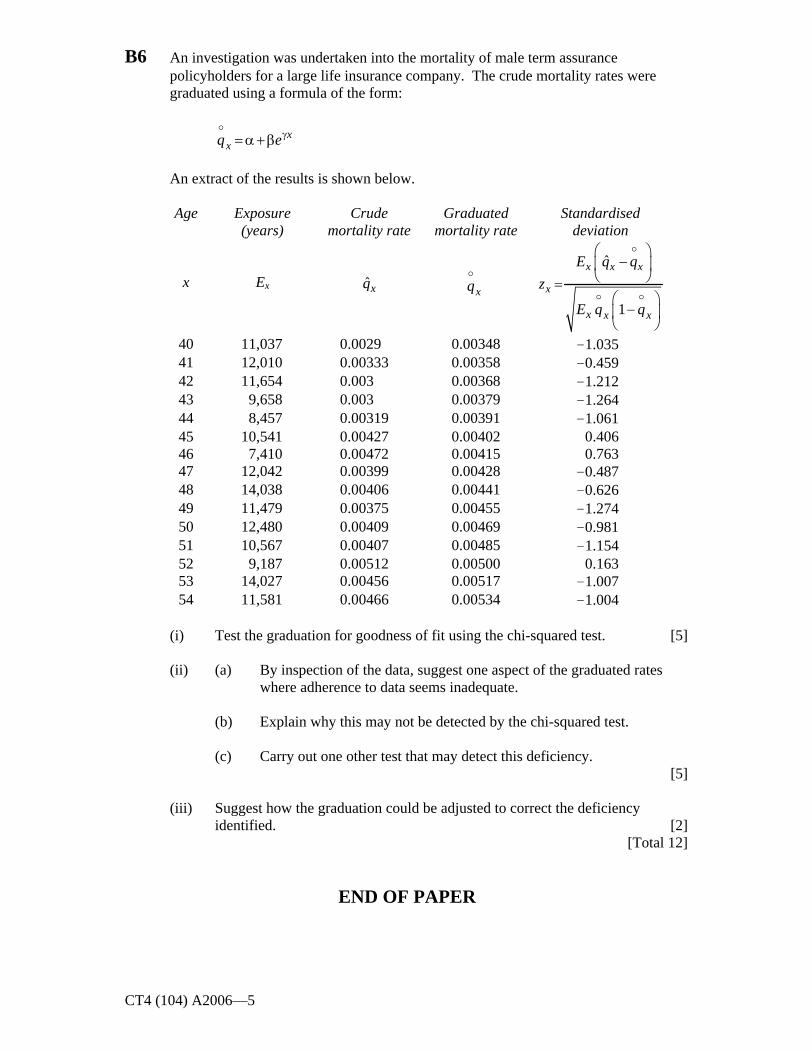
CT4 (104) A2006 5
B6 An investigation was undertaken into the mortality of male term assurance policyholders for a large life insurance company. The crude mortality rates were graduated using a formula of the form:
xxq e
An extract of the results is shown below.
Age Exposure (years)
Crude mortality rate
Graduated mortality rate
Standardised deviation
x Ex xq
xq
1
x x x
x
x x x
E q q
z
E q q
40 11,037 0.0029 0.00348 -1.035 41 12,010 0.00333 0.00358 -0.459 42 11,654 0.003 0.00368 -1.212 43 9,658 0.003 0.00379 -1.264 44 8,457 0.00319 0.00391 -1.061 45 10,541 0.00427 0.00402 0.406 46 7,410 0.00472 0.00415 0.763 47 12,042 0.00399 0.00428 -0.487 48 14,038 0.00406 0.00441 -0.626 49 11,479 0.00375 0.00455 -1.274 50 12,480 0.00409 0.00469 -0.981 51 10,567 0.00407 0.00485 -1.154 52 9,187 0.00512 0.00500 0.163 53 14,027 0.00456 0.00517 -1.007 54 11,581 0.00466 0.00534 -1.004
(i) Test the graduation for goodness of fit using the chi-squared test. [5]
(ii) (a) By inspection of the data, suggest one aspect of the graduated rates where adherence to data seems inadequate.
(b) Explain why this may not be detected by the chi-squared test.
(c) Carry out one other test that may detect this deficiency. [5]
(iii) Suggest how the graduation could be adjusted to correct the deficiency identified. [2]
[Total 12]
END OF PAPER

Faculty of Actuaries Institute of Actuaries
EXAMINATION
April 2006
Subject CT4 Models (includes both 103 and 104 parts) Core Technical
EXAMINERS REPORT
Introduction
The attached subject report has been written by the Principal Examiner with the aim of helping candidates. The questions and comments are based around Core Reading as the interpretation of the syllabus to which the examiners are working. They have however given credit for any alternative approach or interpretation which they consider to be reasonable.
M Flaherty Chairman of the Board of Examiners
June 2006
Faculty of Actuaries Institute of Actuaries

Subject CT4 Models Core Technical April 2006
Examiners Report
Page 2
Comments
Comments on solutions presented to individual questions for this April 2006 paper are given below.
103 Part
Question A1 This was well answered overall. Most candidates scored better on part (b); marks were lost on part (a) because answers were imprecise.
Question A2 This was reasonably well answered overall. Marks were lost because candidates did not show sufficient steps.
Question A3 This was reasonably well answered overall In part (ii), many candidates included more states than required. (See end of solution for further comments.)
Question A4 This was poorly answered. Very few candidates scored highly on this question. Most failed to provide sufficient, distinct points.
Question A5 This was very well answered. Marks were lost on part (ii) when candidates failed to consider all the conditions applying, and part (v) where many candidates calculated P3.
Question A6 This was poorly answered, although the better candidates did manage to score highly.
104 Part|
Question B1 This was well answered overall. The most common mistake was to use only one variable for self-esteem.
Question B2 This was reasonably well answered overall. In part (i), many candidates discussed premium setting and anti-selection, which was not relevant to the question asked.
Question B3 This was very poorly answered, with very few candidates scoring highly. Some alternative approaches to part (i) received credit, although care was needed over the ranges fro which x was constant. Most candidates
attempted part (ii), although few used the solution to part (i).
Question B4 This was very poorly answered. Most solutions offered lacked a coherent explanation.
Question B5 This was very well answered. Marks were most frequently lost in part (i), because of insufficient explanation of the types of censoring present.
Question B6 This was reasonably well answered overall. In part (ii), many candidates carried out a signs test. The use of the Normal approximation to the Binomial was not acceptable in this case, and candidates who used this lost marks. (See end of solution (ii)(c) for further comments.)
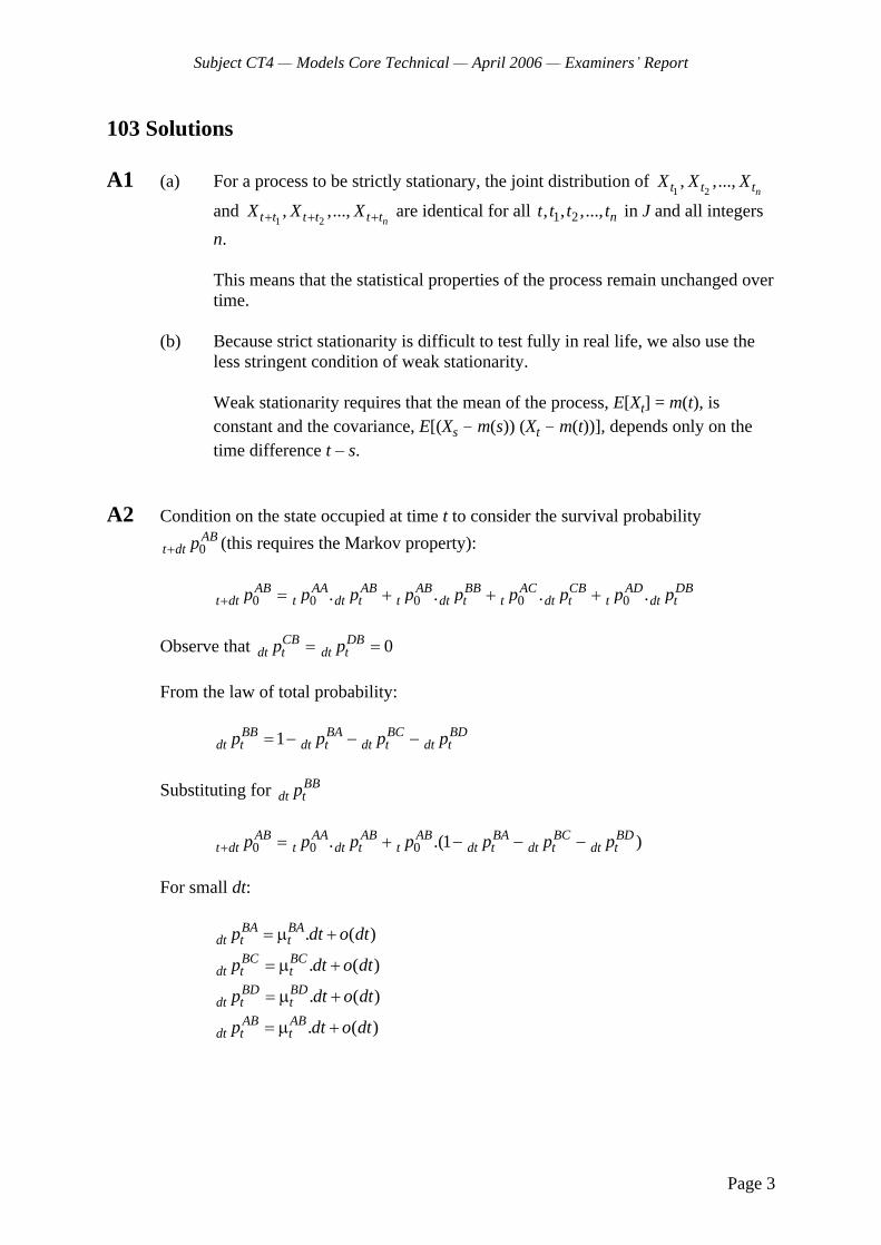
Subject CT4 Models Core Technical April 2006
Examiners Report
Page 3
103 Solutions
A1 (a) For a process to be strictly stationary, the joint distribution of 1 2, ,...,
nt t tX X X
and
1 2, ,...,
nt t t t t tX X X are identical for all 1 2, , ,..., nt t t t in J and all integers
n.
This means that the statistical properties of the process remain unchanged over time.
(b) Because strict stationarity is difficult to test fully in real life, we also use the less stringent condition of weak stationarity.
Weak stationarity requires that the mean of the process, E[Xt] = m(t), is constant and the covariance, E[(Xs - m(s)) (Xt - m(t))], depends only on the time difference t
s.
A2 Condition on the state occupied at time t to consider the survival probability
0AB
t dt p (this requires the Markov property):
0 0 0 0 0. . . .AB AA AB AB BB AC CB AD DBt dt t dt t t dt t t dt t t dt tp p p p p p p p p
Observe that 0CB DBdt t dt tp p
From the law of total probability:
1BB BA BC BDdt t dt t dt t dt tp p p p
Substituting for BBdt tp
0 0 0. .(1 )AB AA AB AB BA BC BDt dt t dt t t dt t dt t dt tp p p p p p p
For small dt:
. ( )BA BAdt t tp dt o dt
. ( )BC BCdt t tp dt o dt
. ( )BD BDdt t tp dt o dt
. ( )AB ABdt t tp dt o dt

Subject CT4 Models Core Technical April 2006
Examiners Report
Page 4
Where o(dt) covers the possibility of more than one transition in time dt and
lim ( )0
0
o dt
dt dt
Substituting in:
0 0 0. . (1 . . . ) ( )AB AA AB AB BA BC BDt dt t t t t t tp p dt p dt dt dt o dt
0 00 0 0
lim. ( )
0
AB ABAB AA AB AB BA BC BDt dt t
t t t t t t tp p
p p pt dtdt
A3 (i) This is not a Markov chain because it does not possess the Markov property, that is transition probabilities do not depend only on the current state.
Specifically, if you are in the 25% discount level, the transition probability to state 0% is 0.25 if a claim was made last year and 0.1 if the previous year was claim free.
(ii) (a) Split the 25% and 40% discount states to include whether the previous year was claim free.
New state space:
0% discount 25%NC (no claim last year) 25%C (at least one claim last year) 40%NC (no claim last year) 40%C (at least one claim last year) 50%

Subject CT4 Models Core Technical April 2006
Examiners Report
Page 5
(b)
0.1
0.75
0.75
0%
25% NC
40% NC
50%
25% C
40% C
0.9 0.25
0.25
0.25
0.1
0.1
0.75
0.9
0.9
New state
0% 25%C 25%NC 40%C 40%NC 50% 0% 0.25 0 0.75 0 0 0 25%C 0.25 0 0 0 0.75 0 25%NC 0.1 0 0 0 0.9 0 40%C 0 0.25 0 0 0 0.75 40%NC 0 0.1 0 0 0 0.9
Old
Sta
te
50% 0 0 0 0.1 0 0.9
(iii) In theory, the insurer should just use 2 NCD states according to whether the policyholder made a claim in the previous year. This is because the company believes the claims frequency is the same for drivers who have not made a claim for 1, 2, 3 years (i.e. it remains at 0.1 whether the driver has been claims-free for 1 or 10 years).
However there may be other reasons for adopting this scale:
Marketing or competitive pressures.
It may discourage the policyholder from making small claims, or encourage careful driving, to preserve their discount.
General comments:
The following, more general comments about the appropriateness of an NCD model also received credit:
It is appropriate to award a no-claims discount because there is empirical evidence that drivers who have made a recent claim are more likely to make a further claim.
More factors should be taken into account (with a suitable example such as how long the policyholder has been driving).

Subject CT4 Models Core Technical April 2006
Examiners Report
Page 6
A4 (i) Systems with long time frames such as the operation of a pension fund can be studied in compressed time.
Different future policies or possible actions can be compared to see which best suits the requirements or constraints of a user.
Complex situations can be studied.
Modelling may be the only practicable approach for certain actuarial problems.
(ii) A model is described as stochastic if it allows for the random variation in at least one input variable.
Often the output from a stochastic model is in the form of many simulated possible outcomes of a process, so distributions can be studied.
A deterministic model can be thought of as a special case of a stochastic model where only a single outcome from the underlying random processes is considered.
Sometimes stochastic models have analytical/closed form solutions, such that simulation is not required, but they are still stochastic as they allow for factors to be random variables.
(iii)
If the distribution of possible outcomes is required then stochastic modelling would be needed, or if only interested in a single scenario then deterministic.
Budget and time available stochastic modelling can be considerably more expensive and time consuming.
Nature of existing models.
Audience for the results and the way they will be communicated.
The following factors may favour a stochastic approach:
The regulator may require a stochastic approach.
Extent of non-linear variation for example existence of options or guarantees.
Skewness of distribution of underlying variables, such as cost of storm claims.
Interaction between variables, such as lapse rates with investment performance.
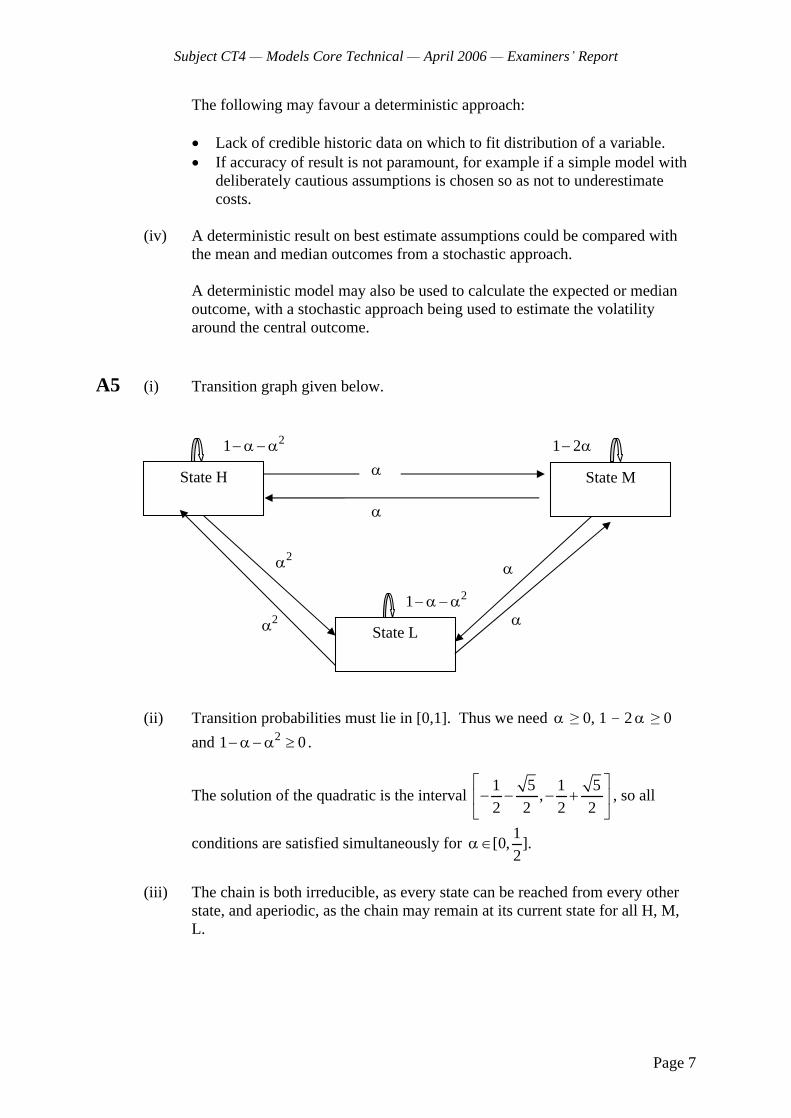
Subject CT4 Models Core Technical April 2006
Examiners Report
Page 7
The following may favour a deterministic approach:
Lack of credible historic data on which to fit distribution of a variable.
If accuracy of result is not paramount, for example if a simple model with deliberately cautious assumptions is chosen so as not to underestimate costs.
(iv) A deterministic result on best estimate assumptions could be compared with the mean and median outcomes from a stochastic approach.
A deterministic model may also be used to calculate the expected or median outcome, with a stochastic approach being used to estimate the volatility around the central outcome.
A5 (i) Transition graph given below.
(ii) Transition probabilities must lie in [0,1]. Thus we need
0, 1 - 2
0
and 21 0 .
The solution of the quadratic is the interval 1 5 1 5
,2 2 2 2
, so all
conditions are satisfied simultaneously for 1
[0, ].2
(iii) The chain is both irreducible, as every state can be reached from every other state, and aperiodic, as the chain may remain at its current state for all H, M, L.
2
2
State H
State L
State M
21
1 2
21
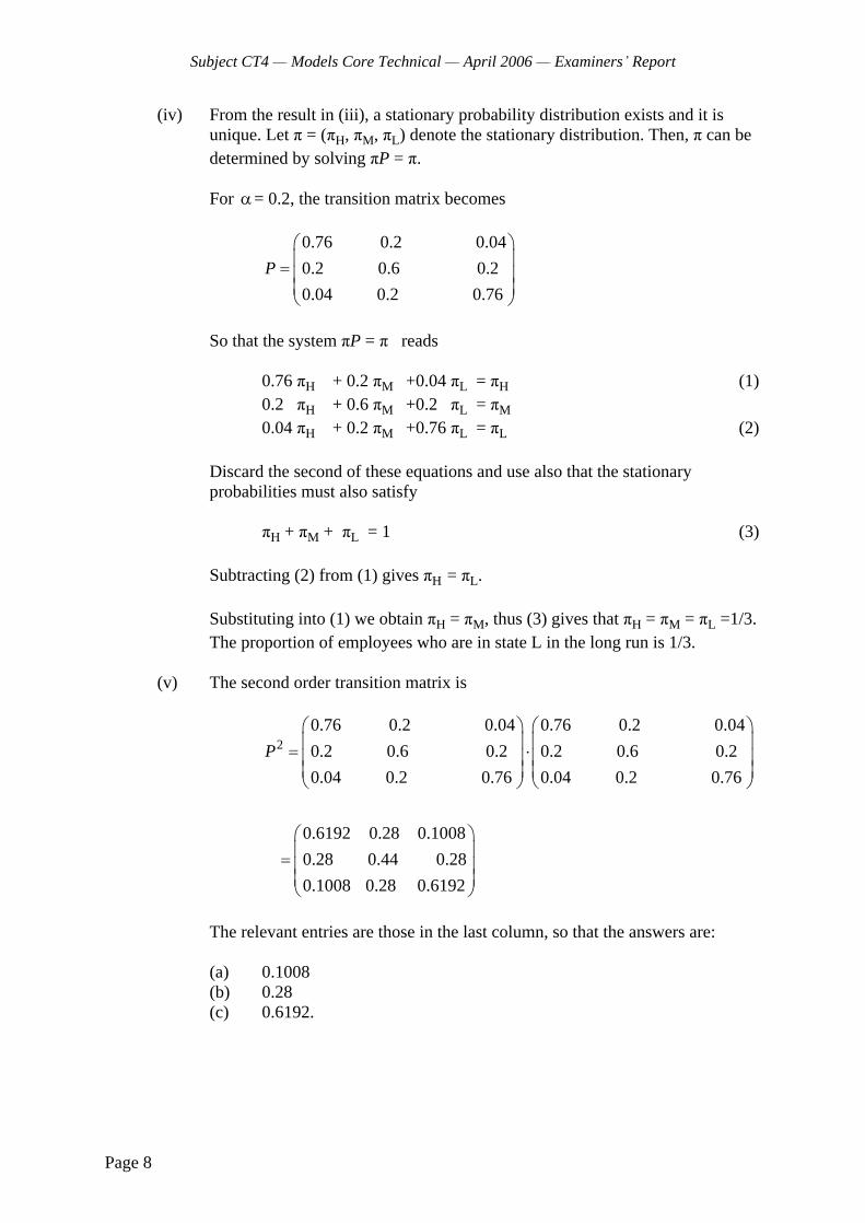
Subject CT4 Models Core Technical April 2006
Examiners Report
Page 8
(iv) From the result in (iii), a stationary probability distribution exists and it is unique. Let = ( H, M, L) denote the stationary distribution. Then, can be determined by solving P = .
For = 0.2, the transition matrix becomes
0.76 0.2 0.04
0.2 0.6 0.2
0.04 0.2 0.76
P
So that the system P = reads
0.76 H + 0.2 M +0.04 L = H (1) 0.2 H + 0.6 M +0.2 L = M
0.04 H + 0.2 M +0.76 L = L (2)
Discard the second of these equations and use also that the stationary probabilities must also satisfy
H + M + L = 1 (3)
Subtracting (2) from (1) gives H = L.
Substituting into (1) we obtain H = M, thus (3) gives that H = M = L =1/3. The proportion of employees who are in state L in the long run is 1/3.
(v) The second order transition matrix is
2
0.76 0.2 0.04 0.76 0.2 0.04
0.2 0.6 0.2 0.2 0.6 0.2
0.04 0.2 0.76 0.04 0.2 0.76
0.6192 0.28 0.1008
0.28 0.44 0.28
0.1008 0.28 0.6192
P
The relevant entries are those in the last column, so that the answers are:
(a) 0.1008 (b) 0.28 (c) 0.6192.
Subject CT4 Models Core Technical April 2006
Examiners Report
Page 9
A6 (i) (a) A continuous-time Markov process 0, tX t with a discrete state
space S is called a Markov jump process.
(b) In the case where the probabilities iXjXP st | for i, j in S and
ts0 depend only on the length of time interval st , the process is called time-homogeneous.
(ii) A model with time-inhomogeneous rates has more parameters, and there may not be sufficient data available to estimate these parameters.
Also, the solution to Kolmogorov s equations may not be easy (or even possible) to find analytically.
(iii) ( ) ( ). ( )P t P t A t
where
( ) ( ) ( ) ( )
( ) ( ) ( ) ( ) ( )
0 0 0
t t t t
A t t t t t
(iv) (a) Pr(Waiting time ) exp ( ( ) ( ))T
w
w
T w X S t t dt
(b) Given there is a transition from state H at time w, the probabilities that this is into state S or D are given by the relative transition rates at time w.
So Probability into state S = ( )
( ) ( )
w
w w
(c) This is the probability that the individual is in state H at time w, multiplied by the sum of transition rates out of state H at time w, that is:
( , ).( ( ) ( ))HHP w w w dw
Subject CT4 Models Core Technical April 2006
Examiners Report
Page 10
(v) Expressing time in years,
Pr( ,Waiting time 1/ 2 )TX S X H
1/ 2
Pr(Transition fromstate H at ) Pr(Transition toS) Pr(stays inS to timeT)T
T
w dW
= 1/ 2
( )( , ).( ( ) ( )). .exp ( ( ) ( )) .
( ) ( )
T T
HHT w
wP w w w t t dt dw
w w
=1/ 2
( , ). ( ).exp ( ( ) ( )) .T T
HHT w
P w w t t dt dw
(vi) (a) This is likely to improve the predictive power of the model because:
There is empirical evidence that recovery rates depend on the duration of the sickness.
The limit of 6 months on sick pay may cause some durational effects around this point.
However this would make the model more complicated to analyse, and increase the volume of data required to fit parameters reliably.
(b) For individuals in employment mortality rates are likely to be low, and may be ignorable. It is less likely that mortality out of state S could be excluded.

Subject CT4 Models Core Technical April 2006
Examiners Report
Page 11
104 Solutions
B1 0 1 2 3( ) ( ) exp[ ]h t h t F M H
where
( )h t is the estimated hazard,
0 ( )h t is the baseline hazard,
F is a variable taking the value 1 if the life is female, and 0 otherwise,
M is a variable taking the value 1 if the life has medium self- esteem and 0 otherwise,
H is a variable taking the value 1 if the life has high self-esteem and 0 otherwise, and
1 2 3, and are parameters to be estimated.
B2 (i) (a) The models of mortality we use assume that we can observe a group of lives with the same mortality characteristics. This is not possible in practice.
However, data can be sub-divided according to certain characteristics that we know to have a significant effect on mortality.
This will reduce the heterogeneity of each group, so that we can at least observe groups with similar, but not the same, characteristics.
(b) Sub-dividing data using many factors can result in the numbers in each class being too low.
It is necessary to strike a balance between homogeneity of the group and retaining a large enough group to make statistical analysis possible.
Sufficient data may not be collected to allow sub-division.
This may be because marketing pressures mean proposal forms are kept to a minimum.
Subject CT4 Models Core Technical April 2006
Examiners Report
Page 12
(ii) The following are factors often used:
Sex Age Type of policy Smoker/Non-smoker status Level of underwriting Duration in force Sales channel Policy size Occupation (or social class) of policyholder Known impairments Geographical region
B3 (i) Consider the year of age between y and y + 1. We know that
0
expt
t y y sp ds .
If t=1 and y s y (a constant), evaluating the integral produces
expy yp .
Now, conditioning on survival to age x, survival to age y + 1 implies survival from age x to age y and then survival for a further year:
1 .y x x y y x xp p p .
Thus
1y x xy
y x x
pp
p,
which, since, in general ( )t x xp S t , may be written
( 1 )
( )x
yx
S y xp
S y x.
Subject CT4 Models Core Technical April 2006
Examiners Report
Page 13
Therefore
( 1 )exp( )
( )x
yx
S y x
S y x,
so that
( )log log[ ( )] log[ ( 1 )]
( 1 )x
y x xx
S y xS y x S y x
S y x.
(ii) (a) Using the result from part (i) and putting x = 50, y = 50 gives
5050 50
50
(0)log log[ (1)]
(1)
SS
S
Since we have censored data, because of the possibility of policy lapse, we should estimate 50 (1)S using the Kaplan-Meier or Nelson-Aalen
estimator and hence obtain an estimate of 50 .
(b) 5 50q = 1 - 5 50p ,
and, since
5 50 50(5)p S ,
5 50q can be estimated directly as 1
S50(5),
where S50(5) is the Kaplan-Meier or Nelson-Aalen estimator of the probability of a life aged 50 years surviving for a further 5 years.
B4 (i) We have a policy-year rate interval.
(ii) The age classification of the lapsing data is age last birthday on the policy anniversary prior to lapsing .
This can be calculated by adding the policyholder s age last birthday when the policy was taken to out to the number of annual premiums paid minus 1 (assuming that the first premium was paid at policy inception).
Define ,x tP
as the number of policies in force aged x last birthday at the
preceding policy anniversary at time t. This corresponds with the lapsing data.
Subject CT4 Models Core Technical April 2006
Examiners Report
Page 14
Then, if t is measured in years since 1 January 2003, a consistent exposed-to-risk would be
1
,0
cx x tE P dt ,
which, assuming that policy anniversaries are uniformly distributed across the calendar year,
may be approximated as
,0 ,11
[ ]2
cx x xE P P .
But we do not observe Px,t directly. Instead we observe *,x tP the number of
policies in force at time t, classified by age last birthday at time t.
But the range of exact ages that could apply to a life aged x last birthday on the policy anniversary prior to lapsing is (x, x + 2).
Assuming that birthdays are uniformly distributed across the policy year, half of these lives will be aged x last birthday and half will be aged x+ 1 last birthday.
Hence,
* *, , 1,
1[ ]
2x t x t x tP P P .
Therefore, by substituting this into the approximation above, the appropriate exposed-to-risk is
* * * *,0 1,0 ,1 1,1
1 1 1[ ] [ ] .
2 2 2cx x x x xE P P P P
(iii) Both assumptions might be unreasonable because:
policies might be taken out in large numbers just before the end of the tax year,
policies might tend to be taken out just before birthdays,
under group schemes, many policy anniversaries might be identical.
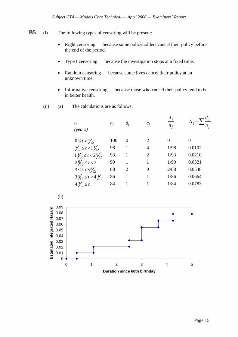
Subject CT4 Models Core Technical April 2006
Examiners Report
Page 15
B5 (i) The following types of censoring will be present:
Right censoring because some policyholders cancel their policy before the end of the period.
Type I censoring because the investigation stops at a fixed time.
Random censoring because some lives cancel their policy at an unknown time.
Informative censoring because those who cancel their policy tend to be in better health.
(ii) (a) The calculations are as follows:
tj (years)
nj dj cj
j
j
d
n
jj
j
d
n
5120 t
100 0 2 0 0 5 1
12 121t
98 1 4 1/98 0.0102 61
12 121 2t
93 1 2 1/93 0.0210 6
122 3t
90 1 1 1/90 0.0321 8
123 3t
88 2 0 2/88 0.0548 8 3
12 123 4t
86 1 1 1/86 0.0664 3
124 t
84 1 1 1/84 0.0783
(b)
00.010.020.030.040.050.060.070.080.09
0 1 2 3 4 5
Duration since 60th birthday
Est
imat
ed In
teg
rate
d H
azar
d
Subject CT4 Models Core Technical April 2006
Examiners Report
Page 16
(iii) Either
Using the results of the calculation in (ii), the survival function can be estimated by exp tS t .
And so, for t 4 3/12, we have
exp 0.0783 0.925S t
which is the probability of survival to 65.
Or
Using the Kaplan-Meier estimate of 1j
j
jt t
dS t
n,
we get, for t 4 3/12:
1 1 1 2 1 11 1 1 1 1 1
98 93 90 88 86 84S t
= 0.9243
B6 (i) The null hypothesis is that the crude rates come from a population in which true underlying rates are the graduated rates.
The test statistic is 2x
x
X z
Under the null hypothesis X has a 2 distribution with m degrees of freedom, where m is the number of age groups less one for each parameter fitted. So in
this case m = 15 3 = 12, ie 212X
The observed value of X is 12.816.
The critical value of the 212 distribution at the 5% level is 21.03
This is greater than the observed value of X
and so we have insufficient evidence to reject the null hypothesis.
Subject CT4 Models Core Technical April 2006
Examiners Report
Page 17
(ii) (a) The obvious problem with the graduation is one of overall bias. The graduated rates are consistently too high, resulting in too many negative deviations.
(b) This is not detected by the 2 test because the test statistic is the sum of the squared deviations and so information on the sign and some
information on the size of the individual deviations is lost. The 2 test would detect large bias, but in this case the graduated and crude rates are close enough that the statistic is below the critical value.
(c) Signs test
Let P be the number of positive deviations.
Under the null hypothesis, Binomial 15,0.5P .
We have 3 positive deviations. The probability of getting 3 or fewer positive signs (if the null hypothesis is true) is:
15 15 15 15 1510 1 2 32
151
1 15 105 4552
= 0.0176
This is less than 0.025 (this is a two-tailed test)
and so we reject the null hypothesis.
Cumulative deviations test
Our test statistic is
1
x x x xx
x x xx
E q E q
E q q
Under the null hypothesis, this has Normal(0, 1) distribution.
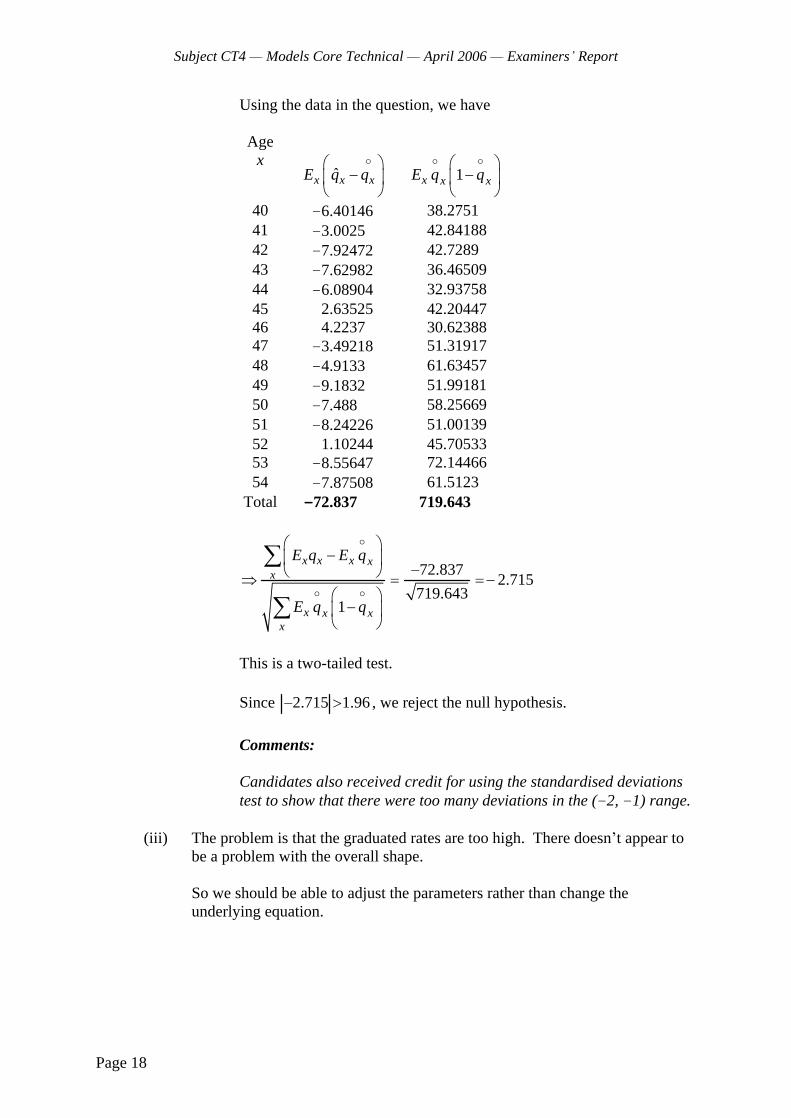
Subject CT4 Models Core Technical April 2006
Examiners Report
Page 18
Using the data in the question, we have
Age x
x x xE q q
1x x xE q q
40 -6.40146 38.2751 41 -3.0025 42.84188 42 -7.92472 42.7289 43 -7.62982 36.46509 44 -6.08904 32.93758 45 2.63525 42.20447 46 4.2237 30.62388 47 -3.49218 51.31917 48 -4.9133 61.63457 49 -9.1832 51.99181 50 -7.488 58.25669 51 -8.24226 51.00139 52 1.10244 45.70533 53 -8.55647 72.14466 54 -7.87508 61.5123
Total -72.837 719.643
72.8372.715
719.6431
x x x xx
x x xx
E q E q
E q q
This is a two-tailed test.
Since 2.715 1.96 , we reject the null hypothesis.
Comments:
Candidates also received credit for using the standardised deviations test to show that there were too many deviations in the (-2, -1) range.
(iii) The problem is that the graduated rates are too high. There doesn t appear to be a problem with the overall shape.
So we should be able to adjust the parameters rather than change the underlying equation.

Subject CT4 Models Core Technical April 2006
Examiners Report
Page 19
The problem persists across the whole age range, so the first adjustment to try would be to decrease the value of .
END OF EXAMINERS REPORT

Faculty of Actuaries Institute of Actuaries
EXAMINATION
6 September 2006 (am)
Subject CT4 (103) Models (103 Part) Core Technical
Time allowed: One and a half hours
INSTRUCTIONS TO THE CANDIDATE
1. Enter all the candidate and examination details as requested on the front of your answer booklet.
2. You must not start writing your answers in the booklet until instructed to do so by the supervisor.
3. Mark allocations are shown in brackets.
4. Attempt all 6 questions, beginning your answer to each question on a separate sheet.
5. Candidates should show calculations where this is appropriate.
Graph paper is not required for this paper.
AT THE END OF THE EXAMINATION
Hand in BOTH your answer booklet, with any additional sheets firmly attached, and this question paper.
In addition to this paper you should have available the 2002 edition of the Formulae and Tables and your own electronic calculator.
Faculty of Actuaries CT4 (103) S2006 Institute of Actuaries
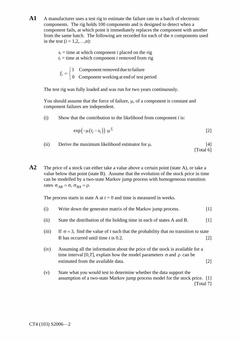
CT4 (103) S2006 2
A1 A manufacturer uses a test rig to estimate the failure rate in a batch of electronic components. The rig holds 100 components and is designed to detect when a component fails, at which point it immediately replaces the component with another from the same batch. The following are recorded for each of the n components used in the test (i = 1,2, ,n):
si = time at which component i placed on the rig ti = time at which component i removed from rig
1 Component removed due to failure
0 Component working at end of test periodif
The test rig was fully loaded and was run for two years continuously.
You should assume that the force of failure, , of a component is constant and component failures are independent.
(i) Show that the contribution to the likelihood from component i is:
exp ifi it s
[2]
(ii) Derive the maximum likelihood estimator for . [4] [Total 6]
A2 The price of a stock can either take a value above a certain point (state A), or take a value below that point (state B). Assume that the evolution of the stock price in time can be modelled by a two-state Markov jump process with homogeneous transition rates ,AB .BA
The process starts in state A at t = 0 and time is measured in weeks.
(i) Write down the generator matrix of the Markov jump process. [1]
(ii) State the distribution of the holding time in each of states A and B. [1]
(iii) If 3, find the value of t such that the probability that no transition to state B has occurred until time t is 0.2. [2]
(iv) Assuming all the information about the price of the stock is available for a time interval [0,T], explain how the model parameters and can be estimated from the available data. [2]
(v) State what you would test to determine whether the data support the assumption of a two-state Markov jump process model for the stock price. [1]
[Total 7]

CT4 (103) S2006 3 PLEASE TURN OVER
A3 (i) Define the following types of a stochastic process:
(a) a Poisson process (b) a compound Poisson process; and (c) a general random walk
[3]
(ii) For each of the processes in (i), state whether it operates in continuous or discrete time and whether it has a continuous or discrete state space. [2]
(iii) For each of the processes in (i), describe one practical situation in which an actuary could use such a process to model a real world phenomenon. [3]
[Total 8]
A4 The credit-worthiness of debt issued by companies is assessed at the end of each year by a credit rating agency. The ratings are A (the most credit-worthy), B and D (debt defaulted). Historic evidence supports the view that the credit rating of a debt can be modelled as a Markov chain with one-year transition matrix
0.92 0.05 0.03
0.05 0.85 0.1
0 0 1
(i) Determine the probability that a company rated A will never be rated B in the future. [2]
(ii) (a) Calculate the second order transition probabilities of the Markov chain.
(b) Hence calculate the expected number of defaults within the next two years from a group of 100 companies, all initially rated A. [2]
The manager of a portfolio investing in company debt follows a downgrade trigger strategy. Under this strategy, any debt in a company whose rating has fallen to B at the end of a year is sold and replaced with debt in an A-rated company.
(iii) Calculate the expected number of defaults for this investment manager over the next two years, given that the portfolio initially consists of 100 A-rated bonds. [2]
(iv) Comment on the suggestion that the downgrade trigger strategy will improve the return on the portfolio. [2]
[Total 8]

CT4 (103) S2006 4
A5 A motor insurance company wishes to estimate the proportion of policyholders who make at least one claim within a year. From historical data, the company believes that the probability a policyholder makes a claim in any given year depends on the number of claims the policyholder made in the previous two years. In particular:
the probability that a policyholder who had claims in both previous years will make a claim in the current year is 0.25
the probability that a policyholder who had claims in one of the previous two years will make a claim in the current year is 0.15; and
the probability that a policyholder who had no claims in the previous two years will make a claim in the current year is 0.1
(i) Construct this as a Markov chain model, identifying clearly the states of the chain. [2]
(ii) Write down the transition matrix of the chain. [1]
(iii) Explain why this Markov chain will converge to a stationary distribution. [2]
(iv) Calculate the proportion of policyholders who, in the long run, make at least one claim at a given year. [4]
[Total 9]
A6 (i) Explain the difference between a time-homogeneous and a time-inhomogeneous Poisson process. [1]
An insurance company assumes that the arrival of motor insurance claims follows an inhomogeneous Poisson process.
Data on claim arrival times are available for several consecutive years.
(ii) (a) Describe the main steps in the verification of the company s assumption.
(b) State one statistical test that can be used to test the validity of the assumption.
[3]
(iii) The company concludes that an inhomogeneous Poisson process with rate 3 cos 2t t is a suitable fit to the claim data (where t is measured in
years).
(a) Comment on the suitability of this transition rate for motor insurance claims.
(b) Write down the Kolmogorov forward equations for 0 ( , )jP s t .

CT4 (103) S2006 5
(c) Verify that these equations are satisfied by:
0( ( , )) .exp( ( , ))
( , )!
j
jf s t f s t
P s tj
for some f(s,t) which you should identify.
[Note that cos sin .]x dx x
(d) Comment on the form of the solution compared with the case where
is constant. [8]
[Total 12]
END OF PAPER

Faculty of Actuaries Institute of Actuaries
EXAMINATION
6 September 2006 (am)
Subject CT4 (104) Models (104 Part) Core Technical
Time allowed: One and a half hours
INSTRUCTIONS TO THE CANDIDATE
1. Enter all the candidate and examination details as requested on the front of your answer booklet.
2. You must not start writing your answers in the booklet until instructed to do so by the supervisor.
3. Mark allocations are shown in brackets.
4. Attempt all 6 questions, beginning your answer to each question on a separate sheet.
5. Candidates should show calculations where this is appropriate.
Graph paper is not required for this paper.
AT THE END OF THE EXAMINATION
Hand in BOTH your answer booklet, with any additional sheets firmly attached, and this question paper.
In addition to this paper you should have available the 2002 edition of the Formulae and Tables and your own electronic calculator.
Faculty of Actuaries CT4 (104) S2006 Institute of Actuaries
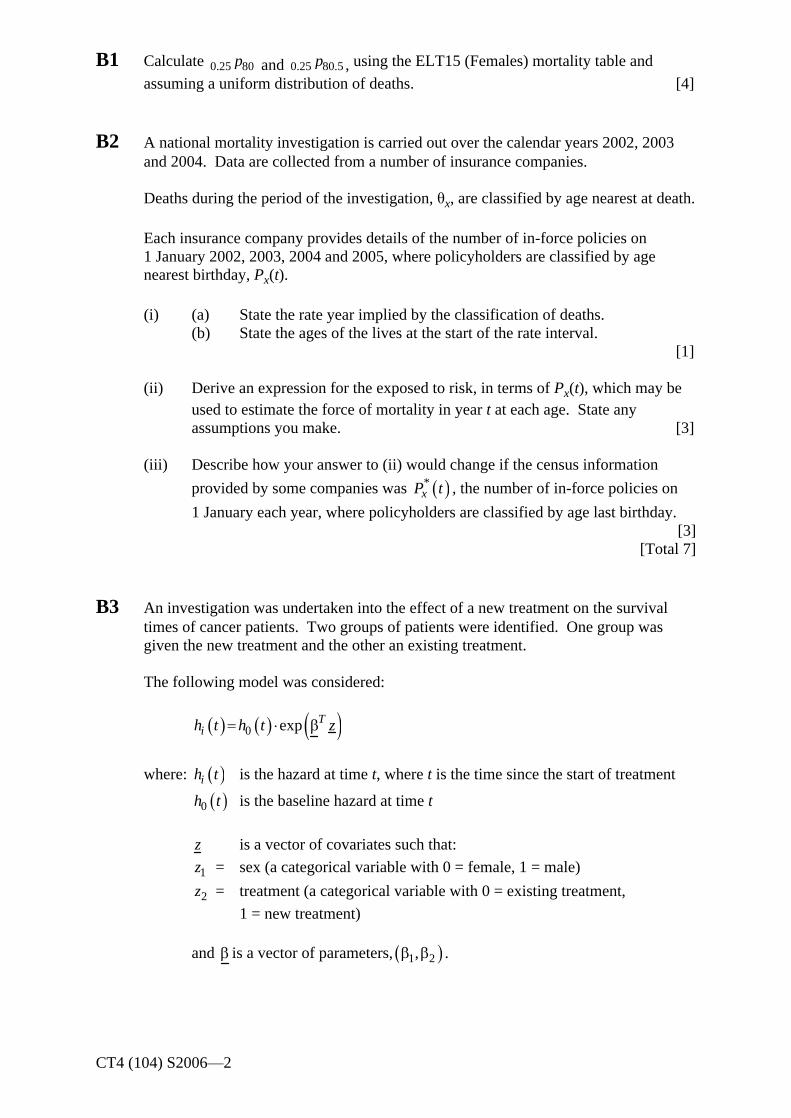
CT4 (104) S2006 2
B1 Calculate 0.25 80p and 0.25 80.5p , using the ELT15 (Females) mortality table and
assuming a uniform distribution of deaths. [4]
B2 A national mortality investigation is carried out over the calendar years 2002, 2003 and 2004. Data are collected from a number of insurance companies.
Deaths during the period of the investigation, x, are classified by age nearest at death.
Each insurance company provides details of the number of in-force policies on 1 January 2002, 2003, 2004 and 2005, where policyholders are classified by age nearest birthday, Px(t).
(i) (a) State the rate year implied by the classification of deaths. (b) State the ages of the lives at the start of the rate interval.
[1]
(ii) Derive an expression for the exposed to risk, in terms of Px(t), which may be used to estimate the force of mortality in year t at each age. State any assumptions you make. [3]
(iii) Describe how your answer to (ii) would change if the census information
provided by some companies was *xP t , the number of in-force policies on
1 January each year, where policyholders are classified by age last birthday. [3]
[Total 7]
B3 An investigation was undertaken into the effect of a new treatment on the survival times of cancer patients. Two groups of patients were identified. One group was given the new treatment and the other an existing treatment.
The following model was considered:
0 exp Tih t h t z
where: ih t
is the hazard at time t, where t is the time since the start of treatment
0h t
is the baseline hazard at time t
z
is a vector of covariates such that:
1z
= sex (a categorical variable with 0 = female, 1 = male)
2z
= treatment (a categorical variable with 0 = existing treatment,
1 = new treatment)
and is a vector of parameters, 1 2, .
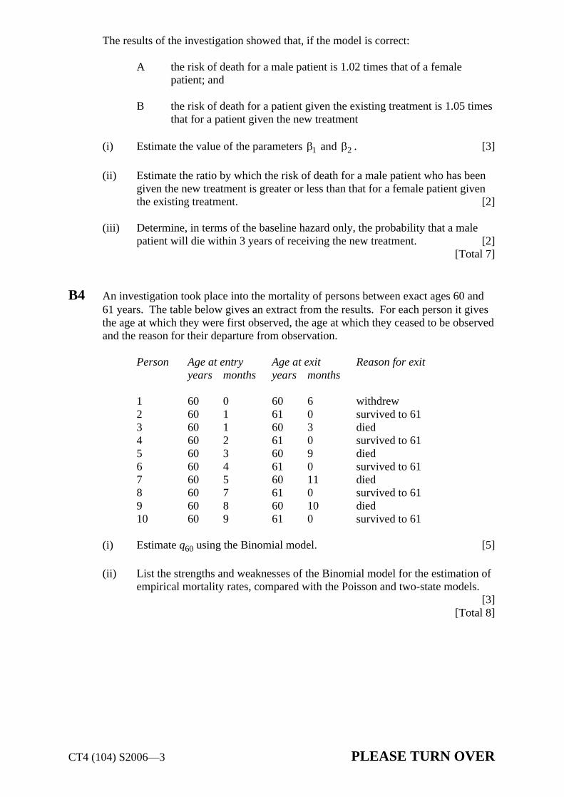
CT4 (104) S2006 3 PLEASE TURN OVER
The results of the investigation showed that, if the model is correct:
A the risk of death for a male patient is 1.02 times that of a female patient; and
B the risk of death for a patient given the existing treatment is 1.05 times that for a patient given the new treatment
(i) Estimate the value of the parameters 1 and 2 . [3]
(ii) Estimate the ratio by which the risk of death for a male patient who has been given the new treatment is greater or less than that for a female patient given the existing treatment. [2]
(iii) Determine, in terms of the baseline hazard only, the probability that a male patient will die within 3 years of receiving the new treatment. [2]
[Total 7]
B4 An investigation took place into the mortality of persons between exact ages 60 and 61 years. The table below gives an extract from the results. For each person it gives the age at which they were first observed, the age at which they ceased to be observed and the reason for their departure from observation.
Person Age at entry Age at exit Reason for exit years months years months
1 60 0 60 6 withdrew 2 60 1 61 0 survived to 61 3 60 1 60 3 died 4 60 2 61 0 survived to 61 5 60 3 60 9 died 6 60 4 61 0 survived to 61 7 60 5 60 11 died 8 60 7 61 0 survived to 61 9 60 8 60 10 died 10 60 9 61 0 survived to 61
(i) Estimate q60 using the Binomial model. [5]
(ii) List the strengths and weaknesses of the Binomial model for the estimation of empirical mortality rates, compared with the Poisson and two-state models.
[3] [Total 8]

CT4 (104) S2006 4
B5 A life insurance company has carried out a mortality investigation. It followed a sample of independent policyholders aged between 50 and 55 years. Policyholders were followed from their 50th birthday until they died, they withdrew from the investigation while still alive, or they celebrated their 55th birthday (whichever of these events occurred first).
(i) Describe the censoring that is present in this investigation. [2]
An extract from the data for 12 policyholders is shown in the table below.
Policyholder Last age at which Outcome policyholder was observed (years and months)
1 50 years 3 months Died 2 50 years 6 months Withdrew
3 51 years 0 months Died 4 51 years 0 months Withdrew
5 52 years 3 months Withdrew
6 52 years 9 months Died 7 53 years 0 months Withdrew
8 53 years 6 months Withdrew
9 54 years 3 months Withdrew
10 54 years 3 months Died 11 55 years 0 months Still alive 12 55 years 0 months Still alive
(ii) Calculate the Nelson-Aalen estimate of the survival function. [5]
(iii) Sketch on a suitably labelled graph the Nelson-Aalen estimate of the survival function. [2]
[Total 9]
B6 (i) (a) Describe the general form of the polynomial formula used to graduate the most recent standard tables produced for use by UK life insurance companies.
(b) Show how the Gompertz and Makeham formulae arise as special cases of this formula.
[3]
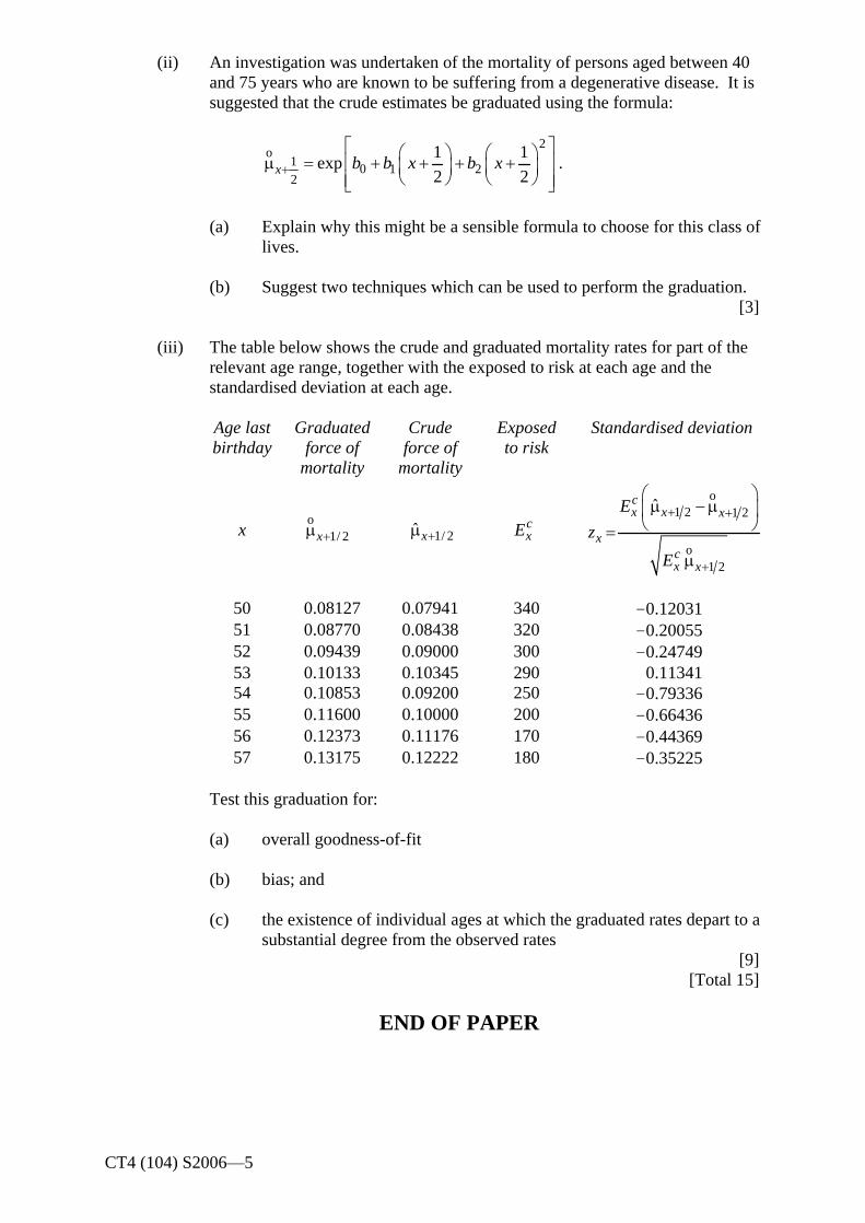
CT4 (104) S2006 5
(ii) An investigation was undertaken of the mortality of persons aged between 40 and 75 years who are known to be suffering from a degenerative disease. It is suggested that the crude estimates be graduated using the formula:
2o
10 1 2
2
1 1exp
2 2x b b x b x .
(a) Explain why this might be a sensible formula to choose for this class of lives.
(b) Suggest two techniques which can be used to perform the graduation. [3]
(iii) The table below shows the crude and graduated mortality rates for part of the relevant age range, together with the exposed to risk at each age and the standardised deviation at each age.
Age last birthday
Graduated force of
mortality
Crude force of
mortality
Exposed to risk
Standardised deviation
x o
1/ 2x
1/ 2x
cxE
o1 2 1 2
o1 2
cx x x
xcx x
E
z
E
50 0.08127 0.07941 340 -0.12031 51 0.08770 0.08438 320 -0.20055 52 0.09439 0.09000 300 -0.24749 53 0.10133 0.10345 290 0.11341 54 0.10853 0.09200 250 -0.79336 55 0.11600 0.10000 200 -0.66436 56 0.12373 0.11176 170 -0.44369 57 0.13175 0.12222 180 -0.35225
Test this graduation for:
(a) overall goodness-of-fit
(b) bias; and
(c) the existence of individual ages at which the graduated rates depart to a substantial degree from the observed rates
[9] [Total 15]
END OF PAPER

Faculty of Actuaries Institute of Actuaries
EXAMINATION
September 2006
Subject CT4 — Models (includes both 103 and 104 parts) Core Technical
EXAMINERS’ REPORT
Introduction The attached subject report has been written by the Principal Examiner with the aim of helping candidates. The questions and comments are based around Core Reading as the interpretation of the syllabus to which the examiners are working. They have however given credit for any alternative approach or interpretation which they consider to be reasonable. M A Stocker Chairman of the Board of Examiners November 2006
© Faculty of Actuaries © Institute of Actuaries

Subject CT4 — Models Core Technical — September 2006 — Examiners’ Report
Page 2
Comments Comments on solutions presented to individual questions for this September 2006 paper are given below. 103 Part Question A1 This was reasonably well answered, even by the weaker candidates.
In part (ii), very few candidates used the information in the question and
calculated 1( )
n
i ii
t s=
−∑ .
Question A2 This was reasonably well answered.
In part (iv), many candidates wrote down a suitable estimate, but failed to provide an explanation as required.
Question A3 This was reasonably well answered.
In part (i), many candidates attempted to describe the simple random walk rather than the general case. In part (ii), very few candidates identified the correct state space for the compound Poisson process or general random walk. In part (iii), credit was not given if the examples cited were not likely to be encountered by an actuary working in a professional capacity.
Question A4 This was not well answered overall, but many of the stronger candidates did
score highly. In part (i), some candidates incorrectly attempted to calculate the long-run probability of being in state B. Part (ii) was generally well answered. In part (iv), the stronger candidates provided good answers, but overall candidates did not score well here.
Question A5 Overall this was poorly answered, although the stronger candidates did well.
Many candidates failed to split the two states labelled B and C in the solution, giving instead a 3-state chain. Some marks were still awarded for the long-run probability calculations in part (iv), but such candidates were not able to calculate the required final answer.
Question A6 This was poorly answered by most candidates, even though some parts of the
question had been asked in previous (103) exams. Marks were lost in all parts of the question. Many candidates did not make a serious attempt at part (iii)(c).

Subject CT4 — Models Core Technical — September 2006 — Examiners’ Report
Page 3
104 Part Question B1 This was well answered.
Some candidates assumed a constant force of mortality, for which credit was not given. Some candidates struggled with the second calculation.
Question B2 This was poorly answered overall, although some of the stronger candidates
did manage to score highly. In part (ii), the question asked candidates to “derive an expression” and therefore we were looking for clearly set out steps here. Many candidates lost marks by not providing sufficient explanation of their working.
Question B3 This was well answered overall.
In parts (i) and (ii), candidates were asked to “estimate” and some indication was required of how the numerical estimate was reached.
Question B4 This was not well answered overall.
In part (i), many candidates did not calculate the correct exposed to risk. Marks were frequently lost because of insufficient working combined with an incorrect final answer. Candidates who wrote down the formulae they were using were given credit even if arithmetic slips were made.
Question B5 This was very well answered by most candidates.
The most common errors were: inconsistency in the assumed order of death and censoring at ages 51 and 54 3/12; and continuation of the estimated survival function after age 55.
Question B6 This was reasonably well answered overall.
Parts (i) and (ii) were poorly answered. In part (iii), the main areas where candidates lost marks were: not correctly stating the null hypothesis; failure to identify the correct degrees of freedom to be used in the chi-squared test; and a failure to state relevant and clear conclusions to the tests.
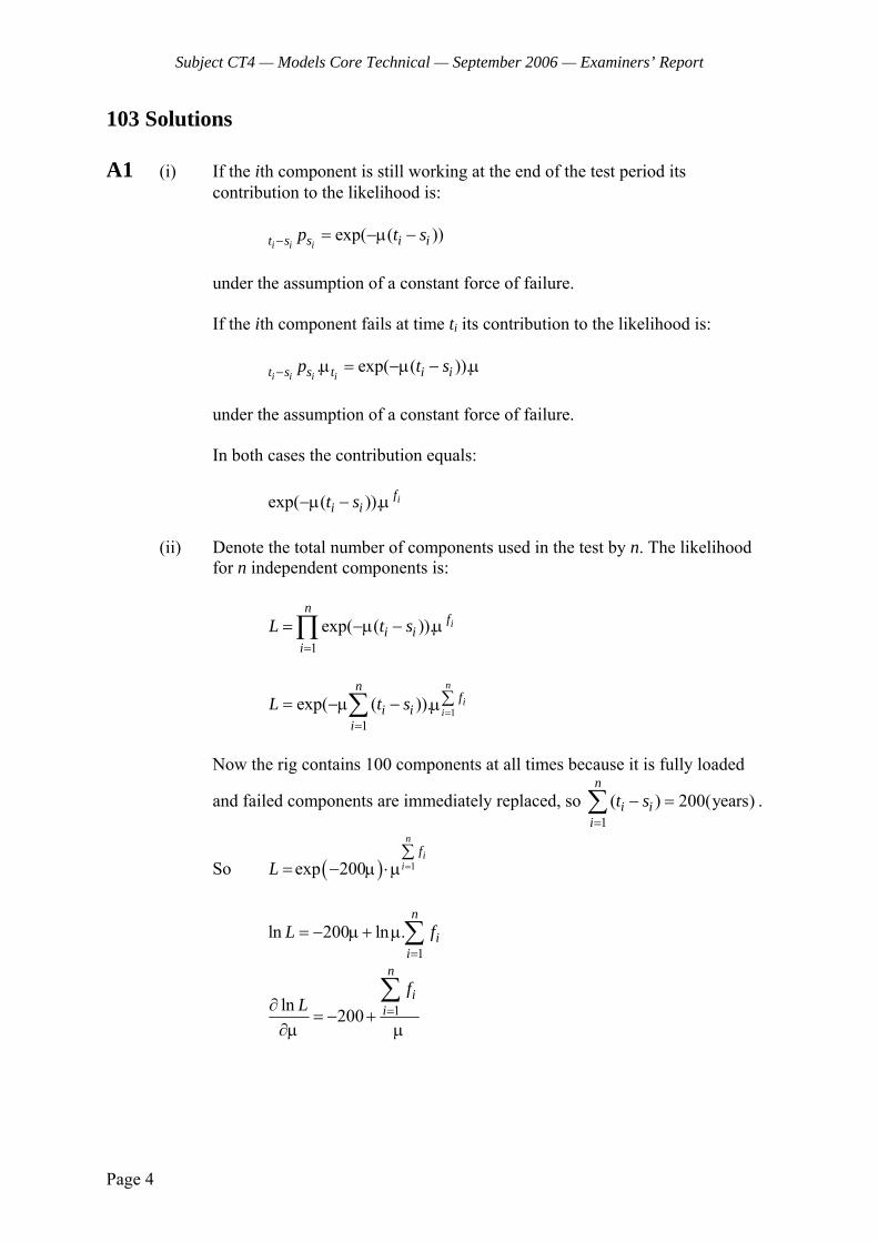
Subject CT4 — Models Core Technical — September 2006 — Examiners’ Report
Page 4
103 Solutions A1 (i) If the ith component is still working at the end of the test period its
contribution to the likelihood is: exp( ( ))
i i it s s i ip t s− = −μ −
under the assumption of a constant force of failure. If the ith component fails at time ti its contribution to the likelihood is: . exp( ( )).
i i i it s s t i ip t s− μ = −μ − μ
under the assumption of a constant force of failure. In both cases the contribution equals: exp( ( )). if
i it s−μ − μ (ii) Denote the total number of components used in the test by n. The likelihood
for n independent components is:
1
exp( ( )). in
fi i
iL t s
=
= −μ − μ∏
11
exp( ( )).n
ii
nf
i ii
L t s=
=
∑= −μ − μ∑
Now the rig contains 100 components at all times because it is fully loaded
and failed components are immediately replaced, so 1
( ) 200(years)n
i ii
t s=
− =∑ .
So ( ) 1exp 200
ni
if
L =∑
= − μ ⋅μ
1
ln 200 ln .n
ii
L f=
= − μ + μ∑
1ln 200
n
ii
fL =∂= − +
∂μ μ
∑
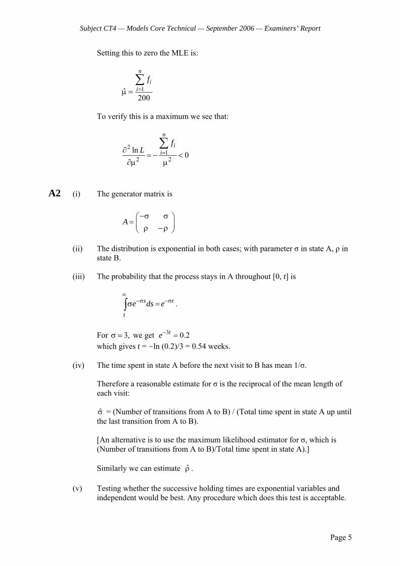
Subject CT4 — Models Core Technical — September 2006 — Examiners’ Report
Page 5
Setting this to zero the MLE is:
1ˆ200
n
ii
f=μ =∑
To verify this is a maximum we see that:
2
12 2
ln 0
n
ii
fL =∂= − <
∂μ μ
∑
A2 (i) The generator matrix is A
−σ σ⎛ ⎞= ⎜ ⎟ρ −ρ⎝ ⎠
(ii) The distribution is exponential in both cases; with parameter σ in state A, ρ in
state B. (iii) The probability that the process stays in A throughout [0, t] is
s t
t
e ds e∞
−σ −σσ =∫ .
For 3,σ = we get 3 0.2te− = which gives t = -ln (0.2)/3 = 0.54 weeks. (iv) The time spent in state A before the next visit to B has mean 1/σ. Therefore a reasonable estimate for σ is the reciprocal of the mean length of
each visit: σ = (Number of transitions from A to B) / (Total time spent in state A up until
the last transition from A to B). [An alternative is to use the maximum likelihood estimator for σ, which is
(Number of transitions from A to B)/Total time spent in state A).] Similarly we can estimate ρ . (v) Testing whether the successive holding times are exponential variables and
independent would be best. Any procedure which does this test is acceptable.
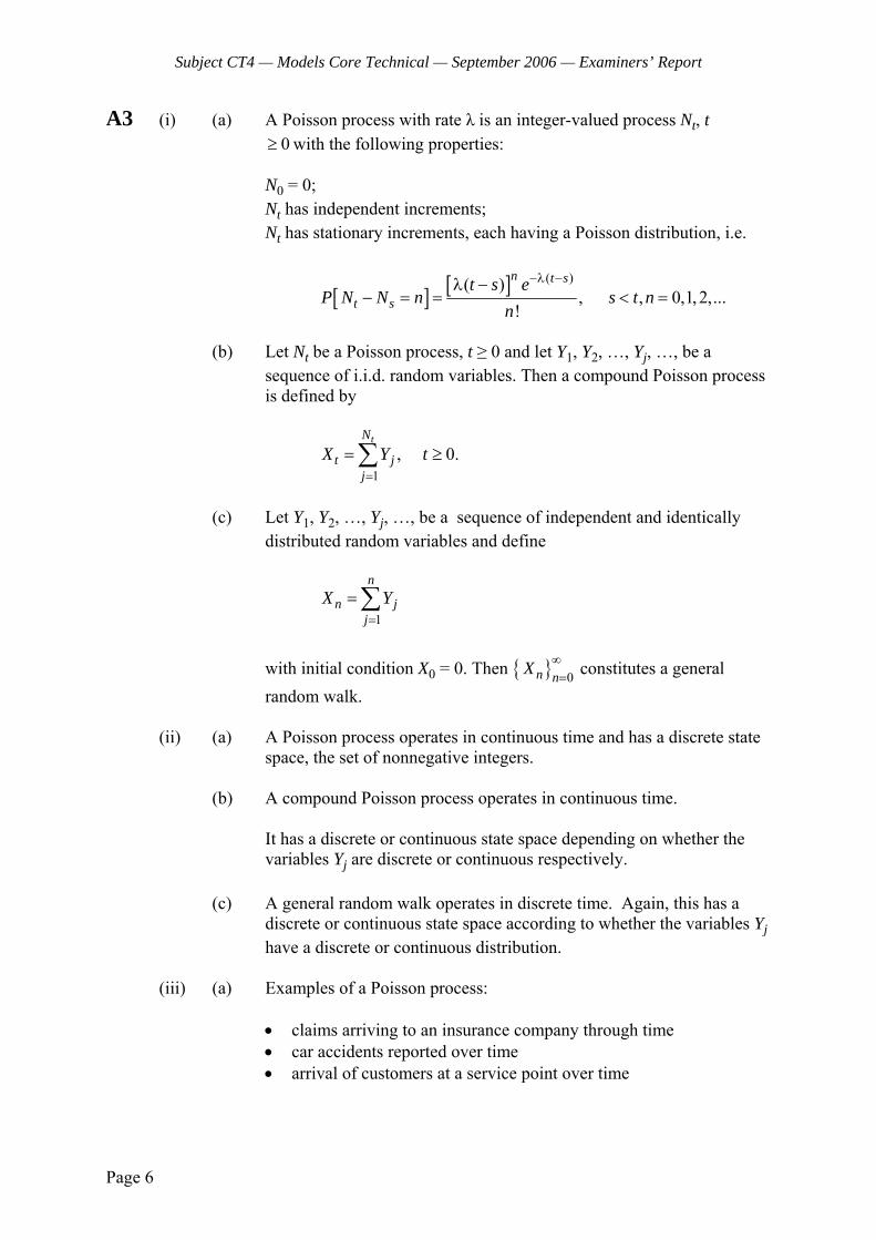
Subject CT4 — Models Core Technical — September 2006 — Examiners’ Report
Page 6
A3 (i) (a) A Poisson process with rate λ is an integer-valued process Nt, t 0≥ with the following properties:
N0 = 0; Nt has independent increments; Nt has stationary increments, each having a Poisson distribution, i.e.
[ ] [ ] ( )( ), , 0,1, 2,...
!
n t s
t st s e
P N N n s t nn
−λ −λ −− = = < =
(b) Let Nt be a Poisson process, t ≥ 0 and let Y1, Y2, …, Yj, …, be a
sequence of i.i.d. random variables. Then a compound Poisson process is defined by
1
, 0.tN
t jj
X Y t=
= ≥∑
(c) Let Y1, Y2, …, Yj, …, be a sequence of independent and identically
distributed random variables and define
1
n
n jj
X Y=
=∑
with initial condition X0 = 0. Then { } 0n nX ∞
= constitutes a general random walk.
(ii) (a) A Poisson process operates in continuous time and has a discrete state
space, the set of nonnegative integers. (b) A compound Poisson process operates in continuous time.
It has a discrete or continuous state space depending on whether the variables Yj are discrete or continuous respectively.
(c) A general random walk operates in discrete time. Again, this has a
discrete or continuous state space according to whether the variables Yj have a discrete or continuous distribution.
(iii) (a) Examples of a Poisson process:
• claims arriving to an insurance company through time • car accidents reported over time • arrival of customers at a service point over time
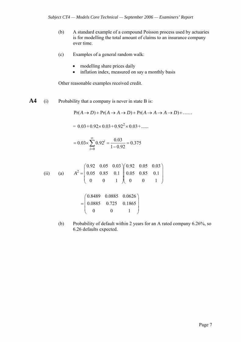
Subject CT4 — Models Core Technical — September 2006 — Examiners’ Report
Page 7
(b) A standard example of a compound Poisson process used by actuaries is for modelling the total amount of claims to an insurance company over time.
(c) Examples of a general random walk:
• modelling share prices daily • inflation index, measured on say a monthly basis
Other reasonable examples received credit. A4 (i) Probability that a company is never in state B is: Pr( ) Pr( ) Pr( )A D A A D A A A D→ + → → + → → → +…… = 20.03+0.92 0.03+ 0.92 0.03+......× ×
0
0.030.03 0.92 0.3751 0.92
i
i
∞
=
= × = =−∑
(ii) (a) 20.92 0.05 0.03 0.92 0.05 0.030.05 0.85 0.1 0.05 0.85 0.1
0 0 1 0 0 1
0.8489 0.0885 0.06260.0885 0.725 0.1865
0 0 1
A⎛ ⎞⎛ ⎞⎜ ⎟⎜ ⎟= ⎜ ⎟⎜ ⎟⎜ ⎟⎜ ⎟⎝ ⎠⎝ ⎠
⎛ ⎞⎜ ⎟= ⎜ ⎟⎜ ⎟⎝ ⎠
(b) Probability of default within 2 years for an A rated company 6.26%, so
6.26 defaults expected.
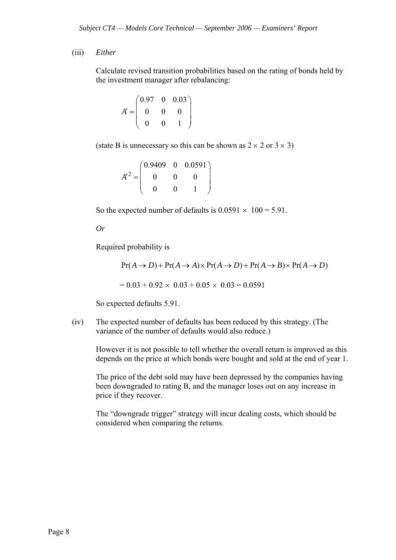
Subject CT4 — Models Core Technical — September 2006 — Examiners’ Report
Page 8
(iii) Either Calculate revised transition probabilities based on the rating of bonds held by
the investment manager after rebalancing:
0.97 0 0.03
0 0 00 0 1
A⎛ ⎞⎜ ⎟′ = ⎜ ⎟⎜ ⎟⎝ ⎠
(state B is unnecessary so this can be shown as 2 × 2 or 3 × 3)
20.9409 0 0.0591
0 0 00 0 1
A⎛ ⎞⎜ ⎟′ = ⎜ ⎟⎜ ⎟⎝ ⎠
So the expected number of defaults is 0.0591 × 100 = 5.91. Or Required probability is Pr( ) Pr( ) Pr( ) Pr( ) Pr( )A D A A A D A B A D→ + → × → + → × → = 0.03 + 0.92 × 0.03 + 0.05 × 0.03 = 0.0591 So expected defaults 5.91. (iv) The expected number of defaults has been reduced by this strategy. (The
variance of the number of defaults would also reduce.) However it is not possible to tell whether the overall return is improved as this
depends on the price at which bonds were bought and sold at the end of year 1. The price of the debt sold may have been depressed by the companies having
been downgraded to rating B, and the manager loses out on any increase in price if they recover.
The “downgrade trigger” strategy will incur dealing costs, which should be
considered when comparing the returns.

Subject CT4 — Models Core Technical — September 2006 — Examiners’ Report
Page 9
A5 (i) Consider the following four states that the policyholder might be at the end of a year:
• the policyholder has made at least one claim both in the year just ended
and the previous one (state A) • the policyholder has made no claims in the year just ended but s/he made
at least one claim during the previous year (state B)
• the policyholder has made at least one claim in the year just ended but not in the previous one (state C)
• the policyholder has made no claim during either the year ended or the
previous one (state D) If the year ended is year n, and Xn denotes the current state of the policyholder,
then Xn constitutes a Markov chain. (ii) The transition matrix is
0.25 0.75 0 00 0 0.15 0.850.15 0.85 0 00 0 0.10 0.90
P
⎛ ⎞⎜ ⎟⎜ ⎟=⎜ ⎟⎜ ⎟⎝ ⎠
(iii) The chain has a finite number of states (A,B,C,D). In order to show that it has
a stationary distribution, it suffices to show that it is irreducible and aperiodic. It is apparent from the transition matrix above that any state can be reached
from any other; hence the chain is irreducible. The chain is also aperiodic since for states A, D the state can remain at the
same state after one step, while for states B, C the state may return to its current state after 2 or 3 steps.
Hence the chain has a stationary distribution (which is unique).
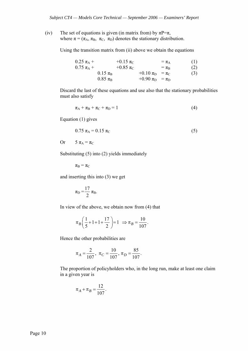
Subject CT4 — Models Core Technical — September 2006 — Examiners’ Report
Page 10
(iv) The set of equations is given (in matrix from) by πP=π, where π = (πA, πB, πC, πD) denotes the stationary distribution. Using the transition matrix from (ii) above we obtain the equations 0.25 πA + +0.15 πC = πA (1) 0.75 πA + +0.85 πC = πB (2) 0.15 πB +0.10 πD = πC (3) 0.85 πB +0.90 πD = πD Discard the last of these equations and use also that the stationary probabilities
must also satisfy πA + πB + πC + πD = 1 (4) Equation (1) gives 0.75 πA = 0.15 πC (5) Or 5 πA = πC Substituting (5) into (2) yields immediately πB = πC and inserting this into (3) we get
πD = 172πB.
In view of the above, we obtain now from (4) that
1 17 101 1 1 .5 2 107B B
⎛ ⎞π + + + = ⇒ π =⎜ ⎟⎝ ⎠
Hence the other probabilities are
2 10 85, , .107 107 107A C Dπ = π = π =
The proportion of policyholders who, in the long run, make at least one claim
in a given year is
12 .107A Bπ + π =
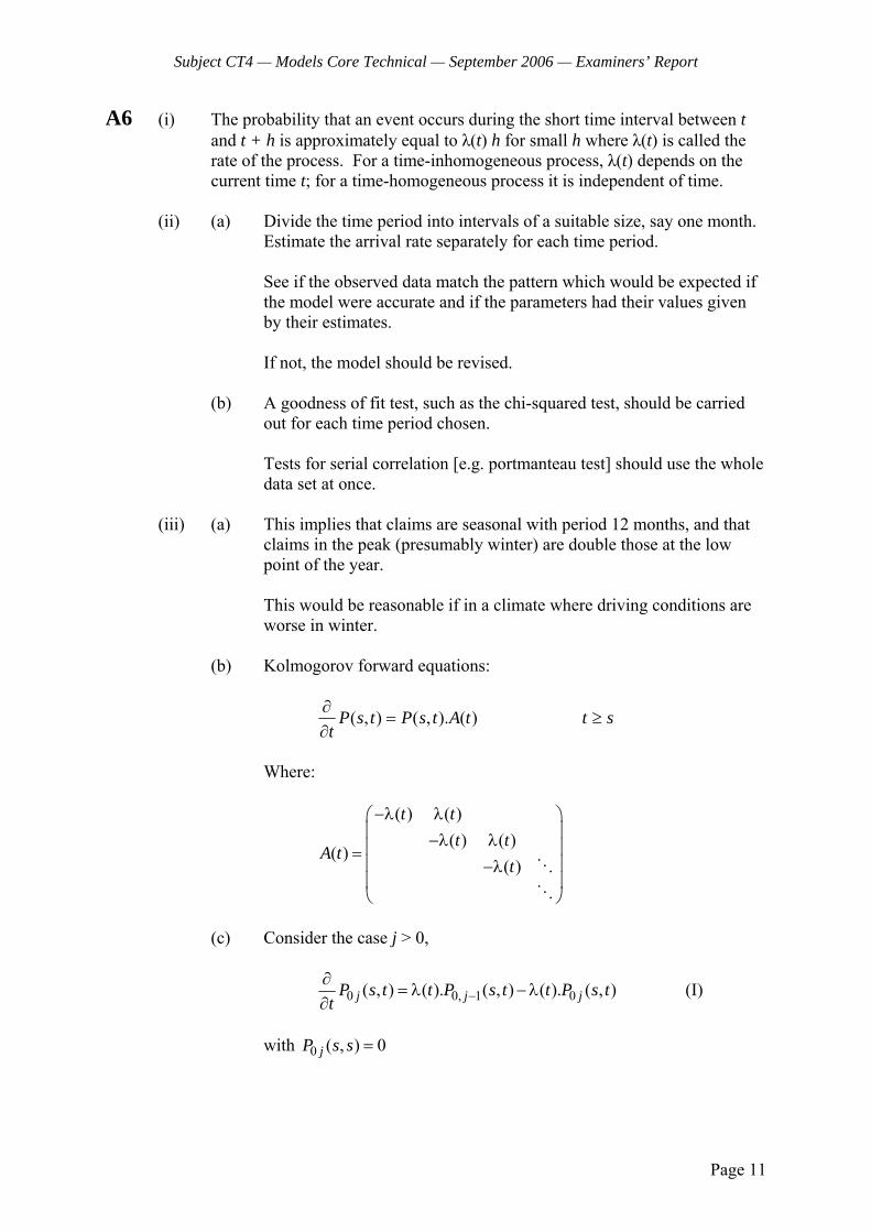
Subject CT4 — Models Core Technical — September 2006 — Examiners’ Report
Page 11
A6 (i) The probability that an event occurs during the short time interval between t and t + h is approximately equal to λ(t) h for small h where λ(t) is called the rate of the process. For a time-inhomogeneous process, λ(t) depends on the current time t; for a time-homogeneous process it is independent of time.
(ii) (a) Divide the time period into intervals of a suitable size, say one month.
Estimate the arrival rate separately for each time period.
See if the observed data match the pattern which would be expected if the model were accurate and if the parameters had their values given by their estimates.
If not, the model should be revised.
(b) A goodness of fit test, such as the chi-squared test, should be carried
out for each time period chosen. Tests for serial correlation [e.g. portmanteau test] should use the whole
data set at once. (iii) (a) This implies that claims are seasonal with period 12 months, and that
claims in the peak (presumably winter) are double those at the low point of the year.
This would be reasonable if in a climate where driving conditions are worse in winter.
(b) Kolmogorov forward equations:
)().,(),( tAtsPtsPt
=∂∂ st ≥
Where:
( ) ( )( ) ( )
( )( )
t tt t
A tt
−λ λ⎛ ⎞⎜ ⎟−λ λ⎜ ⎟=⎜ ⎟−λ⎜ ⎟⎝ ⎠
(c) Consider the case j > 0,
0 0, 1 0( , ) ( ). ( , ) ( ). ( , )j j jP s t t P s t t P s tt −∂
= λ −λ∂
(I)
with 0 ( , ) 0jP s s =
Subject CT4 — Models Core Technical — September 2006 — Examiners’ Report
Page 12
If solution is of the form
0( ( , )) .exp( ( , ))( , )
!
j
jf s t f s tP s t
j−
=
LHS of I
),(.!
)),(exp().),()),(.(( 1 tsfdtd
jtsftsftsfj jj −
−−
RHS of I
1( , ) ( , ) .exp( ( , ))( ). .exp( ( , )) ( ).
( 1)! !
j jf s t f s t f s tt f s t tj j
− −λ − −λ
−
These are equal if
( , ) ( )f s t tt∂
= λ∂
Now
[ ]
( ) (3 cos(2 ))
13 sin(2 )2
13( ) sin(2 ) sin(2 ) ( , )2
t t
s s
t
s
v dv v dv
v v
t s t s f s t
λ = + π
⎡ ⎤= + π⎢ ⎥π⎣ ⎦
= − + π − π ≡π
∫ ∫
this satisfies the boundary condition. Consider the case j = 0
00 00( , ) ( ). ( , )P s t t P s tt∂
= −λ∂
(II)
with boundary condition 00( , ) 1P s s = Need to verify that 00 ( , ) exp( ( , ))P s t f s t= − satisfies II
Subject CT4 — Models Core Technical — September 2006 — Examiners’ Report
Page 13
LHS of II
00exp( ( , )). ( ( , )) ( , ). ( )f s t f s t P s t tt∂
− − = − λ∂
and 00( , ) 1P s s = (d) Solution is of the same form, except that for the homogeneous case
f(s,t) = λ(t-s).
Subject CT4 — Models Core Technical — September 2006 — Examiners’ Report
Page 14
104 Solutions B1 0.25 80 0.25 801p q= − 801 0.25 q= − × under the assumption of a uniform distribution of deaths (UDD) between ages 80 and 81. From ELT 15, q80 = 0.05961, so 0.25 80 1 0.25 0.05961p = − × = 0.98510 ALTERNATIVE 1 Under UDD we have, for 0 s < t 1,
( )1
xt s x s
x
t s qqsq− +
−=
−.
Putting t = 0.75, s = 0.5 and x = 80, therefore,
800.75 0.5 80 0.5
80
0.251 0.5
qqq− + =
−, and so
800.25 80.5
80
0.2511 0.5
qpq
= −−
.
Using ELT15, this is evaluated as
( )( )
0.25 0.05961 0.014901 1 1 0.01536 0.984641 0.5 0.05961 0.97020
− = − = − =−
ALTERNATIVE 2 Using t xp = ,s x t s x sp p− +⋅ 0.75 80p = 0.5 80 0.25 80.5p p⋅ Using an assumption of UDD between ages 80 and 81, we have 0.5 80p = 1 – 0.5 × 0.05961 = 0.97020 0.75 80p = 1 – 0.75 × 0.05961 = 0.95529
Subject CT4 — Models Core Technical — September 2006 — Examiners’ Report
Page 15
So, 0.25 80.5p = 0.75 80
0.5 80
0.95529 0.984630.97020
pp
= =
B2 (i) (a) The age definition changes 6 months before/after each birthday, so this
is a life year rate interval. (b) Lives are aged x - ½ at the start of the rate interval. (ii) Under the principle of correspondence the age definition of deaths and census
should correspond, which they do here. So we do not need to adjust the census information.
The exposed to risk is given by ( )3
0
cx xE P t dt= ∫ .
Assuming Px(t) is linear over calendar years, we can approximate this to
( ) ( )( )2
0
1 12
cx x xE P t P t= + +∑ , where t is measured from 1 January 2002
( ) ( ) ( ) ( )1 10 1 2 32 2x x x xP P P P⎛ ⎞= + + +⎜ ⎟
⎝ ⎠
(iii) The age definitions for deaths and census no longer correspond. So, we need
to adjust the census information for those companies who supply details of ( )*
xP t . Assuming birthdays are uniformly distributed over the calendar year,
we can approximate ( ) ( ) ( )( )* *1
12x x xP t P t P t−≈ + .
And the exposed to risk is then:
( ) ( )( )2
0
1 12
cx x xE P t P t= + +∑
( ) ( )( ) ( ) ( )( )2
* * * *1 1
0
1 1 1 1 12 2 2x x x xP t P t P t P t− −⎛ ⎞= + + + + +⎜ ⎟⎝ ⎠
∑
( ) ( )( ) ( ) ( ) ( ) ( )( ) ( ) ( )( )* * * * * * * *1 1 1 1
1 1 10 0 1 1 2 2 3 34 2 4x x x x x x x xP P P P P P P P− − − −= + + + + + + +
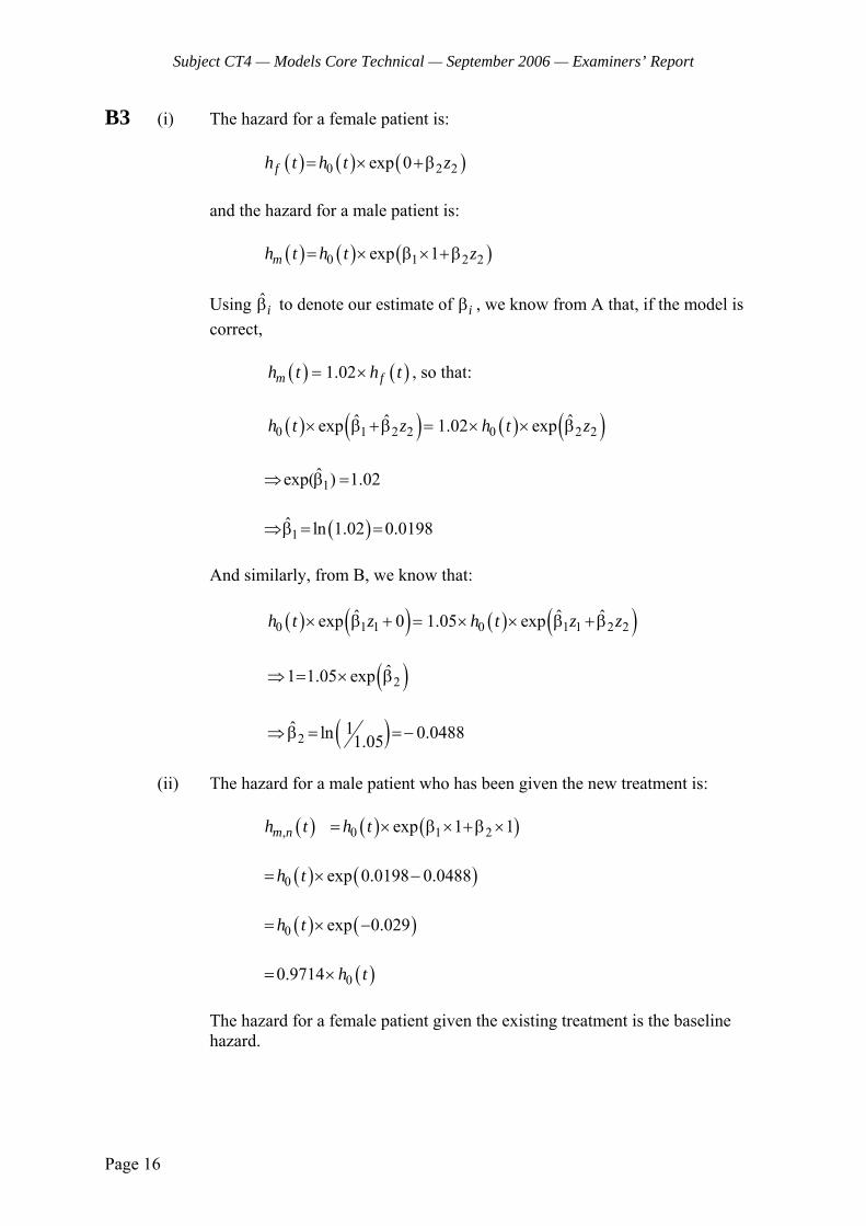
Subject CT4 — Models Core Technical — September 2006 — Examiners’ Report
Page 16
B3 (i) The hazard for a female patient is: ( ) ( ) ( )0 2 2exp 0fh t h t z= × +β and the hazard for a male patient is: ( ) ( ) ( )0 1 2 2exp 1mh t h t z= × β × +β Using ˆ
iβ to denote our estimate of iβ , we know from A that, if the model is correct,
( ) ( )1.02m fh t h t= × , so that: ( ) ( ) ( ) ( )0 1 2 2 0 2 2
ˆ ˆ ˆexp 1.02 exph t z h t z× β +β = × × β
1
ˆexp( ) 1.02⇒ β = ( )1
ˆ ln 1.02 0.0198⇒β = = And similarly, from B, we know that: ( ) ( ) ( ) ( )0 1 1 0 1 1 2 2
ˆ ˆ ˆexp 0 1.05 exph t z h t z z× β + = × × β +β
( )2
ˆ1 1.05 exp⇒ = × β
( )2
ˆ 1ln 0.04881.05⇒β = =−
(ii) The hazard for a male patient who has been given the new treatment is: ( ) ( ) ( ), 0 1 2exp 1 1m nh t h t= × β × +β × ( ) ( )0 exp 0.0198 0.0488h t= × − ( ) ( )0 exp 0.029h t= × − ( )00.9714 h t= × The hazard for a female patient given the existing treatment is the baseline
hazard.
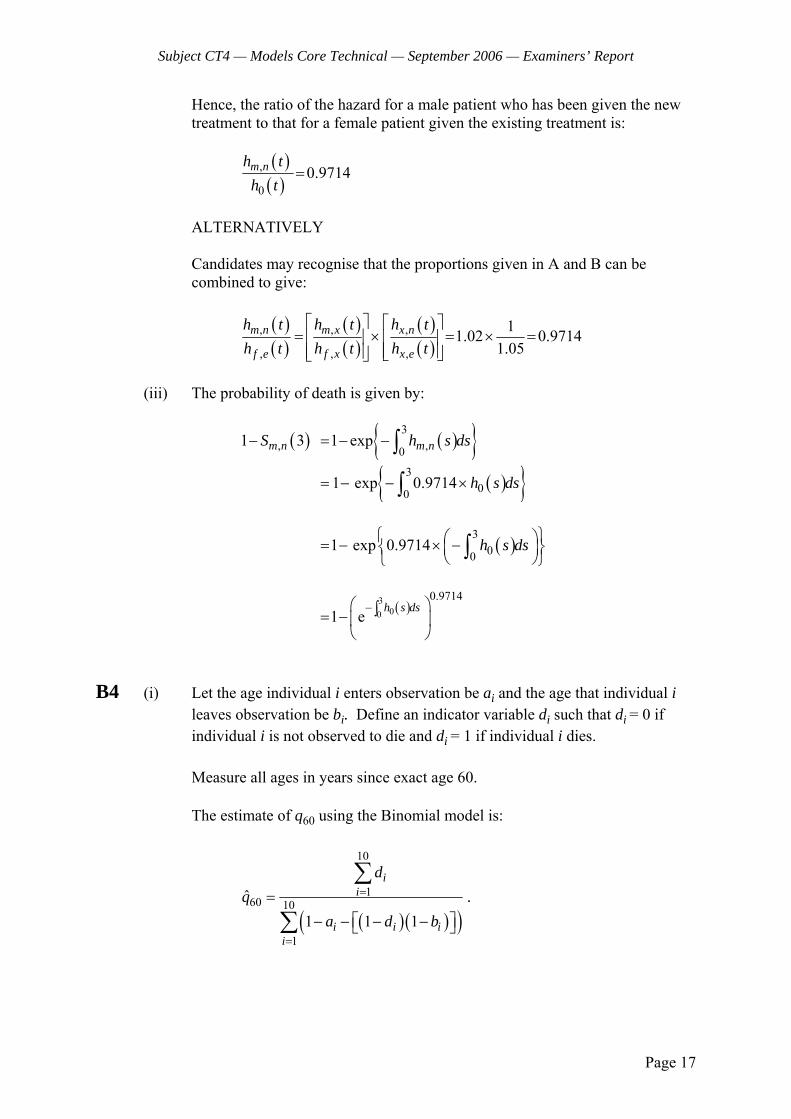
Subject CT4 — Models Core Technical — September 2006 — Examiners’ Report
Page 17
Hence, the ratio of the hazard for a male patient who has been given the new treatment to that for a female patient given the existing treatment is:
( )( )
,
00.9714m nh t
h t=
ALTERNATIVELY Candidates may recognise that the proportions given in A and B can be
combined to give:
( )( )
( )( )
( )( )
, , ,
, , ,
11.02 0.97141.05
m n m x x n
f e f x x e
h t h t h th t h t h t
⎡ ⎤ ⎡ ⎤= × = × =⎢ ⎥ ⎢ ⎥
⎢ ⎥⎢ ⎥ ⎣ ⎦⎣ ⎦
(iii) The probability of death is given by:
( ) ( ){ }3, ,0
1 3 1 expm n m nS h s ds− = − −∫
( ){ }300
1 exp 0.9714 h s ds= − − ×∫
( )3
001 exp 0.9714 h s ds⎧ ⎫⎛ ⎞= − × −⎨ ⎬⎜ ⎟
⎝ ⎠⎩ ⎭∫
( )300
0.9714
1 e h s ds−⎛ ⎞∫= −⎜ ⎟⎝ ⎠
B4 (i) Let the age individual i enters observation be ai and the age that individual i
leaves observation be bi. Define an indicator variable di such that di = 0 if individual i is not observed to die and di = 1 if individual i dies.
Measure all ages in years since exact age 60. The estimate of q60 using the Binomial model is:
( )( )( )
10
160 10
1
ˆ1 1 1
ii
i i ii
dq
a d b
=
=
=⎡ ⎤− − − −⎣ ⎦
∑
∑.
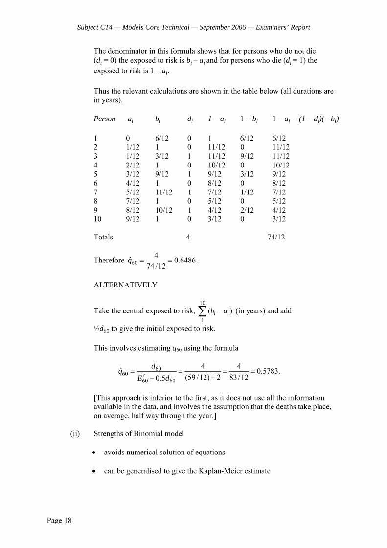
Subject CT4 — Models Core Technical — September 2006 — Examiners’ Report
Page 18
The denominator in this formula shows that for persons who do not die (di = 0) the exposed to risk is bi – ai and for persons who die (di = 1) the exposed to risk is 1 – ai.
Thus the relevant calculations are shown in the table below (all durations are
in years).
Person ai bi di 1 - ai 1 – bi 1 - ai - (1 - di)(- bi) 1 0 6/12 0 1 6/12 6/12 2 1/12 1 0 11/12 0 11/12 3 1/12 3/12 1 11/12 9/12 11/12 4 2/12 1 0 10/12 0 10/12 5 3/12 9/12 1 9/12 3/12 9/12 6 4/12 1 0 8/12 0 8/12 7 5/12 11/12 1 7/12 1/12 7/12 8 7/12 1 0 5/12 0 5/12 9 8/12 10/12 1 4/12 2/12 4/12 10 9/12 1 0 3/12 0 3/12 Totals 4 74/12
Therefore 604ˆ 0.6486
74 /12q = = .
ALTERNATIVELY
Take the central exposed to risk, 10
1( )i ib a−∑ (in years) and add
½d60 to give the initial exposed to risk.
This involves estimating q60 using the formula
6060
60 60
4 4ˆ 0.5783.(59 /12) 2 83/120.5c
dqE d
= = = =++
[This approach is inferior to the first, as it does not use all the information
available in the data, and involves the assumption that the deaths take place, on average, half way through the year.]
(ii) Strengths of Binomial model
• avoids numerical solution of equations • can be generalised to give the Kaplan-Meier estimate
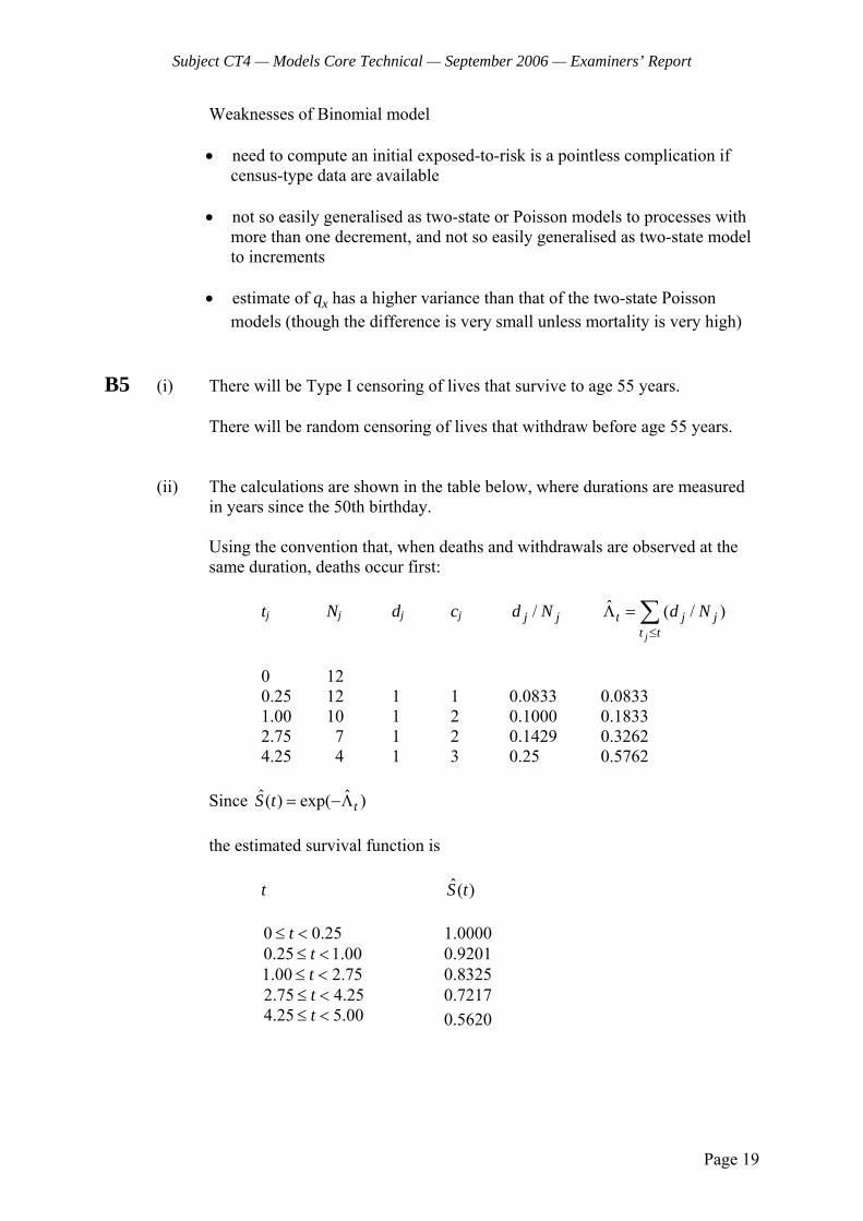
Subject CT4 — Models Core Technical — September 2006 — Examiners’ Report
Page 19
Weaknesses of Binomial model
• need to compute an initial exposed-to-risk is a pointless complication if census-type data are available
• not so easily generalised as two-state or Poisson models to processes with
more than one decrement, and not so easily generalised as two-state model to increments
• estimate of qx has a higher variance than that of the two-state Poisson models (though the difference is very small unless mortality is very high)
B5 (i) There will be Type I censoring of lives that survive to age 55 years. There will be random censoring of lives that withdraw before age 55 years. (ii) The calculations are shown in the table below, where durations are measured
in years since the 50th birthday. Using the convention that, when deaths and withdrawals are observed at the same duration, deaths occur first:
tj Nj dj cj /j jd N ˆ ( / )
j
t j jt t
d N≤
Λ = ∑
0 12 0.25 12 1 1 0.0833 0.0833 1.00 10 1 2 0.1000 0.1833 2.75 7 1 2 0.1429 0.3262 4.25 4 1 3 0.25 0.5762
Since ˆ ˆ( ) exp( )tS t = −Λ the estimated survival function is
t ˆ( )S t 0 0.25t≤ < 1.0000 0.25 1.00t≤ < 0.9201 1.00 2.75t≤ < 0.8325 2.75 4.25t≤ < 0.7217 4.25 5.00t≤ < 0.5620
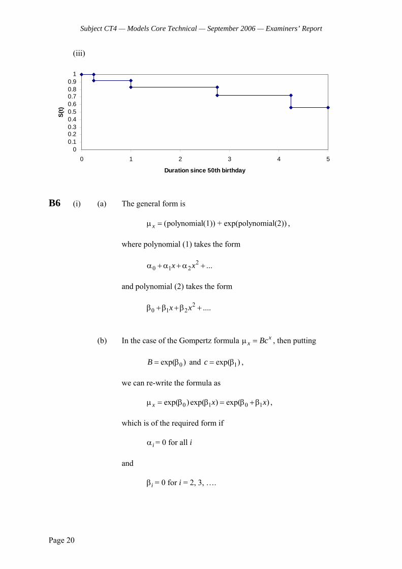
Subject CT4 — Models Core Technical — September 2006 — Examiners’ Report
Page 20
(iii)
B6 (i) (a) The general form is (polynomial(1)) + exp(polynomial(2))xμ = , where polynomial (1) takes the form 2
0 1 2 ...x xα +α +α + and polynomial (2) takes the form 2
0 1 2 ....x xβ +β +β + (b) In the case of the Gompertz formula x
x Bcμ = , then putting 0exp( )B = β and 1exp( )c = β , we can re-write the formula as 0 1 0 1exp( )exp( ) exp( )x x xμ = β β = β +β , which is of the required form if
iα = 0 for all i
and
iβ = 0 for i = 2, 3, ….
00.10.20.30.40.50.60.70.80.9
1
0 0.5 1 1.5 2 2.5 3 3.5 4 4.5 5
Duration since 50th birthday
S(t)
00.10.20.30.40.50.60.70.80.9
1
0 1 2 3 4 5
Duration since 50th birthday
S(t)
Subject CT4 — Models Core Technical — September 2006 — Examiners’ Report
Page 21
Similarly the Makeham formula xx A Bcμ = +
can be expressed in the required form by putting 0A = α , 0exp( )B = β and 1exp( )c = β . (ii) (a) The Gompertz formula written 0 1exp( )x xμ = β +β is an exponential function which implies that the rate of increase of
mortality with age is constant. This is often a reasonable assumption for ordinary lives at middle ages
and older ages. In the special case of the impaired lives known to be suffering from a
degenerative disease, it is plausible to suppose that the rate of increase of mortality might increase with age.
The term 2
212
b x⎛ ⎞+⎜ ⎟⎝ ⎠
in the formula can allow for this possibility.
(b) The graduation can be achieved by maximum likelihood estimation of the parameters or by ordinary least squares regression
of 12
ˆlogx+
⎡ ⎤⎢ ⎥μ⎢ ⎥⎣ ⎦
on 12
x + and 21 .
2x⎛ ⎞+⎜ ⎟
⎝ ⎠
(iii) (a) The null hypothesis is that there is no difference between the graduated
rates and the underlying rates in the population from which the crude rates are derived.
To test overall goodness-of-fit we use the chi-squared test. 2 2
x mx
z χ∑ ∼ ,
where m is the number of degrees of freedom. In this case, we have 8 ages, but 3 parameters were estimated when
performing the graduation, so m = 5.
Subject CT4 — Models Core Technical — September 2006 — Examiners’ Report
Page 22
The calculations are shown in the table below.
Age x zx 2
xz last
birthday 50 -0.12031 0.01447 51 -0.20055 0.04022 52 -0.24749 0.06125 53 0.11341 0.01286 54 -0.79336 0.62942 55 -0.66436 0.44137 56 -0.44369 0.19686 57 -0.35225 0.12408 Sum 1.52053 The critical value of the chi-squared distribution with 5 degrees of
freedom at the 5 per cent level is 11.07. Since 1.52052 11.07, we do not reject the null hypothesis and
conclude that the graduation adheres satisfactorily to the data. (b) To test for bias we use EITHER the Signs Test or the Cumulative
Deviations test. Signs Test The test statistic, P, is the number of signs that is positive. Under the null hypothesis, ~ Binomial(8,0.5)P In this case P = 1, and Prob[ 1P ≤ ] = 0.0352. Since this probability > 0.025 (two-tailed test) we do not reject the null
hypothesis. We conclude that the graduated rates are not biased above or below the
crude rates.
Subject CT4 — Models Core Technical — September 2006 — Examiners’ Report
Page 23
Cumulative deviations test The test statistic
o1122
o12
ˆ( )
~ Normal(0,1)x xxxx
xxx
E E
E
++
+
μ −μ
μ
∑
∑.
The calculations are shown in the table below.
Age x o
1122
ˆ x xxxE E++
μ −μ o
12
xx E+μ
last birthday 50 -0.63 27.63 51 -1.06 28.06 52 -1.32 28.32 53 0.61 29.39 54 -4.13 27.13 55 -3.20 23.20 56 -2.03 21.03 57 -1.72 23.72 Sum -13.48 208.48
The value of the test statistic is therefore (-13.48/√208.48) = -0.9335. using a two-tailed test, the absolute value of the test statistics is less
than 1.96, so we do not reject the null hypothesis. We conclude that the graduated rates are not biased above or below the
crude rates. (c) To test for the existence of individual ages at which the graduated rates
depart greatly from the observed rates we can use the Individual Standardised Deviations Test.
There are no ages at which the absolute value of zx exceeds 1.96. Therefore we do not reject the null hypothesis and conclude that there
are no outliers.
END OF EXAMINERS’ REPORT

Faculty of Actuaries Institute of Actuaries
EXAMINATION
20 April 2007 (am)
Subject CT4 — Models Core Technical
Time allowed: Three hours
INSTRUCTIONS TO THE CANDIDATE
1. Enter all the candidate and examination details as requested on the front of your answer booklet.
2. You must not start writing your answers in the booklet until instructed to do so by the
supervisor. 3. Mark allocations are shown in brackets. 4. Attempt all 11 questions, beginning your answer to each question on a separate sheet. 5. Candidates should show calculations where this is appropriate.
Graph paper is not required for this paper.
AT THE END OF THE EXAMINATION
Hand in BOTH your answer booklet, with any additional sheets firmly attached, and this question paper.
In addition to this paper you should have available the 2002 edition of the Formulae and Tables and your own electronic calculator.
© Faculty of Actuaries CT4 A2007 © Institute of Actuaries
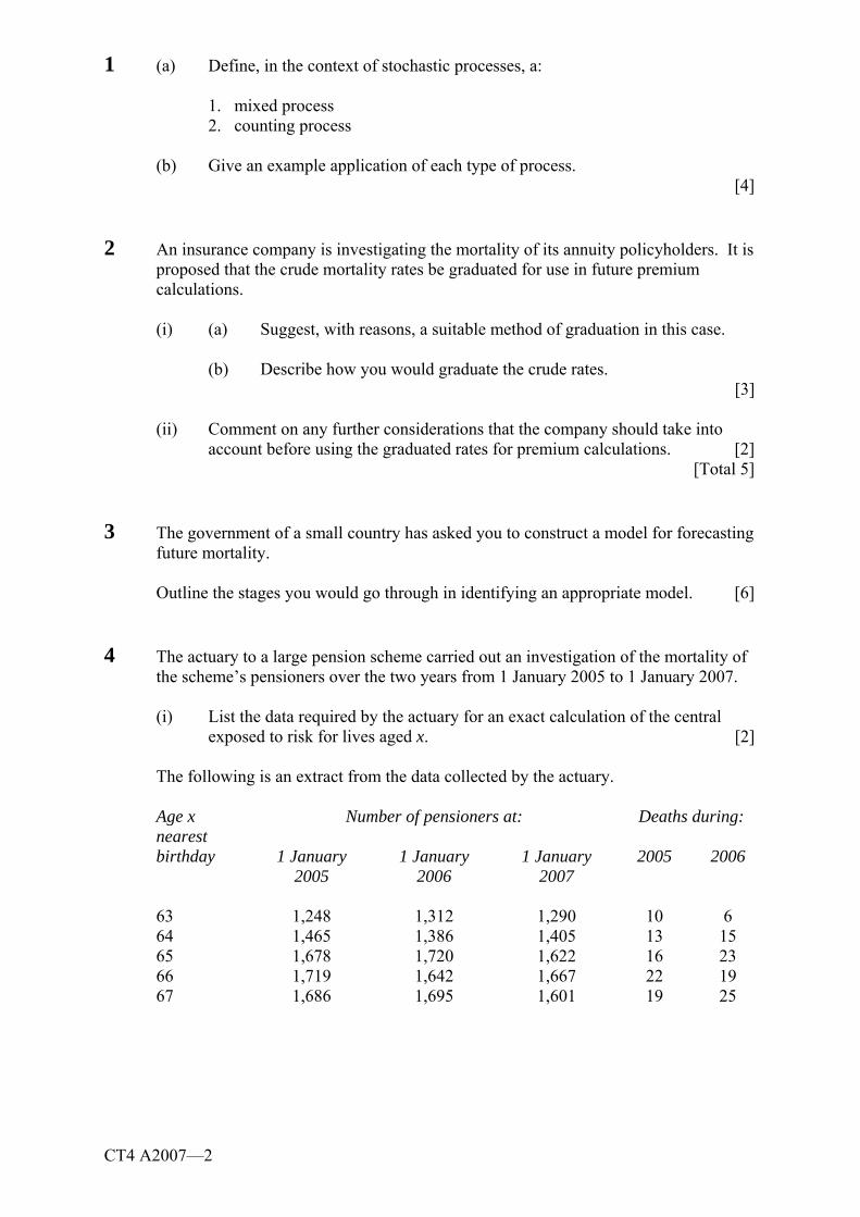
CT4 A2007—2
1 (a) Define, in the context of stochastic processes, a:
1. mixed process 2. counting process
(b) Give an example application of each type of process. [4] 2 An insurance company is investigating the mortality of its annuity policyholders. It is
proposed that the crude mortality rates be graduated for use in future premium calculations. (i) (a) Suggest, with reasons, a suitable method of graduation in this case.
(b) Describe how you would graduate the crude rates. [3]
(ii) Comment on any further considerations that the company should take into account before using the graduated rates for premium calculations. [2]
[Total 5] 3 The government of a small country has asked you to construct a model for forecasting
future mortality. Outline the stages you would go through in identifying an appropriate model. [6]
4 The actuary to a large pension scheme carried out an investigation of the mortality of
the scheme’s pensioners over the two years from 1 January 2005 to 1 January 2007.
(i) List the data required by the actuary for an exact calculation of the central exposed to risk for lives aged x. [2]
The following is an extract from the data collected by the actuary. Age x nearest
Number of pensioners at: Deaths during:
birthday
1 January 2005
1 January 2006
1 January 2007
2005 2006
63 1,248 1,312 1,290 10 6 64 1,465 1,386 1,405 13 15 65 1,678 1,720 1,622 16 23 66 1,719 1,642 1,667 22 19 67 1,686 1,695 1,601 19 25
CT4 A2007—3 PLEASE TURN OVER
(ii) (a) Derive an expression that could be used to estimate the central exposed to risk using the available data. State any assumptions you make.
(b) Use the data to estimate 65μ . State any further assumptions that you
make. [4] [Total 6] 5 (i) Define the hazard rate, h(t), of a random variable T denoting lifetime. [1]
(ii) An investigation is undertaken into the mortality of men aged between exact ages 50 and 55 years. A sample of n men is followed from their 50th birthdays until either they die or they reach their 55th birthdays.
The hazard of death (or force of mortality) between these ages, h(t), is assumed to have the following form:
( )h t t= α +β where α and β are parameters to be estimated and t is measured in years since the 50th birthday. (a) Derive an expression for the survival function between ages 50 and 55
years.
(b) Sketch this on a graph. (c) Comment on the appropriateness of the assumed form of the hazard for
modelling mortality over this age range. [6] [Total 7]
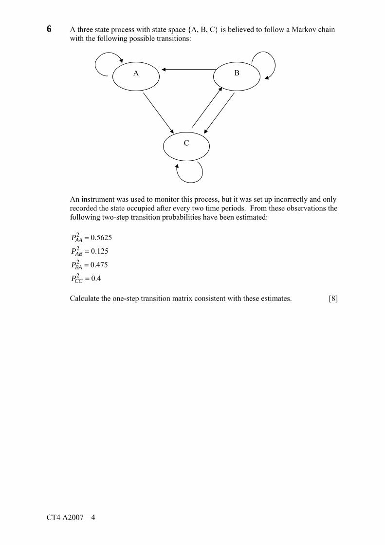
CT4 A2007—4
6 A three state process with state space {A, B, C} is believed to follow a Markov chain with the following possible transitions:
An instrument was used to monitor this process, but it was set up incorrectly and only recorded the state occupied after every two time periods. From these observations the following two-step transition probabilities have been estimated:
2 0.5625AAP = 2 0.125ABP = 2 0.475BAP = 2 0.4CCP =
Calculate the one-step transition matrix consistent with these estimates. [8]
A B
C

CT4 A2007—5 PLEASE TURN OVER
7 Every person has two chromosomes, each being a copy of one of the chromosomes from one of their parents. There are two types of chromosomes labelled X and Y. A child born with an X and a Y chromosome is male and a child with two X chromosomes is female.
The blood-clotting disorder haemophilia is caused by a defective X chromosome (X*). A female with the defective chromosome (X*X) will not usually exhibit symptoms of the disease but may pass the defective gene to her children and so is known as a carrier. A male with the defective chromosome (X*Y) suffers from the disease and is known as a haemophiliac.
A medical researcher wishes to study the progress of the disease through the first born child in each generation, starting with a female carrier.
You may assume: • every parent has a equal chance of passing either of their chromosomes to their
children • the partner of each person in the study does not carry a defective X chromosome;
and • no new genetic defects occur
(i) Show that the expected progress of the disease through the generations may be
modelled as a Markov chain and specify carefully:
(a) the state space; and (b) the transition diagram [5]
(ii) State, with reasons, whether the chain is:
(a) irreducible; and (b) aperiodic [2]
(iii) Calculate the stationary distribution of the Markov chain. [3]
[Total 10]

CT4 A2007—6
8 A medical study was carried out between 1 January 2001 and 1 January 2006, to assess the survival rates of cancer patients. The patients all underwent surgery during 2001 and then attended 3-monthly check-ups throughout the study.
The following data were collected: For those patients who died during the study exact dates of death were recorded as follows: Patient Date of surgery Date of death
A 1 April 2001 1 August 2005 B 1 April 2001 1 October 2001 C 1 May 2001 1 March 2002 D 1 September 2001 1 August 2003 E 1 October 2001 1 August 2002 For those patients who survived to the end of the study: Patient
Date of surgery
F 1 February 2001 G 1 March 2001 H 1 April 2001 I 1 June 2001 J 1 September 2001 K 1 September 2001 L 1 November 2001 For those patients with whom the hospital lost contact before the end of the investigation: Patient
Date of surgery Date of last check-up
M 1 February 2001 1 August 2003 N 1 June 2001 1 March 2002 O 1 September 2001 1 September 2005 (i) Explain whether and where each of the following types of censoring is present
in this investigation: (a) type I censoring (b) interval censoring; and (c) informative censoring [3]
(ii) Calculate the Kaplan-Meier estimate of the survival function for these patients. State any assumptions that you make. [7]
(iii) Hence estimate the probability that a patient will die within 4 years of surgery.
[1] [Total 11]
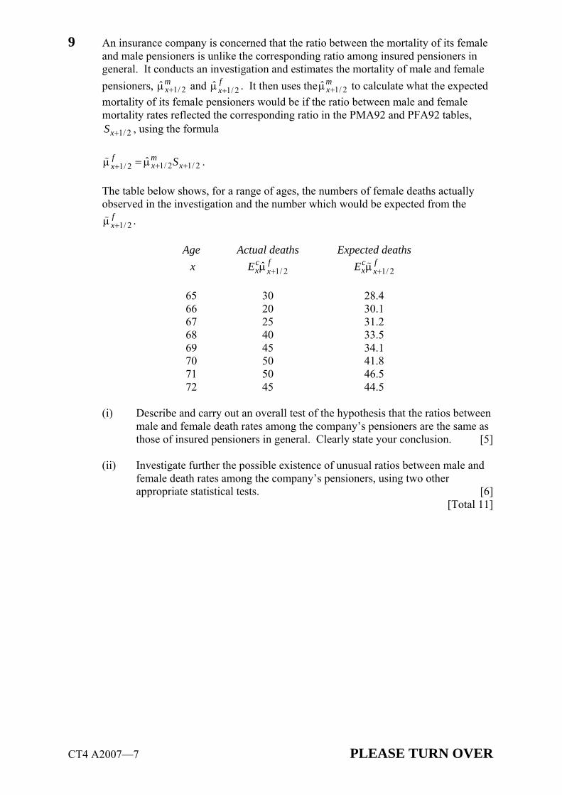
CT4 A2007—7 PLEASE TURN OVER
9 An insurance company is concerned that the ratio between the mortality of its female and male pensioners is unlike the corresponding ratio among insured pensioners in general. It conducts an investigation and estimates the mortality of male and female pensioners, 1/ 2ˆ m
x+μ and 1/ 2ˆ fx+μ . It then uses the 1/ 2ˆ m
x+μ to calculate what the expected mortality of its female pensioners would be if the ratio between male and female mortality rates reflected the corresponding ratio in the PMA92 and PFA92 tables,
1/ 2xS + , using the formula
1/ 2 1/ 21/ 2 ˆf mx xx S+ ++μ = μ .
The table below shows, for a range of ages, the numbers of female deaths actually observed in the investigation and the number which would be expected from the
1/ 2fx+μ .
Age Actual deaths Expected deaths x 1/ 2ˆ fc
x xE +μ 1/ 2fc
x xE +μ 65 30 28.4 66 20 30.1 67 25 31.2 68 40 33.5 69 45 34.1 70 50 41.8 71 50 46.5 72 45 44.5 (i) Describe and carry out an overall test of the hypothesis that the ratios between
male and female death rates among the company’s pensioners are the same as those of insured pensioners in general. Clearly state your conclusion. [5]
(ii) Investigate further the possible existence of unusual ratios between male and
female death rates among the company’s pensioners, using two other appropriate statistical tests. [6]
[Total 11]
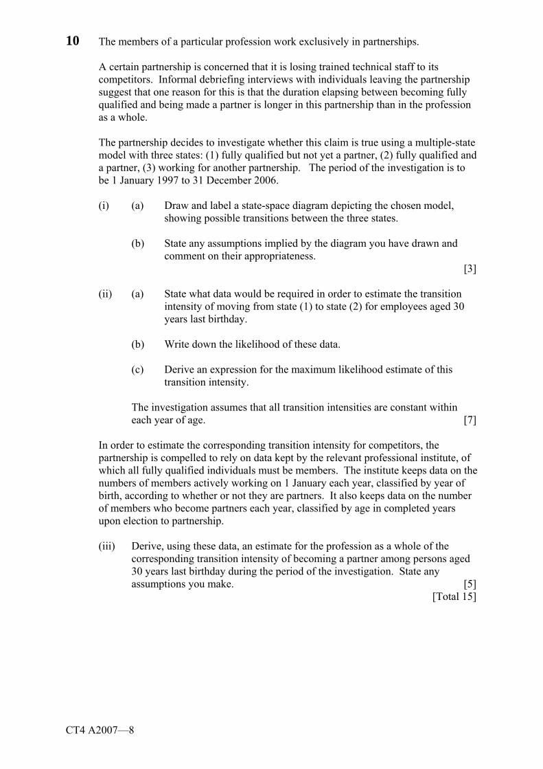
CT4 A2007—8
10 The members of a particular profession work exclusively in partnerships.
A certain partnership is concerned that it is losing trained technical staff to its competitors. Informal debriefing interviews with individuals leaving the partnership suggest that one reason for this is that the duration elapsing between becoming fully qualified and being made a partner is longer in this partnership than in the profession as a whole. The partnership decides to investigate whether this claim is true using a multiple-state model with three states: (1) fully qualified but not yet a partner, (2) fully qualified and a partner, (3) working for another partnership. The period of the investigation is to be 1 January 1997 to 31 December 2006. (i) (a) Draw and label a state-space diagram depicting the chosen model,
showing possible transitions between the three states.
(b) State any assumptions implied by the diagram you have drawn and comment on their appropriateness.
[3] (ii) (a) State what data would be required in order to estimate the transition
intensity of moving from state (1) to state (2) for employees aged 30 years last birthday.
(b) Write down the likelihood of these data.
(c) Derive an expression for the maximum likelihood estimate of this
transition intensity.
The investigation assumes that all transition intensities are constant within each year of age. [7]
In order to estimate the corresponding transition intensity for competitors, the partnership is compelled to rely on data kept by the relevant professional institute, of which all fully qualified individuals must be members. The institute keeps data on the numbers of members actively working on 1 January each year, classified by year of birth, according to whether or not they are partners. It also keeps data on the number of members who become partners each year, classified by age in completed years upon election to partnership. (iii) Derive, using these data, an estimate for the profession as a whole of the
corresponding transition intensity of becoming a partner among persons aged 30 years last birthday during the period of the investigation. State any assumptions you make. [5]
[Total 15]
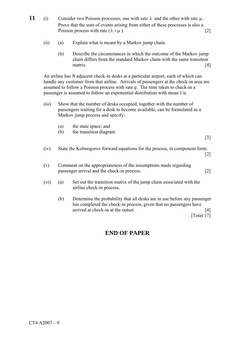
CT4 A2007—9
11 (i) Consider two Poisson processes, one with rate λ and the other with rate μ . Prove that the sum of events arising from either of these processes is also a Poisson process with rate (λ +μ ). [2]
(ii) (a) Explain what is meant by a Markov jump chain.
(b) Describe the circumstances in which the outcome of the Markov jump
chain differs from the standard Markov chain with the same transition matrix. [4]
An airline has N adjacent check-in desks at a particular airport, each of which can handle any customer from that airline. Arrivals of passengers at the check-in area are assumed to follow a Poisson process with rate q. The time taken to check-in a passenger is assumed to follow an exponential distribution with mean 1/a.
(iii) Show that the number of desks occupied, together with the number of
passengers waiting for a desk to become available, can be formulated as a Markov jump process and specify:
(a) the state space; and (b) the transition diagram [3]
(iv) State the Kolmogorov forward equations for the process, in component form. [2]
(v) Comment on the appropriateness of the assumptions made regarding
passenger arrival and the check-in process. [2]
(vi) (a) Set out the transition matrix of the jump chain associated with the airline check-in process.
(b) Determine the probability that all desks are in use before any passenger
has completed the check-in process, given that no passengers have arrived at check-in at the outset. [4]
[Total 17]
END OF PAPER

Faculty of Actuaries Institute of Actuaries
EXAMINATION
April 2007
Subject CT4 — Models Core Technical
EXAMINERS’ REPORT
Introduction The attached subject report has been written by the Principal Examiner with the aim of helping candidates. The questions and comments are based around Core Reading as the interpretation of the syllabus to which the examiners are working. They have however given credit for any alternative approach or interpretation which they consider to be reasonable. M A Stocker Chairman of the Board of Examiners June 2007
© Faculty of Actuaries © Institute of Actuaries

Subject CT4 — Models Core Technical — April 2007 — Examiners’ Report
Page 2
Comments Comments on solutions presented to individual questions for this April 2007 paper are given below and further comments, where appropriate, are given in the solutions that follow. Question 1 This was poorly answered by most candidates.
Question 2 This was reasonably well answered.
In part (iii), many candidates did not take into account that the question related to annuities.
Question 3 This was reasonably well answered, although many candidates took no
account of the particular circumstances referred to in the question. Question 4 Again, this was reasonably well answered overall.
Many candidates failed to state the correct assumptions. Question 5 Overall this was poorly answered,
Many candidates did not provide a correct definition for the hazard function. In part (ii), marks were lost by candidates who evaluated the survival function at t = 5, rather than providing the expression for 0 5t≤ ≤ , and by those who provided graphs which were incorrectly or incompletely labelled.
Question 6 This was well answered by most candidates.
Question 7 Overall this was reasonably well answered, with the stronger candidates
scoring highly. Question 8 This was well answered overall.
In part (ii), a relatively common error was to ignore the date of surgery, effectively assuming that all lives entered into the study on 1 January 2001.
Question 9 This was reasonably well answered overall.
As for similar questions in previous years, the main areas where candidates lost marks were: failing to provide sufficient and sufficiently clear working; failing to identify the correct degrees of freedom to be used in the chi-squared test; and failing to state relevant and clear conclusions to the tests.
Many candidates who carried out the test for individual standardised deviations failed to address the issue of outliers.
Many candidates carried out the Grouping of Signs test, which was not appropriate with so few age groups.
Question 10 Parts (i) and (ii) were fairly well answered overall, but few candidates scored
well in part (iii). Question 11 This was very poorly answered by most candidates.
The most common error in part (iii) was to give the state space as {0, 1, 2, …., N - 1, N}. Few candidates attempted part (vi).
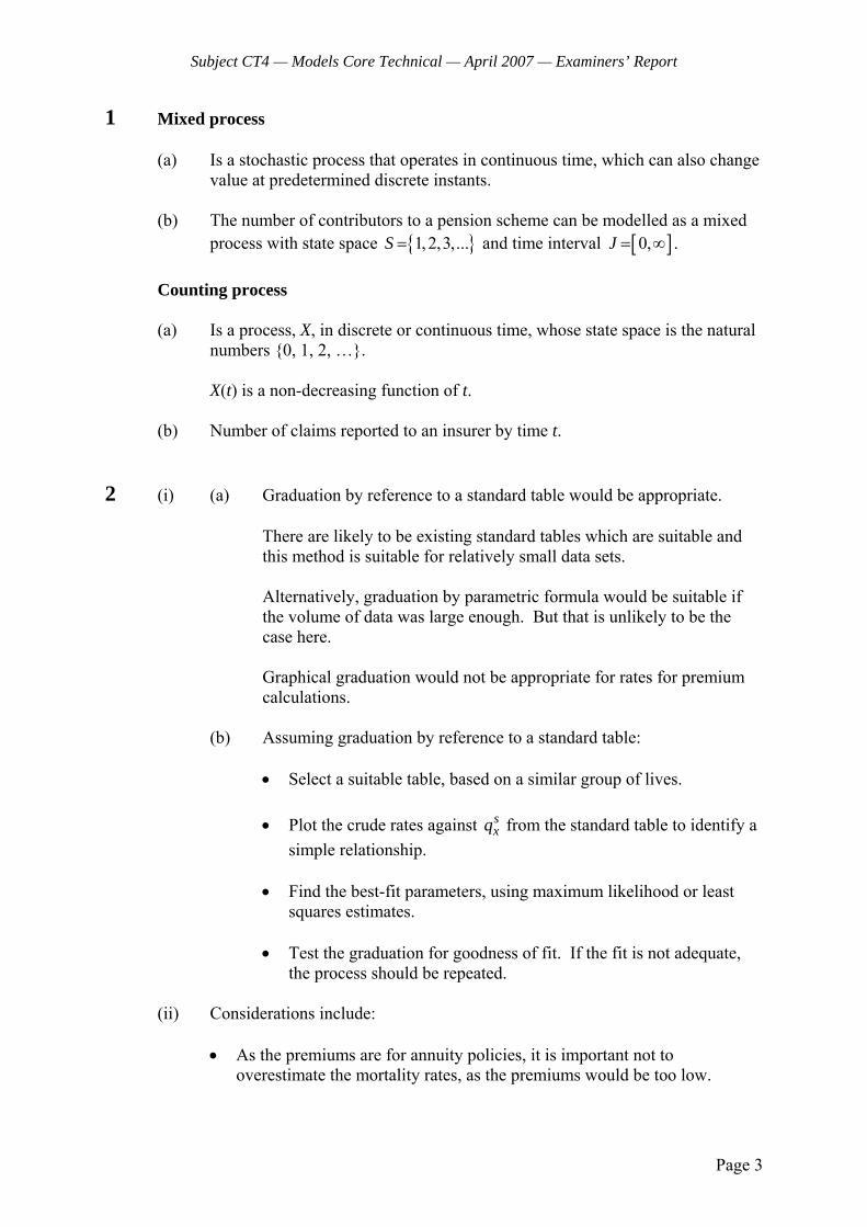
Subject CT4 — Models Core Technical — April 2007 — Examiners’ Report
Page 3
1 Mixed process (a) Is a stochastic process that operates in continuous time, which can also change
value at predetermined discrete instants. (b) The number of contributors to a pension scheme can be modelled as a mixed
process with state space { }1, 2,3,...S = and time interval [ ]0,J = ∞ . Counting process
(a) Is a process, X, in discrete or continuous time, whose state space is the natural
numbers {0, 1, 2, …}. X(t) is a non-decreasing function of t.
(b) Number of claims reported to an insurer by time t. 2 (i) (a) Graduation by reference to a standard table would be appropriate.
There are likely to be existing standard tables which are suitable and
this method is suitable for relatively small data sets.
Alternatively, graduation by parametric formula would be suitable if the volume of data was large enough. But that is unlikely to be the case here. Graphical graduation would not be appropriate for rates for premium calculations.
(b) Assuming graduation by reference to a standard table:
• Select a suitable table, based on a similar group of lives. • Plot the crude rates against s
xq from the standard table to identify a simple relationship.
• Find the best-fit parameters, using maximum likelihood or least
squares estimates. • Test the graduation for goodness of fit. If the fit is not adequate,
the process should be repeated. (ii) Considerations include:
• As the premiums are for annuity policies, it is important not to
overestimate the mortality rates, as the premiums would be too low.

Subject CT4 — Models Core Technical — April 2007 — Examiners’ Report
Page 4
• The rates will be based on current mortality; the company should also take into account expected future changes, especially any reductions in mortality rates.
• Premiums charged by other insurer: if rates are too high the company will
fail to attract business; if too low, it may attract too much, unprofitable business.
3 Clarify the purpose of the exercise. Why does the government want forecasts of
mortality? What is the period for which the forecast is wanted? Is it short (e.g. 5–10 years) or long (e.g. 50–70 years). Consult the existing literature on models for forecasting mortality, and speak to experts in this field of application. Consider using or adapting existing models which are employed in other countries. Establish what data are available (e.g. on past mortality trends in the country, preferably with deaths classified by age and cause of death). On the basis of what data are available, define the model you propose to use. If the data are simple and not detailed, then a complex model is not justified. Will a deterministic or a stochastic model be appropriate in this case? Identify suitable computer software to implement the model, or, if none exists, write a bespoke program. Debug the program or, if existing software is used, check that it performs the operations you intend it to do. Run the model and test the reasonableness of the output. Consider, for example, the forecast values of quantities such as the expectation of life at birth. Test the sensitivity of the results to changes in the input parameters. Analyse the output. Write a report documenting the results and the model and communicate the results and the output to the government of the small country.
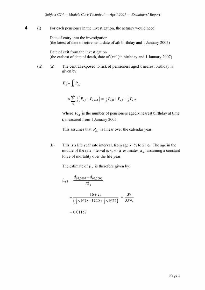
Subject CT4 — Models Core Technical — April 2007 — Examiners’ Report
Page 5
4 (i) For each pensioner in the investigation, the actuary would need: Date of entry into the investigation (the latest of date of retirement, date of xth birthday and 1 January 2005) Date of exit from the investigation (the earliest of date of death, date of (x+1)th birthday and 1 January 2007)
(ii) (a) The central exposed to risk of pensioners aged x nearest birthday is
given by
2
,0cx x tE P= ∫
( )1
1 1 1, , 1 ,0 ,1 ,22 2 2
0x t x t x x xP P P P P+≈ + = + +∑
Where ,x tP is the number of pensioners aged x nearest birthday at time
t, measured from 1 January 2005. This assumes that ,x tP is linear over the calendar year. (b) This is a life year rate interval, from age x-½ to x+½. The age in the
middle of the rate interval is x, so μ estimates xμ , assuming a constant force of mortality over the life year.
The estimate of xμ is therefore given by:
65,2005 65,200665
65ˆ
cd d
E
+μ =
( )1 1
2 2
16 23 3933701678 1720 1622
+= =
× + + ×
0.01157=
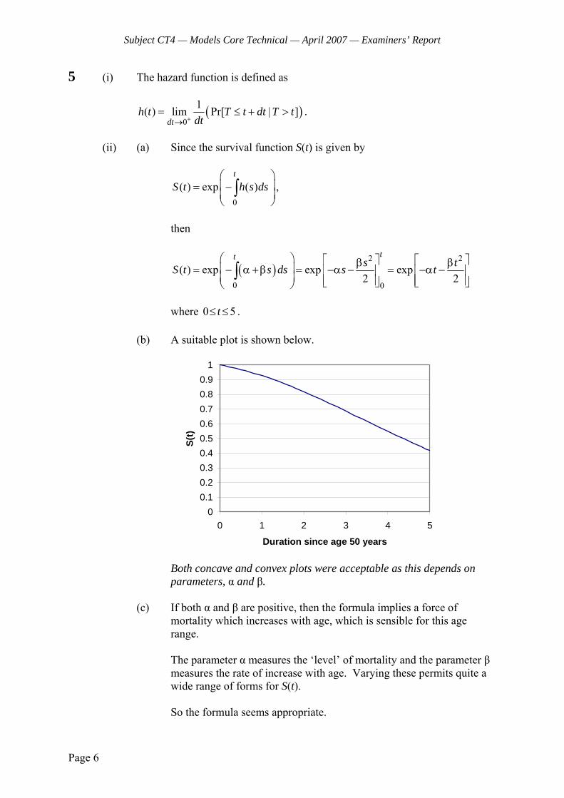
Subject CT4 — Models Core Technical — April 2007 — Examiners’ Report
Page 6
5 (i) The hazard function is defined as
( )0
1( ) lim Pr[ | ]dt
h t T t dt T tdt+→
= ≤ + > .
(ii) (a) Since the survival function S(t) is given by
0
( ) exp ( )t
S t h s ds⎛ ⎞⎜ ⎟= −⎜ ⎟⎝ ⎠∫ ,
then
( )2 2
0 0
( ) exp exp exp2 2
tt s tS t s ds s t⎛ ⎞ ⎡ ⎤ ⎡ ⎤β β⎜ ⎟= − α +β = −α − = −α −⎢ ⎥ ⎢ ⎥⎜ ⎟ ⎢ ⎥ ⎢ ⎥⎣ ⎦ ⎣ ⎦⎝ ⎠∫
where 0 5t≤ ≤ . (b) A suitable plot is shown below.
00.10.20.30.40.50.60.70.80.9
1
0 1 2 3 4 5
Duration since age 50 years
S(t)
Both concave and convex plots were acceptable as this depends on parameters, α and β.
(c) If both α and β are positive, then the formula implies a force of mortality which increases with age, which is sensible for this age range.
The parameter α measures the ‘level’ of mortality and the parameter β
measures the rate of increase with age. Varying these permits quite a wide range of forms for S(t).
So the formula seems appropriate.
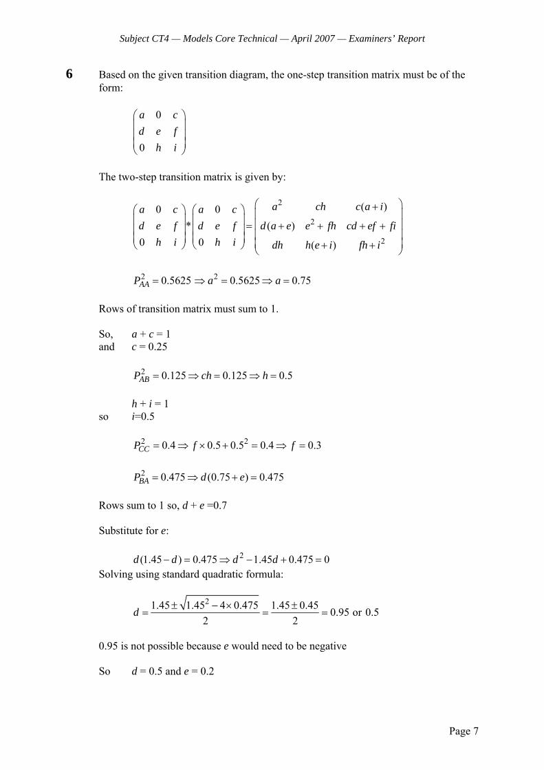
Subject CT4 — Models Core Technical — April 2007 — Examiners’ Report
Page 7
6 Based on the given transition diagram, the one-step transition matrix must be of the form:
0
0
a cd e f
h i
⎛ ⎞⎜ ⎟⎜ ⎟⎜ ⎟⎝ ⎠
The two-step transition matrix is given by:
2
2
2
( )0 0* ( )
0 0 ( )
a ch c a ia c a cd e f d e f d a e e fh cd ef fi
h i h i dh h e i fh i
⎛ ⎞+⎛ ⎞ ⎛ ⎞ ⎜ ⎟⎜ ⎟ ⎜ ⎟ ⎜ ⎟= + + + +⎜ ⎟ ⎜ ⎟ ⎜ ⎟⎜ ⎟ ⎜ ⎟ ⎜ ⎟+ +⎝ ⎠ ⎝ ⎠ ⎝ ⎠
2 0.5625AAP = 2 0.5625 0.75a a⇒ = ⇒ =
Rows of transition matrix must sum to 1. So, a + c = 1 and c = 0.25
2 0.125 0.125 0.5ABP ch h= ⇒ = ⇒ =
h + i = 1
so i=0.5
2 20.4 0.5 0.5 0.4 0.3CCP f f= ⇒ × + = ⇒ =
2 0.475 (0.75 ) 0.475BAP d e= ⇒ + =
Rows sum to 1 so, d + e =0.7
Substitute for e:
2(1.45 ) 0.475 1.45 0.475 0d d d d− = ⇒ − + = Solving using standard quadratic formula:
21.45 1.45 4 0.475 1.45 0.45 0.95 or 0.52 2
d ± − × ±= = =
0.95 is not possible because e would need to be negative
So d = 0.5 and e = 0.2

Subject CT4 — Models Core Technical — April 2007 — Examiners’ Report
Page 8
Transition matrix is:
0.75 0 0.250.5 0.2 0.30 0.5 0.5
⎛ ⎞⎜ ⎟⎜ ⎟⎜ ⎟⎝ ⎠
7 (i) Consider the sequence of the status of the first born child in each generation.
The state space consists of the four possible combinations of chromosomes: Female non-carrier (FN) or XX Female carrier (FC) or X*X Male non-sufferer (MN) or XY Male haemophiliac (MH) or X*Y
Using the assumption that there is an equal chance of either chromosome being inherited: • A female non-carrier will lead to a female non-carrier or male non-carrier.
• A female carrier may produce:
X*X, XX, X*Y, XY all with equal probability.
• A male non-sufferer will lead to female non-carrier or male non-carrier.
• A male haemophiliac may produce: X*X or XY (because his partner must provide an X) with equal probability.
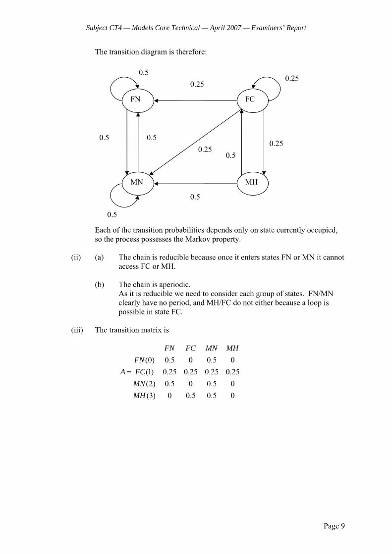
Subject CT4 — Models Core Technical — April 2007 — Examiners’ Report
Page 9
The transition diagram is therefore:
Each of the transition probabilities depends only on state currently occupied,
so the process possesses the Markov property. (ii) (a) The chain is reducible because once it enters states FN or MN it cannot
access FC or MH. (b) The chain is aperiodic. As it is reducible we need to consider each group of states. FN/MN
clearly have no period, and MH/FC do not either because a loop is possible in state FC.
(iii) The transition matrix is
(0) 0.5 0 0.5 0(1) 0.25 0.25 0.25 0.25(2) 0.5 0 0.5 0(3) 0 0.5 0.5 0
FN FC MN MHFN
A FCMNMH
=
FN FC
MN MH
0.5
0.5
0.5
0.5
0.5 0.25
0.25 0.25
0.25
0.5
Subject CT4 — Models Core Technical — April 2007 — Examiners’ Report
Page 10
The stationary distribution πmust satisfy:
0 0 1 20.5 0.25 0.5π = π + π + π
1 1 30.25 0.5π = π + π
2 0 1 2 30.5 0.25 0.5 0.5π = π + π + π + π
3 10.25π = π
So,
1 1 10.25 0.5 0.25π = π + × π
1 3 0⇒ π = π =
0 2 0.5⇒ π = π =
An alternative solution combines the states FN and MN to give a 3-state model. This was given credit.
8 (i) (a) Type I censoring is present for those lives still under observation at 31
December 2005 as the censoring times are known in advance.
(b) Interval censoring would be present if we only knew death occurred between check-ups. However, actual dates of death are known, so interval censoring is not present. Right censoring can be seen as a special case of interval censoring (for those censored before death, we know death occurs in the interval (ci, ∞) where ci is the censoring time for person i).
(c) Informative censoring is not likely to be present. The censoring of lives gives us no information about future lifetimes.
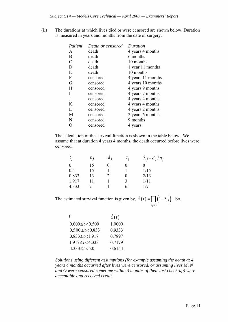
Subject CT4 — Models Core Technical — April 2007 — Examiners’ Report
Page 11
(ii) The durations at which lives died or were censored are shown below. Duration is measured in years and months from the date of surgery.
Patient Death or censored Duration A death 4 years 4 months B death 6 months C death 10 months D death 1 year 11 months E death 10 months F censored 4 years 11 months G censored 4 years 10 months H censored 4 years 9 months I censored 4 years 7 months J censored 4 years 4 months K censored 4 years 4 months L censored 4 years 2 months M censored 2 years 6 months N censored 9 months O censored 4 years
The calculation of the survival function is shown in the table below. We assume that at duration 4 years 4 months, the death occurred before lives were censored.
jt jn jd jc ˆ /j j jd nλ = 0 15 0 0 0 0.5 15 1 1 1/15 0.833 13 2 0 2/13 1.917 11 1 3 1/11 4.333 7 1 6 1/7
The estimated survival function is given by, ( ) ( )ˆ 1
j
jt t
S t≤
= −λ∏ . So,
t ( )S t 0.000 0.500t≤ < 1.0000 0.500 0.833t≤ < 0.9333 0.833 1.917t≤ < 0.7897 1.917 4.333t≤ < 0.7179 4.333 5.0t≤ < 0.6154
Solutions using different assumptions (for example assuming the death at 4 years 4 months occurred after lives were censored, or assuming lives M, N and O were censored sometime within 3 months of their last check-up) were acceptable and received credit.
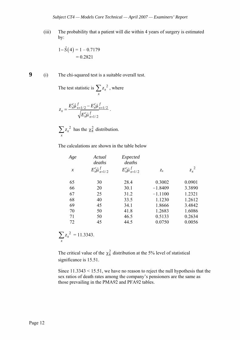
Subject CT4 — Models Core Technical — April 2007 — Examiners’ Report
Page 12
(iii) The probability that a patient will die within 4 years of surgery is estimated by:
( )ˆ1 4S− = 1 – 0.7179 = 0.2821
9 (i) The chi-squared test is a suitable overall test.
The test statistic is 2x
xz∑ , where
1/ 2 1/ 2
1/ 2
ˆ f fc cx xx x
x fcx x
E Ez
E+ +
+
μ − μ=
μ.
2
xx
z∑ has the 28χ distribution.
The calculations are shown in the table below
Age Actual Expected deaths deaths x 1/ 2ˆ fc
x xE +μ 1/ 2fc
x xE +μ zx 2
xz 65 30 28.4 0.3002 0.0901 66 20 30.1 -1.8409 3.3890 67 25 31.2 -1.1100 1.2321 68 40 33.5 1.1230 1.2612 69 45 34.1 1.8666 3.4842 70 50 41.8 1.2683 1.6086 71 50 46.5 0.5133 0.2634 72 45 44.5 0.0750 0.0056
2x
xz∑ = 11.3343.
The critical value of the 2
8χ distribution at the 5% level of statistical significance is 15.51. Since 11.3343 < 15.51, we have no reason to reject the null hypothesis that the sex ratios of death rates among the company’s pensioners are the same as those prevailing in the PMA92 and PFA92 tables.
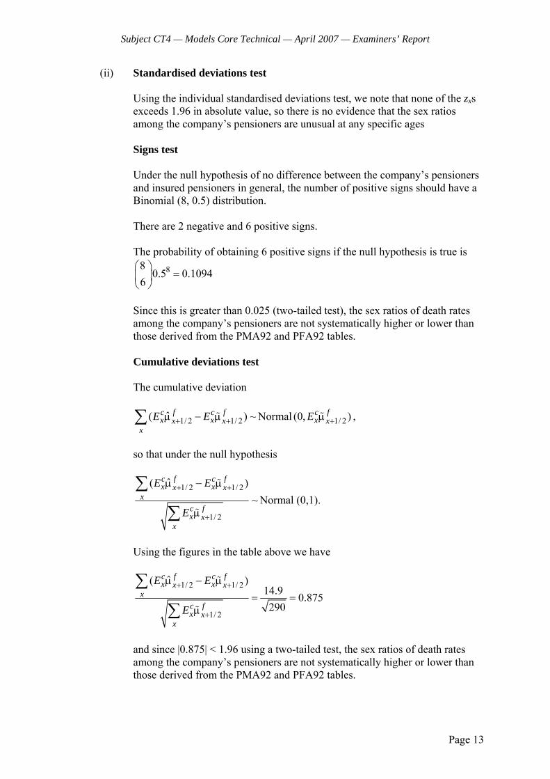
Subject CT4 — Models Core Technical — April 2007 — Examiners’ Report
Page 13
(ii) Standardised deviations test
Using the individual standardised deviations test, we note that none of the zxs exceeds 1.96 in absolute value, so there is no evidence that the sex ratios among the company’s pensioners are unusual at any specific ages Signs test Under the null hypothesis of no difference between the company’s pensioners and insured pensioners in general, the number of positive signs should have a Binomial (8, 0.5) distribution. There are 2 negative and 6 positive signs. The probability of obtaining 6 positive signs if the null hypothesis is true is
880.5 0.1094
6⎛ ⎞
=⎜ ⎟⎝ ⎠
Since this is greater than 0.025 (two-tailed test), the sex ratios of death rates among the company’s pensioners are not systematically higher or lower than those derived from the PMA92 and PFA92 tables. Cumulative deviations test The cumulative deviation
1/ 2 1/ 2ˆ( ) ~f fc cx xx x
xE E+ +μ − μ∑ Normal 1/ 2(0, )fc
x xE +μ ,
so that under the null hypothesis
1/ 2 1/ 2
1/ 2
ˆ( )~
f fc cx xx x
xfc
x xx
E E
E
+ +
+
μ − μ
μ
∑
∑Normal (0,1).
Using the figures in the table above we have
1/ 2 1/ 2
1/ 2
ˆ( )14.9 0.875290
f fc cx xx x
xfc
x xx
E E
E
+ +
+
μ − μ
= =μ
∑
∑
and since |0.875| < 1.96 using a two-tailed test, the sex ratios of death rates among the company’s pensioners are not systematically higher or lower than those derived from the PMA92 and PFA92 tables.
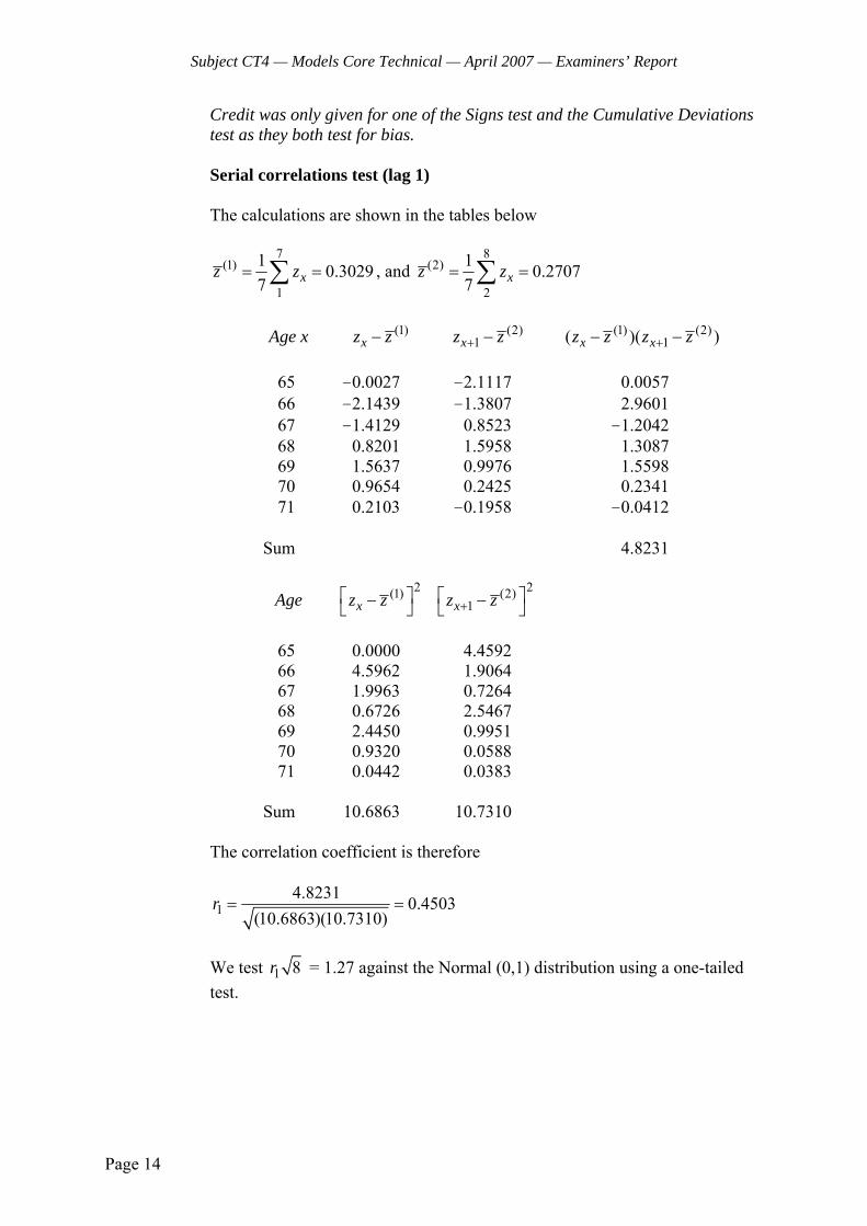
Subject CT4 — Models Core Technical — April 2007 — Examiners’ Report
Page 14
Credit was only given for one of the Signs test and the Cumulative Deviations test as they both test for bias. Serial correlations test (lag 1) The calculations are shown in the tables below
7(1)
1
1 0.30297 xz z= =∑ , and
8(2)
2
1 0.27077 xz z= =∑
Age x (1)
xz z− (2)1xz z+ − (1) (2)
1( )( )x xz z z z+− − 65 -0.0027 -2.1117 0.0057 66 -2.1439 -1.3807 2.9601 67 -1.4129 0.8523 -1.2042 68 0.8201 1.5958 1.3087 69 1.5637 0.9976 1.5598 70 0.9654 0.2425 0.2341 71 0.2103 -0.1958 -0.0412 Sum 4.8231
Age 2(1)
xz z⎡ ⎤−⎣ ⎦ 2(2)
1xz z+⎡ ⎤−⎣ ⎦
65 0.0000 4.4592 66 4.5962 1.9064 67 1.9963 0.7264 68 0.6726 2.5467 69 2.4450 0.9951 70 0.9320 0.0588 71 0.0442 0.0383 Sum 10.6863 10.7310
The correlation coefficient is therefore
14.8231 0.4503
(10.6863)(10.7310)r = =
We test 1 8r = 1.27 against the Normal (0,1) distribution using a one-tailed test.
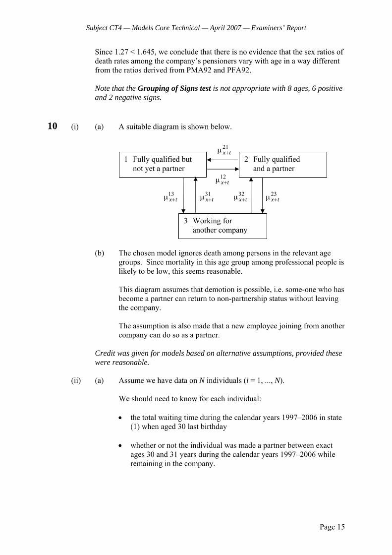
Subject CT4 — Models Core Technical — April 2007 — Examiners’ Report
Page 15
Since 1.27 < 1.645, we conclude that there is no evidence that the sex ratios of death rates among the company’s pensioners vary with age in a way different from the ratios derived from PMA92 and PFA92.
Note that the Grouping of Signs test is not appropriate with 8 ages, 6 positive and 2 negative signs.
10 (i) (a) A suitable diagram is shown below.
(b) The chosen model ignores death among persons in the relevant age
groups. Since mortality in this age group among professional people is likely to be low, this seems reasonable. This diagram assumes that demotion is possible, i.e. some-one who has become a partner can return to non-partnership status without leaving the company. The assumption is also made that a new employee joining from another company can do so as a partner.
Credit was given for models based on alternative assumptions, provided these were reasonable.
(ii) (a) Assume we have data on N individuals (i = 1, ..., N).
We should need to know for each individual: • the total waiting time during the calendar years 1997–2006 in state
(1) when aged 30 last birthday • whether or not the individual was made a partner between exact
ages 30 and 31 years during the calendar years 1997–2006 while remaining in the company.
2 Fully qualified and a partner
3 Working for another company
21x t+μ
12x t+μ
13x t+μ
1 Fully qualified but not yet a partner
31x t+μ 32
x t+μ 23x t+μ
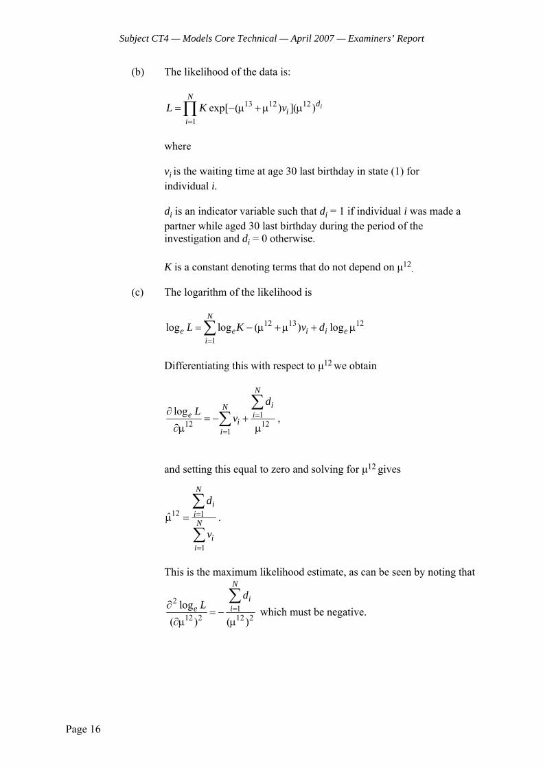
Subject CT4 — Models Core Technical — April 2007 — Examiners’ Report
Page 16
(b) The likelihood of the data is:
13 12 12
1exp[ ( ) ]( ) i
Nd
ii
L K v=
= − μ +μ μ∏
where vi is the waiting time at age 30 last birthday in state (1) for individual i. di is an indicator variable such that di = 1 if individual i was made a partner while aged 30 last birthday during the period of the investigation and di = 0 otherwise.
K is a constant denoting terms that do not depend on μ12
.
(c) The logarithm of the likelihood is
12 13 12
1log log ( ) log
N
e e i i ei
L K v d=
= − μ +μ + μ∑
Differentiating this with respect to μ12
we obtain
112 12
1
log
N
iNe i
ii
dL v =
=
∂= − +
∂μ μ
∑∑ ,
and setting this equal to zero and solving for μ12
gives
12 1
1
ˆ
N
iiN
ii
d
v
=
=
μ =∑
∑.
This is the maximum likelihood estimate, as can be seen by noting that
21
12 2 12 2log
( ) ( )
N
ie i
dL =∂= −
∂μ μ
∑ which must be negative.
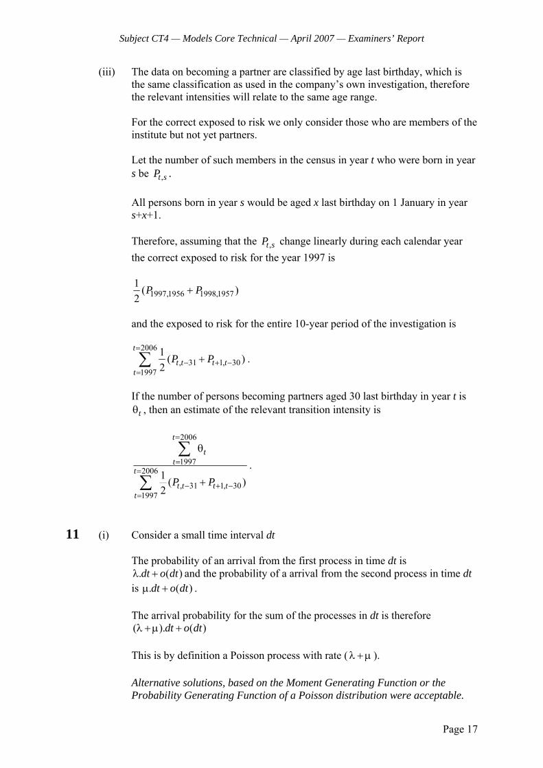
Subject CT4 — Models Core Technical — April 2007 — Examiners’ Report
Page 17
(iii) The data on becoming a partner are classified by age last birthday, which is the same classification as used in the company’s own investigation, therefore the relevant intensities will relate to the same age range.
For the correct exposed to risk we only consider those who are members of the institute but not yet partners. Let the number of such members in the census in year t who were born in year s be ,t sP . All persons born in year s would be aged x last birthday on 1 January in year s+x+1. Therefore, assuming that the ,t sP change linearly during each calendar year the correct exposed to risk for the year 1997 is
1997,1956 1998,19571 ( )2
P P+
and the exposed to risk for the entire 10-year period of the investigation is
2006
, 31 1, 301997
1 ( )2
t
t t t tt
P P=
− + −=
+∑ .
If the number of persons becoming partners aged 30 last birthday in year t is
tθ , then an estimate of the relevant transition intensity is
2006
19972006
, 31 1, 301997
1 ( )2
t
tt
t
t t t tt
P P
=
==
− + −=
θ
+
∑
∑.
11 (i) Consider a small time interval dt
The probability of an arrival from the first process in time dt is
. ( )dt o dtλ + and the probability of a arrival from the second process in time dt is . ( )dt o dtμ + . The arrival probability for the sum of the processes in dt is therefore ( ). ( )dt o dtλ +μ + This is by definition a Poisson process with rate (λ +μ ).
Alternative solutions, based on the Moment Generating Function or the Probability Generating Function of a Poisson distribution were acceptable.
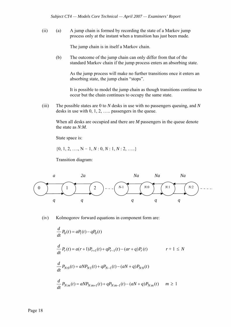
Subject CT4 — Models Core Technical — April 2007 — Examiners’ Report
Page 18
(ii) (a) A jump chain is formed by recording the state of a Markov jump process only at the instant when a transition has just been made.
The jump chain is in itself a Markov chain.
(b) The outcome of the jump chain can only differ from that of the
standard Markov chain if the jump process enters an absorbing state.
As the jump process will make no further transitions once it enters an absorbing state, the jump chain “stops”. It is possible to model the jump chain as though transitions continue to occur but the chain continues to occupy the same state.
(iii) The possible states are 0 to N desks in use with no passengers queuing, and N
desks in use with 0, 1, 2, ….. passengers in the queue.
When all desks are occupied and there are M passengers in the queue denote the state as N:M. State space is: {0, 1, 2, …., N - 1, N : 0, N : 1, N : 2, …..}
Transition diagram:
(iv) Kolmogorov forward equations in component form are:
0 1 0( ) ( ) ( )d P t aP t qP tdt
= −
1 1( ) ( 1) ( ) ( ) ( ) ( )r r r rd P t a r P t qP t ar q P tdt + −= + + − + r + 1 ≤ N
:0 :1 1 :0( ) ( ) ( ) ( ) ( )N N N Nd P t aNP t qP t aN q P tdt −= + − +
: : 1 : 1 :( ) ( ) ( ) ( ) ( )N m N m N m N md P t aNP t qP t aN q P tdt + −= + − + m ≥ 1
0 1 2 N-1 N:0 N:1 N:2
q q q q q
a 2a Na Na Na
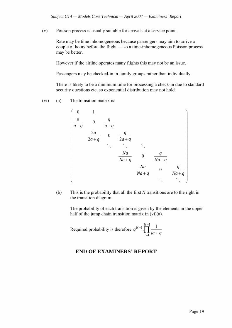
Subject CT4 — Models Core Technical — April 2007 — Examiners’ Report
Page 19
(v) Poisson process is usually suitable for arrivals at a service point. Rate may be time inhomogeneous because passengers may aim to arrive a couple of hours before the flight — so a time-inhomogeneous Poisson process may be better. However if the airline operates many flights this may not be an issue. Passengers may be checked-in in family groups rather than individually. There is likely to be a minimum time for processing a check-in due to standard security questions etc, so exponential distribution may not hold.
(vi) (a) The transition matrix is:
0 1
0
2 02 2
0
0
a qa q a q
a qa q a q
Na qNa q Na q
Na qNa q Na q
⎛ ⎞⎜ ⎟⎜ ⎟⎜ ⎟+ +⎜ ⎟⎜ ⎟⎜ ⎟+ +⎜ ⎟⎜ ⎟⎜ ⎟⎜ ⎟+ +⎜ ⎟⎜ ⎟⎜ ⎟+ +⎜ ⎟⎜ ⎟⎝ ⎠
(b) This is the probability that all the first N transitions are to the right in
the transition diagram.
The probability of each transition is given by the elements in the upper half of the jump chain transition matrix in (vi)(a).
Required probability is therefore 1
1
1
1.N
N
iq
ia q
−−
= +∏
END OF EXAMINERS’ REPORT

Faculty of Actuaries Institute of Actuaries
EXAMINATION
3 October 2007 (am)
Subject CT4 — Models Core Technical
Time allowed: Three hours
INSTRUCTIONS TO THE CANDIDATE
1. Enter all the candidate and examination details as requested on the front of your answer booklet.
2. You must not start writing your answers in the booklet until instructed to do so by the
supervisor. 3. Mark allocations are shown in brackets. 4. Attempt all 11 questions, beginning your answer to each question on a separate sheet. 5. Candidates should show calculations where this is appropriate.
Graph paper is not required for this paper.
AT THE END OF THE EXAMINATION
Hand in BOTH your answer booklet, with any additional sheets firmly attached, and this question paper.
In addition to this paper you should have available the 2002 edition of the Formulae and Tables and your own electronic calculator.
© Faculty of Actuaries CT4 S2007 © Institute of Actuaries

CT4 S2007—2
1 List the factors you would consider when assessing the suitability of an actuarial model for its purpose. [4]
2 A particular baker’s shop in a small town sells only one product: currant buns. These
currant buns are delicious and customers travel many miles to buy them. Unfortunately, the buns do not keep fresh and cannot be stored overnight.
The baker’s practice is to bake a certain number of buns, K, before the shop opens each morning, and then during the day to continue baking c buns per hour. He is concerned that: • he does not run out of buns during the day; and • the number of buns left over at the end of each day is as few as possible (i) Describe a model which would allow you to estimate the probability that the
baker will run out of buns. State any assumptions you make. [3]
(ii) Determine the relevant expression for the probability that the baker will run out of buns, in terms of K, c, and Bj, the number of buns bought by the day’s jth customer. [1]
[Total 4] 3 A no-claims discount system has 3 levels of discount: 0%, 25% and 50%. The rules
for moving between discount levels are: • After a claim-free year, move up to the next higher level or remain at the 50%
discount level. • After a year with one or more claims, move down to the next lower level or
remain at the 0% discount level. The long-run probability that a policyholder is in the maximum discount level is 0.75. Calculate the probability that a given policyholder has a claim-free year, assuming that this probability is constant. [5]
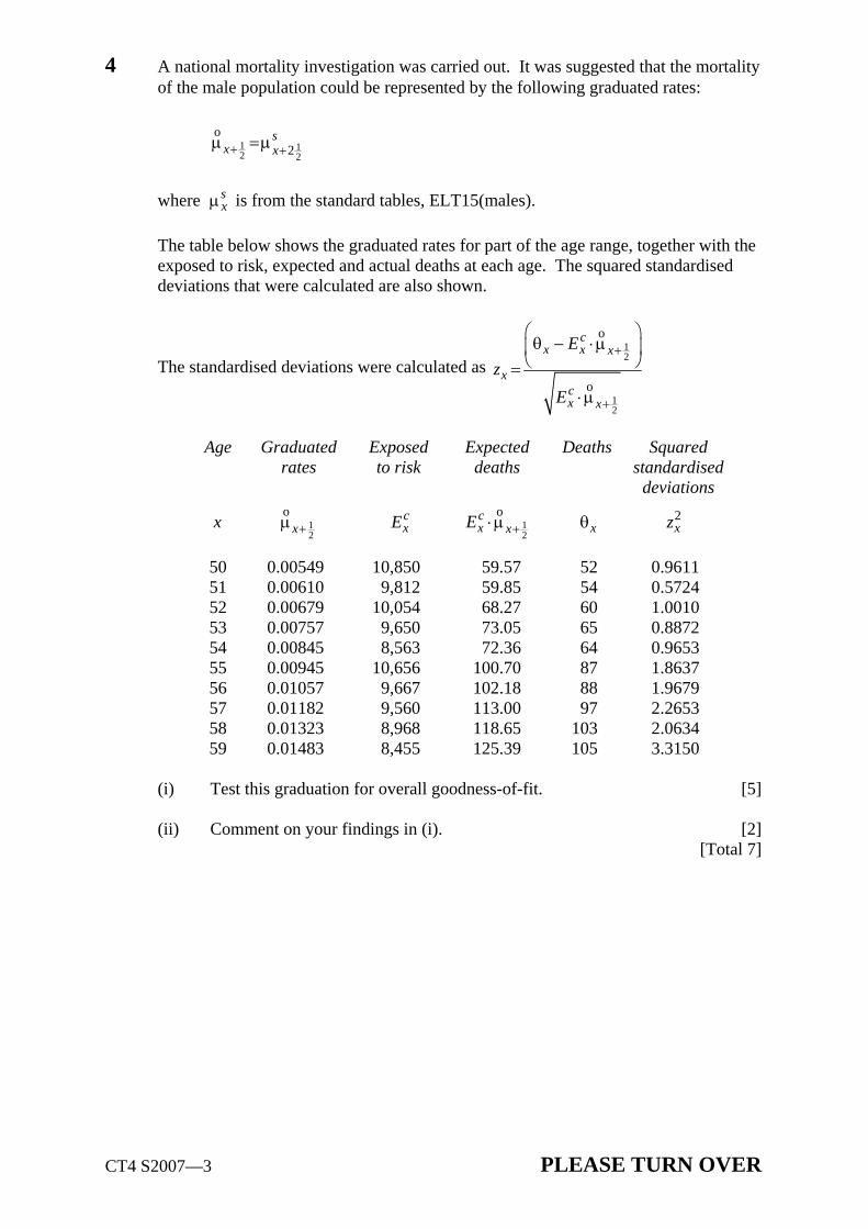
CT4 S2007—3 PLEASE TURN OVER
4 A national mortality investigation was carried out. It was suggested that the mortality of the male population could be represented by the following graduated rates:
1 12 2
o2
sx x+ +μ =μ
where s
xμ is from the standard tables, ELT15(males). The table below shows the graduated rates for part of the age range, together with the exposed to risk, expected and actual deaths at each age. The squared standardised deviations that were calculated are also shown.
The standardised deviations were calculated as 12
12
o
o
cx x x
xcx x
Ez
E
+
+
⎛ ⎞θ − ⋅μ⎜ ⎟⎝ ⎠=
⋅μ
Age Graduated
rates Exposed to risk
Expected deaths
Deaths Squared standardised
deviations
x 12
ox+μ c
xE 12
ocx xE +⋅μ xθ 2
xz
50 0.00549 10,850 59.57 52 0.9611 51 0.00610 9,812 59.85 54 0.5724 52 0.00679 10,054 68.27 60 1.0010 53 0.00757 9,650 73.05 65 0.8872 54 0.00845 8,563 72.36 64 0.9653 55 0.00945 10,656 100.70 87 1.8637 56 0.01057 9,667 102.18 88 1.9679 57 0.01182 9,560 113.00 97 2.2653 58 0.01323 8,968 118.65 103 2.0634 59 0.01483 8,455 125.39 105 3.3150
(i) Test this graduation for overall goodness-of-fit. [5]
(ii) Comment on your findings in (i). [2]
[Total 7]
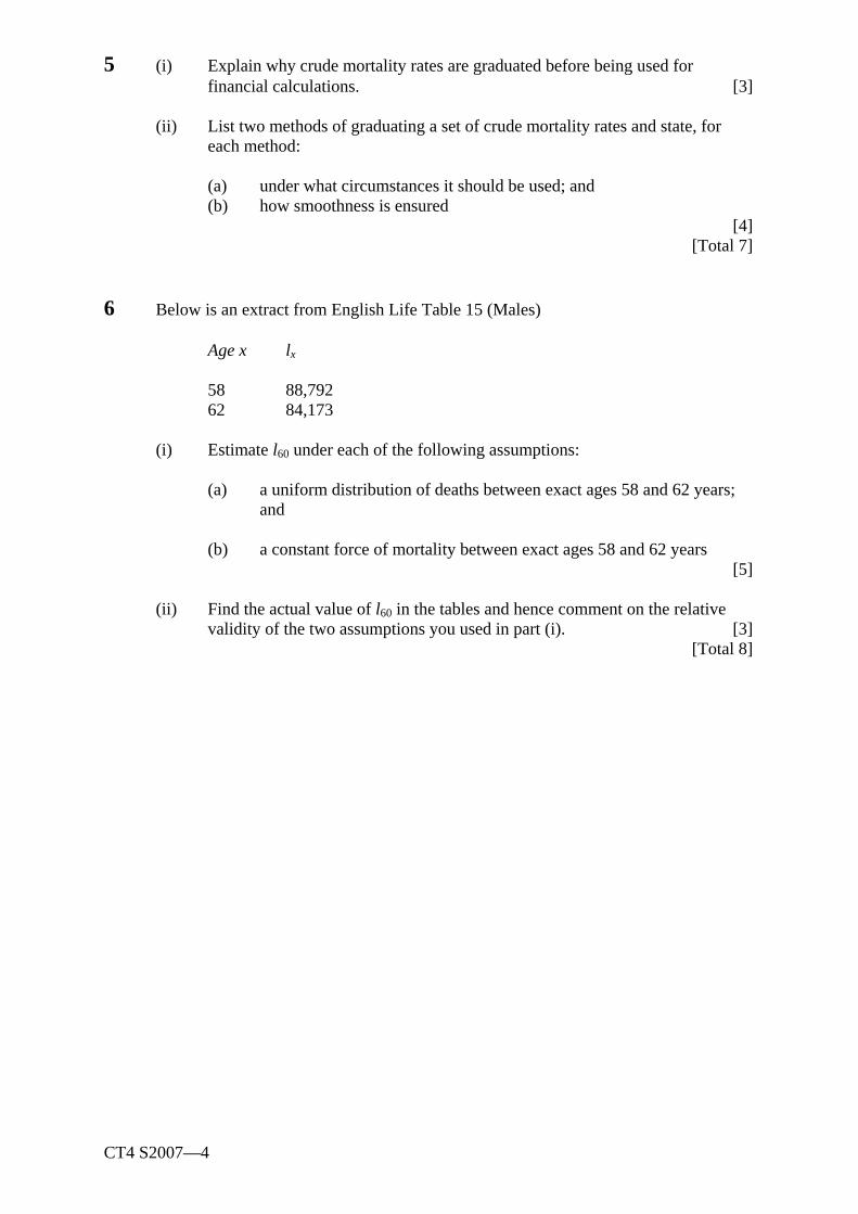
CT4 S2007—4
5 (i) Explain why crude mortality rates are graduated before being used for financial calculations. [3]
(ii) List two methods of graduating a set of crude mortality rates and state, for
each method: (a) under what circumstances it should be used; and (b) how smoothness is ensured [4] [Total 7] 6 Below is an extract from English Life Table 15 (Males)
Age x lx 58 88,792 62 84,173
(i) Estimate l60 under each of the following assumptions:
(a) a uniform distribution of deaths between exact ages 58 and 62 years;
and
(b) a constant force of mortality between exact ages 58 and 62 years [5]
(ii) Find the actual value of l60 in the tables and hence comment on the relative validity of the two assumptions you used in part (i). [3]
[Total 8]

CT4 S2007—5 PLEASE TURN OVER
7 In order to boost sales, a national newspaper in a European country wishes to compile a “fair play league table” for the country’s leading football clubs. On 1 December it undertakes a survey of all the players who play for these clubs, in which it collects the following data:
• number of games played by each player since the beginning of the season (the
football season in this country begins in September); and
• for each player who had been dismissed from the field of play between the beginning of the season and 1 December (inclusive), the number of games he had played before the game in which he was first dismissed
No games were played on 1 December. The statistic the newspaper proposes to use in order to construct its “fair play league table” is the probability that a player will not have been dismissed in any of his first 10 games. It plans to calculate this statistic for each of the 20 leading clubs. The following table shows the data collected for the players of the club which was top of the league on 1 December.
Player Total number Number of times Games of games played dismissed played before first dismissal 1 12 0 2 12 0 3 12 1 5 4 12 0 5 12 1 7 6 12 0 7 10 0 8 9 1 0 9 9 1 5 10 8 0 11 6 2 2 12 5 0 13 5 0 14 4 1 0 15 4 0
(i) (a) Explain how the Kaplan-Meier estimator can be used to estimate the
newspaper’s statistic from these data.
(b) Comment on the way in which censoring arises and on the type of censoring produced. [4]
(ii) Calculate the newspaper’s statistic using the data above. [4]
[Total 8]

CT4 S2007—6
8 (i) Describe the difference between the central exposed to risk and the initial exposed to risk. [2]
The following data come from an investigation of the mortality of participants in a dangerous sport during the calendar year 2005. Age x Number of lives aged x last Number of deaths birthday on: during 2005 to persons aged x last
1 January 2005 1 January 2006 birthday at death 22 150 160 20 23 160 155 25
(ii) (a) Estimate the initial exposed to risk at ages 22 and 23. (b) Hence estimate q22 and q23. [4]
Suppose that in this investigation, instead of aggregate data we had individual-level data on each person’s date of birth, date of death, and date of exit from observation (if exit was for reasons other than death). (iii) Explain how you would calculate the initial exposed-to-risk for lives aged 22
years last birthday. [4] [Total 10] 9 In a game of tennis, when the score is at “Deuce” the player winning the next point
holds “Advantage”. If a player holding “Advantage” wins the following point that player wins the game, but if that point is won by the other player the score returns to “Deuce”.
When Andrew plays tennis against Ben, the probability of Andrew winning any point is 0.6. Consider a particular game when the score is at “Deuce”.
(i) Show that the subsequent score in the game can be modelled as a Markov
Chain, specifying both:
(a) the state space; and (b) the transition matrix [3] (ii) State, with reasons, whether the chain is: (a) irreducible; and (b) aperiodic [2] (iii) Calculate the number of points which must be played before there is more than
a 90% chance of the game having been completed. [3] (iv) (a) Calculate the probability that Andrew wins the game. (b) Comment on your answer. [4] [Total 12]

CT4 S2007—7 PLEASE TURN OVER
10 (i) Compare the advantages and disadvantages of fully parametric models and the Cox regression model for assessing the impact of covariates on survival. [3]
You have been asked to investigate the impact of a set of covariates, including age, sex, smoking, region of residence, educational attainment and amount of exercise undertaken, on the risk of heart attack. Data are available from a prospective study which followed a set of several thousand persons from an initial interview until their first heart attack, or until their death from a cause other than a heart attack, or until 10 years had elapsed since the initial interview (whichever of these occurred first).
(ii) State the types of censoring present in this study, and explain how each arises.
[2]
(iii) Describe a criterion which would allow you to select those covariates which have a statistically significant effect on the risk of heart attack, when controlling the other covariates of the model. [4]
Suppose your final model is a Cox model which has three covariates: age (measured in age last birthday minus 50 at the initial interview), sex (male = 0, female = 1) and smoking (non-smoker = 0, smoker = 1), and that the estimated parameters are:
Age 0.01 Sex -0.4 Smoking 0.5 Sex x smoking -0.25
where “sex x smoking” is an additional covariate formed by multiplying the two covariates “sex” and “smoking”.
(iv) Describe the final model’s estimate of the effect of sex and of smoking
behaviour on the risk of heart attack. [3]
(v) Use the results of the model to determine how old a female smoker must be at the initial interview to have the same risk of heart attack as a male non-smoker aged 50 years at the initial interview. [3]
[Total 15]

CT4 S2007—8
11 The following data have been collected from observation of a three-state process in continuous time:
Total transitions to: State
occupied Total time
spent in state (hours)
State A State B State C
A 50 Not applicable 110 90 B 25 80 Not applicable 45 C 90 120 15 Not applicable
It is proposed to fit a Markov jump model to this data set. (i) (a) List all the parameters of the model. (b) Describe the assumptions underlying the model. [4] (ii) (a) Estimate the parameters of the model. (b) Give the estimated generator matrix. [4]
The following additional data in respect of secondary transitions were collected from
observation of the same process.
Triplet of successive transitions
Observed number of
triplets nijk
Triplet of successive transitions
Observed number of
triplets nijk
ABC 42 BCA 38 ABA 68 BCB 7 ACA 85 CAB 64 ACB 4 CAC 56 BAB 50 CBA 8 BAC 30 CBC 7
(iii) State the distribution of the number of transitions from state i to state j, given
the number of transitions out of state i. [1] (iv) Test the goodness-of-fit of the model by considering whether triplets of
successive transitions adhere to the distribution given in (iii). [5]
[Hint: Use the test statistic 2
2 ( )ijk
i j k
n EE−
χ =∑∑∑ where E is the expected
number of triplets under the distribution in (iii)] (v) Identify two other aspects of the appropriateness of the fitted model that could
be tested, stating suitable tests in each case. [2] (vi) Outline two methods for simulating the Markov jump process, without
performing any calculations. [4] [Total 20]
END OF PAPER

Faculty of Actuaries Institute of Actuaries
EXAMINATION
September 2007
Subject CT4 — Models Core Technical
EXAMINERS’ REPORT
Introduction The attached subject report has been written by the Principal Examiner with the aim of helping candidates. The questions and comments are based around Core Reading as the interpretation of the syllabus to which the examiners are working. They have however given credit for any alternative approach or interpretation which they consider to be reasonable. M A Stocker Chairman of the Board of Examiners December 2007
© Faculty of Actuaries © Institute of Actuaries

Subject CT4 — Models Core Technical — September 2007 — Examiners’ Report
Page 2
Comments Comments on solutions presented to individual questions for this September 2007 paper are given below and further comments may be written within in the solutions that follow. Q1 This straightforward bookwork question was not especially well answered. Q2 This was the most poorly answered question on the examination paper. Very few candidates recognised that the baker’s problem could be modelled using the compound Poisson process described in Unit 2 section 3.4 of the Core Reading. Q3 This was well answered, with many candidates scoring full marks. Q4 Although most candidates performed the chi-squared test correctly, few realised that when using this to test a graduation some degrees of freedom are lost, a fact which is clearly stated in the Core Reading in Unit 12, section 7.3. In part (ii) comments tended not to be related to the data in the question; rather they focused rather mechanically on the shortcomings of the chi-squared test. Q5 This straightforward bookwork question was well answered by many candidates. Q6 Most candidates obtained the correct numerical answers in part (i) of this question, but answers to part (ii) were rather sketchy and vague. Q7 This was more demanding than some previous questions on the Kaplan-Meier or Nelson-Aalen estimators, and the standard of the answers was lower than expected. Q8 This exposed-to-risk question was easier than many questions on the same topic in previous papers. Most candidates scored well on parts (i) and (ii), although few explained that the method relied on the assumption of a uniform distribution of deaths. Answers to part (iii) were less impressive and tended to lack detail. Some candidates couched their answers to this part in aggregate terms, despite the question clearly referring to individual-level data. Q9 Most candidates scored well on parts (i) and (ii). Common errors included the use of a three-state model (Deuce, Advantage and Game) which is inappropriate as the transition out of the state “Advantage” is ill-defined. Few candidates made attempts at parts (iii) and (iv) and several of these wrongly thought that part (iv) could be solved by finding the stationary distribution of the chain. Q10 Parts (i) and (iv) of this question tested knowledge of Unit 7, sections 2, 3 and 5 of the Core Reading, which has not been tested in previous CT4 examination papers. Perhaps because of this, many candidates gave very sketchy and vague answers. In part (ii), while most candidates spotted that Type I censoring was present, only a small minority also registered the existence of random censoring. In part (iii) few candidates correctly interpreted the sex x smoking interaction. Part (v) was well answered by most candidates. Q11 Many candidates only attempted parts (i) and (ii) of this question. The remainder was very poorly answered, with few candidates making serious attempts at part (vi), despite this being bookwork based on Core Reading, Unit 4, section 5.4.
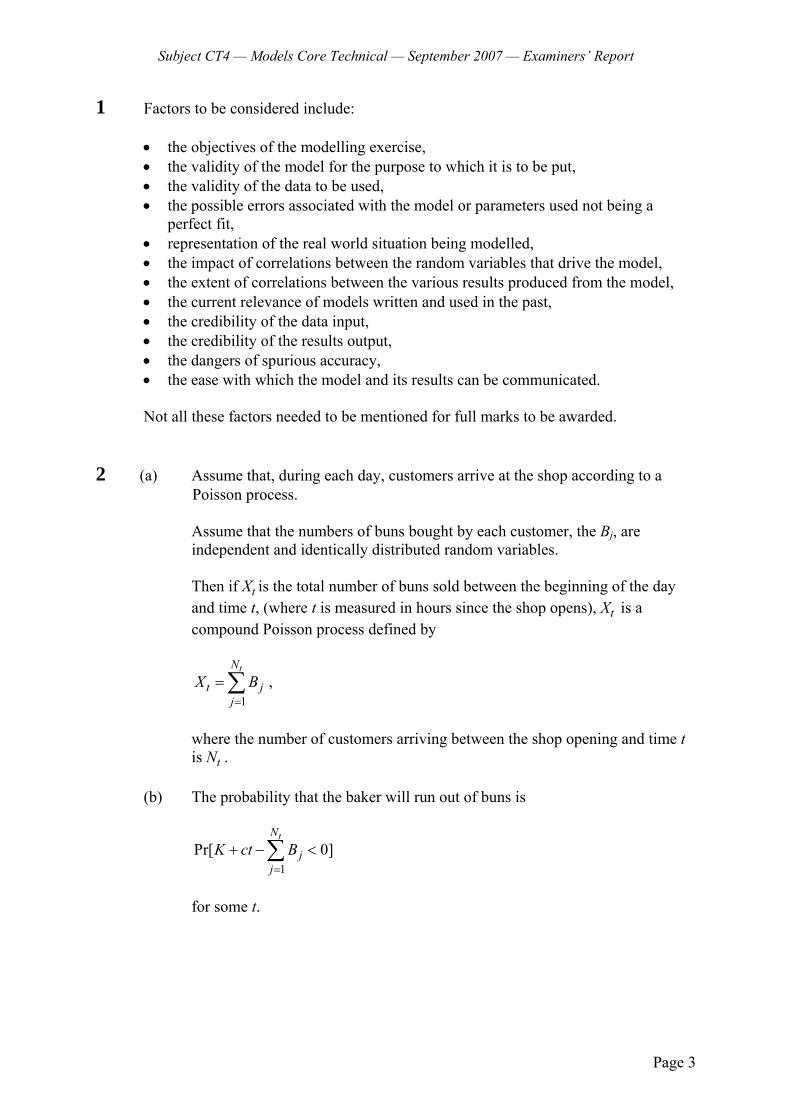
Subject CT4 — Models Core Technical — September 2007 — Examiners’ Report
Page 3
1 Factors to be considered include:
• the objectives of the modelling exercise, • the validity of the model for the purpose to which it is to be put, • the validity of the data to be used, • the possible errors associated with the model or parameters used not being a
perfect fit, • representation of the real world situation being modelled, • the impact of correlations between the random variables that drive the model, • the extent of correlations between the various results produced from the model, • the current relevance of models written and used in the past, • the credibility of the data input, • the credibility of the results output, • the dangers of spurious accuracy, • the ease with which the model and its results can be communicated.
Not all these factors needed to be mentioned for full marks to be awarded. 2 (a) Assume that, during each day, customers arrive at the shop according to a
Poisson process.
Assume that the numbers of buns bought by each customer, the Bj, are independent and identically distributed random variables.
Then if Xt is the total number of buns sold between the beginning of the day and time t, (where t is measured in hours since the shop opens), Xt is a compound Poisson process defined by
1
tN
t jj
X B=
=∑ ,
where the number of customers arriving between the shop opening and time t is Nt .
(b) The probability that the baker will run out of buns is
1Pr[ 0]
tN
jj
K ct B=
+ − <∑
for some t.
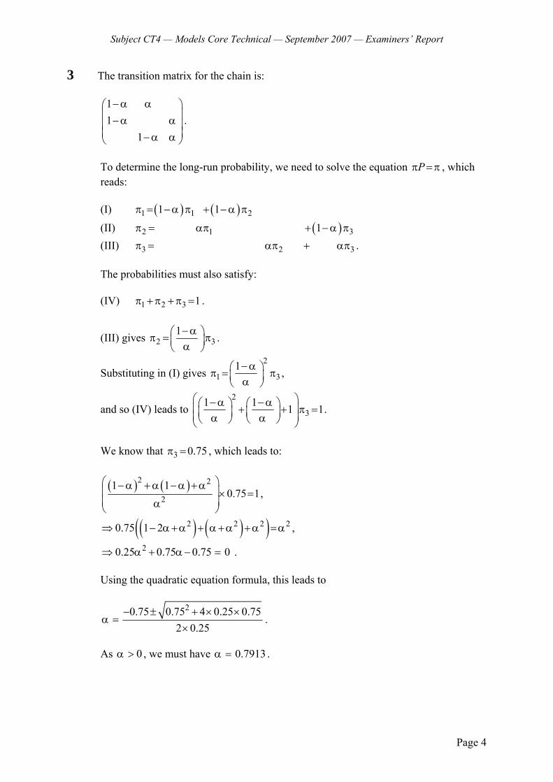
Subject CT4 — Models Core Technical — September 2007 — Examiners’ Report
Page 4
3 The transition matrix for the chain is:
11
1
−α α⎛ ⎞⎜ ⎟−α α⎜ ⎟⎜ ⎟−α α⎝ ⎠
.
To determine the long-run probability, we need to solve the equation Pπ =π , which reads: (I) ( ) ( )1 1 21 1π = −α π + −α π
(II) ( )2 1 31π = απ + −α π (III) 3 2 3π = απ + απ . The probabilities must also satisfy: (IV) 1 2 3 1π +π +π = .
(III) gives 2 31−α⎛ ⎞π = π⎜ ⎟α⎝ ⎠
.
Substituting in (I) gives 2
1 31−α⎛ ⎞π = π⎜ ⎟α⎝ ⎠
,
and so (IV) leads to 2
31 1 1 1
⎛ ⎞−α −α⎛ ⎞ ⎛ ⎞⎜ ⎟+ + π =⎜ ⎟ ⎜ ⎟⎜ ⎟α α⎝ ⎠ ⎝ ⎠⎝ ⎠.
We know that 3 0.75π = , which leads to:
( ) ( )2 2
21 1
0.75 1⎛ ⎞−α +α −α +α⎜ ⎟× =⎜ ⎟α⎝ ⎠
,
( ) ( )( )2 2 2 20.75 1 2⇒ − α+α + α+α +α =α ,
20.25 0.75 0.75 0⇒ α + α− = . Using the quadratic equation formula, this leads to
20.75 0.75 4 0.25 0.752 0.25
− ± + × ×α =
×.
As 0α > , we must have 0.7913α = .
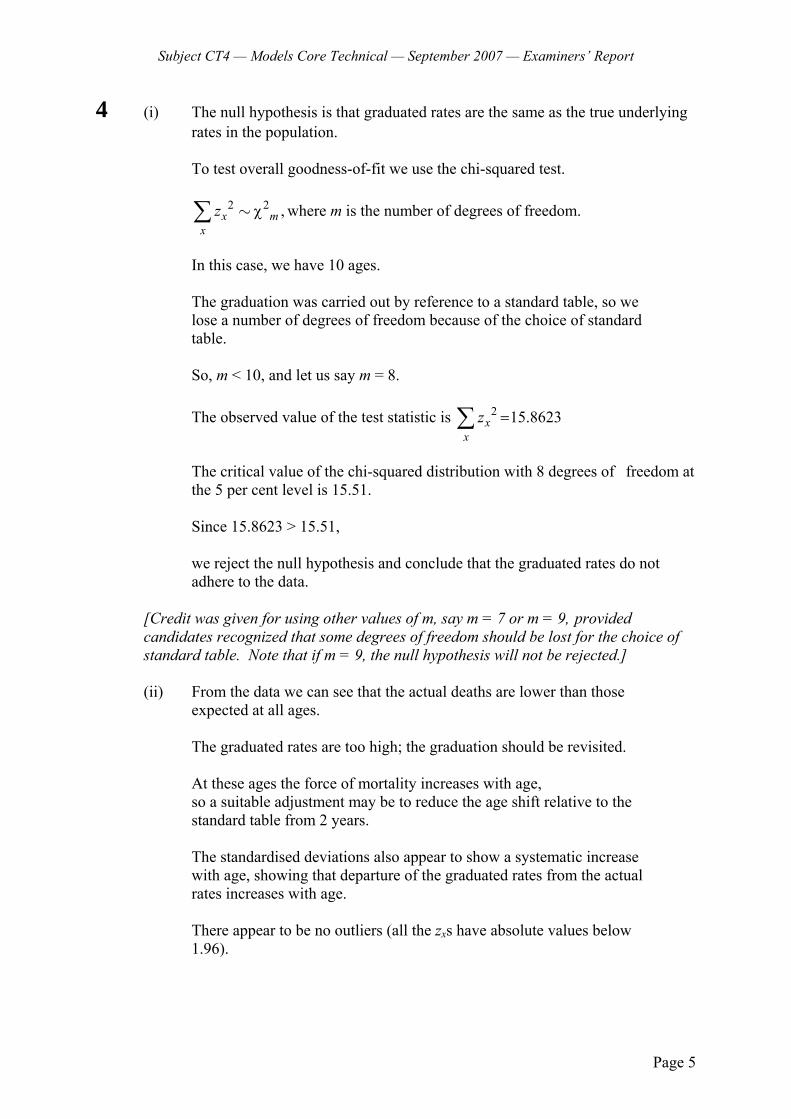
Subject CT4 — Models Core Technical — September 2007 — Examiners’ Report
Page 5
4 (i) The null hypothesis is that graduated rates are the same as the true underlying rates in the population.
To test overall goodness-of-fit we use the chi-squared test.
2 2
x mx
z χ∑ ∼ , where m is the number of degrees of freedom.
In this case, we have 10 ages. The graduation was carried out by reference to a standard table, so we lose a number of degrees of freedom because of the choice of standard table. So, m < 10, and let us say m = 8.
The observed value of the test statistic is 2 15.8623x
xz =∑
The critical value of the chi-squared distribution with 8 degrees of freedom at
the 5 per cent level is 15.51. Since 15.8623 > 15.51, we reject the null hypothesis and conclude that the graduated rates do not adhere to the data. [Credit was given for using other values of m, say m = 7 or m = 9, provided candidates recognized that some degrees of freedom should be lost for the choice of standard table. Note that if m = 9, the null hypothesis will not be rejected.]
(ii) From the data we can see that the actual deaths are lower than those expected at all ages.
The graduated rates are too high; the graduation should be revisited. At these ages the force of mortality increases with age, so a suitable adjustment may be to reduce the age shift relative to the standard table from 2 years. The standardised deviations also appear to show a systematic increase with age, showing that departure of the graduated rates from the actual rates increases with age. There appear to be no outliers (all the zxs have absolute values below 1.96).

Subject CT4 — Models Core Technical — September 2007 — Examiners’ Report
Page 6
5 (i) We assume that mortality rates progress smoothly with age.
Therefore a crude estimate at age x carries information about the rates at adjacent ages, and graduation allows us to use this fact to “improve” the estimate at age x by smoothing. This reduces the sampling errors at each age. It is desirable that financial quantities progress smoothly with age, as irregularities are hard to justify to clients.
(ii) Any two of the following three methods are acceptable:
By parametric formula: Should be used for large experiences, especially if the aim is to produce a standard table; Depends on a suitable formula being found which fits the data well. Provided the number of parameters is small, the resulting curve should be smooth. With reference to a standard table Should be used if a standard table for a class of lives similar to the experience is available, and the experience we are interested in does not provide much data. The standard table will be smooth, and provided the function linking the graduated rates to the rates in the standard table is simple, this smoothness will be “transferred to the graduated rates”. Graphical if a quick check is needed, or data are very scanty. The graduation should be tested for smoothness using the third differences of the graduated rates, which should be small in magnitude and progress regularly with age.
If the smoothness is unsatisfactory, the curve can be adjusted (“hand- polishing”) and the smoothness tested again.
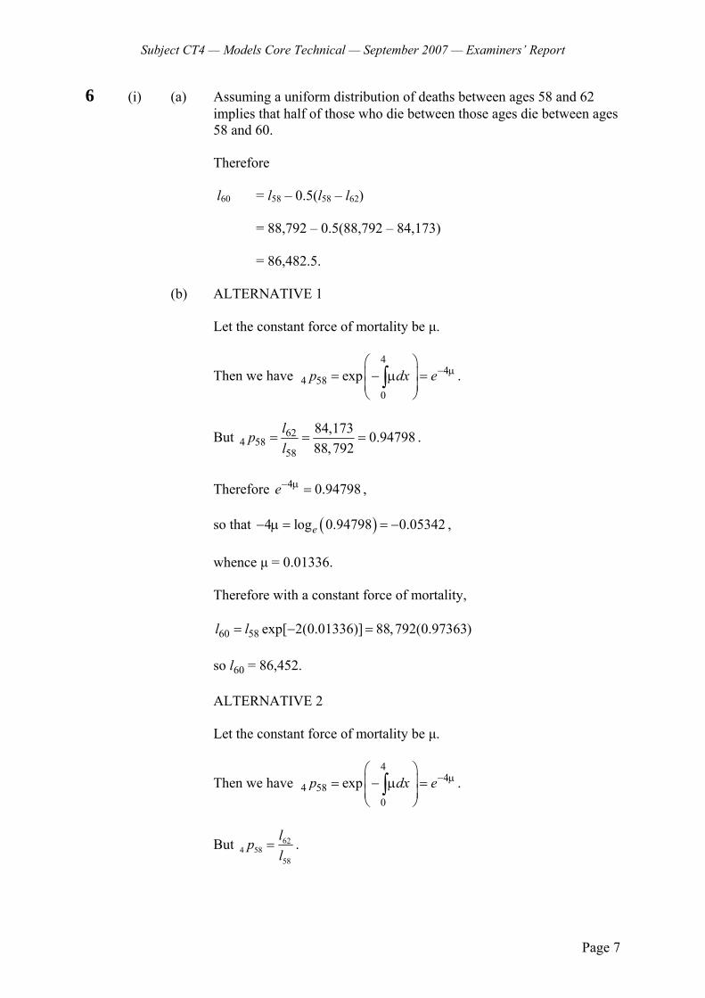
Subject CT4 — Models Core Technical — September 2007 — Examiners’ Report
Page 7
6 (i) (a) Assuming a uniform distribution of deaths between ages 58 and 62 implies that half of those who die between those ages die between ages 58 and 60.
Therefore
l60 = l58 – 0.5(l58 – l62)
= 88,792 – 0.5(88,792 – 84,173)
= 86,482.5.
(b) ALTERNATIVE 1 Let the constant force of mortality be μ.
Then we have 4
44 58
0
expp dx e− μ⎛ ⎞⎜ ⎟= − μ =⎜ ⎟⎝ ⎠∫ .
But 624 58
58
84,173 0.9479888,792
lpl
= = = .
Therefore 4 0.94798e− μ = ,
so that ( )4 log 0.94798 0.05342e− μ = = − , whence μ = 0.01336. Therefore with a constant force of mortality,
60 58 exp[ 2(0.01336)] 88,792(0.97363)l l= − = so l60 = 86,452.
ALTERNATIVE 2 Let the constant force of mortality be μ.
Then we have 4
44 58
0
expp dx e− μ⎛ ⎞⎜ ⎟= − μ =⎜ ⎟⎝ ⎠∫ .
But 624 58
58
lpl
= .
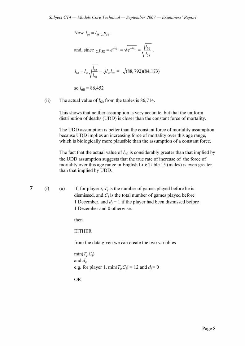
Subject CT4 — Models Core Technical — September 2007 — Examiners’ Report
Page 8
Now 60 58 2 58.l l p= .
and, since 2 4 622 58
58
lp e el
− μ − μ= = = ,
6260 58 58 62
58
ll l l ll
= = = (88,792)(84,173)
so l60 = 86,452 (ii) The actual value of l60 from the tables is 86,714.
This shows that neither assumption is very accurate, but that the uniform distribution of deaths (UDD) is closer than the constant force of mortality. The UDD assumption is better than the constant force of mortality assumption because UDD implies an increasing force of mortality over this age range, which is biologically more plausible than the assumption of a constant force. The fact that the actual value of l60 is considerably greater than that implied by the UDD assumption suggests that the true rate of increase of the force of mortality over this age range in English Life Table 15 (males) is even greater than that implied by UDD.
7 (i) (a) If, for player i, Ti is the number of games played before he is dismissed, and Ci is the total number of games played before 1 December, and di = 1 if the player had been dismissed before 1 December and 0 otherwise.
then EITHER from the data given we can create the two variables min(Ti,Ci) and di, e.g. for player 1, min(Ti,Ci) = 12 and di = 0
OR

Subject CT4 — Models Core Technical — September 2007 — Examiners’ Report
Page 9
The required data for the Kaplan-Meier estimator are therefore Player min(Ti,Ci) di
1 12 0 2 12 0 3 5 1 4 12 0 5 7 1 6 12 0 7 10 0 8 0 1 9 5 1 10 8 0 11 2 1 12 5 0 13 5 0
14 0 1 15 4 0
(b) Censoring in these data arises because not all players have been
dismissed before 1 December. Those players who have yet to be dismissed on that data are right-censored.
This censoring is random [NOT Type I], because the metric of “duration” is the number of games played since the start of the season, and this may vary from player to player.
(ii) ALTERNATIVE 1 (where censorings are assumed to occur immediately
before events)
tj Nj Dj Cj j
j
DN
1 j
j
DN
−
0 15 2 0 2/15 13/15 2 13 1 3 1/13 12/13 5 9 2 0 2/9 7/9 7 7 1 6 1/7 6/7
Then the Kaplan-Meier estimate of the survival function is
t ^( )S t
0≤ t < 2 0.8667 2≤ t < 5 0.8000 5≤ t < 7 0.6222 7≤ t < 12 0.5333
Therefore the value of the chosen statistic, ^
(10)S is 0.5333.
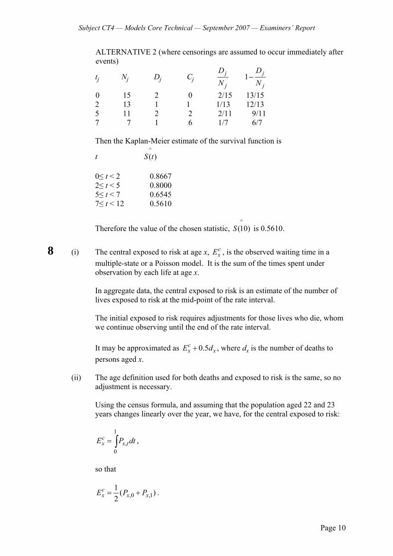
Subject CT4 — Models Core Technical — September 2007 — Examiners’ Report
Page 10
ALTERNATIVE 2 (where censorings are assumed to occur immediately after events)
tj Nj Dj Cj j
j
DN
1 j
j
DN
−
0 15 2 0 2/15 13/15 2 13 1 1 1/13 12/13 5 11 2 2 2/11 9/11 7 7 1 6 1/7 6/7 Then the Kaplan-Meier estimate of the survival function is
t ^( )S t
0≤ t < 2 0.8667 2≤ t < 5 0.8000 5≤ t < 7 0.6545 7≤ t < 12 0.5610
Therefore the value of the chosen statistic, ^
(10)S is 0.5610.
8 (i) The central exposed to risk at age x, cxE , is the observed waiting time in a
multiple-state or a Poisson model. It is the sum of the times spent under observation by each life at age x.
In aggregate data, the central exposed to risk is an estimate of the number of lives exposed to risk at the mid-point of the rate interval. The initial exposed to risk requires adjustments for those lives who die, whom we continue observing until the end of the rate interval. It may be approximated as 0.5c
x xE d+ , where dx is the number of deaths to persons aged x.
(ii) The age definition used for both deaths and exposed to risk is the same, so no
adjustment is necessary.
Using the census formula, and assuming that the population aged 22 and 23 years changes linearly over the year, we have, for the central exposed to risk:
1
,0
cx x tE P dt= ∫ ,
so that
,0 ,11 ( )2
cx x xE P P= + .
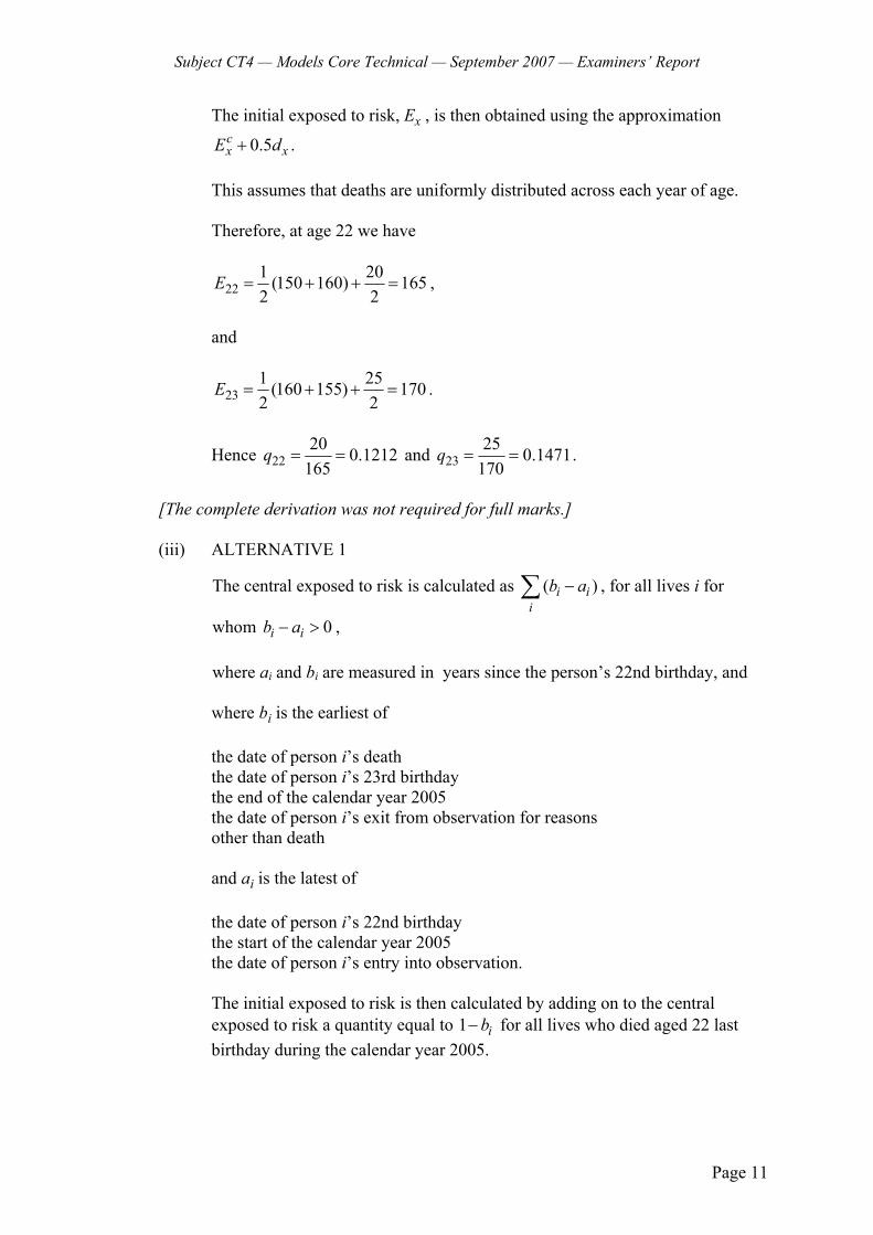
Subject CT4 — Models Core Technical — September 2007 — Examiners’ Report
Page 11
The initial exposed to risk, Ex , is then obtained using the approximation
0.5cx xE d+ .
This assumes that deaths are uniformly distributed across each year of age. Therefore, at age 22 we have
221 20(150 160) 1652 2
E = + + = ,
and
231 25(160 155) 1702 2
E = + + = .
Hence 2220 0.1212
165q = = and 23
25 0.1471170
q = = .
[The complete derivation was not required for full marks.] (iii) ALTERNATIVE 1
The central exposed to risk is calculated as ( )i ii
b a−∑ , for all lives i for
whom 0i ib a− > , where ai and bi are measured in years since the person’s 22nd birthday, and where bi is the earliest of the date of person i’s death the date of person i’s 23rd birthday the end of the calendar year 2005 the date of person i’s exit from observation for reasons other than death and ai is the latest of the date of person i’s 22nd birthday the start of the calendar year 2005 the date of person i’s entry into observation. The initial exposed to risk is then calculated by adding on to the central exposed to risk a quantity equal to 1 ib− for all lives who died aged 22 last birthday during the calendar year 2005.
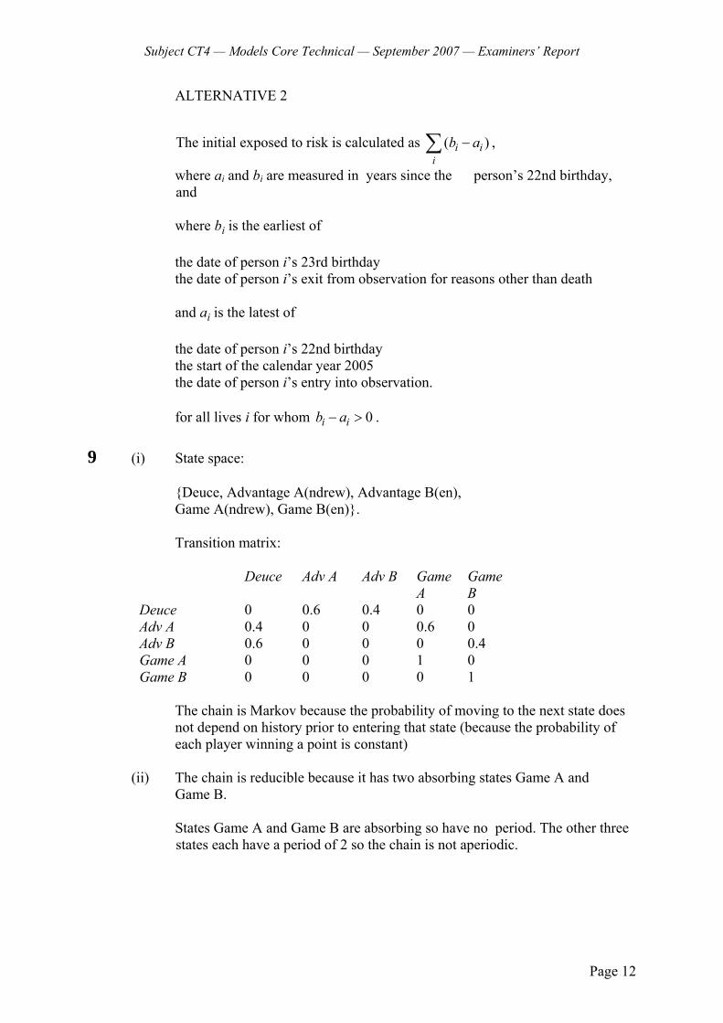
Subject CT4 — Models Core Technical — September 2007 — Examiners’ Report
Page 12
ALTERNATIVE 2
The initial exposed to risk is calculated as ( )i ii
b a−∑ ,
where ai and bi are measured in years since the person’s 22nd birthday, and
where bi is the earliest of the date of person i’s 23rd birthday the date of person i’s exit from observation for reasons other than death and ai is the latest of the date of person i’s 22nd birthday the start of the calendar year 2005 the date of person i’s entry into observation.
for all lives i for whom 0i ib a− > . 9 (i) State space:
{Deuce, Advantage A(ndrew), Advantage B(en), Game A(ndrew), Game B(en)}.
Transition matrix:
Deuce Adv A Adv B Game A
Game B
Deuce 0 0.6 0.4 0 0 Adv A 0.4 0 0 0.6 0 Adv B 0.6 0 0 0 0.4 Game A 0 0 0 1 0 Game B 0 0 0 0 1
The chain is Markov because the probability of moving to the next state does not depend on history prior to entering that state (because the probability of each player winning a point is constant)
(ii) The chain is reducible because it has two absorbing states Game A and
Game B. States Game A and Game B are absorbing so have no period. The other three states each have a period of 2 so the chain is not aperiodic.
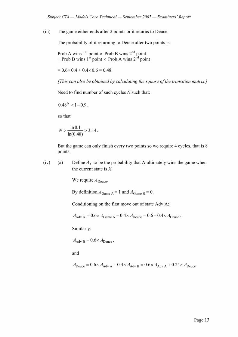
Subject CT4 — Models Core Technical — September 2007 — Examiners’ Report
Page 13
(iii) The game either ends after 2 points or it returns to Deuce.
The probability of it returning to Deuce after two points is:
Prob A wins 1st point × Prob B wins 2nd point + Prob B wins 1st point × Prob A wins 2nd point
= 0.6×0.4 + 0.4×0.6 = 0.48.
[This can also be obtained by calculating the square of the transition matrix.] Need to find number of such cycles N such that: 0.48 1 0.9N < − ,
so that
ln 0.1 3.14ln(0.48)
N > > .
But the game can only finish every two points so we require 4 cycles, that is 8 points.
(iv) (a) Define AX to be the probability that A ultimately wins the game when
the current state is X.
We require ADeuce. By definition AGame A = 1 and AGame B = 0. Conditioning on the first move out of state Adv A:
Adv A Game A Deuce Deuce0.6 0.4 0.6 0.4A A A A= × + × = + × . Similarly:
Adv B Deuce0.6A A= × , and
Deuce Adv A Adv B Adv A Deuce0.6 0.4 0.6 0.24A A A A A= × + × = × + × .
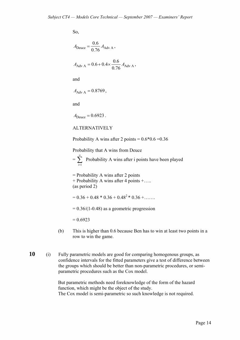
Subject CT4 — Models Core Technical — September 2007 — Examiners’ Report
Page 14
So,
Deuce Adv A0.60.76
A A= ,
Adv A Adv A0.60.6 0.40.76
A A= + × ,
and
Adv A 0.8769A = , and
Deuce 0.6923A = .
ALTERNATIVELY Probability A wins after 2 points = 0.6*0.6 =0.36 Probability that A wins from Deuce
= ∑∞
=1i
Probability A wins after i points have been played
= Probability A wins after 2 points + Probability A wins after 4 points +….. (as period 2) = 0.36 + 0.48 * 0.36 + 0.482 * 0.36 +……. = 0.36/(1-0.48) as a geometric progression = 0.6923
(b) This is higher than 0.6 because Ben has to win at least two points in a
row to win the game. 10 (i) Fully parametric models are good for comparing homogenous groups, as
confidence intervals for the fitted parameters give a test of difference between the groups which should be better than non-parametric procedures, or semi-parametric procedures such as the Cox model.
But parametric methods need foreknowledge of the form of the hazard function, which might be the object of the study. The Cox model is semi-parametric so such knowledge is not required.
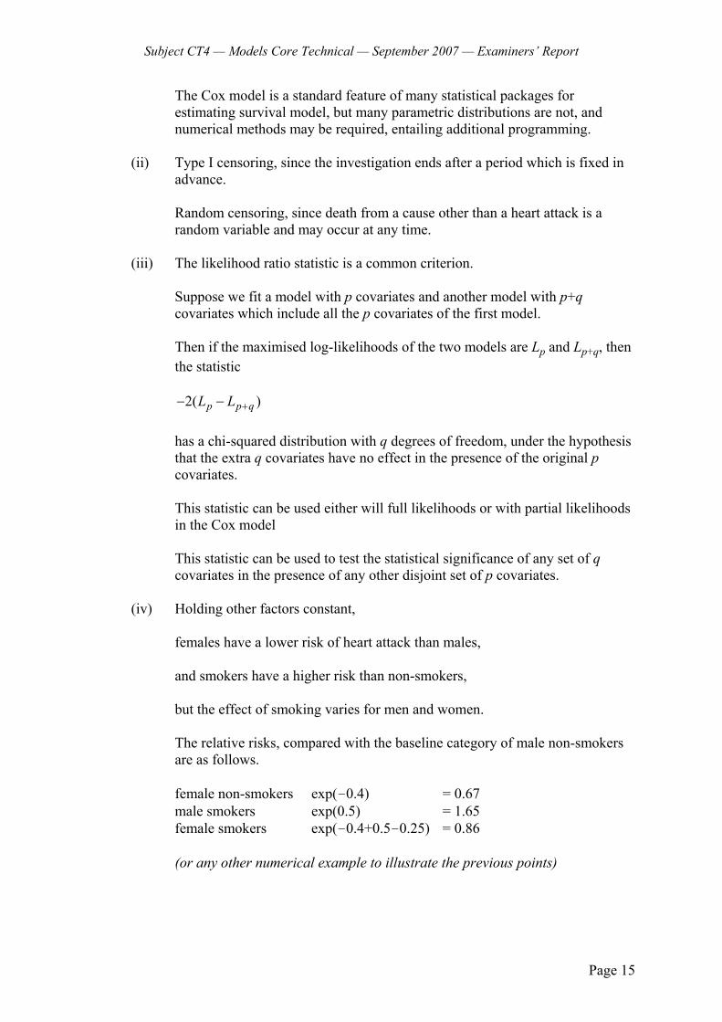
Subject CT4 — Models Core Technical — September 2007 — Examiners’ Report
Page 15
The Cox model is a standard feature of many statistical packages for estimating survival model, but many parametric distributions are not, and numerical methods may be required, entailing additional programming.
(ii) Type I censoring, since the investigation ends after a period which is fixed in
advance.
Random censoring, since death from a cause other than a heart attack is a random variable and may occur at any time.
(iii) The likelihood ratio statistic is a common criterion.
Suppose we fit a model with p covariates and another model with p+q covariates which include all the p covariates of the first model.
Then if the maximised log-likelihoods of the two models are Lp and Lp+q, then the statistic
2( )p p qL L +− − has a chi-squared distribution with q degrees of freedom, under the hypothesis that the extra q covariates have no effect in the presence of the original p covariates. This statistic can be used either will full likelihoods or with partial likelihoods in the Cox model This statistic can be used to test the statistical significance of any set of q covariates in the presence of any other disjoint set of p covariates.
(iv) Holding other factors constant,
females have a lower risk of heart attack than males, and smokers have a higher risk than non-smokers, but the effect of smoking varies for men and women.
The relative risks, compared with the baseline category of male non-smokers are as follows. female non-smokers exp(-0.4) = 0.67 male smokers exp(0.5) = 1.65 female smokers exp(-0.4+0.5-0.25) = 0.86 (or any other numerical example to illustrate the previous points)
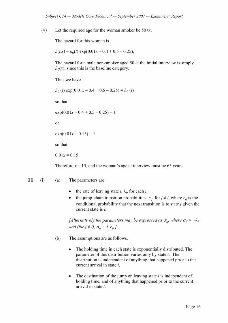
Subject CT4 — Models Core Technical — September 2007 — Examiners’ Report
Page 16
(v) Let the required age for the woman smoker be 50+x.
The hazard for this woman is h(t,x) = h0(t) exp(0.01x – 0.4 + 0.5 – 0.25), The hazard for a male non-smoker aged 50 at the initial interview is simply h0(x), since this is the baseline category. Thus we have h0 (t) exp(0.01x – 0.4 + 0.5 – 0.25) = h0 (t) so that exp(0.01x – 0.4 + 0.5 – 0.25) = 1 or exp(0.01x - 0.15) = 1 so that 0.01x = 0.15 Therefore x = 15, and the woman’s age at interview must be 65 years.
11 (i) (a) The parameters are:
• the rate of leaving state i, λi, for each i, • the jump-chain transition probabilities, rij, for j ≠ i, where rij is the
conditional probability that the next transition is to state j given the current state is i.
[Alternatively the parameters may be expressed as σij, where σii = -λi and (for j ≠ i), σij = λi rij.]
(b) The assumptions are as follows.
• The holding time in each state is exponentially distributed. The parameter of this distribution varies only by state i. The distribution is independent of anything that happened prior to the current arrival in state i.
• The destination of the jump on leaving state i is independent of
holding time, and of anything that happened prior to the current arrival in state i.
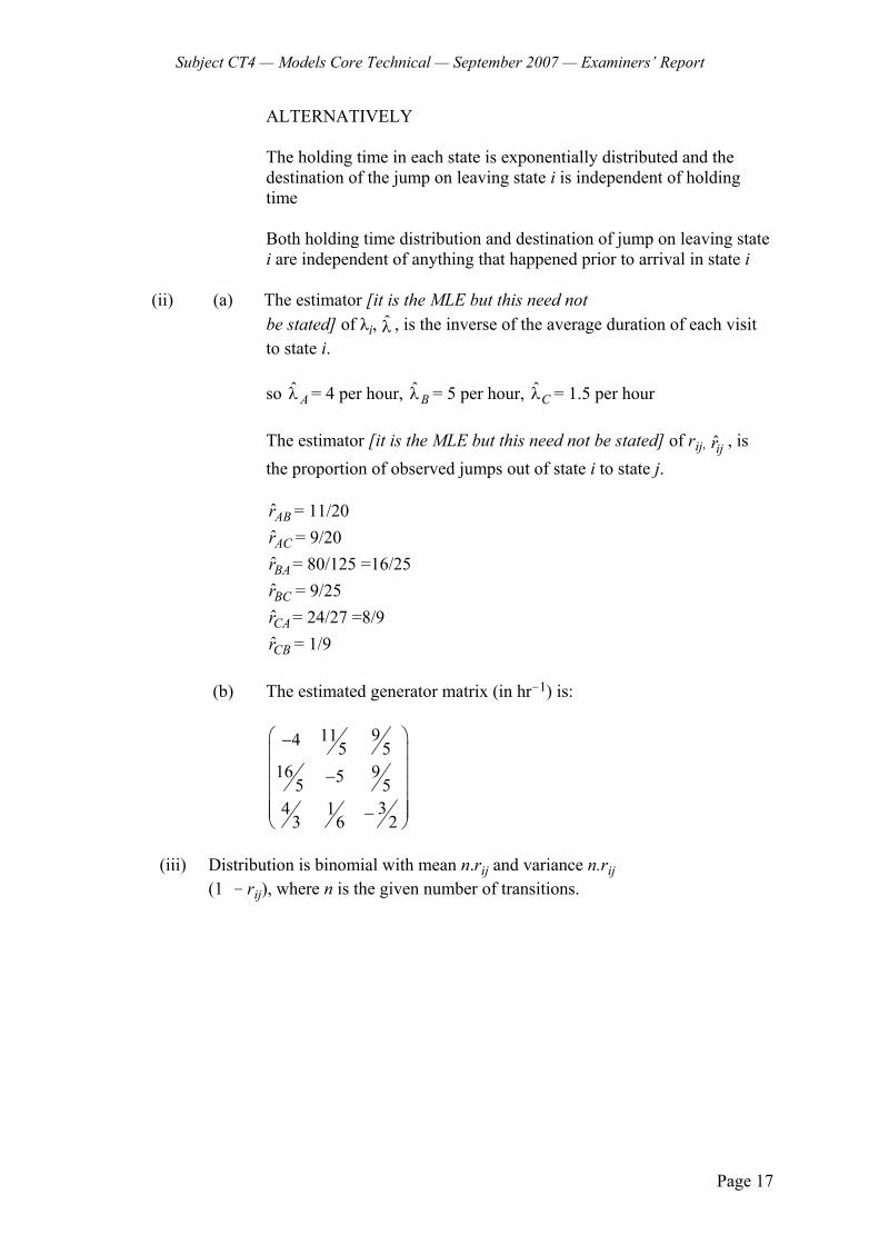
Subject CT4 — Models Core Technical — September 2007 — Examiners’ Report
Page 17
ALTERNATIVELY The holding time in each state is exponentially distributed and the destination of the jump on leaving state i is independent of holding time Both holding time distribution and destination of jump on leaving state i are independent of anything that happened prior to arrival in state i
(ii) (a) The estimator [it is the MLE but this need not be stated] of λi, λ , is the inverse of the average duration of each visit to state i.
so ˆ
Aλ = 4 per hour, ˆBλ = 5 per hour, ˆ
Cλ = 1.5 per hour
The estimator [it is the MLE but this need not be stated] of rij, ijr , is the proportion of observed jumps out of state i to state j.
ABr = 11/20
ACr = 9/20
BAr = 80/125 =16/25
BCr = 9/25
CAr = 24/27 =8/9
CBr = 1/9
(b) The estimated generator matrix (in hr-1) is:
9114 5 516 955 5
34 13 6 2
⎛ ⎞−⎜ ⎟⎜ ⎟−⎜ ⎟⎜ ⎟⎜ ⎟−⎝ ⎠
(iii) Distribution is binomial with mean n.rij and variance n.rij (1 - rij), where n is the given number of transitions.
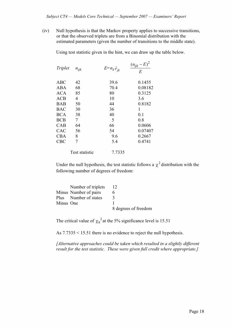
Subject CT4 — Models Core Technical — September 2007 — Examiners’ Report
Page 18
(iv) Null hypothesis is that the Markov property applies to successive transitions, or that the observed triplets are from a Binomial distribution with the estimated parameters (given the number of transitions to the middle state).
Using test statistic given in the hint, we can draw up the table below.
Triplet nijk E=nij ˆjkr 2( )ijkn E
E−
ABC 42 39.6 0.1455 ABA 68 70.4 0.08182 ACA 85 80 0.3125 ACB 4 10 3.6 BAB 50 44 0.8182 BAC 30 36 1 BCA 38 40 0.1 BCB 7 5 0.8 CAB 64 66 0.0606 CAC 56 54 0.07407 CBA 8 9.6 0.2667 CBC 7 5.4 0.4741
Test statistic 7.7335
Under the null hypothesis, the test statistic follows a 2χ distribution with the following number of degrees of freedom:
Number of triplets 12 Minus Number of pairs 6 Plus Number of states 3 Minus One 1 8 degrees of freedom The critical value of 2
8χ at the 5% significance level is 15.51 As 7.7335 < 15.51 there is no evidence to reject the null hypothesis. [Alternative approaches could be taken which resulted in a slightly different result for the test statistic. These were given full credit where appropriate.]
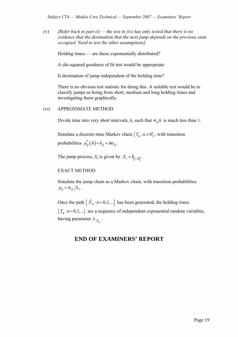
Subject CT4 — Models Core Technical — September 2007 — Examiners’ Report
Page 19
(v) [Refer back to part (i) — the test in (iv) has only tested that there is no evidence that the destination that the next jump depends on the previous state occupied. Need to test the other assumptions].
Holding times — are these exponentially distributed? A chi-squared goodness of fit test would be appropriate
Is destination of jump independent of the holding time? There is no obvious test statistic for doing this. A suitable test would be to classify jumps as being from short, medium and long holding times and investigating these graphically.
(vi) APPROXIMATE METHOD
Divide time into very short intervals, h, such that ijhσ is much less than 1. Simulate a discrete-time Markov chain { }: 0nY n ≥ , with transition
probabilities ( )*ij ij ijp h h=δ + σ .
The jump process, Xt is given by [ ]t t hX Y= .
EXACT METHOD Simulate the jump chain as a Markov chain, with transition probabilities
ij ij ip = σ λ . Once the path { }ˆ : 0,1,...nX n= has been generated, the holding times
{ }: 0,1,...nT n= are a sequence of independent exponential random variables, having parameter ˆ
nXλ .
END OF EXAMINERS’ REPORT

Faculty of Actuaries Institute of Actuaries
EXAMINATION
9 April 2008 (am)
Subject CT4 — Models Core Technical
Time allowed: Three hours
INSTRUCTIONS TO THE CANDIDATE
1. Enter all the candidate and examination details as requested on the front of your answer booklet.
2. You must not start writing your answers in the booklet until instructed to do so by the
supervisor. 3. Mark allocations are shown in brackets. 4. Attempt all 11 questions, beginning your answer to each question on a separate sheet. 5. Candidates should show calculations where this is appropriate.
Graph paper is not required for this paper.
AT THE END OF THE EXAMINATION
Hand in BOTH your answer booklet, with any additional sheets firmly attached, and this question paper.
In addition to this paper you should have available the 2002 edition of the Formulae and Tables and your own electronic calculator from the approved list.
© Faculty of Actuaries CT4 A2008 © Institute of Actuaries

CT4 A2008—2
1 List four factors in respect of which life insurance mortality statistics are often subdivided. [2]
2 Describe how smoothness is ensured when mortality rates are graduated using each of
the following methods: (a) fitting a parametric formula (b) graphical graduation [3] 3 (i) Define the following stochastic processes: (a) Poisson process (b) compound Poisson process [4] (ii) Identify the circumstances in which a compound Poisson process is also a
Poisson process. [1] [Total 5] 4 Describe the benefits and limitations of modelling in actuarial work. [6] 5 A survey of first marriage patterns among women in a remote population in central
Asia collected the following data for a sample of women:
• calendar year of birth • calendar year of first marriage
Data are also available about the population of never-married women on 1 January
each year, classified by age last birthday. You have been asked to estimate the intensity, xλ , of first marriage for women
aged x. (i) State the rate interval implied by the first marriages data. [1] (ii) Derive an appropriate exposed to risk which corresponds to the first marriages data. State any assumptions that you make. [4] (iii) Explain to what age x your estimate of xλ applies. State any assumptions that you make. [2] [Total 7]

CT4 A2008—3 PLEASE TURN OVER
6 An investigation was carried out into mortality rates among a certain class of female pensioners. Crude mortality rates were estimated by single years of age from ages
65–89 years last birthday inclusive. The investigators decided to ask an actuary to compare the crude rates with a standard table. They calculated the relevant standardised deviations, printed them out and sent them to the actuary.
Unfortunately, because of a printing error, the right-hand edge of the document
containing the standardised deviations failed to print properly. The actuary was unable to read the magnitude of the standardised deviations. However, the sign of each deviation was clear. This revealed that the crude mortality rates were higher than the standard table rates at ages 65–72 years and 75–84 years inclusive, but that the crude mortality rates were lower than the standard table rates at ages 73–74 years and 85–89 years inclusive.
The null hypothesis to be tested is that the crude mortality rates come from a
population with underlying mortality consistent with that in the standard table. (i) List two statistical tests of the null hypothesis which the actuary could carry
out on the basis of the information received. [1] (ii) Carry out both tests. For each test, state what feature of the experience it is
specifically testing, and give your conclusion. [10] [Total 11] 7 In a certain small country all listed companies are required to have their accounts
audited on an annual basis by one of the three authorised audit firms (A, B and C). The terms of engagement of each of the audit firms require that a minimum of two annual audits must be conducted by the newly appointed firm. Whenever a company is able to choose to change auditors, the likelihood that it will retain its auditors for a further year is (80%, 70%, 90%) where the current auditor is (A,B,C) respectively. If changing auditors a company is equally likely to choose either of the alternative firms.
(i) A company has just changed auditors to firm A. Calculate the expected
number of audits which will be undertaken before the company changes auditors again. [2]
(ii) Formulate a Markov chain which can be used to model the audit firm used by
a company, specifying: (a) the state space (b) the transition matrix [4] (iii) Calculate the expected proportion of companies using each audit firm in the
long term. [5] [Total 11]
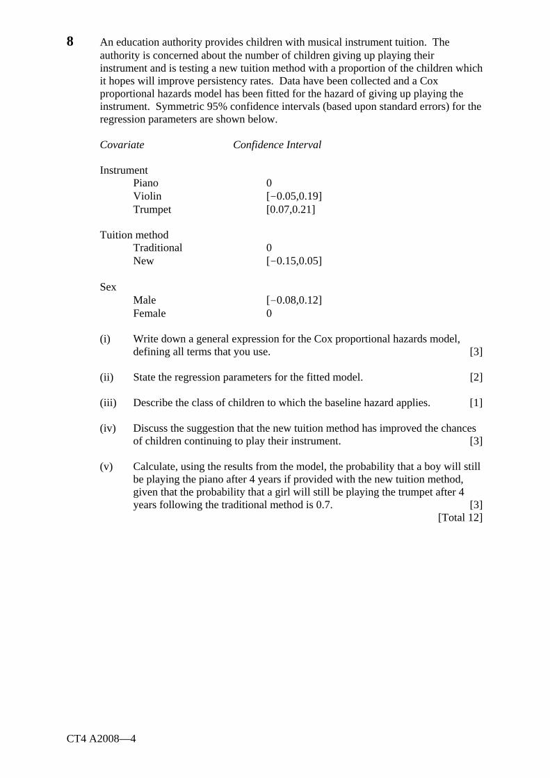
CT4 A2008—4
8 An education authority provides children with musical instrument tuition. The authority is concerned about the number of children giving up playing their instrument and is testing a new tuition method with a proportion of the children which it hopes will improve persistency rates. Data have been collected and a Cox proportional hazards model has been fitted for the hazard of giving up playing the instrument. Symmetric 95% confidence intervals (based upon standard errors) for the regression parameters are shown below.
Covariate Confidence Interval Instrument Piano 0 Violin [-0.05,0.19] Trumpet [0.07,0.21] Tuition method Traditional 0 New [-0.15,0.05] Sex Male [-0.08,0.12] Female 0 (i) Write down a general expression for the Cox proportional hazards model,
defining all terms that you use. [3] (ii) State the regression parameters for the fitted model. [2] (iii) Describe the class of children to which the baseline hazard applies. [1] (iv) Discuss the suggestion that the new tuition method has improved the chances
of children continuing to play their instrument. [3] (v) Calculate, using the results from the model, the probability that a boy will still
be playing the piano after 4 years if provided with the new tuition method, given that the probability that a girl will still be playing the trumpet after 4 years following the traditional method is 0.7. [3]
[Total 12]

CT4 A2008—5 PLEASE TURN OVER
9 An investigation into the mortality of patients following a specific type of major operation was undertaken. A sample of 10 patients was followed from the date of the operation until either they died, or they left the hospital where the operation was carried out, or a period of 30 days had elapsed (whichever of these events occurred first). The data on the 10 patients are given in the table below. Patient number Duration of Reason for observation observation (days) ceasing 1 2 Died 2 6 Died 3 12 Died 4 20 Left hospital 5 24 Left hospital 6 27 Died 7 30 Study ended 8 30 Study ended 9 30 Study ended 10 30 Study ended (i) State whether the following types of censoring are present in this
investigation. In each case give a reason for your answer. (a) Type I (b) Type II (c) Random [3] (ii) State, with a reason, whether the censoring in this investigation is likely to be
informative. [1] (iii) Calculate the value of the Kaplan-Meier estimate of the survival function at
duration 28 days. [5]
(iv) Write down the Kaplan-Meier estimate of the hazard of death at duration 8 days. [1]
(v) Sketch the Kaplan-Meier estimate of the survival function. [2] [Total 12]
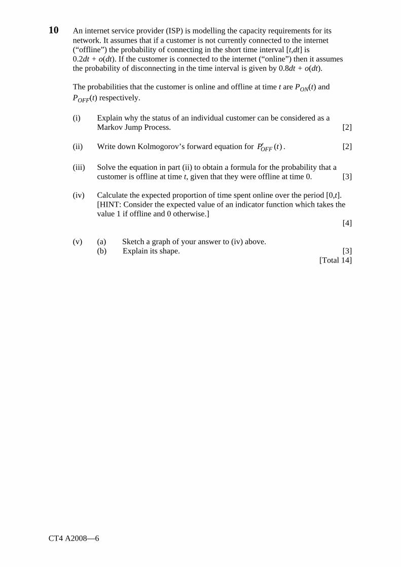
CT4 A2008—6
10 An internet service provider (ISP) is modelling the capacity requirements for its network. It assumes that if a customer is not currently connected to the internet (“offline”) the probability of connecting in the short time interval [t,dt] is
0.2dt + o(dt). If the customer is connected to the internet (“online”) then it assumes the probability of disconnecting in the time interval is given by 0.8dt + o(dt).
The probabilities that the customer is online and offline at time t are PON(t) and
POFF(t) respectively. (i) Explain why the status of an individual customer can be considered as a
Markov Jump Process. [2] (ii) Write down Kolmogorov’s forward equation for ( )OFFP t′ . [2] (iii) Solve the equation in part (ii) to obtain a formula for the probability that a
customer is offline at time t, given that they were offline at time 0. [3] (iv) Calculate the expected proportion of time spent online over the period [0,t]. [HINT: Consider the expected value of an indicator function which takes the
value 1 if offline and 0 otherwise.] [4]
(v) (a) Sketch a graph of your answer to (iv) above. (b) Explain its shape. [3] [Total 14]
CT4 A2008—7
11 An investigation was carried out into the relationship between sickness and mortality in an historical population of working class men. The investigation used a three-state model with the states:
1 Healthy 2 Sick 3 Dead Let the probability that a person in state i at time x will be in state j at time x+t be
ijt xp . Let the transition intensity at time x+t between any two states i and j be ij
x t+μ . (i) Draw a diagram showing the three states and the possible transitions between
them. [2] (ii) Show from first principles that
23 21 13 22 23t x t x x t t x x tp p p
t + +∂
= μ + μ∂
. [5]
(iii) Write down the likelihood of the data in the investigation in terms of the
transition rates and the waiting times in the Healthy and Sick states, under the assumption that the transition rates are constant. [3]
The investigation collected the following data:
• man-years in Healthy state 265 • man-years in Sick state 140 • number of transitions from Healthy to Sick 20 • number of transitions from Sick to Dead 40
(iv) Derive the maximum likelihood estimator of the transition rate from Sick to
Dead. [3] (v) Hence estimate: (a) the value of the constant transition rate from Sick to Dead (b) 95 per cent confidence intervals around this transition rate [4] [Total 17]
END OF PAPER

Faculty of Actuaries Institute of Actuaries
Subject CT4 — Models Core Technical
EXAMINERS’ REPORT
April 2008
Introduction The attached subject report has been written by the Principal Examiner with the aim of helping candidates. The questions and comments are based around Core Reading as the interpretation of the syllabus to which the examiners are working. They have however given credit for any alternative approach or interpretation which they consider to be reasonable. M A Stocker Chairman of the Board of Examiners June 2008
© Faculty of Actuaries © Institute of Actuaries

Subject CT4 — Models Core Technical — April 2008 — Examiners’ Report
Page 2
Comments Comments on solutions presented to individual questions for this April 2008 paper are given below. Question 1 This straightforward bookwork question was very well answered. Question 2 Answers to this question were disappointing. In part (a) many candidates did
not realise that smoothness is automatically ensured when graduating with a parametric formula with a small number of parameters. In part (b) many candidates presented descriptions of the method of graphical graduation, rather than answering the question which was set.
Question 3 Most candidates scored reasonably well on part (i), but few candidates could
state the conditions required for a compound Poisson process to be a Poisson process in part (ii).
Question 4 A reasonable attempt was made at this bookwork question by most candidates,
although few made sufficient distinct points to score close to full marks. Question 5 This exposed-to-risk question was quite well answered by many candidates,
who correctly identified the rate interval and the appropriate census-type formula. An encouraging number of candidates also recognised the need to adjust the age definition in order to ensure correspondence between the first marriages data and the exposed-to-risk data.
Question 6 Many candidates scored well on this question. Common errors were failure to
use (or incorrect use of) the continuity correction in the normal approximation to the signs test; calculating only the probability of 18 positive signs (rather than the probability of 18 or more signs) when using the exact binomial computation of the signs test; and calculating only the probability of 2 positive runs (rather than the probability of 2 or fewer positive runs) when using the exact computation of the grouping of signs test.
Question 7 Only a small proportion of candidates correctly answered part (i). In part (ii)
a very large number of candidates adopted a three-state solution to this problem, with state space {A, B, C}. Partial credit was given for this, and also for correctly following this three-state solution through in part (iii) to obtain the steady-state proportions of 3/11, 2/11 and 6/11 using auditors A, B and C respectively.
Question 8 This question was not as well answered as some others. Some candidates
failed to write the numerical values of the estimated parameters down in part (ii). There were few correct attempts at part (v). Many candidates simply calculated the ratio between the two hazards, which is incorrect. Others made unnecessary assumptions about the form of the baseline hazard (e.g. that it was constant).

Subject CT4 — Models Core Technical — April 2008 — Examiners’ Report
Page 3
Question 9 This straightforward calculation of the survival function was very well answered, apart from part (iv), in which only a handful of candidates realised that the Kaplan-Meier estimate of the hazard at any duration at which no event is observed to take place is 0. Given that the Kaplan-Meier estimate of the hazard is a step function, it is clear than this must be so. It was very encouraging to see the high proportion of sensible answers to part (ii). Credit was given in part (ii) to candidates who stated that the censoring was non-informative provided that the reason given was consistent with this statement.
Question 10 Few candidates scored highly on this question. Many candidates got no
further than part (ii). Although there were a fair number of attempts to solve the differential equation in part (iii), only a minority of candidates spotted that
( ) ( ) 1ON OFFP t P t+ = . Question 11 This question was very well answered. Many candidates provided
substantially correct answers to all parts, losing marks only for failure to include certain details in part (ii) (for example that we need to condition on the state occupied at time x+t); or for failing to point out that we need to substitute the estimated values from the data into the formula for the variance of 23μ in part (v).

Subject CT4 — Models Core Technical — April 2008 — Examiners’ Report
Page 4
1 Sex Age Type of policy Smoker/non-smoker Level of underwriting Duration in force Sales channel Policy size Known impairments Occupation 2 (a) Provided a formula with a small number of parameters is chosen the resulting graduation will be acceptably smooth. (b) The graduation should be tested for smoothness using the third differences of the graduated rates which should be small in magnitude and progress regularly.
A further iterative process, which involves manual adjustment of the graduation (called ‘hand-polishing’) is sometimes necessary to ensure smoothness.
Subject CT4 — Models Core Technical — April 2008 — Examiners’ Report
Page 5
3 (i) (a) EITHER A Poisson process with rate λ is a continuous-time integer-valued process Nt , t ≥ 0), with the following properties: N0 = 0 Nt has independent increments Nt has stationary increments
( )[ ( )][ ]
!
n t s
t st s eP N N n
n
−λ −λ −− = = s < t, n = 0, 1, 2…..
OR A Poisson process with rate λ is a continuous-time integer-valued process Nt , t ≥ 0), with the following properties: N0 = 0 [ 1] ( )t h tP N N h o h+ − = = λ + [ 0] 1 ( )t h tP N N h o h+ − = = −λ + [ 0,1] ( )t h tP N N o h+ − ≠ = (b) If Nt is a Poisson process on t ≥ 0 and Yi is a sequence of independent and identically distributed random variables then a compound Poisson process is defined by:
1
tN
t ii
X Y=
=∑
(ii) A compound Poisson process meets the conditions for being a Poisson process if Yi is an indicator function OR if each Yi is identically 1 (which is a special case of the indicator function)

Subject CT4 — Models Core Technical — April 2008 — Examiners’ Report
Page 6
4 Benefits Systems with long time frames can be studied in compressed time, for example the operation of a pension fund (or other suitable example). Complex systems with stochastic elements can be studied
Different future policies or possible actions can be compared.
In a model of a complex system we can usually get much better control over the experimental conditions so that we can reduce the variance of the results output from the model without upsetting their mean values Avoids costs and risks of making changes in the real world, so we can study impact of changing inputs before making decisions. Limitations
Model development requires a considerable investment of time and expertise. In a stochastic model, for any given set of inputs each run gives only estimates of a
model’s outputs. So to study the outputs for any given set of inputs, several independent runs of the model are needed.
Models can look impressive when run on a computer so that there is a danger that one gets lulled into a false sense of confidence.
If a model has not passed the tests of validity and verification its impressive output is a poor substitute for its ability to imitate its corresponding real world system.
Models rely heavily on the data input. If the data quality is poor or lacks credibility then the output from the model is likely to be flawed. It is important that the users of the model understand the model and the uses to which it can be safely put. There is a danger of using a model as a black box from which it is assumed that all results are valid without considering the appropriateness of using that model for the particular data input and the output expected.
It is not possible to include all future events in a model. For example a change in legislation could invalidate the results of a model, but may be impossible to predict when the model is constructed.
It may be difficult to interpret some of the outputs of the model. They may only be valid in relative, rather than absolute, terms. For example comparing the level of risk of the outputs associated with different inputs.

Subject CT4 — Models Core Technical — April 2008 — Examiners’ Report
Page 7
5 (i) Calendar year rate interval starting on 1 January each year. (ii) The first marriages data may be described as mx = number of first marriages, age x on the birthday in the
calendar year of marriage, during a defined period of investigation of length N years
A definition of the population data which is compatible with these data on first marriages is
Px,t = number of lives under observation at time t since the start of the
investigation who were aged x next birthday on the 1 January immediately preceding t
Since we follow each cohort of lives through each calendar year, this exposed to risk is
,0
Ncx x tE P dt= ∫
which may be approximated as
1
, 1, 10
1( )2
Ncx x t x tE P P
−
+ += +∑
(where the summation considers just integer values of t).
This assumes that the population varies linearly across the calendar year. However, we have data classified by age last birthday so we need to make a further adjustment. If the number of lives aged x last birthday on 1 January in year t is Px,t* then Px,t = Px-1,t*
and an appropriate exposed to risk in terms of the data we have is
* *1, , 1
1( )2
K Ncx x t x t
t KE P P
+
− +=
= +∑ .
Subject CT4 — Models Core Technical — April 2008 — Examiners’ Report
Page 8
(iii) The age range at the start of the rate interval is (x–1, x) exact. So, assuming that birthdays are uniformly distributed across the calendar year the average age at the start of the rate interval is x–½ and the average age in the middle of the rate interval is x. Therefore the estimate of xλ applies to age x. 6 (i) Since we do not know the values of the rates in the crude experience but only the signs of the deviations the tests we can carry out are limited. We can, however, perform the signs test and the grouping of signs test. (ii) The signs test looks for overall bias. We have 25 ages, and at 18 of these the crude rates exceed the standard table rates (i.e. we have positive deviations) If the null hypothesis is true, then the observed number of positive deviations, P, will be such that P ~ Binomial (25, ½). EITHER We use the normal approximation to the Binomial distribution because we have a large number of ages (>20) This means that, approximately, P ~ Normal (12.5, 6.25). The z-score associated with the probability of getting 18 positive deviations if the null hypothesis is true is, therefore
17.5 12.5 5 2.002.56.25
− −= = − .
(using a continuity correction). We use a two-tailed test, since both an excess of positive and an excess of negative deviations are of interest. Using a 5 % significance level, we have -2.00 < -1.96. This means we have just sufficient evidence to reject the null hypothesis.

Subject CT4 — Models Core Technical — April 2008 — Examiners’ Report
Page 9
OR Using the Binomial exactly we have
Pr[j positive deviations] = 25250.5
j⎛ ⎞⎜ ⎟⎝ ⎠
.
So that the probability of obtaining 18 or more positive
deviations is25
25
18
250.5
j j=
⎛ ⎞⎜ ⎟⎝ ⎠
∑ .
This is equal to (1 + 25 + 300 + 2,300 + 12,650 + 53,130 + 177,100 + 480,700) × 0.0000000298 = 0.02164. We apply a 2-tailed test, so we reject the null hypothesis at the 5% level if this is less than 0.025 Since 0.02164 < 0.025 we reject the null hypothesis. The grouping of signs test looks for long runs or clumps of ages with the same sign, indicating that the crude experience is different from the standard experience over a substantial age range. The number of runs of positive signs is 2 (65–72 years and 75–84 years). We have 25 ages and 18 positive signs in total, which means 7 negative signs. THEN EITHER Using the table provided under n1 = 18 and n2 = 7, we find that, under the null hypothesis, the greatest number of positive runs x for which the probability of x or fewer positive runs is less than 0.05 is 3. Since we only have 2 runs, we conclude that the probability of obtaining 2 or fewer runs is much less than 0.05. Therefore we reject the null hypothesis.
Subject CT4 — Models Core Technical — April 2008 — Examiners’ Report
Page 10
OR Using exact computation
Pr[1 positive run] =
17 80 1 8 0.0000166
25 480,70018
⎛ ⎞⎛ ⎞⎜ ⎟⎜ ⎟⎝ ⎠⎝ ⎠ = =⎛ ⎞⎜ ⎟⎝ ⎠
Pr[2 positive runs] =
17 81 2 (17)(28) 0.000990
25 480,70018
⎛ ⎞⎛ ⎞⎜ ⎟⎜ ⎟⎝ ⎠⎝ ⎠ = =⎛ ⎞⎜ ⎟⎝ ⎠
Therefore we conclude that the probability of obtaining 2 or fewer runs is much less than 0.05. Therefore we reject the null hypothesis. OR Using the Normal approximation, the number of positive runs is distributed
( )2
3(18)(8) [(18)(7)], 5.76,1.02
25 (25)N N⎛ ⎞
=⎜ ⎟⎜ ⎟⎝ ⎠
so that the z-score associated with the probability of getting 2 runs is
2 5.76 3.7221.02−
= − .
which is much less than -1.645 (using a 1-tailed test). Therefore we conclude that the probability of obtaining 2 or fewer runs is much less than 0.05. Therefore we reject the null hypothesis.
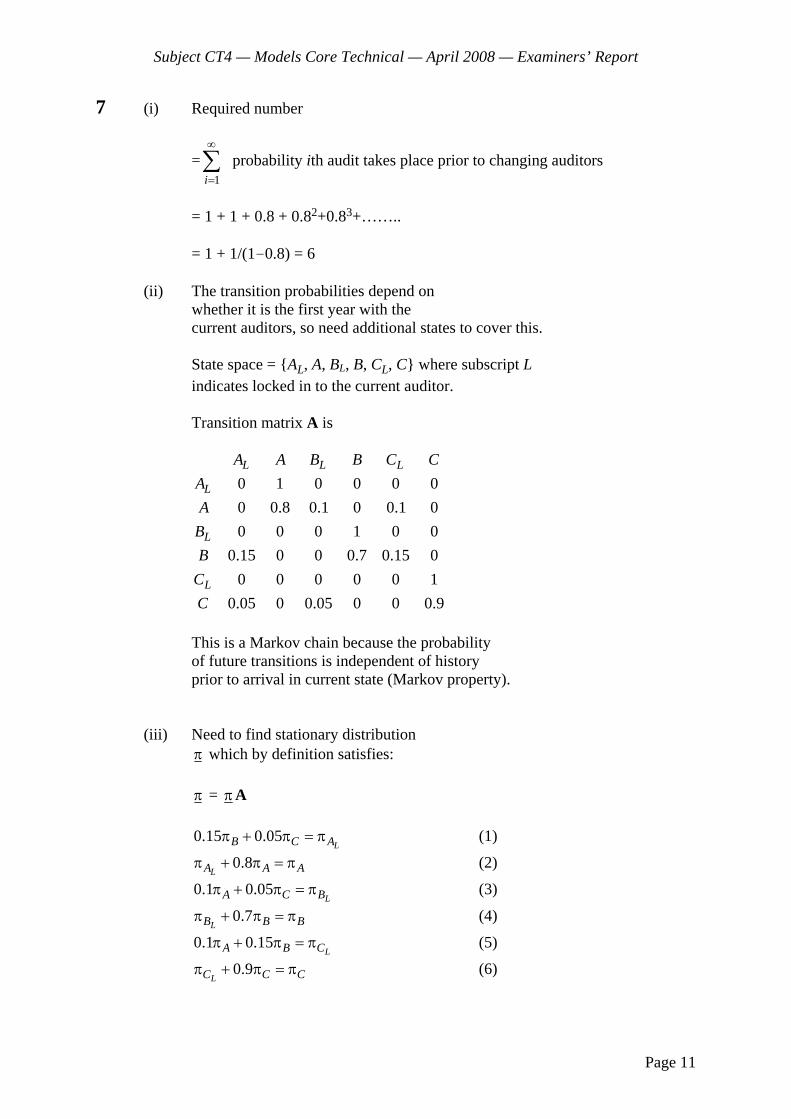
Subject CT4 — Models Core Technical — April 2008 — Examiners’ Report
Page 11
7 (i) Required number
=1i
∞
=∑ probability ith audit takes place prior to changing auditors
= 1 + 1 + 0.8 + 0.82+0.83+…….. = 1 + 1/(1-0.8) = 6
(ii) The transition probabilities depend on whether it is the first year with the current auditors, so need additional states to cover this. State space = {AL, A, BL, B, CL, C} where subscript L indicates locked in to the current auditor. Transition matrix A is
0 1 0 0 0 00 0.8 0.1 0 0.1 00 0 0 1 0 0
0.15 0 0 0.7 0.15 00 0 0 0 0 1
0.05 0 0.05 0 0 0.9
L L L
L
L
L
A A B B C CAA
BB
CC
This is a Markov chain because the probability of future transitions is independent of history prior to arrival in current state (Markov property). (iii) Need to find stationary distribution π which by definition satisfies: π = πA 0.15 0.05
LB C Aπ + π = π (1)
0.8LA A Aπ + π = π (2)
0.1 0.05LA C Bπ + π = π (3)
0.7LB B Bπ + π = π (4)
0.1 0.15LA B Cπ + π = π (5)
0.9LC C Cπ + π = π (6)
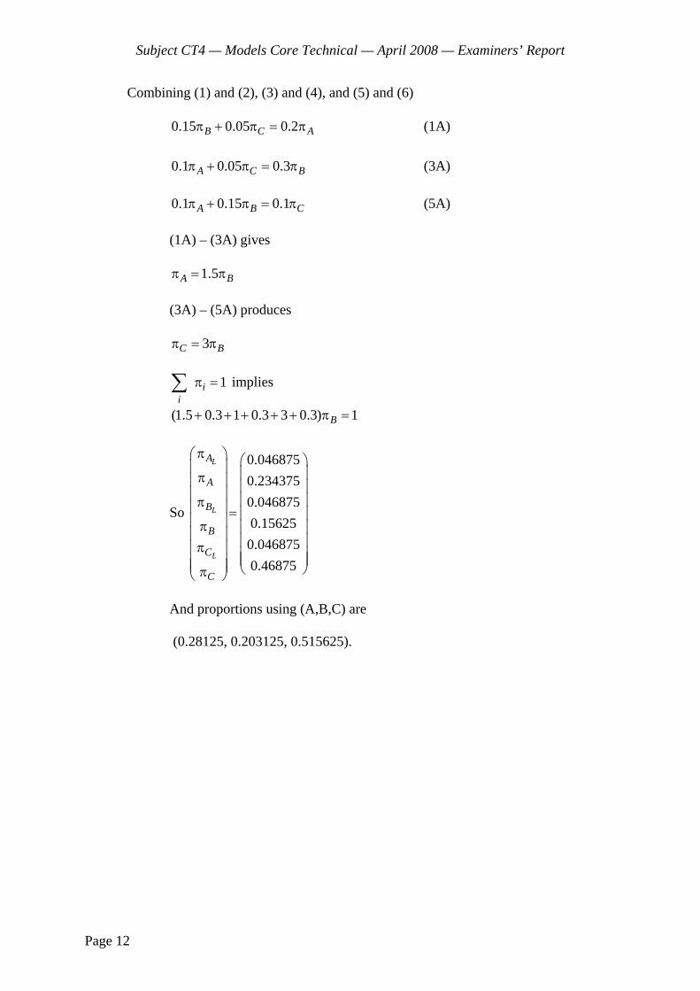
Subject CT4 — Models Core Technical — April 2008 — Examiners’ Report
Page 12
Combining (1) and (2), (3) and (4), and (5) and (6) 0.15 0.05 0.2B C Aπ + π = π (1A) 0.1 0.05 0.3A C Bπ + π = π (3A) 0.1 0.15 0.1A B Cπ + π = π (5A) (1A) – (3A) gives 1.5A Bπ = π (3A) – (5A) produces 3C Bπ = π 1i
iπ =∑ implies
(1.5 0.3 1 0.3 3 0.3) 1B+ + + + + π =
So
0.0468750.2343750.0468750.156250.0468750.46875
L
L
L
A
A
B
B
C
C
π⎛ ⎞ ⎛ ⎞⎜ ⎟ ⎜ ⎟π⎜ ⎟ ⎜ ⎟⎜ ⎟ ⎜ ⎟π⎜ ⎟ = ⎜ ⎟⎜ ⎟π ⎜ ⎟⎜ ⎟ ⎜ ⎟π⎜ ⎟ ⎜ ⎟⎜ ⎟⎜ ⎟⎜ ⎟ ⎝ ⎠π⎝ ⎠
And proportions using (A,B,C) are (0.28125, 0.203125, 0.515625).
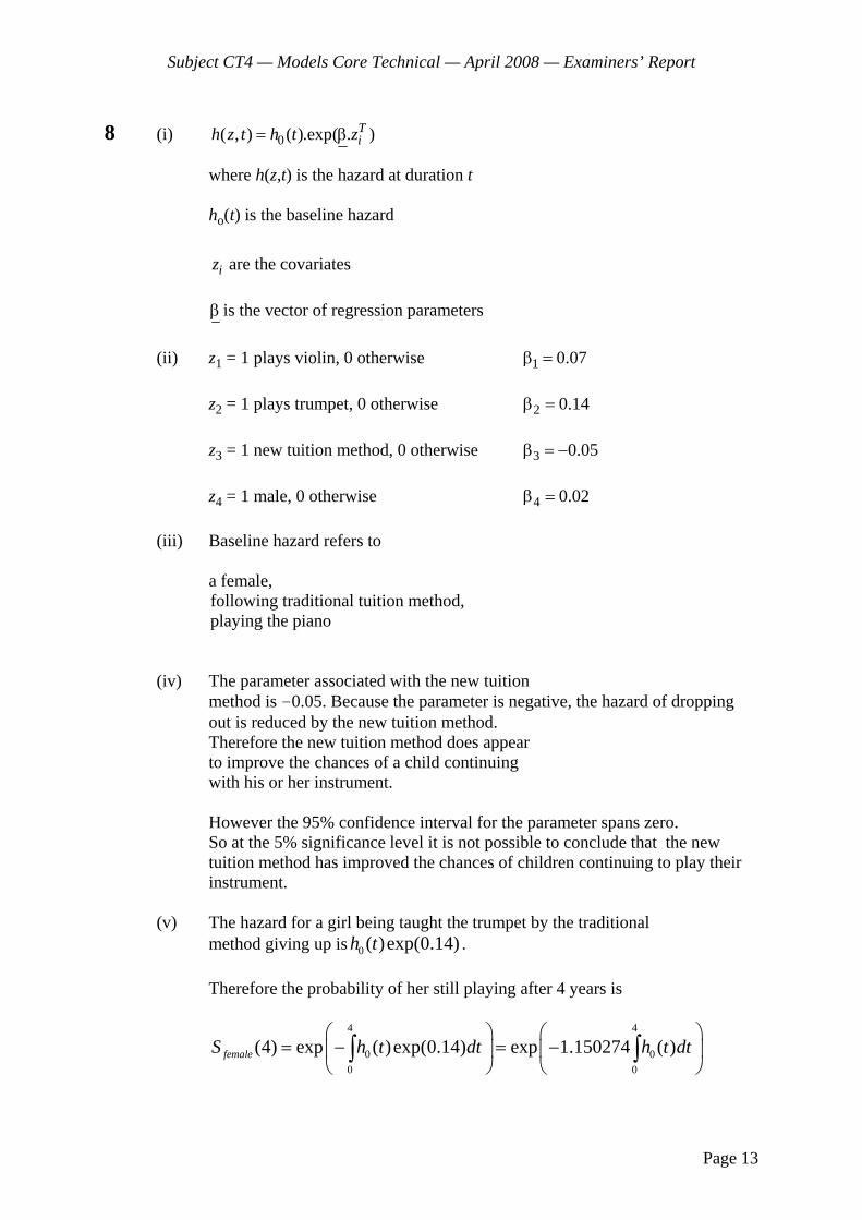
Subject CT4 — Models Core Technical — April 2008 — Examiners’ Report
Page 13
8 (i) 0( , ) ( ).exp( . )Tih z t h t z= β
where h(z,t) is the hazard at duration t ho(t) is the baseline hazard iz are the covariates β is the vector of regression parameters (ii) z1 = 1 plays violin, 0 otherwise 1 0.07β = z2 = 1 plays trumpet, 0 otherwise 2 0.14β = z3 = 1 new tuition method, 0 otherwise 3 0.05β = − z4 = 1 male, 0 otherwise 4 0.02β = (iii) Baseline hazard refers to a female, following traditional tuition method, playing the piano
(iv) The parameter associated with the new tuition
method is -0.05. Because the parameter is negative, the hazard of dropping out is reduced by the new tuition method.
Therefore the new tuition method does appear to improve the chances of a child continuing with his or her instrument. However the 95% confidence interval for the parameter spans zero.
So at the 5% significance level it is not possible to conclude that the new tuition method has improved the chances of children continuing to play their instrument.
(v) The hazard for a girl being taught the trumpet by the traditional method giving up is 0 ( )exp(0.14)h t . Therefore the probability of her still playing after 4 years is
4 4
0 00 0
(4) exp ( )exp(0.14) exp 1.150274 ( )femaleS h t dt h t dt⎛ ⎞ ⎛ ⎞
= − = −⎜ ⎟ ⎜ ⎟⎝ ⎠ ⎝ ⎠∫ ∫
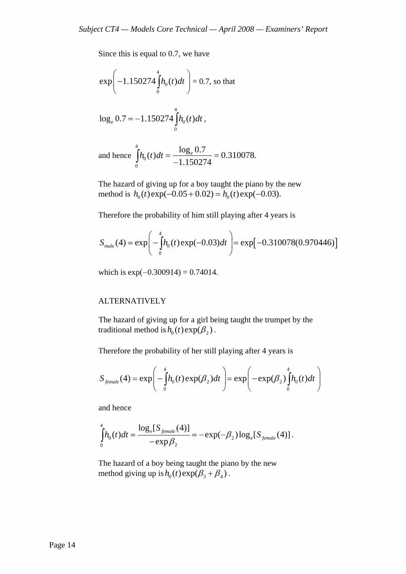
Subject CT4 — Models Core Technical — April 2008 — Examiners’ Report
Page 14
Since this is equal to 0.7, we have
4
00
exp 1.150274 ( )h t dt⎛ ⎞−⎜ ⎟⎝ ⎠
∫ = 0.7, so that
4
00
log 0.7 1.150274 ( )e h t dt= − ∫ ,
and hence 4
00
log 0.7( ) 0.310078.1.150274
eh t dt = =−∫
The hazard of giving up for a boy taught the piano by the new method is 0 0( )exp( 0.05 0.02) ( )exp( 0.03).h t h t− + = − Therefore the probability of him still playing after 4 years is
[ ]4
00
(4) exp ( )exp( 0.03) exp 0.310078(0.970446)maleS h t dt⎛ ⎞
= − − = −⎜ ⎟⎝ ⎠∫
which is exp(-0.300914) = 0.74014. ALTERNATIVELY The hazard of giving up for a girl being taught the trumpet by the
traditional method is 0 2( )exp( )h t β . Therefore the probability of her still playing after 4 years is
4 4
0 2 2 00 0
(4) exp ( )exp( ) exp exp( ) ( )femaleS h t dt h t dtβ β⎛ ⎞ ⎛ ⎞
= − = −⎜ ⎟ ⎜ ⎟⎝ ⎠ ⎝ ⎠∫ ∫
and hence
4
0 220
log [ (4)]( ) exp( ) log [ (4)]
expe female
e female
Sh t dt Sβ
β= = − −
−∫ .
The hazard of a boy being taught the piano by the new method giving up is 0 3 4( )exp( )h t β β+ .
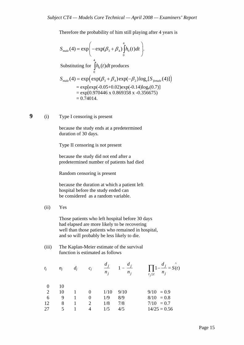
Subject CT4 — Models Core Technical — April 2008 — Examiners’ Report
Page 15
Therefore the probability of him still playing after 4 years is
4
3 4 00
(4) exp exp( ) ( )maleS h t dtβ β⎛ ⎞
= − +⎜ ⎟⎝ ⎠
∫ .
Substituting for 4
00
( )h t dt∫ produces
( )3 4 2(4) exp exp( )exp( ) log [ (4)]male e femaleS Sβ β β= + −
= exp[exp(-0.05+0.02)exp(-0.14)loge(0.7)] = exp[0.970446 x 0.869358 x -0.356675) = 0.74014. 9 (i) Type I censoring is present because the study ends at a predetermined duration of 30 days. Type II censoring is not present because the study did not end after a predetermined number of patients had died Random censoring is present because the duration at which a patient left hospital before the study ended can be considered as a random variable. (ii) Yes Those patients who left hospital before 30 days had elapsed are more likely to be recovering well than those patients who remained in hospital, and so will probably be less likely to die. (iii) The Kaplan-Meier estimate of the survival function is estimated as follows
tj nj dj cj j
j
dn
1 - j
j
dn
1j
j
jt t
dn≤
−∏ =^( )S t
0 10 2 10 1 0 1/10 9/10 9/10 = 0.9 6 9 1 0 1/9 8/9 8/10 = 0.8 12 8 1 2 1/8 7/8 7/10 = 0.7 27 5 1 4 1/5 4/5 14/25 = 0.56
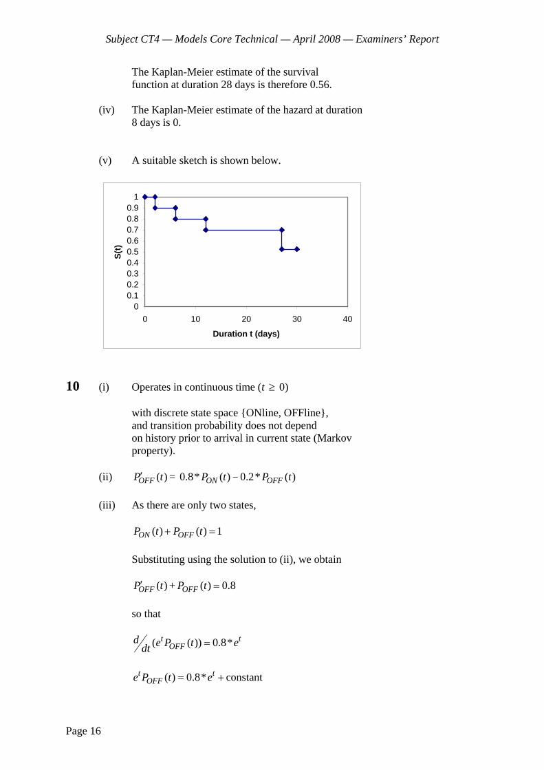
Subject CT4 — Models Core Technical — April 2008 — Examiners’ Report
Page 16
The Kaplan-Meier estimate of the survival function at duration 28 days is therefore 0.56. (iv) The Kaplan-Meier estimate of the hazard at duration 8 days is 0. (v) A suitable sketch is shown below.
00.10.20.30.40.50.60.70.80.9
1
0 10 20 30 40
Duration t (days)
S(t)
10 (i) Operates in continuous time (t ≥ 0) with discrete state space {ONline, OFFline}, and transition probability does not depend on history prior to arrival in current state (Markov property). (ii) ( )OFFP t′ = 0.8* ( )ONP t - 0.2* ( )OFFP t (iii) As there are only two states, ( ) ( ) 1ON OFFP t P t+ = Substituting using the solution to (ii), we obtain ( )OFFP t′ + ( ) 0.8OFFP t = so that ( ( )) 0.8*t t
OFFd e P t edt =
( ) 0.8* constantt t
OFFe P t e= +
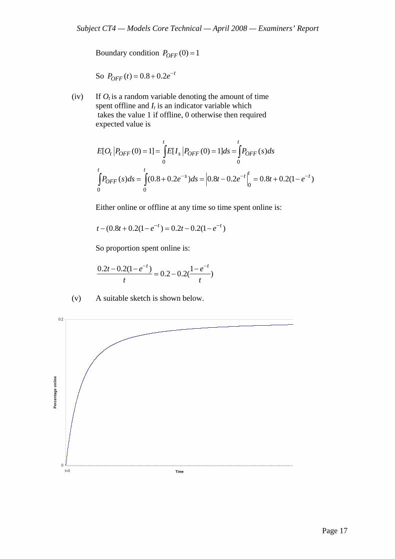
Subject CT4 — Models Core Technical — April 2008 — Examiners’ Report
Page 17
Boundary condition (0) 1OFFP = So ( ) 0.8 0.2 t
OFFP t e−= + (iv) If Ot is a random variable denoting the amount of time spent offline and It is an indicator variable which takes the value 1 if offline, 0 otherwise then required expected value is
0 0
[ (0) 1] [ (0) 1] ( )t t
t OFF s OFF OFFE O P E I P ds P s ds= = = =∫ ∫
0
0 0
( ) (0.8 0.2 ) 0.8 0.2 0.8 0.2(1 )t t ts t t
OFFP s ds e ds t e t e− − −= + = − = + −∫ ∫
Either online or offline at any time so time spent online is: (0.8 0.2(1 ) 0.2 0.2(1 )t tt t e t e− −− + − = − − So proportion spent online is:
0.2 0.2(1 ) 10.2 0.2( )t tt e e
t t
− −− − −= −
(v) A suitable sketch is shown below.
0
0.2
Time
Perc
enta
ge o
nlin
e
t=0
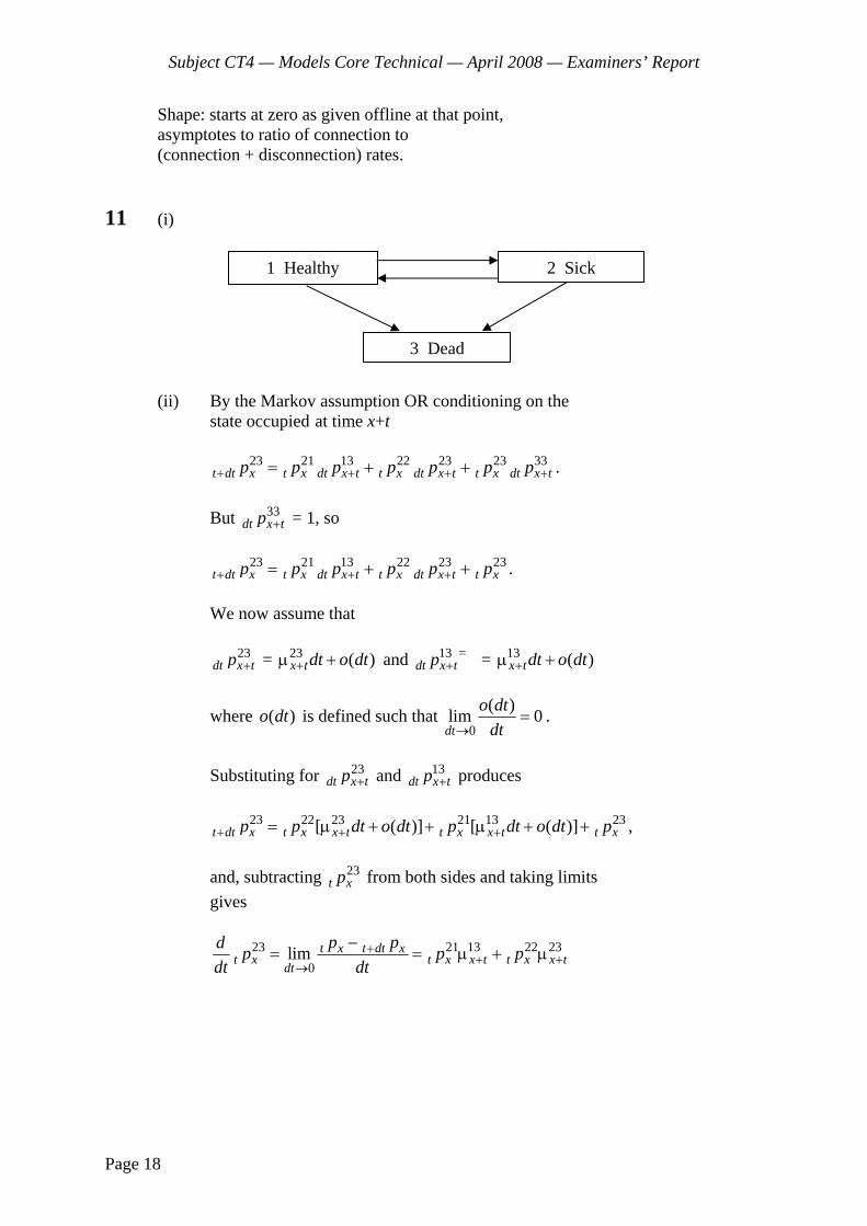
Subject CT4 — Models Core Technical — April 2008 — Examiners’ Report
Page 18
Shape: starts at zero as given offline at that point, asymptotes to ratio of connection to (connection + disconnection) rates. 11 (i) (ii) By the Markov assumption OR conditioning on the state occupied at time x+t 23 21 13 22 23 23 33
t dt x t x dt x t t x dt x t t x dt x tp p p p p p p+ + + += + + . But 33
dt x tp + = 1, so 23 21 13 22 23 23
t dt x t x dt x t t x dt x t t xp p p p p p+ + += + + . We now assume that 23
dt x tp + = 23 ( )x tdt o dt+μ + and 13 = dt x tp + = 13 ( )x tdt o dt+μ +
where ( )o dt is defined such that 0
( )lim 0dt
o dtdt→
= .
Substituting for 23
dt x tp + and 13dt x tp + produces
23 22 23 21 13 23[ ( )] [ ( )]t dt x t x x t t x x t t xp p dt o dt p dt o dt p+ + += μ + + μ + + , and, subtracting 23
t xp from both sides and taking limits gives
23 21 13 22 230
lim t x t dt xt x t x x t t x x tdt
p pd p p pdt dt
++ +
→
−= = μ + μ
1 Healthy 2 Sick
3 Dead
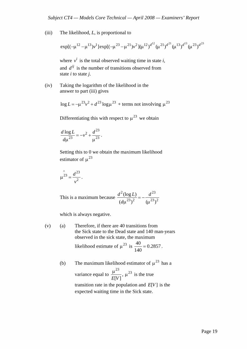
Subject CT4 — Models Core Technical — April 2008 — Examiners’ Report
Page 19
(iii) The likelihood, L, is proportional to
12 21 13 2312 13 1 23 21 2 12 21 13 23exp[( ) ]exp[( ) ]( ) ( ) ( ) ( )d d d dv v−μ −μ −μ −μ μ μ μ μ
where iv is the total observed waiting time in state i, and ijd is the number of transitions observed from state i to state j. (iv) Taking the logarithm of the likelihood in the answer to part (iii) gives 23 2 23 23log logL v d= −μ + μ + terms not involving 23μ Differentiating this with respect to 23μ we obtain
23
223 23
logd L dvd
= − +μ μ
.
Setting this to 0 we obtain the maximum likelihood estimator of 23μ
^ 2323
2dv
μ = .
This is a maximum because 2 23
23 2 23 2(log )
( ) ( )d L d
d= −
μ μ
which is always negative. (v) (a) Therefore, if there are 40 transitions from the Sick state to the Dead state and 140 man-years observed in the sick state, the maximum
likelihood estimate of 23μ is 40 0.2857140
= .
(b) The maximum likelihood estimator of 23μ has a
variance equal to 23
[ ]E Vμ , 23μ is the true
transition rate in the population and [ ]E V is the expected waiting time in the Sick state.
Subject CT4 — Models Core Technical — April 2008 — Examiners’ Report
Page 20
Approximating 23μ by ^23μ and [ ]E V by 2v we
estimate for the variance as 0.2857 0.00204140
= .
A 95 per cent confidence interval around our estimate of 23μ is therefore 0.2857 1.96 0.00204± which is 0.2857 0.0885± or (0.1972, 0.3742).
END OF EXAMINERS’ REPORT

Faculty of Actuaries Institute of Actuaries
EXAMINATION
17 September 2008 (am)
Subject CT4 — Models Core Technical
Time allowed: Three hours
INSTRUCTIONS TO THE CANDIDATE
1. Enter all the candidate and examination details as requested on the front of your answer booklet.
2. You must not start writing your answers in the booklet until instructed to do so by the
supervisor. 3. Mark allocations are shown in brackets. 4. Attempt all 12 questions, beginning your answer to each question on a separate sheet. 5. Candidates should show calculations where this is appropriate.
Graph paper is not required for this paper.
AT THE END OF THE EXAMINATION
Hand in BOTH your answer booklet, with any additional sheets firmly attached, and this question paper.
In addition to this paper you should have available the 2002 edition of the Formulae and Tables and your own electronic calculator from the approved list.
© Faculty of Actuaries CT4 S2008 © Institute of Actuaries

CT4 S2008—2
1 You work for a consultancy which has created an actuarial model and is now preparing documentation for the client.
List the key items you would include in the documentation on the model. [4] 2 The classification of stochastic models according to:
• discrete or continuous time variable • discrete or continuous state space
gives rise to a four-way classification. Give four examples, one of each type, of stochastic models which may be used to
model observed processes, and suggest a practical problem to which each model may be applied. [4]
3 Compare the advantages and disadvantages of the Binomial and the multiple-state
models in the following situations:
(a) analysing human mortality without distinguishing between causes of death (b) analysing human mortality when distinguishing between causes of death
[5] 4 In the village of Selborne in southern England in the year 1637 the number of babies
born each month was as follows January 2 July 5 February 1 August 1 March 1 September 0 April 2 October 2 May 1 November 0 June 2 December 3 Data show that over the 20 years before 1637 there was an average of 1.5 births per month. You may assume that births in the village historically follow a Poisson process. An historian has suggested that the large number of births in July 1637 is unusual. (i) Carry out a test of the historian’s suggestion, stating your conclusion. [4] (ii) Comment on the assumption that births follow a Poisson process. [1]
[Total 5]

CT4 S2008—3 PLEASE TURN OVER
5 An investigation into the mortality experience of a sample of the male student population of a large university has been carried out. The university authorities wish to know whether the mortality of male students at the university is the same as that of males in the country as a whole. They have drawn up the following table.
Age x Number of deaths Expected number of deaths assuming national mortality 18 13 10 19 15 12 20 14 14 21 20 12 22 12 8 23 8 5 Carry out an overall test of the university authorities’ hypothesis, stating your
conclusion. [5]
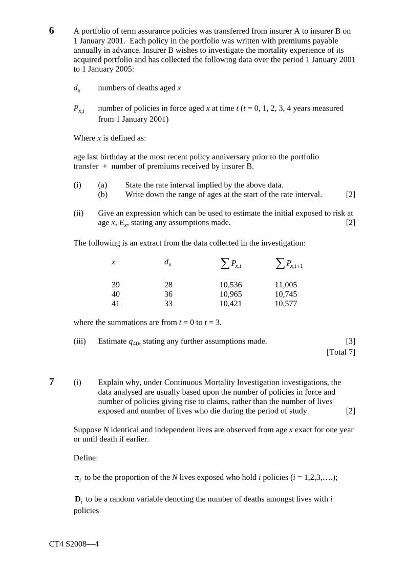
CT4 S2008—4
6 A portfolio of term assurance policies was transferred from insurer A to insurer B on 1 January 2001. Each policy in the portfolio was written with premiums payable annually in advance. Insurer B wishes to investigate the mortality experience of its acquired portfolio and has collected the following data over the period 1 January 2001 to 1 January 2005:
dx numbers of deaths aged x Px,t number of policies in force aged x at time t (t = 0, 1, 2, 3, 4 years measured
from 1 January 2001) Where x is defined as: age last birthday at the most recent policy anniversary prior to the portfolio transfer + number of premiums received by insurer B. (i) (a) State the rate interval implied by the above data. (b) Write down the range of ages at the start of the rate interval. [2] (ii) Give an expression which can be used to estimate the initial exposed to risk at
age x, Ex, stating any assumptions made. [2] The following is an extract from the data collected in the investigation:
x dx ,x tP∑
, 1x tP +∑
39 28 10,536 11,005 40 36 10,965 10,745 41 33 10,421 10,577
where the summations are from t = 0 to t = 3. (iii) Estimate q40, stating any further assumptions made. [3] [Total 7] 7 (i) Explain why, under Continuous Mortality Investigation investigations, the
data analysed are usually based upon the number of policies in force and number of policies giving rise to claims, rather than the number of lives exposed and number of lives who die during the period of study. [2]
Suppose N identical and independent lives are observed from age x exact for one year
or until death if earlier. Define: iπ to be the proportion of the N lives exposed who hold i policies (i = 1,2,3,….); iD to be a random variable denoting the number of deaths amongst lives with i
policies

CT4 S2008—5 PLEASE TURN OVER
iC to be a random variable denoting the number of claims arising from lives with i policies.
(ii) Derive an expression for the ratio of the variance of the number of claims
arising compared with that if each policy covered an independent life. [4] (iii) Explain how the expression derived in (ii) could be used in practice. [2] [Total 8] 8 A No-Claims Discount system operated by a motor insurer has the following four
levels: Level 1: 0% discount Level 2: 25% discount Level 3: 40% discount Level 4: 60% discount The rules for moving between these levels are as follows:
• Following a year with no claims, move to the next higher level, or remain at level 4.
• Following a year with one claim, move to the next lower level, or remain at
level 1.
• Following a year with two or more claims, move down two levels, or move to level 1 (from level 2) or remain at level 1.
For a given policyholder in a given year the probability of no claims is 0.85 and the
probability of making one claim is 0.12. (i) Write down the transition matrix of this No-Claims Discount process. [1] (ii) Calculate the probability that a policyholder who is currently at level 2 will be
at level 2 after: (a) one year. (b) two years. [3] (iii) Calculate the long-run probability that a policyholder is in discount level 2. [5] [Total 9]
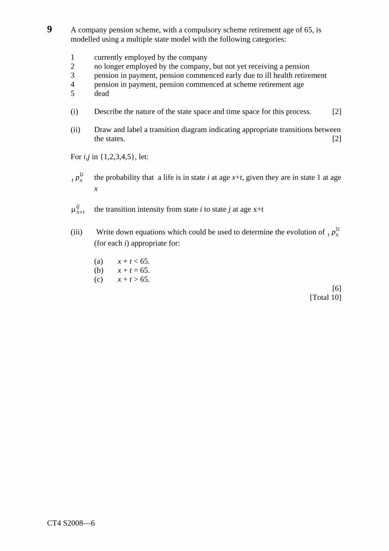
CT4 S2008—6
9 A company pension scheme, with a compulsory scheme retirement age of 65, is modelled using a multiple state model with the following categories:
1 currently employed by the company 2 no longer employed by the company, but not yet receiving a pension 3 pension in payment, pension commenced early due to ill health retirement 4 pension in payment, pension commenced at scheme retirement age 5 dead
(i) Describe the nature of the state space and time space for this process. [2] (ii) Draw and label a transition diagram indicating appropriate transitions between
the states. [2] For i,j in {1,2,3,4,5}, let: 1i
t xp the probability that a life is in state i at age x+t, given they are in state 1 at age x
ij
x t+μ the transition intensity from state i to state j at age x+t (iii) Write down equations which could be used to determine the evolution of 1i
t xp (for each i) appropriate for:
(a) x + t < 65. (b) x + t = 65. (c) x + t > 65. [6] [Total 10]
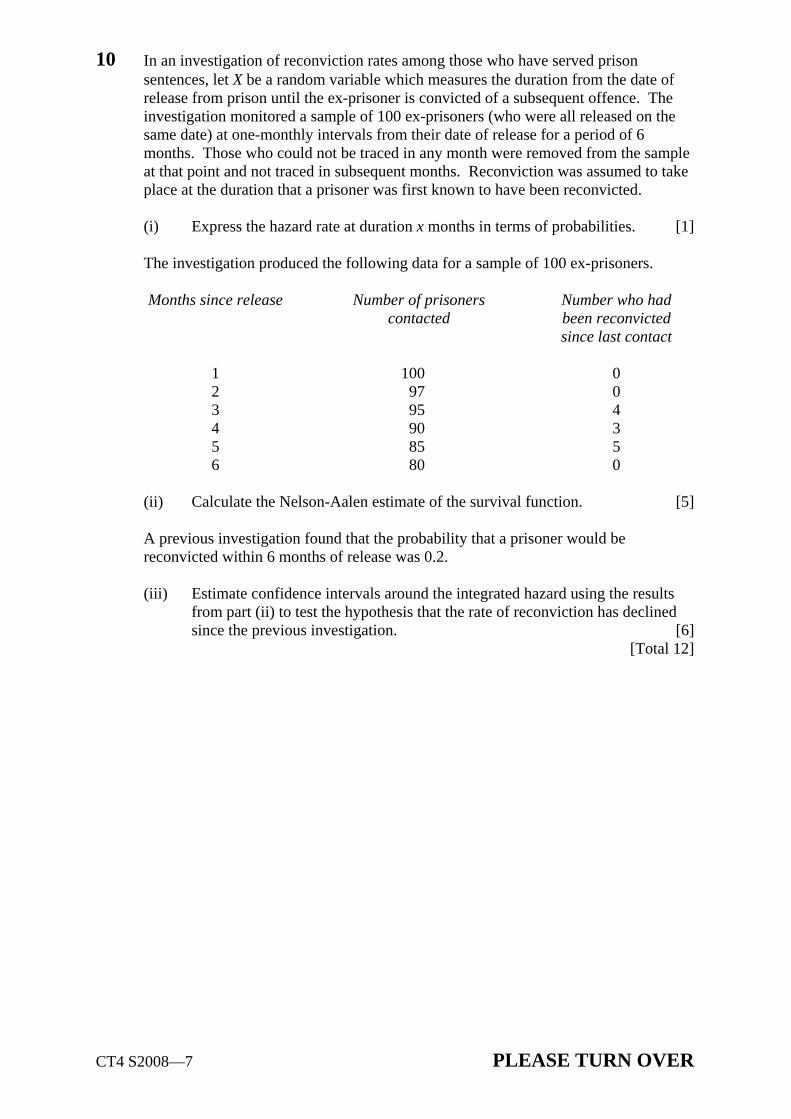
CT4 S2008—7 PLEASE TURN OVER
10 In an investigation of reconviction rates among those who have served prison sentences, let X be a random variable which measures the duration from the date of release from prison until the ex-prisoner is convicted of a subsequent offence. The investigation monitored a sample of 100 ex-prisoners (who were all released on the same date) at one-monthly intervals from their date of release for a period of 6 months. Those who could not be traced in any month were removed from the sample at that point and not traced in subsequent months. Reconviction was assumed to take place at the duration that a prisoner was first known to have been reconvicted.
(i) Express the hazard rate at duration x months in terms of probabilities. [1] The investigation produced the following data for a sample of 100 ex-prisoners. Months since release Number of prisoners Number who had contacted been reconvicted since last contact 1 100 0 2 97 0 3 95 4 4 90 3 5 85 5 6 80 0 (ii) Calculate the Nelson-Aalen estimate of the survival function. [5] A previous investigation found that the probability that a prisoner would be
reconvicted within 6 months of release was 0.2. (iii) Estimate confidence intervals around the integrated hazard using the results
from part (ii) to test the hypothesis that the rate of reconviction has declined since the previous investigation. [6]
[Total 12]
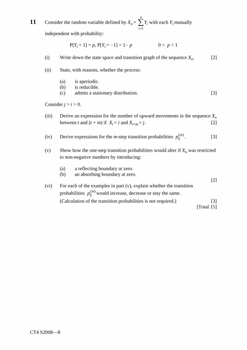
CT4 S2008—8
11 Consider the random variable defined by Xn = 1
n
ii
Y=∑ with each Yi mutually
independent with probability:
P[Yi = 1] = p, P[Yi = -1] = 1- p 0 < p < 1 (i) Write down the state space and transition graph of the sequence Xn. [2] (ii) State, with reasons, whether the process: (a) is aperiodic. (b) is reducible. (c) admits a stationary distribution. [3] Consider j > i > 0. (iii) Derive an expression for the number of upward movements in the sequence Xn
between t and (t + m) if Xt = i and Xt+m = j. [2] (iv) Derive expressions for the m-step transition probabilities ( )m
ijp . [3] (v) Show how the one-step transition probabilities would alter if Xn was restricted
to non-negative numbers by introducing: (a) a reflecting boundary at zero. (b) an absorbing boundary at zero. [2] (vi) For each of the examples in part (v), explain whether the transition
probabilities ( )mijp would increase, decrease or stay the same.
(Calculation of the transition probabilities is not required.) [3] [Total 15]
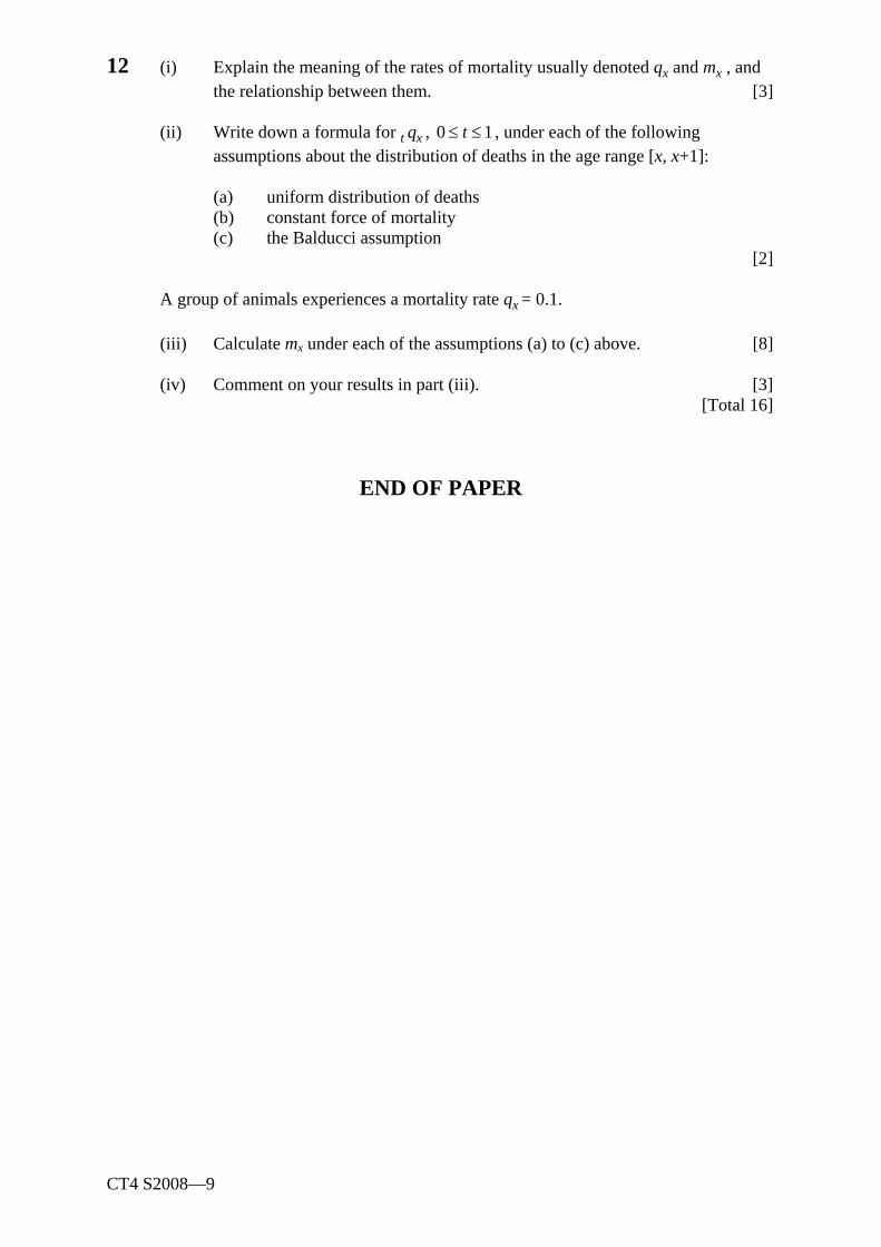
CT4 S2008—9
12 (i) Explain the meaning of the rates of mortality usually denoted qx and mx , and the relationship between them. [3]
(ii) Write down a formula for t qx , 0 1t≤ ≤ , under each of the following
assumptions about the distribution of deaths in the age range [x, x+1]: (a) uniform distribution of deaths (b) constant force of mortality (c) the Balducci assumption
[2] A group of animals experiences a mortality rate qx = 0.1. (iii) Calculate mx under each of the assumptions (a) to (c) above. [8] (iv) Comment on your results in part (iii). [3] [Total 16]
END OF PAPER

Faculty of Actuaries Institute of Actuaries
Subject CT4 — Models Core Technical
EXAMINERS’ REPORT
September 2008
Introduction The attached subject report has been written by the Principal Examiner with the aim of helping candidates. The questions and comments are based around Core Reading as the interpretation of the syllabus to which the examiners are working. They have however given credit for any alternative approach or interpretation which they consider to be reasonable. R D Muckart Chairman of the Board of Examiners November 2008
© Faculty of Actuaries © Institute of Actuaries
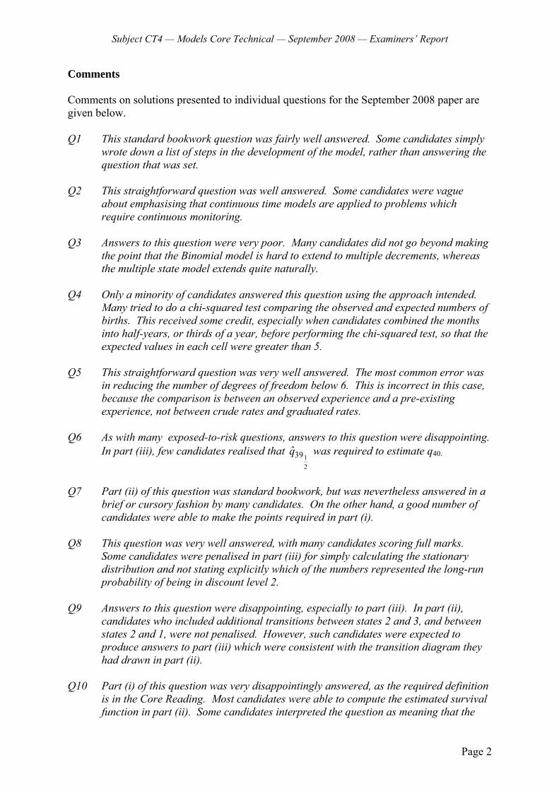
Subject CT4 — Models Core Technical — September 2008 — Examiners’ Report
Page 2
Comments Comments on solutions presented to individual questions for the September 2008 paper are given below. Q1 This standard bookwork question was fairly well answered. Some candidates simply
wrote down a list of steps in the development of the model, rather than answering the question that was set.
Q2 This straightforward question was well answered. Some candidates were vague
about emphasising that continuous time models are applied to problems which require continuous monitoring.
Q3 Answers to this question were very poor. Many candidates did not go beyond making
the point that the Binomial model is hard to extend to multiple decrements, whereas the multiple state model extends quite naturally.
Q4 Only a minority of candidates answered this question using the approach intended.
Many tried to do a chi-squared test comparing the observed and expected numbers of births. This received some credit, especially when candidates combined the months into half-years, or thirds of a year, before performing the chi-squared test, so that the expected values in each cell were greater than 5.
Q5 This straightforward question was very well answered. The most common error was
in reducing the number of degrees of freedom below 6. This is incorrect in this case, because the comparison is between an observed experience and a pre-existing experience, not between crude rates and graduated rates.
Q6 As with many exposed-to-risk questions, answers to this question were disappointing.
In part (iii), few candidates realised that 12
39q was required to estimate q40.
Q7 Part (ii) of this question was standard bookwork, but was nevertheless answered in a
brief or cursory fashion by many candidates. On the other hand, a good number of candidates were able to make the points required in part (i).
Q8 This question was very well answered, with many candidates scoring full marks.
Some candidates were penalised in part (iii) for simply calculating the stationary distribution and not stating explicitly which of the numbers represented the long-run probability of being in discount level 2.
Q9 Answers to this question were disappointing, especially to part (iii). In part (ii),
candidates who included additional transitions between states 2 and 3, and between states 2 and 1, were not penalised. However, such candidates were expected to produce answers to part (iii) which were consistent with the transition diagram they had drawn in part (ii).
Q10 Part (i) of this question was very disappointingly answered, as the required definition
is in the Core Reading. Most candidates were able to compute the estimated survival function in part (ii). Some candidates interpreted the question as meaning that the
Subject CT4 — Models Core Technical — September 2008 — Examiners’ Report
Page 3
numbers contacted at any duration include those reconvicted prior to that duration, so that those reconvicted must be subtracted from those contacted to obtain the relevant nj. These candidates were given credit for part (ii). In part (iii) many candidates correctly calculated the variance of the integrated hazard but then incorrectly used this variance to compute a confidence interval around the survival function, rather than first computing the confidence interval around the integrated hazard and then using the formula S(x) = exp(−Λx) to convert this into a confidence interval around S(6).
Q11 Answers to this question were disappointing. Many candidates were able to answer
parts (i) and (ii) reasonably well, but made little or no attempt at the remaining sections.
Q12 Answers to this question varied widely, but overall were disappointing. There was a
large variation by centre, with average scores for some centres being several marks higher than for other centres. Perhaps this is the result of different training and education materials being used in different locations? While most candidates could
write down the formula 1
0
xx
t x
qm
p dt
=
∫ and the formulae required to answer part (ii), it
was clear from the answers to parts (iii) and (iv) that understanding of what these formulae mean was very shaky.

Subject CT4 — Models Core Technical — September 2008 — Examiners’ Report
Page 4
1 Instructions on how to run the model Tests performed to validate the output of the model. Definition of input data. Any limitations of the model identified (e.g. potential unreliability). Basis on which the form of the model chosen (e.g. deterministic or stochastic) References to any research papers or discussions with appropriate experts. Summary of model results. Name and professional qualification. Purpose or objectives of the model. Assumptions underlying the model. How the model might be adapted or extended. 2 Discrete time, discrete state space Counting process, random walk, Markov chain No claims bonus in motor insurance. Continuous time, discrete state space Counting process, Poisson process, Markov jump process Healthy-sick-dead model in sickness insurance Discrete time, continuous state space General random walk, ARIMA time series model, moving average model Share price at end of each day Continuous time, continuous state space Compound Poisson process, Brownian motion, Ito process, white noise Value of claims reaching an insurance company monitored continuously

Subject CT4 — Models Core Technical — September 2008 — Examiners’ Report
Page 5
3 (a) Both models produce consistent and unbiased estimators. The estimate of xq made using the Binomial model will have a higher variance than that made using the multiple-state model, though the difference is tiny if the forces of mortality are small. If data on exact ages at entry into and exit from observation are available, the multiple state model is simpler to apply. The Binomial model requires further assumptions (e.g. uniform distribution of deaths). The Binomial model also does not use all the information available if exact ages at entry into and exit from observation are available. However, if the forces of mortality are small, both models will give very similar results. (b) The multiple state model can simply be extended The estimators have the same form and the same statistical properties as in the classic life table. The Binomial model is hard to extend to several causes of death. Although the life table as a computational tool can be extended, the calculations are more complex and awkward than those in the multiple-state model. 4 (i) Suppose that the number of births each month, B, is the outcome of a Poisson
process with a rate λ = 1.5. The probability of obtaining b births per month
is given by the formula exp( 1.5).1.5Pr[ ]!
bB b
b−
= =
Therefore we have b Pr[ ]B b= 0 0.223 1 0.335 2 0.251 3 0.126 4 0.047 5 0.014 6+ 0.004
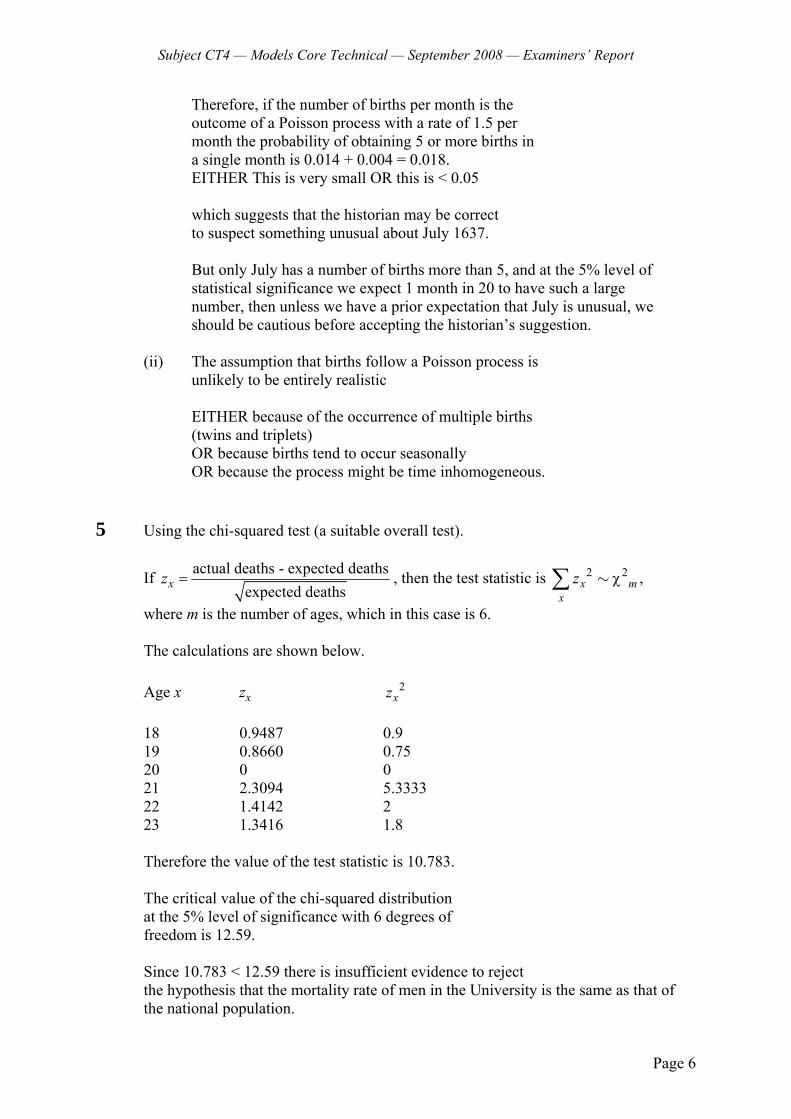
Subject CT4 — Models Core Technical — September 2008 — Examiners’ Report
Page 6
Therefore, if the number of births per month is the outcome of a Poisson process with a rate of 1.5 per month the probability of obtaining 5 or more births in a single month is 0.014 + 0.004 = 0.018. EITHER This is very small OR this is < 0.05 which suggests that the historian may be correct to suspect something unusual about July 1637. But only July has a number of births more than 5, and at the 5% level of
statistical significance we expect 1 month in 20 to have such a large number, then unless we have a prior expectation that July is unusual, we should be cautious before accepting the historian’s suggestion.
(ii) The assumption that births follow a Poisson process is unlikely to be entirely realistic
EITHER because of the occurrence of multiple births (twins and triplets) OR because births tend to occur seasonally OR because the process might be time inhomogeneous.
5 Using the chi-squared test (a suitable overall test).
If actual deaths - expected deathsexpected deathsxz = , then the test statistic is 2 2
x mx
z χ∑ ∼ ,
where m is the number of ages, which in this case is 6. The calculations are shown below. Age x zx 2
xz 18 0.9487 0.9 19 0.8660 0.75 20 0 0 21 2.3094 5.3333 22 1.4142 2 23 1.3416 1.8 Therefore the value of the test statistic is 10.783. The critical value of the chi-squared distribution at the 5% level of significance with 6 degrees of freedom is 12.59. Since 10.783 < 12.59 there is insufficient evidence to reject the hypothesis that the mortality rate of men in the University is the same as that of
the national population.
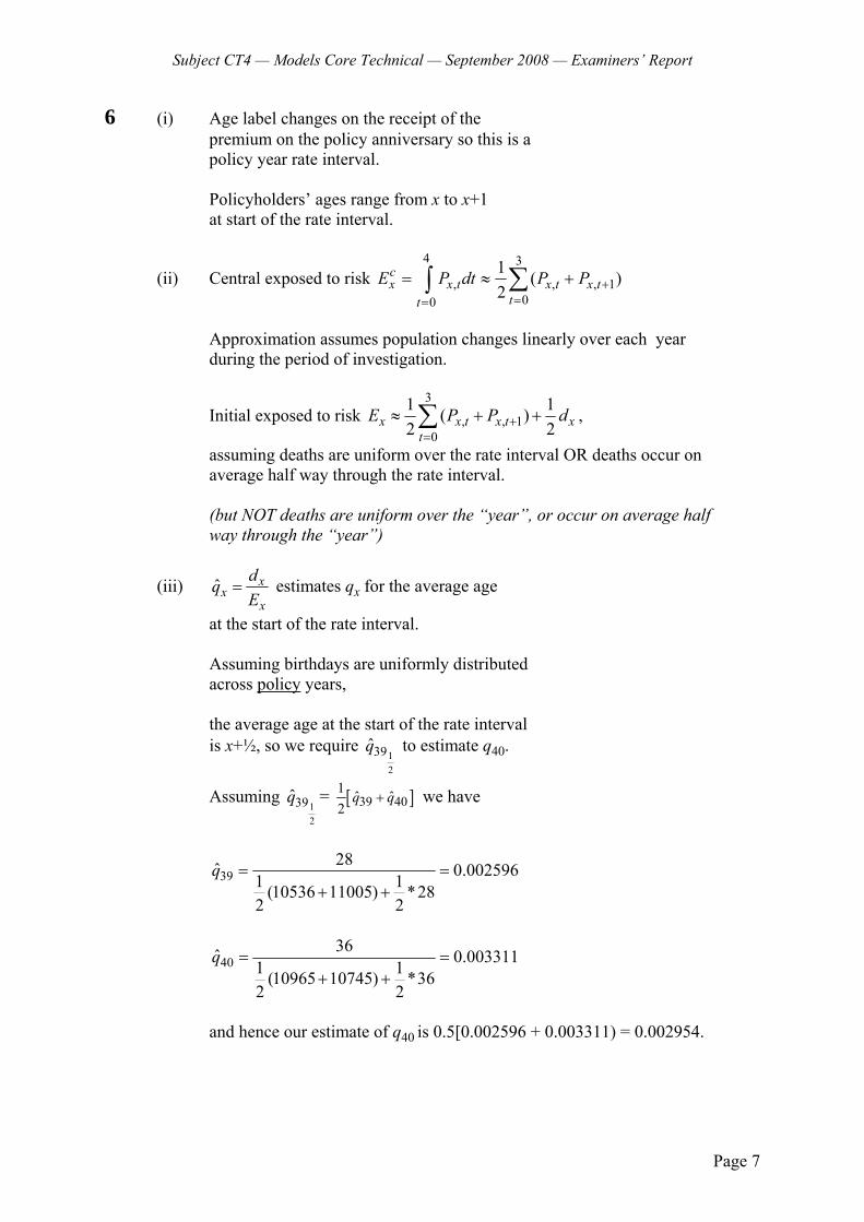
Subject CT4 — Models Core Technical — September 2008 — Examiners’ Report
Page 7
6 (i) Age label changes on the receipt of the premium on the policy anniversary so this is a policy year rate interval.
Policyholders’ ages range from x to x+1 at start of the rate interval.
(ii) Central exposed to risk 4 3
, , , 100
1 ( )2
cx x t x t x t
tt
E P dt P P +==
= ≈ +∑∫
Approximation assumes population changes linearly over each year
during the period of investigation.
Initial exposed to risk 3
, , 10
1 1( )2 2x x t x t x
tE P P d+
=
≈ + +∑ ,
assuming deaths are uniform over the rate interval OR deaths occur on average half way through the rate interval. (but NOT deaths are uniform over the “year”, or occur on average half way through the “year”)
(iii) ˆ xx
x
dqE
= estimates qx for the average age
at the start of the rate interval.
Assuming birthdays are uniformly distributed across policy years, the average age at the start of the rate interval is x+½, so we require
12
39q to estimate q40.
Assuming 12
39q = [ ]39 401 ˆ ˆ2
q q+ we have
3928ˆ 0.0025961 1(10536 11005) *28
2 2
q = =+ +
4036ˆ 0.0033111 1(10965 10745) *36
2 2
q = =+ +
and hence our estimate of q40 is 0.5[0.002596 + 0.003311) = 0.002954.
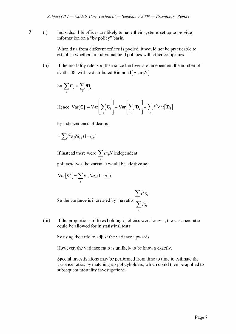
Subject CT4 — Models Core Technical — September 2008 — Examiners’ Report
Page 8
7 (i) Individual life offices are likely to have their systems set up to provide information on a “by policy” basis.
When data from different offices is pooled, it would not be practicable to establish whether an individual held policies with other companies.
(ii) If the mortality rate is qx then since the lives are independent the number of deaths iD will be distributed Binomial ( ),x iq Nπ
So i i
i ii=∑ ∑C D .
Hence Var[C] [ ]2
iVar Var Vari i i
i ii i
⎡ ⎤ ⎡ ⎤= = =⎢ ⎥ ⎢ ⎥
⎢ ⎥⎢ ⎥ ⎣ ⎦⎣ ⎦∑ ∑ ∑C D D
by independence of deaths 2 (1 )i x x
ii Nq q= π −∑
If instead there were i
ii Nπ∑ independent
policies/lives the variance would be additive so: [ ]Var (1 )i x x
ii Nq q′ = π −∑C
So the variance is increased by the ratio
2i
i
ii
i
i
π
π
∑∑
(iii) If the proportions of lives holding i policies were known, the variance ratio
could be allowed for in statistical tests by using the ratio to adjust the variance upwards. However, the variance ratio is unlikely to be known exactly. Special investigations may be performed from time to time to estimate the
variance ratios by matching up policyholders, which could then be applied to subsequent mortality investigations.
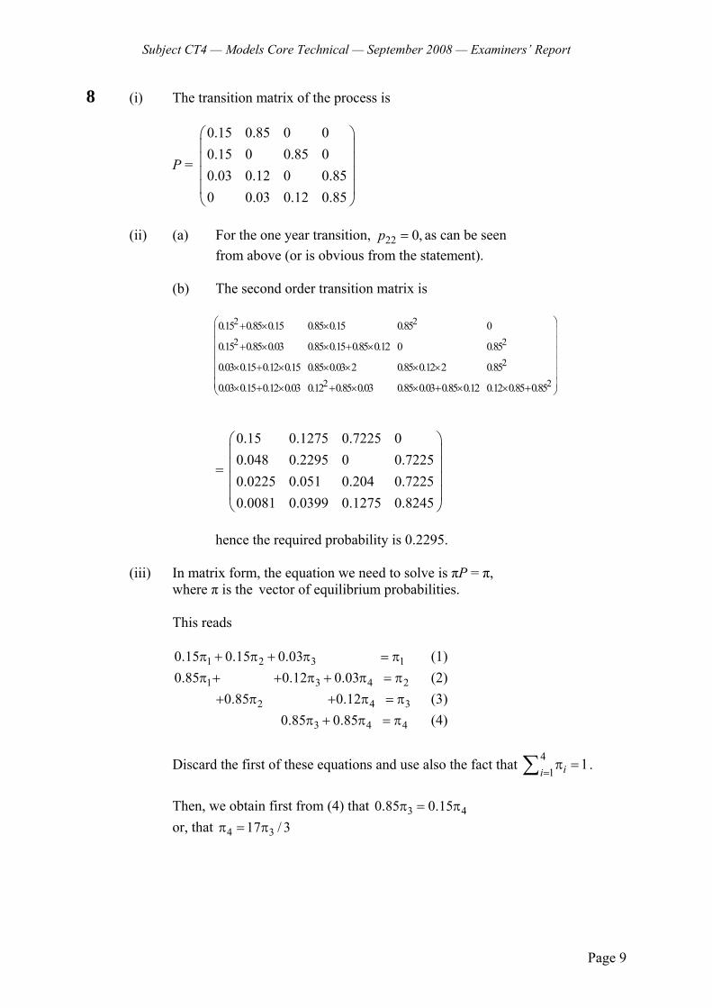
Subject CT4 — Models Core Technical — September 2008 — Examiners’ Report
Page 9
8 (i) The transition matrix of the process is
P =
0.15 0.85 0 00.15 0 0.85 00.03 0.12 0 0.850 0.03 0.12 0.85
⎛ ⎞⎜ ⎟⎜ ⎟⎜ ⎟⎜ ⎟⎝ ⎠
(ii) (a) For the one year transition, 22 0,p = as can be seen from above (or is obvious from the statement). (b) The second order transition matrix is
2 2
2 2
2
2 2
0.15 0.85 0.15 0.85 0.15 0.85 0
0.15 0.85 0.03 0.85 0.15 0.85 0.12 0 0.85
0.03 0.15 0.12 0.15 0.85 0.03 2 0.85 0.12 2 0.85
0.03 0.15 0.12 0.03 0.12 0.85 0.03 0.85 0.03 0.85 0.12 0.12 0.85 0.85
⎛ ⎞+ × ×⎜ ⎟⎜ ⎟+ × × + ×⎜ ⎟⎜ ⎟× + × × × × ×⎜ ⎟⎜ ⎟× + × + × × + × × +⎝ ⎠
=
0.15 0.1275 0.7225 00.048 0.2295 0 0.72250.0225 0.051 0.204 0.72250.0081 0.0399 0.1275 0.8245
⎛ ⎞⎜ ⎟⎜ ⎟⎜ ⎟⎜ ⎟⎝ ⎠
hence the required probability is 0.2295. (iii) In matrix form, the equation we need to solve is πP = π, where π is the vector of equilibrium probabilities. This reads 1 2 3 10.15 0.15 0.03π + π + π = π (1) 1 3 4 20.85 0.12 0.03π + + π + π = π (2) 2 4 30.85 0.12+ π + π = π (3) 3 4 40.85 0.85π + π = π (4)
Discard the first of these equations and use also the fact that 41
1ii=π =∑ .
Then, we obtain first from (4) that 3 40.85 0.15π = π or, that 4 317 / 3π = π
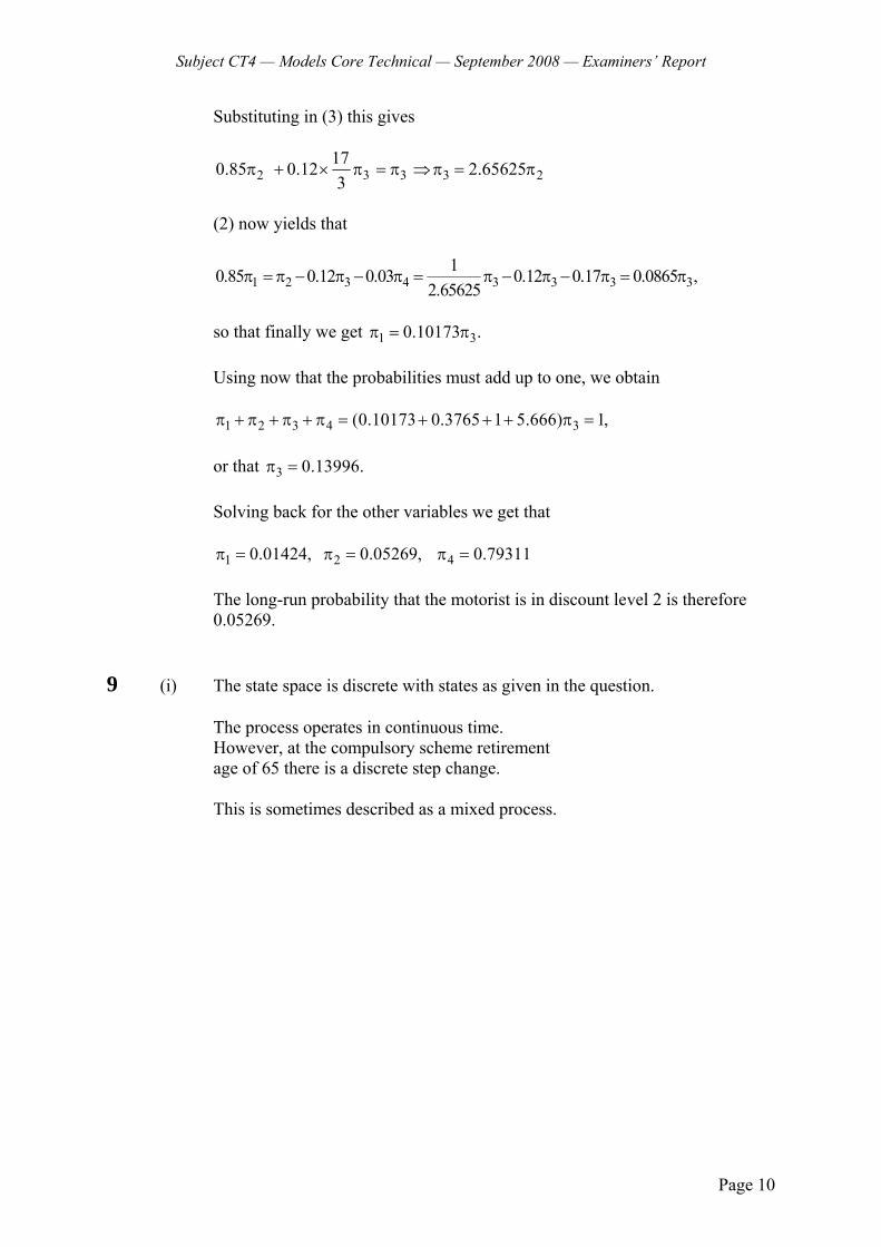
Subject CT4 — Models Core Technical — September 2008 — Examiners’ Report
Page 10
Substituting in (3) this gives
2 3 3 3 2170.85 0.12 2.656253
π + × π = π ⇒π = π
(2) now yields that
1 2 3 4 3 3 3 310.85 0.12 0.03 0.12 0.17 0.0865 ,
2.65625π = π − π − π = π − π − π = π
so that finally we get 1 30.10173 .π = π Using now that the probabilities must add up to one, we obtain 1 2 3 4 3(0.10173 0.3765 1 5.666) 1,π + π + π + π = + + + π = or that 3 0.13996.π = Solving back for the other variables we get that 1 2 40.01424, 0.05269, 0.79311π = π = π = The long-run probability that the motorist is in discount level 2 is therefore
0.05269. 9 (i) The state space is discrete with states as given in the question.
The process operates in continuous time. However, at the compulsory scheme retirement age of 65 there is a discrete step change. This is sometimes described as a mixed process.
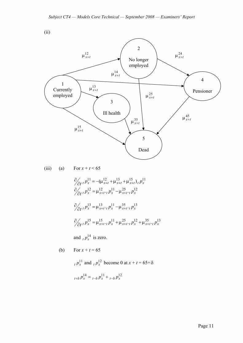
Subject CT4 — Models Core Technical — September 2008 — Examiners’ Report
Page 11
(ii)
(iii) (a) For x + t < 65
11 12 13 15 11( )t x x t x t x t t xp pt + + +
∂ = − μ +μ +μ∂
12 12 11 25 12. .t x x t t x x t t xp p pt + +∂ = μ −μ∂
13 13 11 35 13. .t x x t t x x t t xp p pt + +
∂ = μ −μ∂
15 15 11 25 12 35 13. . .t x x t t x x t t x x t t xp p p pt + + +
∂ = μ +μ +μ∂
and 14
t xp is zero. (b) For x + t = 65
11
t xp and 12t xp become 0 at x + t = 65+δ
14 11 12
t x t x t xp p p+δ −δ −δ= +
14x t+μ
12x t+μ 24
x t+μ
35x t+μ
13x t+μ
1 Currently employed
2
No longer employed
4
Pensioner
3
Ill health
5
Dead
25x t+μ
45x t+μ
15x t+μ
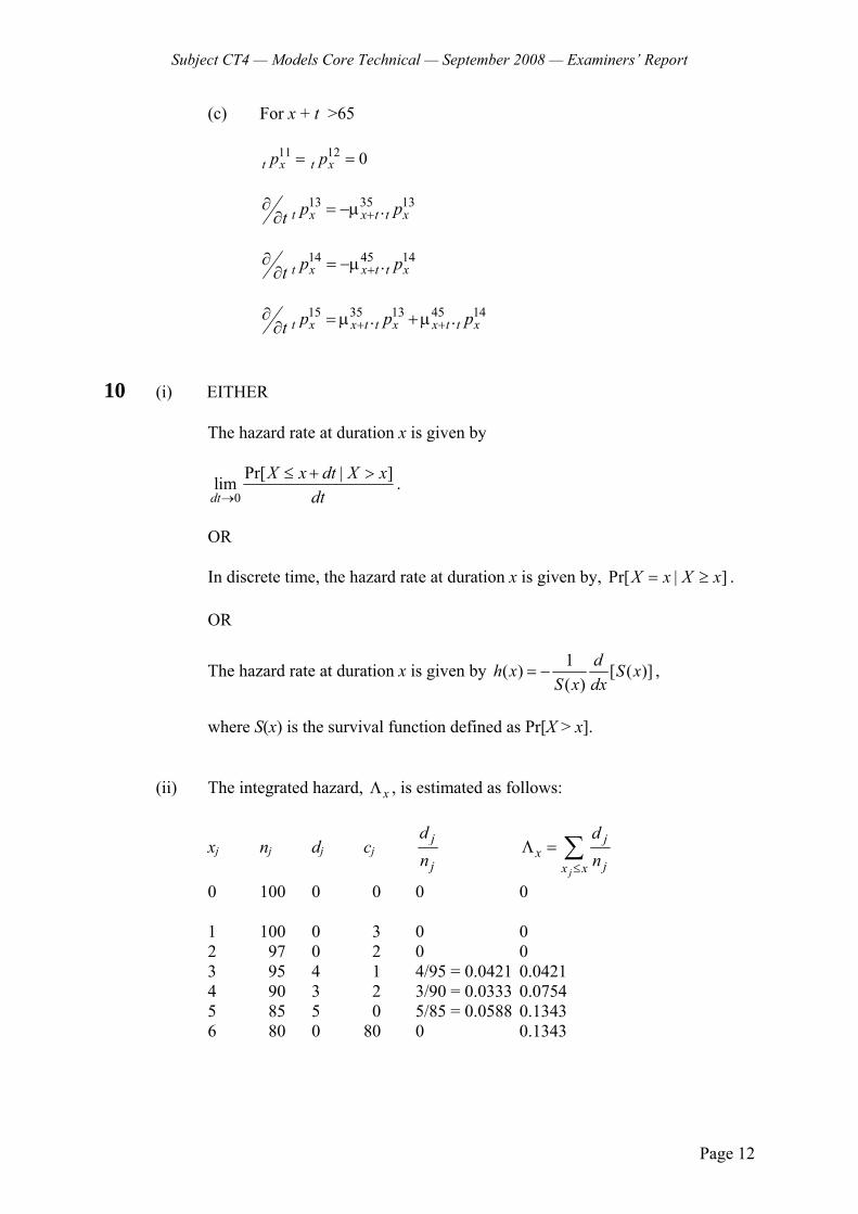
Subject CT4 — Models Core Technical — September 2008 — Examiners’ Report
Page 12
(c) For x + t >65
11 12 0t x t xp p= =
13 35 13.t x x t t xp pt +∂ = −μ∂
14 45 14.t x x t t xp pt +
∂ = −μ∂
15 35 13 45 14. .t x x t t x x t t xp p pt + +
∂ = μ +μ∂
10 (i) EITHER The hazard rate at duration x is given by
0
Pr[ | ]limdt
X x dt X xdt→
≤ + > .
OR
In discrete time, the hazard rate at duration x is given by, Pr[ | ]X x X x= ≥ . OR
The hazard rate at duration x is given by 1( ) [ ( )]( )
dh x S xS x dx
= − ,
where S(x) is the survival function defined as Pr[X > x]. (ii) The integrated hazard, xΛ , is estimated as follows:
xj nj dj cj j
j
dn
j
jx
jx x
dn≤
Λ = ∑
0 100 0 0 0 0
1 100 0 3 0 0 2 97 0 2 0 0 3 95 4 1 4/95 = 0.0421 0.0421 4 90 3 2 3/90 = 0.0333 0.0754 5 85 5 0 5/85 = 0.0588 0.1343 6 80 0 80 0 0.1343
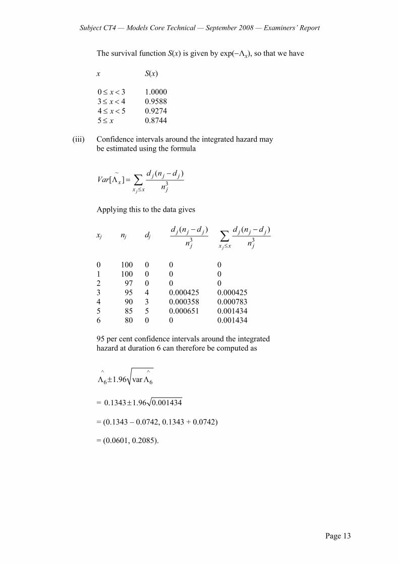
Subject CT4 — Models Core Technical — September 2008 — Examiners’ Report
Page 13
The survival function S(x) is given by exp(−Λx), so that we have x S(x) 0 3x≤ < 1.0000 3 4x≤ < 0.9588 4 5x≤ < 0.9274 5 x≤ 0.8744
(iii) Confidence intervals around the integrated hazard may be estimated using the formula
~
3
( )[ ]
j
j j jx
x x j
d n dVar
n≤
−Λ = ∑
Applying this to the data gives
xj nj dj 3
( )j j j
j
d n d
n
− 3
( )
j
j j j
x x j
d n d
n≤
−∑
0 100 0 0 0 1 100 0 0 0 2 97 0 0 0 3 95 4 0.000425 0.000425 4 90 3 0.000358 0.000783 5 85 5 0.000651 0.001434 6 80 0 0 0.001434 95 per cent confidence intervals around the integrated hazard at duration 6 can therefore be computed as
^ ^6 61.96 varΛ ± Λ
= 0.1343 1.96 0.001434± = (0.1343 – 0.0742, 0.1343 + 0.0742) = (0.0601, 0.2085).

Subject CT4 — Models Core Technical — September 2008 — Examiners’ Report
Page 14
THEN EITHER
The estimated survival function, ^( )S x is given
by ^
exp( )x−Λ ,
so that the 95 per cent confidence interval for ^( )S x is
[exp(−0.0601), exp(−0.2085)] which is (0.9417, 0.8118). In the previous investigation the probability that a prisoner would not be reconvicted within 6 months of release was 1 – 0.2 = 0.8.
Since the 95 per cent confidence interval around ^( )S x in the current
investigation does not include the value 0.8, and our estimate of ^( )S x > 0.8
we conclude that the rate of reconviction has declined since the previous investigation.
OR In the previous investigation the probability that a prisoner would not be reconvicted within 6 months of release was 1 – 0.2 = 0.8 – i.e. S(6) = 0.8 Since S(x) = exp(−Λx), the value of Λ6 corresponding to S(6) = 0.8 is Λ6 = −loge(0.8) = 0.2231.
Since this is higher than the upper limit in the range (0.0601, 0.2085) we conclude that the rate of reconviction has declined since the previous investigation.
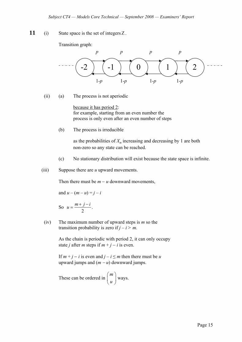
Subject CT4 — Models Core Technical — September 2008 — Examiners’ Report
Page 15
11 (i) State space is the set of integersΖ .
Transition graph:
(ii) (a) The process is not aperiodic because it has period 2: for example, starting from an even number the process is only even after an even number of steps
(b) The process is irreducible
as the probabilities of Xn increasing and decreasing by 1 are both
non-zero so any state can be reached.
(c) No stationary distribution will exist because the state space is infinite.
(iii) Suppose there are u upward movements.
Then there must be m − u downward movements,
and u – (m – u) = j – i
So 2
m j iu + −= .
(iv) The maximum number of upward steps is m so the
transition probability is zero if j – i > m. As the chain is periodic with period 2, it can only occupy state j after m steps if m + j − i is even. If m + j − i is even and j – i ≤ m then there must be u upward jumps and (m − u) downward jumps.
These can be ordered in mu
⎛ ⎞⎜ ⎟⎝ ⎠
ways.
-2 -1 0 1 2
p p p p
1-p 1-p 1-p 1-p
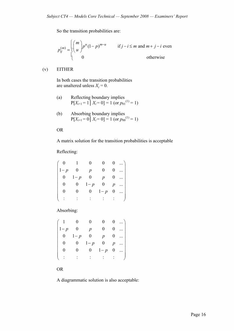
Subject CT4 — Models Core Technical — September 2008 — Examiners’ Report
Page 16
So the transition probabilities are:
( ) (1 ) if and even
0 otherwise
u m um
ij
mp p j i m m j i
p u−⎧⎛ ⎞
− − ≤ + −⎪⎜ ⎟= ⎨⎝ ⎠⎪⎩
(v) EITHER
In both cases the transition probabilities are unaltered unless Xi = 0. (a) Reflecting boundary implies P[Xi+1 = 1│Xi = 0] = 1 (or p01
(1) = 1)
(b) Absorbing boundary implies P[Xi+1 = 0│Xi = 0] = 1 (or p00
(1) = 1)
OR A matrix solution for the transition probabilities is acceptable
Reflecting:
0 1 0 0 0 ...1 0 0 0 ...
0 1 0 0 ...0 0 1 0 ...0 0 0 1 0 ...: : : : :
p pp p
p pp
⎛ ⎞⎜ ⎟−⎜ ⎟⎜ ⎟−⎜ ⎟
−⎜ ⎟⎜ ⎟−⎜ ⎟⎜ ⎟⎝ ⎠
Absorbing:
1 0 0 0 0 ...1 0 0 0 ...
0 1 0 0 ...0 0 1 0 ...0 0 0 1 0 ...: : : : :
p pp p
p pp
⎛ ⎞⎜ ⎟−⎜ ⎟⎜ ⎟−⎜ ⎟
−⎜ ⎟⎜ ⎟−⎜ ⎟⎜ ⎟⎝ ⎠
OR
A diagrammatic solution is also acceptable:
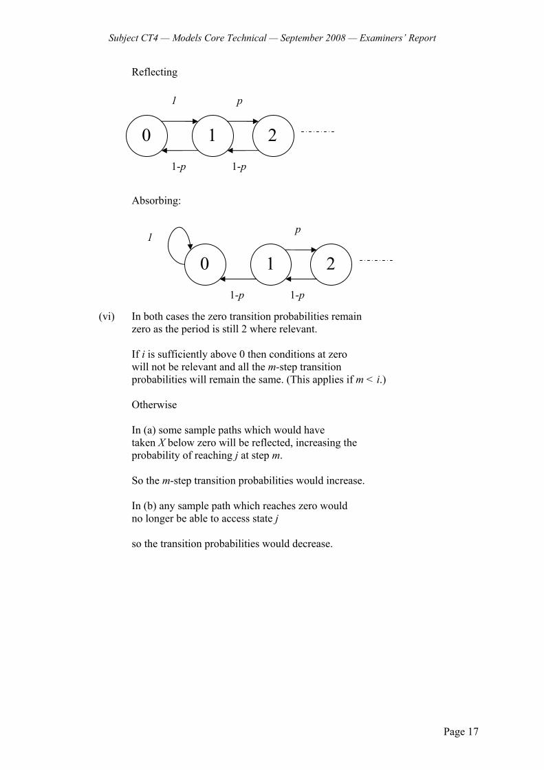
Subject CT4 — Models Core Technical — September 2008 — Examiners’ Report
Page 17
Reflecting
Absorbing:
(vi) In both cases the zero transition probabilities remain
zero as the period is still 2 where relevant. If i is sufficiently above 0 then conditions at zero will not be relevant and all the m-step transition probabilities will remain the same. (This applies if m < i.)
Otherwise In (a) some sample paths which would have taken X below zero will be reflected, increasing the probability of reaching j at step m. So the m-step transition probabilities would increase. In (b) any sample path which reaches zero would no longer be able to access state j so the transition probabilities would decrease.
0 1 2
p
1-p 1-p
1
0 1 2
1 p
1-p 1-p
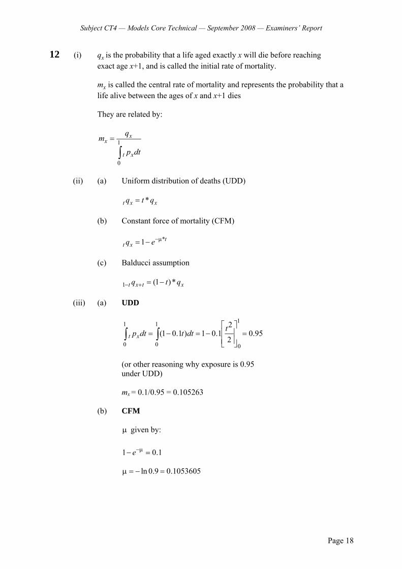
Subject CT4 — Models Core Technical — September 2008 — Examiners’ Report
Page 18
12 (i) qx is the probability that a life aged exactly x will die before reaching exact age x+1, and is called the initial rate of mortality.
mx is called the central rate of mortality and represents the probability that a life alive between the ages of x and x+1 dies
They are related by:
1
0
xx
t x
qm
p dt
=
∫
(ii) (a) Uniform distribution of deaths (UDD)
*t x xq t q= (b) Constant force of mortality (CFM) *1 t
t xq e−μ= −
(c) Balducci assumption 1 (1 )*t x t xq t q− + = −
(iii) (a) UDD
11 1
0 0 0
2(1 0.1 ) 1 0.1 0.95
2t xtp dt t dt⎡ ⎤⎢ ⎥= − = − =⎢ ⎥⎣ ⎦
∫ ∫
(or other reasoning why exposure is 0.95 under UDD) mx = 0.1/0.95 = 0.105263 (b) CFM
μ given by: 1 0.1e−μ− = ln 0.9 0.1053605μ = − =
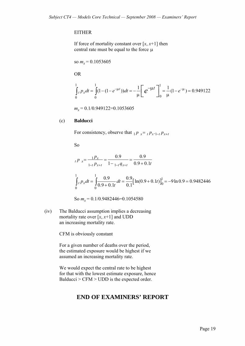
Subject CT4 — Models Core Technical — September 2008 — Examiners’ Report
Page 19
EITHER If force of mortality constant over [x, x+1] then central rate must be equal to the force μ
so mx = 0.1053605 OR
1 1 1
00 0
1 1(1 (1 )) (1 ) 0.949122tt x
tp dt e dt ee−μ −μ−μ= − − = − = − =μ μ⎡ ⎤∫ ∫ ⎣ ⎦
mx = 0.1/0.949122=0.1053605 (c) Balducci For consistency, observe that 1 1.x t x t x tp p p− += So
1
1 1
0.9 0.91 0.9 0.1
xt x
t x t t x t
ppp q t− + − +
= = =− +
[ ]1 1
10
0 0
0.9 0.9 ln(0.9 0.1 ) 9 ln 0.9 0.94824460.9 0.1 0.1t xp dt dt t
t= = + = − =
+∫ ∫ So mx = 0.1/0.9482446=0.1054580 (iv) The Balducci assumption implies a decreasing mortality rate over [x, x+1] and UDD an increasing mortality rate. CFM is obviously constant For a given number of deaths over the period, the estimated exposure would be highest if we assumed an increasing mortality rate. We would expect the central rate to be highest for that with the lowest estimate exposure, hence Balducci > CFM > UDD is the expected order.
END OF EXAMINERS’ REPORT

Faculty of Actuaries Institute of Actuaries
EXAMINATION
29 April 2009 (am)
Subject CT4 — Models Core Technical
Time allowed: Three hours
INSTRUCTIONS TO THE CANDIDATE
1. Enter all the candidate and examination details as requested on the front of your answer booklet.
2. You must not start writing your answers in the booklet until instructed to do so by the
supervisor. 3. Mark allocations are shown in brackets. 4. Attempt all 12 questions, beginning your answer to each question on a separate sheet. 5. Candidates should show calculations where this is appropriate.
Graph paper is not required for this paper.
AT THE END OF THE EXAMINATION
Hand in BOTH your answer booklet, with any additional sheets firmly attached, and this question paper.
In addition to this paper you should have available the 2002 edition of the Formulae and Tables and your own electronic calculator from the approved list.
© Faculty of Actuaries CT4 A2009 © Institute of Actuaries

CT4 A2009—2
1 A life insurance company has a small group of policies written on impaired lives and has conducted an investigation into the mortality of these policyholders. It is proposed that the crude mortality rates be graduated for use in future premium calculations.
Discuss the suitability of two methods of graduation that the insurance company could
use. [3] 2 (i) Explain what is meant by a time-homogeneous Markov chain. [2] Consider the time-homogeneous two-state Markov chain with transition matrix:
1
1a a
b b−⎛ ⎞
⎜ ⎟−⎝ ⎠
(ii) Explain the range of values that a and b can take which result in this being a
valid Markov chain which is:
(a) irreducible (b) periodic [3]
[Total 5]
3 List the benefits and limitations of modelling in actuarial work. [5] 4 Below is an extract from English Life Table 15 (females). Age x Number of survivors to (years) exact age x out of 100,000 births 30 98,617 40 97,952 (i) Calculate 5 30q under each of the two following alternative assumptions:
(a) a uniform distribution of deaths (UDD) between ages 30 and 40 years (b) a constant force of mortality between ages 30 and 40 years [3]
(ii) Calculate the number of survivors to exact age 35 years out of 100,000 births
under each of the assumptions in (i) above. [1] English Life Table 15 (females) was originally calculated using data classified by
single years of age. The number of survivors to exact age 35 years was 98,359.
(iii) Comment on the appropriateness of the assumptions of UDD and a constant force of mortality between ages 30 and 40 years in this example. [3]
[Total 7]
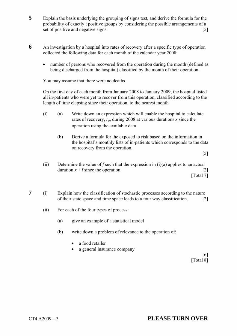
CT4 A2009—3 PLEASE TURN OVER
5 Explain the basis underlying the grouping of signs test, and derive the formula for the probability of exactly t positive groups by considering the possible arrangements of a set of positive and negative signs. [5]
6 An investigation by a hospital into rates of recovery after a specific type of operation
collected the following data for each month of the calendar year 2008:
• number of persons who recovered from the operation during the month (defined as being discharged from the hospital) classified by the month of their operation.
You may assume that there were no deaths.
On the first day of each month from January 2008 to January 2009, the hospital listed
all in-patients who were yet to recover from this operation, classified according to the length of time elapsing since their operation, to the nearest month. (i) (a) Write down an expression which will enable the hospital to calculate
rates of recovery, rx, during 2008 at various durations x since the operation using the available data.
(b) Derive a formula for the exposed to risk based on the information in
the hospital’s monthly lists of in-patients which corresponds to the data on recovery from the operation. [5]
(ii) Determine the value of f such that the expression in (i)(a) applies to an actual
duration x + f since the operation. [2] [Total 7] 7 (i) Explain how the classification of stochastic processes according to the nature
of their state space and time space leads to a four way classification. [2] (ii) For each of the four types of process:
(a) give an example of a statistical model (b) write down a problem of relevance to the operation of:
• a food retailer • a general insurance company [6]
[Total 8]
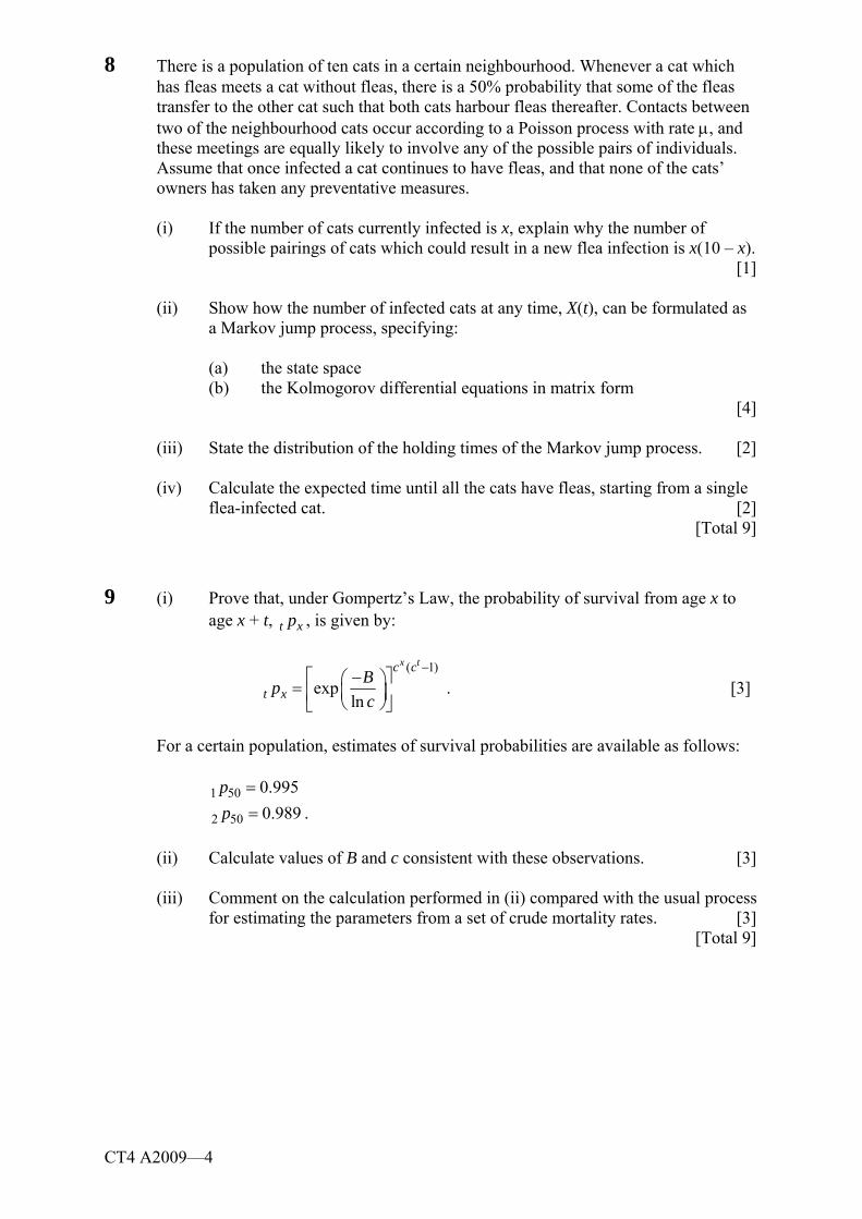
CT4 A2009—4
8 There is a population of ten cats in a certain neighbourhood. Whenever a cat which has fleas meets a cat without fleas, there is a 50% probability that some of the fleas transfer to the other cat such that both cats harbour fleas thereafter. Contacts between two of the neighbourhood cats occur according to a Poisson process with rate μ, and these meetings are equally likely to involve any of the possible pairs of individuals. Assume that once infected a cat continues to have fleas, and that none of the cats’ owners has taken any preventative measures.
(i) If the number of cats currently infected is x, explain why the number of
possible pairings of cats which could result in a new flea infection is x(10 – x). [1] (ii) Show how the number of infected cats at any time, X(t), can be formulated as
a Markov jump process, specifying:
(a) the state space (b) the Kolmogorov differential equations in matrix form
[4] (iii) State the distribution of the holding times of the Markov jump process. [2] (iv) Calculate the expected time until all the cats have fleas, starting from a single
flea-infected cat. [2] [Total 9] 9 (i) Prove that, under Gompertz’s Law, the probability of survival from age x to age x + t, t xp , is given by:
( 1)
expln
x tc c
t xBpc
−⎡ ⎤−⎛ ⎞= ⎜ ⎟⎢ ⎥⎝ ⎠⎣ ⎦
. [3]
For a certain population, estimates of survival probabilities are available as follows: 1 50 0.995p = 2 50 0.989p = . (ii) Calculate values of B and c consistent with these observations. [3] (iii) Comment on the calculation performed in (ii) compared with the usual process
for estimating the parameters from a set of crude mortality rates. [3] [Total 9]
CT4 A2009—5 PLEASE TURN OVER
10 Let Tx be a random variable denoting future lifetime after age x, and let T be another random variable denoting the lifetime of a new-born person.
(i) (a) Define, in terms of probabilities, ( )xS t , which represents the survival function of Tx.
(b) Derive an expression relating ( )xS t to ( )S t , the survival function of T. [2]
(ii) Define, in terms of probabilities involving Tx , the force of mortality, x t+μ . [1] The Weibull distribution has a survival function given by ( )( ) exp ( )xS t t β= − λ ,
where λ and β are parameters (λ, β > 0). (iii) Derive an expression for the Weibull force of mortality in terms of λ and β. [3] (iv) Sketch, on the same graph, the Weibull force of mortality for 0 5t≤ ≤ for the
following pairs of values of λ and β: λ = 1, β = 0.5 λ = 1, β = 1.0 λ = 1, β = 1.5 [4] [Total 10]
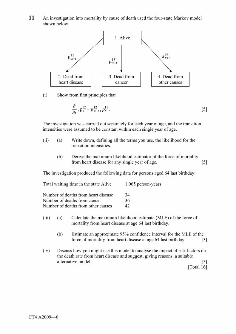
CT4 A2009—6
11 An investigation into mortality by cause of death used the four-state Markov model shown below.
(i) Show from first principles that
12 12 11t x x t t xp p
t +∂
= μ∂
. [5]
The investigation was carried out separately for each year of age, and the transition
intensities were assumed to be constant within each single year of age. (ii) (a) Write down, defining all the terms you use, the likelihood for the
transition intensities. (b) Derive the maximum likelihood estimator of the force of mortality
from heart disease for any single year of age. [5] The investigation produced the following data for persons aged 64 last birthday: Total waiting time in the state Alive 1,065 person-years Number of deaths from heart disease 34 Number of deaths from cancer 36 Number of deaths from other causes 42
(iii) (a) Calculate the maximum likelihood estimate (MLE) of the force of
mortality from heart disease at age 64 last birthday. (b) Estimate an approximate 95% confidence interval for the MLE of the
force of mortality from heart disease at age 64 last birthday. [3]
(iv) Discuss how you might use this model to analyse the impact of risk factors on the death rate from heart disease and suggest, giving reasons, a suitable alternative model. [3]
[Total 16]
1 Alive
2 Dead from heart disease
3 Dead from cancer
4 Dead from other causes
12x t+μ 13
x t+μ
14x t+μ
CT4 A2009—7
12 A motor insurer operates a no claims discount system with the following levels of discount {0%, 25%, 50%, 60%}.
The rules governing a policyholder’s discount level, based upon the number of claims
made in the previous year, are as follows:
• Following a year with no claims, the policyholder moves up one discount level, or remains at the 60% level.
• Following a year with one claim, the policyholder moves down one discount level,
or remains at 0% level. • Following a year with two or more claims, the policyholder moves down two
discount levels (subject to a limit of the 0% discount level). The number of claims made by a policyholder in a year is assumed to follow a
Poisson distribution with mean 0.30. (i) Determine the transition matrix for the no claims discount system. [3] (ii) Calculate the stationary distribution of the system, π . [5] (iii) Calculate the expected average long term level of discount. [1] The following data shows the number of the insurer’s 130,200 policyholders in the
portfolio classified by the number of claims each policyholder made in the last year. This information was used to estimate the mean of 0.30.
No claims 96,632 One claim 28,648 Two claims 4,400 Three claims 476 Four claims 36 Five claims 8 (iv) Test the goodness of fit of these data to a Poisson distribution with mean 0.30.
[5] (v) Comment on the implications of your conclusion in (iv) for the average level
of discount applied. [2] [Total 16]
END OF PAPER

Faculty of Actuaries Institute of Actuaries
Subject CT4 — Models Core Technical
EXAMINERS’ REPORT
April 2009
Introduction The attached subject report has been written by the Principal Examiner with the aim of helping candidates. The questions and comments are based around Core Reading as the interpretation of the syllabus to which the examiners are working. They have however given credit for any alternative approach or interpretation which they consider to be reasonable. R D Muckart Chairman of the Board of Examiners June 2009
© Faculty of Actuaries © Institute of Actuaries

Subject CT4 — Models Core Technical — April 2009 — Examiners’ Report
Page 2
Comments Comments on solutions presented to individual questions for the April 2009 paper are given below. Q1 Answers to this question were satisfactory. Most candidates realised that graduation by reference to a standard table was potentially appropriate, and that graphical graduation might have to be used as a last resort. Credit was given for sensible points other than those mentioned in the specimen solution below. Q2 In part (ii) some explanation of the correct possible values of a and b was required for full credit. A common error in part (ii) (a) was to write 0 < a < 1 and 0 < b < 1, ignoring the possibility that a and b could equal 1. Q3 This bookwork question was well answered by many candidates. Credit was given for sensible points other than those mentioned in the specimen solution below. Q4 Answers to parts (i) and (ii) were generally good, with a substantial proportion of candidates scoring full marks. Part (iii) was much less convincingly answered. Although not all the points mentioned in the specimen solutions below were required for full credit, many candidates only included the briefest of comments, and consequently scored few marks. Q5 Most candidates simply wrote down the formula for Pr[G=t] (which is given in the book of Formulae and Tables) and then explained what each bracketed expression in the formula meant. Few candidates gave more than the briefest explanation of why the test is useful, and what it is designed to achieve, and still fewer gave any indication of how the test was to be performed. Q6 Answers to this question were very disappointing. Although this was slightly more demanding than some exposed-to-risk questions in the past, many candidates seemed to have little notion of how to approximate the central exposed to risk. Q7 This question was generally well answered, although part (ii) was less well answered than similar questions on previous papers in which examples relevant to actuarial work were asked for. Marks were deducted in part (ii) for problems which seemed trivial, or where essentially the same examples were given for more than one class of models. Q8 Few candidates made a serious attempt at this question. Many answers consisted of an attempt at part (i) followed by a description of the state space in part (ii)(a), the general expression for the Kolmogorov equations, and a statement in part (iii) that the distribution of holding times was exponential. Few candidates attempted to write down the matrix in part (ii). Note that credit was given in part (iv) for errors carried forward from incorrect matrices in part (ii). Q9 Part (i) of this question was well answered by a good proportion of candidates. Fewer managed to calculate the values of B and c in part (ii), partly due to algebraic errors. Credit was given for the calculation of B to candidates who calculated an incorrect value for c but then correctly computed the value of B which corresponded to their value of c. Part (iii) was poorly answered, with many candidates offering no comments at all.
Subject CT4 — Models Core Technical — April 2009 — Examiners’ Report
Page 3
Q10 Answers to this question were very disappointing. Parts (i) and (ii) were bookwork based on the Core Reading, yet many candidates seemed not to understand what was required. Part (iii) was rather better answered. Candidates who derived an incorrect hazard function in part (iii) could score full credit in part (iv) for correct sketches of these incorrect hazards. Indeed, of the relatively small number of candidates who scored highly for the sketches in part (iv), some did indeed produce correct plots of incorrect (and sometimes much more complicated) hazard functions. Q11 This question was well answered by many candidates. The only general weaknesses were steps missing in part (i) and the lack of explanation of where the approximate variance came from in part (iii)(b). In part (iv), an encouraging number of candidates realised that the Cox model was an obvious alternative model, though few made any further comments on how it might be applied to the problem mentioned in the question. Q12 This question was also well answered by the majority of candidates. Many scored full marks on parts (i), (ii) and (iii), and made a good attempt at part (iv). The comments asked for in part (v) were, however, much less convincingly made. In part (iv), several candidates combined the two categories “4 claims” and “5 claims” because the expected value was small. Full credit was given for this if the chi-squared statistic was computed correctly, and the number of degrees of freedom was correct for this alternative. However, candidates who performed the test on the reduced number of categories “0 claims”, “1 claim” and “2 or more claims” were penalised.
Subject CT4 — Models Core Technical — April 2009 — Examiners’ Report
Page 4
1 Graduation by reference to a standard table might be appropriate, if a suitable standard table could be found.
However the fact that the company insures non-standard lives makes it unlikely that a
suitable standard table would exist.
Graphical graduation might be used if no suitable standard table can be found.
However it is a last resort as it is difficult to obtain results which are smooth and which adhere to the data.
Graduation using a parametric formula is unlikely to be appropriate as the amount of
data in this investigation is likely to be small and it is unlikely that the company will want to produce a standard table.
2 (i) A Markov chain is a stochastic process with discrete states operating in
discrete time in which the probabilities of moving from one state to another are dependent only on the present state of the process.
EITHER If the transition probabilities are also independent of time. OR If the l-step transition probabilities are dependent only on the time lag, the
chain is said to be time-homogeneous. (ii) (a) In this case the chain is irreducible if the transition probability
out of each state is non-zero (or, equivalently, if it is possible to reach the other state from both states)
So requires 0 1a< ≤ and 0 1b< ≤
(b) The chain is only periodic if the chain must alternate between the states. So a = 1 and b = 1.

Subject CT4 — Models Core Technical — April 2009 — Examiners’ Report
Page 5
3 Benefits Complex systems with stochastic elements can be studied. Different future policies or possible actions can be compared. In models of complex systems we can control the experimental conditions and thus
reduce the variance of the results without upsetting their mean values.
Can calibrate to observed data and hence model interdependencies between outcomes. Often models are the only practicable means of answering actuarial questions. Systems with a long time-frame can be studied and results obtained relatively quickly.
Limitations Time or cost or resources required for model development. In a stochastic model, many independent runs of the model are needed to obtain
results for a given set of inputs. Models can look impressive and there is a danger this results in false sense of
confidence. Poor or incredible data input or assumptions will lead to flawed output. Users need to understand the model and the uses to which it can safely be put — the
model is not a “black box”. It is not possible to include all future events in a model (e.g. change in legislation).
Interpreting the results can be a challenge. Any model will be an approximation.
Models are better for comparing the impact of input variations than for optimising outputs.
Subject CT4 — Models Core Technical — April 2009 — Examiners’ Report
Page 6
4 (i) (a) Under UDD the number of deaths between exact ages 30 and 35 years is half the number of deaths between exact ages 30 and 40 years.
So the number of deaths between exact ages 30 and 35 years is ½(98,617 – 97,952) = 332.5
and 5 30332.5 0.0033716
98,617q = = .
(b) Let the constant force of mortality be µ.
Then, since 0
expt
t x x sp ds+
⎛ ⎞⎜ ⎟= − μ⎜ ⎟⎝ ⎠∫ ,
( )10 30 exp 10p = − μ so
( ) ( )10 30 log 97,952 / 98,617log0.0006766
10 10ee p −−
μ = = = .
5 30 5 301 1 exp( 5 )q p= − = − − μ 1 exp[( 5)(0.0006766)] 0.0033773= − − = . (ii) EITHER The number of survivors to exact age 35 years is 5 30 5 3098,617 98,617(1 )p q= − , so for UDD this is 98,617(1 0.0033716) 98,284.5− = , and under a constant force of mortality this is 98,617(1 0.0033773) 98,283.9− = . OR Under UDD the number of survivors to exact age 35 years is (98,617 + 97,952)/2 = 98,284.5.

Subject CT4 — Models Core Technical — April 2009 — Examiners’ Report
Page 7
Under a constant force of mortality the number of survivors to exact age 35 years is given by 98,617*97,952 98, 283.9= (iii) The actual number of survivors to exact age 35 years is higher (or,
equivalently, mortality is lighter) than that under either the UDD or the constant force assumptions.
The actual number of survivors implies that there were 258 deaths between
ages 30 and 35 years and 407 deaths between ages 35 and 40 years.
The actual data reveal that the force of mortality is higher between ages 35 and
40 years than it is between ages 30 and 35 years for females in English Life Table 15, which suggests that the force of mortality is increasing over this age
range. The assumption of UDD implies an increasing force of mortality.
The actual force of mortality seems to be increasing even faster than is implied
by UDD. A constant force of mortality is unlikely to be realistic for this age range. Used over a 10-year age span the assumption of UDD is unlikely to be appropriate, whereas used over single years of age it is acceptable. 5 Suppose we have a set of n crude mortality rates for a given age range x to x + n − 1,
and we wish to compare them to a standard set of n mortality rates for the same age range.
If the mortality underlying the crude rates is the same as that of the standard set of
rates (the null hypothesis), then we should expect the difference between the two sets of rates to be due only to sampling variability.
The grouping of signs test tests the null hypothesis by examining the number of groups of consecutive positive deviations among the n ages, where a positive deviation occurs when the crude rate exceeds the corresponding rate in the standard set.
Suppose there are a total of m positive deviations, n – m negative deviations and G
positive groups. Then the number of possible ways to arrange t positive groups among n – m negative
deviations is 1n m
t− +⎛ ⎞
⎜ ⎟⎝ ⎠
.
Subject CT4 — Models Core Technical — April 2009 — Examiners’ Report
Page 8
There are 1
1mt−⎛ ⎞
⎜ ⎟−⎝ ⎠ways to arrange m positive signs into t positive groups.
There are nm⎛ ⎞⎜ ⎟⎝ ⎠
ways to arrange m positive and n – m negative signs.
Therefore the probability of exactly t positive groups is
1 11
Pr[ ]
n m mt t
G tnm
− + −⎛ ⎞⎛ ⎞⎜ ⎟⎜ ⎟−⎝ ⎠⎝ ⎠= =
⎛ ⎞⎜ ⎟⎝ ⎠
The grouping of signs test then evaluates Pr[ ]t G≤ under the null hypothesis.
If this is less than 0.05 we reject the null hypothesis at the 5% level. 6 (i) (a) The relevant recovery rates can be estimated as
xx c
x
drE
= , x = 0, 1, 2, ... months
where dx is the number of persons recovering in the calendar month
that was x months after the calendar month of their operation, and cxE is
the central exposed to risk. (b) We need to ensure that the c
xE correspond to the data on persons recovering
The hospital’s data imply a calendar month rate interval for the
recoveries, running from the first day of each month until the last day of each month.
Using the monthly “census” data, a definition of c
xE which corresponds to the deaths data can be obtained as follows.
We observe ,x tP = number of lives under observation for whom the
time elapsing since the operation was between x − ½ and x + ½ months, where t is the time in months since 1 January 2008.
Subject CT4 — Models Core Technical — April 2009 — Examiners’ Report
Page 9
Therefore, using the census formula:
( )12 11
, , 1, 100
1* * *2cx x t x t x tE P dt P P + += = +∑∫ ,
where , 1, ,
1* ( )2x t x t x tP P P−= + .
We assume all months are the same length, and that the numbers in the
hospital vary linearly across each month. (ii) At the start of the rate interval, durations since the operation range from x − 1
to x months, so the average duration is x − ½, assuming operations take place evenly across the month.
rx estimates the recovery rate at the mid-point of the rate interval. This is exactly x months since the operation, so f = 0. 7 (i) Processes can be classified, first, according to whether their state space (i.e.
the range of states they can possibly occupy) is discrete or continuous
For processes operating in both discrete and continuous state space the time domain can either be discrete or continuous
Therefore we have four possible types of process EITHER 2 types of state space × 2 types of time domain OR State space Time domain Discrete Discrete Discrete Continuous Continuous Discrete Continuous Continuous

Subject CT4 — Models Core Technical — April 2009 — Examiners’ Report
Page 10
(ii) Type of process Statistical model Problem of relevance
to food retailer Problem of relevance to a general insurer
SS Discrete/ T Discrete
Markov chain Markov jump chain Counting process Random walk
Whether or not particular product out of stock at the end of each day
No claims bonus
SS Discrete/ T Continuous
Counting process Poisson process Markov jump processCompound Poisson process
Rate of arrival of customers in shop
Number of claims received monitored continuously
SS Continuous/ T Discrete
ARIMA time series model General random walk White noise
Value of goods in stock at the end of each day
Total amount insured on a certain type of policy valued at the end of each month
SS Continuous/ T Continuous
Compound Poisson process Brownian motion Ito process
Volume (or value) of trade in shop over a continuous period of time
Value of claims arriving monitored continuously
8 (i) There are x infected cats and hence 10 – x uninfected cats. Flea transmission requires one of the x infected cats to meet one of the (10 − x)
uninfected cats.
(ii) The total number of pairings of cats is 102
⎛ ⎞⎜ ⎟⎝ ⎠
= 45.
So the probability of a meeting resulting in an increase in the number of cats
with fleas is 0.5x(10 − x)/45. As this depends only on the number of cats currently infected, and meetings
occur according to a Poisson process, the number of infected cats over time follows a Markov jump process.
(a) The state space is the number of cats infected {0,1,2,,…..10}
Subject CT4 — Models Core Technical — April 2009 — Examiners’ Report
Page 11
(b) The generator matrix is
0 09 9
16 1621 21
24 2425 25
9024 24
21 2116 16
9 90
A
⎛ ⎞⎜ ⎟−⎜ ⎟⎜ ⎟−⎜ ⎟
−⎜ ⎟⎜ ⎟−⎜ ⎟μ
= −⎜ ⎟⎜ ⎟−⎜ ⎟
−⎜ ⎟⎜ ⎟−⎜ ⎟⎜ ⎟−⎜ ⎟⎝ ⎠
Kolmogorov’s equations: EITHER
forward form ( ) ( )d P t P t Adt
=
OR
backward form ( ) ( )d P t AP tdt
=
(iii) Holding times are exponentially distributed.
With mean 90(10 )x xμ −
OR parameter (10 )90
x xμ − .
(iv) Total expected time is the sum of the mean holding times.
9
1
90 1 90 1 1 1 1 1 1 1 1 1(10 ) 9 16 21 24 25 24 21 16 9x x x=
⎛ ⎞= = + + + + + + + +⎜ ⎟μ − μ ⎝ ⎠∑
= 50.92/µ
Subject CT4 — Models Core Technical — April 2009 — Examiners’ Report
Page 12
9 (i) Under Gompertz’s Law x
x Bcμ = . Since
0
expt
t x x wp dw+
⎛ ⎞⎜ ⎟= − μ⎜ ⎟⎝ ⎠∫ ,
we have 0 0
exp expln
tt x wx w
t xBc cp Bc dw
c+
⎛ ⎞⎛ ⎞⎜ ⎟⎜ ⎟= − = −
⎜ ⎟ ⎜ ⎟⎝ ⎠ ⎝ ⎠∫ ,
which is expln
x t xBc c Bc
c
⎛ ⎞⎡ ⎤−⎣ ⎦⎜ ⎟− =⎜ ⎟⎝ ⎠
( 1)
expln
x tc cBc
−⎡ ⎤−⎛ ⎞
⎜ ⎟⎢ ⎥⎝ ⎠⎣ ⎦.
(ii) Define Q = 50
expln
cBc
⎡ ⎤−⎛ ⎞⎜ ⎟⎢ ⎥⎝ ⎠⎣ ⎦
ln 0.995 = (c − 1) ln Q ln 0.989 = (c2 − 1) ln Q
2( 1) ( 1)( 1) 2.20665
( 1) ( 1)c c cc c− − +
= =− −
c = 1.20665 Therefore Q = 0.976036128
501.20665
exp 0.976036128ln1.20665
B⎡ ⎤−⎛ ⎞ =⎜ ⎟⎢ ⎥⎝ ⎠⎣ ⎦
B = 3.797*10−7. (iii) In this example, only two observations are provided so there is an analytical
solution to the Gompertz model. This is unrealistic as in general a graduation process would be used to provide
a fit to a set of crude rates. This could be done by weighted least squares or maximum likelihood.
Subject CT4 — Models Core Technical — April 2009 — Examiners’ Report
Page 13
The more general graduation process allows the fitting of more complex models from the Gompertz-Makeham family which have the form
xμ = polynomial(1) + exp(polynomial(2)) the parameters of which cannot always so easily be estimated by the method
used in part (ii). 10 (i) (a) ( ) Pr[ ]x xS t T t= > (b) EITHER
Since Pr[ ]Pr[ ] Pr[ | ]Pr[ ]x
T x tT t T x t T xT x> +
> = > + > =>
and ( ) Pr[ ]S t T t= > ,
then ( )( )( )x
S x tS tS x+
= .
OR
Since ( )x t xS t p= , then using the consistency principle
0 0.x t t x xp p p+ =
Therefore 0
0( ) x t
t x xx
pp S tp
+= = =( )
( )S x t
S x+ .
(ii) EITHER
1 [Pr( )]Pr[ ]x t x
x
d T tT t dt+μ = − >
>
OR
( )0
1lim Pr[ |x t x xh
T t h T th++
→μ = ≤ + >
(iii) EITHER
If the density function of Tx is ( )xf t , then we can write
( ) ( ) ( )x x x t xdf t S t S tdt+= μ = −
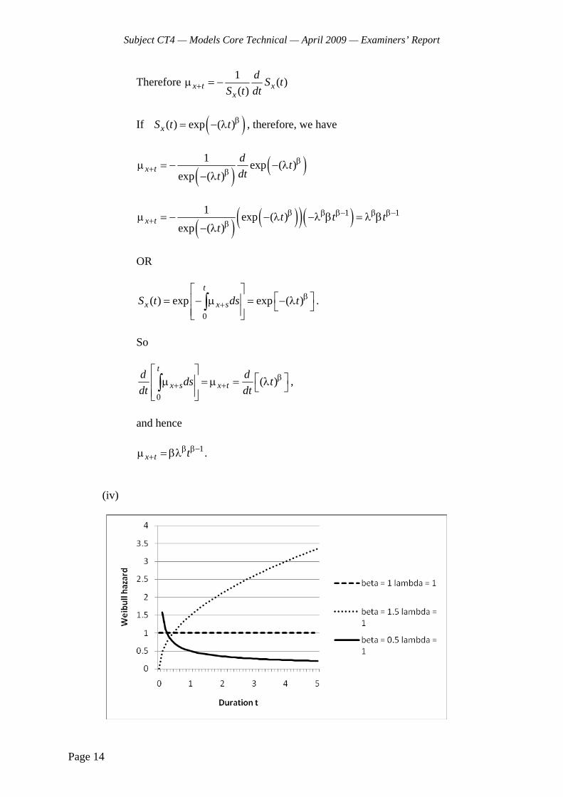
Subject CT4 — Models Core Technical — April 2009 — Examiners’ Report
Page 14
Therefore 1 ( )( )x t x
x
d S tS t dt+μ = −
If ( )( ) exp ( )xS t t β= − λ , therefore, we have
( ) ( )1 exp ( )
exp ( )x t
d tdtt
β+ β
μ = − − λ− λ
( ) ( )( )( )1 11 exp ( )
exp ( )x t t t t
tβ β β− β β−
+ βμ = − − λ −λ β = λ β
− λ
OR
0
( ) exp exp ( )t
x x sS t ds t β+
⎡ ⎤⎡ ⎤⎢ ⎥= − μ = − λ⎣ ⎦⎢ ⎥⎣ ⎦
∫ .
So
0
( )t
x s x td dds tdt dt
β+ +
⎡ ⎤⎡ ⎤⎢ ⎥μ = μ = λ⎣ ⎦⎢ ⎥⎣ ⎦
∫ ,
and hence 1
x t tβ β−+μ = βλ .
(iv)

Subject CT4 — Models Core Technical — April 2009 — Examiners’ Report
Page 15
11 (i) Condition on the state occupied at t. We have 12 11 12 12 22
t dt x t x dt x t t x dt x tp p p p p+ + += + . since it is impossible to leave states 3 and 4 once entered. Also, 22
dt x tp + = 1, since state 2 is an absorbing state. We now assume that, for small dt, 12 12 ( )dt x t x tp dt o dt+ += μ + where o(dt) is the probability that a life makes two or more transitions in the
time interval dt, and
0
( )lim 0dt
o dtdt→
= .
Substituting for 12
dt x tp + gives 12 12 11 12 ( )t dt x x t t x t xp p dt p o dt+ += μ + + Thus 12 12 12 11 ( )t dt x t x x t t xp p p dt o dt+ +− = μ + and
12 12
12 12 11
0lim t dt x t x
t x x t t xdt
p pp pt dt+
++
→
−∂= = μ
∂
(ii) (a) Suppose we observe d12 deaths from heart disease, d13 deaths from
cancer and d14 deaths from other causes.
Suppose also that we observe the waiting time for each life, and that the total observed waiting time is V, being the sum of the waiting times for each life.
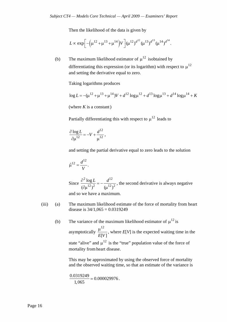
Subject CT4 — Models Core Technical — April 2009 — Examiners’ Report
Page 16
Then the likelihood of the data is given by
( ) 12 13 1412 13 14 12 13 14exp ( ) ( ) ( ) .d d dL V⎡ ⎤∝ − μ +μ +μ μ μ μ⎣ ⎦
(b) The maximum likelihood estimator of 12μ is obtained by
differentiating this expression (or its logarithm) with respect to 12μ and setting the derivative equal to zero.
Taking logarithms produces 12 13 14 12 12 13 13 14 14log ( ) log log logL V d d d K= − μ +μ +μ + μ + μ + μ + (where K is a constant ) Partially differentiating this with respect to 12μ leads to
12
12 12log L dV∂
= − +∂μ μ
,
and setting the partial derivative equal to zero leads to the solution
12
12ˆ .dV
μ =
Since 2 12
12 2 12 2log
( ) ( )L d∂= −
∂μ μ, the second derivative is always negative
and so we have a maximum. (iii) (a) The maximum likelihood estimate of the force of mortality from heart
disease is 34/1,065 = 0.0319249
(b) The variance of the maximum likelihood estimator of 12μ is
asymptotically 12
[ ]E Vμ , where E[V] is the expected waiting time in the
state “alive” and 12μ is the “true” population value of the force of mortality from heart disease.
This may be approximated by using the observed force of mortality and the observed waiting time, so that an estimate of the variance is
0.0319249 0.0000299761,065
= .
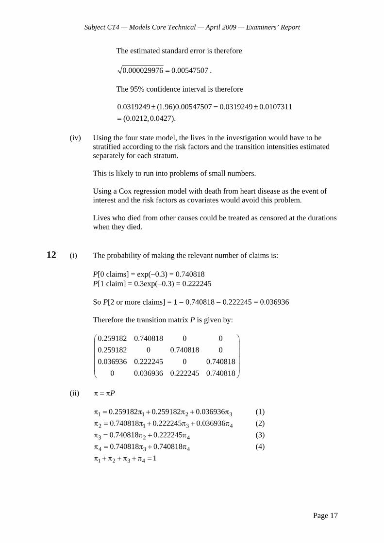
Subject CT4 — Models Core Technical — April 2009 — Examiners’ Report
Page 17
The estimated standard error is therefore 0.000029976 0.00547507= . The 95% confidence interval is therefore
0.0319249 (1.96)0.00547507 0.0319249 0.0107311
(0.0212,0.0427).± = ±
=
(iv) Using the four state model, the lives in the investigation would have to be
stratified according to the risk factors and the transition intensities estimated separately for each stratum.
This is likely to run into problems of small numbers. Using a Cox regression model with death from heart disease as the event of
interest and the risk factors as covariates would avoid this problem.
Lives who died from other causes could be treated as censored at the durations when they died.
12 (i) The probability of making the relevant number of claims is: P[0 claims] = exp(−0.3) = 0.740818 P[1 claim] = 0.3exp(−0.3) = 0.222245 So P[2 or more claims] = 1 − 0.740818 − 0.222245 = 0.036936 Therefore the transition matrix P is given by:
0.259182 0.740818 0 00.259182 0 0.740818 00.036936 0.222245 0 0.740818
0 0.036936 0.222245 0.740818
⎛ ⎞⎜ ⎟⎜ ⎟⎜ ⎟⎜ ⎟⎝ ⎠
(ii) Pπ = π 1 1 2 30.259182 0.259182 0.036936π = π + π + π (1) 2 1 3 40.740818 0.222245 0.036936π = π + π + π (2) 3 2 40.740818 0.222245π = π + π (3) 4 3 40.740818 0.740818π = π + π (4) 1 2 3 4 1π + π + π + π =
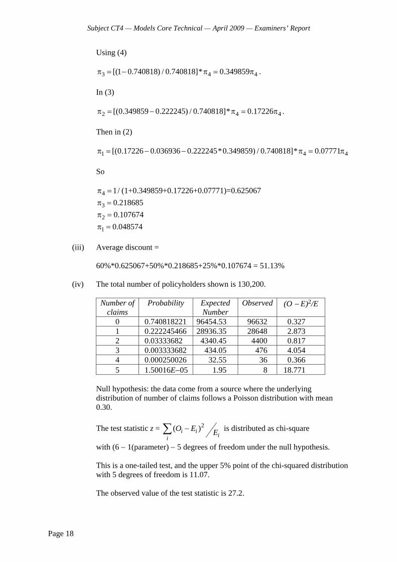
Subject CT4 — Models Core Technical — April 2009 — Examiners’ Report
Page 18
Using (4) 3 4 4[(1 0.740818) / 0.740818]* 0.349859π = − π = π .
In (3) 2 4 4[(0.349859 0.222245) / 0.740818]* 0.17226π = − π = π . Then in (2) 1 4 4[(0.17226 0.036936 0.222245*0.349859) / 0.740818]* 0.07771π = − − π = π So 4 1/π = (1+0.349859+0.17226+0.07771)=0.625067 3 0.218685π = 2 0.107674π = 1 0.048574π = (iii) Average discount = 60%*0.625067+50%*0.218685+25%*0.107674 = 51.13% (iv) The total number of policyholders shown is 130,200.
Number of claims
Probability Expected Number
Observed (O − E)2/E
0 0.740818221 96454.53 96632 0.327 1 0.222245466 28936.35 28648 2.873 2 0.03333682 4340.45 4400 0.817 3 0.003333682 434.05 476 4.054 4 0.000250026 32.55 36 0.366 5 1.50016E−05 1.95 8 18.771
Null hypothesis: the data come from a source where the underlying distribution of number of claims follows a Poisson distribution with mean 0.30.
The test statistic z = 2( )i i
iiO E E−∑ is distributed as chi-square
with (6 − 1(parameter) − 5 degrees of freedom under the null hypothesis. This is a one-tailed test, and the upper 5% point of the chi-squared distribution with 5 degrees of freedom is 11.07.
The observed value of the test statistic is 27.2.
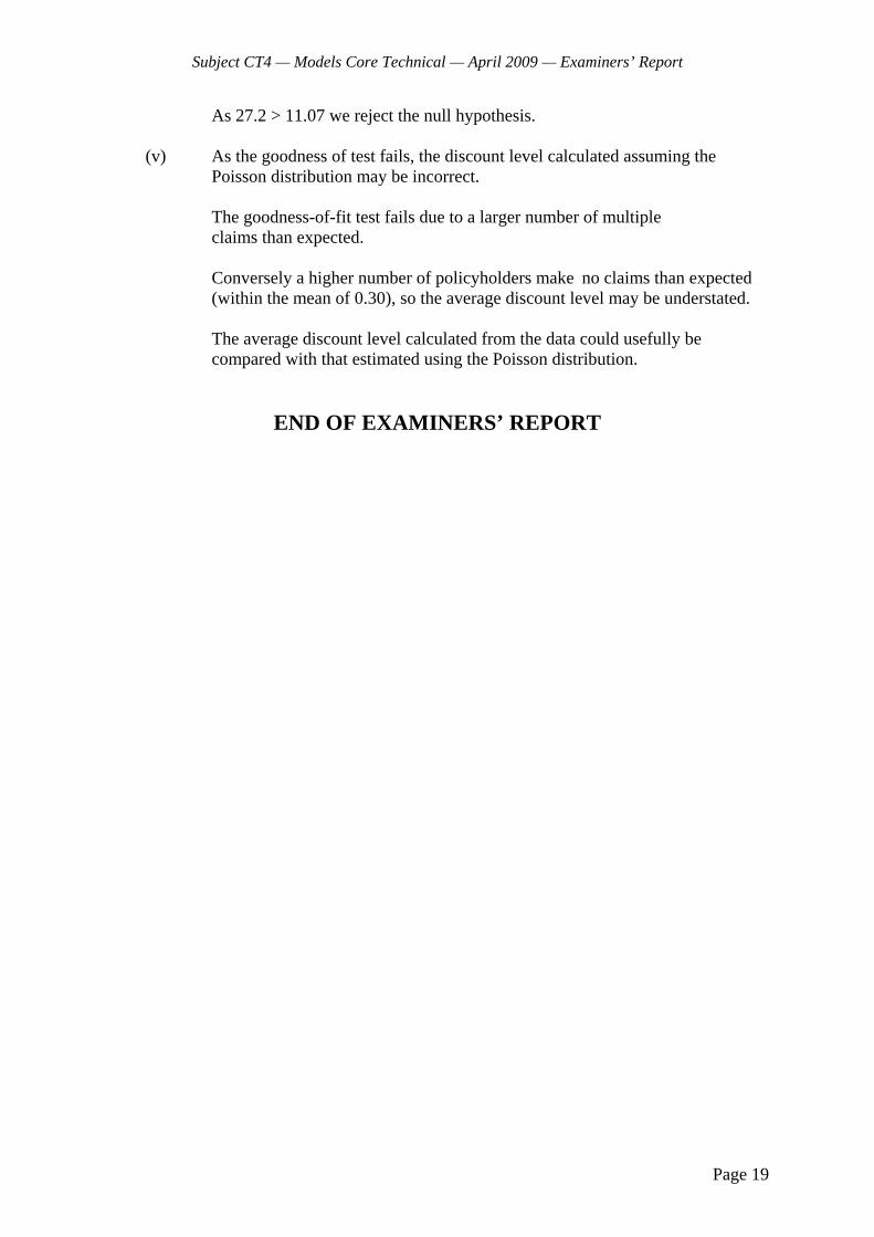
Subject CT4 — Models Core Technical — April 2009 — Examiners’ Report
Page 19
As 27.2 > 11.07 we reject the null hypothesis. (v) As the goodness of test fails, the discount level calculated assuming the
Poisson distribution may be incorrect.
The goodness-of-fit test fails due to a larger number of multiple claims than expected. Conversely a higher number of policyholders make no claims than expected
(within the mean of 0.30), so the average discount level may be understated.
The average discount level calculated from the data could usefully be compared with that estimated using the Poisson distribution.
END OF EXAMINERS’ REPORT

Faculty of Actuaries Institute of Actuaries
EXAMINATION
8 October 2009 (am)
Subject CT4 — Models Core Technical
Time allowed: Three hours
INSTRUCTIONS TO THE CANDIDATE
1. Enter all the candidate and examination details as requested on the front of your answer booklet.
2. You must not start writing your answers in the booklet until instructed to do so by the
supervisor. 3. Mark allocations are shown in brackets. 4. Attempt all 11 questions, beginning your answer to each question on a separate sheet. 5. Candidates should show calculations where this is appropriate.
Graph paper is not required for this paper.
AT THE END OF THE EXAMINATION
Hand in BOTH your answer booklet, with any additional sheets firmly attached, and this question paper.
In addition to this paper you should have available the 2002 edition of the Formulae and Tables and your own electronic calculator from the approved list.
© Faculty of Actuaries CT4 S2009 © Institute of Actuaries

CT4 S2009—2
1 Describe the difference between the following assumptions about mortality between any two ages, x and y (y > x):
• uniform distribution of deaths • constant force of mortality
In your answer, explain the shape of the survival function between ages x and y under
each of the two assumptions. [2] 2 (i) List the key steps in constructing a new actuarial model. [4] You work for an actuarial consultancy which is taking over responsibility for a
modelling process which has previously been conducted in house by a client. (ii) Discuss the extent to which the steps required for this task differ from those
listed in your answer to (i). [2] [Total 6] 3 (i) List the data needed for the exact calculation of a central exposed to risk
depending on age. [2] An investigation studied the mortality of persons aged between exact ages 40 and 41
years. The investigation began on 1 January 2008 and ended on 31 December 2008. The following table gives details of 10 lives involved in the investigation.
Life Date of 40th birthday Date of death
1 1 March 2007 – 2 1 May 2007 1 October 2008 3 1 July 2007 – 4 1 October 2007 – 5 1 December 2007 1 February 2008 6 1 February 2008 – 7 1 April 2008 – 8 1 June 2008 1 November 2008 9 1 August 2008 – 10 1 December 2008 –
Persons with no date of death given were still alive when the investigation ended.
(ii) Calculate a central exposed to risk using the data for the 10 lives in the sample. [3]
(iii) (a) Calculate the maximum likelihood estimate of the hazard of death at
age 40 last birthday. (b) Hence, or otherwise, estimate q40. [2] [Total 7]
CT4 S2009—3 PLEASE TURN OVER
4 (i) In the context of mortality investigations describe the principle of correspondence and give an example of a situation in which it may be hard to adhere to this principle. [2]
On 1 January 2005 a country introduced a comprehensive system of death
registration, which classified deaths by age last birthday on the date of death. The government of the country wishes to obtain estimates of the force of mortality,
xμ , by single years of age x for the period between 1 January 2005 and 1 January 2008. Annual population censuses have been taken on 30 June each year since 2004, which classify the population by age last birthday. However the only copy of the data from the population census of 30 June 2006 was lost when the computer disc on which it was stored was being transferred between government departments.
Let the population aged x last birthday on 30 June in year t be denoted by the symbol
,x tP , and the number of deaths during the period of investigation of persons aged x be denoted by the symbol dx.
(ii) Derive an expression in terms of ,x tP and dx which may be used to estimate
xμ . [6] [Total 8] 5 (i) State the Markov property. [1] A stochastic process X(t) operates with state space S. (ii) Prove that if the process has independent increments it satisfies the Markov
property. [3]
(iii) (a) Describe the difference between a Markov chain and a Markov jump process.
(b) Explain what is meant by a Markov chain being irreducible.
[2]
An actuarial student can see the office lift (elevator) from his desk. The lift has an indicator which displays on which of the office’s five floors it is at any point in time. For light relief the student decides to construct a model to predict the movements of the lift.
(iv) Explain whether it would be appropriate to select a model which is:
(a) irreducible (b) has the Markov property
[3] [Total 9]

CT4 S2009—4
6 The complaints department of a company has two employees, both of whom work five days per week.
The company models the arrival of complaints using a Poisson process with rate 1.25
per working day. (i) List the assumptions underlying the Poisson process model. [2] On receipt of a complaint, it is immediately assessed as being straightforward, of
medium difficulty or complicated. 60% of cases are assessed as straightforward and 10% are assessed as complicated. The time taken in person-days’ effort to prepare responses is assumed to follow an exponential distribution, with parameters 2 for straightforward complaints, 1 for medium difficulty complaints and 0.25 for complicated complaints.
(ii) Calculate the average number of person-days’ work expected to be generated
by complaints arriving during a five-day working week. [2] (iii) Define a state space under which the number of outstanding complaints can be
modelled as a Markov jump process. [2] The company has a service standard of responding to complaints within a fixed
number of days of receipt. It is considering using this Markov jump process to model the probability of failing to meet this service standard.
(iv) Discuss the appropriateness of using the model for this purpose, with reference
to the assumptions being made. [3] [Total 9] 7 A firm rents cars and operates from three locations — the Airport, the Beach and the
City. Customers may return vehicles to any of the three locations. The company estimates that the probability of a car being returned to each location is as follows:
Car returned to Car hired from
Airport Beach City
Airport 0.5 0.25 0.25 Beach 0.25 0.75 0 City 0.25 0.25 0.5
(i) Calculate the 2-step transition matrix. [2] (ii) Calculate the stationary distribution π . [3] It is suggested that the cars should be based at each location in proportion to the
stationary distribution. (iii) Comment on this suggestion. [2]
CT4 S2009—5 PLEASE TURN OVER
(iv) Sketch, using your answers to parts (i) and (ii), a graph showing the probability that a car currently located at the Airport is subsequently at the Airport, Beach or City against the number of times the car has been rented. [3]
[Total 10] 8 A researcher is studying a certain incurable disease. The disease can be fatal, but
often sufferers survive with the condition for a number of years. The researcher wishes to project the number of deaths caused by the disease by using a multiple state model with state space:
{H – Healthy, I – Infected, D(from disease) – Dead (caused by the disease), D(not from disease)
– Dead (not caused by the disease)}. The transition rates, dependent on age x, are as follows:
• a mortality rate from the Healthy state of ( )xμ • a rate of infection with the disease ( )xσ • a mortality rate from the Infected state of ( )xυ of which ( )xρ relates to Deaths
caused by the disease
(i) Draw a transition diagram for the multiple state model. [2] (ii) Write down Kolmogorov’s forward equations governing the transitions by
specifying the transition matrix. [3] (iii) Determine integral expressions, in terms of the transition rates and any
expressions previously determined, for:
(a) PHH(x, x + t) (b) PHI(x, x + t) (c) PHD(from disease)(x, x + t)
[5] [Total 10]

CT4 S2009—6
9 An electronics company developed a revolutionary new battery which it believed would make it enormous profits. It commissioned a sub-contractor to estimate the survival function of battery life for the first 12 prototypes. The sub-contractor inserted each prototype battery into an identical electrical device at the same time and measured the duration elapsing between the time each device was switched on and the time its battery ran out. The sub-contractor was instructed to terminate the test immediately after the failure of the 8th battery, and to return all 12 batteries to the company.
When the test was complete, the sub-contractor reported that he had terminated the
test after 150 days. He further reported that:
• two batteries had failed after 97 days • three further batteries had failed after 120 days • two further batteries had failed after 141 days • one further battery had failed after 150 days
However, he reported that he was only able to return 11 batteries, as one had exploded
after 110 days, and he had treated this battery as censored at that duration when working out the Kaplan-Meier estimate of the survival function.
(i) State, with reasons, the forms of censoring present in this study. [2] (ii) Calculate the Kaplan-Meier estimate of the survival function based on the
information supplied by the sub-contractor. [5] In his report, the sub-contractor claimed that the Kaplan-Meier estimate of the
survival function at the duration when the investigation was terminated was 0.2727. (iii) Explain why the sub-contractor’s Kaplan-Meier estimate would be consistent
with him having stolen the battery he claimed had exploded. [4] [Total 11]
CT4 S2009—7 PLEASE TURN OVER
10 An investigation into the mortality of men engaged in a hazardous occupation was carried out. The following is an extract from the results.
Age x Initial Observed ˆxq exposed-to-risk Ex deaths xθ 30 950 12 0.0126 31 1,200 14 0.0117 32 1,200 16 0.0133 33 900 9 0.0100 34 1,000 11 0.0110 35 1,100 15 0.0136 36 800 10 0.0125 37 1,250 16 0.0128 38 1,400 17 0.0121 It was decided to graduate the results with reference to English Life Table 15 (males).
The formula used for the graduation was 10o
sxxq q= .
(i) Using a test of the overall fit of the graduated rates to the data, test the
hypothesis that the underlying mortality of men in the hazardous occupation is in accordance with the graduation formula given above. [6]
(ii) Test the graduation using two other tests which detect different features of the
graduation. For each test you apply:
(a) State the feature of the graduation it is designed to detect. (b) Carry out the test. (c) State your conclusion. [7] [Total 13]

CT4 S2009—8
11 A study was undertaken into the length of spells of unemployment among young people in a certain city. A sample of young people was monitored from the time they started to claim unemployment benefit until either they resumed work, or they moved away from the city. None of the members of the sample died during the study.
The study investigated the impact of age, sex and educational qualifications on the
hazard of returning to work using the following covariates: A a young person’s age when he or she started claiming benefit (measured in
exact years since his or her 16th birthday)
S a dummy variable taking the value 1 if the person was male and 0 if the person was female
E a dummy variable taking the value 1 if the person had passed a school leaving examination in mathematics, and 0 otherwise
with associated parameters Aβ , Sβ and Eβ . The investigators decided to use a Cox proportional hazards regression model for the
study. (i) Explain what is meant by a proportional hazards model. [3] (ii) Explain why the Cox model is a popular model for the analysis of survival
data. [3] (iii) (a) Write down the equation of the model that was estimated, defining the terms you use (other than those defined above). (b) List the characteristics of the young person to whom the baseline hazard applies. [3] The results showed:
• The hazard of resuming work for males who started claiming benefit aged 17 years exact and who had passed the mathematics examination was 1.5 times the hazard for males who started claiming benefit aged 16 years exact but who had not passed the mathematics examination.
• Females who had passed the mathematics examination were twice as likely to take
up a new job as were males of the same age who had failed the mathematics examination.
• Females who started claiming benefit aged 20 years exact and who had passed the
mathematics examination were twice as likely to resume work as were males who started claiming benefit aged 16 years exact and who had also passed the mathematics examination.
(iv) Calculate the estimated values of the parameters Aβ , Sβ and Eβ . [6] [Total 15]
END OF PAPER
Faculty of Actuaries Institute of Actuaries
Faculty of Actuaries
Institute of Actuaries
Subject CT4 — Models.
Core Technical
September 2009 Examinations
EXAMINERS REPORT
Introduction
The attached subject report has been written by the Principal Examiner with the aim of
helping candidates. The questions and comments are based around Core Reading as the
interpretation of the syllabus to which the examiners are working. They have however given
credit for any alternative approach or interpretation which they consider to be reasonable.
R D Muckart
Chairman of the Board of Examiners
December 2009
Comments for individual questions are given with the solutions that follow.
Subject CT4 — Models Core Technical — September 2009 — Examiners’ Report
Page 2
Examiners’ Comments
Comments on solutions presented to individual questions for the September 2009 paper are
given below. In general, those using this report should be aware that in the case of non-
numerical answers full credit could often be obtained for rather less than is given in the
solutions which follow. The solutions are meant as a guide to the various points which could
have been made and considered relevant.
1
A uniform distribution of deaths means
EITHER
that deaths are evenly spaced between the ages x and y.
OR
that t x xq tq ( t y x )
OR
that t x x tp is constant for t y x .
It also means that the survival function decreases linearly between ages x and y. The
assumption of a constant force of mortality between any two ages means
EITHER
that the hazard does not change with age over this age range.
OR
that ( )t
t x xp p .
This implies that the survival function decreases exponentially between ages x and y.
Answers to this straightforward bookwork question were disappointing. Although
most candidates could describe the difference between a constant force of mortality
and the increasing force implied by a uniform distribution of deaths, few made correct
reference to the form of the survival function. An alarming number of candidates
referred to survival functions which increased with age! Credit was given for graphs
which correctly depicted the shape of the survival function under the two
assumptions.
2
(i) Define objectives of modelling process.
Plan the modelling process and how it will be validated.
Collect and validate the data required.

Subject CT4 — Models Core Technical — September 2009 — Examiners’ Report
Page 3
Define the form of the model.
Involve experts on the real world system/get feedback on validity.
Decide on software to be used, choose random number generator etc.
Write the computer program.
Debug the program.
Analyse the output
Test the reasonableness of the output.
Consider appropriateness of response of the model to small changes in input
parameters.
Communicate and document results.
[½ mark was awarded for each point up to a maximum of 4 marks]
(ii) Whilst in theory all steps are still required, some may take the form of
reviewing the appropriateness of existing decisions made, such as how the
form of the model was determined.
Extent of work will depend on whether the existing model is to be used,
adapted or superseded.
An understanding of how results compare with those previously used by the
company will be required.
Process maps for the existing approach, or discussions with the people running
the process about what they do, may be helpful.
The scope needs to be tightly defined up front to ensure it is clear what is
expected of the consultancy.
Data sources may already be established.
[½ mark was awarded for each point up to a maximum of 2 marks]
Part (i) of this question was basic bookwork and was extremely well
answered. Part (ii) required more thought, but many candidates were able to
write down some relevant points.
3
(i) For each life we need
EITHER date of birth OR exact age at entry into observation OR exact age at
exit from observation
Date of entry into observation
Date of exit from observation
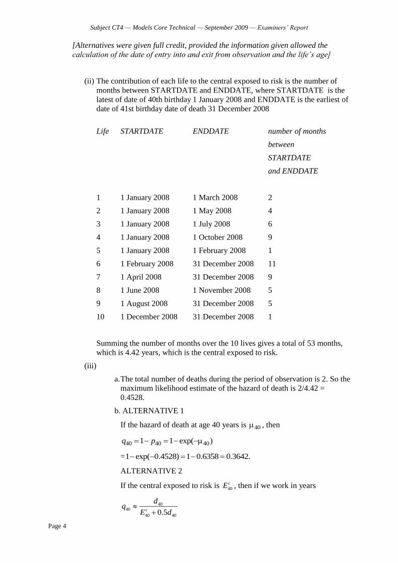
Subject CT4 — Models Core Technical — September 2009 — Examiners’ Report
Page 4
[Alternatives were given full credit, provided the information given allowed the
calculation of the date of entry into and exit from observation and the life’s age]
(ii) The contribution of each life to the central exposed to risk is the number of
months between STARTDATE and ENDDATE, where STARTDATE is the
latest of date of 40th birthday 1 January 2008 and ENDDATE is the earliest of
date of 41st birthday date of death 31 December 2008
Life STARTDATE ENDDATE number of months
between
STARTDATE
and ENDDATE
1 1 January 2008 1 March 2008 2
2 1 January 2008 1 May 2008 4
3 1 January 2008 1 July 2008 6
4 1 January 2008 1 October 2008 9
5 1 January 2008 1 February 2008 1
6 1 February 2008 31 December 2008 11
7 1 April 2008 31 December 2008 9
8 1 June 2008 1 November 2008 5
9 1 August 2008 31 December 2008 5
10 1 December 2008 31 December 2008 1
Summing the number of months over the 10 lives gives a total of 53 months,
which is 4.42 years, which is the central exposed to risk.
(iii)
a. The total number of deaths during the period of observation is 2. So the
maximum likelihood estimate of the hazard of death is 2/4.42 =
0.4528.
b. ALTERNATIVE 1
If the hazard of death at age 40 years is 40 , then
40 40 401 1 exp( )q p
=1 exp( 0.4528) 1 0.6358 0.3642.
ALTERNATIVE 2
If the central exposed to risk is 40
cE , then if we work in years
4040
40 400.5c
dq
E d
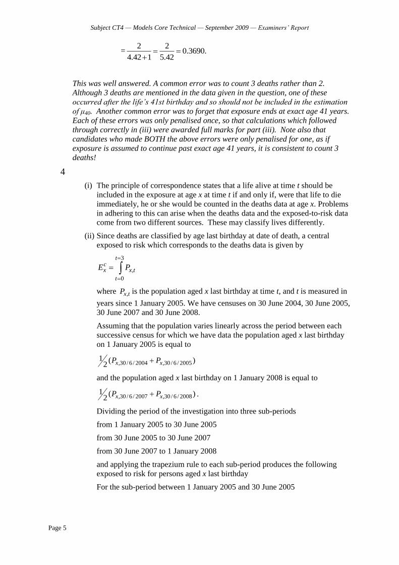
Subject CT4 — Models Core Technical — September 2009 — Examiners’ Report
Page 5
=2 2
0.3690.4.42 1 5.42
This was well answered. A common error was to count 3 deaths rather than 2.
Although 3 deaths are mentioned in the data given in the question, one of these
occurred after the life’s 41st birthday and so should not be included in the estimation
of μ40. Another common error was to forget that exposure ends at exact age 41 years.
Each of these errors was only penalised once, so that calculations which followed
through correctly in (iii) were awarded full marks for part (iii). Note also that
candidates who made BOTH the above errors were only penalised for one, as if
exposure is assumed to continue past exact age 41 years, it is consistent to count 3
deaths!
4
(i) The principle of correspondence states that a life alive at time t should be
included in the exposure at age x at time t if and only if, were that life to die
immediately, he or she would be counted in the deaths data at age x. Problems
in adhering to this can arise when the deaths data and the exposed-to-risk data
come from two different sources. These may classify lives differently.
(ii) Since deaths are classified by age last birthday at date of death, a central
exposed to risk which corresponds to the deaths data is given by
3
,
0
tcx x t
t
E P
where ,x tP is the population aged x last birthday at time t, and t is measured in
years since 1 January 2005. We have censuses on 30 June 2004, 30 June 2005,
30 June 2007 and 30 June 2008.
Assuming that the population varies linearly across the period between each
successive census for which we have data the population aged x last birthday
on 1 January 2005 is equal to
,30 / 6 / 2004 ,30 / 6 / 20051 ( )
2 x xP P
and the population aged x last birthday on 1 January 2008 is equal to
,30 / 6 / 2007 ,30 / 6 / 20081 ( )
2 x xP P .
Dividing the period of the investigation into three sub-periods
from 1 January 2005 to 30 June 2005
from 30 June 2005 to 30 June 2007
from 30 June 2007 to 1 January 2008
and applying the trapezium rule to each sub-period produces the following
exposed to risk for persons aged x last birthday
For the sub-period between 1 January 2005 and 30 June 2005
Subject CT4 — Models Core Technical — September 2009 — Examiners’ Report
Page 6
,1/1/2005 ,30/6/2005
,30/6/2004 ,30/6/2005 ,30/6/2005
1 1 ( )2 2
1 1 1( ( ) )2 2 2
x x
x x x
P P
P P P
For the sub-period between 30 June 2005 and 30 June 2007
,30/6/2005 ,30/6/200712 ( )
2 x xP P
For the sub-period between 30 June 2007 and 1 January 2008
,30/6/2007 ,1/1/2008
,30/6/2007 ,30/6/2007 ,30/6/2008
1 1 ( )2 2
1 1 1( ( ))2 2 2
x x
x x x
P P
P P P
Summing these gives
,30/6/2004 ,30/6/2005 ,30/6/2005 ,30/6/2005
,30/6/2007 ,30/6/2007 ,30/6/2007 ,30/6/2008
1 1 18 8 4
1 1 14 8 8
cx x x x x
x x x x
E P P P P
P P P P
which simplifies to
,30/6/2004 ,30/6/2005 ,30/6/2007 ,30/6/20081 11 11 1
8 8 8 8cx x x x xE P P P P .
The force of mortality may be estimated using the formula
xx c
x
d
E ,
where xd denotes deaths to persons aged x last birthday when they died.
This was very poorly answered. It was perhaps rather more difficult than some
exposed-to-risk questions in previous examination papers, but nevertheless the
standard of most attempts was disappointing. In part (ii) credit was given for various
alternative approximations provided that they were explained clearly.
5
(i) The Markov property states that the future development of a process can be
predicted from its present state alone without reference to its past history.
(ii) Formally, for times 1 2 ... ns s s s t and for states 1 2, ,..., ,nx x x x in the
state space S and all subsets A of S, the Markov property can be written
1 1 2 2Pr[ ( ) | ( ) , ( ) ,...., ( ) , ( ) ] Pr[ | ( ) ]n n tX t A X s x X s x X s x X s x X A X s x
For independent increments we can write
1 1 2 2
1 1 2 2
Pr[ ( ) | ( ) , ( ) ,...., ( ) , ( ) ]
Pr[ ( ) ( ) | ( ) , ( ) ,...., ( ) , ( ) ]
Pr[ ( ) ( ) | ( ) ]
Pr[ ( ) | ( ) ]
n n
n n
X t A X s x X s x X s x X s x
X t X s x A X s x X s x X s x X s x
X t X s x A X s x
X t A X s x

Subject CT4 — Models Core Technical — September 2009 — Examiners’ Report
Page 7
(iii)
a. A Markov chain is a stochastic process with the Markov property
which has a discrete time set with a discrete state space. A Markov
jump process is a stochastic process with the Markov property which
has a continuous time set with a discrete state space.
b.A Markov chain is irreducible if any state can be reached from any
other state.
(iv)
a. A lift could not serve its purpose unless it could return to each of the
floors which it serves. This means an irreducible model would be
appropriate.
b.Suppose, for example, the lift is currently at the third floor, with its last
two states being the fourth floor and the fifth floor. In such a case the
lift is more likely to be heading downwards than upwards. So the past
history is likely to provide information on the likely future movement
of the lift, unless the state space is very complicated (involving a
number of past floors as well as the current floor). Therefore a Markov
model is unlikely to be appropriate.
This question was generally well answered, apart from section (iv)(b) in which few
candidates spotted the point that the direction of travel of the lift as well as its current
floor will influence its next location.
6
(i) A Poisson process is a continuous-time integer valued process
Nt, 0t with
N0 = 0
independent increments
EITHER
increments follow a Poisson distribution
OR
[ ( )] exp[ ( )]
[ ]!
n
t s
t s t sP N N n
n
, for s < t, n = 0, 1, 2, ....
(ii) Average work created by a complaint is
60%* ½+ 30%* 1 + 10%*4 = 1 day.
Complaints arrive at a rate 1.25 per working day
So, work expected to be generated is 1.25*1*5 = 6.25 person-days.
(iii)As the time to handle complaints follows an exponential (memoryless)
distribution, only need to know how many unanswered complaints there are –

Subject CT4 — Models Core Technical — September 2009 — Examiners’ Report
Page 8
but do need to know how many of each type. If cases are allocated randomly
rather than in order, then the state space consists of (in terms of complaints not
resolved):
r – straightforward,
s – medium,
t – complicated.
where r = 0,1,2,3,4,5,….
s = 0,1,2,3,4,5,……
t = 0,1,2,3,4,5,…..
(iv) EITHER The model will only give an approximation.
OR The model is not suitable for this purpose.
The model could not be used to do this without extending the state space to
consider the time the complaint has been in the queue. There are only two
employees, so holidays and sickness are important factors not taken into
account.
The model assumes complaints are time-homogeneous. We do not know the
nature of the business, but for some industries complaints would be seasonal
e.g. holiday companies.
The model assumes that complaint arrivals are independent, but more
complaints might be expected if the company has had a quality control
problem at a particular time. If struggling to meet the service standard, action
would be. Taken, such as overtime, or prioritising easy cases. Staff may be
able to deal with complaints which are similar to other recent complaints very
quickly, using standard „template‟ responses.
The memoryless property is unlikely to be realistic as the work required to
complete the case could be assessed and then worked through to a schedule.
The Markov jump process could be used to estimate the probability that a
complaint is responded to within a given number of days of receipt.
So the model could be used to estimate the probability of a complaint not
being responded to in the stated time, that is the failure to meet the service
standard.
[½ mark was awarded for each point up to a maximum of 3 marks]
Answers to this question were disappointing. Most candidates were able to tackle the
calculation in part (ii) but few correctly identified the state space in part (iii), and
most only made a cursory attempt at part (iv).
7
(i) Two step transition matrix
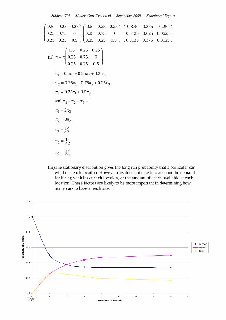
Subject CT4 — Models Core Technical — September 2009 — Examiners’ Report
Page 9
=
0.5 0.25 0.25
0.25 0.75 0
0.25 0.25 0.5
.
0.5 0.25 0.25
0.25 0.75 0
0.25 0.25 0.5
=
0.375 0.375 0.25
0.3125 0.625 0.0625
0.3125 0.375 0.3125
(ii)
0.5 0.25 0.25
0.25 0.75 0
0.25 0.25 0.5
1 1 2 30.5 0.25 0.25
2 1 2 30.25 0.75 0.25
3 1 30.25 0.5
and 1 2 3 1
1 32
2 33
11
3
21
2
31
6
(iii)The stationary distribution gives the long run probability that a particular car
will be at each location. However this does not take into account the demand
for hiring vehicles at each location, or the amount of space available at each
location. These factors are likely to be more important in determining how
many cars to base at each site.
0
0.2
0.4
0.6
0.8
1
1.2
0 1 2 3 4 5 6 7 8 9
Number of rentals
Pro
bab
ilty
at lo
cati
on
Airport
Beach
City
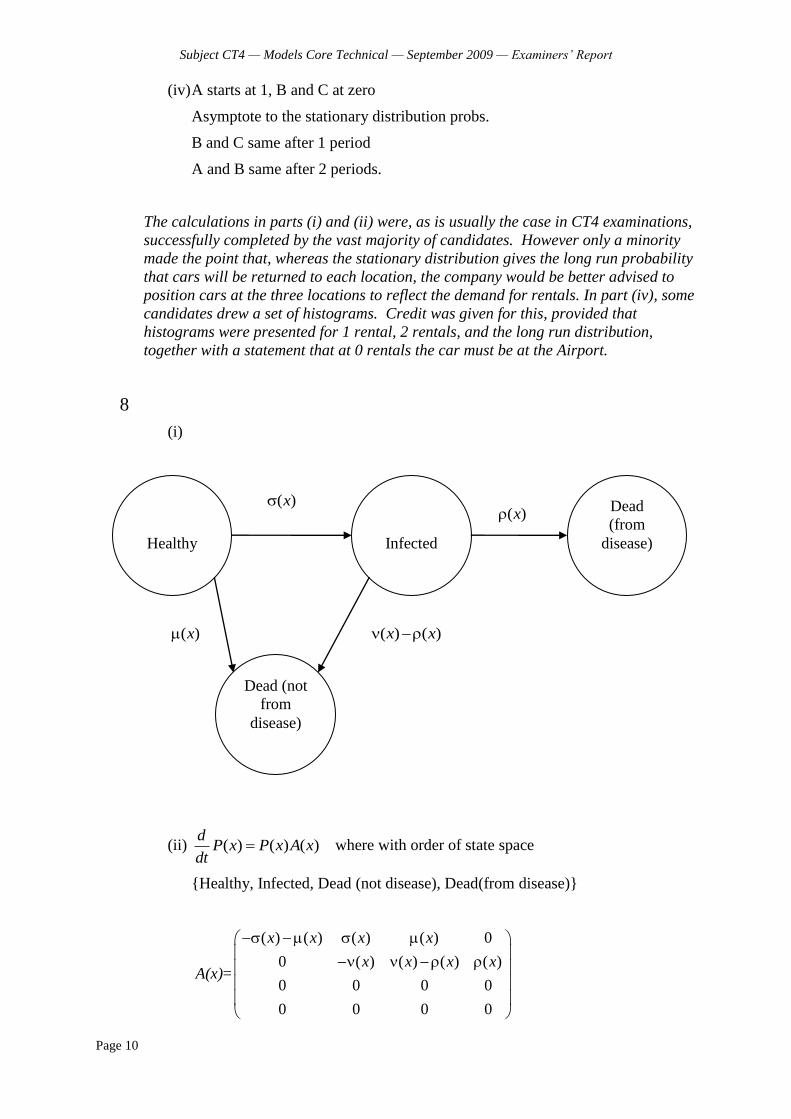
Subject CT4 — Models Core Technical — September 2009 — Examiners’ Report
Page 10
(iv) A starts at 1, B and C at zero
Asymptote to the stationary distribution probs.
B and C same after 1 period
A and B same after 2 periods.
The calculations in parts (i) and (ii) were, as is usually the case in CT4 examinations,
successfully completed by the vast majority of candidates. However only a minority
made the point that, whereas the stationary distribution gives the long run probability
that cars will be returned to each location, the company would be better advised to
position cars at the three locations to reflect the demand for rentals. In part (iv), some
candidates drew a set of histograms. Credit was given for this, provided that
histograms were presented for 1 rental, 2 rentals, and the long run distribution,
together with a statement that at 0 rentals the car must be at the Airport.
8
(i)
(ii) ( ) ( ) ( )d
P x P x A xdt
where with order of state space
{Healthy, Infected, Dead (not disease), Dead(from disease)}
A(x)=
( ) ( ) ( ) ( ) 0
0 ( ) ( ) ( ) ( )
0 0 0 0
0 0 0 0
x x x x
x x x x
Healthy
Infected
Dead
(from
disease)
Dead (not
from
disease)
( )x ( )x
( )x ( ) ( )x x
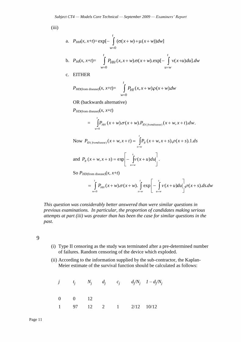
Subject CT4 — Models Core Technical — September 2009 — Examiners’ Report
Page 11
(iii)
a. PHH(x, x+t)=
0
exp[ ( ( ) ( )) ]
t
w
x w x w dw
b. PHI(x, x+t)=
0
( , ). ( ).exp[ ( ) ].
t t
HH
w u w
P x x w x w x u du dw
c. EITHER
PHD(from disease)(x, x+t)=
0
( , ). ( ).
t
HI
w
P x x w x w dw
OR (backwards alternative)
PHD(from disease)(x, x+t)
=
t
w
efromdiseasIDHH dwtxwxPwxwxP0
)( ).,().().( .
Now dssxsxwxPtxwxP
t
ws
IIefromdiseasID .1).().,(),()(
and
s
wu
II duuxsxwxP )(exp),( .
So PHD(from disease)(x, x+t)
0
( ). ( ). exp ( ) . ( ). .
t t s
HH
w s w u w
P x w x w x u du x s ds dw
This question was considerably better answered than were similar questions in
previous examinations. In particular, the proportion of candidates making serious
attempts at part (iii) was greater than has been the case for similar questions in the
past.
9
(i) Type II censoring as the study was terminated after a pre-determined number
of failures. Random censoring of the device which exploded.
(ii) According to the information supplied by the sub-contractor, the Kaplan-
Meier estimate of the survival function should be calculated as follows:
j tj Nj dj cj dj/Nj 1 – dj/Nj
0 0 12
1 97 12 2 1 2/12 10/12
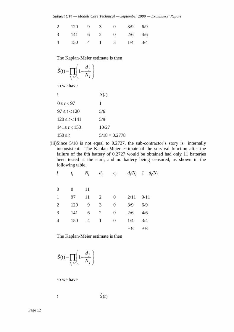
Subject CT4 — Models Core Technical — September 2009 — Examiners’ Report
Page 12
2 120 9 3 0 3/9 6/9
3 141 6 2 0 2/6 4/6
4 150 4 1 3 1/4 3/4
The Kaplan-Meier estimate is then
ˆ( ) 1
j
j
jt t
dS t
N
so we have
t ˆ( )S t
0 97t 1
97 120t 5/6
120 141t 5/9
141 150t 10/27
150 t 5/18 = 0.2778
(iii)Since 5/18 is not equal to 0.2727, the sub-contractor‟s story is internally
inconsistent. The Kaplan-Meier estimate of the survival function after the
failure of the 8th battery of 0.2727 would be obtained had only 11 batteries
been tested at the start, and no battery being censored, as shown in the
following table.
j tj Nj dj cj dj/Nj 1 – dj/Nj
0 0 11
1 97 11 2 0 2/11 9/11
2 120 9 3 0 3/9 6/9
3 141 6 2 0 2/6 4/6
4 150 4 1 0 1/4 3/4
+½ +½
The Kaplan-Meier estimate is then
ˆ( ) 1
j
j
jt t
dS t
N
so we have
t ˆ( )S t
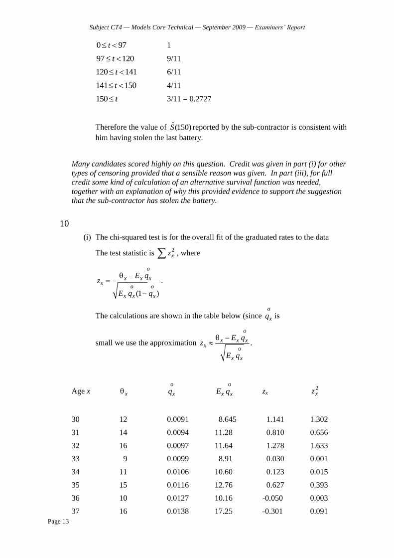
Subject CT4 — Models Core Technical — September 2009 — Examiners’ Report
Page 13
0 97t 1
97 120t 9/11
120 141t 6/11
141 150t 4/11
150 t 3/11 = 0.2727
Therefore the value of ˆ(150)S reported by the sub-contractor is consistent with
him having stolen the last battery.
Many candidates scored highly on this question. Credit was given in part (i) for other
types of censoring provided that a sensible reason was given. In part (iii), for full
credit some kind of calculation of an alternative survival function was needed,
together with an explanation of why this provided evidence to support the suggestion
that the sub-contractor has stolen the battery.
10
(i) The chi-squared test is for the overall fit of the graduated rates to the data
The test statistic is 2xz , where
(1 )
o
x x xx
o o
x x x
E qz
E q q
.
The calculations are shown in the table below (since o
xq is
small we use the approximation
o
x x xx
o
x x
E qz
E q
.
Age x x o
xq o
x xE q zx 2xz
30 12 0.0091 8.645 1.141 1.302
31 14 0.0094 11.28 0.810 0.656
32 16 0.0097 11.64 1.278 1.633
33 9 0.0099 8.91 0.030 0.001
34 11 0.0106 10.60 0.123 0.015
35 15 0.0116 12.76 0.627 0.393
36 10 0.0127 10.16 -0.050 0.003
37 16 0.0138 17.25 -0.301 0.091

Subject CT4 — Models Core Technical — September 2009 — Examiners’ Report
Page 14
38 17 0.0149 20.86 -0.845 0.714
∑ 4.808
The test statistic has a chi-squared distribution with degrees of freedom (d.f.)
given by number of ages
– 1 (for parameter of function linking o
xq and sxq )
– some d.f. for constraints imposed by choice of standard table
The critical value of the chi-squared distribution is
11.07 with 5 d.f.
12.59 with 6 d.f.
14.07 with 7 d.f.
15.51 with 8 d.f.
16.92 with 9 d.f. at the 5% level (from tables)
Since 4.808 < 11.07 (or 12.59 etc.) there is no evidence to reject the null
hypothesis that the graduated rates are the true rates underlying the crude
rates.
(ii) EITHER
Signs test
a. The Signs test looks for overall bias.
b. The number of positive signs among the xz s
is distributed Binomial (9, 0.5).
We observe 6 positive signs.
The probability of obtaining 6 or more positive signs is
(from tables)
1 – 0.7461 = 0.2539.
[Alternatively, candidates could calculate the probability of obtaining exactly 6
positive signs, which is 0.1641]
Since this is greater than 0.025 (two-tailed test)
c. we cannot reject the null hypothesis and we conclude that the
graduated rates are not systematically higher or lower than the crude
rates.
OR
Cumulative Deviations test
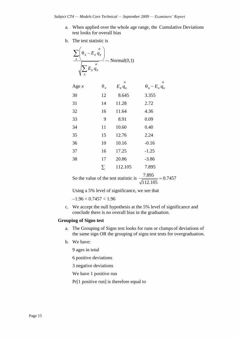
Subject CT4 — Models Core Technical — September 2009 — Examiners’ Report
Page 15
a. When applied over the whole age range, the Cumulative Deviations
test looks for overall bias
b. The test statistic is
Normal(0,1)
o
x x x
x
o
x x
x
E q
E q
Age x x o
x xE q o
x x xE q
30 12 8.645 3.355
31 14 11.28 2.72
32 16 11.64 4.36
33 9 8.91 0.09
34 11 10.60 0.40
35 15 12.76 2.24
36 10 10.16 -0.16
37 16 17.25 -1.25
38 17 20.86 -3.86
∑ 112.105 7.895
So the value of the test statistic is 7.895
0.7457112.105
Using a 5% level of significance, we see that
1.96 < 0.7457 < 1.96
c. We accept the null hypothesis at the 5% level of significance and
conclude there is no overall bias in the graduation.
Grouping of Signs test
a. The Grouping of Signs test looks for runs or clumps of deviations of
the same sign OR the grouping of signs test tests for overgraduation.
b. We have:
9 ages in total
6 positive deviations
3 negative deviations
We have 1 positive run
Pr[1 positive run] is therefore equal to
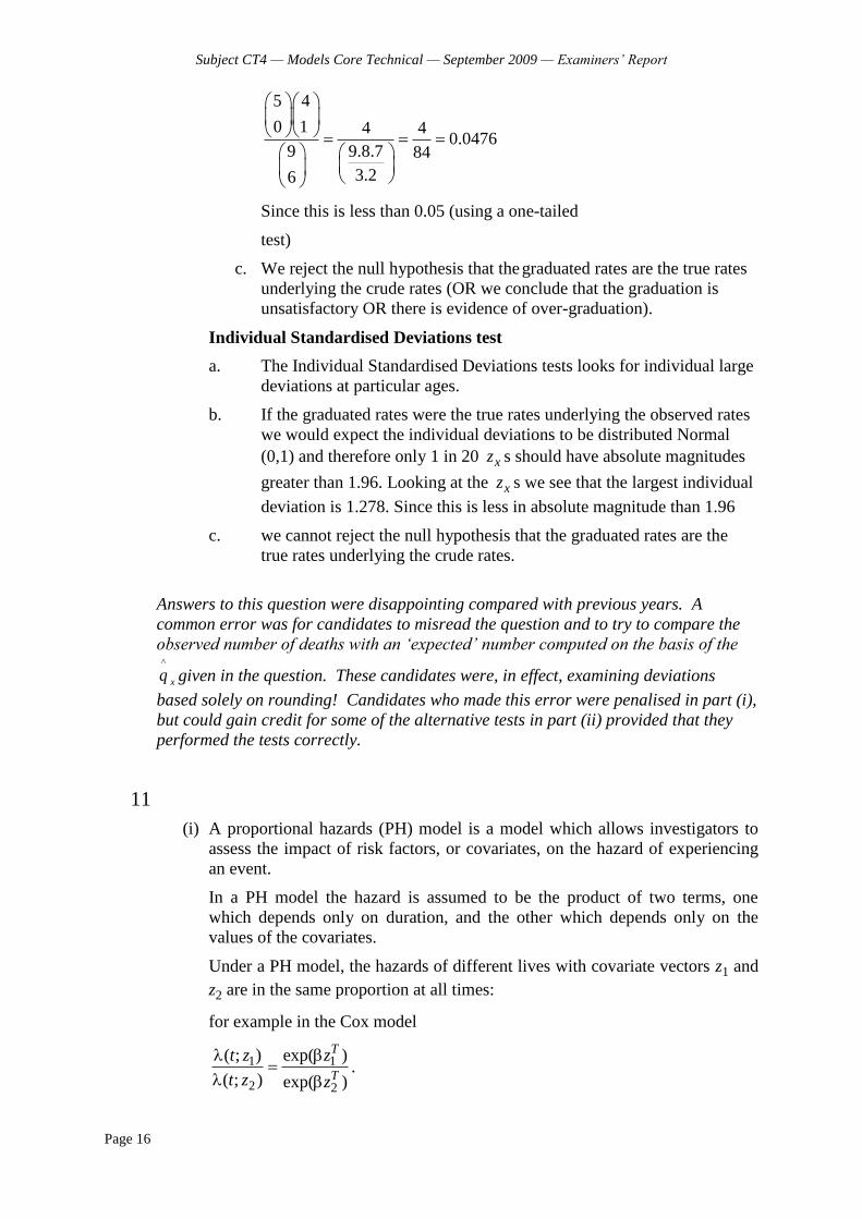
Subject CT4 — Models Core Technical — September 2009 — Examiners’ Report
Page 16
5 4
0 1 4 40.0476
9 9.8.7 84
3.26
Since this is less than 0.05 (using a one-tailed
test)
c. We reject the null hypothesis that the graduated rates are the true rates
underlying the crude rates (OR we conclude that the graduation is
unsatisfactory OR there is evidence of over-graduation).
Individual Standardised Deviations test
a. The Individual Standardised Deviations tests looks for individual large
deviations at particular ages.
b. If the graduated rates were the true rates underlying the observed rates
we would expect the individual deviations to be distributed Normal
(0,1) and therefore only 1 in 20 xz s should have absolute magnitudes
greater than 1.96. Looking at the xz s we see that the largest individual
deviation is 1.278. Since this is less in absolute magnitude than 1.96
c. we cannot reject the null hypothesis that the graduated rates are the
true rates underlying the crude rates.
Answers to this question were disappointing compared with previous years. A
common error was for candidates to misread the question and to try to compare the
observed number of deaths with an ‘expected’ number computed on the basis of the
xq^
given in the question. These candidates were, in effect, examining deviations
based solely on rounding! Candidates who made this error were penalised in part (i),
but could gain credit for some of the alternative tests in part (ii) provided that they
performed the tests correctly.
11
(i) A proportional hazards (PH) model is a model which allows investigators to
assess the impact of risk factors, or covariates, on the hazard of experiencing
an event.
In a PH model the hazard is assumed to be the product of two terms, one
which depends only on duration, and the other which depends only on the
values of the covariates.
Under a PH model, the hazards of different lives with covariate vectors z1 and
z2 are in the same proportion at all times:
for example in the Cox model
1 1
2 2
( ; ) exp( )
( ; ) exp( )
T
T
t z z
t z z
.

Subject CT4 — Models Core Technical — September 2009 — Examiners’ Report
Page 17
(ii) Cox‟s model ensures that the hazard is always positive. Standard software
packages often include Cox‟s model.
Cox‟s model allows the general “shape” of the hazard function for all
individuals to be determined by the data, giving a high degree of flexibility
while an exponential term accounts for differences between individuals.
This means that if we are not primarily concerned with the precise form of the
hazard, we can ignore the shape of the baseline hazard and estimate the effects
of the covariates from the data directly.
(iii)
a. 0( ) ( )exp( )A E St t A E S , where ( )t is the estimated
hazard and 0 ( )t is the baseline hazard.
b. A female aged exactly 16 years when she first claimed benefit who had
not passed the school mathematics examination.
(iv) “The hazard of resuming work for males aged 17 years who had passed the
mathematics examination was 1.5 times the hazard for males aged 16 years
who had not passed the mathematics examination” implies that
exp[( *1) ]exp( )
exp( )
exp( )exp( ) 1.5
A S EA E
S
A E
“Females who had passed the examination were twice as likely to take up a
new job as were males of the same age who had failed” implies that
exp( )
2exp( )
E
S
since the age terms cancel out.
“Females aged 20 years who had passed the examination were twice as likely
to resume work as were males aged 16 years who had also passed the
examination” implies that
exp( *4)
2exp( )
A
S
.
Substituting from (2) into (1) gives
2exp( )exp( ) 1.5A S
so
exp( ) 0.75exp( )S A .
Substituting into (3) gives
exp[ *4)2
0.75exp( )
A
A
,
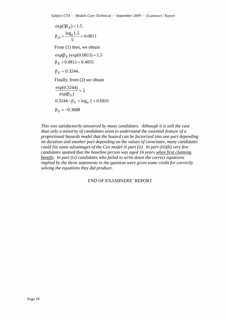
Subject CT4 — Models Core Technical — September 2009 — Examiners’ Report
Page 18
exp(5 ) 1.5
log 1.50.0811
5
A
eA
From (1) then, we obtain
exp( )exp(0.0811) 1.5
0.0811 0.4055
E
E
0.3244E .
Finally, from (2) we obtain
exp(0.3244)2
exp( )
0.3244 log 2 0.6931
S
S e
0.3688S
This was satisfactorily answered by many candidates. Although it is still the case
than only a minority of candidates seem to understand the essential feature of a
proportional hazards model that the hazard can be factorised into one part depending
on duration and another part depending on the values of covariates, many candidates
could list some advantages of the Cox model in part (ii). In part (iii)(b) very few
candidates spotted that the baseline person was aged 16 years when first claiming
benefit. In part (iv) candidates who failed to write down the correct equations
implied by the three statements in the question were given some credit for correctly
solving the equations they did produce.
END OF EXAMINERS‟ REPORT

Faculty of Actuaries Institute of Actuaries
EXAMINATION
21 April 2010 (am)
Subject CT4 — Models Core Technical
Time allowed: Three hours
INSTRUCTIONS TO THE CANDIDATE
1. Enter all the candidate and examination details as requested on the front of your answer booklet.
2. You must not start writing your answers in the booklet until instructed to do so by the
supervisor. 3. Mark allocations are shown in brackets. 4. Attempt all 12 questions, beginning your answer to each question on a separate sheet. 5. Candidates should show calculations where this is appropriate.
Graph paper is NOT required for this paper.
AT THE END OF THE EXAMINATION
Hand in BOTH your answer booklet, with any additional sheets firmly attached, and this question paper.
In addition to this paper you should have available the 2002 edition of the Formulae and Tables and your own electronic calculator from the approved list.
© Faculty of Actuaries CT4 A2010 © Institute of Actuaries
CT4 A2010—2
1 List four factors often used to subdivide life insurance mortality statistics. [2] 2 Write down integral equations for the mean and variance of the complete future
lifetime at age x, xT . [2] 3 For each of the following processes:
counting process; general random walk; compound Poisson process; Poisson process; Markov jump chain.
(a) State whether the state space is discrete, continuous or can be either. (b) State whether the time set is discrete, continuous, or can be either.
[5] 4 A Markov Chain with state space {A, B, C} has the following properties:
• it is irreducible
• it is periodic
• the probability of moving from A to B equals the probability of moving from A to C
(i) Show that these properties uniquely define the process. [4] (ii) Sketch a transition diagram for the process. [1]
[Total 5]

CT4 A2010—3 PLEASE TURN OVER
5 Ten years ago, a confectionery manufacturer launched a new product, the Scrummy Bar. The product has been successful, with a rapid increase in consumption since the product was first sold. In order to plan future investment in production capacity, the manufacturer wishes to forecast the future demand for Scrummy Bars. It has data on age-specific consumption rates for the past ten years, together with projections of the population by age over the next twenty years. It proposes the following modelling strategy:
• extrapolate past age-specific consumption rates to forecast age-specific
consumption rates for the next 20 years
• apply the forecast age-specific consumption rates to the projected population by age to obtain estimated total consumption of the product by age for each of the next 20 years
• sum the results to obtain the total demand for each year
Describe the advantages and disadvantages of this strategy. [5] 6 An oil company has discovered a vast deposit of oil in an equatorial swamp.
The area is extremely unhealthy and inhabited by venomous spiders. There is an antidote to bites from these spiders but it is expensive. The antidote acts instantly but does not provide future immunity. The company commissions a study to estimate the rate of being bitten by the spiders among its employees, in order to determine the amount of antidote to provide. Employees of the company are posted to the swamp for six month tours of duty starting on 1 January, 1 April, 1 July or 1 October. The first employees to be posted arrived on 1 January 2008. The swamp is so inaccessible that no employees are allowed to leave before their six month tours of duty are completed.
Accidental deaths are common in this dangerous location. The table below gives some data from the study. Quarter Number of new Number of Number of beginning arrivals at start accidental deaths spider bites of quarter during quarter during quarter 1 January 2008 90 10 15 1 April 2008 80 8 25 1 July 2008 114 10 30 1 October 2008 126 13 40 (i) Estimate the quarterly rate of being bitten by a spider for each quarter of
2008, stating any assumptions you make. [7] (ii) Suggest reasons why the assumptions you made in (i) might not be valid. [1]
[Total 8]
CT4 A2010—4
7 A government has introduced a two-tier driving test system. Once someone applies for a provisional licence they are considered a Learner driver. Learner drivers who score 90% or more on the primary examination (which can be taken at any time) become Qualified. Those who score between 50% and 90% are obliged to sit a secondary examination and are given driving status Restricted. Those who score 50% or below on the primary examination remain as Learners. Restricted drivers who pass the secondary examination become Qualified, but those who fail revert back to Learner status and are obliged to start again.
(i) Sketch a diagram showing the possible transitions between the states. [2] (ii) Write down the likelihood of the data, assuming transition rates between states
are constant over time, clearly defining all terms you use. [3]
Figures over the first year of the new system based on those who applied for a provisional licence during that time in one area showed the following:
Person-months in Learner State Person-months in Restricted State Number of transitions from Learner to Restricted Number of transitions from Restricted to Learner Number of transitions from Restricted to Qualified Number of transitions from Learner to Qualified
1,161 1,940 382 230 110 217
(iii) (a) Derive the maximum likelihood estimator of the transition rate from
Restricted to Learner. (b) Estimate the constant transition rate from Restricted to Learner. [3]
[Total 8]
CT4 A2010—5 PLEASE TURN OVER
8 A certain profession admits new members to the status of student. Students may qualify as fellows of the profession by virtue of passing a series of examinations. Normally student members sit the examinations whilst working for an employer. There are two sessions of the examinations each year.
An employer provides study support to student members of the profession. It wishes to assess the cost of providing this study support and therefore wishes to know the average time it can expect to take for its students to qualify. The employer has maintained records for 23 of its students who all sat their first examination in the first session of 2003. The students’ progress has been recorded up to and including the last session of 2009. The following data records the number of sessions which had been held before the specified event occurred for a student in this cohort: Qualified 6, 8, 8, 9, 9, 9, 11, 11, 13, 13, 13 Stopped studying 4, 5, 8, 11, 14
The remaining seven students were still studying for the examinations at the end of 2009.
(i) Determine the median number of sessions taken to qualify for those students who qualified during the period of observation. [2]
(ii) Calculate the Kaplan-Meier estimate of the survival function, S(t), for the
“hazard” of qualifying, where t is the number of sessions of examinations since 1 January 2003. [5]
(iii) Hence estimate the median number of sessions to qualify for the students of
this employer. [2] (iv) Explain the difference between the results in (i) and (iii) above. [2] [Total 11]
CT4 A2010—6
9 (i) Write down the hazard function for the Cox proportional hazards model defining all the terms that you use. [2] A farmer is concerned that he is losing a lot of his birds to a predator, so he decides to
build a new enclosure using taller fencing. This fencing is expensive and he cannot afford to build a large enough area for all his birds. He therefore decides to put half his birds in the new enclosure and leave the others in the existing enclosure. He is convinced that the new enclosure is an improvement, but has asked an actuarial student to determine whether the new enclosure will result in an increase in the life expectancy of his birds. The student has fitted a Cox proportional hazards model to data on the duration until a bird is killed by a predator and calculated the following figures relating to the regression parameters:
Bird Enclosure Sex
Chicken Duck Goose New Old Male Female
Parameter estimate 0
–0.210 0.075
0.125
0
0.2 0
Variance 0
0.002 0.004
0.0015
0
0.0026 0
(ii) State the features of the bird to which the baseline hazard applies. [1] (iii) For each regression parameter: (a) Define the associated covariate. (b) Calculate the 95% confidence interval based on the standard error. [3] (iv) Comment on the farmer’s belief that the new enclosure will result in an
increase in his birds’ life expectancy. [2] (v) Calculate, using this model, the probability that a female duck in the new
enclosure has been killed by a predator at the end of six months, given that the probability that a male goose in the old enclosure has been killed at the end of the same period is 0.1 (all other decrements can be ignored). [4]
[Total 12]
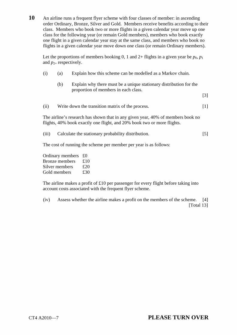
CT4 A2010—7 PLEASE TURN OVER
10 An airline runs a frequent flyer scheme with four classes of member: in ascending order Ordinary, Bronze, Silver and Gold. Members receive benefits according to their class. Members who book two or more flights in a given calendar year move up one class for the following year (or remain Gold members), members who book exactly one flight in a given calendar year stay at the same class, and members who book no flights in a given calendar year move down one class (or remain Ordinary members).
Let the proportions of members booking 0, 1 and 2+ flights in a given year be p0, p1
and p2+ respectively.
(i) (a) Explain how this scheme can be modelled as a Markov chain. (b) Explain why there must be a unique stationary distribution for the
proportion of members in each class. [3]
(ii) Write down the transition matrix of the process. [1]
The airline’s research has shown that in any given year, 40% of members book no flights, 40% book exactly one flight, and 20% book two or more flights.
(iii) Calculate the stationary probability distribution. [5] The cost of running the scheme per member per year is as follows: Ordinary members £0 Bronze members £10 Silver members £20 Gold members £30
The airline makes a profit of £10 per passenger for every flight before taking into account costs associated with the frequent flyer scheme.
(iv) Assess whether the airline makes a profit on the members of the scheme. [4] [Total 13]
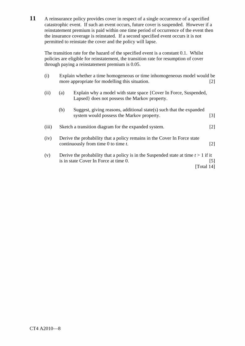
CT4 A2010—8
11 A reinsurance policy provides cover in respect of a single occurrence of a specified catastrophic event. If such an event occurs, future cover is suspended. However if a reinstatement premium is paid within one time period of occurrence of the event then the insurance coverage is reinstated. If a second specified event occurs it is not permitted to reinstate the cover and the policy will lapse.
The transition rate for the hazard of the specified event is a constant 0.1. Whilst
policies are eligible for reinstatement, the transition rate for resumption of cover through paying a reinstatement premium is 0.05.
(i) Explain whether a time homogeneous or time inhomogeneous model would be
more appropriate for modelling this situation. [2] (ii) (a) Explain why a model with state space {Cover In Force, Suspended,
Lapsed} does not possess the Markov property. (b) Suggest, giving reasons, additional state(s) such that the expanded
system would possess the Markov property. [3] (iii) Sketch a transition diagram for the expanded system. [2] (iv) Derive the probability that a policy remains in the Cover In Force state
continuously from time 0 to time t. [2] (v) Derive the probability that a policy is in the Suspended state at time t > 1 if it
is in state Cover In Force at time 0. [5] [Total 14]
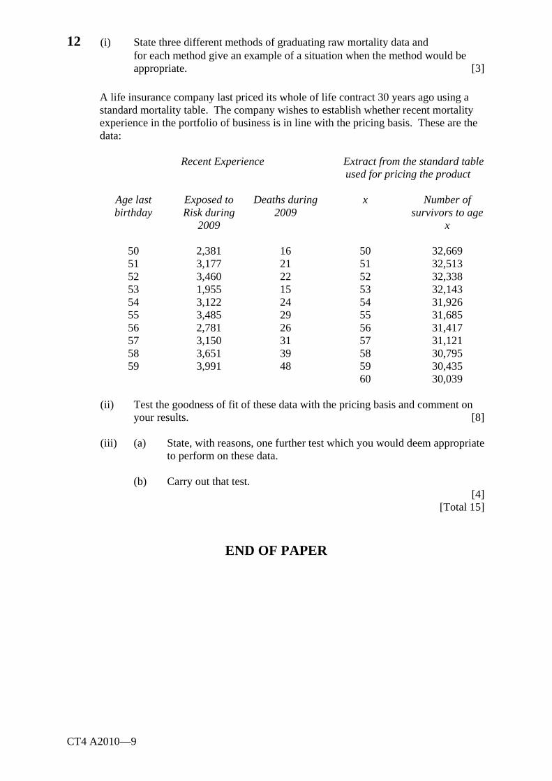
CT4 A2010—9
12 (i) State three different methods of graduating raw mortality data and for each method give an example of a situation when the method would be
appropriate. [3] A life insurance company last priced its whole of life contract 30 years ago using a
standard mortality table. The company wishes to establish whether recent mortality experience in the portfolio of business is in line with the pricing basis. These are the data:
Recent Experience Extract from the standard table
used for pricing the product
Age last birthday
50 51 52 53 54 55 56 57 58 59
Exposed to Risk during
2009
2,381 3,177 3,460 1,955 3,122 3,485 2,781 3,150 3,651 3,991
Deaths during 2009
16 21 22 15 24 29 26 31 39 48
x
50 51 52 53 54 55 56 57 58 59 60
Number of survivors to age
x
32,669 32,513 32,338 32,143 31,926 31,685 31,417 31,121 30,795 30,435 30,039
(ii) Test the goodness of fit of these data with the pricing basis and comment on
your results. [8]
(iii) (a) State, with reasons, one further test which you would deem appropriate to perform on these data.
(b) Carry out that test.
[4] [Total 15]
END OF PAPER
Faculty of Actuaries Institute of Actuaries
EXAMINERS’ REPORT
April 2010 Examinations
Subject CT4 — Models Core Technical
Introduction The attached subject report has been written by the Principal Examiner with the aim of helping candidates. The questions and comments are based around Core Reading as the interpretation of the syllabus to which the examiners are working. They have however given credit for any alternative approach or interpretation which they consider to be reasonable. R D Muckart Chairman of the Board of Examiners July 2010
© Faculty of Actuaries © Institute of Actuaries
Subject CT4 (Models Core Technical) — April 2010 — Examiners’ Report
Page 2
Comments Comments on solutions presented to individual questions for the April 2010 examination paper are given below. In general, those using this report should be aware that in the case of non-numerical answers full credit could often be obtained for rather less than is given in the solutions which follow. The solutions are meant as a guide to the various points which could have been made and considered relevant. Questions without comments in this section were generally well answered, and no specific issues were identified. Q3 A common error was to confuse a Markov Jump Chain with a Markov Jump Process.
A Markov Jump Chain has a discrete time set, whereas the corresponding Markov Jump Process has a continuous time set.
Q4 This was poorly answered. In part (i), many candidates merely gave definitions of the
terms “periodic” and “irreducible”, rather than applying them to the question. In part (ii), many candidates simply drew the three states with arrows denoting all possible transitions between them.
Q5 Answers to this question were disappointing. Many candidates simply wrote down
general lists of the advantages and disadvantages of models, without reference to the problem and the modelling strategy described in the question. Such attempts were given little credit.
Q6 This was a fairly difficult exposed-to-risk question and many candidates found it
challenging. A common error was to include only the first quarter of each employee’s tour of duty in the exposed-to-risk. Many candidates assumed that all accidental deaths happened at the end of each quarter. This seems unrealistic and was penalised, though credit was given for computations of the exposed-to-risk that were correct given this assumption. In part (ii), a large number of candidates made no sensible attempt to analyse their own assumptions made in part (i).
Q8 Parts (iii) and (iv) of this troubled most candidates. Only a minority realised that,
since the Kaplan-Meier estimator is a step function, the point at which S(t) attains the value must lie on one of the “risers” of the steps and therefore be at one of the event durations. In part (iv), many candidates realised that the median estimated in part (iii) included the candidates who had not qualified by the last session of 2009, whereas the median in part (i) did not, but were unable to argue coherently that this meant that the median in part (i) was biased, and under-estimated the true median.
Q9 In part (iv), a disturbingly large number of candidates (the majority) wrote that since
the parameter was positive, the life expectancy must have increased. In fact the opposite is the case. The positive parameter increases the hazard, which leads to a greater risk of death and hence a decline in the birds’ life expectancy in the new enclosure. In part (v) a common error was to assume that 0.1 was the probability of survival, rather than the probability of being killed.

Subject CT4 (Models Core Technical) — April 2010 — Examiners’ Report
Page 3
Q10 In part (iv) a common error was to assume that every member makes exactly one flight. This produces a profit per member of £2.67 compared with the true profit of at least £0.67, and more if some members make more than two flights per year.
Q11 This difficult question was a challenge for almost all candidates. In part (iv) many
candidates simply wrote down the probability rather than deriving it. Credit was given for attempts to part (v) which made use of an integrating factor.
Q12 In part (iii), many candidates chose the Signs Test. Since from the answer to part (ii)
there are five consecutive negative signs followed by five consecutive positive signs it is clear by inspection that the experience will “pass” the Signs Test and so carrying it out is not appropriate. Hence no credit was given for the Signs Test in part (iii)(a). It is much more sensible to conduct a Grouping of Signs Test. As has been the case in previous examinations, the numerical aspects of the tests were generally well performed, but the descriptions of the tests and explanations of what was being done and why were less consistent.
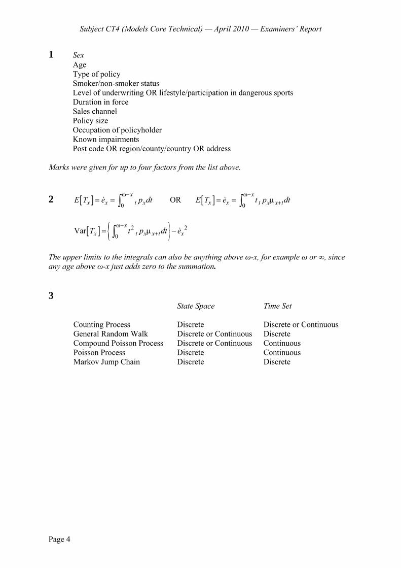
Subject CT4 (Models Core Technical) — April 2010 — Examiners’ Report
Page 4
1 Sex Age Type of policy Smoker/non-smoker status Level of underwriting OR lifestyle/participation in dangerous sports Duration in force Sales channel Policy size Occupation of policyholder Known impairments Post code OR region/county/country OR address Marks were given for up to four factors from the list above.
2 [ ]0
xx x t xE T e p dt
ω−= = ∫ OR [ ]
0
xx x t x x tE T e t p dt
ω−+= = μ∫
[ ] { }2 20
Varx
x t x x t xT t p dt eω−
+= μ −∫
The upper limits to the integrals can also be anything above ω-x, for example ω or ∞, since any age above ω-x just adds zero to the summation. 3
State Space
Time Set
Counting Process Discrete Discrete or Continuous General Random Walk Discrete or Continuous Discrete Compound Poisson Process Discrete or Continuous Continuous Poisson Process Discrete Continuous Markov Jump Chain Discrete Discrete
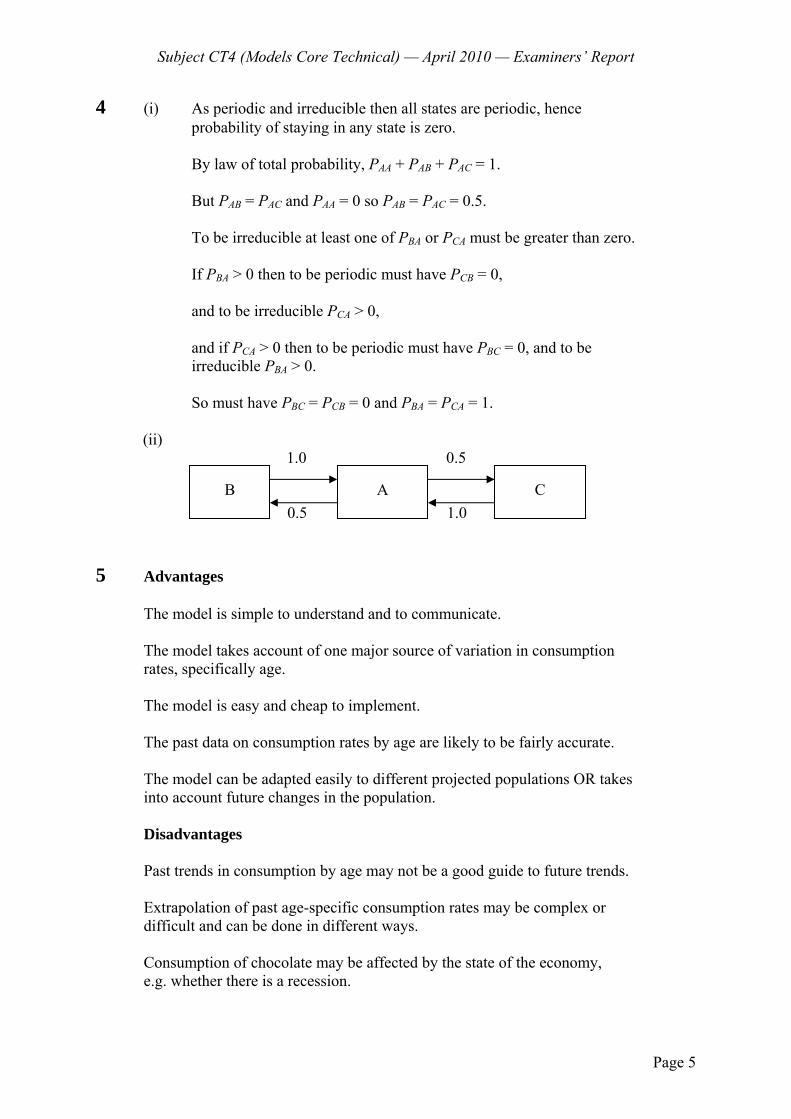
Subject CT4 (Models Core Technical) — April 2010 — Examiners’ Report
Page 5
4 (i) As periodic and irreducible then all states are periodic, hence probability of staying in any state is zero.
By law of total probability, PAA + PAB + PAC = 1. But PAB = PAC and PAA = 0 so PAB = PAC = 0.5. To be irreducible at least one of PBA or PCA must be greater than zero. If PBA > 0 then to be periodic must have PCB = 0, and to be irreducible PCA > 0,
and if PCA > 0 then to be periodic must have PBC = 0, and to be
irreducible PBA > 0.
So must have PBC = PCB = 0 and PBA = PCA = 1.
(ii) 1.0 0.5
0.5 1.0 5 Advantages The model is simple to understand and to communicate. The model takes account of one major source of variation in consumption rates, specifically age. The model is easy and cheap to implement. The past data on consumption rates by age are likely to be fairly accurate. The model can be adapted easily to different projected populations OR takes into account future changes in the population. Disadvantages Past trends in consumption by age may not be a good guide to future trends. Extrapolation of past age-specific consumption rates may be complex or difficult and can be done in different ways. Consumption of chocolate may be affected by the state of the economy, e.g. whether there is a recession.
B A C

Subject CT4 (Models Core Technical) — April 2010 — Examiners’ Report
Page 6
Factors other than age may be important in determining consumption, e.g. expenditure on advertising. Consumption may be sensitive to pricing, which may change in the future. A rapid increase in consumption rates is unlikely to be sustained for a long period as there is likely to be an upper limit to the amount of Scrummy Bars a person can eat.
The projections of the future population by age may not be accurate, as
they depend on future fertility, mortality and migration rates. The proposed strategy does not include any testing of the
sensitivity of total demand to changes in the projected population, or variations in future consumption trends from that used in the model.
Unforeseen events such as competitors launching new products, or the nation becoming increasingly health-aware, may affect future consumption.
The consumption of Scrummy Bars may vary with cohort rather than age, and the model does not capture cohort effects.
Not all the points listed above were required for full credit. Other advantages, for example those related to business prospects, were also given credit. 6 (i) A central exposed to risk for each quarter in person-quarters can be
constructed as follows. In the first quarter there are 90 employees in the first three months of their six-
month tour of duty. Of these 10 will die during the quarter, and these contribute 0.5 each to the exposed to risk.
Therefore the total exposed to risk for the first quarter is 80 + (10 × 0.5) = 85 person-quarters. This assumes that accidental deaths occur on average half way through the quarter in which they were reported. OR that accidental deaths are uniformly distributed across quarters. In the second quarter there are 80 new employees in the first three months of
their six-month tour, and 80 (90 minus the 10 who have died) employees in the second three months of their six-month tour. Of these 8 die during the
quarter, and these contribute 0.5 each to the exposed to risk. Therefore the total exposed to risk for the second quarter is 152 + (8 × 0.5) = 156 person-quarters
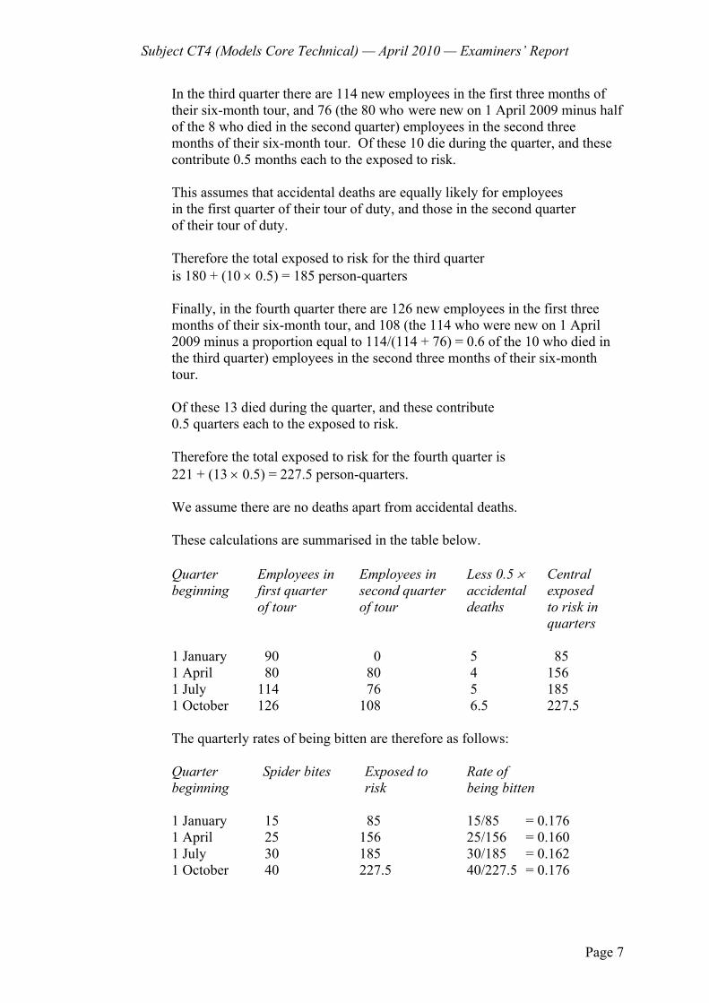
Subject CT4 (Models Core Technical) — April 2010 — Examiners’ Report
Page 7
In the third quarter there are 114 new employees in the first three months of their six-month tour, and 76 (the 80 who were new on 1 April 2009 minus half of the 8 who died in the second quarter) employees in the second three
months of their six-month tour. Of these 10 die during the quarter, and these contribute 0.5 months each to the exposed to risk.
This assumes that accidental deaths are equally likely for employees in the first quarter of their tour of duty, and those in the second quarter of their tour of duty. Therefore the total exposed to risk for the third quarter is 180 + (10 × 0.5) = 185 person-quarters Finally, in the fourth quarter there are 126 new employees in the first three
months of their six-month tour, and 108 (the 114 who were new on 1 April 2009 minus a proportion equal to 114/(114 + 76) = 0.6 of the 10 who died in the third quarter) employees in the second three months of their six-month tour.
Of these 13 died during the quarter, and these contribute 0.5 quarters each to the exposed to risk. Therefore the total exposed to risk for the fourth quarter is 221 + (13 × 0.5) = 227.5 person-quarters. We assume there are no deaths apart from accidental deaths. These calculations are summarised in the table below.
Quarter Employees in Employees in Less 0.5 × Central beginning first quarter second quarter accidental exposed of tour of tour deaths to risk in quarters
1 January 90 0 5 85 1 April 80 80 4 156 1 July 114 76 5 185 1 October 126 108 6.5 227.5
The quarterly rates of being bitten are therefore as follows:
Quarter Spider bites Exposed to Rate of beginning risk being bitten
1 January 15 85 15/85 = 0.176 1 April 25 156 25/156 = 0.160 1 July 30 185 30/185 = 0.162 1 October 40 227.5 40/227.5 = 0.176
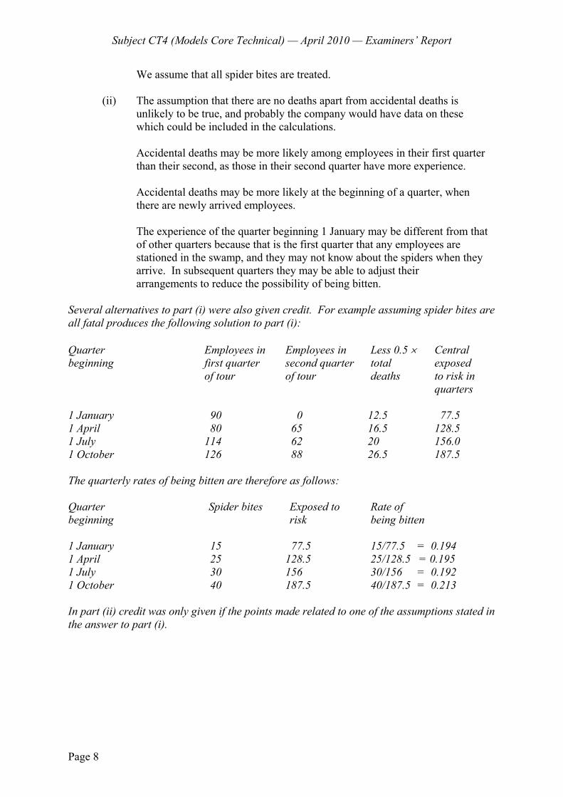
Subject CT4 (Models Core Technical) — April 2010 — Examiners’ Report
Page 8
We assume that all spider bites are treated.
(ii) The assumption that there are no deaths apart from accidental deaths is unlikely to be true, and probably the company would have data on these
which could be included in the calculations. Accidental deaths may be more likely among employees in their first quarter
than their second, as those in their second quarter have more experience. Accidental deaths may be more likely at the beginning of a quarter, when there are newly arrived employees. The experience of the quarter beginning 1 January may be different from that
of other quarters because that is the first quarter that any employees are stationed in the swamp, and they may not know about the spiders when they arrive. In subsequent quarters they may be able to adjust their arrangements to reduce the possibility of being bitten. Several alternatives to part (i) were also given credit. For example assuming spider bites are all fatal produces the following solution to part (i): Quarter Employees in Employees in Less 0.5 × Central beginning first quarter second quarter total exposed of tour of tour deaths to risk in quarters 1 January 90 0 12.5 77.5 1 April 80 65 16.5 128.5 1 July 114 62 20 156.0 1 October 126 88 26.5 187.5 The quarterly rates of being bitten are therefore as follows: Quarter Spider bites Exposed to Rate of beginning risk being bitten 1 January 15 77.5 15/77.5 = 0.194 1 April 25 128.5 25/128.5 = 0.195 1 July 30 156 30/156 = 0.192 1 October 40 187.5 40/187.5 = 0.213 In part (ii) credit was only given if the points made related to one of the assumptions stated in the answer to part (i).
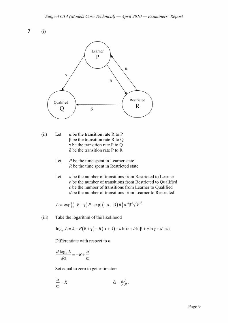
Subject CT4 (Models Core Technical) — April 2010 — Examiners’ Report
Page 9
7 (i)
(ii) Let α be the transition rate R to P β be the transition rate R to Q γ be the transition rate P to Q δ be the transition rate P to R Let P be the time spent in Learner state R be the time spent in Restricted state Let a be the number of transitions from Restricted to Learner b be the number of transitions from Restricted to Qualified c be the number of transitions from Learner to Qualified d be the number of transitions from Learner to Restricted ( ){ } ( ){ }exp exp a b c dL P R∝ −δ − γ −α − β α β γ δ (iii) Take the logarithm of the likelihood ( ) ( )log ln ln ln lne L k P R a b c d= − δ + γ − α + β + α + β + γ + δ Differentiate with respect to α
loged L aRd
= − +α α
Set equal to zero to get estimator:
a R=α
ˆ aRα = .
β
Qualified
Q Restricted
R
Learner
P
γ δ
α
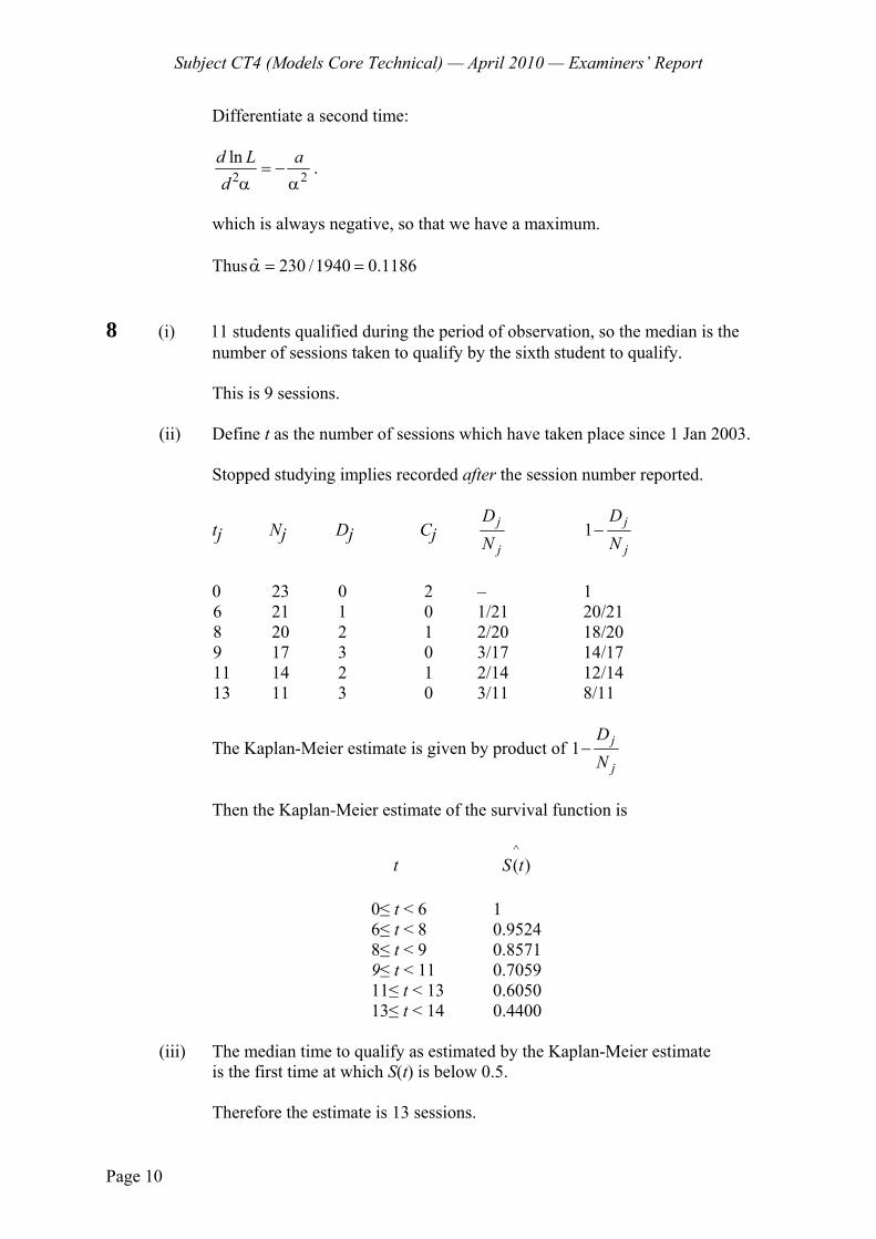
Subject CT4 (Models Core Technical) — April 2010 — Examiners’ Report
Page 10
Differentiate a second time:
2 2lnd L a
d= −
α α.
which is always negative, so that we have a maximum. Thus ˆ 230 /1940 0.1186α = = 8 (i) 11 students qualified during the period of observation, so the median is the
number of sessions taken to qualify by the sixth student to qualify.
This is 9 sessions.
(ii) Define t as the number of sessions which have taken place since 1 Jan 2003.
Stopped studying implies recorded after the session number reported.
tj Nj Dj Cj j
j
DN
1 j
j
DN
−
0 23 0 2 – 1
6 21 1 0 1/21 20/21 8 20 2 1 2/20 18/20 9 17 3 0 3/17 14/17 11 14 2 1 2/14 12/14 13 11 3 0 3/11 8/11
The Kaplan-Meier estimate is given by product of 1 j
j
DN
−
Then the Kaplan-Meier estimate of the survival function is
t ^( )S t
0≤ t < 6 1 6≤ t < 8 0.9524 8≤ t < 9 0.8571 9≤ t < 11 0.7059 11≤ t < 13 0.6050
13≤ t < 14 0.4400 (iii) The median time to qualify as estimated by the Kaplan-Meier estimate
is the first time at which S(t) is below 0.5. Therefore the estimate is 13 sessions.
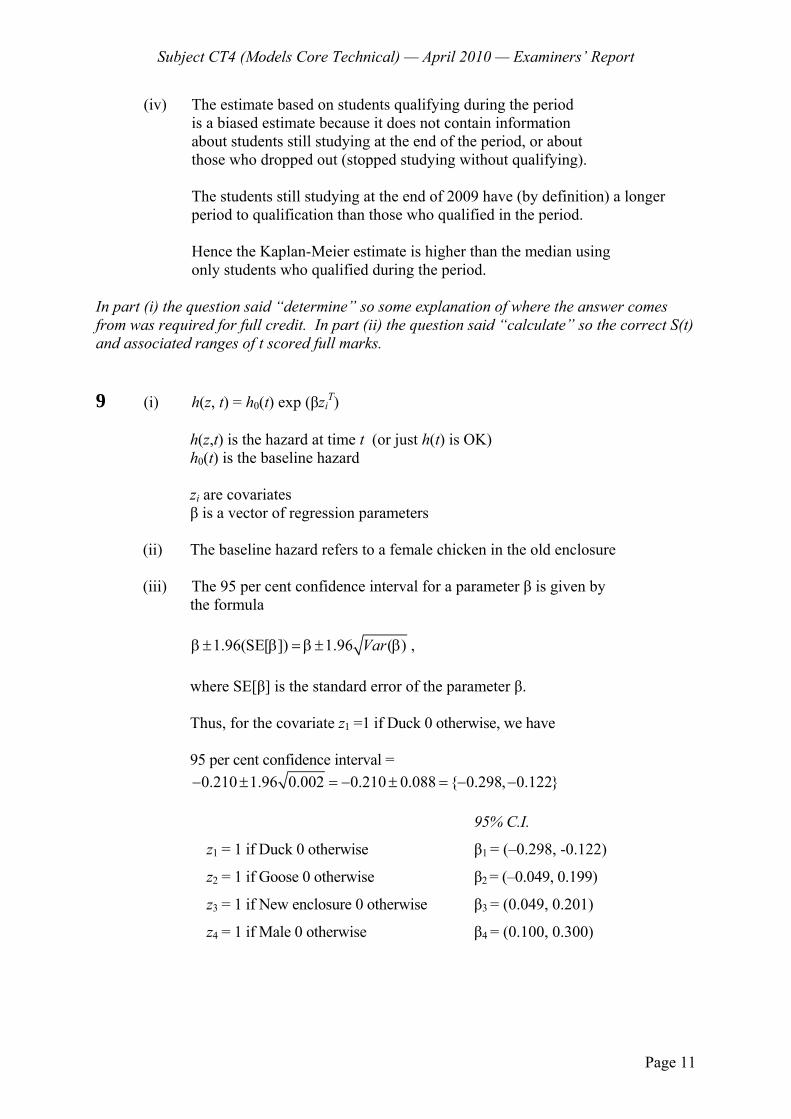
Subject CT4 (Models Core Technical) — April 2010 — Examiners’ Report
Page 11
(iv) The estimate based on students qualifying during the period is a biased estimate because it does not contain information about students still studying at the end of the period, or about those who dropped out (stopped studying without qualifying).
The students still studying at the end of 2009 have (by definition) a longer
period to qualification than those who qualified in the period. Hence the Kaplan-Meier estimate is higher than the median using only students who qualified during the period. In part (i) the question said “determine” so some explanation of where the answer comes from was required for full credit. In part (ii) the question said “calculate” so the correct S(t) and associated ranges of t scored full marks. 9 (i) h(z, t) = h0(t) exp (βzi
T) h(z,t) is the hazard at time t (or just h(t) is OK) h0(t) is the baseline hazard zi are covariates β is a vector of regression parameters (ii) The baseline hazard refers to a female chicken in the old enclosure (iii) The 95 per cent confidence interval for a parameter β is given by the formula 1.96(SE[ ]) 1.96 ( )Varβ ± β = β ± β , where SE[β] is the standard error of the parameter β. Thus, for the covariate z1 =1 if Duck 0 otherwise, we have 95 per cent confidence interval = 0.210 1.96 0.002 0.210 0.088 { 0.298, 0.122}− ± = − ± = − −
z1 = 1 if Duck 0 otherwise
z2 = 1 if Goose 0 otherwise
z3 = 1 if New enclosure 0 otherwise
z4 = 1 if Male 0 otherwise
95% C.I.
β1 = (–0.298, -0.122)
β2 = (–0.049, 0.199)
β3 = (0.049, 0.201)
β4 = (0.100, 0.300)
Subject CT4 (Models Core Technical) — April 2010 — Examiners’ Report
Page 12
(iv) The parameter for the new enclosure is 0.125 so the ratio of the hazard for two otherwise identical birds is exp(0.125) = 1.133. So the hazard appears to have got worse. The 95% confidence interval is entirely positive OR does not include zero so at the 95% level the deterioration is statistically significant. (v) ALTERNATIVE 1 Hazard for a Male, Goose in the Old enclosure is h0(t) exp (0.2 + 0.075 + 0) = h0(t) exp (0.275) Therefore the probability of still being alive in 6 months is
( ) ( )6
Goose 00exp exp 0.275⎡ ⎤= −⎢ ⎥⎣ ⎦∫S h t dt
= ( )6
00exp 1.31653⎡ ⎤−⎢ ⎥⎣ ⎦∫ h t dt
This is equal to 0.9 so
( )6ln 0.9
01.31653 0h t dt= −∫
( )6
000.080028951h t dt =∫
Hazard of a Female, Duck in the New enclosure is 0 0( ) exp(0 0.210 0.125) ( )exp( 0.085)− + = −h t h t So, the probability she is alive after 6 months is
DuckS ( ) ( )6
00exp exp 0.085⎡ ⎤= − −⎢ ⎥⎣ ⎦∫ h t dt
{ }exp 0.080028951(0.918512284)= − { }exp 0.073507574= − = 0.929129 So the probability she’s dead is 0.07087
Subject CT4 (Models Core Technical) — April 2010 — Examiners’ Report
Page 13
ALTERNATIVE 2 Hazard for a Male, Goose in the Old enclosure is h0(t) exp (0.2 + 0.075 + 0) = h0(t) exp (0.275) Therefore the probability of still being alive in 6 months is
( ) ( )6
Goose 00exp exp 0.275⎡ ⎤= −⎢ ⎥⎣ ⎦∫S h t dt
Similarly, the probability of still being alive in 6 months for A Female Duck in the New enclosure is
DuckS ( ) ( )6
00exp exp 0.085⎡ ⎤= − −⎢ ⎥⎣ ⎦∫ h t dt .
Therefore we can write
( ) ( )
( ) ( )
6
00Goose6
Duck 00
exp exp 0.275
exp exp 0.085
h t dtSS h t dt
⎡ ⎤−⎢ ⎥⎣ ⎦=⎡ ⎤− −⎢ ⎥⎣ ⎦
∫
∫,
whence
( ) ( )
( ) ( )
6
00Goose6
Duck 00
exp 0.275log exp(0.275) .log exp( 0.085)exp 0.085
e
e
h t dtSS h t dt
−= =
−− −
∫∫
Hence
GooseDuck
log [exp( 0.085)]log .exp(0.275)
ee
SS −=
Since SGoose = 0.9, therefore
Ducklog 0.9[exp( 0.085)]log 0.07351
exp(0.275)e
e S −= = −
So SDuck = 0.929129 So the probability she’s dead is 0.07087
Subject CT4 (Models Core Technical) — April 2010 — Examiners’ Report
Page 14
10 (i) (a) The state space is discrete (with four states: O – ordinary passenger, B – bronze member, S – silver member and G – gold member)
The probability that a passenger has a particular membership
status next year depends only on their membership status in the current year (i.e. the status in previous years is not relevant).
Therefore the process is Markov.
(b) The state space is finite and therefore there is at least one stationary probability distribution. Since any state can be reached from any other state, the
Markov chain is irreducible.
Therefore the stationary probability distribution is unique.
(ii) The transition matrix P is:
0 1 2
0 1 2
0 1 2
0 1 2
0 00
00 0
p p pOp p pB
p p pSp p pG
+
+
+
+
+⎛ ⎞⎜ ⎟⎜ ⎟⎜ ⎟⎜ ⎟
+⎝ ⎠
where the probability that a passenger books i flights in a year is ip .
(iii) Let the probability that a passenger is in state j according to the stationary distribution be jπ ( , , ,j O B S G= ).
The jπ are given by the general formula
Pπ = π .
With 0 0.4p = , 1 0.4p = and 2 0.2p + = , we therefore have the equations
0.8 0.4O O Bπ = π + π (1)
0.2 0.4 0.4B O B Sπ = π + π + π (2) 0.2 0.4 0.4S B S Gπ = π + π + π (3) 0.2 0.6G S Gπ = π + π (4)
We also know that
1O B S Gπ + π + π + π = .
Subject CT4 (Models Core Technical) — April 2010 — Examiners’ Report
Page 15
Using equation (1) we have
0.2 0.4O Bπ = π
so that
2O Bπ = π .
Substituting in equation (2) this yields
0.2(2 ) 0.4 0.4B B B Sπ = π + π + π ,
so that
0.2 0.4B Sπ = π
and hence
0.5S Bπ = π .
Finally, substituting in equation (3) yields
0.5 0.2 0.4(0.5 ) 0.4B B B Gπ = π + π + π ,
so that
0.1 0.4B Gπ = π
and hence
0.25G Bπ = π .
We therefore have
2 0.5 0.25 1B B B Bπ + π + π + π = ,
whence
1 4 0.26673.75 15Bπ = = = ,
and the stationary distribution is
8 0.533315Oπ = =

Subject CT4 (Models Core Technical) — April 2010 — Examiners’ Report
Page 16
4 0.266715Bπ = =
2 0.1333
15Sπ = =
1 0.0667
15Gπ = =
(iv) EITHER
The expected cost of the scheme per member per year is (0 × 0.5333) + (£10 × 0.2667) + (£20 × 0.1333) + (£30 × 0.0667) = £7.33 For the scheme to be worth running, therefore, the average profit
per member per year must exceed £7.33. The profit per member is 0 for the 40% who book no flights,
£10 for the 40% who book one flight, and £10m for the 20% who book two or more flights, where m is the average number of flights booked by those in the latter category.
For there to be a profit, we must have
(0.4 × 0) + (0.4 × £10) + (0.2 × £10m) > 7.33
or
4 + 2m > 7.33
2m > 3.33 m > 1.67 This must be the case since m cannot be less than 2. Therefore the airline makes a profit on the members of the scheme. OR Assuming that the distribution of the number of flights taken
is the same for all membership statuses, then for an Ordinary member the expected profit is (0.4 × 0) + (0.4 × 10) + (0.2 × 20) = £8
Similarly for the other classes of member the expected profit is
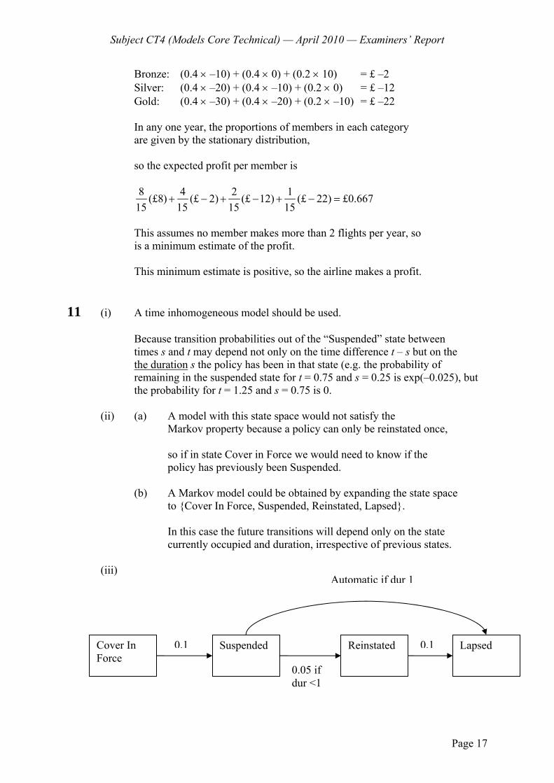
Subject CT4 (Models Core Technical) — April 2010 — Examiners’ Report
Page 17
Bronze: (0.4 × –10) + (0.4 × 0) + (0.2 × 10) = £ –2 Silver: (0.4 × –20) + (0.4 × –10) + (0.2 × 0) = £ –12 Gold: (0.4 × –30) + (0.4 × –20) + (0.2 × –10) = £ –22 In any one year, the proportions of members in each category are given by the stationary distribution, so the expected profit per member is
8 4 2 1(£8) (£ 2) (£ 12) (£ 22) £0.66715 15 15 15
+ − + − + − =
This assumes no member makes more than 2 flights per year, so
is a minimum estimate of the profit.
This minimum estimate is positive, so the airline makes a profit. 11 (i) A time inhomogeneous model should be used. Because transition probabilities out of the “Suspended” state between
times s and t may depend not only on the time difference t – s but on the the duration s the policy has been in that state (e.g. the probability of remaining in the suspended state for t = 0.75 and s = 0.25 is exp(–0.025), but the probability for t = 1.25 and s = 0.75 is 0.
(ii) (a) A model with this state space would not satisfy the
Markov property because a policy can only be reinstated once,
so if in state Cover in Force we would need to know if the policy has previously been Suspended.
(b) A Markov model could be obtained by expanding the state space
to {Cover In Force, Suspended, Reinstated, Lapsed}. In this case the future transitions will depend only on the state
currently occupied and duration, irrespective of previous states.
(iii)
Cover In Force
Suspended Reinstated Lapsed 0.1 0.1
0.05 if dur <1
Automatic if dur 1
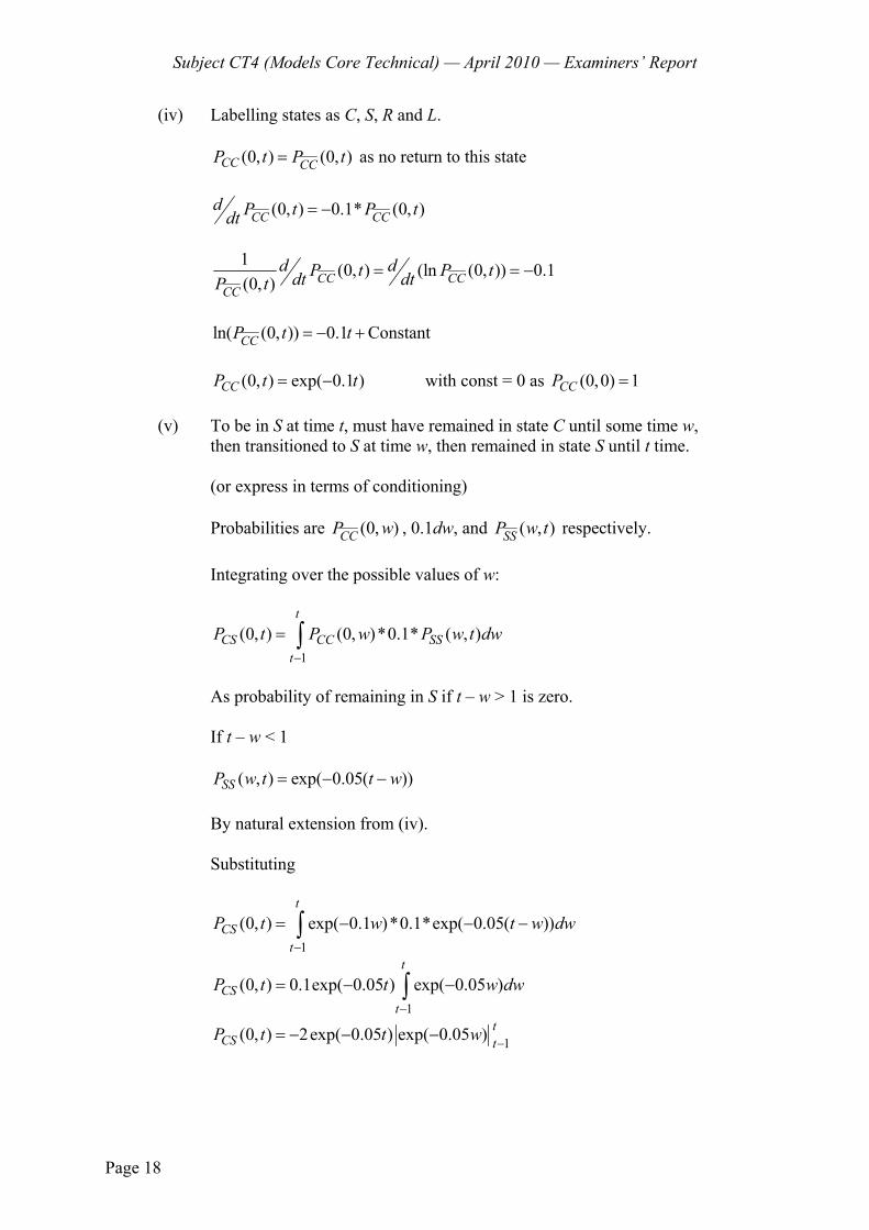
Subject CT4 (Models Core Technical) — April 2010 — Examiners’ Report
Page 18
(iv) Labelling states as C, S, R and L.
(0, ) (0, )CC CCP t P t= as no return to this state
(0, ) 0.1* (0, )CC CCd P t P tdt = −
1 (0, ) (ln (0, )) 0.1(0, ) CC CC
CC
d dP t P tdt dtP t= = −
ln( (0, )) 0.1 ConstantCCP t t= − + (0, ) exp( 0.1 )CCP t t= − with const = 0 as (0,0) 1CCP =
(v) To be in S at time t, must have remained in state C until some time w,
then transitioned to S at time w, then remained in state S until t time. (or express in terms of conditioning)
Probabilities are (0, )CCP w , 0.1dw, and ( , )SSP w t respectively.
Integrating over the possible values of w:
1
(0, ) (0, )*0.1* ( , )t
CS CC SSt
P t P w P w t dw−
= ∫
As probability of remaining in S if t – w > 1 is zero.
If t – w < 1
( , ) exp( 0.05( ))SSP w t t w= − −
By natural extension from (iv).
Substituting
1
(0, ) exp( 0.1 )*0.1*exp( 0.05( ))t
CSt
P t w t w dw−
= − − −∫
1
(0, ) 0.1exp( 0.05 ) exp( 0.05 )t
CSt
P t t w dw−
= − −∫
1(0, ) 2exp( 0.05 ) exp( 0.05 ) tCS tP t t w −= − − −
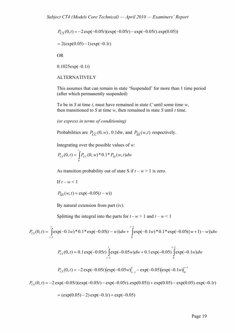
Subject CT4 (Models Core Technical) — April 2010 — Examiners’ Report
Page 19
(0, ) 2exp( 0.05 )(exp( 0.05 ) exp( 0.05 ).exp(0.05))= − − − − −CSP t t t t
2(exp(0.05) 1)exp( 0.1 )= − − t OR
0.1025exp(–0.1t) ALTERNATIVELY This assumes that can remain in state ‘Suspended’ for more than 1 time period (after which permanently suspended)
To be in S at time t, must have remained in state C until some time w,
then transitioned to S at time w, then remained in state S until t time.
(or express in terms of conditioning) Probabilities are (0, )CCP w , 0.1dw, and ( , )SSP w t respectively.
Integrating over the possible values of w:
∫=t
SSCCCS dwtwPwPtP0
),(*1.0*),0(),0(
As transition probability out of state S if t – w > 1 is zero.
If t – w < 1
( , ) exp( 0.05( ))SSP w t t w= − −
By natural extension from part (iv).
Splitting the integral into the parts for t - w > 1 and t – w < 1
∫∫−
−
−+−−+−−−=1
01
)))1((05.0exp(*1.0*)1.0exp())(05.0exp(*1.0*)1.0exp(),0(tt
tCS dwwwwdwwtwtP
∫∫−
−
−−+−−=1
01
)1.0exp()05.0exp(1.0)05.0exp()05.0exp(1.0),0(tt
tCS dwwdwwttP
1
01)1.0exp()05.0exp()05.0exp()05.0exp(2),0( −
−−−−−−−= tt
tCS wwttP
)1.0exp().05.0exp()05.0exp())05.0exp().05.0exp()05.0)(exp(05.0exp(2),0( tttttPCS −−+−−−−−= )05.0exp()1.0exp()2)05.0(exp( −+−−= t
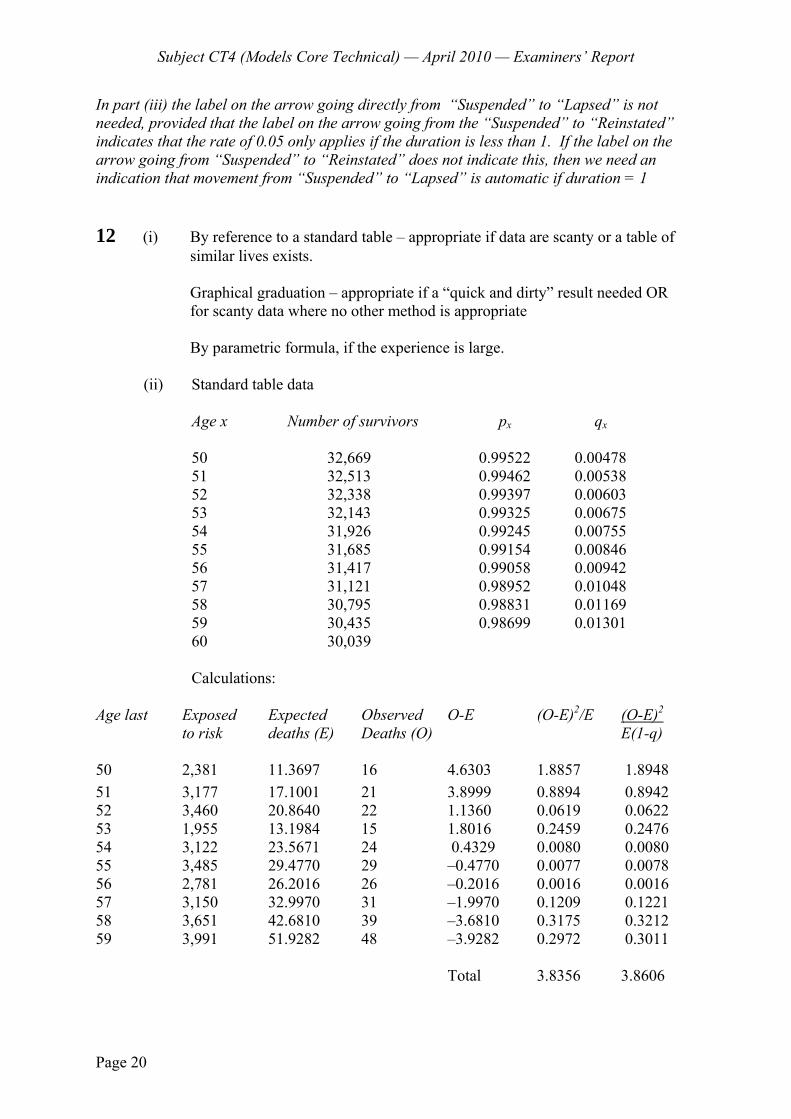
Subject CT4 (Models Core Technical) — April 2010 — Examiners’ Report
Page 20
In part (iii) the label on the arrow going directly from “Suspended” to “Lapsed” is not needed, provided that the label on the arrow going from the “Suspended” to “Reinstated” indicates that the rate of 0.05 only applies if the duration is less than 1. If the label on the arrow going from “Suspended” to “Reinstated” does not indicate this, then we need an indication that movement from “Suspended” to “Lapsed” is automatic if duration = 1 12 (i) By reference to a standard table – appropriate if data are scanty or a table of similar lives exists. Graphical graduation – appropriate if a “quick and dirty” result needed OR for scanty data where no other method is appropriate By parametric formula, if the experience is large.
(ii) Standard table data Age x Number of survivors px qx
50 32,669 0.99522 0.00478 51 32,513 0.99462 0.00538 52 32,338 0.99397 0.00603 53 32,143 0.99325 0.00675 54 31,926 0.99245 0.00755 55 31,685 0.99154 0.00846 56 31,417 0.99058 0.00942 57 31,121 0.98952 0.01048 58 30,795 0.98831 0.01169 59 30,435 0.98699 0.01301 60 30,039
Calculations: Age last Exposed
to risk
Expected deaths (E)
Observed Deaths (O)
O-E (O-E)2/E (O-E)2 E(1-q)
50 2,381 11.3697 16 4.6303 1.8857 1.8948 51 3,177 17.1001 21 3.8999 0.8894 0.8942 52 3,460 20.8640 22 1.1360 0.0619 0.0622 53 1,955 13.1984 15 1.8016 0.2459 0.2476 54 3,122 23.5671 24 0.4329 0.0080 0.0080 55 3,485 29.4770 29 –0.4770 0.0077 0.0078 56 2,781 26.2016 26 –0.2016 0.0016 0.0016 57 3,150 32.9970 31 –1.9970 0.1209 0.1221 58 3,651 42.6810 39 –3.6810 0.3175 0.3212 59 3,991 51.9282 48 –3.9282 0.2972 0.3011
Total 3.8356 3.8606
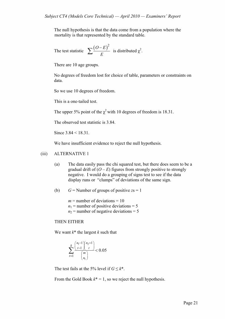
Subject CT4 (Models Core Technical) — April 2010 — Examiners’ Report
Page 21
The null hypothesis is that the data come from a population where the mortality is that represented by the standard table.
The test statistic ( )2O EE−
∑ is distributed χ2.
There are 10 age groups. No degrees of freedom lost for choice of table, parameters or constraints on
data. So we use 10 degrees of freedom. This is a one-tailed test. The upper 5% point of the χ2 with 10 degrees of freedom is 18.31. The observed test statistic is 3.84. Since 3.84 < 18.31. We have insufficient evidence to reject the null hypothesis. (iii) ALTERNATIVE 1 (a) The data easily pass the chi squared test, but there does seem to be a
gradual drift of (O – E) figures from strongly positive to strongly negative. I would do a grouping of signs test to see if the data
display runs or “clumps” of deviations of the same sign. (b) G = Number of groups of positive zs = 1 m = number of deviations = 10 n1 = number of positive deviations = 5 n2 = number of negative deviations = 5 THEN EITHER We want k* the largest k such that
1 2
1
1 11
10.05
− +⎛ ⎞⎛ ⎞⎜ ⎟⎜ ⎟−⎝ ⎠⎝ ⎠
⎛ ⎞= ⎜ ⎟
⎝ ⎠
<∑n n
kt t
mt n
The test fails at the 5% level if G ≤ k*. From the Gold Book k* = 1, so we reject the null hypothesis.
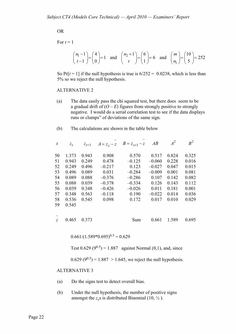
Subject CT4 (Models Core Technical) — April 2010 — Examiners’ Report
Page 22
OR For t = 1
1 2
1
1 4 1 6 101 and 6 and 252
1 0 1 5mn nnt t
− + ⎛ ⎞⎛ ⎞ ⎛ ⎞ ⎛ ⎞ ⎛ ⎞ ⎛ ⎞= = = = = =⎜ ⎟⎜ ⎟ ⎜ ⎟ ⎜ ⎟ ⎜ ⎟ ⎜ ⎟−⎝ ⎠ ⎝ ⎠ ⎝ ⎠ ⎝ ⎠ ⎝ ⎠⎝ ⎠
So Pr[t = 1] if the null hypothesis is true is 6/252 = 0.0238, which is less than
5% so we reject the null hypothesis. ALTERNATIVE 2 (a) The data easily pass the chi squared test, but there does seem to be a gradual drift of (O – E) figures from strongly positive to strongly
negative. I would do a serial correlation test to see if the data displays runs or clumps” of deviations of the same sign.
(b) The calculations are shown in the table below
x zx zx+1 xA z z−
= − 1xB z z−
+= − AB 2A 2B
50 1.373 0.943 0.908 0.570 0.517 0.824 0.325 51 0.943 0.249 0.478 –0.125 –0.060 0.228 0.016 52 0.249 0.496 –0.217 0.123 –0.027 0.047 0.015 53 0.496 0.089 0.031 –0.284 –0.009 0.001 0.081 54 0.089 0.088 –0.376 –0.286 0.107 0.142 0.082 55 0.088 0.039 –0.378 –0.334 0.126 0.143 0.112 56 0.039 0.348 –0.426 –0.026 0.011 0.181 0.001 57 0.348 0.563 –0.118 0.190 –0.022 0.014 0.036 58 0.536 0.545 0.098 0.172 0.017 0.010 0.029 59 0.545
z−
0.465 0.373 Sum 0.661 1.589 0.695 0.661/(1.589*0.695)0.5 = 0.629 Test 0.629 (90.5) = 1.887 against Normal (0,1), and, since 0.629 (90.5) = 1.887 > 1.645, we reject the null hypothesis. ALTERNATIVE 3 (a) Do the signs test to detect overall bias. (b) Under the null hypothesis, the number of positive signs amongst the zxs is distributed Binomial (10, ½ ).
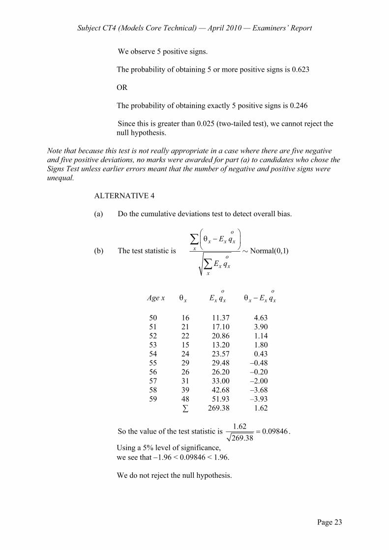
Subject CT4 (Models Core Technical) — April 2010 — Examiners’ Report
Page 23
We observe 5 positive signs. The probability of obtaining 5 or more positive signs is 0.623
OR
The probability of obtaining exactly 5 positive signs is 0.246
Since this is greater than 0.025 (two-tailed test), we cannot reject the
null hypothesis. Note that because this test is not really appropriate in a case where there are five negative and five positive deviations, no marks were awarded for part (a) to candidates who chose the Signs Test unless earlier errors meant that the number of negative and positive signs were unequal. ALTERNATIVE 4
(a) Do the cumulative deviations test to detect overall bias.
(b) The test statistic is Normal(0,1)
ox x x
xo
x xx
E q
E q
⎛ ⎞θ −⎜ ⎟
⎝ ⎠∑
∑∼
Age x xθ o
x xE q o
x x xE qθ − 50 16 11.37 4.63 51 21 17.10 3.90 52 22 20.86 1.14 53 15 13.20 1.80 54 24 23.57 0.43 55 29 29.48 –0.48 56 26 26.20 –0.20 57 31 33.00 –2.00 58 39 42.68 –3.68 59 48 51.93 –3.93 ∑ 269.38 1.62
So the value of the test statistic is 1.62 0.09846269.38
= .
Using a 5% level of significance, we see that −1.96 < 0.09846 < 1.96.
We do not reject the null hypothesis.
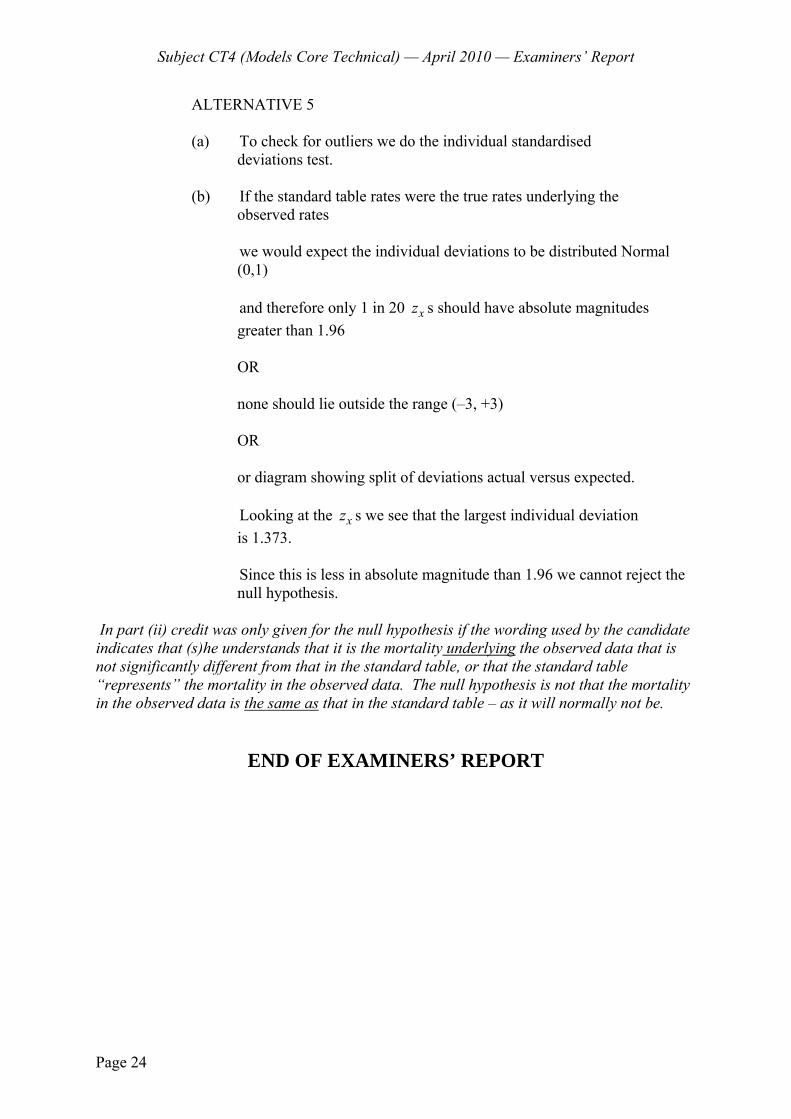
Subject CT4 (Models Core Technical) — April 2010 — Examiners’ Report
Page 24
ALTERNATIVE 5
(a) To check for outliers we do the individual standardised deviations test.
(b) If the standard table rates were the true rates underlying the observed rates
we would expect the individual deviations to be distributed Normal (0,1)
and therefore only 1 in 20 xz s should have absolute magnitudes
greater than 1.96 OR
none should lie outside the range (–3, +3) OR
or diagram showing split of deviations actual versus expected.
Looking at the xz s we see that the largest individual deviation
is 1.373. Since this is less in absolute magnitude than 1.96 we cannot reject the
null hypothesis. In part (ii) credit was only given for the null hypothesis if the wording used by the candidate indicates that (s)he understands that it is the mortality underlying the observed data that is not significantly different from that in the standard table, or that the standard table “represents” the mortality in the observed data. The null hypothesis is not that the mortality in the observed data is the same as that in the standard table – as it will normally not be.
END OF EXAMINERS’ REPORT

Faculty of Actuaries Institute of Actuaries
EXAMINATION
1 October 2010 (am)
Subject CT4 — Models Core Technical
Time allowed: Three hours
INSTRUCTIONS TO THE CANDIDATE
1. Enter all the candidate and examination details as requested on the front of your answer booklet.
2. You must not start writing your answers in the booklet until instructed to do so by the
supervisor. 3. Mark allocations are shown in brackets. 4. Attempt all 12 questions, beginning your answer to each question on a separate sheet. 5. Candidates should show calculations where this is appropriate.
Graph paper is NOT required for this paper.
AT THE END OF THE EXAMINATION
Hand in BOTH your answer booklet, with any additional sheets firmly attached, and this question paper.
In addition to this paper you should have available the 2002 edition of the Formulae and Tables and your own electronic calculator from the approved list.
© Faculty of Actuaries CT4 S2010 © Institute of Actuaries
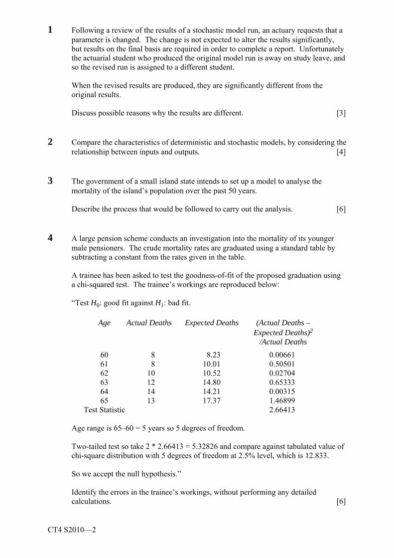
CT4 S2010—2
1 Following a review of the results of a stochastic model run, an actuary requests that a parameter is changed. The change is not expected to alter the results significantly, but results on the final basis are required in order to complete a report. Unfortunately the actuarial student who produced the original model run is away on study leave, and so the revised run is assigned to a different student.
When the revised results are produced, they are significantly different from the
original results. Discuss possible reasons why the results are different. [3]
2 Compare the characteristics of deterministic and stochastic models, by considering the relationship between inputs and outputs. [4]
3 The government of a small island state intends to set up a model to analyse the
mortality of the island’s population over the past 50 years. Describe the process that would be followed to carry out the analysis. [6] 4 A large pension scheme conducts an investigation into the mortality of its younger
male pensioners. The crude mortality rates are graduated using a standard table by subtracting a constant from the rates given in the table.
A trainee has been asked to test the goodness-of-fit of the proposed graduation using a chi-squared test. The trainee’s workings are reproduced below:
“Test H0: good fit against H1: bad fit.
Age Actual Deaths Expected Deaths (Actual Deaths – Expected Deaths)2
/Actual Deaths 60 8 8.23 0.00661 61 8 10.01 0.50501 62 10 10.52 0.02704 63 12 14.80 0.65333 64 14 14.21 0.00315 65 13 17.37 1.46899 Test Statistic 2.66413
Age range is 65–60 = 5 years so 5 degrees of freedom. Two-tailed test so take 2 * 2.66413 = 5.32826 and compare against tabulated value of chi-square distribution with 5 degrees of freedom at 2.5% level, which is 12.833.
So we accept the null hypothesis.”
Identify the errors in the trainee’s workings, without performing any detailed
calculations. [6]
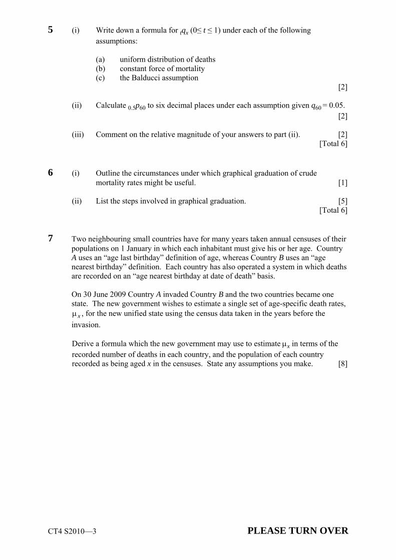
CT4 S2010—3 PLEASE TURN OVER
5 (i) Write down a formula for tqx (0≤ t ≤ 1) under each of the following assumptions:
(a) uniform distribution of deaths (b) constant force of mortality (c) the Balducci assumption
[2] (ii) Calculate 0.5p60 to six decimal places under each assumption given q60 = 0.05.
[2] (iii) Comment on the relative magnitude of your answers to part (ii). [2] [Total 6] 6 (i) Outline the circumstances under which graphical graduation of crude mortality rates might be useful. [1] (ii) List the steps involved in graphical graduation. [5] [Total 6]
7 Two neighbouring small countries have for many years taken annual censuses of their populations on 1 January in which each inhabitant must give his or her age. Country A uses an “age last birthday” definition of age, whereas Country B uses an “age nearest birthday” definition. Each country has also operated a system in which deaths are recorded on an “age nearest birthday at date of death” basis. On 30 June 2009 Country A invaded Country B and the two countries became one state. The new government wishes to estimate a single set of age-specific death rates,
xμ , for the new unified state using the census data taken in the years before the invasion.
Derive a formula which the new government may use to estimate μx in terms of the recorded number of deaths in each country, and the population of each country recorded as being aged x in the censuses. State any assumptions you make. [8]
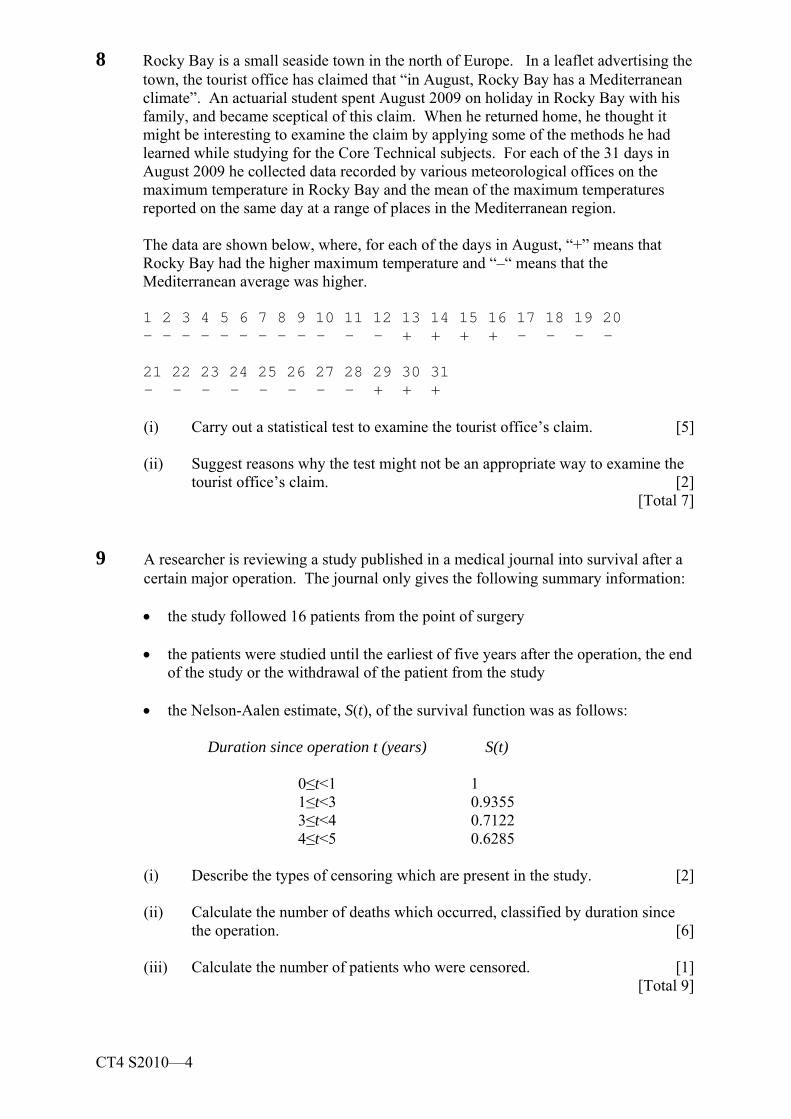
CT4 S2010—4
8 Rocky Bay is a small seaside town in the north of Europe. In a leaflet advertising the town, the tourist office has claimed that “in August, Rocky Bay has a Mediterranean climate”. An actuarial student spent August 2009 on holiday in Rocky Bay with his family, and became sceptical of this claim. When he returned home, he thought it might be interesting to examine the claim by applying some of the methods he had learned while studying for the Core Technical subjects. For each of the 31 days in August 2009 he collected data recorded by various meteorological offices on the maximum temperature in Rocky Bay and the mean of the maximum temperatures reported on the same day at a range of places in the Mediterranean region.
The data are shown below, where, for each of the days in August, “+” means that
Rocky Bay had the higher maximum temperature and “–“ means that the Mediterranean average was higher.
1 2 3 4 5 6 7 8 9 10 11 12 13 14 15 16 17 18 19 20 - - - - - - - - - - - - + + + + - - - -
21 22 23 24 25 26 27 28 29 30 31 - - - - - - - - + + + (i) Carry out a statistical test to examine the tourist office’s claim. [5] (ii) Suggest reasons why the test might not be an appropriate way to examine the
tourist office’s claim. [2] [Total 7]
9 A researcher is reviewing a study published in a medical journal into survival after a certain major operation. The journal only gives the following summary information:
• the study followed 16 patients from the point of surgery
• the patients were studied until the earliest of five years after the operation, the end
of the study or the withdrawal of the patient from the study
• the Nelson-Aalen estimate, S(t), of the survival function was as follows:
Duration since operation t (years) S(t)
0≤t<1 1 1≤t<3 0.9355
3≤t<4 0.7122 4≤t<5 0.6285
(i) Describe the types of censoring which are present in the study. [2] (ii) Calculate the number of deaths which occurred, classified by duration since
the operation. [6] (iii) Calculate the number of patients who were censored. [1] [Total 9]
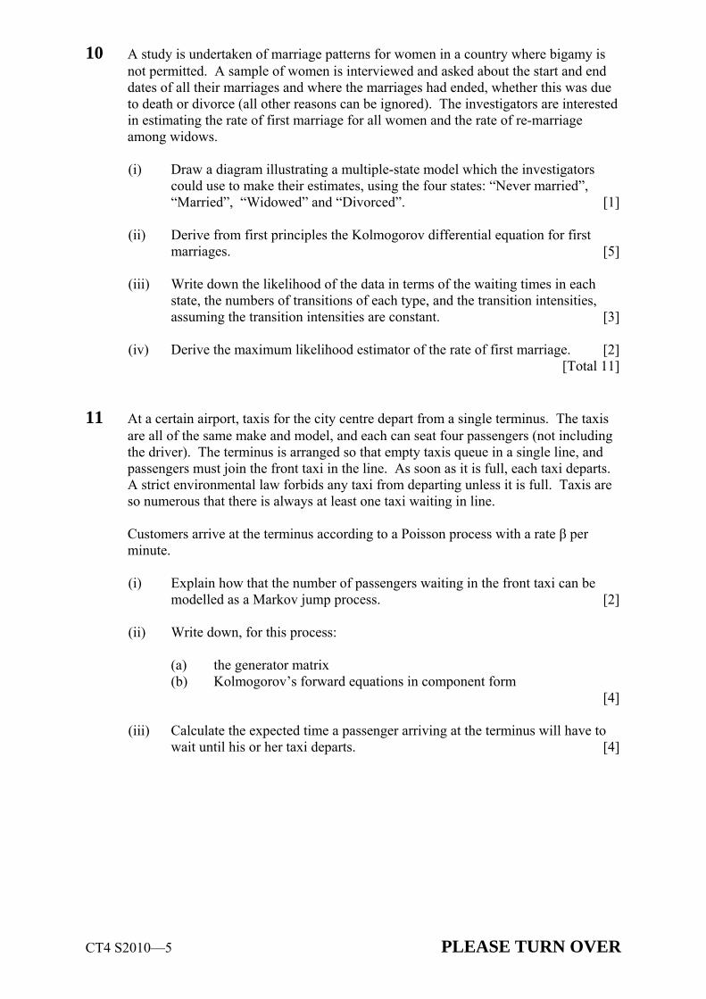
CT4 S2010—5 PLEASE TURN OVER
10 A study is undertaken of marriage patterns for women in a country where bigamy is not permitted. A sample of women is interviewed and asked about the start and end dates of all their marriages and where the marriages had ended, whether this was due to death or divorce (all other reasons can be ignored). The investigators are interested in estimating the rate of first marriage for all women and the rate of re-marriage among widows.
(i) Draw a diagram illustrating a multiple-state model which the investigators could use to make their estimates, using the four states: “Never married”, “Married”, “Widowed” and “Divorced”. [1]
(ii) Derive from first principles the Kolmogorov differential equation for first
marriages. [5]
(iii) Write down the likelihood of the data in terms of the waiting times in each state, the numbers of transitions of each type, and the transition intensities, assuming the transition intensities are constant. [3]
(iv) Derive the maximum likelihood estimator of the rate of first marriage. [2] [Total 11] 11 At a certain airport, taxis for the city centre depart from a single terminus. The taxis
are all of the same make and model, and each can seat four passengers (not including the driver). The terminus is arranged so that empty taxis queue in a single line, and passengers must join the front taxi in the line. As soon as it is full, each taxi departs. A strict environmental law forbids any taxi from departing unless it is full. Taxis are so numerous that there is always at least one taxi waiting in line. Customers arrive at the terminus according to a Poisson process with a rate β per minute.
(i) Explain how that the number of passengers waiting in the front taxi can be modelled as a Markov jump process. [2]
(ii) Write down, for this process:
(a) the generator matrix (b) Kolmogorov’s forward equations in component form
[4]
(iii) Calculate the expected time a passenger arriving at the terminus will have to wait until his or her taxi departs. [4]

CT4 S2010—6
The four-passenger taxis were highly polluting, and the government instituted a “scrappage” scheme whereby taxi drivers were given a subsidy to replace their old four-passenger taxis with new “greener” models. Two such models were on the market, one of which had a capacity of three passengers and the other of which had a capacity of five passengers (again, not including the driver in each case). Half the taxis were replaced with three-passenger models, and half with five-passenger models. Assume that, after the replacement, three-passenger and five-passenger models arrive randomly at the terminus.
(iv) Write down the transition matrix of the Markov jump chain describing the
number of passengers in the front taxi after the vehicle replacement. [2] (v) Calculate the expected waiting time for a passenger arriving at the terminus
after the vehicle scrappage scheme and compare this with your answer to part (iii). [3]
[Total 15] 12 A pet shop has four glass tanks in which snakes for sale are held. The shop can stock
at most four snakes at any one time because:
• if more than one snake were held in the same tank, the snakes would attempt to eat each other and
• having snakes loose in the shop would not be popular with the neighbours
The number of snakes sold by the shop each day is a random variable with the following distribution:
Number of Snakes Potentially Sold Probability in Day (if stock is sufficient) None 0.4 One 0.4 Two 0.2
If the shop has no snakes in stock at the end of a day, the owner contacts his snake supplier to order four more snakes. The snakes are delivered the following morning before the shop opens. The snake supplier makes a charge of C for the delivery.
(i) Write down the transition matrix for the number of snakes in stock when the
shop opens in a morning, given the number in stock when the shop opened the previous day. [2]
(ii) Calculate the stationary distribution for the number of snakes in stock when
the shop opens, using your transition matrix in part (i). [4] (iii) Calculate the expected long term average number of restocking orders placed
by the shop owner per trading day. [2]
CT4 S2010—7
If a customer arrives intending to purchase a snake, and there is none in stock, the sale is lost to a rival pet shop.
(iv) Calculate the expected long term number of sales lost per trading day. [2]
The owner is unhappy about losing these sales as there is a profit on each sale of P. He therefore considers changing his restocking approach to place an order before he has run out of snakes. The charge for the delivery remains at C irrespective of how many snakes are delivered. (v) Evaluate the expected number of restocking orders, and number of lost sales per trading day, if the owner decides to restock if there are fewer than two snakes remaining in stock at the end of the day. [5]
(vi) Explain why restocking when two or more snakes remain in stock cannot
optimise the shop’s profits. [2] The pet shop owner wishes to maximise the profit he makes on snakes. (vii) Derive a condition in terms of C and P under which the owner should change
from only restocking where there are no snakes in stock, to restocking when there are fewer than two snakes in stock. [2]
[Total 19]
END OF PAPER
Page 1
INSTITUTE AND FACULTY OF ACTUARIES
EXAMINERS’ REPORT
September 2010 examinations
Subject CT4 — Models Core Technical
Introduction The attached subject report has been written by the Principal Examiner with the aim of helping candidates. The questions and comments are based around Core Reading as the interpretation of the syllabus to which the examiners are working. They have however given credit for any alternative approach or interpretation which they consider to be reasonable. T J Birse Chairman of the Board of Examiners December 2010
© Institute and Faculty of Actuaries

Subject CT4 (Models Core Technical) — September 2010 — Examiners’ Report
Page 2
Question 1 One or both of the runs (the original or the new) may have been incorrect as, for example, the second trainee may not have been fully aware of the set-up (for example he or she may not have followed the procedure correctly, or may have used different assumptions) The difference between the two runs may not have only been the parameter change, for example the two runs may have used different random seeds, or the second run may have had fewer simulations. The expectation that the model was not sensitive to this parameter could have been incorrect. Other valid points were given credit, for example that some parameters might be linked to live data, which will necessarily have changed; or that there may have been other amendments to the data in the meantime. However, the maximum number of marks attainable on this question was 3. Question 2 A deterministic model is a model which does not contain any random components. The output is determined once the fixed inputs and the relationships between inputs and outputs have been defined. A stochastic model is one that recognises the random nature of the input components. The inputs to a stochastic model are random variables, and hence for any given values of the inputs the outputs are an estimate of the characteristics of the model. Several independent iterations of the model are required for each set of inputs to study their implications. The output of a stochastic model gives the distribution of relevant results for a distribution of scenarios. A deterministic model can be seen as a special case of a stochastic model. The output of a stochastic model can be reproduced if the same random seed is used. The output of a deterministic model is only a snap shot or an estimate of the characteristics of the model for a given set of inputs. Full marks could be obtained for rather less than is written above. The maximum number of marks attainable was 4 even if all the above points were made.

Subject CT4 (Models Core Technical) — September 2010 — Examiners’ Report
Page 3
Question 3 Define the objectives of the model – what aspects of mortality are to be analysed (e.g. average mortality rates, split male/female, analysis of trends over 50 years). Plan the model. Establish what data are available – collect data Evaluate the accuracy of data and the consistency of the data over time (e.g. there may have been changes to the way deaths and census data were recorded over a 50-year period) Try to identify the main features of the mortality, and measure them. Involve experts – e.g. there may be a national census office or Government department who can advise. Decide between simulation package or general purpose language, or use of spreadsheet package. Set up computer program and input data. Debug program. Test the output for reasonableness – is the model faithful to the actual mortality. experience of the island over the required time frame? Check the sensitivity of model to small changes to input parameters. Analyse the model output. Communicate and document the results. This question was generally well answered, though many candidates simply reproduced the list in the Core Reading, Unit 1, pages 2 and 3, without any reference to the specific problem in the question – the analysis of mortality. These candidates did not gain full credit. A minority of candidates interpreted this question as being about a mortality investigation, making reference to the estimation of mortality rates and their subsequent graduation. Credit was given to such candidates.

Subject CT4 (Models Core Technical) — September 2010 — Examiners’ Report
Page 4
Question 4 The null hypothesis is poorly expressed – should be “underlying rates are the graduated rates” or similar.
The test statistic is incorrect – the denominator should be expected deaths. Cannot comment on figures in table as no access to workings.
Number of ages is 6 not 5. However fewer than 6 degrees of freedom is appropriate because should deduct 1 for estimated parameter and some for choice of standard table This is a one-tailed test not two-tailed.
Even if it were two-tailed, multiplying test statistic by 2 is inappropriate. The trainee has not stated the level of significance to which he or she is working (presumably 5 per cent) Does not explain that the reason for conclusion is 12.833 > 5.32826.
The null hypothesis should never be “accepted” rather it is “not rejected”.
The trainee has not stated his or her conclusion in terms of the null hypothesis All the graduated rates are above the crude rates so although the graduation has been accepted it is suspect. This question was reasonably well answered. Question 5 (i) (a) t x xq t q= × (b) EITHER 1 t
t xq e−μ= − OR 1 (1 )tt x xq q= − −
(c) ( )1 1
xt x
x
tqqt q
=− −
(ii) (a) ½q60 = 0.025 therefore ½p60 = 0.975000
Subject CT4 (Models Core Technical) — September 2010 — Examiners’ Report
Page 5
(b) 1 – e–μ = 0.05 so −μ = ln 0.95 and μ = 0.051293 ½p60 = e−0.5μ = 0.974679
(c) 12
12
60 12
(0.05)1 (0.05)
q =−
= 0.025641025 so ½p60 = 0.974359 (iii) The Balducci assumption has the smallest value, and the uniform distribution of
deaths (UDD) the largest value This is because the UDD implies an increasing force of mortality over the year of age,
whereas the Balducci assumption implies a decreasing force and a constant force is clearly constant.
The higher the force of mortality in the second half of the year of age relative to its
magnitude in the first half of the year of age, the higher the probability of survival to age 60.5 years
The difference between the three values of 0.5 60q is very small in this case.
Most candidates answered the parts relating to the uniform distribution of deaths and the constant force of mortality correctly. Far fewer correctly worked out the formula for t xq under the Balducci assumption. Instead, many candidates simply wrote down
1 (1 )t x t xq t q− + = − in answer to (i)(c), which was not given credit, as it is not a formula for
t xq and hence is not answering the question set. However, credit was given to such candidates in (ii)(c) if they calculated the correct numerical value for ½p60. Some candidates did not calculate the quantities in (ii) to six decimal places, and this was penalised. Question 6 (i) Graphical graduation might be used when EITHER a quick visual impression OR a
rough estimate is all that is required,
This is useful when the data are scanty and EITHER there is very little prior knowledge about the class of lives being analysed so that a suitable standard table cannot be found OR the experience of a professional person can be called upon

Subject CT4 (Models Core Technical) — September 2010 — Examiners’ Report
Page 6
(ii) Plot the crude data, preferably on a logarithmic scale. If data are scanty, group ages together, choosing evenly spaced groups and making sure there are a reasonable number of
deaths (e.g. at least 5) in each group. Plot approximate confidence limits or error bars around the plotted crude rates. Draw the curve as smoothly as possible, trying to capture the overall shape of the
crude rates. Test the graduation for goodness-of-fit and EITHER test for smoothness OR examine third differences If the graduation fails the test, re-draw the curve. “Hand polishing” individual ages may be necessary to ensure adequate smoothness. Many answers to this question were very sketchy and missed several of the points listed above. In (i) simply saying “when data are scanty” was not sufficient for credit, as graduation with reference to a standard table can also be used with scanty data sets provided a suitable standard table can be found. In (ii) credit was given for additional points, including noting that the curve can go outside the 95% confidence intervals at one out of every 20 or so ages, and mentioning that the analyst might want to look at obvious outliers before drawing the curve, as these may indicate data errors. A maximum of 5 marks was available for (ii). Question 7 We adjust the exposed to risk to correspond to the deaths data. Deaths are recorded on an “age nearest birthday” basis. Let the number of deaths to persons aged x in countries A and B respectively in year t be ,
Ax tθ and ,
Bx tθ .
This means that the estimated rate xμ will apply to exact age x, no further adjustment being required. Let the populations recorded in the censuses of the two countries as being aged x in the census on 1 January in year t be ,
Ax tP and ,
Bx tP .
Subject CT4 (Models Core Technical) — September 2010 — Examiners’ Report
Page 7
A central exposed to risk for each country for year t which corresponds to the deaths data is
1
, ,0
*s
c A Ax t x t s
s
E P ds=
+=
= ∫ and 1
, ,0
*s
cB Bx t x t s
s
E P ds=
+=
= ∫ ,
where ,*A
x t sP + and ,*Bx t sP + are the populations aged x nearest birthday in countries A and B at
time t + s. This central exposed to risk can be approximated by
, , , 11 ( * * )2
c A A Ax t x t x tE P P += +
and
, , , 11 ( * * )2
cB B Bx t x t x tE P P += + ,
assuming the population varies linearly between census dates. But in country A the census does not collect ,*A
x tP , but ,A
x tP , the population aged x last birthday. Assuming birthdays are evenly distributed across the calendar year, however, we can write
, , 1,1* ( )2
A A Ax t x t x tP P P −= + .
We also know that ,*B
x tP = ,B
x tP . Therefore an exposed to risk for the two countries combined which corresponds to the deaths data is
,c A
x tE + ,cB
x tE = , , 11 ( * * )2
A Ax t x tP P ++ + , , 1
1 ( * * )2
B Bx t x tP P ++
= , 1, , 1 1, 11 1 1( ( ) ( ))2 2 2
A A A Ax t x t x t x tP P P P− + − ++ + + + , , 1
1 ( )2
B Bx t x tP P ++ ,
and hence the combined age specific death rate can be estimated as
, ,
, 1, , 1 1, 1 , , 11 1 1 1 1 14 4 4 4 2 2
A Bx t x t
xA A A A B B
x t x t x t x t x t x tP P P P P P− + − + +
θ + θμ =
+ + + + +.
Subject CT4 (Models Core Technical) — September 2010 — Examiners’ Report
Page 8
The solution above assumes that the estimates of xμ are to be made using a single calendar year t. Additional credit was given to candidates who stated that the appropriate time over which the estimates are to be made should be defined at the outset, and that if this period is longer than one year the deaths and exposed to risk for all relevant calendar years should be summed and the total deaths divided by the total exposed to risk (subject to a maximum of 8 marks being available). The Examiners were looking for understanding of the process that must be gone through in order to obtain the required estimates. Answers consisting mainly of “disembodied” statements, without a coherent argument received limited credit. Question 8 (i) The null hypothesis, H0, is that the climate – or the underlying (long-run average)
temperature – in Rocky Bay in August is the same as that in the Mediterranean.
EITHER
Signs Test
Let P be the number of days for which the maximum temperature in Rocky Bay is greater than that expected in the Mediterranean.
Under H0, Binomial(31,0.5)P∼ .
THEN EITHER NORMAL APPROXIMATION
Using the Normal approximation as we have more than 20 days,
31 31Normal ,2 4
P ⎛ ⎞⎜ ⎟⎝ ⎠
∼
In the observations P = 7,
The value of the test statistic is therefore
7 15.5 3.05
7.75Z −= = −
Since 1.96Z > we reject 0H at the 5 per cent level of significance
OR EXACT CALCULATION
We have P = 7
Subject CT4 (Models Core Technical) — September 2010 — Examiners’ Report
Page 9
The probability of obtaining 7 or fewer positive signs is
31 31 3131 31 310.5 0.5 ... 0.5
7 6 0⎛ ⎞ ⎛ ⎞ ⎛ ⎞
+ + +⎜ ⎟ ⎜ ⎟ ⎜ ⎟⎝ ⎠ ⎝ ⎠ ⎝ ⎠
which is 0.00122 + 0.00034 + 0.00008 + ... + 0.00000 = 0.00166
since this is less than 0.025 (two-tailed test)
we reject 0H at the 5 per cent level of significance
and conclude that the climate of Rocky Bay is not the same as that in the Mediterranean. OR
Grouping of Signs Test
Let P be the number of days for which the maximum temperature in Rocky Bay is
greater than that expected in the Mediterranean. Let Q (= 31 – P) be the number of days for which the maximum temperature in Rocky
Bay is less than that expected in the Mediterranean. To test the null hypothesis, we need to calculate the maximum number
of positive runs, g, for which 1
1 11
0.05g
t
P Qt t
P QP
=
− +⎛ ⎞⎛ ⎞⎜ ⎟⎜ ⎟−⎝ ⎠⎝ ⎠ <
+⎛ ⎞⎜ ⎟⎝ ⎠
∑ .
since P = 7 and Q = 24,
THEN EITHER
using the table on p. 189 of the Formulae and Tables for Examinations,
we find that g = 3.
OR
using the normal approximation we have
G ~ Normal(5.64, 0.95),
so, using a one-tailed test, the critical value at the 5% level is 5.645 – 1.645*√0.947 = 4.04.
Subject CT4 (Models Core Technical) — September 2010 — Examiners’ Report
Page 10
Since we only have 2 positive runs in the data we reject 0H at the 5 per cent level of significance and conclude that the climate of Rocky Bay is not the same as that in the Mediterranean.
(ii) Runs of consecutive days with the same sign are likely since the weather tends to be
determined by atmospheric conditions lasting more than one day. The Mediterranean averages are averages for the month of August 2009, not long-run averages. August 2009 might have been an unusually hot month in the Mediterranean region. Maximum temperature is not the only measure of climate, also consider mean
temperature, hours of sunshine, windiness, etc. Choice of locations used for Mediterranean data could be important.
Also tests just look at whether one is higher or lower – the difference in each case could be negligible (e.g. 25.001 degrees vs 25.002 degrees)
A non-standard measurement method might have been used in Rocky Bay, which confounds the comparison. For the signs test the continuity correction was not required, but if done has to be correct. Candidates were given credit for a one-sided signs test in (i) provided that they set the null hypothesis up correctly – i.e. that the average maximum temperature in Rocky Bay in August is no lower than that in the Mediterranean. In (ii) other sensible comments were given credit, and the maximum score of 2 marks could be obtained for making four sensible points – not all the points listed above were required. Question 9 (i) Type I (right censoring) of patients who survive to duration 5 years.
Random censoring of patients who withdraw from the study.
(ii) Since S(t) = exp(−Λt) where Λt =j
j
jt t
dn≤
⎛ ⎞⎜ ⎟⎜ ⎟⎝ ⎠
∑
Λt = −ln [S(t)]

Subject CT4 (Models Core Technical) — September 2010 — Examiners’ Report
Page 11
So Duration since operation t (years) S(t) Λt
0 ≤ t < 1 1 0 1 ≤ t < 3 0.9355 0.0667
3 ≤ t < 4 0.7122 0.3394 4 ≤ t < 5 0.6285 0.4644
Let dj and nj be the number of deaths and the number in the risk set at the jth point at
which events occur.
Consider t = 1
0667.01
1 =nd
Since there can be no more than 16 patients at risk at t = 1, the only possible
combination is d1 = 1 and n1 = 15 Consider t = 3 (the second point at which events occur)
2
2
dn
=0.3394 – 0.0667=0.2727
Recognising this as 3/11, and that there are at most 14 patients at risk, this implies that
d2 = 3 and n2 = 11. Consider t = 4 (the third point at which events occur)
3
3
dn
= 0.4644-0.0667 − 0.2727 = 0.125
Recognising this as 1/8, and that there are at most 11 patients at risk, this implies that
d3 = 1 and n3 = 8. So the answer is: 1 death at duration 1 year 3 deaths at duration 3 years 1 death at duration 4 years
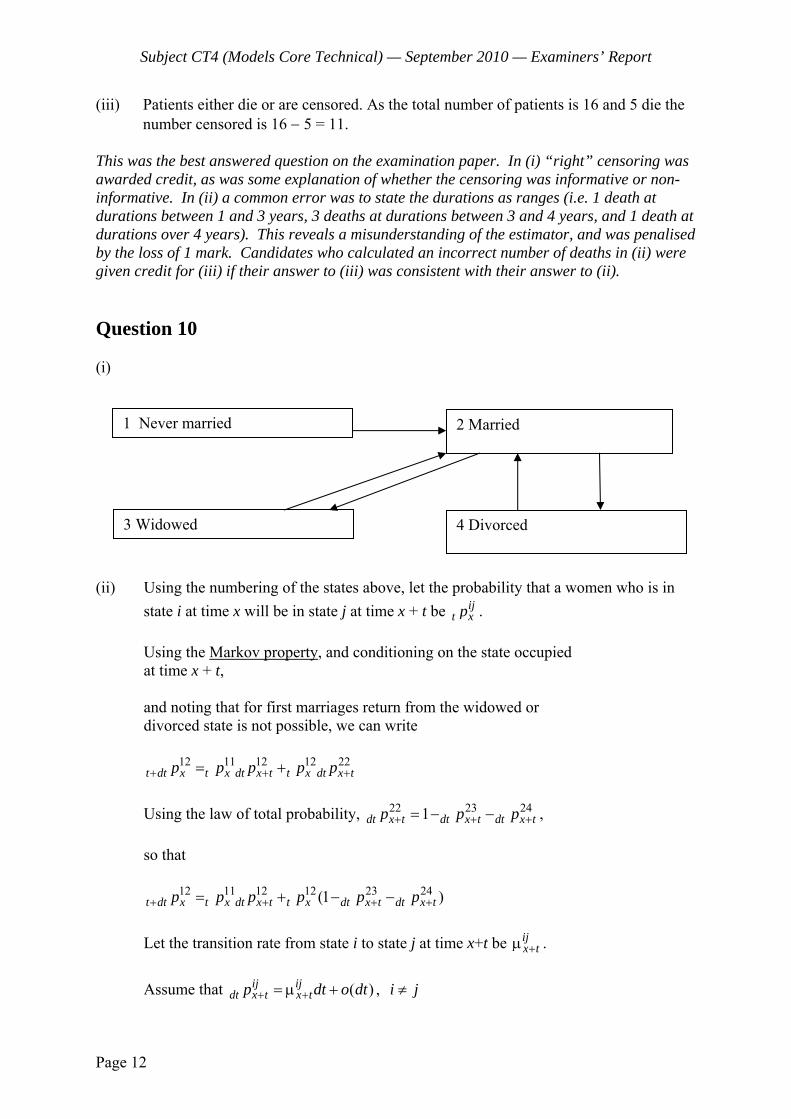
Subject CT4 (Models Core Technical) — September 2010 — Examiners’ Report
Page 12
(iii) Patients either die or are censored. As the total number of patients is 16 and 5 die the number censored is 16 − 5 = 11.
This was the best answered question on the examination paper. In (i) “right” censoring was awarded credit, as was some explanation of whether the censoring was informative or non-informative. In (ii) a common error was to state the durations as ranges (i.e. 1 death at durations between 1 and 3 years, 3 deaths at durations between 3 and 4 years, and 1 death at durations over 4 years). This reveals a misunderstanding of the estimator, and was penalised by the loss of 1 mark. Candidates who calculated an incorrect number of deaths in (ii) were given credit for (iii) if their answer to (iii) was consistent with their answer to (ii). Question 10 (i)
(ii) Using the numbering of the states above, let the probability that a women who is in
state i at time x will be in state j at time x + t be ijt xp .
Using the Markov property, and conditioning on the state occupied at time x + t, and noting that for first marriages return from the widowed or divorced state is not possible, we can write
12 11 12 12 22
t dt x t x dt x t t x dt x tp p p p p+ + += + Using the law of total probability, 22 23 241dt x t dt x t dt x tp p p+ + += − − ,
so that 12 11 12 12 23 24(1 )t dt x t x dt x t t x dt x t dt x tp p p p p p+ + + += + − − Let the transition rate from state i to state j at time x+t be ij
x t+μ . Assume that ( )ij ij
dt x t x tp dt o dt+ += μ + , i j≠
1 Never married 2 Married
4 Divorced 3 Widowed

Subject CT4 (Models Core Technical) — September 2010 — Examiners’ Report
Page 13
where 0
( )lim 0dt
o dtdt+→
= .
Substituting for the ij
t xp in the equation above produces 12 11 12 12 23 24(1 ) ( )t dt x t x x t t x x t x tp p dt p dt dt o dt+ + + += μ + −μ −μ + Therefore 12 12 11 12 12 23 12 24 ( )t dt x t x t x x t t x x t t x x tp p p dt p dt p dt o dt+ + + +− = μ − μ − μ + and, taking limits, we have
12 12
11 12 12 23 12 24
0lim t dt x t x
t x x t t x x t t x x tdt
p p p p pdt
μ μ μ+
++ + +
→
−= − −
So
12 11 12 12 23 12 24t x t x x t t x x t t x x t
d p p p pdt
μ μ μ+ + += − −
(iii) Let the waiting time in state i be vi, and the number of transitions from state i to state j be dij and the transition intensity from state i to state j is ijμ Then the likelihood, L, may be written L = 23 3212 24 42
1 12 2 23 24 3 32 4 42 12 23 24 32 42exp[ ( ) ] d dd d dK v v v v− μ − μ +μ − μ − μ μ μ μ μ μ . (iv) The logarithm of the likelihood is
1 12 2 23 24 3 32 4 42
12 12 23 23 24 24 32 32 42 42
log log ( )log log log log log
e e
e e e e e
L K v v v vd d d d d
= − μ − μ +μ − μ − μ
+ μ + μ + μ + μ + μ
Differentiating with respect to 12μ gives
121
12 12
dL v∂= − +
∂μ μ.

Subject CT4 (Models Core Technical) — September 2010 — Examiners’ Report
Page 14
Setting this equal to 0 and solving for 12μ gives
^
1212
1
dv
μ = .
This is a maximum because 2
122 2
12 12
dL∂= −
∂μ μwhich is negative.
Answers to (i), (iii) and (iv) were generally good. In (i) the arrows from Widowed to Married and Divorced to Married were not required for full marks, as the question is about first marriages. Answers to (ii) were more disappointing, with many candidates omitting steps in the argument. In (ii), some candidates included the extra terms 13 32 14 42
t x x t t x x tp pμ μ+ ++ + . Since it is just about possible to interpret the question in a way such that these should be included, this was not heavily penalised. Question 11 (i) A Markov jump process is a continuous-time Markov process with a discrete state
space.
For a process to be Markov, the future development of the process must depend only on its current state.
This is the case here, as the future of the process depends only on the number of
passengers currently in the front taxi. The number of passengers in the front taxi also has a discrete state space {0, 1, 2, 3}.
(Note that immediately a fourth passenger arrives the taxi will depart so the front taxi in the queue will never have four passengers in it.)
(ii) (a) The generator matrix A is
0 00 00 0
0 0
−β β⎛ ⎞⎜ ⎟−β β⎜ ⎟⎜ ⎟−β β⎜ ⎟β −β⎝ ⎠
(b) Kolmogorov’s forward equations can be written in compact form as
( ) ( )d P t P t Adt
= ,
Which are, for j = 0
0 3 0( ) ( ) ( )i i id p t p t p tdt
= β −β

Subject CT4 (Models Core Technical) — September 2010 — Examiners’ Report
Page 15
and, for j = 1,2,3
, 1( ) ( ) ( )ij i j ijd p t p t p tdt −= β −β .
(iii) Since the waiting times under a Poisson process are exponential the expected waiting
time between the arrival of passengers at the terminus is 1β
minutes.
Successive waiting times are independent, therefore the expected waiting time for a
passenger arriving at the terminus is
3
0
3[ ] ii
iE t p=
−=
β∑ ,
where pi is the probability that the front taxi has exactly i previous passengers waiting
in it when the passenger arrives. Since the pis are all equal for i = 0, 1, 2, 3
3 2 1 0 3[ ] 0.252
E t ⎛ ⎞= + + + =⎜ ⎟β β β β β⎝ ⎠
minutes.
(iv) The transition matrix, P, is
0 1 0 0 00 0 1 0 01 10 0 02 20 0 0 0 11 0 0 0 0
⎛ ⎞⎜ ⎟⎜ ⎟⎜ ⎟⎜ ⎟⎜ ⎟⎜ ⎟⎜ ⎟⎝ ⎠
.
(v) The expected waiting time if the front taxi is a three-passenger model is
2
0
2 1 2 1 0 1[ | 3 passenger model]3i
i
iE t p=
⎛ ⎞−− = = + + =⎜ ⎟β β β β β⎝ ⎠
∑
The expected waiting time if the front taxi is a five-passenger model is
4
0
4 1 4 3 2 1 0 2[ | 5 passenger model]5i
i
iE t p=
⎛ ⎞−− = = + + + + =⎜ ⎟β β β β β β β⎝ ⎠
∑ .
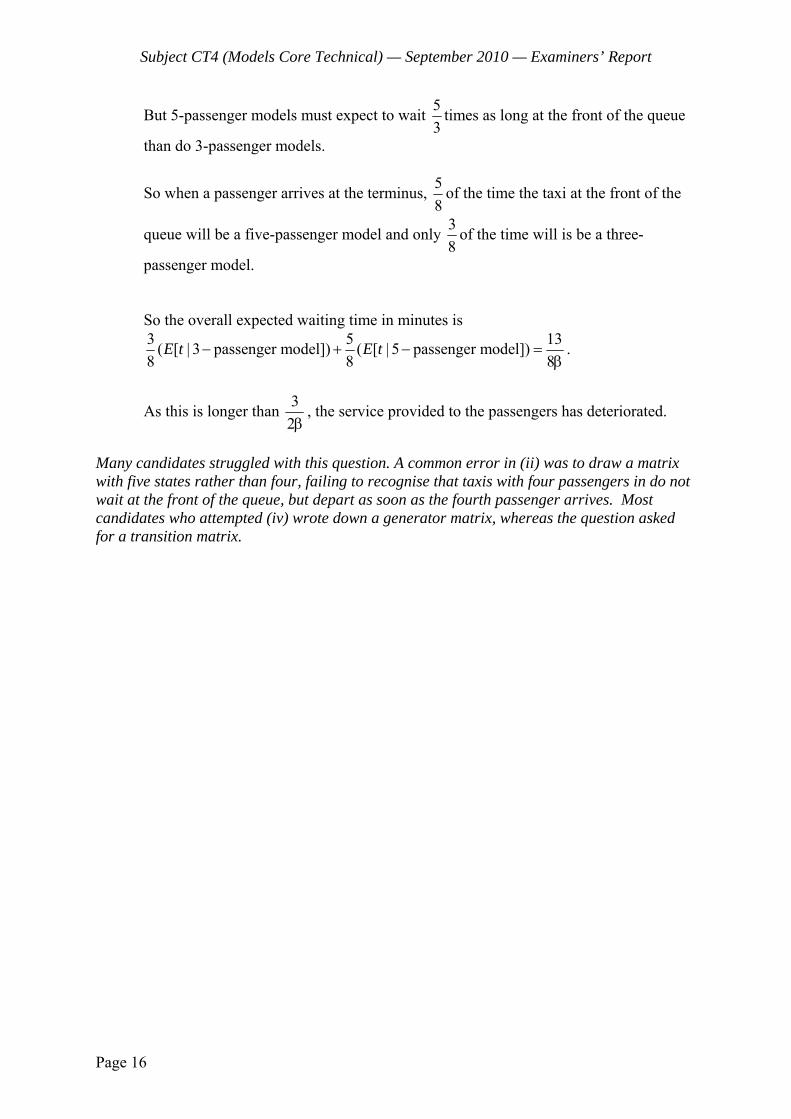
Subject CT4 (Models Core Technical) — September 2010 — Examiners’ Report
Page 16
But 5-passenger models must expect to wait 53
times as long at the front of the queue
than do 3-passenger models.
So when a passenger arrives at the terminus, 58
of the time the taxi at the front of the
queue will be a five-passenger model and only 38
of the time will is be a three-
passenger model.
So the overall expected waiting time in minutes is
3 5 13( [ | 3 passenger model]) ( [ | 5 passenger model])8 8 8
E t E t− + − =β
.
As this is longer than 32β
, the service provided to the passengers has deteriorated.
Many candidates struggled with this question. A common error in (ii) was to draw a matrix with five states rather than four, failing to recognise that taxis with four passengers in do not wait at the front of the queue, but depart as soon as the fourth passenger arrives. Most candidates who attempted (iv) wrote down a generator matrix, whereas the question asked for a transition matrix.
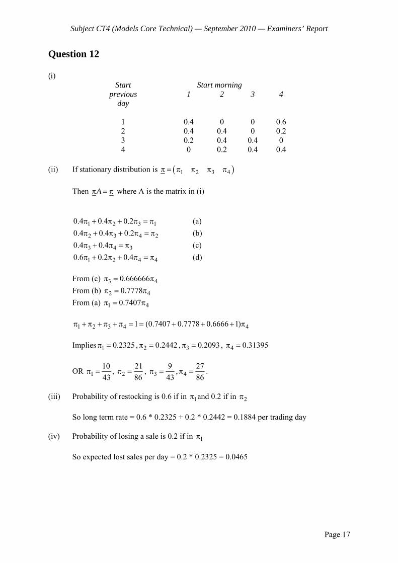
Subject CT4 (Models Core Technical) — September 2010 — Examiners’ Report
Page 17
Question 12 (i)
Start previous
day
Start morning 1 2
3 4
1 0.4 0 0 0.6 2 0.4 0.4 0 0.2 3 0.2 0.4 0.4 0 4 0 0.2 0.4 0.4
(ii) If stationary distribution is ( )1 2 3 4π = π π π π Then Aπ = π where A is the matrix in (i)
1 2 3 10.4 0.4 0.2π + π + π = π (a) 2 3 4 20.4 0.4 0.2π + π + π = π (b) 3 4 30.4 0.4π + π = π (c) 1 2 4 40.6 0.2 0.4π + π + π = π (d)
From (c) 3 40.666666π = π From (b) 2 40.7778π = π From (a) 1 40.7407π = π 1 2 3 4 41 (0.7407 0.7778 0.6666 1)π + π + π + π = = + + + π
Implies 1 0.2325π = , 2 0.2442π = , 3 0.2093π = , 4 0.31395π =
OR 11043
π = , 22186
π = , 3943
π = , 42786
π = .
(iii) Probability of restocking is 0.6 if in 1π and 0.2 if in 2π So long term rate = 0.6 * 0.2325 + 0.2 * 0.2442 = 0.1884 per trading day
(iv) Probability of losing a sale is 0.2 if in 1π So expected lost sales per day = 0.2 * 0.2325 = 0.0465
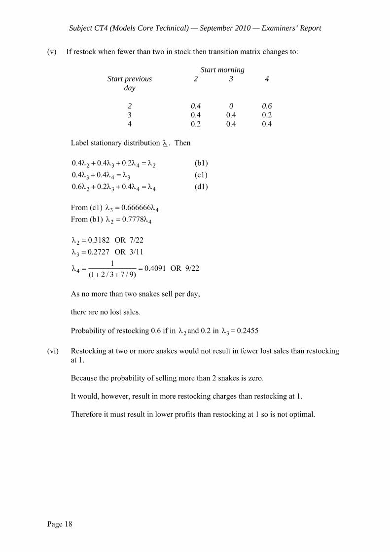
Subject CT4 (Models Core Technical) — September 2010 — Examiners’ Report
Page 18
(v) If restock when fewer than two in stock then transition matrix changes to:
Start previous
day
Start morning 2 3 4
2 0.4 0 0.6 3 0.4 0.4 0.2 4 0.2 0.4 0.4
Label stationary distribution λ . Then 2 3 4 20.4 0.4 0.2λ + λ + λ = λ (b1) 3 4 30.4 0.4λ + λ = λ (c1) 2 3 4 40.6 0.2 0.4λ + λ + λ = λ (d1)
From (c1) 3 40.666666λ = λ From (b1) 2 40.7778λ = λ
2 0.3182λ = OR 7/22 3 0.2727λ = OR 3/11
41 0.4091
(1 2 / 3 7 / 9)λ = =
+ + OR 9/22
As no more than two snakes sell per day, there are no lost sales.
Probability of restocking 0.6 if in 2λ and 0.2 in 3λ = 0.2455
(vi) Restocking at two or more snakes would not result in fewer lost sales than restocking
at 1. Because the probability of selling more than 2 snakes is zero. It would, however, result in more restocking charges than restocking at 1.
Therefore it must result in lower profits than restocking at 1 so is not optimal.

Subject CT4 (Models Core Technical) — September 2010 — Examiners’ Report
Page 19
(vii) Costs if restock at 0 0.1884C + 0.0465P Costs if restock at 1 0.24546C
So should change restocking approach if 0.24546C < 0.1884C + 0.0465P C < 0.8148P In this question, many candidates answered (i) and (ii), but made no further progress. Candidates who wrote down the wrong matrix in (i) but evaluated the stationary distribution correctly for the matrix they had written down were given full credit for (ii), and gained credit in (iii) and (iv) if these parts were answered correctly given the matrix which had been written down in (i). A common error was to write down a five-state model in (i). Few candidates attempted the later sections of this question.
END OF EXAMINERS’ REPORT

INSTITUTE AND FACULTY OF ACTUARIES
EXAMINATION
15 April 2011 (am)
Subject CT4 — Models Core Technical
Time allowed: Three hours
INSTRUCTIONS TO THE CANDIDATE
1. Enter all the candidate and examination details as requested on the front of your answer booklet.
2. You must not start writing your answers in the booklet until instructed to do so by the
supervisor. 3. Mark allocations are shown in brackets. 4. Attempt all 12 questions, beginning your answer to each question on a separate sheet. 5. Candidates should show calculations where this is appropriate.
Graph paper is NOT required for this paper.
AT THE END OF THE EXAMINATION
Hand in BOTH your answer booklet, with any additional sheets firmly attached, and this question paper.
In addition to this paper you should have available the 2002 edition of the Formulae and Tables and your own electronic calculator from the approved list.
CT4 A2011 © Institute and Faculty of Actuaries

CT4 A2011—2
1 Give three advantages of the two-state model over the Binomial model for estimating transition intensities where exact dates of entry into and exit from observation are known. [3]
2 Distinguish between the conditions under which a Markov chain:
(a) has at least one stationary distribution. (b) has a unique stationary distribution. (c) converges to a unique stationary distribution. [3]
3 Describe the ways in which the design of a model used to project over only a short time frame may differ from one used to project over fifty years. [4]
4 Children at a school are given weekly grade sheets, in which their effort is graded in
four levels: 1 “Poor”, 2 “Satisfactory”, 3 “Good” and 4 “Excellent”. Subject to a maximum level of Excellent and a minimum level of Poor, between each week and the next, a child has:
• a 20 per cent chance of moving up one level. • a 20 per cent chance of moving down one level. • a 10 per cent chance of moving up two levels. • a 10 per cent chance of moving down two levels.
Moving up or down three levels in a single week is not possible. (i) Write down the transition matrix of this process. [2] Children are graded on Friday afternoon in each week. On Friday of the first week of
the school year, as there is little evidence on which to base an assessment, all children are graded “Satisfactory”.
(ii) Calculate the probability distribution of the process after the grading on Friday
of the third week of the school year. [3] [Total 5]

CT4 A2011—3 PLEASE TURN OVER
5 (i) Explain why a mortality experience would need to be graduated. [3] An actuary has conducted investigations into the mortality of the following classes of
lives:
(a) the female members of a medium-sized pension scheme
(b) the male population of a large industrial country
(c) the population of a particular species of reptile in the zoological collections of the southern hemisphere
The actuary wishes to graduate the crude rates. (ii) State an appropriate method of graduation for each of the three classes of lives
and, for each class, briefly explain your choice. [3] [Total 6] 6 A study of the mortality of a certain species of insect reveals that for the first 30 days
of life, the insects are subject to a constant force of mortality of 0.05. After 30 days, the force of mortality increases according to the formula:
30 0.05exp(0.01 )x x+μ = ,
where x is the number of days after day 30.
(i) Calculate the probability that a newly born insect will survive for at least 10 days. [1]
(ii) Calculate the probability that an insect aged 10 days will survive for at least a
further 30 days. [3] (iii) Calculate the age in days by which 90 per cent of insects are expected to have
died. [4] [Total 8] 7 (i) Define a counting process. [2] For each of the following processes:
• simple random walk • compound Poisson • Markov chain
(ii) (a) State whether each of the state space and the time set is discrete,
continuous or can be either. (b) Give an example of an application which may be useful to a
shopkeeper selling dried fruit and nuts loose. [6] [Total 8]
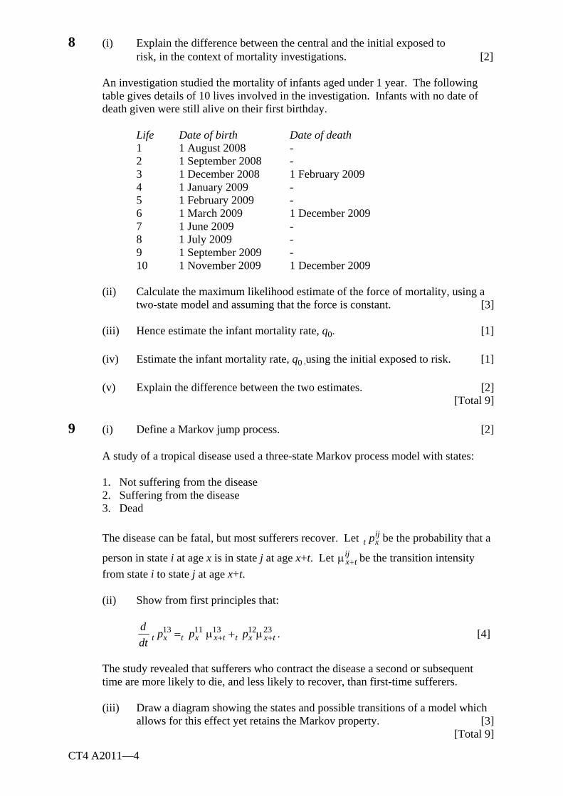
CT4 A2011—4
8 (i) Explain the difference between the central and the initial exposed to risk, in the context of mortality investigations. [2]
An investigation studied the mortality of infants aged under 1 year. The following table gives details of 10 lives involved in the investigation. Infants with no date of death given were still alive on their first birthday.
Life Date of birth Date of death 1 1 August 2008 - 2 1 September 2008 - 3 1 December 2008 1 February 2009 4 1 January 2009 - 5 1 February 2009 - 6 1 March 2009 1 December 2009 7 1 June 2009 - 8 1 July 2009 - 9 1 September 2009 - 10 1 November 2009 1 December 2009
(ii) Calculate the maximum likelihood estimate of the force of mortality, using a
two-state model and assuming that the force is constant. [3] (iii) Hence estimate the infant mortality rate, q0. [1] (iv) Estimate the infant mortality rate, q0 ,using the initial exposed to risk. [1] (v) Explain the difference between the two estimates. [2]
[Total 9] 9 (i) Define a Markov jump process. [2] A study of a tropical disease used a three-state Markov process model with states:
1. Not suffering from the disease 2. Suffering from the disease 3. Dead
The disease can be fatal, but most sufferers recover. Let ijt xp be the probability that a
person in state i at age x is in state j at age x+t. Let ijx t+μ be the transition intensity
from state i to state j at age x+t.
(ii) Show from first principles that:
13 11 13 12 23t x t x x t t x x t
d p p pdt + += μ + μ . [4]
The study revealed that sufferers who contract the disease a second or subsequent
time are more likely to die, and less likely to recover, than first-time sufferers. (iii) Draw a diagram showing the states and possible transitions of a model which
allows for this effect yet retains the Markov property. [3] [Total 9]

CT4 A2011—5 PLEASE TURN OVER
10 At Miracle Cure hospital a pioneering new surgery was tested to replace human lungs with synthetic implants. Operations were carried out throughout June 2010. Patients who underwent the surgery were monitored daily until the end of August 2010, or until they died or left hospital if sooner. The results are shown below. Where no date is given, the patient was alive and still in hospital at the end of August.
Patient Date of surgery Date of leaving observation
Reason for leaving
observation
A B C D E F G H I J K L M N
June 1 June 3 June 5 June 8 June 9 June 12 June 16 June 17 June 22 June 24 June 25 June 26 June 29 June 30
June 3 July 2
July 11
June 21 Aug 12
June 29 Aug 20
Aug 6
Died Left Hospital
Died
Died Left Hospital
Died Died
Left Hospital
(i) Explain whether each of the following types of censoring is present and for
those present explain where they occur:
• right censoring • left censoring • informative censoring
[3]
(ii) Calculate the Kaplan-Meier estimate of the survival function for these patients, stating all assumptions that you make. [6]
(iii) Sketch, on a suitably labelled graph, the Kaplan-Meier estimate of the survival
function. [2] (iv) Estimate the probability that a patient will die within four weeks of surgery. [1] [Total 12]
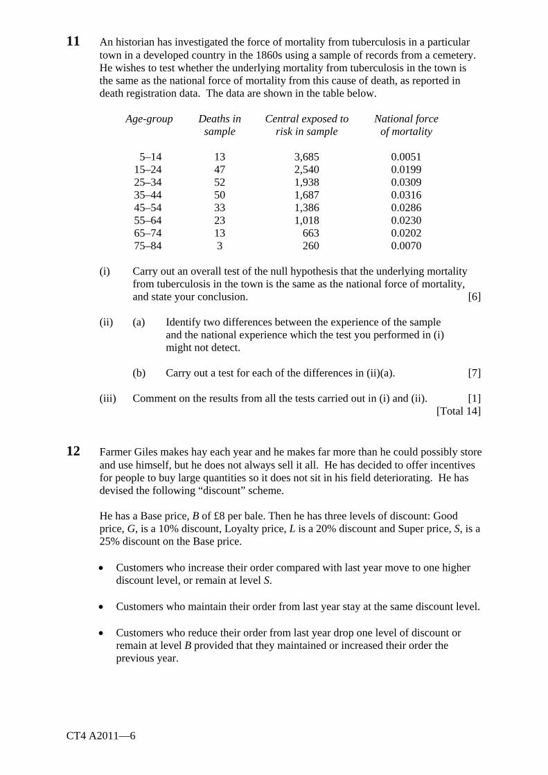
CT4 A2011—6
11 An historian has investigated the force of mortality from tuberculosis in a particular town in a developed country in the 1860s using a sample of records from a cemetery. He wishes to test whether the underlying mortality from tuberculosis in the town is the same as the national force of mortality from this cause of death, as reported in death registration data. The data are shown in the table below.
Age-group Deaths in Central exposed to National force
sample risk in sample of mortality
5–14 13 3,685 0.0051 15–24 47 2,540 0.0199 25–34 52 1,938 0.0309 35–44 50 1,687 0.0316 45–54 33 1,386 0.0286 55–64 23 1,018 0.0230 65–74 13 663 0.0202 75–84 3 260 0.0070
(i) Carry out an overall test of the null hypothesis that the underlying mortality
from tuberculosis in the town is the same as the national force of mortality, and state your conclusion. [6]
(ii) (a) Identify two differences between the experience of the sample
and the national experience which the test you performed in (i) might not detect.
(b) Carry out a test for each of the differences in (ii)(a). [7]
(iii) Comment on the results from all the tests carried out in (i) and (ii). [1]
[Total 14]
12 Farmer Giles makes hay each year and he makes far more than he could possibly store and use himself, but he does not always sell it all. He has decided to offer incentives for people to buy large quantities so it does not sit in his field deteriorating. He has devised the following “discount” scheme.
He has a Base price, B of £8 per bale. Then he has three levels of discount: Good price, G, is a 10% discount, Loyalty price, L is a 20% discount and Super price, S, is a 25% discount on the Base price. • Customers who increase their order compared with last year move to one higher
discount level, or remain at level S.
• Customers who maintain their order from last year stay at the same discount level.
• Customers who reduce their order from last year drop one level of discount or remain at level B provided that they maintained or increased their order the previous year.

CT4 A2011—7
• Customers who reduce their order from last year drop two levels of discount if they also reduced their order last year, subject to remaining at the lowest level B.
(i) Explain why a process with the state space of {B, G, L, S} does not display the
Markov property. [2]
(ii) (a) Define any additional state(s) required to model the system with the Markov property.
(b) Construct a transition graph of this Markov process clearly labelling all the states. [3]
Farmer Giles thinks that each year customers have a 60% likelihood of increasing their order and a 30% likelihood of reducing it, irrespective of the discount level they are currently in.
(iii) (a) Write down the transition matrix for the Markov process. (b) Calculate the stationary distribution. (c) Hence calculate the long run average price he will get for each bale of
hay. [8]
(iv) Calculate the probability that a customer who is currently paying the Loyalty
price, L, will be paying L in two years’ time. [3] (v) Suggest reasons why the assumptions Farmer Giles has made about his
customers’ behaviour may not be valid. [3] [Total 19]
END OF PAPER

INSTITUTE AND FACULTY OF ACTUARIES
EXAMINERS’ REPORT
April 2011 examinations
Subject CT4 — Models Core Technical
Introduction The attached subject report has been written by the Principal Examiner with the aim of helping candidates. The questions and comments are based around Core Reading as the interpretation of the syllabus to which the examiners are working. They have however given credit for any alternative approach or interpretation which they consider to be reasonable. T J Birse Chairman of the Board of Examiners July 2011
© Institute and Faculty of Actuaries

Subject CT4 (Models Core Technical) — Examiners’ Report, April 2011
Page 2
Question 1 We can calculate the maximum likelihood estimate (MLE) of the transition intensities directly using the two-state model, whereas the Binomial model requires additional assumptions. The variance of the Binomial estimate is greater than that of the estimate from the two-state model (though the difference is tiny unless the transition intensities are large). The MLE in the two-state model is consistent and unbiased, whereas the Binomial estimate is only consistent and unbiased if lives are observed for exactly one year, which is rarely the case. The two-state model is easily extended to encompass increments and additional decrements, whereas the Binomial model is not. The two-state model uses the exact times of the transitions, whereas the Binomial model only uses the number of transitions. This question was poorly answered by many candidates, despite being straightforward bookwork. Many candidates commented that the two-state model and the Binomial model make different assumptions about the shape of the force of mortality within the year of age. This was only be given credit if candidates also explained why the multiple state model’s assumption is BETTER than the Binomial model’s assumption (which it might be, for example, at younger ages). Full marks could be obtained for giving three reasons. It was not necessary to give all the points listed above in order to obtain full marks. Question 2 (a) A Markov chain with a finite state space has at least one stationary probability
distribution. (b) An irreducible Markov chain with a finite state space has a unique stationary
probability distribution. (c) A Markov chain with a finite state space which is irreducible, and which is also
aperiodic converges to a unique stationary probability distribution. Many candidates scored full marks on this question. The question asked candidates to “distinguish”. Therefore for full credit it is important that candidates did, indeed, understand and make the relevant distinction.

Subject CT4 (Models Core Technical) — Examiners’ Report, April 2011
Page 3
Question 3 Individual variables may behave differently, for example a model over 50 years may be more sensitive to differences in the input values of certain variables than one over the short term. A variable which has an ignorable effect in the short term may have a non-ignorable effect over 50 years.
Over the short term, it may be reasonable to assume the values of some variables to be constant or to vary linearly, whereas this would not be reasonable over 50 years. For example, growth which is exponential may appear linear if studied over a short time frame. The interaction between variables in the short-term may be different from that over the long-term.
Higher order relationships between variables may be ignored for simplicity if modelling over a short time frame. The time units used in the model might be shorter for a model projecting over a short time frame, so that the total number of time units used in each model is roughly the same. Over 50 years, regulatory changes and other “shock” events are more likely to occur, and the model design may need to consider the circumstances in which the results or conclusions may be materially impacted (e.g. in the short term the tax basis may be known, but in the long run it is likely to change).
The marks on this question were the lowest on any question. The question was a “higher skills” question and so required candidates to think about the context. Little credit was given to candidates who uncritically reproduced sections of the Core Reading. In particular, the question is about model DESIGN, so the points made should relate to the design of the model.
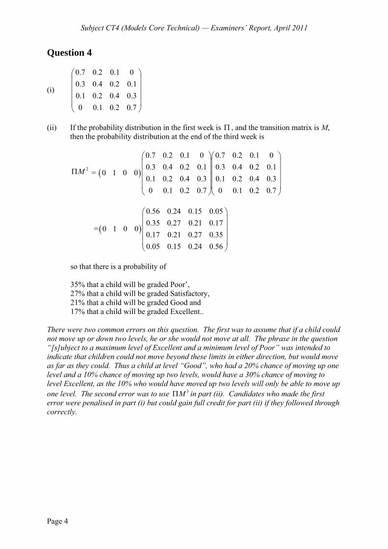
Subject CT4 (Models Core Technical) — Examiners’ Report, April 2011
Page 4
Question 4
(i)
0.7 0.2 0.1 00.3 0.4 0.2 0.10.1 0.2 0.4 0.30 0.1 0.2 0.7
⎛ ⎞⎜ ⎟⎜ ⎟⎜ ⎟⎜ ⎟⎝ ⎠
(ii) If the probability distribution in the first week is Π , and the transition matrix is M,
then the probability distribution at the end of the third week is
2MΠ = ( )
0.7 0.2 0.1 0 0.7 0.2 0.1 00.3 0.4 0.2 0.1 0.3 0.4 0.2 0.1
0 1 0 00.1 0.2 0.4 0.3 0.1 0.2 0.4 0.30 0.1 0.2 0.7 0 0.1 0.2 0.7
⎛ ⎞⎛ ⎞⎜ ⎟⎜ ⎟⎜ ⎟⎜ ⎟⎜ ⎟⎜ ⎟⎜ ⎟⎜ ⎟⎝ ⎠⎝ ⎠
= ( )
0.56 0.24 0.15 0.050.35 0.27 0.21 0.17
0 1 0 00.17 0.21 0.27 0.350.05 0.15 0.24 0.56
⎛ ⎞⎜ ⎟⎜ ⎟⎜ ⎟⎜ ⎟⎝ ⎠
so that there is a probability of 35% that a child will be graded Poor’, 27% that a child will be graded Satisfactory, 21% that a child will be graded Good and 17% that a child will be graded Excellent.. There were two common errors on this question. The first was to assume that if a child could not move up or down two levels, he or she would not move at all. The phrase in the question “[s]ubject to a maximum level of Excellent and a minimum level of Poor” was intended to indicate that children could not move beyond these limits in either direction, but would move as far as they could. Thus a child at level “Good”, who had a 20% chance of moving up one level and a 10% chance of moving up two levels, would have a 30% chance of moving to level Excellent, as the 10% who would have moved up two levels will only be able to move up one level. The second error was to use 3MΠ in part (ii). Candidates who made the first error were penalised in part (i) but could gain full credit for part (ii) if they followed through correctly.
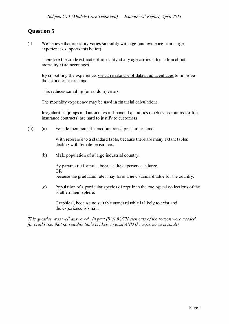
Subject CT4 (Models Core Technical) — Examiners’ Report, April 2011
Page 5
Question 5 (i) We believe that mortality varies smoothly with age (and evidence from large experiences supports this belief).
Therefore the crude estimate of mortality at any age carries information about
mortality at adjacent ages.
By smoothing the experience, we can make use of data at adjacent ages to improve the estimates at each age.
This reduces sampling (or random) errors.
The mortality experience may be used in financial calculations.
Irregularities, jumps and anomalies in financial quantities (such as premiums for life
insurance contracts) are hard to justify to customers.
(ii) (a) Female members of a medium-sized pension scheme.
With reference to a standard table, because there are many extant tables dealing with female pensioners.
(b) Male population of a large industrial country. By parametric formula, because the experience is large. OR because the graduated rates may form a new standard table for the country. (c) Population of a particular species of reptile in the zoological collections of the
southern hemisphere. Graphical, because no suitable standard table is likely to exist and the experience is small.
This question was well answered. In part (i)(c) BOTH elements of the reason were needed for credit (i.e. that no suitable table is likely to exist AND the experience is small).
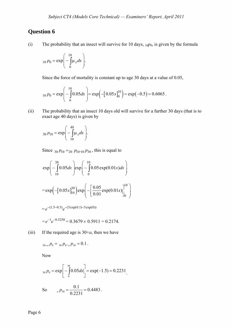
Subject CT4 (Models Core Technical) — Examiners’ Report, April 2011
Page 6
Question 6 (i) The probability that an insect will survive for 10 days, 10p0, is given by the formula
10
10 00
exp xp dx⎛ ⎞⎜ ⎟= − μ⎜ ⎟⎝ ⎠∫ .
Since the force of mortality is constant up to age 30 days at a value of 0.05,
[ ]( ) ( )10
1010 0 0
0
exp 0.05 exp 0.05 exp 0.5 0.6065p dx x⎛ ⎞⎜ ⎟= − = − = − =⎜ ⎟⎝ ⎠∫ .
(ii) The probability that an insect 10 days old will survive for a further 30 days (that is to exact age 40 days) is given by
40
30 1010
exp xp dx⎛ ⎞⎜ ⎟= − μ⎜ ⎟⎝ ⎠∫ .
Since 30 10 20 10 10 30.p p p= , this is equal to
30 10
10 0
exp 0.05 exp 0.05exp(0.01 )dx x dx⎛ ⎞ ⎛ ⎞⎜ ⎟ ⎜ ⎟− −⎜ ⎟ ⎜ ⎟⎝ ⎠ ⎝ ⎠∫ ∫
= [ ]( )10
3010
0
0.05exp 0.05 exp exp(0.01 )0.01
x x⎛ ⎞⎡ ⎤⎜ ⎟− − ⎢ ⎥⎜ ⎟⎣ ⎦⎝ ⎠
= (1.5 0.5) (5exp(0.1) 5exp(0))e e− − − −
= 1 0.5258e e− − = 0.3679 × 0.5911 = 0.2174. (iii) If the required age is 30+a, then we have
30 0 30 0 30. 0.1a ap p p+ = = . Now
30
30 00
exp 0.05 exp( 1.5) 0.2231p dx⎡ ⎤
= − = − =⎢ ⎥⎣ ⎦∫ .
So 300.1 0.4483
0.2231a p = = .
Subject CT4 (Models Core Technical) — Examiners’ Report, April 2011
Page 7
Using the result from part (ii), we have
0.01 0.01 0.0130
0
0.05 0.05 0.05exp exp exp(5 5 )0.01 0.01 0.01
ax a a
a p e e e⎛ ⎞ ⎛ ⎞⎡ ⎤ ⎡ ⎤= − = − − = −⎜ ⎟ ⎜ ⎟⎢ ⎥ ⎢ ⎥⎜ ⎟⎣ ⎦ ⎣ ⎦⎝ ⎠⎝ ⎠
Therefore 5(1 exp(0.01 )) 0.4483ae − = , whence 0.01log 0.4483 5(1 )a
e e= − ,
so that
0.01
0.01
1 0.16051.1605
0.01 0.148814.88
a
a
ee
aa
− = −
==
=
Therefore the required age is 14.88+30 = 44.88 days. Most candidates answered part (i) of this question correctly. Part (ii) was less well answered, and only a minority of candidates managed to obtain the correct answer to part (iii). A common error was to use the limits 40 and 30 when integrating 0.05exp(0.01x). Question 7 (i) It is a stochastic process in discrete or continuous time. The state space is all the natural numbers {0, 1, 2, ... }
The value of the process X(t) is a non-decreasing (OR an increasing) function of time t
OR the value of the process goes up one at a time. (ii) (a) Process State space Time set
Simple random walk Discrete Discrete Compound Poisson process Either Continuous Markov Chain Discrete Discrete
Subject CT4 (Models Core Technical) — Examiners’ Report, April 2011
Page 8
(b) Process Application
Simple random walk The number of customers in the shop each time the door is opened
Compound Poisson process The weight of almonds remaining in
stock at any time in the day. OR
value of goods sold at any time during the day
Markov chain The number of customers owning loyalty cards at the end of each week. In part (i), it was not sufficient just to say “discrete state space”. The fact the state space is all natural numbers should be indicated for credit. In part (ii)(B), some candidates only gave one example IN TOTAL, whereas the question asked for an example FOR EACH PROCESS. In part (ii)(b) other examples were given credit. The criterion used to award credit were whether the example COULD be modelled using the relevant process and how USEFUL to the shopkeeper such a model might be! Question 8 (i) EITHER The central exposed to risk at age x, c
xE , is the waiting time in a multiple-state or Poisson model. The initial exposed to risk is equal to the central exposed to risk plus the time elapsing
between the date of death and the end of the rate interval for those who are observed to die during the rate interval.
OR
If the age at entry of life i is x + ai , and the age at exit is x+bi for lives which do not die, and x+ti for lives who die, then the central exposed to risk is equal to [( ) ( )] ( )i i i i i i
i ix b x a b a+ − − = −∑ ∑ for lives who do not die, and
[( ) ( )] ( )i i i i i ii i
x t x a t a+ − − = −∑ ∑ for lives who die.
The initial exposed to risk is given by the central exposed to risk plus a quantity equal to (1 )i
it−∑ for the lives who die.
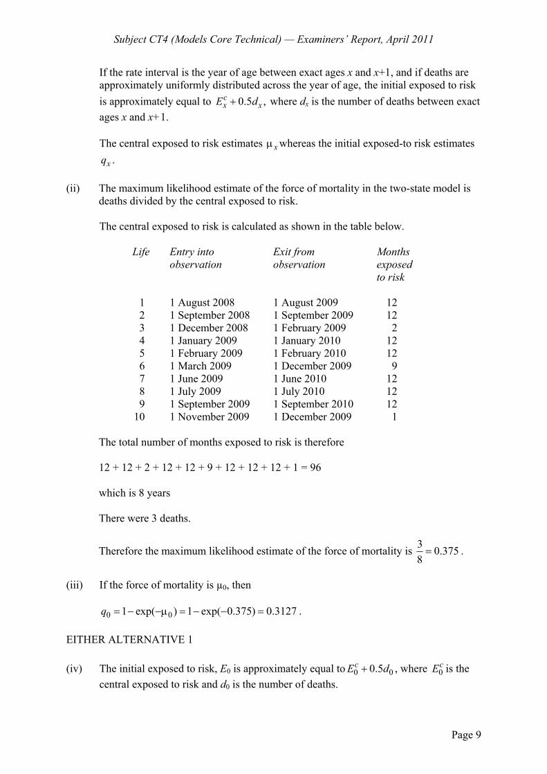
Subject CT4 (Models Core Technical) — Examiners’ Report, April 2011
Page 9
If the rate interval is the year of age between exact ages x and x+1, and if deaths are approximately uniformly distributed across the year of age, the initial exposed to risk is approximately equal to 0.5 ,c
x xE d+ where dx is the number of deaths between exact ages x and x+1.
The central exposed to risk estimates xμ whereas the initial exposed-to risk estimates
xq .
(ii) The maximum likelihood estimate of the force of mortality in the two-state model is deaths divided by the central exposed to risk.
The central exposed to risk is calculated as shown in the table below.
Life Entry into Exit from Months observation observation exposed to risk
1 1 August 2008 1 August 2009 12
2 1 September 2008 1 September 2009 12 3 1 December 2008 1 February 2009 2 4 1 January 2009 1 January 2010 12 5 1 February 2009 1 February 2010 12 6 1 March 2009 1 December 2009 9 7 1 June 2009 1 June 2010 12 8 1 July 2009 1 July 2010 12 9 1 September 2009 1 September 2010 12 10 1 November 2009 1 December 2009 1
The total number of months exposed to risk is therefore
12 + 12 + 2 + 12 + 12 + 9 + 12 + 12 + 12 + 1 = 96
which is 8 years
There were 3 deaths.
Therefore the maximum likelihood estimate of the force of mortality is 3 0.3758= .
(iii) If the force of mortality is µ0, then 0 01 exp( ) 1 exp( 0.375) 0.3127q = − −μ = − − = . EITHER ALTERNATIVE 1 (iv) The initial exposed to risk, E0 is approximately equal to 0 00.5cE d+ , where 0
cE is the central exposed to risk and d0 is the number of deaths.
Subject CT4 (Models Core Technical) — Examiners’ Report, April 2011
Page 10
Therefore we have
00
0 0
3 3* 0.31588 0.5(3) 9.50.5c
dqE d
= = = =++
.
(v) 0 *q is calculated assuming a uniform distribution of deaths over the year of age between birth and exact age 1 year, whereas 0q assumes a constant force of mortality between exact ages 0 and 1. These assumptions are different, implying a different distribution of deaths over the first year of life. OR ALTERNATIVE 2
(iv) As the only way of leaving observation is through death, the initial exposed to risk is 10
and 03* 0.3
10q = = .
(v) 0 *q is calculated using the exact initial exposed to risk, making no assumptions about the shape of the force of mortality during the interval, OR
In the calculation of 0 *q lives could die at any time during the year of age, so they are treated as being exposed to risk for the entire year, whereas 0q assumes a constant force of mortality between exact ages 0 and 1, which implies an assumption about the distribution of deaths over this interval.
In part (i) full credit could be obtained for rather less than is written in the solution above. Credit can be given for any clear algebraic expressions in terms of the entry age x+ai , the age at death, x+ti and the age at exit if the life did not die, x+bi, which made clear the difference between the central and initial exposeds to risk. In part (v) the wording did not have to be precise. The Examiners were looking for some understanding of the idea that different assumptions are made about the shape of the force of mortality over the rate interval.
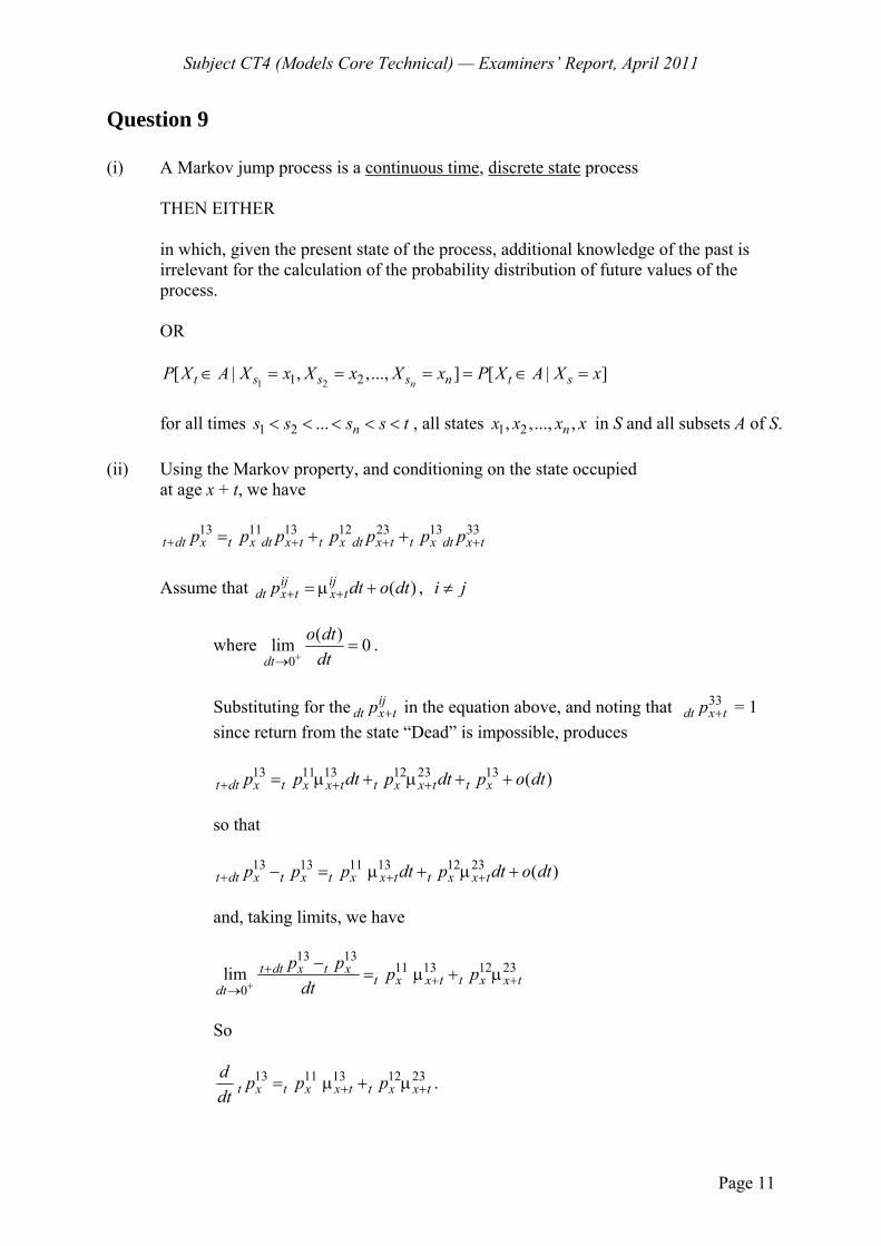
Subject CT4 (Models Core Technical) — Examiners’ Report, April 2011
Page 11
Question 9 (i) A Markov jump process is a continuous time, discrete state process THEN EITHER in which, given the present state of the process, additional knowledge of the past is irrelevant for the calculation of the probability distribution of future values of the process. OR
1 21 2[ | , ,..., ] [ | ]nt s s s n t sP X A X x X x X x P X A X x∈ = = = = ∈ =
for all times 1 2 ... ns s s s t< < < < < , all states 1 2, ,..., ,nx x x x in S and all subsets A of S. (ii) Using the Markov property, and conditioning on the state occupied at age x + t, we have 13 11 13 12 23 13 33
t dt x t x dt x t t x dt x t t x dt x tp p p p p p p+ + + += + + Assume that ( )ij ij
dt x t x tp dt o dt+ += μ + , i j≠
where 0
( )lim 0dt
o dtdt+→
= .
Substituting for the ij
dt x tp + in the equation above, and noting that 33dt x tp + = 1
since return from the state “Dead” is impossible, produces 13 11 13 12 23 13 ( )t dt x t x x t t x x t t xp p dt p dt p o dt+ + += μ + μ + + so that 13 13 11 13 12 23 ( )t dt x t x t x x t t x x tp p p dt p dt o dt+ + +− = μ + μ + and, taking limits, we have
13 13
11 13 12 23
0lim t dt x t x
t x x t t x x tdt
p p p pdt+
++ +
→
−= μ + μ
So
13 11 13 12 23t x t x x t t x x t
d p p pdt + += μ + μ .
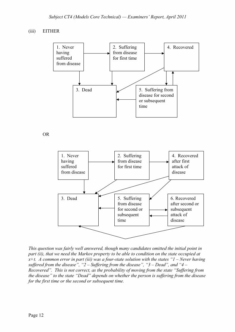
Subject CT4 (Models Core Technical) — Examiners’ Report, April 2011
Page 12
(iii) EITHER
OR
This question was fairly well answered, though many candidates omitted the initial point in part (ii), that we need the Markov property to be able to condition on the state occupied at x+t. A common error in part (iii) was a four-state solution with the states “1 – Never having suffered from the disease”, “2 – Suffering from the disease”, “3 – Dead”, and “4 – Recovered”. This is not correct, as the probability of moving from the state “Suffering from the disease” to the state “Dead” depends on whether the person is suffering from the disease for the first time or the second or subsequent time.
1. Never having suffered from disease
2. Suffering from disease for first time
4. Recovered
3. Dead 5. Suffering from disease for second or subsequent time
1. Never having suffered from disease
2. Suffering from disease for first time
4. Recovered after first attack of disease
3. Dead 5. Suffering from disease for second or subsequent time
6. Recovered after second or subsequent attack of disease
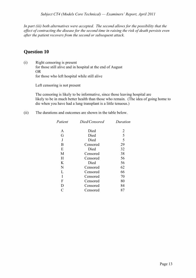
Subject CT4 (Models Core Technical) — Examiners’ Report, April 2011
Page 13
In part (iii) both alternatives were accepted. The second allows for the possibility that the effect of contracting the disease for the second time in raising the risk of death persists even after the patient recovers from the second or subsequent attack. Question 10 (i) Right censoring is present
for those still alive and in hospital at the end of August OR for those who left hospital while still alive Left censoring is not present The censoring is likely to be informative, since those leaving hospital are likely to be in much better health than those who remain. (The idea of going home to die when you have had a lung transplant is a little tenuous.)
(ii) The durations and outcomes are shown in the table below. Patient Died/Censored Duration A Died 2 G Died 5
J Died 5 B Censored 29 E Died 32 M Censored 38 H Censored 56 K Died 56 N Censored 62 L Censored 66 I Censored 70 F Censored 80 D Censored 84 C Censored 87
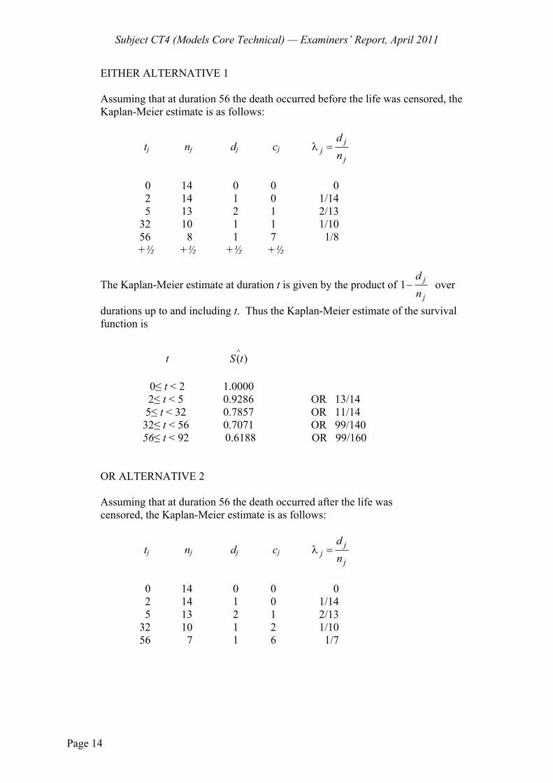
Subject CT4 (Models Core Technical) — Examiners’ Report, April 2011
Page 14
EITHER ALTERNATIVE 1 Assuming that at duration 56 the death occurred before the life was censored, the Kaplan-Meier estimate is as follows:
tj nj dj cj j
jj
dn
λ =
0 14 0 0 0 2 14 1 0 1/14 5 13 2 1 2/13 32 10 1 1 1/10 56 8 1 7 1/8 +½ +½ +½ +½
The Kaplan-Meier estimate at duration t is given by the product of 1 j
j
dn
− over
durations up to and including t. Thus the Kaplan-Meier estimate of the survival function is
t ^( )S t 0≤ t < 2 1.0000 2≤ t < 5 0.9286 OR 13/14 5≤ t < 32 0.7857 OR 11/14 32≤ t < 56 0.7071 OR 99/140 56≤ t < 92 0.6188 OR 99/160 OR ALTERNATIVE 2 Assuming that at duration 56 the death occurred after the life was
censored, the Kaplan-Meier estimate is as follows:
tj nj dj cj j
jj
dn
λ =
0 14 0 0 0 2 14 1 0 1/14 5 13 2 1 2/13 32 10 1 2 1/10 56 7 1 6 1/7
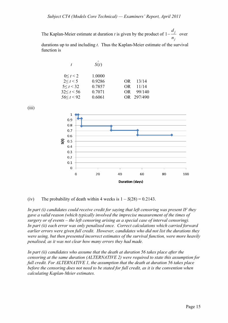
Subject CT4 (Models Core Technical) — Examiners’ Report, April 2011
Page 15
The Kaplan-Meier estimate at duration t is given by the product of 1 j
j
dn
− over
durations up to and including t. Thus the Kaplan-Meier estimate of the survival function is
t ^( )S t 0≤ t < 2 1.0000 2≤ t < 5 0.9286 OR 13/14 5≤ t < 32 0.7857 OR 11/14 32≤ t < 56 0.7071 OR 99/140 56≤ t < 92 0.6061 OR 297/490 (iii)
(iv) The probability of death within 4 weeks is 1 – S(28) = 0.2143.
In part (i) candidates could receive credit for saying that left censoring was present IF they gave a valid reason (which typically involved the imprecise measurement of the times of surgery or of events – the left censoring arising as a special case of interval censoring). In part (ii) each error was only penalised once. Correct calculations which carried forward earlier errors were given full credit. However, candidates who did not list the durations they were using, but then presented incorrect estimates of the survival function, were more heavily penalised, as it was not clear how many errors they had made. In part (ii) candidates who assume that the death at duration 56 takes place after the censoring at the same duration (ALTERNATIVE 2) were required to state this assumption for full credit. For ALTERNATIVE 1, the assumption that the death at duration 56 takes place before the censoring does not need to be stated for full credit, as it is the convention when calculating Kaplan-Meier estimates.
Subject CT4 (Models Core Technical) — Examiners’ Report, April 2011
Page 16
In part (iii) the plotted function should be consistent with the answer to part (ii). If the answer to part (ii) was incorrect but the incorrect answer to part (ii) was correctly plotted in part (iii), full credit could be awarded to part (iii). Question 11 (i) The chi-squared test is a suitable overall test.
Let xμ be the force of mortality in age-group x in the sample. Let s
xμ be the force of mortality in age group x in the national population. Let c
xE be the central exposed to risk in the sample.
Then if c c sx x x x
x c sx x
E EzE
μ − μ=
μ
the test statistic is 2 2
x mx
z χ∑ ∼ ,
THEN EITHER
where m is the number of age groups, which in this case is 8.
The calculations are shown below. Age-group Expected deaths zx 2
xz
5–14 18.7935 –1.3364 1.7860 15–24 50.5460 –0.4988 0.2488 25–34 59.8842 –1.0188 1.0380 35–44 53.3092 –0.4532 0.2054 45–54 39.6396 –1.0546 1.1121 55–64 23.4140 –0.0856 0.0073 65–74 13.3926 –0.1073 0.0115
75–84 1.8200 0.8747 0.7651 Therefore the value of the test statistic is 5.1742.
The critical value of the chi-squared distribution at the 5% level of significance with 8
degrees of freedom is 15.51.
Since 5.1742 < 15.51 we do not reject the null hypothesis that the mortality rate from tuberculosis in the sample is the same as that in the national population.
Subject CT4 (Models Core Technical) — Examiners’ Report, April 2011
Page 17
OR
where m is the number of age groups, which in this case is 7, because we should combine age groups 65–74 and 75–84 as the expected number of deaths in age group 75–84 years is less than 5 The calculations are shown below.
Age-group Expected deaths zx 2
xz
5–14 18.7935 –1.3364 1.7860 15–24 50.5460 –0.4988 0.2488 25–34 59.8842 –1.0188 1.0380 35–44 53.3092 –0.4532 0.2054 45–54 39.6396 –1.0546 1.1121 55–64 23.4140 –0.0856 0.0073 65–84 15.2126 0.2019 0.0408
Therefore the value of the test statistic is 4.438.
The critical value of the chi-squared distribution at the 5% level of significance with 7
degrees of freedom is 14.07.
Since 4.438 < 14.07 we do not reject the null hypothesis that the mortality rate from tuberculosis in the sample is the same as that in the national population
(ii) (a) Small bias which is not great enough for the chi-squared test to detect.
EITHER (b) Signs test
Under the null hypothesis that the mortality rate from tuberculosis in the
sample is the same as that in the national population,
the number of positive signs is distributed Binomial (m, 0.5), where m is the number of ages. We have 1 positive sign. The probability of 1 or fewer positive signs is given by
8 88 80.5 0.5 0.0352
0 1⎛ ⎞ ⎛ ⎞
+ =⎜ ⎟ ⎜ ⎟⎝ ⎠ ⎝ ⎠
.
Subject CT4 (Models Core Technical) — Examiners’ Report, April 2011
Page 18
OR (if only 7 age groups are being used)
7 77 70.5 0.5 0.0625
0 1⎛ ⎞ ⎛ ⎞
+ =⎜ ⎟ ⎜ ⎟⎝ ⎠ ⎝ ⎠
.
We use a two-tailed test (since too few or too many positive signs would be a problem)
so we reject the null hypothesis if the probability of 1 or fewer positive signs is less than 0.025.
Since 0.0352 (or 0.0625) > 0.025 we do not reject the null hypothesis. OR (b) Cumulative deviations test Under the null hypothesis that the mortality rate from tuberculosis in the
sample is the same as that in the national population
the test statistic
( )Normal(0,1)
c c sx x x x
xc sx x
x
E E
E
μ − μ
μ
∑
∑∼
The calculations are shown in the table below
Age-group c c s
x x x xE Eμ − μ c sx xE μ
5–14 –5.7935 18.7935 15–24 –3.5460 50.5460 25–34 –7.8842 59.8842 35–44 –3.3092 53.3092 45–54 –6.6396 39.6396 55–64 –0.4140 23.4140 65–74 –0.3926 13.3926 75–84 1.1800 1.8200
Σ –26.7991 260.7991
So the value of the test statistic is 26.7991 1.6595260.7991−
= .
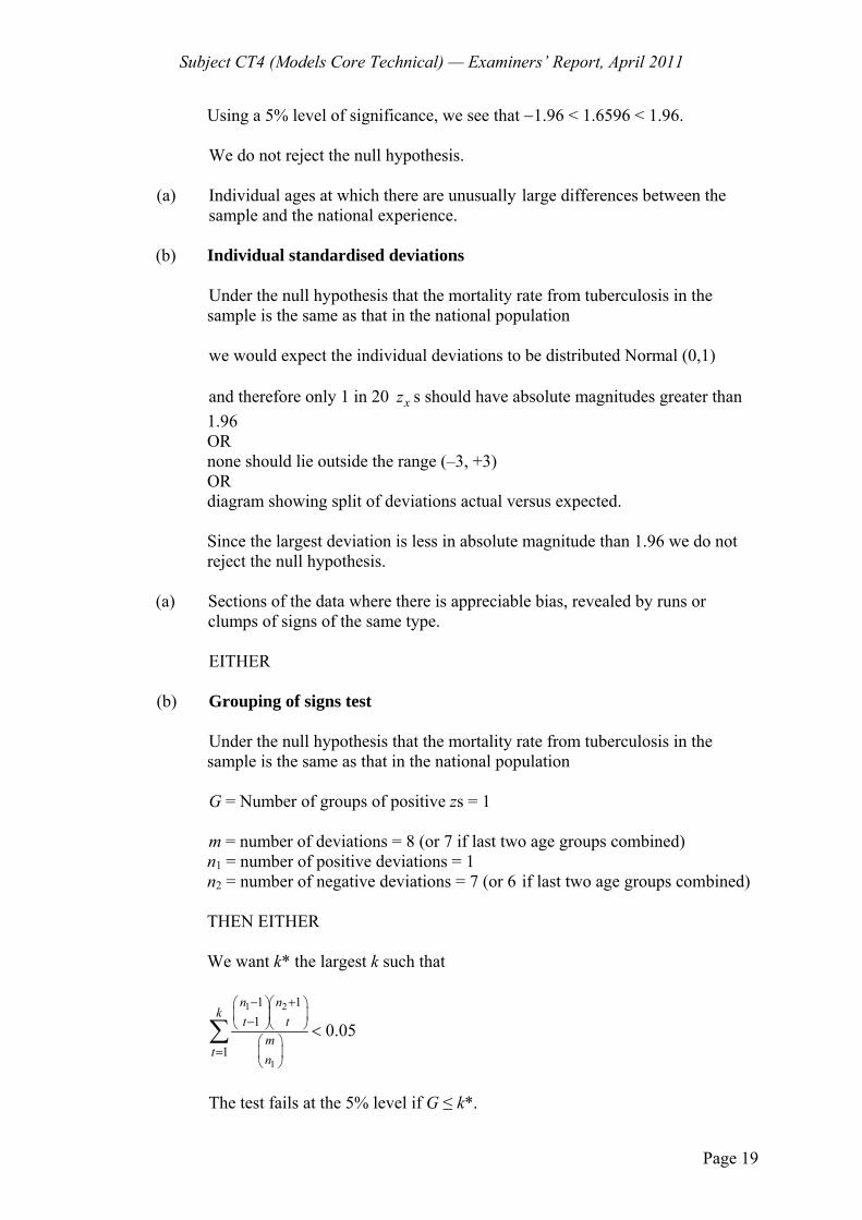
Subject CT4 (Models Core Technical) — Examiners’ Report, April 2011
Page 19
Using a 5% level of significance, we see that −1.96 < 1.6596 < 1.96.
We do not reject the null hypothesis. (a) Individual ages at which there are unusually large differences between the sample and the national experience.
(b) Individual standardised deviations
Under the null hypothesis that the mortality rate from tuberculosis in the sample is the same as that in the national population we would expect the individual deviations to be distributed Normal (0,1) and therefore only 1 in 20 xz s should have absolute magnitudes greater than 1.96 OR none should lie outside the range (–3, +3) OR diagram showing split of deviations actual versus expected.
Since the largest deviation is less in absolute magnitude than 1.96 we do not
reject the null hypothesis.
(a) Sections of the data where there is appreciable bias, revealed by runs or clumps of signs of the same type.
EITHER (b) Grouping of signs test
Under the null hypothesis that the mortality rate from tuberculosis in the sample is the same as that in the national population G = Number of groups of positive zs = 1 m = number of deviations = 8 (or 7 if last two age groups combined) n1 = number of positive deviations = 1 n2 = number of negative deviations = 7 (or 6 if last two age groups combined) THEN EITHER We want k* the largest k such that
1 2
1
1 11
10.05
− +⎛ ⎞⎛ ⎞⎜ ⎟⎜ ⎟−⎝ ⎠⎝ ⎠
⎛ ⎞= ⎜ ⎟
⎝ ⎠
<∑n n
kt t
mt n The test fails at the 5% level if G ≤ k*.
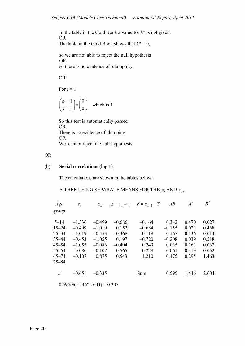
Subject CT4 (Models Core Technical) — Examiners’ Report, April 2011
Page 20
In the table in the Gold Book a value for k* is not given, OR The table in the Gold Book shows that k* = 0, so we are not able to reject the null hypothesis OR so there is no evidence of clumping. OR For t = 1
1 1 01 0
nt−⎛ ⎞ ⎛ ⎞
=⎜ ⎟ ⎜ ⎟−⎝ ⎠ ⎝ ⎠which is 1
So this test is automatically passed
OR There is no evidence of clumping OR We cannot reject the null hypothesis. OR (b) Serial correlations (lag 1) The calculations are shown in the tables below. EITHER USING SEPARATE MEANS FOR THE xz AND 1xz +
Age zx zx xA z z= − 1xB z z+= − AB 2A 2B group
5–14 –1.336 –0.499 –0.686 –0.164 0.342 0.470 0.027 15–24 –0.499 –1.019 0.152 –0.684 –0.155 0.023 0.468 25–34 –1.019 –0.453 –0.368 –0.118 0.167 0.136 0.014 35–44 –0.453 –1.055 0.197 –0.720 –0.208 0.039 0.518 45–54 –1.055 –0.086 –0.404 0.249 0.035 0.163 0.062 55–64 –0.086 –0.107 0.565 0.228 –0.061 0.319 0.052 65–74 –0.107 0.875 0.543 1.210 0.475 0.295 1.463 75–84 z –0.651 –0.335 Sum 0.595 1.446 2.604
0.595/√(1.446*2.604) = 0.307
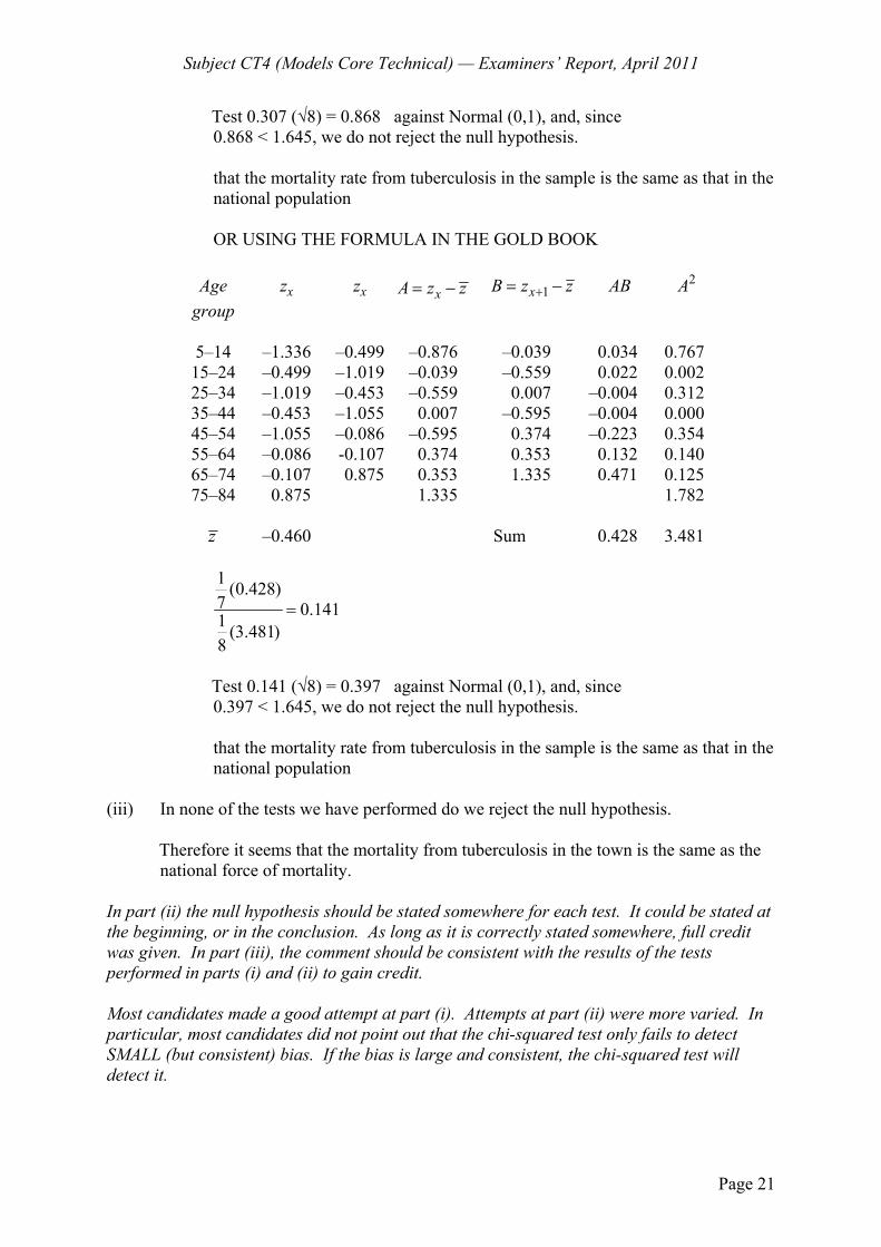
Subject CT4 (Models Core Technical) — Examiners’ Report, April 2011
Page 21
Test 0.307 (√8) = 0.868 against Normal (0,1), and, since 0.868 < 1.645, we do not reject the null hypothesis.
that the mortality rate from tuberculosis in the sample is the same as that in the national population
OR USING THE FORMULA IN THE GOLD BOOK
Age zx zx xA z z= − 1xB z z+= − AB 2A group
5–14 –1.336 –0.499 –0.876 –0.039 0.034 0.767 15–24 –0.499 –1.019 –0.039 –0.559 0.022 0.002 25–34 –1.019 –0.453 –0.559 0.007 –0.004 0.312 35–44 –0.453 –1.055 0.007 –0.595 –0.004 0.000 45–54 –1.055 –0.086 –0.595 0.374 –0.223 0.354 55–64 –0.086 -0.107 0.374 0.353 0.132 0.140 65–74 –0.107 0.875 0.353 1.335 0.471 0.125 75–84 0.875 1.335 1.782 z –0.460 Sum 0.428 3.481
1 (0.428)7 0.1411 (3.481)8
=
Test 0.141 (√8) = 0.397 against Normal (0,1), and, since 0.397 < 1.645, we do not reject the null hypothesis.
that the mortality rate from tuberculosis in the sample is the same as that in the national population
(iii) In none of the tests we have performed do we reject the null hypothesis.
Therefore it seems that the mortality from tuberculosis in the town is the same as the national force of mortality.
In part (ii) the null hypothesis should be stated somewhere for each test. It could be stated at the beginning, or in the conclusion. As long as it is correctly stated somewhere, full credit was given. In part (iii), the comment should be consistent with the results of the tests performed in parts (i) and (ii) to gain credit. Most candidates made a good attempt at part (i). Attempts at part (ii) were more varied. In particular, most candidates did not point out that the chi-squared test only fails to detect SMALL (but consistent) bias. If the bias is large and consistent, the chi-squared test will detect it.
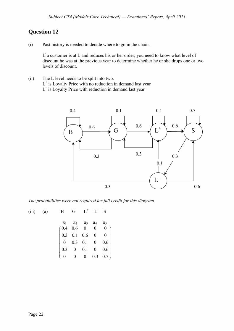
Subject CT4 (Models Core Technical) — Examiners’ Report, April 2011
Page 22
Question 12 (i) Past history is needed to decide where to go in the chain.
If a customer is at L and reduces his or her order, you need to know what level of
discount he was at the previous year to determine whether he or she drops one or two levels of discount.
(ii) The L level needs to be split into two. L+ is Loyalty Price with no reduction in demand last year L– is Loyalty Price with reduction in demand last year
The probabilities were not required for full credit for this diagram. (iii) (a) B G L+ L– S
π1 π2 π3 π4 π5
0.4 0.6 0 0 00.3 0.1 0.6 0 00 0.3 0.1 0 0.6
0.3 0 0.1 0 0.60 0 0 0.3 0.7
⎛ ⎞⎜ ⎟⎜ ⎟⎜ ⎟⎜ ⎟⎜ ⎟⎜ ⎟⎝ ⎠
0.1 0.1 0.7
B G S
L–
0.6 L+
0.6 0.6
0.3 0.6
0.3 0.1
0.4
0.3 0.3
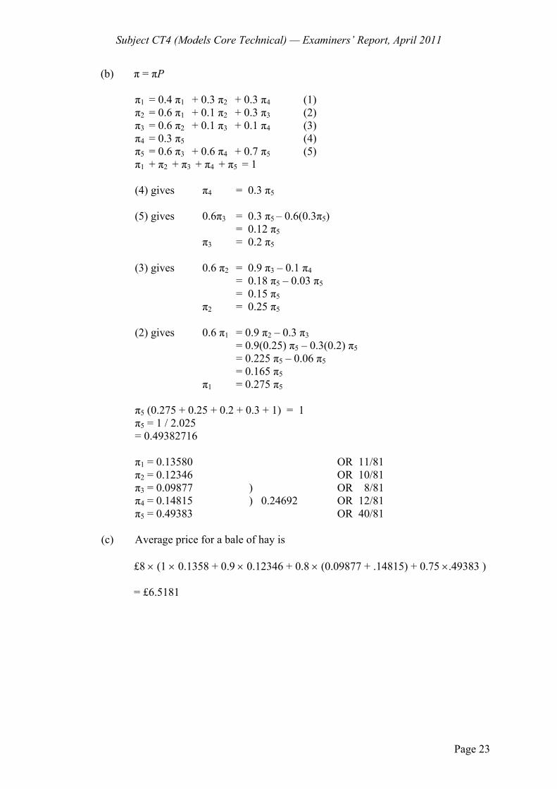
Subject CT4 (Models Core Technical) — Examiners’ Report, April 2011
Page 23
(b) π = πP π1 = 0.4 π1 + 0.3 π2 + 0.3 π4 (1) π2 = 0.6 π1 + 0.1 π2 + 0.3 π3 (2) π3 = 0.6 π2 + 0.1 π3 + 0.1 π4 (3) π4 = 0.3 π5 (4) π5 = 0.6 π3 + 0.6 π4 + 0.7 π5 (5) π1 + π2 + π3 + π4 + π5 = 1 (4) gives π4 = 0.3 π5 (5) gives 0.6π3 = 0.3 π5 – 0.6(0.3π5) = 0.12 π5 π3 = 0.2 π5 (3) gives 0.6 π2 = 0.9 π3 – 0.1 π4 = 0.18 π5 – 0.03 π5 = 0.15 π5 π2 = 0.25 π5 (2) gives 0.6 π1 = 0.9 π2 – 0.3 π3 = 0.9(0.25) π5 – 0.3(0.2) π5 = 0.225 π5 – 0.06 π5 = 0.165 π5 π1 = 0.275 π5 π5 (0.275 + 0.25 + 0.2 + 0.3 + 1) = 1 π5 = 1 / 2.025 = 0.49382716 π1 = 0.13580 OR 11/81 π2 = 0.12346 OR 10/81 π3 = 0.09877 ) OR 8/81 π4 = 0.14815 ) 0.24692 OR 12/81 π5 = 0.49383 OR 40/81
(c) Average price for a bale of hay is
£8 × (1 × 0.1358 + 0.9 × 0.12346 + 0.8 × (0.09877 + .14815) + 0.75 ×.49383 ) = £6.5181
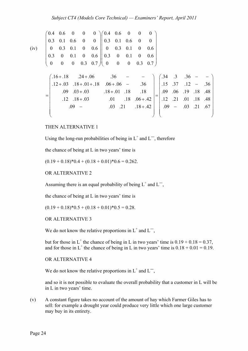
Subject CT4 (Models Core Technical) — Examiners’ Report, April 2011
Page 24
(iv)
0.4 0.6 0 0 00.3 0.1 0.6 0 00 0.3 0.1 0 0.6
0.3 0 0.1 0 0.60 0 0 0.3 0.7
⎛ ⎞⎜ ⎟⎜ ⎟⎜ ⎟⎜ ⎟⎜ ⎟⎜ ⎟⎝ ⎠
0.4 0.6 0 0 00.3 0.1 0.6 0 00 0.3 0.1 0 0.6
0.3 0 0.1 0 0.60 0 0 0.3 0.7
⎛ ⎞⎜ ⎟⎜ ⎟⎜ ⎟⎜ ⎟⎜ ⎟⎜ ⎟⎝ ⎠
.16 .18 .24 .06 .36
.12 .03 .18 .01 .18 .06 .06 .36.09 .03 .03 .18 .01 .18 .18.12 .18 .03 .01 .18 .06 .42
.09 .03 .21 .18 .42
+ + − −⎛ ⎞⎜ ⎟+ + + + −⎜ ⎟⎜ ⎟+ +
= ⎜ ⎟+ +⎜ ⎟
⎜ ⎟− +⎜ ⎟⎜ ⎟⎝ ⎠
.34 .3 .36
.15 .37 .12 .36
.09 .06 .19 .18 .48
.12 .21 .01 .18 .48.09 .03 .21 .67
− −⎛ ⎞⎜ ⎟−⎜ ⎟⎜ ⎟
= ⎜ ⎟⎜ ⎟⎜ ⎟−⎜ ⎟⎜ ⎟⎝ ⎠
THEN ALTERNATIVE 1 Using the long-run probabilities of being in L+ and L―, therefore the chance of being at L in two years’ time is (0.19 + 0.18)*0.4 + (0.18 + 0.01)*0.6 = 0.262. OR ALTERNATIVE 2 Assuming there is an equal probability of being L+ and L―, the chance of being at L in two years’ time is (0.19 + 0.18)*0.5 + (0.18 + 0.01)*0.5 = 0.28. OR ALTERNATIVE 3 We do not know the relative proportions in L+ and L―, but for those in L+ the chance of being in L in two years’ time is 0.19 + 0.18 = 0.37, and for those in L+ the chance of being in L in two years’ time is 0.18 + 0.01 = 0.19. OR ALTERNATIVE 4 We do not know the relative proportions in L+ and L―, and so it is not possible to evaluate the overall probability that a customer in L will be in L in two years’ time.
(v) A constant figure takes no account of the amount of hay which Farmer Giles has to sell: for example a drought year could produce very little which one large customer may buy in its entirety.

Subject CT4 (Models Core Technical) — Examiners’ Report, April 2011
Page 25
The amount of hay in the local market is important.
Another supplier may try a heavy discounted year to get into the market.
Customers’ behaviour may depend on the discount level they are at.
There may be national trends in the demand for hay e.g. a sudden trend towards vegetarianism.
A 60% chance of increasing may be implausible, as field space is likely to be limited,
so a constant increase in numbers unlikely. Customers’ behaviour may depend on the amount of hay they typically purchase. A common error in part (ii) was to split state G into two states as well as splitting state L. This is not required to model the system with the Markov property and so was penalised. However, candidates who split state G and then followed through with a correct matrix in part (iii)(a) and correct solutions in part (iii)(b) were not penalised again. Note that splitting state G should produce the same answer to part (iii)(b), though more work will be needed! In part (iv) candidates who adopted ALTERNATIVE 4, in which they declined to give an overall answer on the grounds that they do not know the proprotions in states L+ and L― , were only given credit if they presented a reasoned argument with evidence. In part (v) credit was given for other sensible suggestions.
END OF EXAMINERS’ REPORT

INSTITUTE AND FACULTY OF ACTUARIES
EXAMINATION
7 October 2011 (am)
Subject CT4 — Models Core Technical
Time allowed: Three hours
INSTRUCTIONS TO THE CANDIDATE
1. Enter all the candidate and examination details as requested on the front of your answer booklet.
2. You must not start writing your answers in the booklet until instructed to do so by the
supervisor. 3. Mark allocations are shown in brackets. 4. Attempt all 11 questions, beginning your answer to each question on a separate sheet. 5. Candidates should show calculations where this is appropriate.
Graph paper is NOT required for this paper.
AT THE END OF THE EXAMINATION
Hand in BOTH your answer booklet, with any additional sheets firmly attached, and this question paper.
In addition to this paper you should have available the 2002 edition of the Formulae and Tables and your own electronic calculator from the approved list.
CT4 S2011 © Institute and Faculty of Actuaries
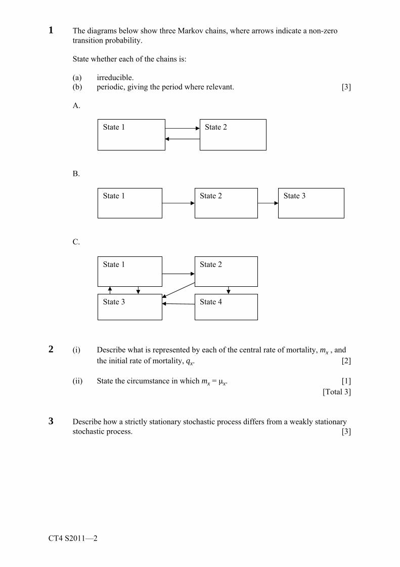
CT4 S2011—2
1 The diagrams below show three Markov chains, where arrows indicate a non-zero transition probability.
State whether each of the chains is: (a) irreducible. (b) periodic, giving the period where relevant. [3] A.
B.
C.
2 (i) Describe what is represented by each of the central rate of mortality, mx , and
the initial rate of mortality, qx. [2] (ii) State the circumstance in which mx = μx. [1] [Total 3]
3 Describe how a strictly stationary stochastic process differs from a weakly stationary stochastic process. [3]
State 1 State 2
State 1 State 2
State 3 State 4
State 1 State 2 State 3
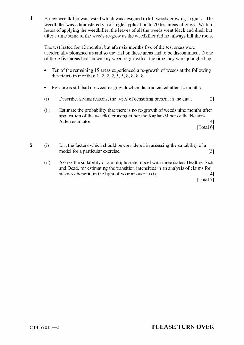
CT4 S2011—3 PLEASE TURN OVER
4 A new weedkiller was tested which was designed to kill weeds growing in grass. The weedkiller was administered via a single application to 20 test areas of grass. Within hours of applying the weedkiller, the leaves of all the weeds went black and died, but after a time some of the weeds re-grew as the weedkiller did not always kill the roots.
The test lasted for 12 months, but after six months five of the test areas were
accidentally ploughed up and so the trial on these areas had to be discontinued. None of these five areas had shown any weed re-growth at the time they were ploughed up.
• Ten of the remaining 15 areas experienced a re-growth of weeds at the following
durations (in months): 1, 2, 2, 2, 5, 5, 8, 8, 8, 8. • Five areas still had no weed re-growth when the trial ended after 12 months.
(i) Describe, giving reasons, the types of censoring present in the data. [2] (ii) Estimate the probability that there is no re-growth of weeds nine months after
application of the weedkiller using either the Kaplan-Meier or the Nelson-Aalen estimator. [4]
[Total 6] 5 (i) List the factors which should be considered in assessing the suitability of a
model for a particular exercise. [3] (ii) Assess the suitability of a multiple state model with three states: Healthy, Sick
and Dead, for estimating the transition intensities in an analysis of claims for sickness benefit, in the light of your answer to (i). [4]
[Total 7]
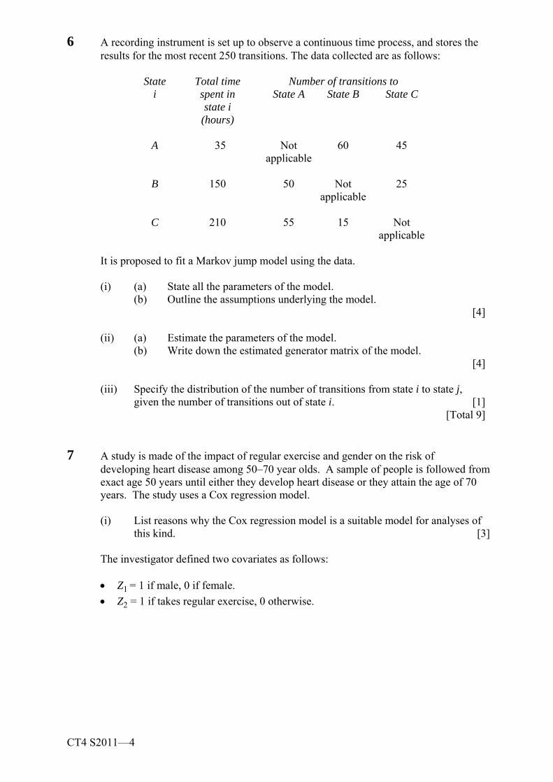
CT4 S2011—4
6 A recording instrument is set up to observe a continuous time process, and stores the results for the most recent 250 transitions. The data collected are as follows:
State Total time Number of transitions to
i spent in State A State B State C state i (hours)
A 35 Not 60 45 applicable B 150 50 Not 25 applicable C 210 55 15 Not
applicable It is proposed to fit a Markov jump model using the data. (i) (a) State all the parameters of the model. (b) Outline the assumptions underlying the model.
[4] (ii) (a) Estimate the parameters of the model. (b) Write down the estimated generator matrix of the model.
[4]
(iii) Specify the distribution of the number of transitions from state i to state j, given the number of transitions out of state i. [1]
[Total 9]
7 A study is made of the impact of regular exercise and gender on the risk of
developing heart disease among 50–70 year olds. A sample of people is followed from exact age 50 years until either they develop heart disease or they attain the age of 70 years. The study uses a Cox regression model.
(i) List reasons why the Cox regression model is a suitable model for analyses of
this kind. [3]
The investigator defined two covariates as follows:
• Z1 = 1 if male, 0 if female. • Z2 = 1 if takes regular exercise, 0 otherwise.
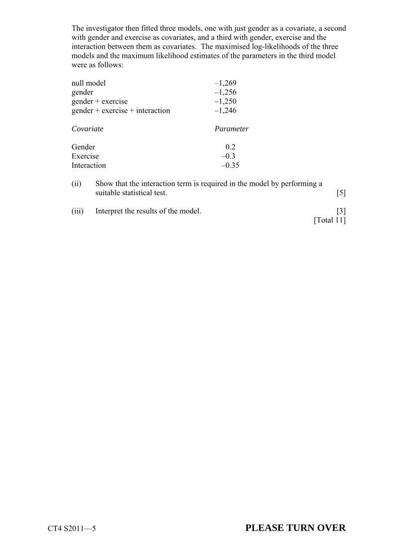
CT4 S2011—5 PLEASE TURN OVER
The investigator then fitted three models, one with just gender as a covariate, a second with gender and exercise as covariates, and a third with gender, exercise and the interaction between them as covariates. The maximised log-likelihoods of the three models and the maximum likelihood estimates of the parameters in the third model were as follows:
null model –1,269 gender –1,256 gender + exercise –1,250 gender + exercise + interaction –1,246 Covariate Parameter Gender 0.2 Exercise –0.3 Interaction –0.35 (ii) Show that the interaction term is required in the model by performing a
suitable statistical test. [5] (iii) Interpret the results of the model. [3] [Total 11]
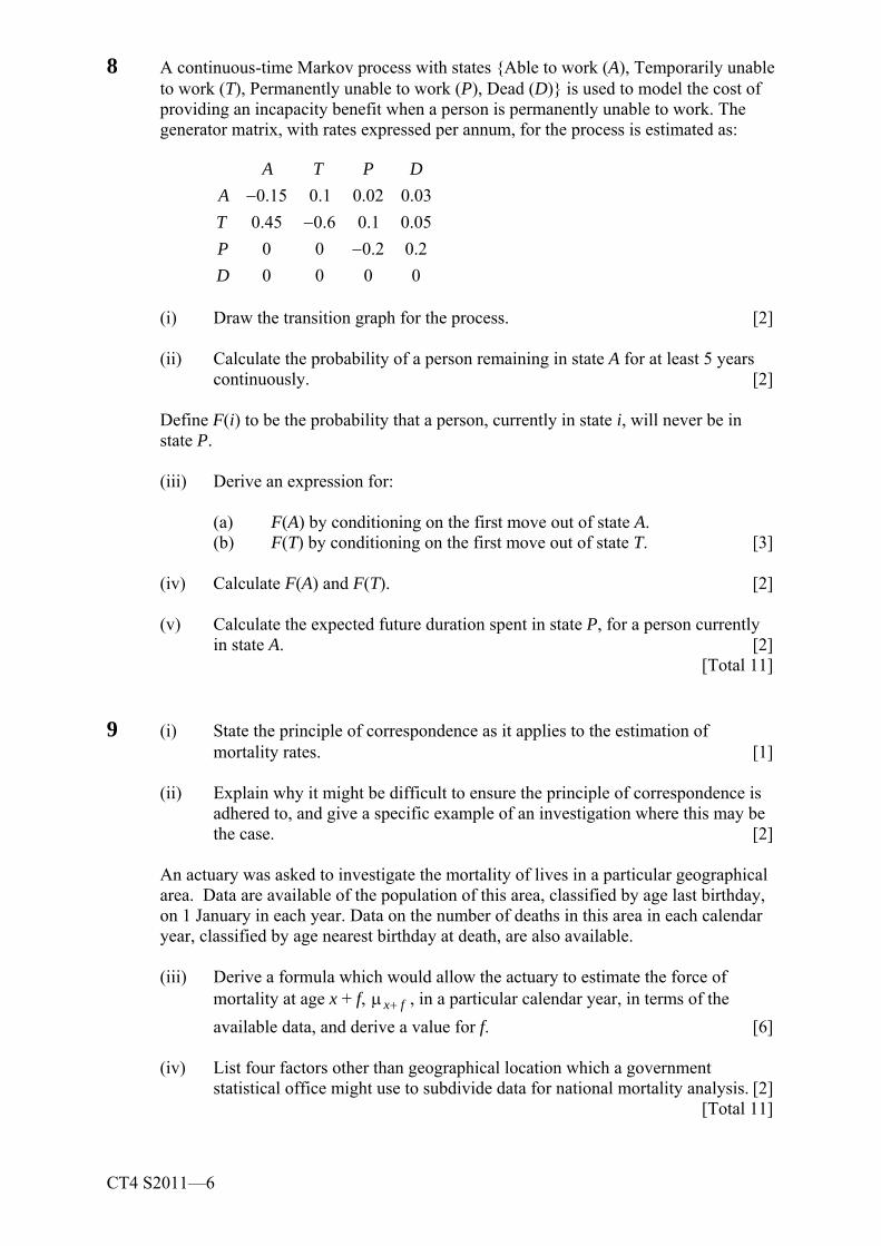
CT4 S2011—6
8 A continuous-time Markov process with states {Able to work (A), Temporarily unable to work (T), Permanently unable to work (P), Dead (D)} is used to model the cost of providing an incapacity benefit when a person is permanently unable to work. The generator matrix, with rates expressed per annum, for the process is estimated as:
0.15 0.1 0.02 0.030.45 0.6 0.1 0.05
0 0 0.2 0.20 0 0 0
A T P DATPD
−−
−
(i) Draw the transition graph for the process. [2] (ii) Calculate the probability of a person remaining in state A for at least 5 years
continuously. [2] Define F(i) to be the probability that a person, currently in state i, will never be in
state P. (iii) Derive an expression for:
(a) F(A) by conditioning on the first move out of state A. (b) F(T) by conditioning on the first move out of state T. [3] (iv) Calculate F(A) and F(T). [2] (v) Calculate the expected future duration spent in state P, for a person currently
in state A. [2] [Total 11] 9 (i) State the principle of correspondence as it applies to the estimation of
mortality rates. [1] (ii) Explain why it might be difficult to ensure the principle of correspondence is
adhered to, and give a specific example of an investigation where this may be the case. [2]
An actuary was asked to investigate the mortality of lives in a particular geographical area. Data are available of the population of this area, classified by age last birthday, on 1 January in each year. Data on the number of deaths in this area in each calendar year, classified by age nearest birthday at death, are also available.
(iii) Derive a formula which would allow the actuary to estimate the force of mortality at age x + f, x f+μ , in a particular calendar year, in terms of the available data, and derive a value for f. [6]
(iv) List four factors other than geographical location which a government
statistical office might use to subdivide data for national mortality analysis. [2] [Total 11]
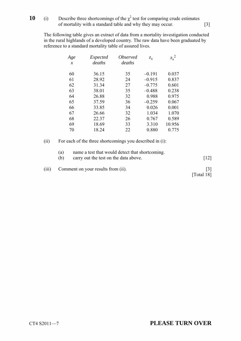
CT4 S2011—7 PLEASE TURN OVER
10 (i) Describe three shortcomings of the χ2 test for comparing crude estimates of mortality with a standard table and why they may occur. [3]
The following table gives an extract of data from a mortality investigation conducted in the rural highlands of a developed country. The raw data have been graduated by reference to a standard mortality table of assured lives.
Age x
Expected deaths
Observed deaths
zx
zx
2
60 61 62 63 64 65 66 67 68 69 70
36.15 28.92 31.34 38.01 26.88 37.59 33.85 26.66 22.37 18.69 18.24
35 24 27 35 32 36 34 32 26 33 22
–0.191 –0.915 –0.775 –0.488
0.988 –0.259
0.026 1.034 0.767 3.310 0.880
0.037 0.837 0.601 0.238 0.975 0.067 0.001 1.070 0.589
10.956 0.775
(ii) For each of the three shortcomings you described in (i): (a) name a test that would detect that shortcoming. (b) carry out the test on the data above. [12] (iii) Comment on your results from (ii). [3] [Total 18]
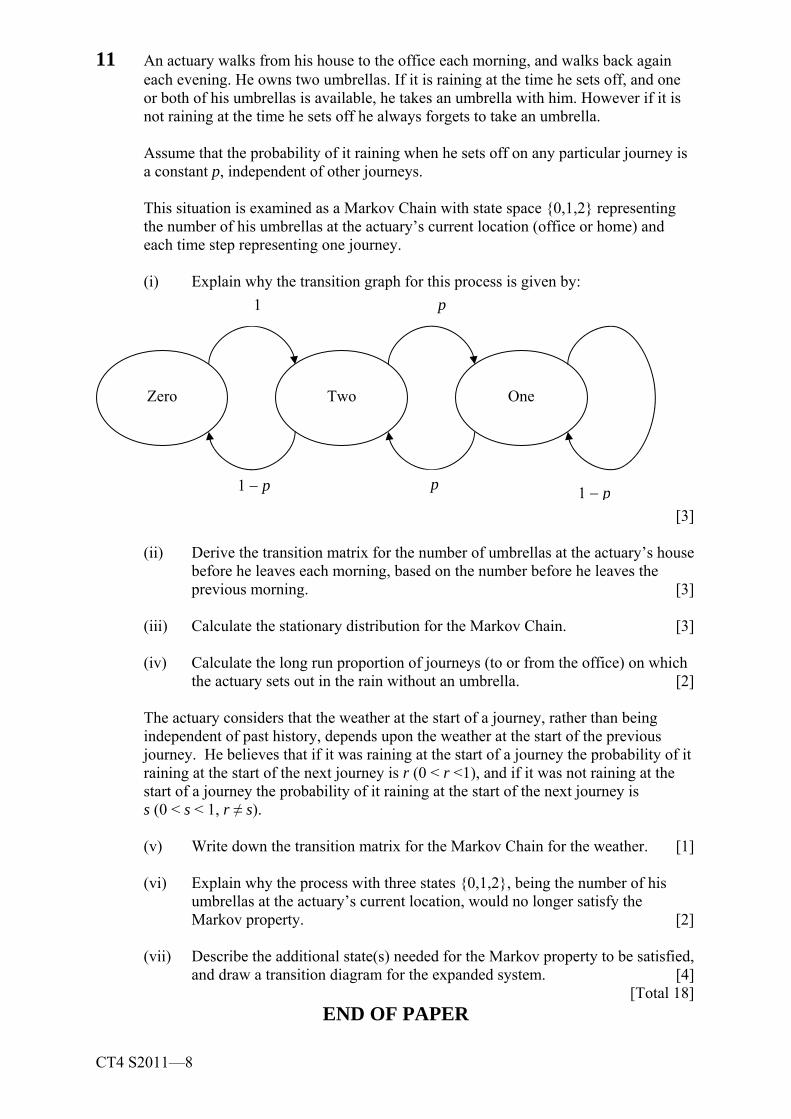
CT4 S2011—8
11 An actuary walks from his house to the office each morning, and walks back again each evening. He owns two umbrellas. If it is raining at the time he sets off, and one or both of his umbrellas is available, he takes an umbrella with him. However if it is not raining at the time he sets off he always forgets to take an umbrella.
Assume that the probability of it raining when he sets off on any particular journey is
a constant p, independent of other journeys. This situation is examined as a Markov Chain with state space {0,1,2} representing
the number of his umbrellas at the actuary’s current location (office or home) and each time step representing one journey.
(i) Explain why the transition graph for this process is given by:
[3] (ii) Derive the transition matrix for the number of umbrellas at the actuary’s house
before he leaves each morning, based on the number before he leaves the previous morning. [3]
(iii) Calculate the stationary distribution for the Markov Chain. [3] (iv) Calculate the long run proportion of journeys (to or from the office) on which
the actuary sets out in the rain without an umbrella. [2] The actuary considers that the weather at the start of a journey, rather than being independent of past history, depends upon the weather at the start of the previous journey. He believes that if it was raining at the start of a journey the probability of it raining at the start of the next journey is r (0 < r <1), and if it was not raining at the start of a journey the probability of it raining at the start of the next journey is s (0 < s < 1, r ≠ s).
(v) Write down the transition matrix for the Markov Chain for the weather. [1] (vi) Explain why the process with three states {0,1,2}, being the number of his
umbrellas at the actuary’s current location, would no longer satisfy the Markov property. [2]
(vii) Describe the additional state(s) needed for the Markov property to be satisfied,
and draw a transition diagram for the expanded system. [4] [Total 18]
END OF PAPER
1 − p
p
One
Two
Zero
1
p 1 − p

INSTITUTE AND FACULTY OF ACTUARIES
EXAMINERS’ REPORT
September 2011 examinations
Subject CT4 — Models Core Technical
Purpose of Examiners’ Reports The Examiners’ Report is written by the Principal Examiner with the aim of helping candidates, both those who are sitting the examination for the first time and who are using past papers as a revision aid, and also those who have previously failed the subject. The Examiners are charged by Council with examining the published syllabus. Although Examiners have access to the Core Reading, which is designed to interpret the syllabus, the Examiners are not required to examine the content of Core Reading. Notwithstanding that, the questions set, and the following comments, will generally be based on Core Reading. For numerical questions the Examiners’ preferred approach to the solution is reproduced in this report. Other valid approaches are always given appropriate credit; where there is a commonly used alternative approach, this is also noted in the report. For essay-style questions, and particularly the open-ended questions in the later subjects, this report contains all the points for which the Examiners awarded marks. This is much more than a model solution – it would be impossible to write down all the points in the report in the time allowed for the question. T J Birse Chairman of the Board of Examiners December 2011
© Institute and Faculty of Actuaries

Subject CT4 (Models Core Technical) — Examiners’ Report, September 2011
Page 2
General comments on Subject CT4 Subject CT4 comprises five main sections: (1) a study of the properties of models in general, and their uses for actuaries, including advantages and disadvantages (and a comparison of alternative models of the same processes); (2) stochastic processes, especially Markov chains and Markov jump processes; (3) models of a random variable measuring future lifetime; (4) the calculation of exposed to risk and the application of the principle of correspondence; (5) the reasons why mortality (or other decremental) rates are graduated, and a range of statistical tests used both to compare a set of rates with a previous experience and to test the adherence of a graduated set of rates to the original data. Throughout the subject the emphasis is on estimation and the practical application of models. Theory is kept to the minimum required in order usefully to apply the models to real problems. Different numerical answers may be obtained to those shown in these solutions depending on whether figures obtained from tables or from calculators are used in the calculations but candidates are not penalised for this. However, candidates may be penalised where excessive rounding has been used or where insufficient working is shown. Comments on the September 2011 paper The general performance was slightly worse than in April 2011 but well-prepared candidates scored well across the whole paper. As in previous diets, questions that required an element of explanation or analysis, such as Q5(ii) and Q7(iii) were less well answered than those that just involved calculation. The comments that follow the questions concentrate on areas where candidates could have improved their performance. Candidates approaching the subject for the first time are advised to concentrate their revision in these areas.
Subject CT4 (Models Core Technical) — Examiners’ Report, September 2011
Page 3
Question 1 (a) A Yes, irreducible. B No, not irreducible. C Yes, irreducible. (b) A Yes, period is 2 B No, not periodic. C No, not periodic. This question was well answered, although many candidates failed to identify that C was aperiodic. Question 2 (i) mx is the probability that a life alive between exact ages x and x dies OR mx is the probability of dying between exact ages x and x per person-year lived between exact ages x and x qx is the probability that a life alive at exact age x dies before exact age x [2] (ii) mx and µx are equal when the force of mortality µx+t is constant for 0 ≤ t < 1. Answers to this question were disappointing. In part (i) some candidates defined mx as
1
0
x
t x
q
p dt∫For full credit, candidates who did this were required to explain what this
expression means (e.g. by stating that t xp is the expected amount of time spent alive between x and x+1 by a life alive at age x). Question 3 A stochastic process is said to be strictly stationary if the joint distributions of
1 2, ,...,
nt t tX X X and 1 2, ,...,
nt t t t t tX X X+ + + are identical for all 1 2, , ,..., nt t t t in the time set J and for all integers n. This means that the statistical properties of the process remain unchanged as time elapses. Weak stationarity requires that the mean of the process, ( ) ( )tm t E X= , is constant, and
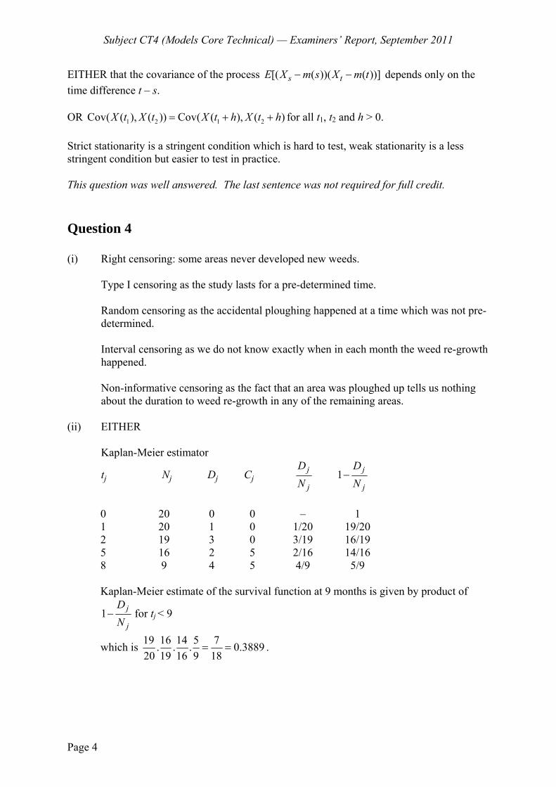
Subject CT4 (Models Core Technical) — Examiners’ Report, September 2011
Page 4
EITHER that the covariance of the process [( ( ))( ( ))]s tE X m s X m t− − depends only on the time difference t – s.
OR 1 2 1 2Cov( ( ), ( )) Cov( ( ), ( )X t X t X t h X t h= + + for all t1, t2 and h > 0.
Strict stationarity is a stringent condition which is hard to test, weak stationarity is a less stringent condition but easier to test in practice. This question was well answered. The last sentence was not required for full credit.
Question 4 (i) Right censoring: some areas never developed new weeds. Type I censoring as the study lasts for a pre-determined time. Random censoring as the accidental ploughing happened at a time which was not pre-
determined. Interval censoring as we do not know exactly when in each month the weed re-growth
happened. Non-informative censoring as the fact that an area was ploughed up tells us nothing
about the duration to weed re-growth in any of the remaining areas. (ii) EITHER Kaplan-Meier estimator
tj Nj Dj Cj j
j
DN
1 j
j
DN
−
0 20 0 0 – 1 1 20 1 0 1/20 19/20 2 19 3 0 3/19 16/19 5 16 2 5 2/16 14/16 8 9 4 5 4/9 5/9
Kaplan-Meier estimate of the survival function at 9 months is given by product of
1 j
j
DN
− for tj < 9
which is 19 16 14 5 7. . . 0.388920 19 16 9 18
= = .
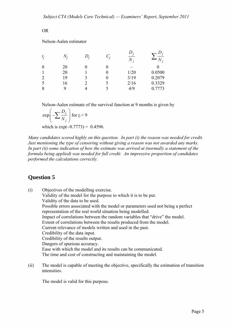
Subject CT4 (Models Core Technical) — Examiners’ Report, September 2011
Page 5
OR Nelson-Aalen estimator
tj Nj Dj Cj j
j
DN
j
j
DN∑
0 20 0 0 – 0 1 20 1 0 1/20 0.0500 2 19 3 0 3/19 0.2079 5 16 2 5 2/16 0.3329 8 9 4 5 4/9 0.7773
Nelson-Aalen estimate of the survival function at 9 months is given by
exp j
j
DN
⎛ ⎞−⎜ ⎟⎜ ⎟⎝ ⎠∑ for tj < 9
which is exp(−0.7773) = 0.4596.
Many candidates scored highly on this question. In part (i) the reason was needed for credit. Just mentioning the type of censoring without giving a reason was not awarded any marks. In part (ii) some indication of how the estimate was arrived at (normally a statement of the formula being applied) was needed for full credit. An impressive proportion of candidates performed the calculations correctly. Question 5 (i) Objectives of the modelling exercise. Validity of the model for the purpose to which it is to be put. Validity of the data to be used. Possible errors associated with the model or parameters used not being a perfect representation of the real world situation being modelled. Impact of correlations between the random variables that “drive” the model. Extent of correlations between the results produced from the model. Current relevance of models written and used in the past. Credibility of the data input. Credibility of the results output. Dangers of spurious accuracy. Ease with which the model and its results can be communicated. The time and cost of constructing and maintaining the model. (ii) The model is capable of meeting the objective, specifically the estimation of transition
intensities. The model is valid for this purpose.
Subject CT4 (Models Core Technical) — Examiners’ Report, September 2011
Page 6
The data required are the total waiting times in each of the states Healthy and Sick for the lives in the investigation during the period of the investigation, together with the number of transitions from Healthy to Sick, from Sick to Healthy, from Healthy to Dead and from Sick to Dead.
Provided these data are available, the data will be valid for the application of the
model.
The model is as good a representation of the real world process as we can obtain.
The model requires that we estimate constant intensities. The results will be credible provided we estimate the intensities separately for short age intervals, over which the assumption of constant transition intensities is credible.
The concept of transition intensities is not intuitively easy for non-specialists to
understand.
The results can be made easier to understand and the results clearer by converting the transition intensities to probabilities – e.g. the probability that a Healthy life aged x will make a sickness claim before he or she is aged x+t years.
Some candidates scored well on part (i), which was standard bookwork, but a disappointing number did not. Answers to part (ii) were variable. To score highly, the points made in part (ii) should relate to those made in part (i). Within this general criterion, sensible points other than those listed above were given credit. Full marks could be obtained for less than is given in the model solution above. Question 6 (i) (a) EITHER The parameters are the rate of leaving state i, λi, for each i, and the jump-chain transition probabilities, rij, for j ≠ i, where rij is the conditional probability that the next transition is to state j given the current state is i.
OR
If the rate of leaving state i, is λi, and rij is the conditional probability that the next transition is to state j given the current state is i. The parameters are μij, where, for i = j, μii = -λi and, for i ≠ j, μij = λi rij.
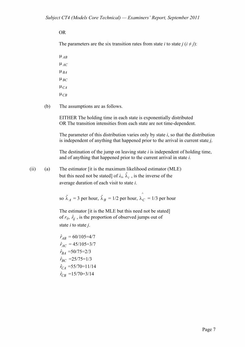
Subject CT4 (Models Core Technical) — Examiners’ Report, September 2011
Page 7
OR The parameters are the six transition rates from state i to state j (i ≠ j):
AB
AC
BA
BC
CA
CB
μμ
μμ
μ
μ
(b) The assumptions are as follows.
EITHER The holding time in each state is exponentially distributed OR The transition intensities from each state are not time-dependent. The parameter of this distribution varies only by state i, so that the distribution is independent of anything that happened prior to the arrival in current state i. The destination of the jump on leaving state i is independent of holding time, and of anything that happened prior to the current arrival in state i. (ii) (a) The estimator [it is the maximum likelihood estimator (MLE) but this need not be stated] of λi, ˆ
iλ , is the inverse of the average duration of each visit to state i.
so ˆAλ = 3 per hour, ˆ
Bλ = 1/2 per hour, ^Cλ = 1/3 per hour
The estimator [it is the MLE but this need not be stated] of rij, ijr , is the proportion of observed jumps out of state i to state j. ABr = 60/105=4/7 ACr = 45/105=3/7 BAr =50/75=2/3 BCr =25/75=1/3 CAr =55/70=11/14 CBr =15/70=3/14
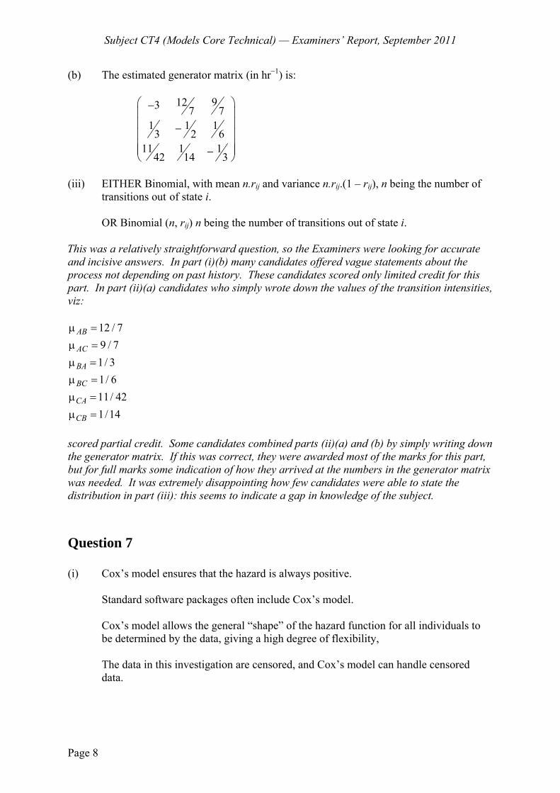
Subject CT4 (Models Core Technical) — Examiners’ Report, September 2011
Page 8
(b) The estimated generator matrix (in hr−1) is:
9123 7 71 1 1
3 2 611 1 1
42 14 3
⎛ ⎞−⎜ ⎟⎜ ⎟−⎜ ⎟⎜ ⎟⎜ ⎟−⎝ ⎠
(iii) EITHER Binomial, with mean n.rij and variance n.rij.(1 – rij), n being the number of transitions out of state i. OR Binomial (n, rij) n being the number of transitions out of state i. This was a relatively straightforward question, so the Examiners were looking for accurate and incisive answers. In part (i)(b) many candidates offered vague statements about the process not depending on past history. These candidates scored only limited credit for this part. In part (ii)(a) candidates who simply wrote down the values of the transition intensities, viz:
12 / 79 / 71/ 31/ 611/ 421/14
AB
AC
BA
BC
CA
CB
μ =μ =
μ =μ =
μ =
μ =
scored partial credit. Some candidates combined parts (ii)(a) and (b) by simply writing down the generator matrix. If this was correct, they were awarded most of the marks for this part, but for full marks some indication of how they arrived at the numbers in the generator matrix was needed. It was extremely disappointing how few candidates were able to state the distribution in part (iii): this seems to indicate a gap in knowledge of the subject. Question 7 (i) Cox’s model ensures that the hazard is always positive. Standard software packages often include Cox’s model. Cox’s model allows the general “shape” of the hazard function for all individuals to be determined by the data, giving a high degree of flexibility, The data in this investigation are censored, and Cox’s model can handle censored data.
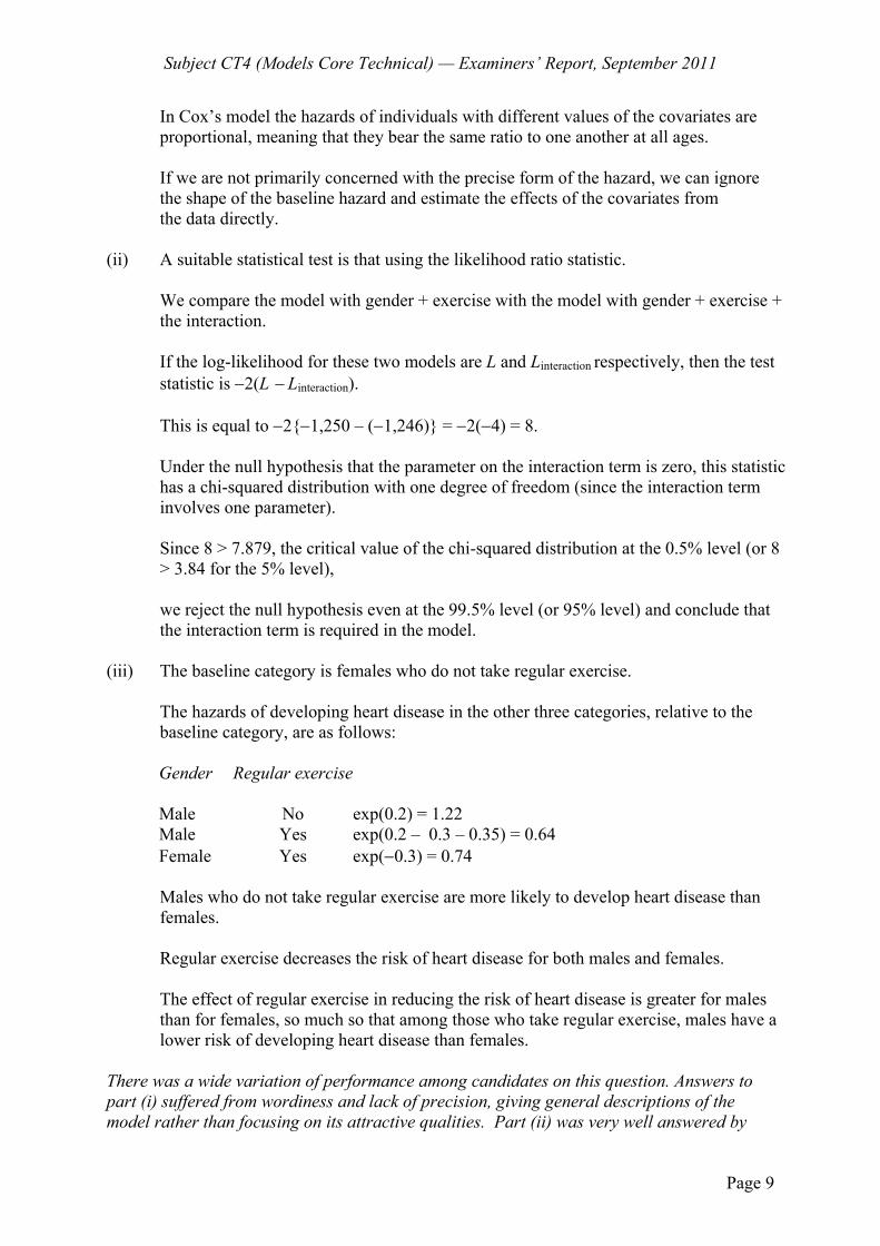
Subject CT4 (Models Core Technical) — Examiners’ Report, September 2011
Page 9
In Cox’s model the hazards of individuals with different values of the covariates are proportional, meaning that they bear the same ratio to one another at all ages. If we are not primarily concerned with the precise form of the hazard, we can ignore the shape of the baseline hazard and estimate the effects of the covariates from the data directly. (ii) A suitable statistical test is that using the likelihood ratio statistic. We compare the model with gender + exercise with the model with gender + exercise + the interaction. If the log-likelihood for these two models are L and Linteraction respectively, then the test statistic is −2(L − Linteraction). This is equal to −2{−1,250 – (−1,246)} = −2(−4) = 8. Under the null hypothesis that the parameter on the interaction term is zero, this statistic has a chi-squared distribution with one degree of freedom (since the interaction term involves one parameter). Since 8 > 7.879, the critical value of the chi-squared distribution at the 0.5% level (or 8 > 3.84 for the 5% level), we reject the null hypothesis even at the 99.5% level (or 95% level) and conclude that the interaction term is required in the model. (iii) The baseline category is females who do not take regular exercise. The hazards of developing heart disease in the other three categories, relative to the baseline category, are as follows:
Gender Regular exercise Male No exp(0.2) = 1.22 Male Yes exp(0.2 – 0.3 – 0.35) = 0.64 Female Yes exp(−0.3) = 0.74
Males who do not take regular exercise are more likely to develop heart disease than females. Regular exercise decreases the risk of heart disease for both males and females. The effect of regular exercise in reducing the risk of heart disease is greater for males than for females, so much so that among those who take regular exercise, males have a lower risk of developing heart disease than females. There was a wide variation of performance among candidates on this question. Answers to part (i) suffered from wordiness and lack of precision, giving general descriptions of the model rather than focusing on its attractive qualities. Part (ii) was very well answered by
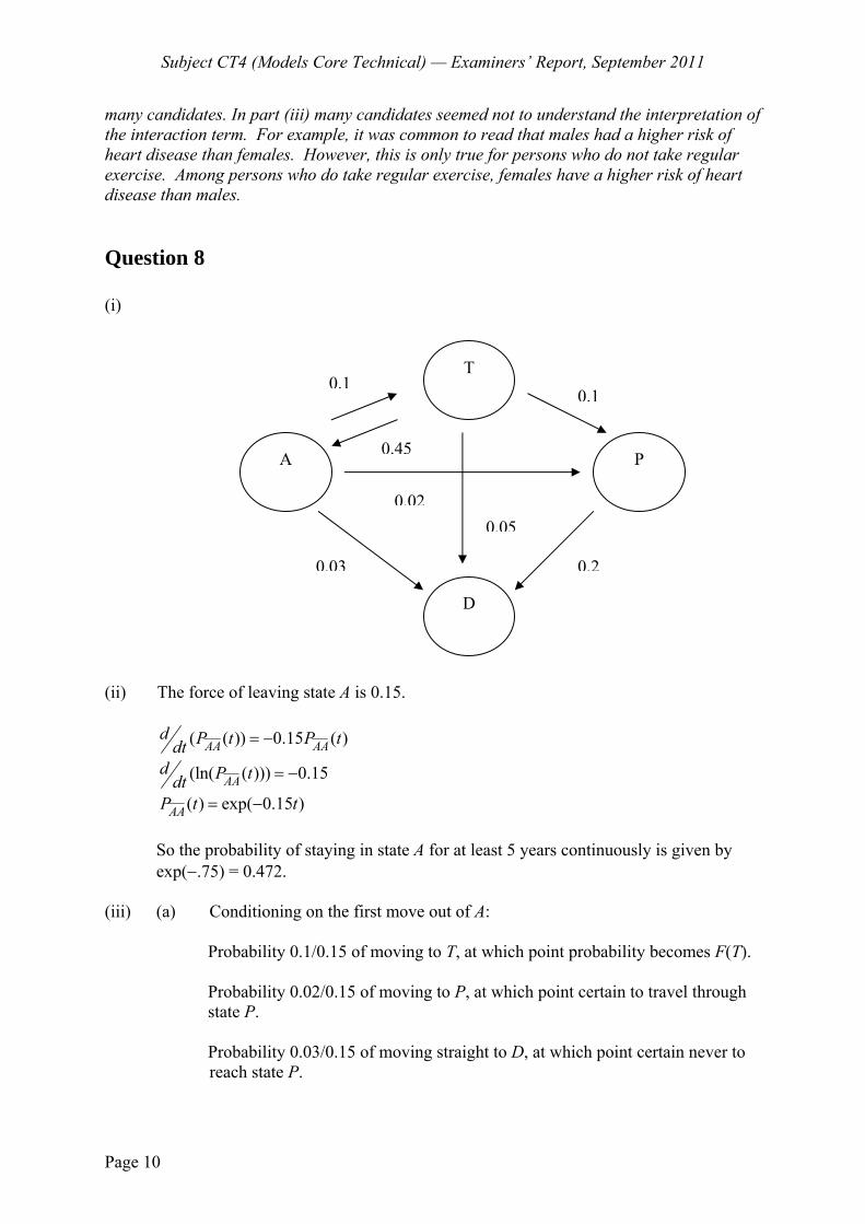
Subject CT4 (Models Core Technical) — Examiners’ Report, September 2011
Page 10
many candidates. In part (iii) many candidates seemed not to understand the interpretation of the interaction term. For example, it was common to read that males had a higher risk of heart disease than females. However, this is only true for persons who do not take regular exercise. Among persons who do take regular exercise, females have a higher risk of heart disease than males. Question 8 (i)
(ii) The force of leaving state A is 0.15. ( ( )) 0.15 ( )AA AA
d P t P tdt = −
(ln( ( ))) 0.15AAd P tdt = −
( ) exp( 0.15 )AAP t t= − So the probability of staying in state A for at least 5 years continuously is given by
exp(−.75) = 0.472. (iii) (a) Conditioning on the first move out of A: Probability 0.1/0.15 of moving to T, at which point probability becomes F(T).
Probability 0.02/0.15 of moving to P, at which point certain to travel through state P.
Probability 0.03/0.15 of moving straight to D, at which point certain never to reach state P.
A
T
P
D
0.1
0.02
0.03
0.45
0.1
0.05
0.2
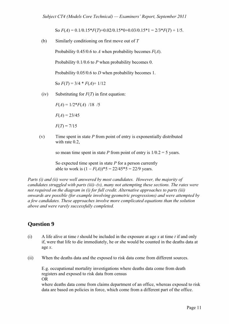
Subject CT4 (Models Core Technical) — Examiners’ Report, September 2011
Page 11
So F(A) = 0.1/0.15*F(T)+0.02/0.15*0+0.03/0.15*1 = 2/3*F(T) + 1/5.
(b) Similarly conditioning on first move out of T
Probability 0.45/0.6 to A when probability becomes F(A).
Probability 0.1/0.6 to P when probability becomes 0.
Probability 0.05/0.6 to D when probability becomes 1.
So F(T) = 3/4 * F(A)+ 1/12
(iv) Substituting for F(T) in first equation:
F(A) = 1/2*F(A) /18 /5 F(A) = 23/45 F(T) = 7/15 (v) Time spent in state P from point of entry is exponentially distributed
with rate 0.2,
so mean time spent in state P from point of entry is 1/0.2 = 5 years.
So expected time spent in state P for a person currently able to work is (1 − F(A))*5 = 22/45*5 = 22/9 years.
Parts (i) and (ii) were well answered by most candidates. However, the majority of candidates struggled with parts (iii)–(v), many not attempting these sections. The rates were not required on the diagram in (i) for full credit. Alternative approaches to parts (iii) onwards are possible (for example involving geometric progressions) and were attempted by a few candidates. These approaches involve more complicated equations than the solution above and were rarely successfully completed. Question 9 (i) A life alive at time t should be included in the exposure at age x at time t if and only if, were that life to die immediately, he or she would be counted in the deaths data at age x. (ii) When the deaths data and the exposed to risk data come from different sources. E.g. occupational mortality investigations where deaths data come from death registers and exposed to risk data from census OR where deaths data come from claims department of an office, whereas exposed to risk data are based on policies in force, which come from a different part of the office.
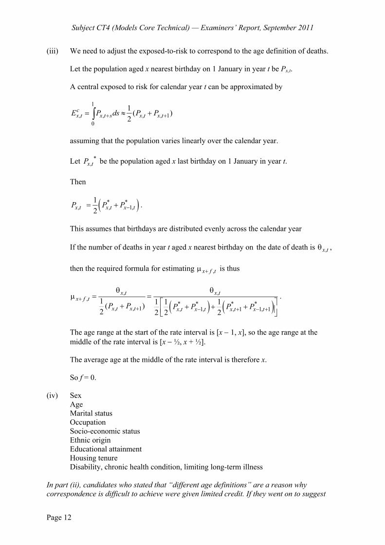
Subject CT4 (Models Core Technical) — Examiners’ Report, September 2011
Page 12
(iii) We need to adjust the exposed-to-risk to correspond to the age definition of deaths. Let the population aged x nearest birthday on 1 January in year t be Px,t.
A central exposed to risk for calendar year t can be approximated by
1
, , , , 10
1 ( )2
cx t x t s x t x tE P ds P P+ += ≈ +∫
assuming that the population varies linearly over the calendar year. Let *
,x tP be the population aged x last birthday on 1 January in year t. Then
( )* *, , 1,
12x t x t x tP P P −= + .
This assumes that birthdays are distributed evenly across the calendar year If the number of deaths in year t aged x nearest birthday on the date of death is ,x tθ , then the required formula for estimating ,x f t+μ is thus
( ) ( )
, ,,
* * * *, , 1 , 1, , 1 1, 1
1 1 1 1( )2 2 2 2
x t x tx f t
x t x t x t x t x t x tP P P P P P+
+ − + − +
θ θμ = =
⎡ ⎤+ + + +⎢ ⎥⎣ ⎦
.
The age range at the start of the rate interval is [x − 1, x], so the age range at the middle of the rate interval is [x − ½, x + ½]. The average age at the middle of the rate interval is therefore x. So f = 0. (iv) Sex Age Marital status Occupation Socio-economic status Ethnic origin Educational attainment Housing tenure Disability, chronic health condition, limiting long-term illness In part (ii), candidates who stated that “different age definitions” are a reason why correspondence is difficult to achieve were given limited credit. If they went on to suggest
Subject CT4 (Models Core Technical) — Examiners’ Report, September 2011
Page 13
that different age definitions can arise because the deaths data and the exposed-to-risk data come from different sources, and gave a relevant example, full credit was awarded. Many candidates, however, did not describe the different age definitions clearly. Part (iii) was better answered than have been exposed-to-risk questions in recent examination papers. In part (iv) “smoking behaviour” is NOT correct as a factor which a national statistical office might use to classify mortality, neither are factors such as “type of policy”, “policy size” or “sales channel”. Candidates are reminded to read the question carefully! Question 10 (i) Outliers. Since all the information is summarised in one number, a few large deviations may be offset or hidden by a large number of small deviations. Small bias. Since the squares of the differences are used, the sign of the differences are lost, hence small but consistent bias above or below may not be noticed. Clumps or runs. Again because the squares of the differences are used, the sign of the
differences are lost, so significant groups of (clumps or runs) of bias over ranges of the data may not be detected.
(ii) (a) A few large deviations or outliers – Individual Standardised Deviations Test. Small but consistent bias – Signs Test OR Cumulative Deviations Test. Clumps or runs of bias over ranges of the data - Grouping of Signs Test OR Serial Correlations Test. (b) Individual Standardised Deviations Test Under the null hypothesis that the standard table rates OR graduated
rates are the true rates underlying the observed data we would expect individual deviations to be distributed Normal (0,1).
EITHER only 1 in 20 zx should lie above 1.96 in absolute value
OR none should lie above 3 in absolute value OR table (see below) showing split of deviations, actual versus expected. ( , 2)−∞ − (−2, −1) (−1, 0) (0, 1) (1, 2) ( 2,+∞ ) Expected 0.22 1.54 3.74 3.74 1.54 0.22 Observed 0 0 5 4 1 1
The largest deviation we have here is 3.31. This is well outside the range −1.96 to 1.96 so we have reason to reject the
null hypothesis.
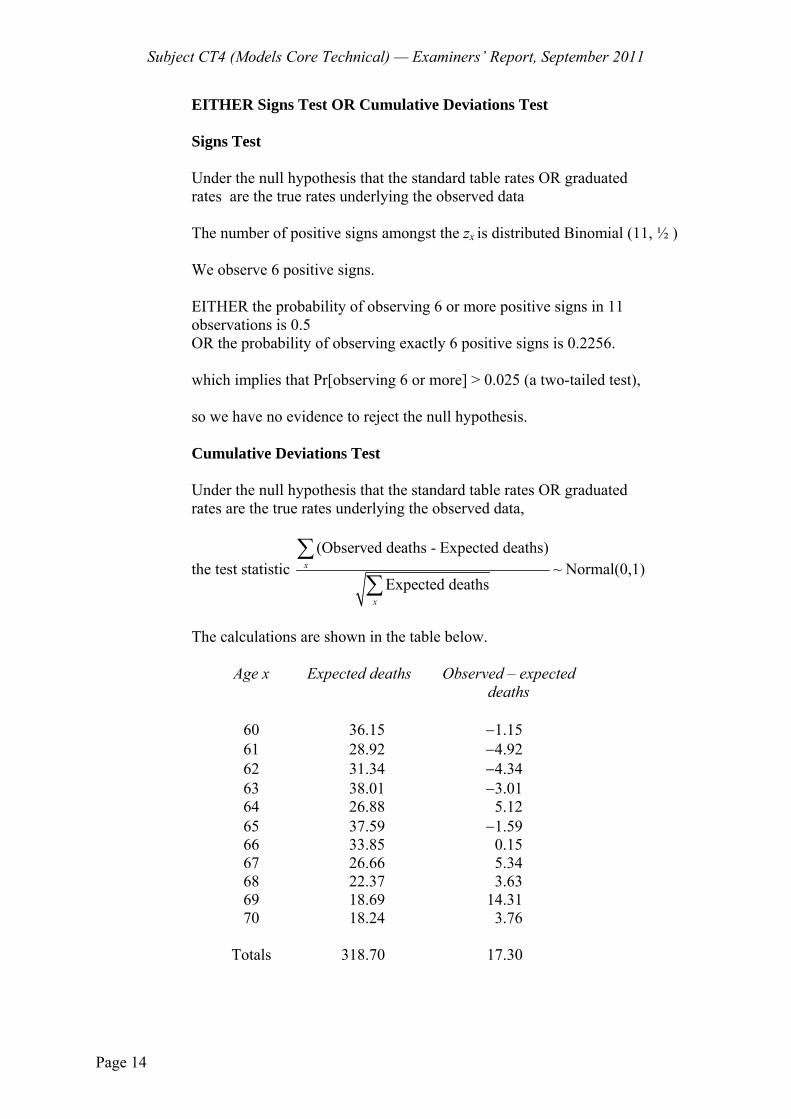
Subject CT4 (Models Core Technical) — Examiners’ Report, September 2011
Page 14
EITHER Signs Test OR Cumulative Deviations Test
Signs Test Under the null hypothesis that the standard table rates OR graduated
rates are the true rates underlying the observed data The number of positive signs amongst the zx is distributed Binomial (11, ½ )
We observe 6 positive signs.
EITHER the probability of observing 6 or more positive signs in 11
observations is 0.5 OR the probability of observing exactly 6 positive signs is 0.2256.
which implies that Pr[observing 6 or more] > 0.025 (a two-tailed test),
so we have no evidence to reject the null hypothesis. Cumulative Deviations Test Under the null hypothesis that the standard table rates OR graduated rates are the true rates underlying the observed data,
the test statistic (Observed deaths - Expected deaths)
Expected deathsx
x
∑∑
~ Normal(0,1)
The calculations are shown in the table below. Age x Expected deaths Observed – expected deaths 60 36.15 −1.15 61 28.92 −4.92 62 31.34 −4.34 63 38.01 −3.01 64 26.88 5.12 65 37.59 −1.59 66 33.85 0.15 67 26.66 5.34 68 22.37 3.63 69 18.69 14.31 70 18.24 3.76 Totals 318.70 17.30

Subject CT4 (Models Core Technical) — Examiners’ Report, September 2011
Page 15
The value of the test statistic is 17.30 0.969318.70
=
and, since – 1.96 < test statistic < +1.96 we have insufficient evidence to reject the null hypothesis.
EITHER Grouping of Signs Test OR Serial Correlations Test Grouping of Signs Test
Under the null hypothesis that the standard table rates OR the graduated rates are the true rates underlying the observed data G = Number of groups of positive deviations = 2 m = number of deviations = 11 n1 = number of positive deviations = 6 n2 = number of negative deviations = 5 THEN EITHER We want k* the largest k such that
1 2
1
1 11
10.05
n nk
t tm
t n
− +⎛ ⎞⎛ ⎞⎜ ⎟⎜ ⎟−⎝ ⎠⎝ ⎠
⎛ ⎞= ⎜ ⎟
⎝ ⎠
<∑
The test fails at the 5% level if G ≤ k*. From the Gold Book k* = 1. So we have insufficient evidence to reject the null hypothesis. OR For t = 2
1 21 5 1 65 and 15
1 1 2n nt t− +⎛ ⎞ ⎛ ⎞ ⎛ ⎞ ⎛ ⎞
= = = =⎜ ⎟ ⎜ ⎟ ⎜ ⎟ ⎜ ⎟−⎝ ⎠ ⎝ ⎠ ⎝ ⎠ ⎝ ⎠
1
11and 462
6mn⎛ ⎞ ⎛ ⎞
= =⎜ ⎟ ⎜ ⎟⎝ ⎠⎝ ⎠
So Pr[t = 2] if the null hypothesis is true is 75/462 = 0.162, which is greater than 5% so we have insufficient evidence reject the null hypothesis.
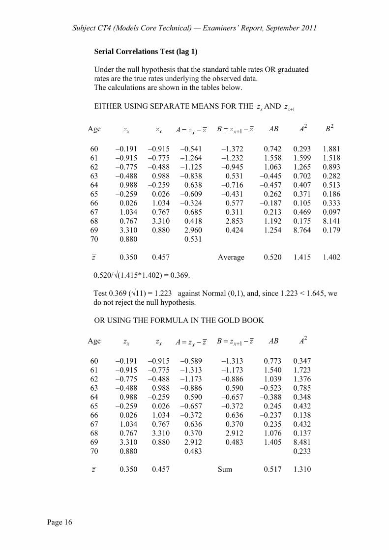
Subject CT4 (Models Core Technical) — Examiners’ Report, September 2011
Page 16
Serial Correlations Test (lag 1) Under the null hypothesis that the standard table rates OR graduated
rates are the true rates underlying the observed data. The calculations are shown in the tables below. EITHER USING SEPARATE MEANS FOR THE xz AND 1xz +
Age zx zx xA z z= − 1xB z z+= − AB 2A 2B
60 –0.191 –0.915 –0.541 –1.372 0.742 0.293 1.881 61 –0.915 –0.775 –1.264 –1.232 1.558 1.599 1.518 62 –0.775 –0.488 –1.125 –0.945 1.063 1.265 0.893 63 –0.488 0.988 –0.838 0.531 –0.445 0.702 0.282 64 0.988 –0.259 0.638 –0.716 –0.457 0.407 0.513 65 –0.259 0.026 –0.609 –0.431 0.262 0.371 0.186 66 0.026 1.034 –0.324 0.577 –0.187 0.105 0.333 67 1.034 0.767 0.685 0.311 0.213 0.469 0.097 68 0.767 3.310 0.418 2.853 1.192 0.175 8.141 69 3.310 0.880 2.960 0.424 1.254 8.764 0.179 70 0.880 0.531 z 0.350 0.457 Average 0.520 1.415 1.402
0.520/√(1.415*1.402) = 0.369. Test 0.369 (√11) = 1.223 against Normal (0,1), and, since 1.223 < 1.645, we
do not reject the null hypothesis. OR USING THE FORMULA IN THE GOLD BOOK
Age zx zx xA z z= − 1xB z z+= − AB 2A 60 –0.191 –0.915 –0.589 –1.313 0.773 0.347 61 –0.915 –0.775 –1.313 –1.173 1.540 1.723 62 –0.775 –0.488 –1.173 –0.886 1.039 1.376 63 –0.488 0.988 –0.886 0.590 –0.523 0.785 64 0.988 –0.259 0.590 –0.657 –0.388 0.348 65 –0.259 0.026 –0.657 –0.372 0.245 0.432 66 0.026 1.034 –0.372 0.636 –0.237 0.138 67 1.034 0.767 0.636 0.370 0.235 0.432 68 0.767 3.310 0.370 2.912 1.076 0.137 69 3.310 0.880 2.912 0.483 1.405 8.481 70 0.880 0.483 0.233 z 0.350 0.457 Sum 0.517 1.310

Subject CT4 (Models Core Technical) — Examiners’ Report, September 2011
Page 17
1 (5.617)10 0.3951 (14.405)11
= .
Test 0.395 (√11) = 1.309 against Normal (0,1), and, since 1.309 < 1.645, we
do not reject the null hypothesis.
(iii) The result of the Individual Standard Deviation test suggests outliers in the data. The actual and expected deaths are relatively low, suggesting that the population in the rural area is not very large. The ages under consideration are also high, exacerbating this scarcity of data.
However there are at least five (actual/expected) deaths in each age group, so the data are adequate.
So this is unlikely to account for the outlier at age 69 years, which should be
investigated further.
The period of the observation is not stated and could affect the results, as, for example if the observation only covered one winter a particularly bad influenza epidemic may have caused more deaths than usual (although this would likely impact all ages in this range similarly). Both the signs and grouping of signs test suggest no bias over the whole or part of the data. However there does seem to be a drift towards the number of observed deaths exceeding the expected at higher ages, and the number observed being smaller than expected at younger ages. Perhaps if a larger extract from the investigation were considered or the
table in its entirety, bias may be observed. Answers to this question were disappointing. Too many answers to part (i) were sketchy and failed to explain WHY the chi-squared test sometimes fails to detect small bias, outliers or “runs” of deviations of the same sign. In part (ii) some candidates failed to relate the tests they were performing to the deficiencies of the chi-squared test identified in part (i); other candidates performed two tests for the same deficiency (only the higher scoring of which received credit). Many candidates lost marks for vagueness in the execution of the tests. Although not all the points listed above were required in part (iii) for full credit, the number of marks available indicated that candidates were expected to go beyond the basic results of the tests. Disappointingly few did this.
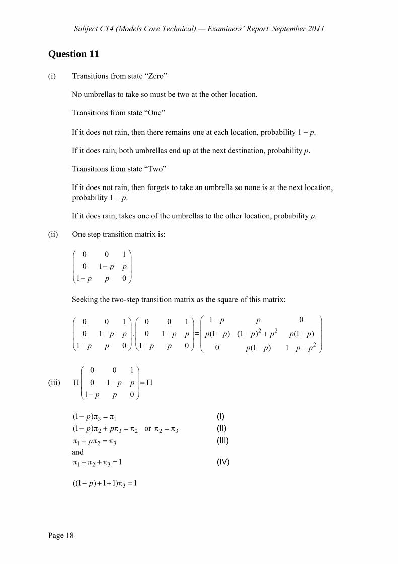
Subject CT4 (Models Core Technical) — Examiners’ Report, September 2011
Page 18
Question 11 (i) Transitions from state “Zero”
No umbrellas to take so must be two at the other location.
Transitions from state “One”
If it does not rain, then there remains one at each location, probability 1 − p.
If it does rain, both umbrellas end up at the next destination, probability p. Transitions from state “Two” If it does not rain, then forgets to take an umbrella so none is at the next location, probability 1 − p. If it does rain, takes one of the umbrellas to the other location, probability p.
(ii) One step transition matrix is:
0 0 10 1
1 0p p
p p
⎛ ⎞⎜ ⎟−⎜ ⎟⎜ ⎟−⎝ ⎠
Seeking the two-step transition matrix as the square of this matrix:
0 0 10 1
1 0p p
p p
⎛ ⎞⎜ ⎟−⎜ ⎟⎜ ⎟−⎝ ⎠
.0 0 10 1
1 0p p
p p
⎛ ⎞⎜ ⎟−⎜ ⎟⎜ ⎟−⎝ ⎠
= 2 2
2
1 0
(1 ) (1 ) (1 )
0 (1 ) 1
p p
p p p p p p
p p p p
−⎛ ⎞⎜ ⎟
− − + −⎜ ⎟⎜ ⎟− − +⎝ ⎠
(iii) 0 0 10 1
1 0p p
p p
⎛ ⎞⎜ ⎟Π − = Π⎜ ⎟⎜ ⎟−⎝ ⎠
3 1(1 )p− π = π (I)
2 3 2(1 )p p− π + π = π or 2 3π = π (II)
1 2 3pπ + π = π (III) and
1 2 3 1π + π + π = (IV)
3((1 ) 1 1) 1p− + + π =
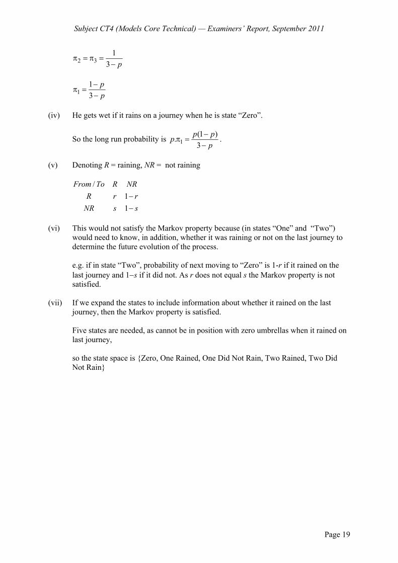
Subject CT4 (Models Core Technical) — Examiners’ Report, September 2011
Page 19
2 31
3 pπ = π =
−
113
pp
−π =
−
(iv) He gets wet if it rains on a journey when he is state “Zero”.
So the long run probability is 1(1 ).3
p ppp
−π =
−.
(v) Denoting R = raining, NR = not raining
/11
From To R NRR r r
NR s s−−
(vi) This would not satisfy the Markov property because (in states “One” and “Two”) would need to know, in addition, whether it was raining or not on the last journey to determine the future evolution of the process. e.g. if in state “Two”, probability of next moving to “Zero” is 1-r if it rained on the last journey and 1−s if it did not. As r does not equal s the Markov property is not satisfied. (vii) If we expand the states to include information about whether it rained on the last journey, then the Markov property is satisfied. Five states are needed, as cannot be in position with zero umbrellas when it rained on last journey, so the state space is {Zero, One Rained, One Did Not Rain, Two Rained, Two Did Not Rain}
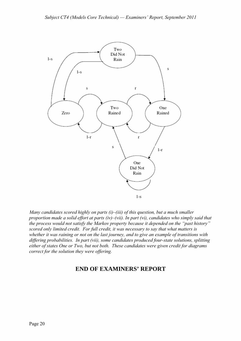
Subject CT4 (Models Core Technical) — Examiners’ Report, September 2011
Page 20
Many candidates scored highly on parts (i)–(iii) of this question, but a much smaller proportion made a solid effort at parts (iv)–(vii). In part (vi), candidates who simply said that the process would not satisfy the Markov property because it depended on the “past history” scored only limited credit. For full credit, it was necessary to say that what matters is whether it was raining or not on the last journey, and to give an example of transitions with differing probabilities. In part (vii), some candidates produced four-state solutions, splitting either of states One or Two, but not both. These candidates were given credit for diagrams correct for the solution they were offering.
END OF EXAMINERS’ REPORT
Related Documents

![[XLS] · Web view2011 1/3/2011 1/3/2011 1/5/2011 1/7/2011 1/7/2011 1/7/2011 1/7/2011 1/7/2011 1/7/2011 1/7/2011 1/7/2011 1/7/2011 1/11/2011 1/11/2011 1/11/2011 1/11/2011 1/11/2011](https://static.cupdf.com/doc/110x72/5b3f90027f8b9aff118c4b4e/xls-web-view2011-132011-132011-152011-172011-172011-172011-172011.jpg)


![[XLS] Object Summary.xlsx · Web view5/26/2010 5/26/2010. 5/2/2011 5/2/2011. 9/30/2011 9/30/2011. 7/6/2011 7/6/2011. 11/28/2011 11/28/2011. 12/6/2011 12/6/2011. 11/28/2011 11/28/2011.](https://static.cupdf.com/doc/110x72/5ae744ba7f8b9a87048f0cd5/xls-object-summaryxlsxweb-view5262010-5262010-522011-522011-9302011.jpg)