Corrected trapezoidal rules for a class of singular …olofr/Publications/gentrap.pdf · Corrected trapezoidal rules for a class of singular ... and Chen designed singularity-corrected

IMA Journal of Numerical Analysis (2013) Page 1 of 32doi:10.1093/imanum/drt046

Corrected trapezoidal rules for a class of singular functions

Oana Marin∗

Department of Mathematics, KTH, 100 44, Stockholm, Sweden, currently Mathematics and ComputerScience, ANL, IL 60439, USA

∗Corresponding author: [email protected]

and

Olof Runborg and Anna-Karin Tornberg

Department of Mathematics and Swedish e-Science Research Center (SeRC), KTH, 100 44,Stockholm, Sweden

[email protected] [email protected]

[Received on 29 January 2013; revised on 29 January 2013]

A set of accurate quadrature rules applicable to a class of integrable functions with isolated singularitiesis designed and analysed theoretically in one and two dimensions. These quadrature rules are basedon the trapezoidal rule with corrected quadrature weights for points in the vicinity of the singularity. Tocompute the correction weights, small-size ill-conditioned systems have to be solved. The convergence ofthe correction weights is accelerated by the use of compactly supported functions that annihilate boundaryerrors. Convergence proofs with error estimates for the resulting quadrature rules are given in both oneand two dimensions. The tabulated weights are specific for the singularities under consideration, but themethodology extends to a large class of functions with integrable isolated singularities. Furthermore, inone dimension we have obtained a closed form expression based on which the modified weights can becomputed directly.

Keywords: singular functions; quadrature methods; high order.

1. Introduction

This paper focuses on the design of accurate quadrature rules for functions with isolated singularities.The need to numerically evaluate such integrals arises in, e.g., methods based on boundary integralequations, where the fundamental solution, or Green’s function, has an integrable singularity.

In the literature one can find several different approaches to the numerical integration of singularfunctions. These include different semianalytical techniques and singularity subtraction approaches (seePozrikidis, 1992). Different mappings and changes of coordinates in order to remove the singularityhave also been applied (see Duffy, 1982; Bruno & Kunyansky, 2001; Atkinson, 2004; Khayat & Wilton,2005; Sidi, 2005; Mousavi & Sukumar, 2010). The approach that we will follow here is to modify thetrapezoidal rule to render it high-order accurate for singular functions. The resulting quadrature rulesare very attractive due to their simplicity—the trapezoidal rule is modified with a small number ofcorrection weights, and the simple structure is retained.

The trapezoidal rule is spectrally accurate for smooth, compactly supported or periodic functions.For other functions it is in general at most second-order accurate. There are two sources of theselarger errors: singularities and boundaries. Both of these error sources can be reduced by modifyingthe quadrature weights locally, in the vicinity of the singularity (which is assumed here to be isolated)

c© The authors 2013. Published by Oxford University Press on behalf of the Institute of Mathematics and its Applications. All rights reserved.

IMA Journal of Numerical Analysis Advance Access published November 14, 2013 at K

TH

Royal Institute of T

echnology on Decem

ber 12, 2013http://im

ajna.oxfordjournals.org/D

ownloaded from

http://imajna.oxfordjournals.org/


2 of 32 O. MARIN ET AL.

or at the boundaries. Hence, by adjusting the weights locally, high-order-accurate versions of the trape-zoidal rule can be constructed also in the presence of singularities and boundaries. The new weightsare precomputed and tabulated; once constructed, the modified trapezoidal rule can easily be applied.In the case of a singularity, the modified weights are, however, specific to the singularity that is beingconsidered.

The first singularity-corrected trapezoidal methods introduced in Rokhlin (1990) were restricted inpractice to rather low orders of accuracy since the magnitude of the correction weights became verylarge for higher-order methods. To alleviate this problem, Alpert (1995) used more correction weightsthan the optimal number, and minimized their sum of squares. The integration interval is split at thesingularity into two subintervals such that the singularity is always at a boundary. Kapur & Rokhlin(1997) introduced additional quadrature points and weights outside the interval of integration and couldthereby obtain much smaller correction weights. Such a method is not always convenient to apply, andyet another approach by Alpert (1999), was to introduce a hybrid Gauss–trapezoidal rule, where a fewof the regularly spaced nodes towards the interval end points are replaced with irregularly spaced nodes.The computed weights at the irregular nodes are both bounded and positive.

In the papers Rokhlin (1990), Alpert (1995, 1999) and Kapur & Rokhlin (1997), quadrature rulesare designed for singular functions of the form f (x)= φ(x)s(x)+ ψ(x) and f (x)= φ(x)s(x), whereφ(x) and ψ(x) are regular functions and s(x) has an isolated integrable singularity such as s(x)= |x|γ ,γ >−1 or s(x)= log(|x|). The integration interval is split at the singularity, and for each subintervalthere is a regular end and a singular end. Corrections to the trapezoidal rule are applied at both ends inorder to reduce the boundary errors at the regular end and to control the error from the singularity andthe boundary at the other end. Theoretical analysis is offered for all these methods.

It is inconvenient to split the domain of integration at the singularity in higher dimensions. Aguilarand Chen designed singularity-corrected trapezoidal rules for the s(x)= log(|x|) singularity in R

2 (seeAguilar & Chen, 2002), and for s(x)= 1/|x| in R

3 (see Aguilar & Chen, 2005). The singularities areinterior to the domain and a singularity correction in the interior is combined with boundary correctionsto yield higher-order methods. No theoretical analysis is provided in these papers, but the expected orderof accuracy is given for the method, which is consistent with numerical examples.

One procedure for constructing a set of increasingly accurate quadrature rules is to require the exactintegration of monomials of increasing degree (see Keast & Lyness, 1979). A similar procedure isfollowed here to determine the modified weights of the corrected trapezoidal rules. The exact integrationof monomials, up to a desired degree, multiplying the singular function s(x) is first enforced for aspecific uniform grid spacing h. This leads to a linear system of equations for the modified weights.The obtained correction weights will then depend on h. This is not very practical. Instead, one wantsto use the converged weights that are defined as the weights obtained in the limit as h → 0. They aregrid independent, universal for the given singularity and can be tabulated once computed. As Aguilar &Chen (2002, 2005) note, the system to be solved for the weights becomes severely ill conditioned, moreso for smaller h and multiprecision arithmetic is needed to perform this task.

Duan & Rokhlin (2009) apply similar techniques to design singularity-corrected trapezoidal rulesfor s(x)= log(|x|) singularities in two dimensions. However, they do not seek converged correctionweights, but compute weights that depend on the grid size h. They are able to derive analytical, althoughvery lengthy, expressions for the weights and thereby avoid solving an ill-conditioned system. Theanalytical formulas that they derive are, however, approximated numerically, but to very high accuracy.A theoretical proof is offered regarding the accuracy of the quadrature rules, using also some theoreticalresults developed in Lyness (1976).

at KT

H R

oyal Institute of Technology on D

ecember 12, 2013


Dow

nloaded from



CORRECTED TRAPEZOIDAL RULES FOR A CLASS OF SINGULAR FUNCTIONS 3 of 32

In this paper we consider singularities of the kind s(x)= |x|γ , γ >−1 in one dimension and s(x)=1/|x| in two dimensions. The singularities are interior to the domain. As in Aguilar & Chen (2002),our singularity corrections can be combined with boundary corrections (see Alpert, 1995) to reduceboundary errors as needed.

One difference in our approach compared with all previous works cited above lies in the procedurefor computing the weights. The corrected trapezoidal rule is based on the punctured trapezoidal rule(excluding the point of singularity) together with a correction operator which is applied at grid pointsin the vicinity of the singularity. In order to accelerate the convergence of the weights, the boundaryerrors in the punctured trapezoidal rule must be reduced. The approach used previously is to introducea boundary correction for the trapezoidal rule. Here, we suggest an alternative approach where wemultiply s(x) by a fixed, compactly supported function g(x). This completely annihilates the boundaryerrors. The convergence rate of the weights will now instead depend on the number of derivatives ofg that vanish at the point of singularity. This is proved for the one-dimensional case in Section 3; seeLemma 3.8. For the two-dimensional case, we cannot offer a rigorous proof, but note the same behaviourin practice. With a faster convergence rate for the weights, larger values of h can be used, which to someextent reduces the ill conditioning of the system. To compute converged weights to double precision,we use a multiprecision library that allows for computations in multiprecision arithmetic.

In the one-dimensional case we are able to show that the converged weights are the solution to alinear system of equations, where the system matrix is a Vandermonde matrix and where the right-handside has an analytic expression in terms of the Riemann zeta function (see the Appendix). Hence, in thiscase, we can directly compute the converged weights by solving this system of equations.

The singularity corrections that we design are of order O(h2+γ+d+2p) in Rd , d = 1, 2 as weights are

modified at grid points in p layers around the singularity; see Theorem 3.7. In two dimensions (γ = −1),for p = 0, which corresponds to a single correction weight at the singularity, we have a third-orderrule. For each additional layer of correction weights, the order of accuracy increases by 2. Comparedwith Aguilar & Chen (2002) our layers differ somewhat, with the number of correction weights in ourapproach growing more slowly as the number of layers is increased. We also have a theoretical analysisof the method’s convergence rate.

In two dimensions, we have considered the singularity 1/|x|, which is the Green’s function for theLaplace equation in three dimensions, instead of log(|x|) as in Aguilar & Chen (2002) and Duan &Rokhlin (2009). A boundary integral equation for the three-dimensional Laplace equation contains inte-grals over two-dimensional surfaces that are the boundaries of the domain. This method would applywhen the boundary is flat. Extensions based on the approach and the theory presented in this paper arediscussed in the conclusions.

The outline of the paper is as follows. In Section 2, we describe the modified trapezoidal rulesand their structure and we define the system of equations from which the correction weights can beobtained. The theoretical analysis is presented in Section 3, starting with the accuracy of the puncturedtrapezoidal rule, before we prove the accuracy of the modified trapezoidal rules. We also give a proofof convergence for the correction weights in one dimension. Numerical results to validate the con-structed quadrature rules together with discussions concerning implementation aspects are provided inSection 4.

1.1 Notation

In order to render the text more legible, multiindex notation will be used. A multiindex in thed-dimensional set-up is α = (α1, . . . ,αd). For α ∈ R

d , Zd , including multiindices, we define the norms

at KT

H R


ecember 12, 2013


Dow

nloaded from




|α| = ∑di=1 |αi| and |α|2 =

√∑di=1 α

2i . To be more explicit we write at times |α|1 instead of |α|. We also

use α! = α1! · · ·αd !. For x ∈ Rd we define monomials xα = xα1

1 · · · xαdd and for the partial derivatives,

∂αf (x)= ∂ |α|

∂xα11 · · · ∂xαd

d

f (x).

Occasionally, we will make use of the basis vectors in Rd which shall be denoted by ei with

1 � i � d.The notation [x] for the integer part of x and {x} for the fractional part of x will also be used;

recall that x = [x] + {x}. Throughout the manuscript C will denote a constant which is independent ofother parameters relevant in the particular context where it is used, typically the grid spacing h andposition x. It may at times be accompanied by a numeric subscript to differentiate it from other similarconstants.

1.2 Trapezoidal rule

Consider a function f ∈ C2p+2(Rd), defined on the interval S = [−a, a] for d = 1, and on the squareS = [−a, a]2 for d = 2. The standard trapezoidal rule in one dimension is then given by

∫S

f (x) dx ≈ Th[f ] :=N∑

β=−N

hf (βh)− 1

2(hf (a)+ hf (−a)), h = a/N (1.1)

and in two dimensions, with the same h, by

∫S

f (x) dx ≈ Th[f ] :=∑βh∈Sβ∈Z

2

h2f (βh)− 1

2

∑βh∈∂Sβ∈Z

2

h2f (βh)− 1

4

∑βh∈∂Sc

β∈Z2

h2f (βh), (1.2)

where we used ∂Sc to denote the four corner points of S. Typically, for a smooth integrand over abounded interval, numerical integration using the trapezoidal rule exhibits second-order convergence.To delve further into the error analysis of the trapezoidal rule, and later the modified trapezoidal rule,we will use two main approaches: the Euler–Maclaurin expansion and Fourier analysis. We use thefollowing precise form of the Euler–Maclaurin expansion.

Theorem 1.1 (Euler–Maclaurin expansion) For a function f ∈ C2p+2([a, b]),

∫ b

af (x) dx = Th[f ] +

p∑�=1

h2�b2�

(2�)!(f (2�−1)(b)− f (2�−1)(a))

+ h2p+2

(2p + 2)!

∫ b

aB2p+2

({x − a

h

})f (2p+2)(x) dx. (1.3)

The expression uses the Bernoulli polynomials Bp and the Bernoulli numbers defined as bp = Bp(0).The periodized versions Bp({x}) are piecewise smooth and bounded functions detailed in Cohen (2007,Proposition 9.3.1 and Remark 2).

at KT

H R


ecember 12, 2013


Dow

nloaded from




From the Euler–Maclaurin expansion (1.3) we see that there are two main sources of error in thetrapezoidal rule, corresponding to the terms in the error expression. First, we have the contribution tothe error from the boundaries given by

p∑�=1

h2�b2�

(2�)!(f (2�−1)(b)− f (2�−1)(a)). (1.4)

Second, we have the contribution of the error which is determined by the regularity of the function,

h2p+2

(2p + 2)!

∫ b

aB2p+2

({x − a

h

})f (2p+2)(x) dx.

There are two common situations when the sum in (1.4) vanishes for integrands of class C2p+2(R):when the integrand is periodic on [a, b] and when the integrand is compactly supported within (a, b). Inthis case the error of the trapezoidal rule is O(h2p+2). If the integrand is C∞ and there are no boundaryerrors, the trapezoidal rule exhibits spectral convergence.

The accuracy of the trapezoidal rule may also be studied through Fourier analysis. In this approachwe use the Poisson summation formula for f ∈ C2

c (R) and note that

Th[f ] =∑

j

hf (jh)=∑

k

f

(k

h

)=

∫f (x) dx +

∑k |= 0

f

(k

h

),

where

f (k)=∫

f (x) e−2π ikx dx. (1.5)

Our aim is to show that this oscillatory integral can be estimated by

|f (k)| � C

|k|p , p> 1,

from which it will then follow that∣∣∣∣Th[f ] −∫

f (x) dx

∣∣∣∣ �∑k |= 0

∣∣∣∣f(

k

h

)∣∣∣∣ � Chp∑k |= 0

1

|k|p � C′hp.

2. Modified trapezoidal rules

We will construct modified trapezoidal rules with a singularity correction for functions with isolatedsingularities. More precisely, we consider functions f (x)= s(x)φ(x) where φ(x) is regular and

s(x)= |x|γ with

{γ ∈ (−1, 0), x ∈ R,

γ = −1, x ∈ R2.

(2.1)

at KT

H R


ecember 12, 2013


Dow

nloaded from




2.1 Simple correction

Let us define the punctured trapezoidal rule, as applied to a compactly supported function f :

T0h [f ] =

∑β |= 0

hdf (βh), β ∈ Zd . (2.2)

Introduce the simply corrected quadrature rule Q0h[φ · s] = T0

h [φ · s] + a(h)ω0φ(0), where a(h) is aweight factor depending on the singularity and it is known beforehand. The correction weight ω0(h)is defined by

a(h)ω0(h)g(0)=∫

g(x)s(x) dx − T0h [g · s], (2.3)

where g(x) is a compactly supported function with g(x) |= 0. The function g(x) is introduced to annihilatethe boundary errors from the punctured trapezoidal rule.

If the weight factor a(h) is chosen correctly, then ω0(h)→ ω0 as h → 0 where ω0 does not dependon h nor on g. The convergence rate of ω0(h)→ ω0, however, depends strongly on the choice of g.Convergence is fast when the function g is flat at the singularity, i.e., it has several derivatives thatvanish at the origin; see Section 4.

The modified quadrature rule reads

Q0h[φ · s] = T0

h [φ · s] + a(h)ω0φ(0), (2.4)

where for a space of dimension d,a(h)= hds(h)= hγ+d . (2.5)

We will show below that adding a modification at the origin in this way will lead to a method oforder O(h2+d+γ ) for s(x) given by (2.1). This assumes that the function φ(x) is regular enough, andalso compactly supported within the integration domain. If it is not compactly supported, T0

h should bereplaced by a boundary-corrected punctured trapezoidal rule (see Alpert, 1995).

2.2 Higher-order correction

A higher-order quadrature rule will involve more correction weights. Define

Qph[φ · s] = T0

h [φ · s] + a(h)∑β∈Lp

ωβφ(βh), (2.6)

whereLp = {β ∈ Z

d s.t. |β|1 � p}. (2.7)

In analogy with (2.3), the weights should satisfy the following equations:∫g(x)s(x)x2α dx = T0

h [g · s · x2α] + a(h)∑β∈Lp

ωβ(h)(βh)2αg(βh) ∀α s.t. |α|1 � p. (2.8)

Temporarily denote the weight associated with a point (xi, yj) (β = (i, j)) by wi,j. We then requirew±i,±j = w±j,±i for all possible combinations of signs. Such a weight will be denoted by wm

q , whereq = |i| + |j|, and m will be defined below. Due to these symmetry assumptions for the weights, theequations in (2.8) are stated only for even-order monomials since the equations for odd monomials

at KT

H R


ecember 12, 2013


Dow

nloaded from




p=1 p=2 p=3

β1

β 2

−4 −3 −2 −1 0 1 2 3 4

−3

−2

−1

0

1

2

3

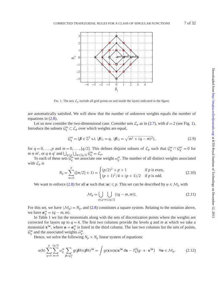
Fig. 1. The sets Lp include all grid points on and inside the layers indicated in the figure.

are automatically satisfied. We will show that the number of unknown weights equals the number ofequations in (2.8).

Let us now consider the two-dimensional case. Consider sets Lp as in (2.7), with d = 2 (see Fig. 1).Introduce the subsets Gm

q ⊂Lp over which weights are equal,

Gmq = {β ∈ Z

2 s.t. |β|1 = q, |β|2 =√

m2 + (q − m)2}, (2.9)

for q = 0, . . . , p and m = 0, . . . , [q/2]. This defines disjoint subsets of Lp such that Gmq ∩ Gm′

q′ = 0 form |= m′, or q |= q′ and

⋃q�p

⋃m�[q/2] Gm

q =Lp.To each of these sets Gm

q we associate one weight ωmq . The number of all distinct weights associated

with Lp is

Np =p∑

m=0

([m/2] + 1)={(p/2)2 + p + 1 if p is even,

(p + 1)2/4 + (p + 1)/2 if p is odd.(2.10)

We want to enforce (2.8) for all α such that |α| � p. This set can be described by α ∈Mp with

Mp =⋃q�p

⋃m�[q/2]

{(q − m, m)}. (2.11)

For this set, we have |Mp| = Np, and (2.8) constitutes a square system. Relating to the notation above,we have αm

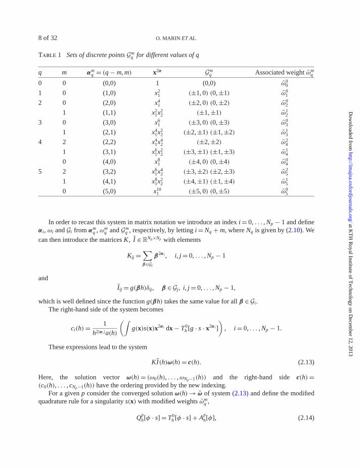
q = (q − m, m).In Table 1 we list the monomials along with the sets of discretization points where the weights are

corrected for layers up to q = 4. The first two columns provide the levels q and m at which we take amonomial x2α , where α = αm

q is listed in the third column. The last two columns list the sets of points,Gm

q and the associated weights ωmq .

Hence, we solve the following Np × Np linear system of equations:

a(h)p∑

q=0

[q/2]∑m=0

ωmq

∑β∈Gm

q

g(βh)(βh)2α =∫

g(x)s(x)x2α dx − T0h [g · s · x2α] ∀α ∈Mp. (2.12)

at KT

H R


ecember 12, 2013


Dow

nloaded from




Table 1 Sets of discrete points Gmq for different values of q

q m αmq = (q − m, m) x2α Gm

q Associated weight ωmq

0 0 (0,0) 1 (0,0) ω00

1 0 (1,0) x21 (±1, 0) (0, ±1) ω0

1

2 0 (2,0) x41 (±2, 0) (0, ±2) ω0

2

1 (1,1) x21x2

2 (±1, ±1) ω12

3 0 (3,0) x61 (±3, 0) (0, ±3) ω0

3

1 (2,1) x41x2

2 (±2, ±1) (±1, ±2) ω13

4 2 (2,2) x41x4

2 (±2, ±2) ω24

1 (3,1) x61x2

2 (±3, ±1) (±1, ±3) ω14

0 (4,0) x81 (±4, 0) (0, ±4) ω0

4

5 2 (3,2) x61x4

2 (±3, ±2) (±2, ±3) ω25

1 (4,1) x81x2

2 (±4, ±1) (±1, ±4) ω15

0 (5,0) x101 (±5, 0) (0, ±5) ω0

5

In order to recast this system in matrix notation we introduce an index i = 0, . . . , Np − 1 and defineαi, ωi and Gi from αm

q , ωmq and Gm

q , respectively, by letting i = Nq + m, where Nq is given by (2.10). We

can then introduce the matrices K, I ∈ RNp×Np with elements

Kij =∑β∈Gj

β2αi , i, j = 0, . . . , Np − 1

and

Iij = g(βh)δij, β ∈ Gj, i, j = 0, . . . , Np − 1,

which is well defined since the function g(βh) takes the same value for all β ∈ Gi.The right-hand side of the system becomes

ci(h)= 1

h2|αi|a(h)

(∫g(x)s(x)x2αi dx − T0

h [g · s · x2αi ]

), i = 0, . . . , Np − 1.

These expressions lead to the system

KI(h)ω(h)= c(h). (2.13)

Here, the solution vector ω(h)= (ω0(h), . . . ,ωNp−1(h)) and the right-hand side c(h)=(c0(h), . . . , cNp−1(h)) have the ordering provided by the new indexing.

For a given p consider the converged solution ω(h)→ ω of system (2.13) and define the modifiedquadrature rule for a singularity s(x) with modified weights ωm

q ,

Qph[φ · s] = T0

h [φ · s] + Aph[φ], (2.14)

at KT

H R


ecember 12, 2013


Dow

nloaded from




with

Aph[φ] = a(h)

p∑q=0

[q/2]∑m=0

ωmq

∑β∈Gm

q

φ(βh), (2.15)

where Gmq is as in (2.9). The constructed rule Qp

h has accuracy O(h2p+3); see Theorem 3.7.In one dimension the expressions for the sets Lp, Mp greatly simplify since in this context

Np = p + 1 and

Lp = {β ∈ Z, |β| = j, j � p}, Mp = {α ∈ N,α = j, j � p}, Gi = {±i}.

So K ∈ R(p+1)×(p+1) has elements K00 = 1 and otherwise the Vandermonde structure Kij = 2j2i. More-

over, Iij(h)= g(ih)δij. The right-hand-side entries are simply

ci(h) := 1

h2ia(h)

[∫g(x)s(x)x2i dx − T0

h [g · s · x2i]

].

The corrected, punctured trapezoidal rule Qph defined as in (2.14) has the correction operator

Aph[φ] := a(h)

p∑j=0

ωj(φ(jh)+ φ(−jh)). (2.16)

3. Theoretical analysis

The techniques used to prove the accuracy of the modified quadrature rule differ in the one-dimensionalset-up from the two-dimensional one. The Fourier approach is chosen for the lower dimension whilein two dimensions the Euler–Maclaurin formula is applied in each direction. In this analysis, we focuson the errors due to the singularities and the accuracy of the singularity corrections. Therefore, weconsider the integration of f (x)= φ(x)s(x), where φ(x) is compactly supported within the integrationdomain.

To begin with we provide an accuracy result for the punctured trapezoidal rule. Using this resultwe obtain an error estimate of the modified trapezoidal rule in terms of h and the difference ω(h)− ω

in Theorem 3.7, where ω(h)− ω can be made sufficiently small with a proper choice of g so thatit does not alter the asymptotic order. This is proved in the one-dimensional case, where we showthat ω(h)→ ω and also obtain an estimate of |ω(h)− ω|, thus yielding a complete error estimatefor the modified trapezoidal rule in one dimension. In two dimensions, we offer no rigorous proofsfor the convergence of the weights, but note the same behaviour as in one dimension in numericalexperiments.

3.1 Accuracy of the punctured trapezoidal rule

To prove the order of convergence of the constructed quadrature rule we start by deriving an errorestimate for the punctured trapezoidal rule. Theorem 3.1 states the one-dimensional result. The corre-sponding two-dimensional result in Theorem 3.2 is weaker; note that the function f = g · s vanishes atthe origin, thus Th[f ] = T 0

h [f ]. General error estimates of the type below were derived in Lyness (1976).However, those also include the boundary errors and do not cover the cases we are interested in here.

at KT

H R


ecember 12, 2013


Dow

nloaded from




Theorem 3.1 Consider f : R → R given as f = g(x)s(x) where s(x)= |x|γ with γ >−1. Let p and q beintegers such that 0 � p< q and 2q + 1> γ . Take g(x) ∈ C2q+2

c (R)with g(k)(0)= 0 for k = 2, 4, . . . , 2p.Then ∣∣∣∣

∫f (x) dx − T0

h [f ] − g(0)hγ+1c(γ )

∣∣∣∣ � C(h2p+γ+3 + h2q+2),

where c(γ ) depends on γ but is independent of h and g.

We note that if γ > 0 this also gives an estimate for the standard trapezoidal rule since then f (0)= 0and Th[f ] = T0

h [f ]. The proof of this theorem is given in Section 3.1.1. In Lemma A2 in the Appendix,a closed form expression for c(γ ) is given.

Theorem 3.2 Consider f : R2 → R given as f (x)= g(x)s(x)where s(x)= 1/|x|. Let q and p be integers

such that q> p. Take g ∈ C2q+3c (R2) with ∂kg(0)= 0 for all k ∈ N

2 such that |k|< 2p + 2. Then it holdsthat ∣∣∣∣

∫f (x) dx − Th[f ]

∣∣∣∣ � Ch2p+3.

This theorem is proved in Section 3.1.2.

3.1.1 One-dimensional case In this section we prove Theorem 3.1. We begin by introducing a cut-offfunction ψ ∈ C∞ satisfying ψ(x)=ψ(−x) and

ψ(x)={

0, |x| � 12 ,

1, |x| � 1.(3.1)

We then haveT0

h [f ] = Th[fψ(·/h)].Consequently,∫

f (x) dx − T0h [f ] =

∫f (x)(1 − ψ(x/h)) dx +

∫f (x)ψ(x/h) dx − Th[fψ(·/h)], (3.2)

and we can estimate the two parts separately. For the first term we have

∫f (x)(1 − ψ(x/h)) dx =

∫ h

−hg(x)s(x)(1 − ψ(x/h)) dx

= hγ+1∫ 1

−1g(hx)s(x)(1 − ψ(x)) dx, (3.3)

where we have used the definition of ψ in (3.1) and a rescaling of the interval. By the symmetry of ψ(x)and s(x) and the assumption of vanishing derivatives,

∫ 1

−1(g(hx)− g(0))s(x)(1 − ψ(x)) dx =

∫ 1

−1

⎛⎝g(hx)−

2p+1∑j=0

g(j)(0)

j!(hx)j

⎞⎠ s(x)(1 − ψ(x)) dx.

at KT

H R


ecember 12, 2013


Dow

nloaded from




Therefore, after estimating the remainder term in the Taylor expansion of g(x), which is bounded byCh2p+2|x|2p+2,

∣∣∣∣∫ 1

−1(g(hx)− g(0))s(x)(1 − ψ(x)) dx

∣∣∣∣ � Ch2p+2∫ 1

−1|x|γ+2p+2|1 − ψ(x)| dx � Ch2p+2. (3.4)

Define

c1(γ )=∫ 1

−1s(x)(1 − ψ(x)) dx.

Then we obtain from (3.4) and (3.3),

∣∣∣∣∫

f (x)(1 − ψ(x)) dx − g(0)hγ+1c1(γ )

∣∣∣∣ = hγ+1

∣∣∣∣∫ 1

−1(g(hx)− g(0))s(x)(1 − ψ(x)) dx

∣∣∣∣� Ch2p+γ+3. (3.5)

For the second term in (3.2) we can use the strategy based on the Fourier analysis as in Section 1.2for the standard trapezoidal rule applied to f (x)ψ(x/h). Hence, since f (x)ψ(x/h) ∈ C2q+2

c (R) we obtainfrom the Poisson summation formula (1.5),

Th[fψ(·/h)] =∫

f (x)ψ(x/h) dx +∑k |= 0

fψ(k/h, h),

fψ(k, h)=∫

f (x)ψ(x/h) e−2π ikx/h dx.

(3.6)

Moreover, by the symmetry of ψ(x),

fψ(k/h, h)+ fψ(−k/h, h)= 2∫

g(x)s(x)ψ(x/h) cos(2πkx/h) dx

= 2�∫ ∞

0(g(x)+ g(−x))s(x)ψ(x/h) e2π ikx/h dx. (3.7)

We will now use Lemma 3.3 stated and proved below, which provides estimates on oscillatoryintegrals of this type. Since the even derivatives of g(x) are zero up to order 2p at x = 0, all derivativesof g(x)= g(x)+ g(−x) are zero up to order 2p + 1 at x = 0. We can therefore apply Lemma 3.3 to theintegral with 2p + 1 for p and 2q + 2 for q. We obtain

∫ ∞

0(g(x)+ g(−x))s(x)ψ(x/h) e2π ikx/h dx = g(0)W(2πk)hγ+1(2πk)−2(q+1)

+ O(k−2(q+1)(hγ+2p+3 + h2q+2)). (3.8)

at KT

H R


ecember 12, 2013


Dow

nloaded from




Using (3.7) combined with (3.8), an expression for fψ(k/h, h)+ fψ(−k/h, h) is obtained. Rewriting thesum in (3.6) to use this expression, we get

Th[fψ(·/h)] =∫

f (x)ψ(x/h) dx + 2�∞∑

k=1

∫ ∞

0(g(x)+ g(−x))s(x)ψ(x/h) e2π ikx/h dx

=∫

f (x)ψ(x/h) dx + 4g(0)hγ+1�∞∑

k=1

W(2πk)

(2πk)2(q+1)

+ [hγ+2p+3 + h2q+2]∞∑

k=1

O(k−2(q+1))

=∫

f (x)ψ(x/h) dx + g(0)hγ+1c2(γ )+ O(hγ+2p+3 + h2q+2), (3.9)

where

c2(γ )= 4�∞∑

k=1

W(2πk)

(2πk)2(q+1).

Note that this is well defined since q � 0 and W(k) is bounded in k. Using (3.2) we get

∣∣∣∣∫

f (x) dx − T0h (f )− g(0)hγ+1(c1(γ )− c2(γ ))

∣∣∣∣�

∣∣∣∣∫

f (x)(1 − ψ(x/h)) dx − g(0)hγ+1c1(γ )

∣∣∣∣+

∣∣∣∣∫

f (x)ψ(x/h) dx − Th(fψ(·/h))+ g(0)hγ+1c2(γ )

∣∣∣∣ .

The result of Theorem 3.1 now follows from (3.5) and (3.9) with

c(γ )= c1(γ )− c2(γ )=∫ 1

−1s(x)(1 − ψ(x)) dx − 4�

∞∑k=1

W(2πk)

(2πk)2(q+1),

which is independent of h and g(x). It remains to state and prove Lemma 3.3.

Lemma 3.3 Let p and q be integers such that 0 � p< q and h and k are positive real numbers, and γ beany real number. Suppose g(x) ∈ Cq

c with supp g ⊂ [0, L] and g(�)(0)= 0 for �= 1, . . . , p. If q> γ + 1and ψ(x) is as given in (3.1), then there is a function W(k) such that

∣∣∣∣∫ ∞

0ψ(x/h)g(x)xγ eikx/h dx − g(0)W(k)hγ+1k−q

∣∣∣∣ � Cqk−q(hγ+2+p + hq), (3.10)

where W(k) is bounded in k and independent of h and g(x) (but depends on q).

at KT

H R


ecember 12, 2013


Dow

nloaded from




Proof. We let s(x)= xγ and note that |s(j)(x)| � Cxγ−j. Since supp ψ(x/h)g(x)⊂ [h/2, L] ⊂ (0, ∞) wehave, after q integrations by parts,

I(h, k) :=∫ ∞

0ψ(x/h)g(x)s(x) eikx/h dx =

(ih

k

)q ∫ ∞

0

(dq

dxqψ(x/h)g(x)s(x)

)eikx/h dx.

Define W(k) as

W(k)= iq∫ ∞

0

(dq

dxqψ(x)s(x)

)eikx dx. (3.11)

Clearly, W(k) does not depend on h. Moreover, ψ(j)(x) is compactly supported for j � 1 and |s(q)(x)| �xγ−q is integrable because q> γ + 1. Therefore,

|W(k)| �∫ ∞

0|ψ(x)s(q)(x)| dx +

q∑j=1

dq,j

∫ ∞

0|ψ(j)(x)s(q−j)(x)| dx � C,

where dq,j are the binomial coefficients. The estimate is independent of k, showing the boundedness ofW(k). After rescaling the integral we also have

W(k)= iqhq−1∫ ∞

0

(dq

dxqψ(x/h)s(x/h)

)eikx/h dx

= iqhq−1−γ∫ ∞

0

(dq

dxqψ(x/h)s(x)

)eikx/h dx.

Then, with r(x) :=ψ(x/h)g(x),

I(h, k)− g(0)W(k)hγ+1k−q

=(

ih

k

)q ∫ ∞

0

(dq

dxq[r(x)− g(0)ψ(x/h)]s(x)

)eikx/h dx

=(

h

ik

)q q∑j=0

dq,j

∫ ∞

0[r(j)(x)− g(0)h−jψ(j)(x/h)]s(q−j)(x) eikx/h dx. (3.12)

We have the following expression for the derivatives of r(x):

r(j)(x)=

⎧⎪⎪⎨⎪⎪⎩

j∑�=0

dj,�

hj−� ψ(j−�)(x/h)g(�)(x), h/2 � x � h,

g(j)(x), h< x � L,

at KT

H R


ecember 12, 2013


Dow

nloaded from




since ψ(j)(x)≡ 0 for j> 0 and x> h. Let δi,j be the Kronecker delta. Exploiting the facts that ψ(x/h)≡ 0for x< h/2 and ψ(x/h)≡ 1 for x> h we obtain, for 0 � j � q,

∫ ∞

0[r(j)(x)− g(0)h−jψ(j)(x/h)]s(q−j)(x) eikx/h dx

=∫ h

h/2

[j∑

�=0

dj,�

hj−� ψ(j−�)(x/h)g(�)(x)− 1

hjψ(j)(x/h)g(0)

]s(q−j)(x) eikx/h dx

+∫ L

hg(j)(x)s(q−j)(x) eikx/h dx − δ0,jg(0)

∫ ∞

hs(q)(x) eikx/h dx

=j∑

�=0

dj,�

hj−�

∫ h

h/2ψ(j−�)(x/h)[g(�)(x)− δ0,�g(0)]s

(q−j)(x) eikx/h dx

+∫ L

h[g(j)(x)− δ0,jg(0)]s


− δ0,jg(0)∫ ∞

Ls(q)(x) eikx/h dx. (3.13)

We will now use the assumption that g(�)(0)= 0 for 1 � �� p. From Taylor’s theorem we get

|g(j)(x)− g(j)(0)| � |g(p+1)|∞ |x|p+1−j

(p + 1 − j)!= C|x|p+1−j, 0 � j � p,

and therefore also

|g(j)(x)− δ0,jg(0)| � Cxmax(p+1−j,0).

We use this to estimate the integrals in (3.13). First, for 0 � j � q and 0 � �� j,

1

hj−�

∣∣∣∣∫ h

h/2ψ(j−�)(x/h)[g(�)(x)− δ0,�g(0)]s


∣∣∣∣� C

hj−�

∫ h

h/2xmax(p+1−�,0)+γ−q+j dx � Chmax(p+1−�,0)+γ−q+1+�

� Chp+2+γ−q,

where we used the fact that hmax(r,0) � hr when h< 1. Moreover, for the second integral in (3.13),

∣∣∣∣∫ L

h[g(j)(x)− δ0,jg(0)]s


∣∣∣∣� C

∫ L

hxmax(p+1−j,0)+γ−q+j dx � C(hmax(p+1−j,0)+γ−q+j+1 + 1)

� C(hp+2+γ−q + 1).

at KT

H R


ecember 12, 2013


Dow

nloaded from




Finally, for the last integral in (3.13),∣∣∣∣∫ ∞

Ls(q)(x) eikx/h dx

∣∣∣∣ � C∫ ∞

Lxγ−q dx � C,

since q> γ + 1. Together with (3.12) these estimates show that

|I(h, k)− g(0)W(k)hγ+1k−q| � C

(h

k

)q

(hp+2+γ−q + 1)� Ck−q(hγ+2+p + hq).

This proves the lemma. �

3.1.2 Two-dimensional case The Euler–Maclaurin expansion formula is the basis for the theoreticalanalysis in two dimensions. Since it provides an error estimate based on the cancellation and bounded-ness of higher-order derivatives—see (1.1)—we first evaluate the higher-order derivatives of the singu-lar function s(x)= 1/|x|. The concluding result of this subsection is the proof of Theorem 3.2.

Lemma 3.4 The partial derivatives of order k of xα/|x| with x = (x1, x2) are given as

∂k xα

|x| = 1

|x||k|−|α|+1Pk,α

(x|x|

), (3.14)

where Pk,α is a polynomial with deg Pk,α = |k| + |α| in two variables Pk,α(x)= Pk,α(x1, x2).

Proof. For k = (0, 0) we have

∂k xα

|x| =(

x|x|

)α 1

|x|1−|α| ,

which agrees with (3.14) with Pk,α(z)= zα . We let P(j)k,α(x1, x2) := ∂xjPk,α(x1, x2) and note that these arepolynomials of degree one less than the degree of Pk,α(x1, x2) itself. Assume that the theorem statementis true for k and let k → k + e1. Then we want to show that

∂k+e1xα

|x| = 1

|x||k|−|α|+2Pk+e1,α

(x|x|

),

for some polynomial Pk+e1,α of degree |k| + |α| + 1. By applying the chain rule and evaluating,we get

∂x1

1

|x||k|−|α|+1Pk,α

(x|x|

)= Pk,α

(x|x|

)∂x1

1

|x||k|−|α|+1

+ 1

|x||k|−|α|+1

((1

|x| − x21

|x|3)

P(1)k,α

(x|x|

)+

(x1x2

|x|3)

P(2)k,α

(x|x|

))

= −(|k| − |α| + 1)x1

|x||k|−|α|+3Pk,α

(x|x|

)

at KT

H R


ecember 12, 2013


Dow

nloaded from




+ 1

|x||k|−|α|+2

((1 − x2

1

|x|2)

P(1)k,α

(x|x|

)+

(x1x2

|x|2)

P(2)k,α

(x|x|

))

=:1

|x||k|−|α|+2Pk+e1,α

(x|x|

),

where deg Pk+e1,α = |k| + |α| + 1, which is what we needed to show. The case k → k + e2 can beproved in the same way. This induction step proves that the expression provided by the lemma isvalid. �

Lemma 3.5 Let Ω ⊂ R2 be a compact set. Consider f :Ω → R given as f (x)= g(x) · s(x) where

s(x)= 1/|x| and g ∈ Cq(Ω) has vanishing derivatives up to order p � q at the origin: ∂kg(0)= 0 forall k ∈ N

2 such that |k|< p. Then, for each |n| � q there is a constant C(n) independent of x and p,such that

|∂nf (x)| � C(n)|x|p−1−|n| ∀x ∈Ω \ {0}.

Proof. In order to compute the higher-order derivatives of f the Leibniz rule is applied:

∂n(f (x))= ∂n(g(x) · s(x))=∑

�+r=n

bn�r∂

�g(x)∂rs(x),

where bn�r are binomial coefficients. By Taylor expanding ∂�g and recalling that ∂kg(0)= 0 for all k ∈ N

2

such that |k|< p, we have, for |�|< p,

∂�g(x)=p−1−|�|∑|k|=0

xk

k!

∂(�+k)g(0)∂xk

+ R�(x)|x|p−|�| = R�(x)|x|p−|�|.

On the other hand, when p � |�| � q we just use the boundedness of ∂�g over Ω and obtain, for allx ∈Ω ,

|∂�g(x)| � C0

{|x|p−|�|, |�|< p,

1, p � |�| � q,C0 = max

|�|�|n|supx∈Ω

max(|R�(x)|, |∂�g(x)|).

By using Lemma 3.4 with α = 0 for ∂rs(x) we have, for r � n,

|∂rs(x)| = 1

|x||r|+1Pr,0

(x|x|

)� C1

|x||r|+1, C1 = max

|r|�|n|sup

x

∣∣∣∣Pr,0

(x|x|

)∣∣∣∣ ,

where C1 is bounded since {x/|x|, x ∈ R2} is compact. Together these estimates yield

|∂n(f (x))| �∑

�+r=n

bn�r|∂�g(x)||∂rs(x)|

� C0C1

∑�+r=n

bn�r

|x||r|+1

{|x|p−|�|, |�|< p,

1, p � |�| � q,

= C0C1

∑�+r=n

bn�r

{|x|p−1−|n|, |�|< p,

|x|−|r|−1, p � |�| � q.(3.15)

at KT

H R


ecember 12, 2013


Dow

nloaded from




Let η := supx∈Ω |x|. Then, when p � |�| � |n| � q,

max�+r=n

|x|−|r|−1 = max�+r=n

1

η|r|+1

∣∣∣∣xη

∣∣∣∣−|r|−1

�(

max�+r=n

1

η|r|+1

) ∣∣∣∣xη

∣∣∣∣p−1−|n|

=: C2|x|p−1−|n|.

Entering this in (3.15) we finally have

|∂n(f (x))| � |x|p−1−|n|C0C1

∑�+r=n

bn�r(1 + C2),

which proves the lemma since the sum is bounded independently of p. �

Lemma 3.6 Consider f :R2 → R given as f (x)= g(x) · s(x) where s(x)= 1/|x|. Take g ∈ C2m+3c (R2)

with ∂kg(0)= 0 for all k ∈ N2 such that |k|< 2p + 2. Then∫ a

−a|∂n(g(x)s(x))| dx1 � C|x2|2p−2m, |n| = 2m + 2,

with x = (x1, x2), x2 |= 0, when m> p. This estimate is also true when m = p if n contains at least onederivative in the x1 direction, i.e., if we can write n = n + e1 for some multiindex n.

Proof. We first consider the case m> p. By using Lemma 3.5 with 2p + 2 for p we estimate the inte-grand ∫ a

−a|∂ng(x)s(x)| dx1 � C(n)

∫ a

−a|x|2p+1−|n| dx1 = C(n)

∫ a

−a|x|2p−2m−1 dx1. (3.16)

Since x2 |= 0 we can perform the change of variables x1 = x2s and dx1 = x2 ds. We obtain∫ a

−a|x|2p−2m−1 dx1 = |x2|2p−2m

∫ a/x2

−a/x2

√1 + s2

2p−2m−1ds

� |x2|2p−2m∫ ∞

−∞

1√

1 + s22m−2p+1 ds � C|x2|2p−2m, (3.17)

since here 2m − 2p + 1> 1, which means that the integral is bounded.Now we turn to the case m = p and define the polynomial

Q(x)=∑

|�|=2p+2

∂�g(0)

∂x�x�

�!.

Since ∂kQ(0)= 0 for |k|< 2p + 2, this polynomial has the property that

∂k[g(x)− Q(x)]|x=0 = 0, |k| � 2p + 2. (3.18)

The function f can be split as

f (x)= (g(x)− Q(x))s(x)+ Q(x)s(x). (3.19)

at KT

H R


ecember 12, 2013


Dow

nloaded from




We can now use Lemma 3.5 for (g − Q)s with 2p + 2 zero derivatives instead of only 2p + 1 as in thecase m> p. This is allowed since g has 2m + 3 = 2p + 3 continuous derivatives. Then, in the same wayas in (3.17) we find a constant C1 such that

∫ a

−a|∂n[g(x)− Q(x)]s(x)| dx1 � C1|x2|2p−2m = C1. (3.20)

Next we seek to bound the nth derivative of Q(x)s(x) and proceed by splitting n = n + e1. We first takethe nth derivative and from Lemma 3.4 with |k| = 2p + 1 and |α| = 2p + 2 we obtain

∂ n[Q(x)s(x)] =∑

|�|=2p+2

∂�g(0)

�!∂x�Pn,�

(x|x|

)=: P

(x|x|

). (3.21)

By further taking the derivative in the e1 direction and using the same differentiation as in Lemma 3.4we have

∂n[Q(x)s(x)] = ∂x1P

(x|x|

)= x2

|x|2 E

(x|x|

), (3.22)

where E is another polynomial. We note that supx |E(x/|x|)| =: C2 <∞ as before. In order to bound theintegral over ∂n[Q(x)s(x)] we apply the change of variables x1 = sx2 once more and obtain

∫ a

−a|∂n[Q(x)s(x)]| dx1 =

∫ a

−a

∣∣∣∣ x2

|x|2 E

(x|x|

)∣∣∣∣ dx1 � C2

∫ a

−a

|x2||x|2 dx1

= C2

∫ a/x2

−a/x2

1

1 + s2dx1 � C

∫ ∞

−∞

1

1 + s2ds = πC2. (3.23)

Gathering (3.20) and (3.23) we finally have that for p = m,

∫ a

−a|∂n(g(x)s(x))| dx1 �

∫ a

−a|∂n[g(x)− Q(x)]s(x)| dx1 +

∫ a

−a|∂n[Q(x)s(x)]| dx1

� C1 + πC2,

which concludes the proof of the lemma. �

We are now ready to prove Theorem 3.2. Let the compact support of f be denoted by D and supposethat D ⊂ [−a, a]2. The error estimate will be obtained by evaluating two consequent approximationsaccording to the split

∫D

f (x) dx − Th[f ] =∫

Df (x) dx −

∫ a

−aTh[f (·, x2)] dx2 +

∫ a

−aTh[f (·, x2)] dx2 − Th[f ]

=∫ a

−aI1(x2) dx2 +

∑j∈Z

I2(jh)h, (3.24)

at KT

H R


ecember 12, 2013


Dow

nloaded from




with

I1(x)=∫ a

−af (x1, x) dx1 − Th[f (·, x)],

I2(x)=∫ a

−af (x, x2) dx2 − Th[f (x, ·)].

(3.25)

We note that by Lemma 3.5 with p set to 2p + 2 we have limx→0 f (x)= 0 and f can therefore be definedby continuity at the origin. This implies that both I1(x) and I2(x) are continuous at x = 0.

Since f (x) is smooth when x2 |= 0 we obtain from the Euler–Maclaurin expansion (1.3) that

I1(x2)= h2m+2

(2m + 2)!

∫ a

−aB2m+2

({x1 + a

h

})∂2m+2

x1f (x) dx1,

for any m � q and x2 |= 0. Therefore, since B2m+2({x}) is bounded,

|I1(x2)| � Cmh2m+2∫ a

−a|∂2m+2

x1f (x)| dx1,

for m � q and x2 |= 0. We distinguish two cases according to whether x2 is in the vicinity of the originwhere the singularity plays a bigger role or whether x2 is away from the origin.

When 0< |x2|< h we take m = p and obtain from Lemma 3.6 with n = (2p + 2, 0) that

|I1(x2)| � C1h2p+2.

When |x2| � h we take m = q> p and obtain from Lemma 3.6 that

|I1(x2)| � C2h2q+2|x2|2p−2q.

Now, since I1(x2) is continuous at x2 = 0 the integral can be bounded as

∫ a

−a|I1(x2)| dx2 � C1h2p+2

∫ h

−hdx2 + C2h2q+2

∫a�|x2|>h

|x2|2p−2q dx2

= 2Ch2p+3 + 2Ch2q+2 h2p−2q+1 − a2p−2q+1

2p − 2q + 1<Ch2p+3. (3.26)

For I2(jh) we obtain, exactly as above,

|I2(jh)| � Ch2q+2|jh|2p−2q = Ch2p+2|j|2p−2q, |j|> 1.

For j = 0 we use the fact that I2 is continuous at x = 0. The same estimate as above then gives

|I2(0)| = limx→0

|I2(x)| � Ch2p+2.

This leads to∑j∈Z

|I2(jh)|h � |I2(0)|h +∑|j|�1

|I2(jh)|h � Ch2p+3 + Ch2p+3∑|j|�1

j2p−2q � Ch2p+3.

at KT

H R


ecember 12, 2013


Dow

nloaded from




Using this and (3.26) we get finally get, from (3.24),

∣∣∣∣∫

Df (x) dx − Th[f ]

∣∣∣∣ �∫ a

−a|I1(x2)| dx2 +

∑j∈Z

|I2(jh)h| � Ch2p+3,

which concludes the proof of Theorem 3.2.

3.2 Accuracy of the corrected trapezoidal rule

The corrected trapezoidal rule consists of the punctured trapezoidal rule and a correction operator (2.15).The vector of correction weights ω is defined as the solution to system (2.13),

KI(h)ω(h)= c(h),

as h → 0. We assume throughout this text that the weights ω(h) are well-defined solutions of this systemfor sufficiently small h. In two dimensions we also need to assume that the converged values ω obtainedas the limit ω(h)→ ω when h → 0 are well defined; in one dimension this follows from Lemma 3.8.Theorem 3.7 gives a proof of the convergence rate for the new quadrature rule in both one and twodimensions based on the assumption that the modified weights are bounded. When the nonconvergedweights ω(h) are used the convergence rate is O(h2p+2+γ+d). In the more practical case, when theconverged weights ω are used, we prove that the convergence rate of the full rule depends on theconvergence rate of the weights—if this rate is fast enough for some g then the overall convergence rateis unaffected. In one dimension we furthermore show that this fast rate can be obtained by choosing aflat enough g; see Lemma 3.8. Although we do not prove it, strong numerical evidence confirms thatLemma 3.8 and the overall rate O(h2p+2+γ+d) hold also in two dimensions.

Theorem 3.7 Given a function φ ∈ C2q+2(Rd) compactly supported and a singular function

s(x)= |x|γ with

{γ ∈ (−1, 0), x ∈ R,

γ = −1, x ∈ R2,

consider the modified quadrature applied to f = φ · s written in operator form as

Qph[φ · s] = T0

h [φ · s] + Aph[φ],

which corresponds to (2.14) with the correction operators (2.16) in one dimension and (2.15) in twodimensions. Let g ∈ C2q+2

c (Rd) be a radially symmetric function such that g(0)= 1 and ∂kg(0)= 0 fork � 2p + 1 with p< q. Moreover, let ω(h) be the solution of (2.13) for this g. Then the approximationerror satisfies

|Qph[φ · s] − I[φ · s]| � C(h2p+2+γ+d + hγ+d |ω(h)− ω|), (3.27)

where I[φ · s] is the analytical integral. In one dimension, by using Lemma 3.8 the estimate leads to

|Qph[φ · s] − I[φ · s]| � Ch2p+2+γ+d . (3.28)

at KT

H R


ecember 12, 2013


Dow

nloaded from




Finally, if Qph is the quadrature rule where the nonconverged weights ω(h) are used instead of ω in the

correction operator, then

|Qph[φ · s] − I[φ · s]| � Ch2p+2+γ+d , (3.29)

in both one and two dimensions.

Proof. We start by defining Pφ(x) as the Taylor polynomial of order 2p + 1 of φ at the origin,

Pφ(x) :=2p+1∑|α|=0

xα

α!

∂αφ(0)

∂xα. (3.30)

We furthermore define the compactly supported function φ(x)= Pφ(x)g(x) which is an approximationof φ(x) close to x = 0. Indeed, for |k|< 2p + 2,

∂kφ(x)∣∣∣x=0

=∑

�+r=k

k!

r!�!∂�Pφ(x)∂rg(x)

∣∣∣∣∣x=0

= ∂kPφ(x)∣∣x=0 = ∂kφ(0),

and as a consequence,

∂k[φ(x)− φ(x)]|x=0 = 0, |k|< 2p + 2. (3.31)

In order to determine the order of convergence of Qph[f ] − I[f ] we split it as

Qph[φ · s] − I[φ · s] = T0

h [φ · s] + Aph[φ] − I[φ · s]

= Aph[φ − φ] + (T0

h − I)[(φ − φ) · s] + (Qph − I)[φ · s]

:= E1 + E2 + E3, (3.32)

and treat these three terms separately.To estimate E1 we first note that (3.31) implies that, for all x ∈ R

d ,

|φ(x)− φ(x)| � C|x|2p+2, C = supx∈R

d

|k|=2p+2

1

k!|∂k(φ(x)− φ(x))|<∞.

Also using (2.5) and (2.15) we then get

|E1| = |Aph[φ − φ]| � Ca(h) sup

β∈Lp

[φ(βh)− φ(βh)] � Chγ+d supβ∈Lp

|βh|2p+2

� Ch2p+2+γ+d , (3.33)

where we assumed that the weights ω are bounded.

at KT

H R


ecember 12, 2013


Dow

nloaded from




To bound E2 we use Theorem 3.2 in two dimensions and Theorem 3.1 in one dimension, yielding

|E2| = |(T0h − I)[φ · s − φ · s]| � Ch2p+2+γ+d . (3.34)

It remains to bound E3. Using the fact that φ has the form φ = Pφg with Pφ defined in (3.30) wehave

|E3| = |Qph[φ · s] − I[φ · s]| �

2p+1∑|α|=0

1

α!

∣∣∣∣∂αφ(0)

∂xα

∣∣∣∣ |Qph[g · s · xα] − I[g · s · xα]|

� C2p+1∑|α|=0

|T0h [g · s · xα] − I[g · s · xα] + Ap

h[g · xα]|. (3.35)

We now want to show that the terms inside the sum in (3.35) are zero if α1 and/or α2 in α = (α1,α2)

is odd. Since g is radially symmetric, g(x1, x2)= g(±x1, ±x2) for all combinations of signs. The sameholds for s. Therefore,

I[g · s · xα] =∫

g(x)s(x)xα dx

=∫

x1�0,x2�0g(x)s(x)[xα1

1 xα22 + (−x1)

α1xα22

+ xα11 (−x2)

α2 + (−x1)α1(−x2)

α2 ] dx

=∫

x1�0,x2�0g(x)s(x)xα1

1 xα22 [1 + (−1)α1 + (−1)α2 + (−1)α1+α2 ] dx,

and this sum vanishes for α1 and/or α2 odd. In a similar way we obtain T0h [g · s · xα] = 0 for α1 and/or

α2 odd. In one dimension the corresponding expressions are clearly zero if α is odd. For the operator Aph

in (2.15) we have

Aph[g · xα] = a(h)

p∑q=0

[q/2]∑m=0

ωmq

∑β∈Gm

q

g(βh)(βh)α

= a(h)p∑

q=0

[q/2]∑m=0

Cmq ω

mq hα

∑β∈Gm

q

βα . (3.36)

Here, we used the fact that g(βh) is constant for all β ∈ Gmq and we have called this constant Cm

q .Furthermore, let β = (β1,β2). Since (±β1, ±β2) ∈ Gm

q if β ∈ Gmq , then

∑β∈Gm

q

βα =∑β∈Gm

q

βα11 β

α22 + (−β1)

α1βα22 + β

α11 (−β2)

α2 + (−β1)α1(−β2)

α2

4

=∑β∈Gm

q

βα 1 + (−1)α1 + (−1)α2 + (−1)α1(−1)α2

4= 0, (3.37)

at KT

H R


ecember 12, 2013


Dow

nloaded from




if α1 or α2 is odd. Hence, we have shown that the terms in (3.35) containing odd polynomials vanish.Retaining only the even polynomials, we write the sum as

|E3| � Cp∑

|α|=0

|T0h [g · s · x2α] − I[g · s · x2α] + Ap

h[g · x2α]|. (3.38)

This sum is over all α ∈Mp as defined in (2.11). By (2.12) the first difference in the sum may berewritten

T0h [g · s · x2α] − I[g · s · x2α] = −a(h)

p∑q=0

[q/2]∑m=0

ωmq (h)

∑β∈Gm

q

g(βh)(βh)2α .

From (3.38), using the formula above and also the definition of Aph in (2.15), we obtain

|E3| � C′a(h)∑

α∈Mp

p∑q=0

[q/2]∑m=0

|ωmq (h)− ωm

q ||g(βh)||(βh)|2|α|

� Chγ+d |ω(h)− ω|.

By also using (3.33), (3.34) and the split (3.32), the result in (3.27) follows. Finally, to prove (3.29) wejust note that if the weights are changed, the estimate (3.33) for E1 can be done in precisely the sameway, while clearly E3 = 0. �

The estimate (3.28) of the theorem is a consequence of the following Lemma 3.8, upon noting thatwe can always find a function g(x) satisfying the assumptions of the theorem with q � 2p + (1 + γ )/2.Then O(h2q+1−γ−2p)�O(h2p+2) and (3.39) inserted in (3.27) gives (3.28).

Lemma 3.8 Let p and q be integers such that 0 � p< q and 2q + 1> γ + 2p. Suppose g(x) ∈ C2q+2c (R)

is an even function with g as in Theorem 3.7. Then the approximate weights ω(h) given as the solutionof (2.13) for this g converge to ω and satisfy the error estimate

|ω(h)− ω| � C(h2p+2 + h2q+1−γ−2p). (3.39)

Proof. We claim that ω is given as a solution to

Kω = c(γ ),

where c(γ ) is defined as c = (c0, . . . , cNp−1) with ci = c(γ + 2i) and c(γ ) given in Theorem 3.1. Notethat since K is a Vandermonde matrix with Kij = 2j2i it is nonsingular, so ω is well defined. Furthermorewith the notation in Section 2.2 and by Theorem 3.1,

hγ+1+2ici(h)=∫

g(x)s(x)x2i dx − T0h [g · s · x2i]

= g(0)hγ+1+2ici + O(h2p+γ+3+2i + h2q+2). (3.40)

Therefore,|ci(h)− ci| � C(h2p+2 + h2q+2−γ−1−2i)� C′(h2p+2 + h2q+1−γ−2p). (3.41)

at KT

H R


ecember 12, 2013


Dow

nloaded from




By Taylor expanding I(h) around the origin and using the fact that g(x) has 2p + 1 vanishing deriva-tives at the origin, we also have

|I(h)− I| � Ch2p+2, (3.42)

with I the identity matrix. The result (3.39) now follows since

|ω(h)− ω| = |I(h)−1K−1c(h)− K−1c(γ )|= |K−1(c(h)− c(γ ))+ (I(h)−1 − I)K−1c(h)|� C|c(h)− c(γ )| + C′|I(h)− I|. (3.43)

Using (3.41) and (3.42), this proves the lemma. �

4. Numerical results

The correction weights for the quadrature rules depend on the singularity and must be computed andtabulated for each singularity under consideration. In this section we first discuss the computation of theweights, and then provide tabulated weights and discuss examples in one and two dimensions.

4.1 Computing the correction weights

The vector of correction weights ω(h) can be obtained as solutions to system (2.13) with the aid ofa smooth and compactly supported function. How fast these weights converge to their limiting valuesω depends on the number of vanishing derivatives that the compactly supported function has at theorigin—see Lemma 3.8. In practice, we do not choose a compactly supported function but g(x)= e−|x|2k

in such way that it is properly decayed at the boundaries of the domain. Note that for increasing valuesof k this function has an increasing number of derivatives that vanish at the origin.

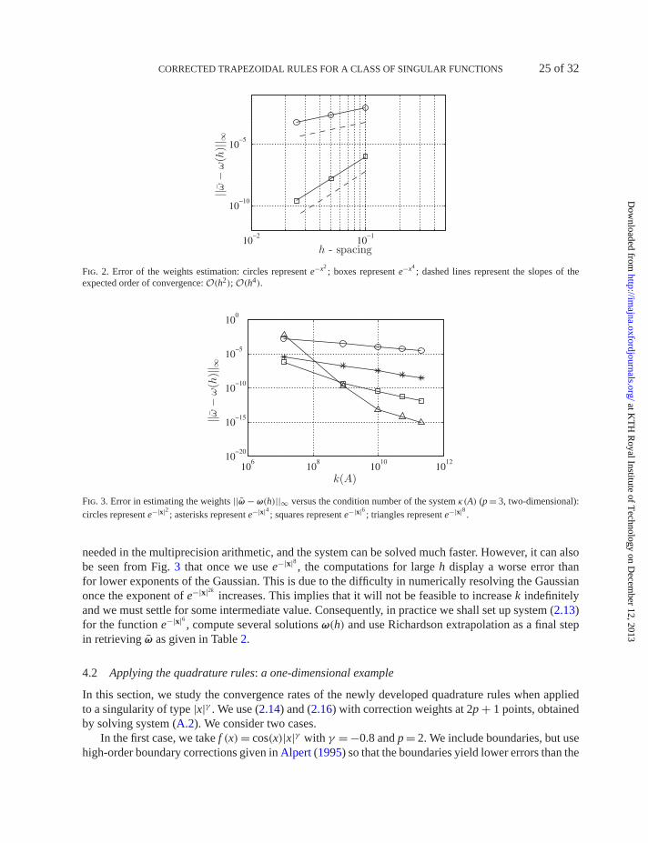
In one dimension the vector of converged weights ω can be obtained as the solution of (A.2), usingthe closed form expression of c(γ ), and we use these to measure the errors in ω(h). In Fig. 2 theconvergence rate of the weights is displayed for g(x)= e−x2

and g(x)= e−x4. In the first case, only the

first derivative vanishes at the origin and therefore by Lemma 3.8 we expect a convergence order O(h2).Similarly, for e−x4

all the derivatives up to third-order evaluate to zero at the origin and thus we expectO(h4) convergence. The numerical tests confirm the expected orders of convergence.

In two dimensions, we do not have a direct way to obtain the converged weights and system (2.13)has to be solved as h → 0. A bottleneck in this procedure is the ill conditioning of the linear system;as the number of modified weights increases the reciprocal condition number of the system reachesepsilon of the machine. The aim is to obtain the value of the weights with double precision. Therefore,the systems are solved in multiple precision arithmetic through straightforward Gaussian eliminationfollowed by repeated Richardson extrapolation.

For g(x)= e−|x|2kthe order of convergence of the weights is O(h2k) and a larger value of k can be

used to speed up the convergence. In Fig. 3, for system (2.13) with p = 3, we show how the choice of kcontrols the convergence of the weights with respect to the condition number of the system, κ(A). Notethat the condition number depends only weakly on the choice of g for a fixed h (the data points corre-sponding to the same h essentially line up along vertical lines). On the horizontal axis we can follow thegrowth of the condition number κ(A), while on the vertical axis we can read the error in approximatingthe weights. To achieve an error ‖ω − ω(h)‖∞ below a prescribed tolerance, the condition number willbe lower for a larger k, and fewer digits will be lost in the calculations. Hence, not as many digits are

at KT

H R


ecember 12, 2013


Dow

nloaded from




Fig. 2. Error of the weights estimation: circles represent e−x2; boxes represent e−x4

; dashed lines represent the slopes of theexpected order of convergence: O(h2); O(h4).

Fig. 3. Error in estimating the weights ||ω − ω(h)||∞ versus the condition number of the system κ(A) (p = 3, two-dimensional):circles represent e−|x|2 ; asterisks represent e−|x|4 ; squares represent e−|x|6 ; triangles represent e−|x|8 .

needed in the multiprecision arithmetic, and the system can be solved much faster. However, it can alsobe seen from Fig. 3 that once we use e−|x|8 , the computations for large h display a worse error thanfor lower exponents of the Gaussian. This is due to the difficulty in numerically resolving the Gaussianonce the exponent of e−|x|2k

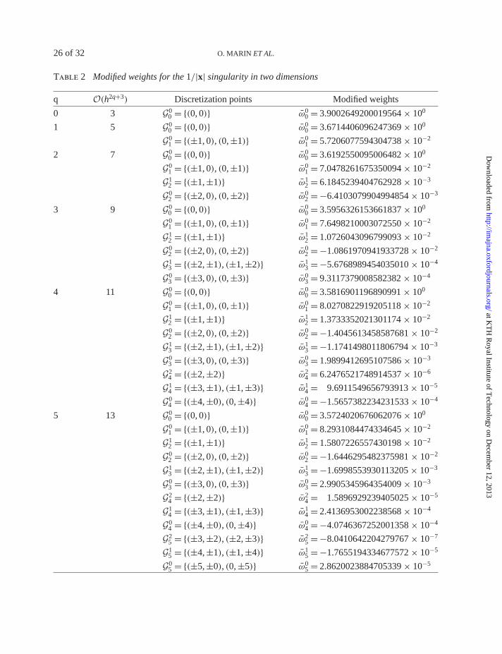
increases. This implies that it will not be feasible to increase k indefinitelyand we must settle for some intermediate value. Consequently, in practice we shall set up system (2.13)for the function e−|x|6 , compute several solutions ω(h) and use Richardson extrapolation as a final stepin retrieving ω as given in Table 2.

4.2 Applying the quadrature rules: a one-dimensional example

In this section, we study the convergence rates of the newly developed quadrature rules when appliedto a singularity of type |x|γ . We use (2.14) and (2.16) with correction weights at 2p + 1 points, obtainedby solving system (A.2). We consider two cases.

In the first case, we take f (x)= cos(x)|x|γ with γ = −0.8 and p = 2. We include boundaries, but usehigh-order boundary corrections given in Alpert (1995) so that the boundaries yield lower errors than the

at KT

H R


ecember 12, 2013


Dow

nloaded from




Table 2 Modified weights for the 1/|x| singularity in two dimensions

q O(h2q+3) Discretization points Modified weights

0 3 G00 = {(0, 0)} ω0

0 = 3.9002649200019564 × 100

1 5 G00 = {(0, 0)} ω0

0 = 3.6714406096247369 × 100

G01 = {(±1, 0), (0, ±1)} ω0

1 = 5.7206077594304738 × 10−2

2 7 G00 = {(0, 0)} ω0

0 = 3.6192550095006482 × 100

G01 = {(±1, 0), (0, ±1)} ω0

1 = 7.0478261675350094 × 10−2

G12 = {(±1, ±1)} ω1

2 = 6.1845239404762928 × 10−3

G02 = {(±2, 0), (0, ±2)} ω0

2 = −6.4103079904994854 × 10−3

3 9 G00 = {(0, 0)} ω0

0 = 3.5956326153661837 × 100

G01 = {(±1, 0), (0, ±1)} ω0

1 = 7.6498210003072550 × 10−2

G12 = {(±1, ±1)} ω1

2 = 1.0726043096799093 × 10−2

G02 = {(±2, 0), (0, ±2)} ω0

2 = −1.0861970941933728 × 10−2

G13 = {(±2, ±1), (±1, ±2)} ω1

3 = −5.6768989454035010 × 10−4

G03 = {(±3, 0), (0, ±3)} ω0

3 = 9.3117379008582382 × 10−4

4 11 G00 = {(0, 0)} ω0

0 = 3.5816901196890991 × 100

G01 = {(±1, 0), (0, ±1)} ω0

1 = 8.0270822919205118 × 10−2

G12 = {(±1, ±1)} ω1

2 = 1.3733352021301174 × 10−2

G02 = {(±2, 0), (0, ±2)} ω0

2 = −1.4045613458587681 × 10−2

G13 = {(±2, ±1), (±1, ±2)} ω1

3 = −1.1741498011806794 × 10−3

G03 = {(±3, 0), (0, ±3)} ω0

3 = 1.9899412695107586 × 10−3

G24 = {(±2, ±2)} ω2

4 = 6.2476521748914537 × 10−6

G14 = {(±3, ±1), (±1, ±3)} ω1

4 = 9.6911549656793913 × 10−5

G04 = {(±4, ±0), (0, ±4)} ω0

4 = −1.5657382234231533 × 10−4

5 13 G00 = {(0, 0)} ω0

0 = 3.5724020676062076 × 100

G01 = {(±1, 0), (0, ±1)} ω0

1 = 8.2931084474334645 × 10−2

G12 = {(±1, ±1)} ω1

2 = 1.5807226557430198 × 10−2

G02 = {(±2, 0), (0, ±2)} ω0

2 = −1.6446295482375981 × 10−2

G13 = {(±2, ±1), (±1, ±2)} ω1

3 = −1.6998553930113205 × 10−3

G03 = {(±3, 0), (0, ±3)} ω0

3 = 2.9905345964354009 × 10−3

G24 = {(±2, ±2)} ω2

4 = 1.5896929239405025 × 10−5

G14 = {(±3, ±1), (±1, ±3)} ω1

4 = 2.4136953002238568 × 10−4

G04 = {(±4, ±0), (0, ±4)} ω0

4 = −4.0746367252001358 × 10−4

G25 = {(±3, ±2), (±2, ±3)} ω2

5 = −8.0410642204279767 × 10−7

G15 = {(±4, ±1), (±1, ±4)} ω1

5 = −1.7655194334677572 × 10−5

G05 = {(±5, ±0), (0, ±5)} ω0

5 = 2.8620023884705339 × 10−5

at KT

H R


ecember 12, 2013


Dow

nloaded from




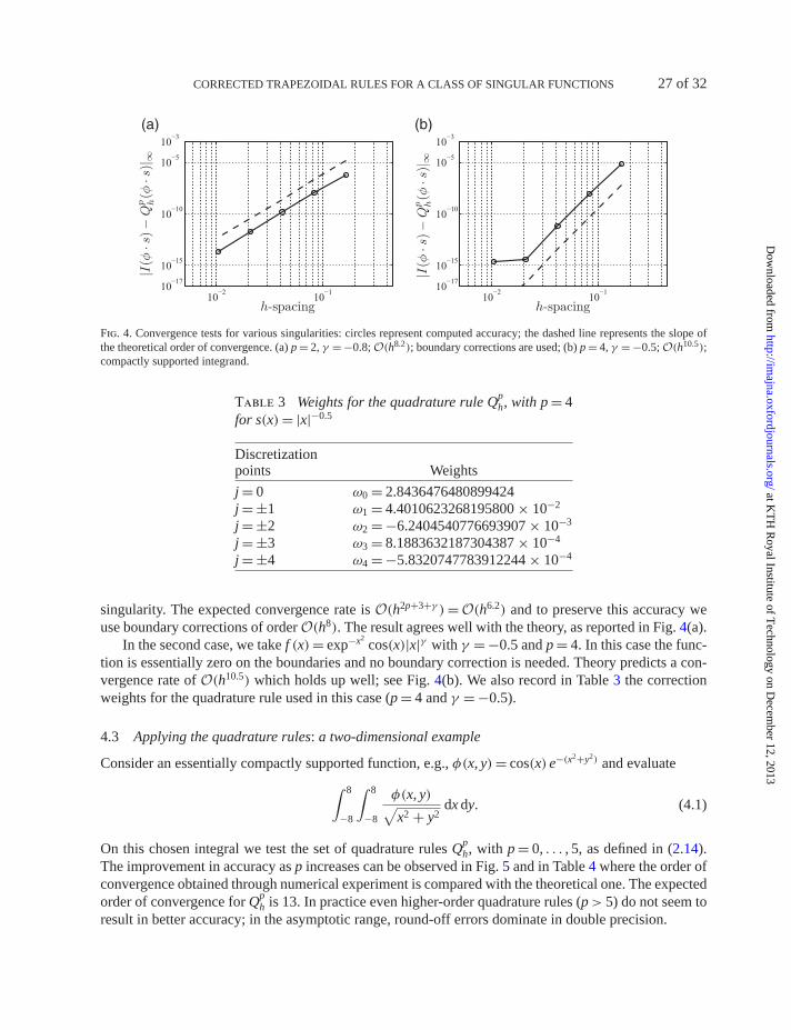
(a) (b)

Fig. 4. Convergence tests for various singularities: circles represent computed accuracy; the dashed line represents the slope ofthe theoretical order of convergence. (a) p = 2, γ = −0.8; O(h8.2); boundary corrections are used; (b) p = 4, γ = −0.5; O(h10.5);compactly supported integrand.

Table 3 Weights for the quadrature rule Qph, with p = 4

for s(x)= |x|−0.5

Discretizationpoints Weights

j = 0 ω0 = 2.8436476480899424j = ±1 ω1 = 4.4010623268195800 × 10−2

j = ±2 ω2 = −6.2404540776693907 × 10−3

j = ±3 ω3 = 8.1883632187304387 × 10−4

j = ±4 ω4 = −5.8320747783912244 × 10−4

singularity. The expected convergence rate is O(h2p+3+γ )=O(h6.2) and to preserve this accuracy weuse boundary corrections of order O(h8). The result agrees well with the theory, as reported in Fig. 4(a).

In the second case, we take f (x)= exp−x2cos(x)|x|γ with γ = −0.5 and p = 4. In this case the func-

tion is essentially zero on the boundaries and no boundary correction is needed. Theory predicts a con-vergence rate of O(h10.5) which holds up well; see Fig. 4(b). We also record in Table 3 the correctionweights for the quadrature rule used in this case (p = 4 and γ = −0.5).

4.3 Applying the quadrature rules: a two-dimensional example

Consider an essentially compactly supported function, e.g., φ(x, y)= cos(x) e−(x2+y2) and evaluate∫ 8

−8

∫ 8

−8

φ(x, y)√x2 + y2

dx dy. (4.1)

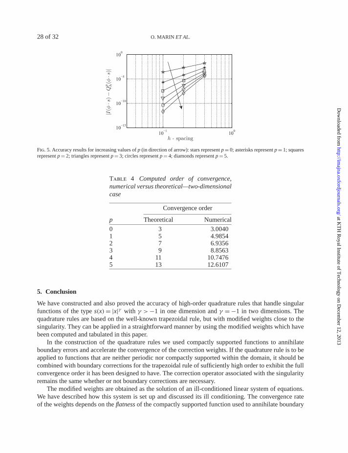
On this chosen integral we test the set of quadrature rules Qph, with p = 0, . . . , 5, as defined in (2.14).

The improvement in accuracy as p increases can be observed in Fig. 5 and in Table 4 where the order ofconvergence obtained through numerical experiment is compared with the theoretical one. The expectedorder of convergence for Qp

h is 13. In practice even higher-order quadrature rules (p> 5) do not seem toresult in better accuracy; in the asymptotic range, round-off errors dominate in double precision.

at KT

H R


ecember 12, 2013


Dow

nloaded from




Fig. 5. Accuracy results for increasing values of p (in direction of arrow): stars represent p = 0; asterisks represent p = 1; squaresrepresent p = 2; triangles represent p = 3; circles represent p = 4; diamonds represent p = 5.

Table 4 Computed order of convergence,numerical versus theoretical—two-dimensionalcase

Convergence order

p Theoretical Numerical

0 3 3.00401 5 4.98542 7 6.93563 9 8.85634 11 10.74765 13 12.6107

5. Conclusion

We have constructed and also proved the accuracy of high-order quadrature rules that handle singularfunctions of the type s(x)= |x|γ with γ >−1 in one dimension and γ = −1 in two dimensions. Thequadrature rules are based on the well-known trapezoidal rule, but with modified weights close to thesingularity. They can be applied in a straightforward manner by using the modified weights which havebeen computed and tabulated in this paper.

In the construction of the quadrature rules we used compactly supported functions to annihilateboundary errors and accelerate the convergence of the correction weights. If the quadrature rule is to beapplied to functions that are neither periodic nor compactly supported within the domain, it should becombined with boundary corrections for the trapezoidal rule of sufficiently high order to exhibit the fullconvergence order it has been designed to have. The correction operator associated with the singularityremains the same whether or not boundary corrections are necessary.

The modified weights are obtained as the solution of an ill-conditioned linear system of equations.We have described how this system is set up and discussed its ill conditioning. The convergence rateof the weights depends on the flatness of the compactly supported function used to annihilate boundary

at KT

H R


ecember 12, 2013


Dow

nloaded from




errors, i.e., on the number of derivatives that vanish at the singular point. We illustrate this propertyin numerical examples and prove mathematically its validity in the one-dimensional case. With animproved convergence rate for the weights, a larger h can be used, which to some extent alleviatesthe ill-conditioning problem. To be able to compute the weights with 16 correct digits, a multiprecisionlibrary is used. In one dimension, we were able to find an analytical expression for the right-hand sideof the system such that converged weights can be computed directly (see the Appendix).

The methodology for setting up the system for the weights can be extended also to other singulari-ties, e.g., the fundamental solution of the Stokes equations (see Marin et al., 2012) which is not radiallysymmetric in all its tensorial components as the functions |x|γ , and more complicated symmetries, mustbe taken into account.

The integration of 1/|x| in R2 as considered here, can also be viewed as an integration of the fun-

damental solution of the Laplace equation over a flat surface in R3. This relates to the discretization of

boundary integral formulations, where integrals are to be evaluated over the boundaries of the domain,be it an outer boundary, the surface of a scattering object in an electromagnetic application or the sur-face of an immersed particle in Stokes flow. We therefore plan to extend this work to also consider theintegration of weakly singular integrals over more general smooth surfaces.

Acknowledgements

The support and enthusiasm with which Hans Riesel has met all our questions on Bernoulli numbersand the Riemann zeta function is gratefully acknowledged.

Funding

References

Abramowitz, M. & Stegun, I. A. (1964) Handbook of Mathematical Functions with Formulas, Graphs, andMathematical Tables, 9th edn. Mineola, NY, USA: Dover Publications.

Aguilar, J. C. & Chen, Y. (2002) High-order corrected trapezoidal quadrature rules for functions with a logarith-mic singularity in 2-D. Comput. Math. Appl., 44, 1031–1039.

Aguilar, J. C. & Chen, Y. (2005) High-order corrected trapezoidal quadrature rules for the Coulomb potential inthree dimensions. Comput. Math. Appl., 49, 625–631.

Alpert, B. K. (1995) High-order quadratures for integral operators with singular kernels. J. Comput. Appl. Math.,60, 367–378.

Alpert, B. K. (1999) Hybrid Gauss-trapezoidal quadrature rules. SIAM J. Sci. Comput., 20, 1551–1584.Atkinson, K. (2004) Quadrature of singular integrands over surfaces. Electron. Trans. Numer. Anal., 17, 133–150.Bruno, O. P. & Kunyansky, L. A. (2001) A fast, high-order algorithm for the solution of surface scattering

problems: basic implementation. J. Comput. Phys., 169, 80–110.Cohen, H. (2007) Number Theory. Vol. II. Analytic and Modern Tools. New York, USA: Springer.Duan, R. & Rokhlin, V. (2009) High-order quadratures for the solution of scattering problems in two dimensions.

J. Comput. Phys., 228, 2152–2174.Duffy, M. G. (1982) Quadrature over a pyramid or cube of integrands with a singularity at a vertex. SIAM J.

Numer. Anal., 19, 1260–1262.Kapur, S. & Rokhlin, V. (1997) High-order corrected trapezoidal quadrature rules for singular functions. SIAM

J. Numer. Anal., 34, 1331–1356.Keast, P. & Lyness, J. N. (1979) On the structure of fully symmetric multidimensional quadrature rules. SIAM J.

Numer. Anal., 16, 11–29.

at KT

H R


ecember 12, 2013


Dow

nloaded from




Khayat, M. A. & Wilton, D. R. (2005) Numerical evaluation of singular and near-singular potential integrals.IEEE Trans. Antennas and Propagation, 53, 3180–3190.

Lyness, J. N. (1976) An error functional expansion for N-dimensional quadrature with an integrand function sin-gular at a point. Math. Comput., 30, 1–23.

Marin, O., Gustavsson, K. & Tornberg, A.-K. (2012) A highly accurate boundary treatment for confined Stokesflow. Comput. & Fluids, 66, 215–230.

Mousavi, S. E. & Sukumar, N. (2010) Generalized Duffy transformation for integrating vertex singularities.Comput. Mech., 45, 127–140.

Pozrikidis, C. (1992) Boundary Integral and Singularity Methods for Linearized Viscous Flow. Cambridge, UK:Cambridge University Press.

Rokhlin, V. (1990) Endpoint corrected trapezoidal quadrature rules for singular functions. Comput. Math. Appl.,20, 51–62.

Sidi, A. (2005) Applications of class Sm variable transformations to numerical integration over surfaces of spheres.J. Comput. Appl. Math., 184, 475–492.

Appendix. Analytical expression for weights (one-dimensional case)

For the one-dimensional case we are able to provide an analytical expression for the weights. Theweights are a solution, as a function of h, of system (2.13) which reads

KI(h)ω(h)= c(h). (A.1)

From Lemma 3.8 we know that I(h) converges to the identity matrix and if we could obtain an analyticalexpression, c(γ ) which is the limit value of the right-hand side, the weights could be computed simplyby solving a system independent of the discretization such as

Kω = c(γ ), (A.2)

where the vector c(γ ) has elements (c0, . . . , cNp−1) with ci = c(γ + 2i). The function c(γ ) was firstencountered in Theorem 3.1 and consequently shown to have the form1

c(γ )=∫ 1

−1s(x)(1 − ψ(x)) dx − 4�

∞∑k=1

W(2πk)

(2πk)2q.

In Lemma A2 we will show that c(γ )= −2ζ(−γ ), where ζ is the Riemann zeta function. In the proofwe will make use of the expansion of ζ(γ ) around the pole at γ = 1.

Theorem A1 (Riemann zeta function) For all integers q � 1 and complex values γ with �γ < 2q,

ζ(−γ )= − 1

γ + 1+ 1

2−

q∑j=1

B2j

(2j)!s(2j−1)(1)− 1

(2q)!

∫ ∞

1s(2q)(x)B2q({x}) dx,

where s(x)= xγ .

1 We use q instead of q + 1 here for notational simplicity.

at KT

H R


ecember 12, 2013


Dow

nloaded from




The result in Theorem A1 can be found, for instance, in Abramowitz & Stegun (1964, Formula23.2.3, p. 807).

Lemma A2 The expression of c(γ ) corresponding to a singularity s(x)= |x|γ which generates the right-hand side to system (A.2) has the closed form expression

c(γ )= −2ζ(−γ ),

where ζ is the Riemann zeta function.

Using definition (3.11) of W(k) we have

4�∞∑

k=1

W(2πk)

(2πk)2q= 4�

∞∑k=1

(2π ik)−2q∫ ∞

0

(d2q

dx2qψ(x)s(x)

)e2π ikx dx

= 2�∞∑

k=1

(2π ik)−2q∫ (

dq

dx2qψ(x)s(x)

)e2π ikx dx

=∫ (

d2q

dx2qψ(x)s(x)

) ∑k |= 0

e2π ikx

(2π ik)2qdx

= − 1

(2q)!

∫ (d2q

dx2qψ(x)s(x)

)B2q({x}) dx,

where we used the formula for the Fourier series of Bq(x), 0 � x< 1. Thus,

c(γ )=∫ 1

−1s(x)(1 − ψ(x)) dx + 1

(2q)!

∫ (d2q

dx2qψ(x)s(x)

)B2q({x}) dx.

Since B2q(1 − x)= B2q(x) then by the symmetry of all functions,

1

2c(γ )=

∫ 1

0s(x)(1 − ψ(x)) dx + 1

(2q)!

∫ ∞

0

(d2q

dx2qψ(x)s(x)

)B2q({x}) dx. (A.3)

To evaluate the last integral in (A.3), we will now use the Euler–Maclaurin (Theorem 1.1) summationformula for the integral over [0, 1] and Theorem A1 for the rest. We also need the fact that sinceψ(x)≡ 1for x � 1,

dj

dxjψ(x)s(x)

∣∣∣∣x=1

= s(j)(1), j � 0.

at KT

H R


ecember 12, 2013


Dow

nloaded from




We get

1

(2q)!

∫ ∞

0

(d2q

dx2qψ(x)s(x)

)B2q({x}) dx = 1

(2q)!

∫ 1

0

(d2q

dx2qψ(x)s(x)

)B2q({x}) dx

+ 1

(2q)!

∫ ∞

1s(2q)(x)B2q({x}) dx

=∫ 1

0ψ(x)s(x) dx − 1

2s(1)+

q∑j=1

B2j

(2j)!s(2j−1)(1)

− ζ(−γ )− 1

γ + 1+ 1

2−

q∑j=1

B2j

(2j)!s(2j−1)(1)

=∫ 1

0ψ(x)s(x) dx − ζ(−γ )−

∫ 1

0s(x) dx.

Together with (A.3), this shows thatc(γ )= −2ζ(−γ ). (A.4)

at KT

H R


ecember 12, 2013


Dow

nloaded from



Corrected trapezoidal rules for a class of singular …olofr/Publications/gentrap.pdf · Corrected trapezoidal rules for a class of singular ... and Chen designed singularity-corrected

Documents