Copyright © Cengage Learning. All rights reserved. 8 Further Applications of Integration

Copyright © Cengage Learning. All rights reserved. 8 Further Applications of Integration.
Dec 19, 2015
Welcome message from author
This document is posted to help you gain knowledge. Please leave a comment to let me know what you think about it! Share it to your friends and learn new things together.
Transcript

Copyright © Cengage Learning. All rights reserved.
8Further Applications
of Integration

Copyright © Cengage Learning. All rights reserved.
8.4 Applications to Economics and Biology

33
Applications to Economics and Biology
In this section we consider some applications of integration
to economics (consumer surplus) and biology (blood flow,
cardiac output).
44
Consumer Surplus

55
Consumer Surplus
Recall that the demand function p(x) is the price that a company has to charge in order to sell x units of a commodity.
Usually, selling larger quantities
requires lowering prices, so the
demand function is a decreasing
function. The graph of a typical
demand function, called a
demand curve, is shown in Figure 1.
If X is the amount of the commodity that
is currently available, then P = p(X) is
the current selling price.
Figure 1
A typical demand curve
66
Consumer Surplus
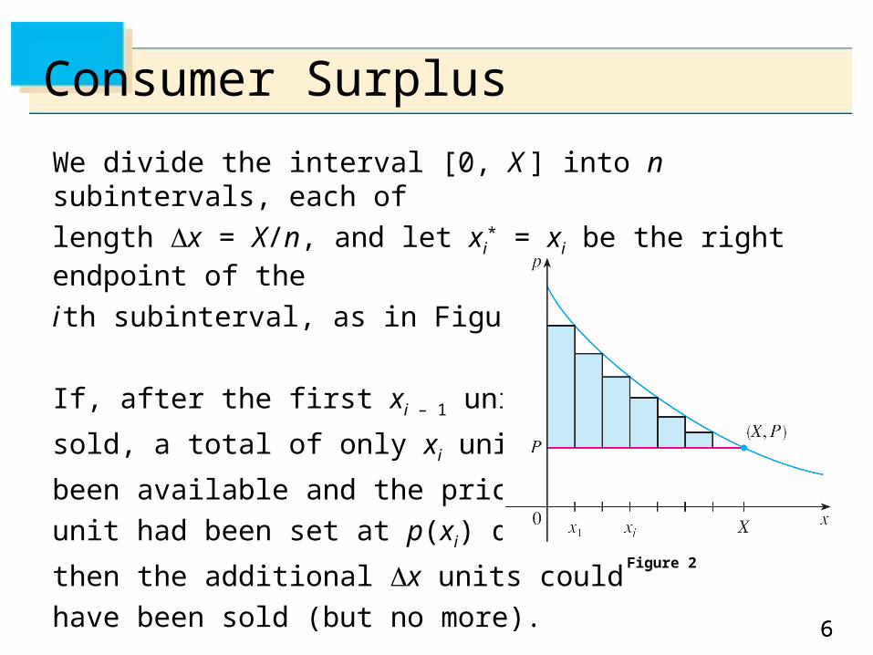
We divide the interval [0, X ] into n subintervals, each of
length x = X/n, and let xi* = xi be the right endpoint of the
i th subinterval, as in Figure 2.
If, after the first xi – 1 units were
sold, a total of only xi units had
been available and the price per
unit had been set at p(xi) dollars,
then the additional x units could
have been sold (but no more). Figure 2
77
Consumer Surplus
The consumers who would have paid p(xi) dollars placed a high value on the product; they would have paid what it was worth to them.
So, in paying only P dollars they have saved an amount of
(savings per unit) (number of units) = [p(xi) – P] x
88
Consumer Surplus
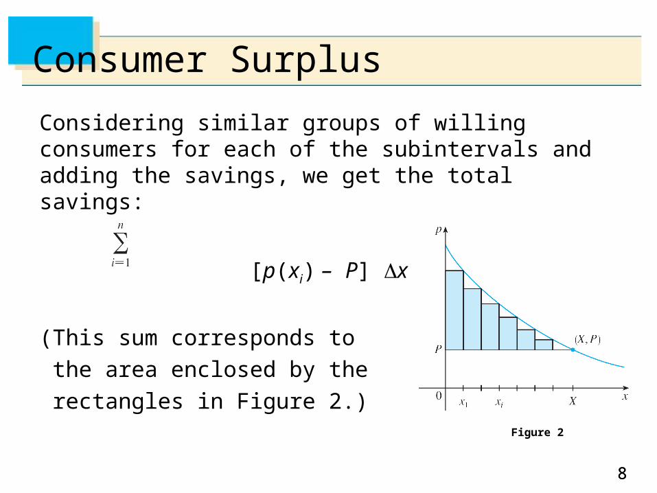
Considering similar groups of willing consumers for each of the subintervals and adding the savings, we get the total savings:
[p(xi) – P] x
(This sum corresponds to
the area enclosed by the
rectangles in Figure 2.)
Figure 2
99
Consumer Surplus
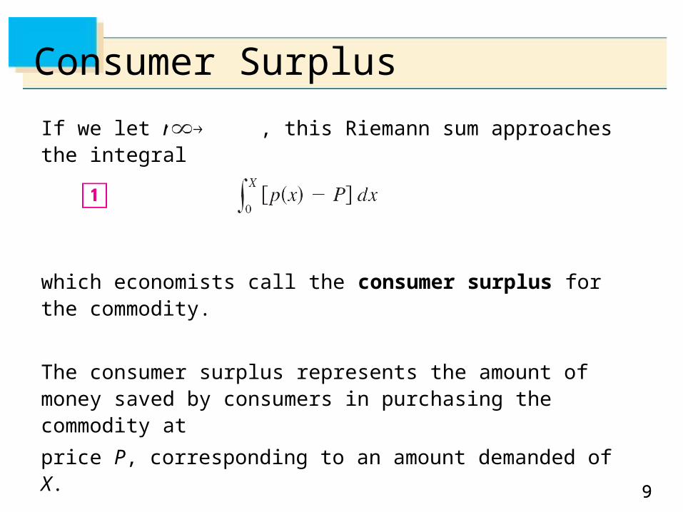
If we let n , this Riemann sum approaches the integral
which economists call the consumer surplus for the commodity.
The consumer surplus represents the amount of money saved by consumers in purchasing the commodity at
price P, corresponding to an amount demanded of X.

1010
Consumer Surplus
Figure 3 shows the interpretation of the consumer surplus
as the area under the demand curve and above the line
p = P.
Figure 3

1111
Example 1
The demand for a product, in dollars, is
p = 1200 – 0.2x – 0.0001x2
Find the consumer surplus when the sales level is 500.
Solution:
Since the number of products sold is X = 500, the corresponding price is
P = 1200 – (0.2)(500) – (0.0001)(500)2
= 1075
1212
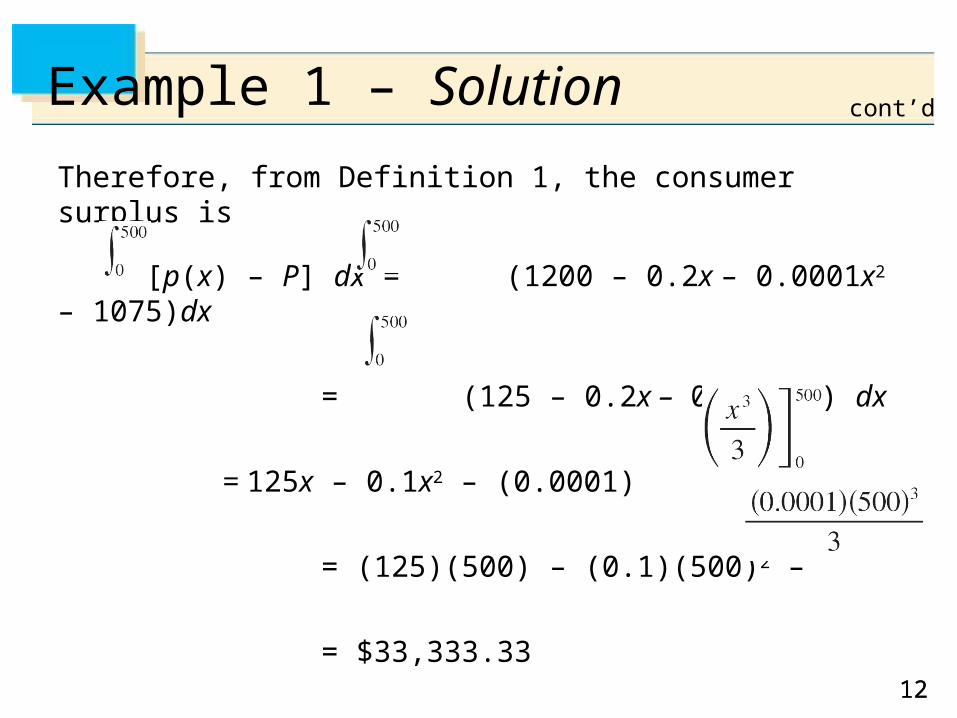
Therefore, from Definition 1, the consumer surplus is
[p(x) – P] dx = (1200 – 0.2x – 0.0001x2 – 1075)dx
= (125 – 0.2x – 0.0001x2) dx
= 125x – 0.1x2 – (0.0001)
= (125)(500) – (0.1)(500)2 –
= $33,333.33
Example 1 – Solution cont’d
1313
Blood Flow
1414
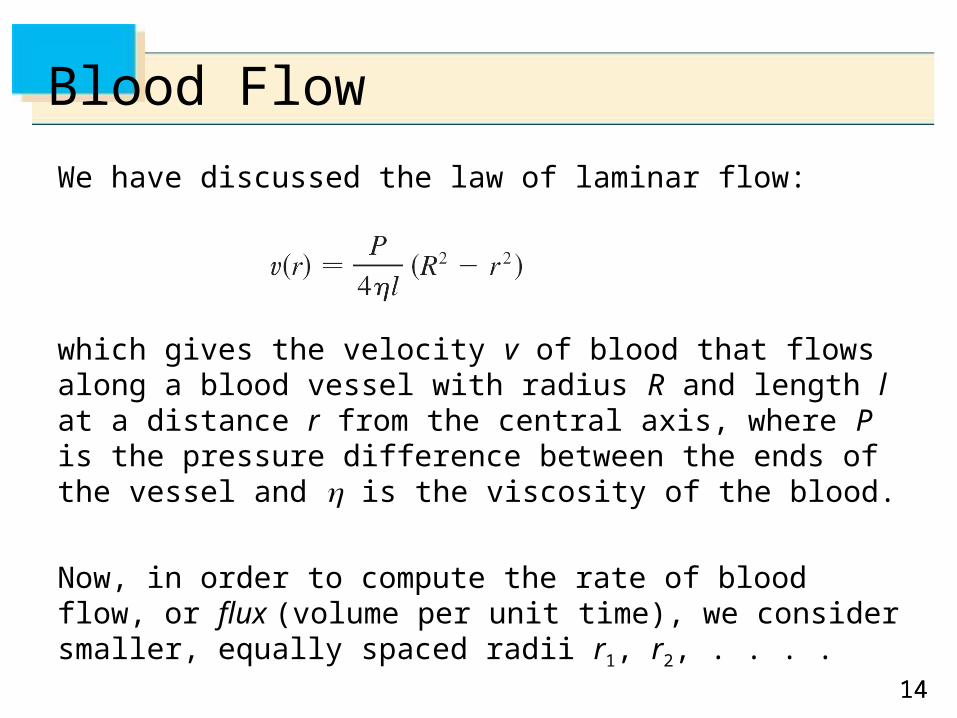
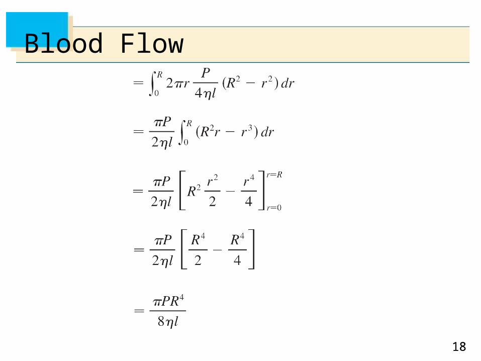
We have discussed the law of laminar flow:
which gives the velocity v of blood that flows along a blood vessel with radius R and length l at a distance r from the central axis, where P is the pressure difference between the ends of the vessel and is the viscosity of the blood.
Now, in order to compute the rate of blood flow, or flux (volume per unit time), we consider smaller, equally spaced radii r1, r2, . . . .
Blood Flow
1515
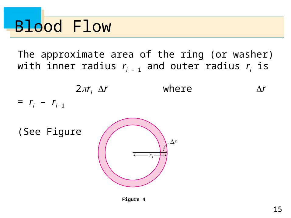
The approximate area of the ring (or washer) with inner radius ri – 1 and outer radius ri is
2ri r where r = ri – ri –1
(See Figure 4.)
Blood Flow
Figure 4
1616
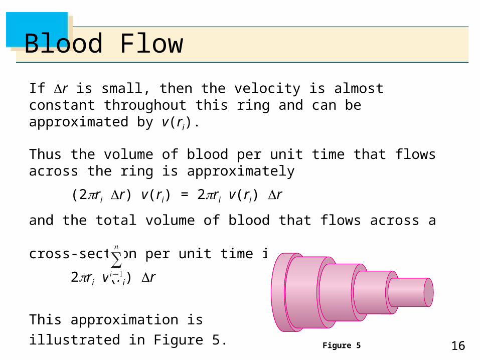
If r is small, then the velocity is almost constant throughout this ring and can be approximated by v(ri).
Thus the volume of blood per unit time that flows across the ring is approximately
(2ri r) v(ri) = 2ri v(ri) r
and the total volume of blood that flows across a cross-section per unit time is about
2ri v(ri) r
This approximation is
illustrated in Figure 5.
Blood Flow
Figure 5
1717
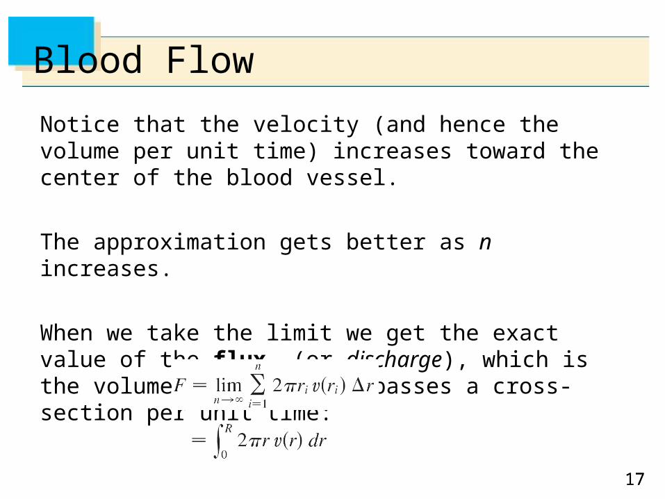
Notice that the velocity (and hence the volume per unit time) increases toward the center of the blood vessel.
The approximation gets better as n increases.
When we take the limit we get the exact value of the flux (or discharge), which is the volume of blood that passes a cross-section per unit time:
Blood Flow
1818
Blood Flow
1919
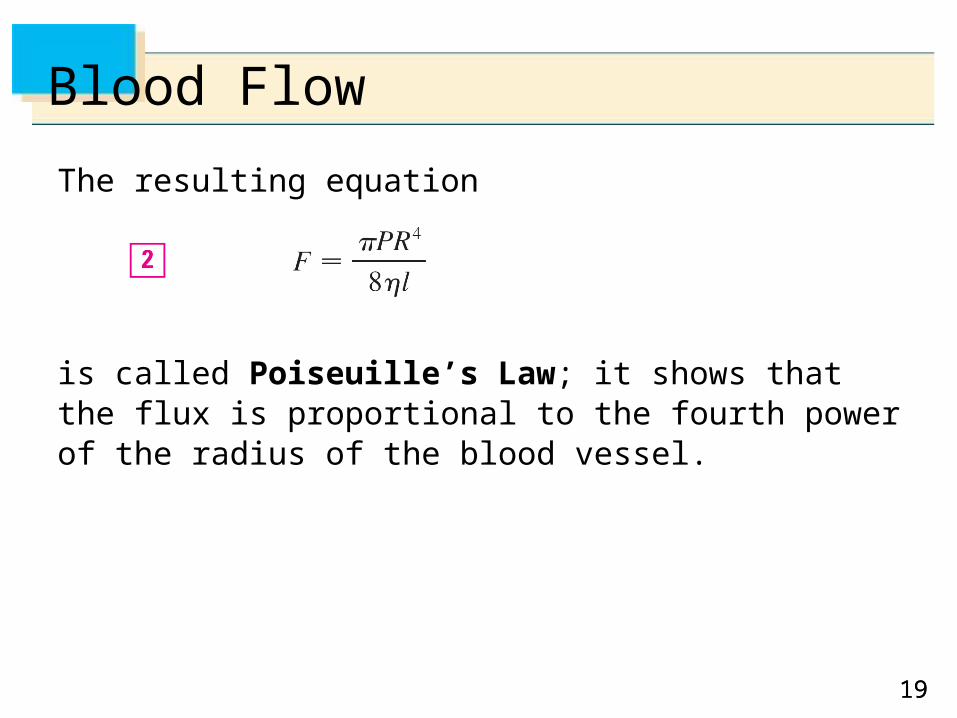
The resulting equation
is called Poiseuille’s Law; it shows that the flux is proportional to the fourth power of the radius of the blood vessel.
Blood Flow
2020
Cardiac Output
2121
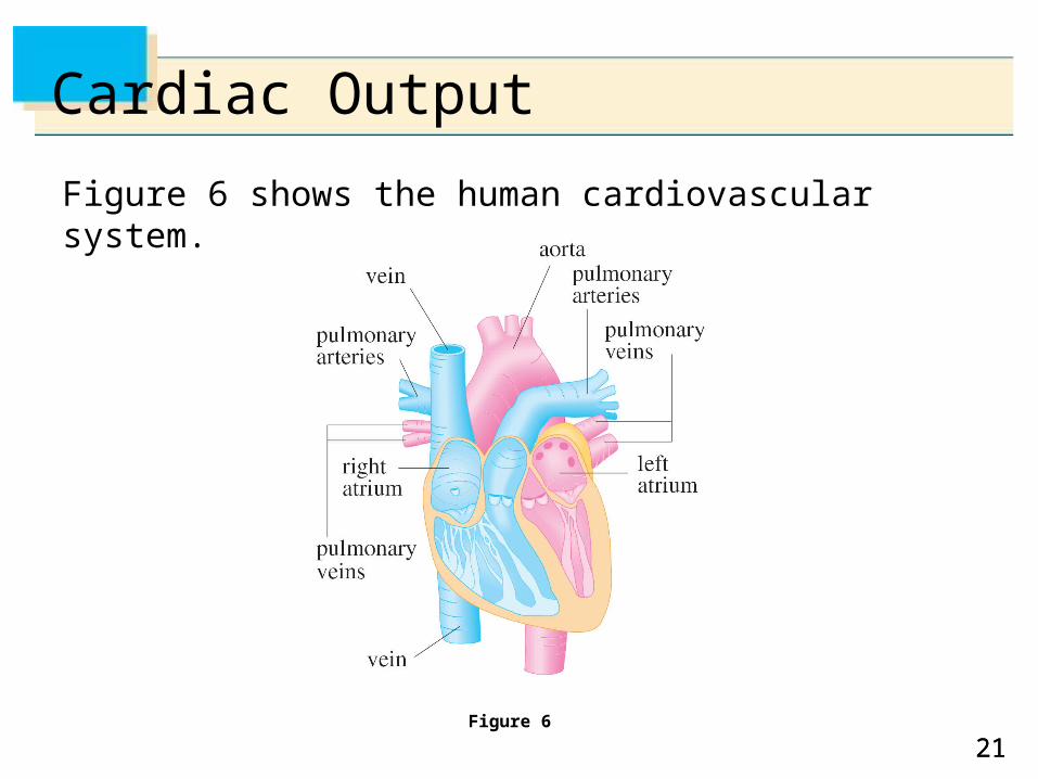
Figure 6 shows the human cardiovascular system.
Cardiac Output
Figure 6
2222
Blood returns from the body through the veins, enters the right atrium of the heart, and is pumped to the lungs through the pulmonary arteries for oxygenation.
It then flows back into the left atrium through the pulmonary veins and then out to the rest of the body through the aorta.
The cardiac output of the heart is the volume of blood pumped by the heart per unit time, that is, the rate of flow into the aorta.
The dye dilution method is used to measure the cardiac output.
Cardiac Output
2323
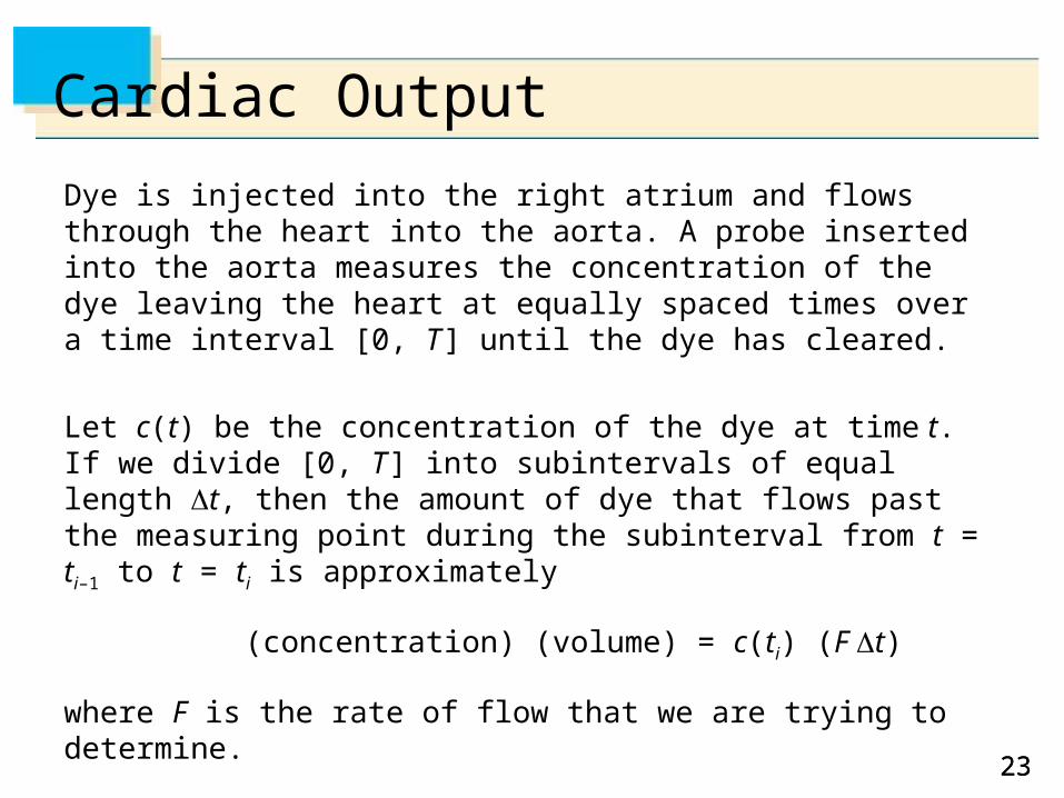
Dye is injected into the right atrium and flows through the heart into the aorta. A probe inserted into the aorta measures the concentration of the dye leaving the heart at equally spaced times over a time interval [0, T ] until the dye has cleared.
Let c(t) be the concentration of the dye at time t. If we divide [0, T ] into subintervals of equal length t, then the amount of dye that flows past the measuring point during the subinterval from t = ti–1 to t = ti is approximately
(concentration) (volume) = c(ti) (F t)
where F is the rate of flow that we are trying to determine.
Cardiac Output
2424
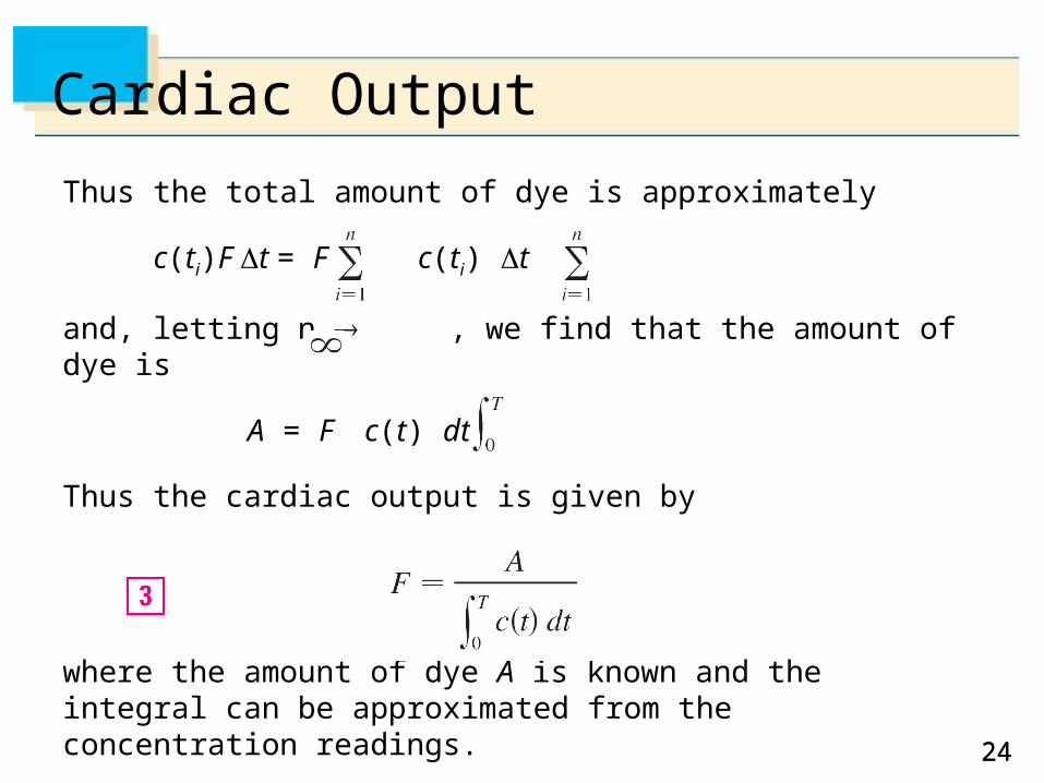
Thus the total amount of dye is approximately
c(ti)F t = F c(ti) t
and, letting n , we find that the amount of dye is
A = F c(t) dt
Thus the cardiac output is given by
where the amount of dye A is known and the integral can be approximated from the concentration readings.
Cardiac Output
2525
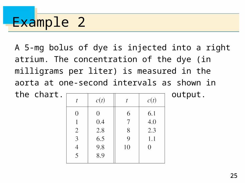
Example 2
A 5-mg bolus of dye is injected into a right atrium. The
concentration of the dye (in milligrams per liter) is
measured in the aorta at one-second intervals as shown in
the chart. Estimate the cardiac output.

2626
Example 2 – Solution
Here A = 5, t = 1, and T = 10. We use Simpson’s Rule to approximate the integral of the concentration:
c(t) dt [0 + 4(0.4) + 2(2.8) + 4(6.5) + 2(9.8) + 4(8.9)
+ 2(6.1) + 4(4.0) + 2(2.3) + 4(1.1) + 0]
41.87
Thus Formula 3 gives the cardiac output to be
0.12 L/s
= 7.2 L/min
Related Documents