Degree project in Controller-Inverter for Sensorless Permanent Magnet Synchronous Motors Application in Onboard Electric Powertrain for Uphill Propulsion in Downhill Mountain Biking MATTIAS RAHM Stockholm, Sweden 2012 XR-EE-E2C 2012:006 Electrical Engineering Master of Science

Welcome message from author
This document is posted to help you gain knowledge. Please leave a comment to let me know what you think about it! Share it to your friends and learn new things together.
Transcript
Degree project in
Controller-Inverter for SensorlessPermanent Magnet Synchronous Motors
Application in Onboard Electric Powertrain for Uphill Propulsion in Downhill Mountain Biking
MATTIAS RAHM
Stockholm, Sweden 2012
XR-EE-E2C 2012:006
Electrical EngineeringMaster of Science
Controller-Inverter for Sensorless Permanent Magnet Synchronous Motors
Application in Onboard Electric Powertrain for Uphill Propulsion in Downhill Mountain Biking
by
Mattias Rahm
Master Thesis
Royal Institute of Technology School of Electrical Engineering
Electrical Energy Conversion
Stockholm 2012 XR-EE-E2C 2012:006

iii
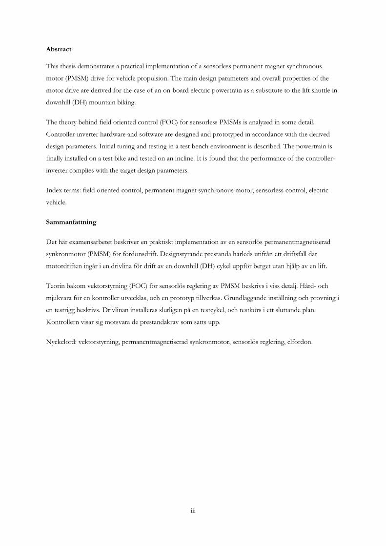
Abstract
This thesis demonstrates a practical implementation of a sensorless permanent magnet synchronous
motor (PMSM) drive for vehicle propulsion. The main design parameters and overall properties of the
motor drive are derived for the case of an on-board electric powertrain as a substitute to the lift shuttle in
downhill (DH) mountain biking.
The theory behind field oriented control (FOC) for sensorless PMSMs is analyzed in some detail.
Controller-inverter hardware and software are designed and prototyped in accordance with the derived
design parameters. Initial tuning and testing in a test bench environment is described. The powertrain is
finally installed on a test bike and tested on an incline. It is found that the performance of the controller-
inverter complies with the target design parameters.
Index terms: field oriented control, permanent magnet synchronous motor, sensorless control, electric
vehicle.
Sammanfattning
Det här examensarbetet beskriver en praktiskt implementation av en sensorlös permanentmagnetiserad
synkronmotor (PMSM) för fordonsdrift. Designstyrande prestanda härleds utifrån ett driftsfall där
motordriften ingår i en drivlina för drift av en downhill (DH) cykel uppför berget utan hjälp av en lift.
Teorin bakom vektorstyrning (FOC) för sensorlös reglering av PMSM beskrivs i viss detalj. Hård- och
mjukvara för en kontroller utvecklas, och en prototyp tillverkas. Grundläggande inställning och provning i
en testrigg beskrivs. Drivlinan installeras slutligen på en testcykel, och testkörs i ett sluttande plan.
Kontrollern visar sig motsvara de prestandakrav som satts upp.
Nyckelord: vektorstyrning, permanentmagnetiserad synkronmotor, sensorlös reglering, elfordon.


v
Acknowledgements
A debt of gratitude is owed to several people, and most notably to
- Professor Hans-Peter Nee at KTH for accepting the supervision of this thesis.
- Associate professor Oskar Wallmark at KTH for sharing your expertise on the control of the
PMSM.
- Stefan Skär and Imre Sjöberg at ABB Substations for letting me take the time off needed to
pursue my master's studies, despite the occasional consequences.
- Mattias Bäck at Conrit for making valuable machine time available at student pricing.
- The good people at Micro-Kit Elektronik for the motor winding measurements, the SMD-
soldering crash course and more.
- William Sandqvist at KTH just for doing your job of providing a terrific introductory course to
embedded programming.
- Daniel Rahm for test riding like I would have never dared; Jonas Man and Oscar Man for
measuring the test slopes with survey-like precision.
And to Sven Samuelsson for your encouraging interest and support; and for preaching what eventually
became the motto for the project: Add Only Lightness1.
Mattias Rahm, Västerås, May 2012
1 A variant of Colin Chapman's (founder of Lotus Cars) quote "Simplify, then add lightness."

vii
Table of Contents
LIST OF ACRONYMS ................................................................................................................................... 1
LIST OF SYMBOLS ....................................................................................................................................... 2
1 INTRODUCTION ................................................................................................................................. 3
1.1 OBJECTIVES .................................................................................................................................................................... 3
1.2 METHOD ......................................................................................................................................................................... 4
1.2.1 Low power and full power experimental setups .............................................................................................................. 4
1.2.2 Procedure and outline of the thesis .................................................................................................................................. 4
2 OVERALL PROPERTIES OF THE MOTOR DRIVE ........................................................................ 5
2.1 SELECTION OF SENSORLESS CONTROL ALGORITHM ............................................................................................... 5
2.1.1 Inverter switching scheme ............................................................................................................................................... 6
2.2 MATCH BETWEEN THE MOTOR AND THE LOAD ...................................................................................................... 7
2.2.1 Choice of gearing ............................................................................................................................................................ 7
2.2.2 Choice of motor ............................................................................................................................................................. 8
2.3 THERMAL CONSIDERATIONS IN SELECTING THE MOTOR .................................................................................... 11
2.4 MATCH BETWEEN THE MOTOR AND THE POWER ELECTRONIC CONVERTER .................................................. 11
2.4.1 Current rating ............................................................................................................................................................. 11
2.4.2 Voltage rating ............................................................................................................................................................. 11
2.4.3 Switching frequency and motor inductance .................................................................................................................... 12
2.5 CURRENT LIMITING..................................................................................................................................................... 12
3 CONTROL OF THE PMSM ................................................................................................................ 13
3.1 FOC – MIMICKING THE DC-MOTOR ....................................................................................................................... 13
3.1.1 A two-phase rotor reference frame model of the PMSM ............................................................................................... 14
3.1.2 The PLL-type estimator .............................................................................................................................................. 16
3.1.3 Field-weakening .......................................................................................................................................................... 19
3.2 DESIGN OF THE CURRENT CONTROLLER ................................................................................................................ 19
3.2.1 PI-tuning by simulation ............................................................................................................................................... 20
3.2.2 The control strategy ...................................................................................................................................................... 23
3.2.3 Torque demand step test with a fan-type load ............................................................................................................... 26
4 PROTOTYPING .................................................................................................................................. 29
4.1 THREE DIMENSIONAL PRINTED CIRCUIT BOARD, HEATSINK AND ENCLOSURE DESIGN ............................... 29
4.2 GROUND BOUNCE ....................................................................................................................................................... 30
4.2.1 Ground bounce mitigation ........................................................................................................................................... 33
4.2.2 Bulk filter capacitance ................................................................................................................................................. 34
5 RESULTS AND CONCLUSION......................................................................................................... 35
5.1 RESULTS ........................................................................................................................................................................ 35
5.1.1 Maximum no-load motor speed ................................................................................................................................... 35
5.1.2 Power factor at nominal load ....................................................................................................................................... 35
5.1.3 Hill climbing capability ............................................................................................................................................... 35
5.1.4 Examination Hill ...................................................................................................................................................... 37
5.1.5 Heat sink and motor temperature rise ......................................................................................................................... 38
5.1.6 Added mass of the motor drive .................................................................................................................................... 38
5.1.7 The inherent start-up problem of the sensorless drive .................................................................................................... 39
5.2 CONCLUSION ................................................................................................................................................................ 40
5.3 AREAS OF FUTURE WORK ........................................................................................................................................... 40
5.3.1 Potential benefits of increased rotor speed...................................................................................................................... 40
5.3.2 Field weakening in SMPMs ....................................................................................................................................... 40
5.3.3 Tailor-made motors ..................................................................................................................................................... 40
viii
5.3.4 Reliable start-up algorithm for heavy loads .................................................................................................................. 41
5.3.5 Capture transient events on trigger ............................................................................................................................... 41
6 REFERENCES .................................................................................................................................... 43
7 APPENDICES ...................................................................................................................................... 45
7.1 APPENDIX A: DERIVATION OF MAIN DESIGN PARAMETERS ............................................................................... 45
7.1.1 Introduction ................................................................................................................................................................. 45
7.1.2 Calculation of input parameters ................................................................................................................................... 46
7.1.3 Rectilinear motion power and torque requirements ........................................................................................................ 46
7.1.4 Single load cycle equivalent battery mass requirement ................................................................................................... 47
7.2 APPENDIX B: EXPERIMENTAL SETUP AND TEST BIKE .......................................................................................... 49
7.2.1 Experimental setup ..................................................................................................................................................... 49
7.2.2 Test bike ..................................................................................................................................................................... 51
7.3 APPENDIX C: PER UNIT MODEL................................................................................................................................ 55
1
List of acronyms
back emf back electromotive force
CMOS complementary metal oxide semiconductor
DH downhill biking
DSP digital signal processor
FOC field oriented control
LiPo lithium polymer
MIPS million instructions per second
PCB printed circuit board
PLL phase lock loop
PMSM permanent magnet synchronous motor
PWM pulse width modulation
R/C radio controlled
rps revolutions per second
SMD surface mount device
SMPM surface mounted permanent magnet synchronous motor
SVM space vector modulation
VSI voltage source inverter

2
List of symbols
^ estimation
˙ [dot above] derivation with respect to time
BL load frictional damping
Bm motor frictional damping
bold vector notation
d derivating operator
e back emf
ids stator d-axis current
iqs stator q-axis current
Is stator average current
JL load inertia
Jm motor inertia
Kt motor torque constant
Kv motor velocity constant
Ls stator inductance
ngear gear ratio
NL number of load gear teeth
Nm number of motor gear teeth
p instantaneous power
Rs stator resistance
Tem electromagnetic torque
VDC-link DC-supply (battery) voltage
vds stator d-axis voltage
vqs stator q-axis voltage
Vs stator voltage vector
θ rotor angle relative to the stator reference frame
λaf rotor magnet flux linkage
ωL load angle velocity
ωm motor mechanical angle velocity
ωr rotor electrical angle velocity
3
1 Introduction
Downhill (DH) mountain biking is quickly becoming a popular summer time activity in alpine resorts and
elsewhere. Lift shuttles are used to reposition the bike and rider on top of the hill. Lately, some
manufacturers are offering electrically assisted DH bikes as a means to augment rideable territory beyond
the shuttle assisted slopes. The KTM eGNITION and the EGO-Kit are some examples. In this way, any
hill becomes a possible DH venue. The combination of the harsh operating conditions found in DH
mountain biking - bumpy, muddy, wet and environmentally constrained - and the border-line anorectic
focus on component weight in the bicycle community makes it an interesting case study for the
application of high power density electric motor drives.
Motors, batteries and controllers from the realm of large radio controlled (R/C) electrical model airplanes
have power ratings on par with the demands of such a drive and are readily available as off-the-shelf
components. Being perhaps the most power dense powertrain components available, they are also well in
compliance with the weight ranges imposed by the example products mentioned above, and are the
natural first choice for a lightweight high-performance motor drive in the sub 10kW power range.
The direct application of an R/C airplane drive on a road vehicle is however problematic. The propeller
load has a fan-like power variation property described by
( ) 1-1
The low start-up torque requirement makes the R/C airplane drive easy to start. At high motor speeds, the
high power demand will counteract any rapid changes in speed. Combined, this makes the fan load an
ideal candidate for the low-cost high-reliability sensorless type drive. This is why all R/C model airplane
motors are manufactured without position sensors, which severely limits the range of controllers available
to run the motor, as most of them tend to rely on external circuitry for rotor positioning. Also, as a
consequence of the low power (and hence low duty cycle) requirements at low speeds, the sensorless R/C
model airplane controller-inverter ratings are valid for high motor speed, high duty cycles only. When used
with loads having characteristics differing from the fan – e.g. a road vehicle – they have a strong tendency
to overheat and fail2.
The native R/C airplane controller-inverter is hence useless for mountain duty, and a more robust
alternative is not commercially available. In order to take advantage of the power density of model
airplane motors and batteries, a suitable controller is missing. Such a controller is the focus of this thesis.
1.1 Objectives
The purpose of this paper is to derive, design, prototype and verify the main design parameters of a
controller-inverter capable of driving a sensorless R/C-motor based powertrain installed on a DH
mountain bike. As will be demonstrated in later chapters, the R/C motor falls into the permanent magnet
synchronous motor (PMSM) category of motors, which - ideally - implies the implementation of a
sensorless field oriented control (FOC) algorithm.
2 See, for example, the Internet forum Endless-Sphere for abundant anecdotal reference.

4
1.2 Method
The electrical motor drive contains elements from electronics, electric power and electromechanical
engineering, including an energy conversion from electric to rotational power. All of these have to play
well together in order for the motor drive to function properly. The control part - electronics - mediates
the transistors – power electronics – to portion the right amount of electric current at the right time to the
motor windings – the electrical machine. One consequence of this complexity is that a seemingly
unimportant error in the electronics may cause severe damage if the error results in that one or more
power transistors are left in their on-state for too long, thus causing a short-circuit like situation.
Therefore, the method used here is to begin with a failure friendly low power setup, and then – once
functioning properly - to move on to the more powerful final controller-inverter setup.
The purpose of the low power setup is to verify that
- Software is working as expected
- The general approach is valid (PI-control tuning, gate resistor order of magnitude, choice of
processor speed, hardware and software filters etc.)
- Perform speed and load step tests to generate an overall understanding of the drive
The characteristics of the full power setup can then be interpolated from the low power setup results.
Whereas this transition may not be seamless, at least the major question marks should have been resolved
in the low power setup.
1.2.1 Low power and full power experimental setups
The low power development environment is presented in Appendix B: Experimental setup and test bike.
The full power setup is the actual controller-inverter that goes on the bike, and is treated in chapter 4.
1.2.2 Procedure and outline of the thesis
Starting from the power and speed requirements derived in the appendix, the target ratings of the
controller are decided. These ratings are further processed in conjunction with the R/C motor and the
load characteristics in order to decide the general properties of the powertrain. Examples of such
properties are gearing, control algorithm and size of motor. This is done in chapter 2. Chapter 3 focuses
on the actual control algorithm; the theoretical background, the limitations, as well as assumptions and
performance estimations. Tests of the algorithm are done on the low power development setup. Finally, in
chapter 4, the full power controller-inverter design is modeled in 3D CAD software, transferred to PCB
design software and prototyped. The concluding chapter presents the results obtained with the test bike,
and the conclusions drawn.
5
2 Overall properties of the motor drive
In this chapter, the various design consideration that come up in the controller-inverter design process are
described, as well as the design strategies adopted. In [1], a set of criteria for selecting motor drive
components is presented as
- Selection of speed and position sensors3
- Match between the motor and the load
- Thermal considerations in selecting the motor
- Match between the motor and the power electronic converter
o Current rating
o Voltage rating
o Switching frequency and motor inductance
- Current limiting
The reasoning in this chapter largely follows [1], with some excursions.
The scope of this thesis is the power electronic converter. Therefore, considerations concerning the
motor, batteries, gear box, bearing heating, mechanical rpm limitations etc. are presented for reference
only.
2.1 Selection of sensorless control algorithm
The R/C motor type considered in this thesis is not equipped with any sensors to determine the rotor
speed and position. While this may seem as a disadvantage from a control perspective, there are also a
number of advantages. These are well known and include lower hardware cost, less wiring, higher
reliability (fewer components that can fail), less space requirement and the avoidance of sensor mounting
inaccuracies. The selection of a suitable sensorless control algorithm for the motor type at hand is
discussed in the following.
In terms of back emf and line currents, the instantaneous electromagnetic torque produced in a PM
brushless motor is described by
2-1
To minimize ripple in the torque production, the back emf and current waveforms should be as similar as
possible (and of the same phase). When the shapes are equal, the current harmonics are of the same order,
and a constant torque is produced. When the shapes differ, current harmonics of different order interact
to produce a pulsating torque of frequencies being a multiple of the fundamental frequency. Pulsating
torques are the cause of heat generation, vibrations and acoustic noise, and thus highly undesirable. [2]
Brushless PM motors are usually categorized as sinusoidal4 or trapezoidal5 depending on the shape of the
back emf. One of the motors in this study (they are all of the same type and construction) was put in a test
3 A sensorless drive is considered here, and this entry translates into ‘Selection of sensorless control algorithm’.
4 PMSM, PMAC and similar abbreviations are used for this category
6
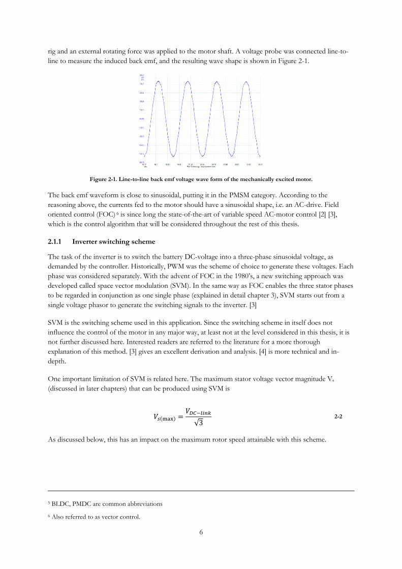
rig and an external rotating force was applied to the motor shaft. A voltage probe was connected line-to-
line to measure the induced back emf, and the resulting wave shape is shown in Figure 2-1.
Figure 2-1. Line-to-line back emf voltage wave form of the mechanically excited motor.
The back emf waveform is close to sinusoidal, putting it in the PMSM category. According to the
reasoning above, the currents fed to the motor should have a sinusoidal shape, i.e. an AC-drive. Field
oriented control (FOC) 6 is since long the state-of-the-art of variable speed AC-motor control [2] [3],
which is the control algorithm that will be considered throughout the rest of this thesis.
2.1.1 Inverter switching scheme
The task of the inverter is to switch the battery DC-voltage into a three-phase sinusoidal voltage, as
demanded by the controller. Historically, PWM was the scheme of choice to generate these voltages. Each
phase was considered separately. With the advent of FOC in the 1980’s, a new switching approach was
developed called space vector modulation (SVM). In the same way as FOC enables the three stator phases
to be regarded in conjunction as one single phase (explained in detail chapter 3), SVM starts out from a
single voltage phasor to generate the switching signals to the inverter. [3]
SVM is the switching scheme used in this application. Since the switching scheme in itself does not
influence the control of the motor in any major way, at least not at the level considered in this thesis, it is
not further discussed here. Interested readers are referred to the literature for a more thorough
explanation of this method. [3] gives an excellent derivation and analysis. [4] is more technical and in-
depth.
One important limitation of SVM is related here. The maximum stator voltage vector magnitude Vs
(discussed in later chapters) that can be produced using SVM is
( )
√ 2-2
As discussed below, this has an impact on the maximum rotor speed attainable with this scheme.
5 BLDC, PMDC are common abbreviations
6 Also referred to as vector control.
7
2.2 Match between the motor and the load
2.2.1 Choice of gearing
In this application, the optimal gearing is evaluated for the two main operating modes – continuous
operation and acceleration - essentially following the outline in [5]. The meaning of optimal in this context
is the gearing which permits the smallest possible motor for the task at hand. The governing relationship
is the torque balance equation.
[
]
(
) 2-3
In the following, since Bm and BL very small compared to the load and motor torque, they are not
considered. In such loss free gear mechanism, the following holds
2-4
2-5
where
is the ratio of the radii of motor and load gears.
2.2.1.1 Continuous operation
In this mode, load rotational speed, torque and power is constant. Since motor torque is proportional to
stator current, it should be minimized to minimize the copper losses. Letting the motor torque approach
zero in equation 2-4 yields
{ } 2-6
In equation 2-5, this translates into maximizing the load gear radius and minimizing the motor gear radius.
Put simply, the motor should run as fast as possible. In reality, velocity dependent losses in the motor, as
well as losses and mechanical constraints in the gearing mechanism, will limit the range of feasible gear
ratios.
2.2.1.2 Acceleration
Off-road riding implies the recurrent acceleration and deceleration of the load. Again, the gearing should
be chosen as to minimize the required motor torque (and hence the current).
Considering the torque balance equation, it is seen that the motor torque is used for two purposes – to
accelerate the load and to counterbalance the load torque. When isolating the acceleration component, the
following expression results
[
] 2-7
8
The copper losses in the motor are proportional to the square of the current
2-8
and what should be minimized is thus the square of the torque acceleration component. This is equivalent
to minimizing the square of the parenthesis
[
]
2-9
By setting this expression equal to zero and derivating with respect to the gear ratio, the following relation
for the optimal gear ratio is obtained
√
2-10
The load rotational inertia JL of the test bike described in section 7.2.2 was calculated as the sum of the
inertias of the wheel, chain, sprocket and spur gear inertias. These were calculated based on their
geometrical properties as:
Table 2-1. Test bike rotational inertias.
Jwheel_rear (including sprocket and chain) 1.97e-1[kg m2]
Jwheel_front 1.84e-1[kg m2]
Jmainshaft_spur_gear (reflected to rear wheel) 3.61e-3[kg m2]
Resulting JL 3.84e-1[kg m2]
Using equation 2-10 together with the resulting inertia from Table 2-1, the optimal gearing ratio becomes
dependent on the motor inertia as
√ 2-11
2.2.2 Choice of motor
As derived in the appendix, the motor should be capable of a 2 kW continuous output. At the time of
writing, three large R/C motors that fulfill this power rating requirement were available for evaluation.
These will now be evaluated against the torque output criteria, also derived in the appendix (equation 7-9).
9
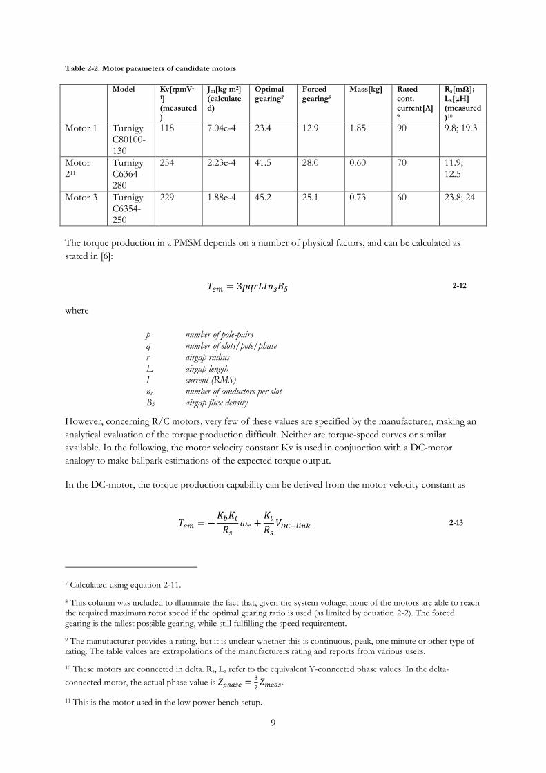
Table 2-2. Motor parameters of candidate motors
Model Kv[rpmV-
1] (measured)
Jm[kg m2] (calculated)
Optimal gearing7
Forced gearing8
Mass[kg] Rated cont. current[A]9
Rs[mΩ]; Ls[μH] (measured)10
Motor 1 Turnigy C80100-130
118 7.04e-4 23.4 12.9 1.85 90 9.8; 19.3
Motor 211
Turnigy C6364-280
254 2.23e-4 41.5 28.0 0.60 70 11.9; 12.5
Motor 3 Turnigy C6354-250
229 1.88e-4 45.2 25.1 0.73 60 23.8; 24
The torque production in a PMSM depends on a number of physical factors, and can be calculated as
stated in [6]:
2-12
where
p number of pole-pairs q number of slots/pole/phase r airgap radius L airgap length I current (RMS) ns number of conductors per slot Bδ airgap flux density
However, concerning R/C motors, very few of these values are specified by the manufacturer, making an
analytical evaluation of the torque production difficult. Neither are torque-speed curves or similar
available. In the following, the motor velocity constant Kv is used in conjunction with a DC-motor
analogy to make ballpark estimations of the expected torque output.
In the DC-motor, the torque production capability can be derived from the motor velocity constant as
2-13
7 Calculated using equation 2-11.
8 This column was included to illuminate the fact that, given the system voltage, none of the motors are able to reach the required maximum rotor speed if the optimal gearing ratio is used (as limited by equation 2-2). The forced gearing is the tallest possible gearing, while still fulfilling the speed requirement.
9 The manufacturer provides a rating, but it is unclear whether this is continuous, peak, one minute or other type of rating. The table values are extrapolations of the manufacturers rating and reports from various users.
10 These motors are connected in delta. Rs, Ls refer to the equivalent Y-connected phase values. In the delta-
connected motor, the actual phase value is
.
11 This is the motor used in the low power bench setup.
10
where
2-14
are the back emf constant and the torque constant, respectively. It shall be noted that equation 2-13
assumes limitless current capabilities, which is the case only at high speeds. The torque production in
relation to current is described by equation 2-15. [7]
2-15
Torque-speed curves were drawn for the candidate motors, along with the torque requirement. Since each
motor is previewed with an individual gearing, the same torque requirement at the wheel translates into
three different values, when evaluated at the motor shaft.
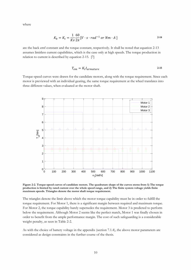
Figure 2-2. Torque-speed curves of candidate motors. The quadrature shape of the curves stems from 1) The torque production is limited by rated current over the whole speed range, and 2) The finite system voltage yields finite maximum speeds. Triangles denote the motor shaft torque requirement.
The triangles denote the limit above which the motor torque capability must be in order to fulfill the
torque requirement. For Motor 1, there is a significant margin between required and maximum torque.
For Motor 2, the torque capability barely supersedes the requirement. Motor 3 is predicted to perform
below the requirement. Although Motor 2 seems like the perfect match, Motor 1 was finally chosen in
order to benefit from the ample performance margin. The cost of such safeguarding is a considerable
weight penalty, as seen in Table 2-2.
As with the choice of battery voltage in the appendix (section 7.1.4), the above motor parameters are
considered as design constraints in the further course of the thesis.
0 100 200 300 400 500 600 700 800 900 1000 11000
1
2
3
4
5
6
7
8
9
r[rad/s]
Tm
[Nm
]
Motor 1
Motor 2
Motor 3
11
2.3 Thermal considerations in selecting the motor
The foreseen load cycle of this motor drive is simply: Full load for the time period required to ride up the
hill. Not only will the motor run at close to full load in a summer resort surrounding, it will at the same
time be running in its upper rpm range, i.e. the worst possible scenario from a heating perspective.
Power loss in an electrical motor can be stated as
2-16
where
PR resistive power loss PFW friction and windage loss PEH lamination eddy currents and hysteresis loss Ps switching frequency ripple loss Pstray losses not included above
and where PR=RsIRMS2 is dominant.
The resulting motor temperature rise depends on the thermal resistance of the motor to the surroundings
as
2-17
The thermal resistance can be influenced, and it seems likely that some kind of forced cooling system will
be necessary, which is beyond the scope of this thesis. As a temporary mitigation strategy, a temperature
sensor was fitted to the stator winding, and connected to the controller trip circuits.
2.4 Match between the motor and the power electronic converter
2.4.1 Current rating
The torque produced by the motor is proportional to the current supplied by the inverter to the motor.
The inverter must therefore be rated accordingly. In this case, looking at Motor 1 in Figure 2-2, the rating
of the inverter components should be equal to or above the current rating for this motor. The rating
finally chosen has a 50% safety margin, with reference to a general community of electronics and power
electronics designers and their experiences shared on various forums.
2.4.2 Voltage rating
The voltage rating must be chosen so that the voltage applied is equal to the highest expected back emf
from the motor, in addition to some margin for torque control. Torque is proportional to current, and the
significance of a voltage margin is illustrated by the following relation between the rate of change of
current (and hence torque), back emf and the applied voltage. (For reasons of clarity, the stator resistive
voltage drop has been neglected.)
2-18
If the applied voltage is too close to the back emf, controllability is lost.
12
The voltage rating finally chosen has a strong practical consideration component. The main issues are the
fact that the battery pack must be able to withstand very harsh treatment, without falling apart or falling
off the bike; and the voltage limitations of commonly available, reasonable priced and reasonably sized
electronics components. Voltage rating is strongly coupled to component size. Ideally, the battery pack
should also be water-resistant. The dimensioning system voltage is quantified in the appendix (section
7.1.4).
2.4.3 Switching frequency and motor inductance
The design trade-off when choosing switching frequency is switching losses versus steady-state motor
current ripple. Switching losses are easily quantified, and increase linearly with frequency. Motor current
ripple losses require a more complex analysis to quantify.
Commercially available R/C-controllers normally operate at <10 kHz switching frequency (100 μs period),
and are tightly rated for 50 VDC. On the contrary, a general rule of thumb in motor control is to keep the
switching frequency above the audible range, i.e. >20 kHz (50 μs period). Using the intended parameters
of this drive; vapplied=60.8 V, Lmotor=38.5 μH, (back emf)=vapplied/2 (i.e. half of maximum speed), fswitch=20
kHz and duty cycle=50%, equation 2-18 can be used to estimate the steady-state current ripple.
2-19
Resistive voltage drops in bulk filter capacitors, transistor switches and the motor itself will dampen this
ripple some. But the value remains at some 20-25% of rated motor current, which may be the source of
ripple torque. Without further consideration of the switching losses, a switching frequency of 25 kHz was
chosen. Again, the final decision is heavily influenced by practical considerations. From a software
perspective, it is convenient to couple the switching frequency with the frequency of execution of the
FOC algorithm. As will be discussed later, a FOC algorithm execution frequency of 20 kHz or above is
necessary.
2.5 Current limiting
Current control is inherent to the FOC algorithm. Details on the current controller, including parameter
tuning, is given in chapters below.
In addition to the software current control, comparators were installed to act instantly on overcurrent.
Whereas the software measures the current once each time the FOC algorithm is run – which is at some
20-30 kHz – the external comparator, being a slow model, has a response time of 1.3 μs. The external
overcurrent protection was set to trigger at considerably higher values than the software protection, so as
to provide a safety net when the software has failed to bound the current by control means.
13
3 Control of the PMSM
This chapter starts with an introduction to vector control of sensorless PMSMs. A practical case is then
considered, where the control algorithm is implemented and tested with a motor and a load. The case is
first simulated in software, and the simulation results are then verified in the actual test bench setup.
3.1 FOC – mimicking the DC-motor
The PMSM belongs to the general family of AC-motors. The sinusoidal voltages interact with the stator
windings to produce a rotating magnetic field in the air gap. Because of the non-linearity of a sinusoidal,
the control of such signals is inherently complicated. As a consequence, before the advent of FOC, any
AC-motor inverter was “a short-circuit waiting to happen” [3]. The general concept of FOC is to avoid
the ever-changing sinusoidal stator environment when making decisions about the control of the motor.
Instead, the stator signals are transformed through a number of operations, to finally appear as DC
quantities. A short and informative definition of FOC from [2] is cited here:
Vector control implies that an AC motor is forced to behave dynamically as a DC motor by the use of feedback control.
A popular description is to imagine one-self standing on the rotor, looking out over the air-gap towards
the stator. The three-phase sinusoidal stator currents produce a rotating magnetic field in the air-gap. But
from the position of the rotor, which is rotating at synchronous speed, this magnetic field is a DC
quantity. From the rotor view, motor control is a matter of DC quantities, and commonplace linear
control strategies can be employed.
In short, the three-phase mmf is transformed to a two-phase quantity. This quantity is then rotated using
the angle of the rotor vis-à-vis the stator, to align it with the rotor. The stator quantities are now evaluated
with the rotor as reference. They are said to be synchronous with the rotor, and being stated in the rotor
reference frame. A more in-depth treatment is given in later sections.
A conceptual level block diagram of the FOC control algorithm was adapted from [2], and is shown in
Figure 3-1. It can be read starting from the throttle input, which is a DC current reference (n.b. not a
speed reference). The input is compared to the actual DC current is (which is a transformation of the
actual three-phase AC currents going to the motor, as will be discussed in detail in later sections). The
difference between the two is fed to the PI-controller, and an output DC-voltage vs is decided. This
voltage is then fed to the motor by the inverter, again, after being transformed to a corresponding AC-
value. The angle estimation is necessary to keep track of the peak of the rotating magnetic field produced
by the rotor. Using this angle, the vs DC voltage vector can be applied wherever the AC-field phasor
happens to be at.
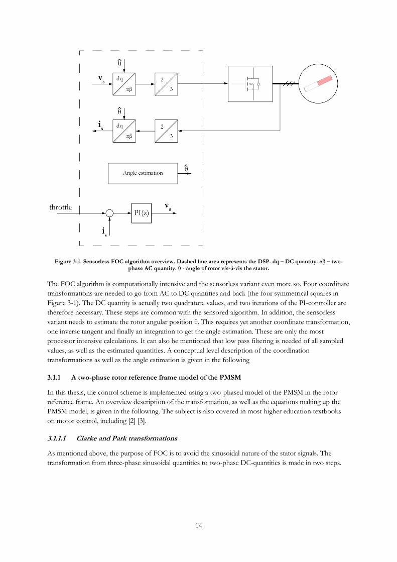
14
Figure 3-1. Sensorless FOC algorithm overview. Dashed line area represents the DSP. dq – DC quantity. αβ – two-phase AC quantity. θ - angle of rotor vis-á-vis the stator.
The FOC algorithm is computationally intensive and the sensorless variant even more so. Four coordinate
transformations are needed to go from AC to DC quantities and back (the four symmetrical squares in
Figure 3-1). The DC quantity is actually two quadrature values, and two iterations of the PI-controller are
therefore necessary. These steps are common with the sensored algorithm. In addition, the sensorless
variant needs to estimate the rotor angular position θ. This requires yet another coordinate transformation,
one inverse tangent and finally an integration to get the angle estimation. These are only the most
processor intensive calculations. It can also be mentioned that low pass filtering is needed of all sampled
values, as well as the estimated quantities. A conceptual level description of the coordination
transformations as well as the angle estimation is given in the following
3.1.1 A two-phase rotor reference frame model of the PMSM
In this thesis, the control scheme is implemented using a two-phased model of the PMSM in the rotor
reference frame. An overview description of the transformation, as well as the equations making up the
PMSM model, is given in the following. The subject is also covered in most higher education textbooks
on motor control, including [2] [3].
3.1.1.1 Clarke and Park transformations
As mentioned above, the purpose of FOC is to avoid the sinusoidal nature of the stator signals. The
transformation from three-phase sinusoidal quantities to two-phase DC-quantities is made in two steps.
15
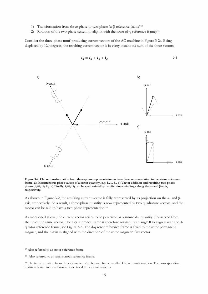
1) Transformation from three-phase to two-phase (α-β reference frame)12
2) Rotation of the two-phase system to align it with the rotor (d-q reference frame) 13
Consider the three-phase mmf-producing current vectors of the AC-machine in Figure 3-2a. Being
displaced by 120 degrees, the resulting current vector is in every instant the sum of the three vectors.
3-1
Figure 3-2. Clarke transformation from three-phase representation to two-phase representation in the stator reference frame. a) Instantaneous phase values of a stator quantity, e.g. ia, ib, ic. b) Vector addition and resulting two-phase phasor, is=ia+ib+ic. c) Finally, is=iα+iβ can be synthesized by two fictitious windings along the α- and β-axis, respectively.
As shown in Figure 3-2, the resulting current vector is fully represented by its projection on the α- and β-
axis, respectively. As a result, a three-phase quantity is now represented by two quadrature vectors, and the
motor can be said to have a two-phase representation.14
As mentioned above, the current vector seizes to be perceived as a sinusoidal quantity if observed from
the tip of the same vector. The α-β reference frame is therefore rotated by an angle θ to align it with the d-
q rotor reference frame, see Figure 3-3. The d-q rotor reference frame is fixed to the rotor permanent
magnet, and the d-axis is aligned with the direction of the rotor magnetic flux vector.
12 Also referred to as stator reference frame.
13 Also referred to as synchronous reference frame.
14 The transformation from three-phase to α-β reference frame is called Clarke transformation. The corresponding matrix is found in most books on electrical three-phase systems.

16
Figure 3-3. Park transformation from α-β to d-q reference frame by a transformation angle θ.
The Park transformation matrix is used to rotate the stationary α-β reference frame. This change of base is
here exemplified by the current vector transformation.
[
] [ ( ) ( )
( ) ( )] [
] 3-2
The three-phase motor is now represented with a two-phase equivalent, which rotates synchronously with
the rotor. The position of the rotor, θ, determines what voltages will eventually be applied to the three-
phased motor. The sensorless motor has no means of measuring and feeding the value of θ back to the
controller, and the estimation of this value is treated in the following.
3.1.1.2 Equations of the two-phase PMSM model
The magnets in R/C motors are of the surface mounted type. Since the reluctance of magnets is roughly
the same as in air, this implies that the inductance is the same in along both d- and q-axis.
The voltage equations of the PMSM in rotor reference frame are then obtained as
[
] [
] [
] [
] 3-3
Further, the electromagnetic torque developed by the motor is expressed as
3-4
3.1.2 The PLL-type estimator
There are two main strategies for estimating the position of the PMSM rotor. The first one uses injection
of high frequency voltages to detect the saliency variation of a salient PMSM. In the second strategy, valid
17
for medium and high speeds only15, the induced back emf is used to estimate the position [8]. A surface
mounted PMSM is characterized by its non-saliency, and only the second strategy can be considered for
the motor at hand.
The PLL16-type back emf estimator is well established as a promising method for position estimation of
the AC-motor [8]. A method of this type is presented in [9]. This method is analyzed and further
developed in [8], and a variant of the introductory presentation provided there is reproduced in the
following.
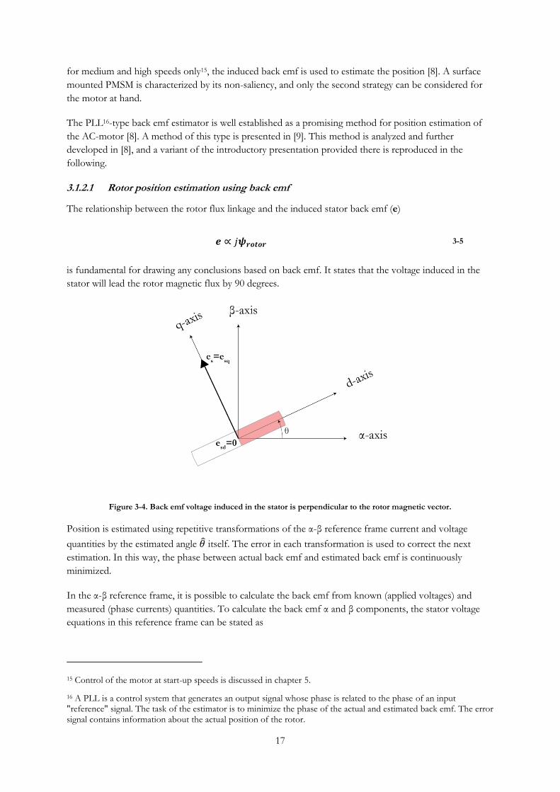
3.1.2.1 Rotor position estimation using back emf
The relationship between the rotor flux linkage and the induced stator back emf (e)
3-5
is fundamental for drawing any conclusions based on back emf. It states that the voltage induced in the
stator will lead the rotor magnetic flux by 90 degrees.
Figure 3-4. Back emf voltage induced in the stator is perpendicular to the rotor magnetic vector.
Position is estimated using repetitive transformations of the α-β reference frame current and voltage
quantities by the estimated angle itself. The error in each transformation is used to correct the next
estimation. In this way, the phase between actual back emf and estimated back emf is continuously
minimized.
In the α-β reference frame, it is possible to calculate the back emf from known (applied voltages) and
measured (phase currents) quantities. To calculate the back emf α and β components, the stator voltage
equations in this reference frame can be stated as
15 Control of the motor at start-up speeds is discussed in chapter 5.
16 A PLL is a control system that generates an output signal whose phase is related to the phase of an input "reference" signal. The task of the estimator is to minimize the phase of the actual and estimated back emf. The error signal contains information about the actual position of the rotor.
18
3-6
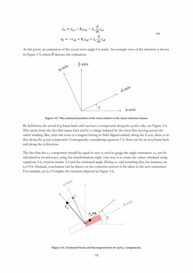
At this point, an estimation of the actual rotor angle θ is made. An example view of the situation is shown
in Figure 3-5, where denotes the estimation.
Figure 3-5. The estimated position of the rotor relative to the stator reference frame.
By definition, the actual d-q frame back emf can have a component along the q-axis only, see Figure 3-4.
This stems from the fact that stator back emf is a voltage induced by the rotor flux moving across the
stator winding. But, since the rotor is a magnet having its field aligned entirely along the d-axis, there is no
flux along the q-axis component. Consequently, considering equation 3-5, there can be no d-q frame back
emf along the d-direction.
The fact that the esd component should be equal to zero is used to gauge the angle estimation. esd can be
calculated in several ways, using the transformation angle. One way is to rotate the values obtained using
equations 3-6, rotation matrix 3-2 and the estimated angle. Doing so, and assuming that, for instance, an
êsd>0 is obtained, conclusions can be drawn on the corrective actions to be taken in the next estimation.
For example, an êsd>0 implies the situation depicted in Figure 3-6.
Figure 3-6. Estimated back emf decomposed into d- and q- components.
19
Clearly, in order to compensate for the non-zero êsd component, should be decreased, thus aligning the
estimated d-q frame with the actual rotor position θ. This information is used in the next estimation
cycle. In this way, the phase between estimated and actual back emf is locked, or minimized, in a
reiterative loop.
Template software for a PLL-based PMSM back emf and angle estimator was found in [10], which was
adapted for the present application.
3.1.3 Field-weakening
Field-weakening17 is used to suppress the permanent magnet flux, with the purpose of decreasing the
induced back emf, as described by equation 3-5. In this way, it is possible to run the motor at speeds
above base speed, i.e. where the back emf would normally equal the q-axis stator voltage. The method
consists in injecting a current in the negative d-axis direction, and thereby creating a stator magnetic flux
counteracting the flux of the permanent magnet.
Field-weakening will not be used in this application, for two reasons. First of all, SMPMs have an
inherently large air gap, due to the fact that the magnets have approximately the same permeance as air.
This gives the magnetic circuit highly non-linear properties, which are difficult to control. Interior
permanent magnet machines are generally considered superior to the SMPM for field-weakening
operation. [3]
Secondly, field-weakening can only be performed at the cost of torque. Looking at the stator current
vector in Figure 3-2, it is realized that an increasing d-axis component leads to a corresponding decrease in
q-axis direction, given that inverter is running at full voltage output. In this application, the nature of the
predominant load – uphill propulsion – implies full torque at full speed. In this case, it makes little sense
to trade torque for speed.
When field-weakening is not available, the system voltage and the motor drive gearing must be chosen to
allow for target speed to be less than the rotor base speed.
3.2 Design of the current controller
Having established a two-phase, synchronous equivalent of the PMSM, there is now enough input to
derive a suitable current controller. The circuits to be controlled were reproduced from [3].
17 Also referred to as flux weakening.
20
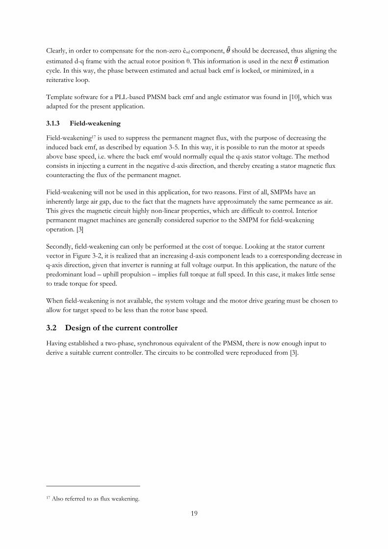
Figure 3-7. Dynamic equivalent circuits of the PMSM, neglecting core losses. a) q-axis equivalent circuit. b) d-axis equivalent circuit.
In this view, the so called cross-coupling between the d- and q-axis is clear. In the q-axis circuit, there is a
component that depends on the d-axis current magnitude, and vice versa. According to most authors, this
should be compensated for in the current controller (see e.g. [2] [3] [8]). However, in this application,
given the moderate power requirements, and the fact that the motor is non-salient, no such compensation
is necessary. [11]
In the following, a model of the experimental setup motor and controller circuits is derived and simulated
in simulation software. Then the same tests are conducted on the actual experimental setup, and the two
sets of results are checked for discrepancies. The purpose is to establish a method for tuning of the PI-
controllers, which can then be more or less seamlessly ported to the larger drive which will actually be
used on the test bike.
3.2.1 PI-tuning by simulation
By inspection of the circuits in Figure 3-7 (or the d-q voltage equations 3-3), the resulting transfer
function is of first order, and PI control is sufficient. For such a system, there is an analytical relation
between the control system bandwidth, b, and the current rise time18, tr. [2]
( ) 3-7
In the following tests, the PWM-frequency was chosen to be 20 kHz. The resulting expected rise time is
( )
3-8
18 Rise time is in this expression defined as the time it takes for the value to rise from 20% to 80% of its settling value.
21
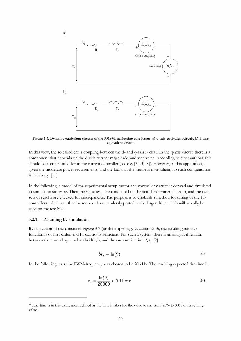
A model of the control system for one phase was implemented in Simulink, see Figure 3-8. In the
following, the various gains and transfer functions will be derived, and the circuit will be simulated for a
torque demand step to verify assumptions made.
Figure 3-8. Simplified per-phase control system, neglecting the influences of back emf, cross-coupling and inherent motor, controller and sensor response time delays.
3.2.1.1 Reference block
This is the throttle. In motor control, there is often an inner control loop for currents, and an outer,
slower control loop, for speed control. In this application, however, the rider is responsible for speed
control, and the throttle will immediately control the torque reference fed to the system. In equation 3-4,
it is seen that torque is directly proportional to the q-axis current. Hence, torque demand is proportional
to a current demand.
In the simulation, an 8A current demand step is given. To include the actual DSP implementation, the
physical current sensors and the controller-inverter gain in the simulation; the reference is scaled to its
internal representation in the DSP. In the low-power experimental setup, the full throttle has a 15 bits
resolution, corresponding to a 62.5A current demand. Hence, the reference step is set to
3.2.1.2 PI controller block
The PI-controller transfer function in the frequency domain is given as
( )
3-9
The gains were chosen in accordance with the internal model control design approach, as discussed in [12].
Stator resistance and inductance values from the low power experimental setup were used, see section 7.2
for details.
3-10
3-11
In the Simulink PI-block, the time-domain was set to discrete-time, with a sample frequency equal to the
PWM-frequency. The output of the block was limited to √ , which is the maximum allowable
22
voltage output considering the limitation of the SVM scheme discussed above (215 being equal to the DC-
link voltage).
3.2.1.3 Controller-inverter block
The simulation was programed for a 36V DC-link voltage, which corresponds to a 215 integer output to
the inverter. The gain is hence
3.2.1.4 Motor block
Taking the Laplace transform of any of the circuits in Figure 3-7, assuming zero initial conditions and
disregarding back emf and cross-coupling, the following voltage equation results:
( ) ( ) ( ) 3-12
Rs and Ls are taken from the low power experimental setup motor. The corresponding transfer function is
( )
( )
⁄
⁄
3.2.1.5 Current sensor block
The gain is
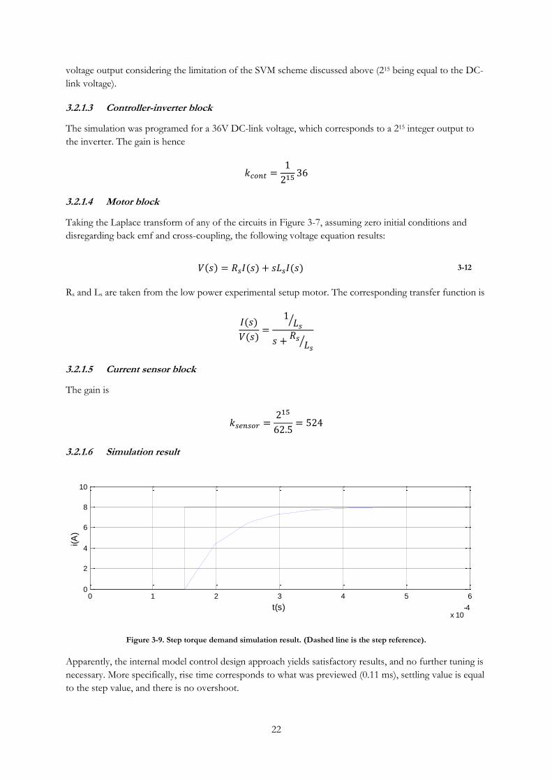
3.2.1.6 Simulation result
Figure 3-9. Step torque demand simulation result. (Dashed line is the step reference).
Apparently, the internal model control design approach yields satisfactory results, and no further tuning is
necessary. More specifically, rise time corresponds to what was previewed (0.11 ms), settling value is equal
to the step value, and there is no overshoot.
0 1 2 3 4 5 6
x 10-4
0
2
4
6
8
10
t(s)
i(A
)
23
3.2.2 The control strategy
Using FOC, it is possible to decouple the torque and flux production in the AC-motor, which can be used
to derive different control strategies. In [3], seven common strategies for d-q control are analyzed in-
depth, namely
1. Constant torque angle control (zero d-axis current control)
2. Unity power factor control
3. Constant mutual air gap flux-linkages control
4. Angle control of air gap flux and current phasors
5. Optimum torque per ampere control
6. Constant loss based maximum torque speed boundary control
7. Minimum loss (maximum efficiency) control
For this particular application, it is important to notice the non-saliency of the rotor magnet configuration,
which limits many of the possibilities. The reason for this is the fact that the object of control in the above
strategies is often the torque equation. For a non-salient rotor, equation 3-4 holds. The same equation for
a salient rotor is more complicated,
[ ( ) ] 3-13
and lends itself to a broader palette of manipulation. The saliency of such motors manifests itself in the
difference in magnitude of the d- and q-axis inductances. (2), (3), (4) and (5) are valid for salient motors
only, and are therefore discarded.
Control strategy (6) has the objective of limiting the loss to a thermally acceptable value, hence
safeguarding the thermal robustness of the motor. As further described in paragraph 2.3, such
considerations are considered beyond the scope of this thesis. (7) has its greatest benefits in efficiency
sensitive applications such as ventilation, air conditioning and home appliances (washers, freezers, vacuum
cleaners, etc.) [3]. Control strategy (1) Constant torque angle control was chosen for this application.
3.2.2.1 Limitations of the constant torque angle control strategy
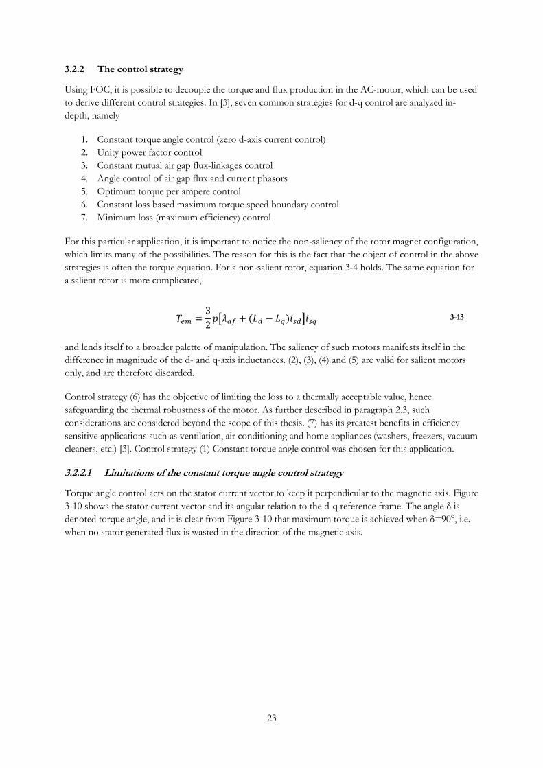
Torque angle control acts on the stator current vector to keep it perpendicular to the magnetic axis. Figure
3-10 shows the stator current vector and its angular relation to the d-q reference frame. The angle δ is
denoted torque angle, and it is clear from Figure 3-10 that maximum torque is achieved when δ=90°, i.e.
when no stator generated flux is wasted in the direction of the magnetic axis.
24
Figure 3-10. Constant torque angle control and the resulting stator current phasor is orientation in the rotor reference frame.
The torque equation for non-salient motors, equation 3-4 (repeated here for clarity), supports this
observation. Only the q-axis current contributes to the torque production.
In the following, the analysis presented in [3] of the constant torque angle control strategy is used for the
motor drive at hand. The fact that d-axis current is regulated to zero renders this strategy unusable for
drives requiring flux weakening operation. But for the application at hand, this does not pose any
limitation, as discussed in section 3.1.3. A potentially more acute problem is the deteriorating power factor
and torque at high currents and speeds, respectively. This is discussed in the following.
It is informative to return to the d-q reference frame voltage equations. If equations 3-3 are adapted for
the constant torque angle control strategy (isd=0, isq=is), and simplified to reflect steady-state (
), they
can be re-stated as
3-14
A limitation arises in the second equation, where the d-axis voltage is affected by both rotor speed and
stator current. As seen in Figure 3-10, an increasing vsd comes at the cost of a decrease in vsq. The power
factor is affected, and so is the speed capability. The first of equations 3-14 shows that the q-axis voltage is
used both to overcome the back emf, as well as to produce torque. High speeds and high currents are
therefore possible impediments to attain target torque and speed.
The following analysis is conducted in a per unit system, which enables the comparison of several
variables simultaneously, as well as to exhibit the resulting magnitudes directly in relation to relevant
system magnitudes. The derivation of the base variables are presented in section 7.3. Some important base
values are Ib (set equal to motor rated continuous current), Tb (equal to Ib) and ωb (value derived from
base voltage and base magnetic flux, no evident system parameter relation).
25
The situation can be analyzed using the stator voltage component equation
√( ) ( ) 3-15
and re-writing it in the variables of interest. First, Vs is normalized, and expressed in terms of equations
3-14.
√( ) ( ) ( ) 3-16
The limiting condition (equation 3-15) is now expressed in terms of the relevant values of stator current
and rotor speed. By rearranging equation 3-16, and realizing from Figure 3-10 that the power factor can be
stated in terms of the steady-state stator voltage vector and its q-axis component, it can be expressed as
√
( )
(
)
3-17
Further, equation 3-16 can be solved for Isn. In this way, a relationship between (normalized) rotor speed
and torque capability (equal to the normalized current) is established, for a certain maximum stator
voltage.
√
(
)
3-18
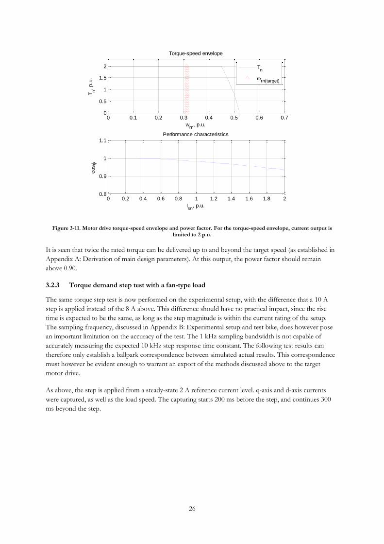
Equations 3-17 and 3-18 are now analyzed for
√ ⁄ .
26
Figure 3-11. Motor drive torque-speed envelope and power factor. For the torque-speed envelope, current output is limited to 2 p.u.
It is seen that twice the rated torque can be delivered up to and beyond the target speed (as established in
Appendix A: Derivation of main design parameters). At this output, the power factor should remain
above 0.90.
3.2.3 Torque demand step test with a fan-type load
The same torque step test is now performed on the experimental setup, with the difference that a 10 A
step is applied instead of the 8 A above. This difference should have no practical impact, since the rise
time is expected to be the same, as long as the step magnitude is within the current rating of the setup.
The sampling frequency, discussed in Appendix B: Experimental setup and test bike, does however pose
an important limitation on the accuracy of the test. The 1 kHz sampling bandwidth is not capable of
accurately measuring the expected 10 kHz step response time constant. The following test results can
therefore only establish a ballpark correspondence between simulated actual results. This correspondence
must however be evident enough to warrant an export of the methods discussed above to the target
motor drive.
As above, the step is applied from a steady-state 2 A reference current level. q-axis and d-axis currents
were captured, as well as the load speed. The capturing starts 200 ms before the step, and continues 300
ms beyond the step.
0 0.1 0.2 0.3 0.4 0.5 0.6 0.70
0.5
1
1.5
2
wrn
, p.u.
Tn,
p.u
.
Torque-speed envelope
Tn
rn(target)
0 0.2 0.4 0.6 0.8 1 1.2 1.4 1.6 1.8 20.8
0.9
1
1.1
Isn
, p.u.
cos
Performance characteristics
27
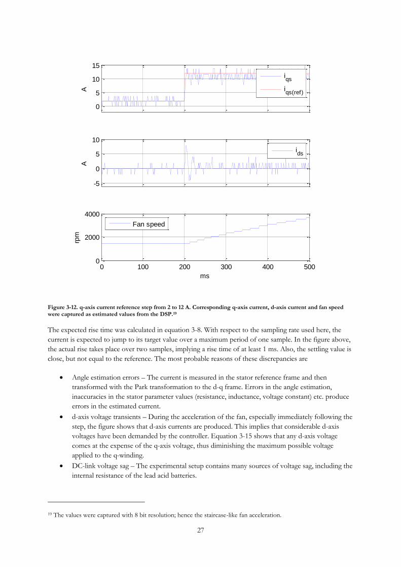
Figure 3-12. q-axis current reference step from 2 to 12 A. Corresponding q-axis current, d-axis current and fan speed were captured as estimated values from the DSP.19
The expected rise time was calculated in equation 3-8. With respect to the sampling rate used here, the
current is expected to jump to its target value over a maximum period of one sample. In the figure above,
the actual rise takes place over two samples, implying a rise time of at least 1 ms. Also, the settling value is
close, but not equal to the reference. The most probable reasons of these discrepancies are
Angle estimation errors – The current is measured in the stator reference frame and then
transformed with the Park transformation to the d-q frame. Errors in the angle estimation,
inaccuracies in the stator parameter values (resistance, inductance, voltage constant) etc. produce
errors in the estimated current.
d-axis voltage transients – During the acceleration of the fan, especially immediately following the
step, the figure shows that d-axis currents are produced. This implies that considerable d-axis
voltages have been demanded by the controller. Equation 3-15 shows that any d-axis voltage
comes at the expense of the q-axis voltage, thus diminishing the maximum possible voltage
applied to the q-winding.
DC-link voltage sag – The experimental setup contains many sources of voltage sag, including the
internal resistance of the lead acid batteries.
19 The values were captured with 8 bit resolution; hence the staircase-like fan acceleration.
0
5
10
15
A
iqs
iqs(ref)
-5
0
5
10
A
ids
0 100 200 300 400 5000
2000
4000
ms
rpm
Fan speed
28
Ground bounce – The experimental setup breadboard, and the long cables interconnecting
current sensors, gate drive signals etc. produce a considerable ground bounce, sometimes above 1
V. This is likely to negatively influence the phase current measurements, amongst others, and will
deteriorate the performance of the setup.
Software filter cut-off frequency set too low. It was only later realized that the cut-off frequency
was adjusted too tightly, and the rapid acceleration of the fan was not accurately followed by the
algorithm. The consequence is that the rotor angle estimation deteriorates during the speed
transient.
In view of this, grosso modo, the above step results are considered satisfactory and in line with the expected
outcome. The PI-tuning strategy presented in earlier paragraphs is therefore likely to produce satisfactory
result also on the target application.
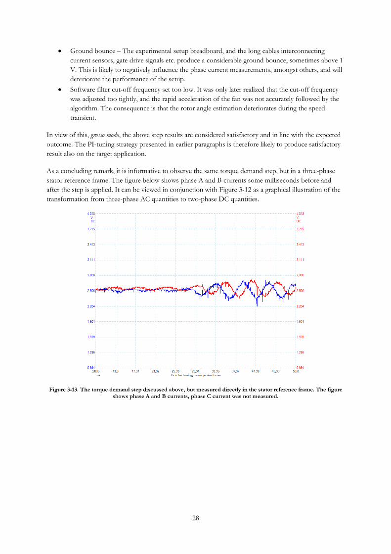
As a concluding remark, it is informative to observe the same torque demand step, but in a three-phase
stator reference frame. The figure below shows phase A and B currents some milliseconds before and
after the step is applied. It can be viewed in conjunction with Figure 3-12 as a graphical illustration of the
transformation from three-phase AC quantities to two-phase DC quantities.
Figure 3-13. The torque demand step discussed above, but measured directly in the stator reference frame. The figure shows phase A and B currents, phase C current was not measured.
29
4 Prototyping
This chapter is concerned with the steps that were taken to prototype the actual controller-inverter to be
used on the bike. It is included to bridge the gap between the hypotheses made about control algorithms,
power requirements, etc. and the practical results that will be produced and analyzed in later chapters. The
presentation is made in a qualitative fashion, with focus on the process and some of the major
electrotechnical and electromagnetical design aspects that were encountered along the way, rather than on
components, data sheets and manufacturer application notes.
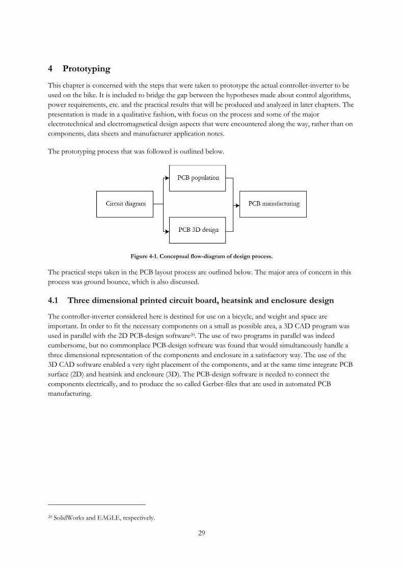
The prototyping process that was followed is outlined below.
Figure 4-1. Conceptual flow-diagram of design process.
The practical steps taken in the PCB layout process are outlined below. The major area of concern in this
process was ground bounce, which is also discussed.
4.1 Three dimensional printed circuit board, heatsink and enclosure design
The controller-inverter considered here is destined for use on a bicycle, and weight and space are
important. In order to fit the necessary components on a small as possible area, a 3D CAD program was
used in parallel with the 2D PCB-design software20. The use of two programs in parallel was indeed
cumbersome, but no commonplace PCB-design software was found that would simultaneously handle a
three dimensional representation of the components and enclosure in a satisfactory way. The use of the
3D CAD software enabled a very tight placement of the components, and at the same time integrate PCB
surface (2D) and heatsink and enclosure (3D). The PCB-design software is needed to connect the
components electrically, and to produce the so called Gerber-files that are used in automated PCB
manufacturing.
20 SolidWorks and EAGLE, respectively.

30
Figure 4-2. 3D model of the PCB.
Figure 4-3. Integration of an aluminum L-bar heatsink to thermally couple the transistors and the metallic enclosure.
4.2 Ground bounce
Ground bounce is when a voltage potential arises between two points on the same ground plane. The
reason for this is inductance, which is why ground bounce can reach unexpectedly high values even in low
power, low voltage applications, from mV to tens of volts. The governing equation is
4-1
and it is hence the rate of change in the current rather than the actual current magnitude that gives rise to
the voltage spikes. Serious ground bounce can therefore be caused by both power magnitude currents and
signal path currents21. In any inverter, the current is switched on and off several thousand times per
second, and the di/dt induced ground bounce, if left unchecked, is likely to be high. The situation for the
inverter in this application was analyzed through modeling, and a tentative mitigation strategy was
formulated.
21 [24] contains a graphical and excellent review of this phenomena, as well as outline mitigation strategies.
Power transistors
Bulk filter capacitors
DSP Current sensors
31
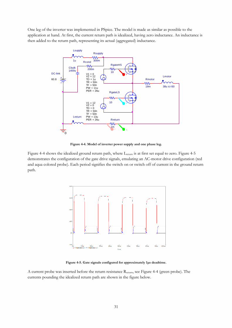
One leg of the inverter was implemented in PSpice. The model is made as similar as possible to the
application at hand. At first, the current return path is idealized, having zero inductance. An inductance is
then added to the return path, representing its actual (aggregated) inductance.
Figure 4-4. Model of inverter power supply and one phase leg.
Figure 4-4 shows the idealized ground return path, where Lreturn is at first set equal to zero. Figure 4-5
demonstrates the configuration of the gate drive signals, emulating an AC-motor drive configuration (red
and aqua colored probe). Each period signifies the switch on or switch off of current in the ground return
path.
Figure 4-5. Gate signals configured for approximately 1μs deadtime.
A current probe was inserted before the return resistance Rreturn, see Figure 4-4 (green probe). The
currents pounding the idealized return path are shown in the figure below.
TD = 0
TF = 50nPW = 13uPER = 26u
V1 = 12
TR = 50n
V2 = 0
RgateLS
10
Lsupply
1u
Cbulk1400u
Rsupply
300m
Rreturn
1m
Rcond
200m
Lreturn
V
V I
V
RgateHS
10DC-link
60.8
0
TD = 1u
TF = 50nPW = 11uPER = 26u
V1 = 0
TR = 50n
V2 = 12Rmotor
19m
Lmotor
38u ic=50
32
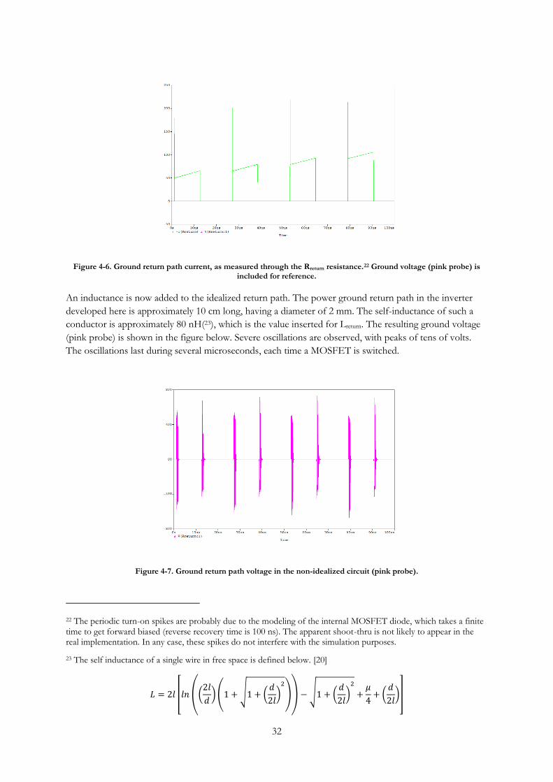
Figure 4-6. Ground return path current, as measured through the Rreturn resistance.22 Ground voltage (pink probe) is included for reference.
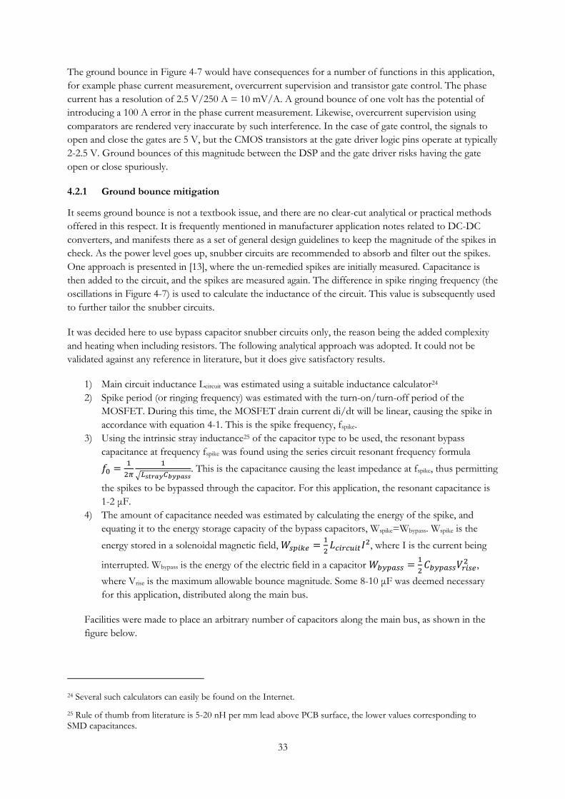
An inductance is now added to the idealized return path. The power ground return path in the inverter
developed here is approximately 10 cm long, having a diameter of 2 mm. The self-inductance of such a
conductor is approximately 80 nH(23), which is the value inserted for Lreturn. The resulting ground voltage
(pink probe) is shown in the figure below. Severe oscillations are observed, with peaks of tens of volts.
The oscillations last during several microseconds, each time a MOSFET is switched.
Figure 4-7. Ground return path voltage in the non-idealized circuit (pink probe).
22 The periodic turn-on spikes are probably due to the modeling of the internal MOSFET diode, which takes a finite time to get forward biased (reverse recovery time is 100 ns). The apparent shoot-thru is not likely to appear in the real implementation. In any case, these spikes do not interfere with the simulation purposes.
23 The self inductance of a single wire in free space is defined below. [20]
[
(
(
)( √ (
)
)
)
√ (
)
(
)]
33
The ground bounce in Figure 4-7 would have consequences for a number of functions in this application,
for example phase current measurement, overcurrent supervision and transistor gate control. The phase
current has a resolution of 2.5 V/250 A = 10 mV/A. A ground bounce of one volt has the potential of
introducing a 100 A error in the phase current measurement. Likewise, overcurrent supervision using
comparators are rendered very inaccurate by such interference. In the case of gate control, the signals to
open and close the gates are 5 V, but the CMOS transistors at the gate driver logic pins operate at typically
2-2.5 V. Ground bounces of this magnitude between the DSP and the gate driver risks having the gate
open or close spuriously.
4.2.1 Ground bounce mitigation
It seems ground bounce is not a textbook issue, and there are no clear-cut analytical or practical methods
offered in this respect. It is frequently mentioned in manufacturer application notes related to DC-DC
converters, and manifests there as a set of general design guidelines to keep the magnitude of the spikes in
check. As the power level goes up, snubber circuits are recommended to absorb and filter out the spikes.
One approach is presented in [13], where the un-remedied spikes are initially measured. Capacitance is
then added to the circuit, and the spikes are measured again. The difference in spike ringing frequency (the
oscillations in Figure 4-7) is used to calculate the inductance of the circuit. This value is subsequently used
to further tailor the snubber circuits.
It was decided here to use bypass capacitor snubber circuits only, the reason being the added complexity
and heating when including resistors. The following analytical approach was adopted. It could not be
validated against any reference in literature, but it does give satisfactory results.
1) Main circuit inductance Lcircuit was estimated using a suitable inductance calculator24
2) Spike period (or ringing frequency) was estimated with the turn-on/turn-off period of the
MOSFET. During this time, the MOSFET drain current di/dt will be linear, causing the spike in
accordance with equation 4-1. This is the spike frequency, fspike.
3) Using the intrinsic stray inductance25 of the capacitor type to be used, the resonant bypass
capacitance at frequency fspike was found using the series circuit resonant frequency formula
√ . This is the capacitance causing the least impedance at fspike, thus permitting
the spikes to be bypassed through the capacitor. For this application, the resonant capacitance is
1-2 μF.
4) The amount of capacitance needed was estimated by calculating the energy of the spike, and
equating it to the energy storage capacity of the bypass capacitors, Wspike=Wbypass. Wspike is the
energy stored in a solenoidal magnetic field,
, where I is the current being
interrupted. Wbypass is the energy of the electric field in a capacitor
,
where Vrise is the maximum allowable bounce magnitude. Some 8-10 μF was deemed necessary
for this application, distributed along the main bus.
Facilities were made to place an arbitrary number of capacitors along the main bus, as shown in the
figure below.
24 Several such calculators can easily be found on the Internet.
25 Rule of thumb from literature is 5-20 nH per mm lead above PCB surface, the lower values corresponding to SMD capacitances.

34
Figure 4-8. Snubber capacitor placement along main bus.
4.2.2 Bulk filter capacitance
Whereas the DC-link inductance in Figure 4-4 might be as high as 1-2 μH, the stray inductance of the
bulk capacitance Cbulk can be measured in tens of nanohenries. This implies that, during a switching event,
rapid changes of current will be supplied by the capacitors alone. The capacitance needed during one
switching cycle can be calculated using the definition of capacitance.
( )
where Iswitching=100 A, dtswitching=40 μs, duty cycle=50% and allowable main bus voltage drop ΔVbus=1 V.
In this application 6*220=1320 μF was finally used, due to space restrictions.
35
5 Results and conclusion
5.1 Results
5.1.1 Maximum no-load motor speed
The maximum electrical rotor speed at 30 kHz sampling frequency is 44 000 e-rpm (considering the seven
magnetic pole-pairs of the motor). The period at 30 kHz frequency is 33 μs, which is the highest possible
frequency, considering that the FOC algorithm takes approximately 28 μs to execute.
It seems that, beyond 44 000 e-rpm, the algorithm can no longer resolve the back emf into a position, and
the θ angle estimation fails. 44 000 e-rpm equals 733 e-rps, and the period for one electrical revolution
(corresponding to one period of the back emf-curve in Figure 2-1) is approximately 1.36 ms. Considering
the sampling period of 33 μs, this implies the algorithm needs approximately 41 samples per cycle to
accurately reconstruct the back emf. The maximum attainable speed is probably higher, should filter,
motor, PI-controller parameters, etc. be even more finely tuned.
Using the prescribed gearing ratio of 12.7, and a maximum rotor speed of 5000 rpm, a maximum road
speed of 13.6 ms-1 (48.9 kmh-1) is possible.
5.1.2 Power factor at nominal load
A full-throttle speed test was carried out on a flat, paved surface, with the purpose of verifying the vsd/vsq
relationship, i.e. the amount of the stator voltage vector that was used to counter the motor back emf at
maximum rotor speed, and how much was wasted in the cross-coupling described in section 3.2.2.1
Limitations of the constant torque angle control strategy. The expected mechanical rotor speed in the
idealized case where the entire stator voltage vector is applied along the q-axis (i.e. to counteract back emf)
is
√
⁄ √
⁄
A road speed of 31.5 kmh-1 was measured26 at full throttle. Translated to rotor mechanical speed, this
implies
As expected at this load, this indicates that the stator voltage vector is practically aligned with the stator
current vector, and the power factor is close to unity, as expected.
5.1.3 Hill climbing capability
This motor drive was designed to climb a graveled path of a certain incline at a certain speed
corresponding to the characteristics of a mountain resort lift shuttle service road, as specified in section
7.1. The best way to verify the adherence of the drive to these specifications is of course to make a test
run on the actual mountain side, or re-create these exact conditions. This was not possible, and a more
26 The overall gearing in this setup was 16.5, which is considerably higher than what was pre-viewed. At the time of the test, the needed mechanical parts for a correct gearing were not yet available.
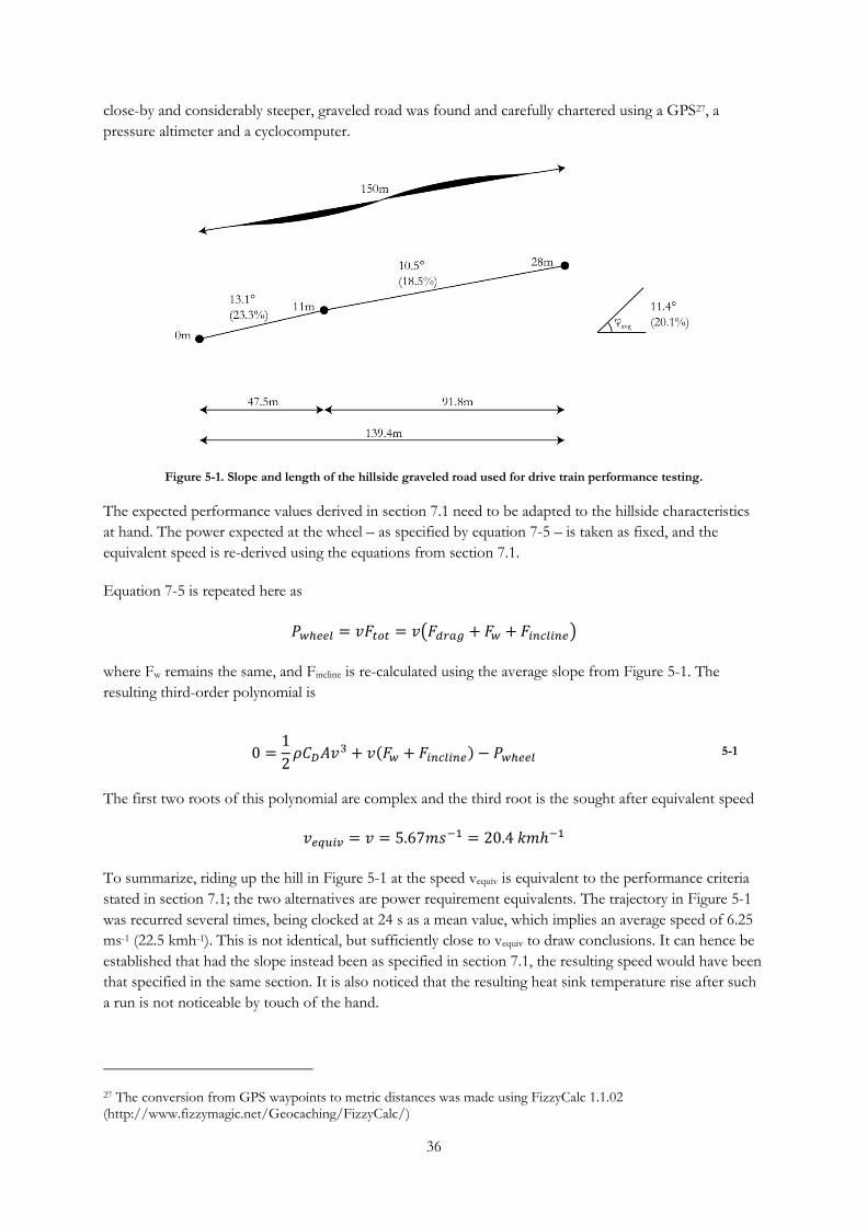
36
close-by and considerably steeper, graveled road was found and carefully chartered using a GPS27, a
pressure altimeter and a cyclocomputer.
Figure 5-1. Slope and length of the hillside graveled road used for drive train performance testing.
The expected performance values derived in section 7.1 need to be adapted to the hillside characteristics
at hand. The power expected at the wheel – as specified by equation 7-5 – is taken as fixed, and the
equivalent speed is re-derived using the equations from section 7.1.
Equation 7-5 is repeated here as
( )
where Fw remains the same, and Fincline is re-calculated using the average slope from Figure 5-1. The
resulting third-order polynomial is
( ) 5-1
The first two roots of this polynomial are complex and the third root is the sought after equivalent speed
To summarize, riding up the hill in Figure 5-1 at the speed vequiv is equivalent to the performance criteria
stated in section 7.1; the two alternatives are power requirement equivalents. The trajectory in Figure 5-1
was recurred several times, being clocked at 24 s as a mean value, which implies an average speed of 6.25
ms-1 (22.5 kmh-1). This is not identical, but sufficiently close to vequiv to draw conclusions. It can hence be
established that had the slope instead been as specified in section 7.1, the resulting speed would have been
that specified in the same section. It is also noticed that the resulting heat sink temperature rise after such
a run is not noticeable by touch of the hand.
27 The conversion from GPS waypoints to metric distances was made using FizzyCalc 1.1.02 (http://www.fizzymagic.net/Geocaching/FizzyCalc/)
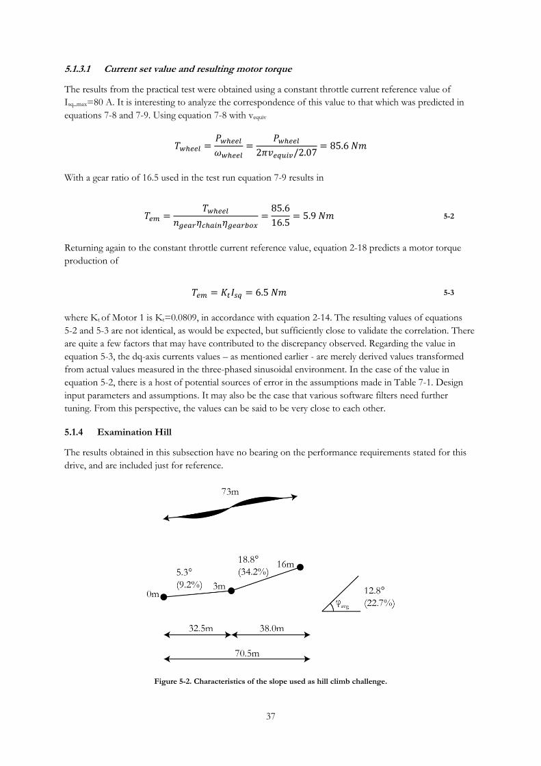
37
5.1.3.1 Current set value and resulting motor torque
The results from the practical test were obtained using a constant throttle current reference value of
Isq_max=80 A. It is interesting to analyze the correspondence of this value to that which was predicted in
equations 7-8 and 7-9. Using equation 7-8 with vequiv
With a gear ratio of 16.5 used in the test run equation 7-9 results in
5-2
Returning again to the constant throttle current reference value, equation 2-18 predicts a motor torque
production of
5-3
where Kt of Motor 1 is Kt=0.0809, in accordance with equation 2-14. The resulting values of equations
5-2 and 5-3 are not identical, as would be expected, but sufficiently close to validate the correlation. There
are quite a few factors that may have contributed to the discrepancy observed. Regarding the value in
equation 5-3, the dq-axis currents values – as mentioned earlier - are merely derived values transformed
from actual values measured in the three-phased sinusoidal environment. In the case of the value in
equation 5-2, there is a host of potential sources of error in the assumptions made in Table 7-1. Design
input parameters and assumptions. It may also be the case that various software filters need further
tuning. From this perspective, the values can be said to be very close to each other.
5.1.4 Examination Hill
The results obtained in this subsection have no bearing on the performance requirements stated for this
drive, and are included just for reference.
Figure 5-2. Characteristics of the slope used as hill climb challenge.
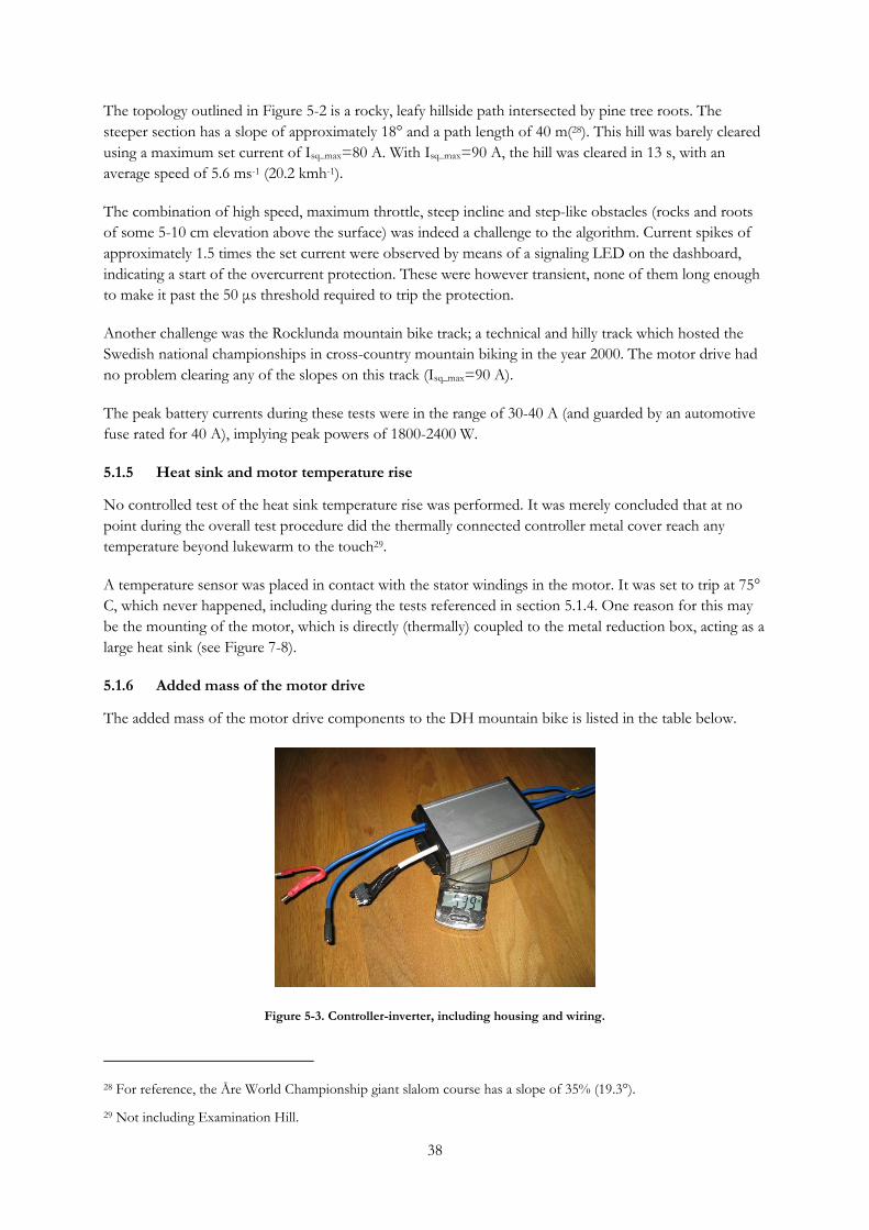
38
The topology outlined in Figure 5-2 is a rocky, leafy hillside path intersected by pine tree roots. The
steeper section has a slope of approximately 18° and a path length of 40 m(28). This hill was barely cleared
using a maximum set current of Isq_max=80 A. With Isq_max=90 A, the hill was cleared in 13 s, with an
average speed of 5.6 ms-1 (20.2 kmh-1).
The combination of high speed, maximum throttle, steep incline and step-like obstacles (rocks and roots
of some 5-10 cm elevation above the surface) was indeed a challenge to the algorithm. Current spikes of
approximately 1.5 times the set current were observed by means of a signaling LED on the dashboard,
indicating a start of the overcurrent protection. These were however transient, none of them long enough
to make it past the 50 μs threshold required to trip the protection.
Another challenge was the Rocklunda mountain bike track; a technical and hilly track which hosted the
Swedish national championships in cross-country mountain biking in the year 2000. The motor drive had
no problem clearing any of the slopes on this track (Isq_max=90 A).
The peak battery currents during these tests were in the range of 30-40 A (and guarded by an automotive
fuse rated for 40 A), implying peak powers of 1800-2400 W.
5.1.5 Heat sink and motor temperature rise
No controlled test of the heat sink temperature rise was performed. It was merely concluded that at no
point during the overall test procedure did the thermally connected controller metal cover reach any
temperature beyond lukewarm to the touch29.
A temperature sensor was placed in contact with the stator windings in the motor. It was set to trip at 75°
C, which never happened, including during the tests referenced in section 5.1.4. One reason for this may
be the mounting of the motor, which is directly (thermally) coupled to the metal reduction box, acting as a
large heat sink (see Figure 7-8).
5.1.6 Added mass of the motor drive
The added mass of the motor drive components to the DH mountain bike is listed in the table below.
Figure 5-3. Controller-inverter, including housing and wiring.
28 For reference, the Åre World Championship giant slalom course has a slope of 35% (19.3°).
29 Not including Examination Hill.
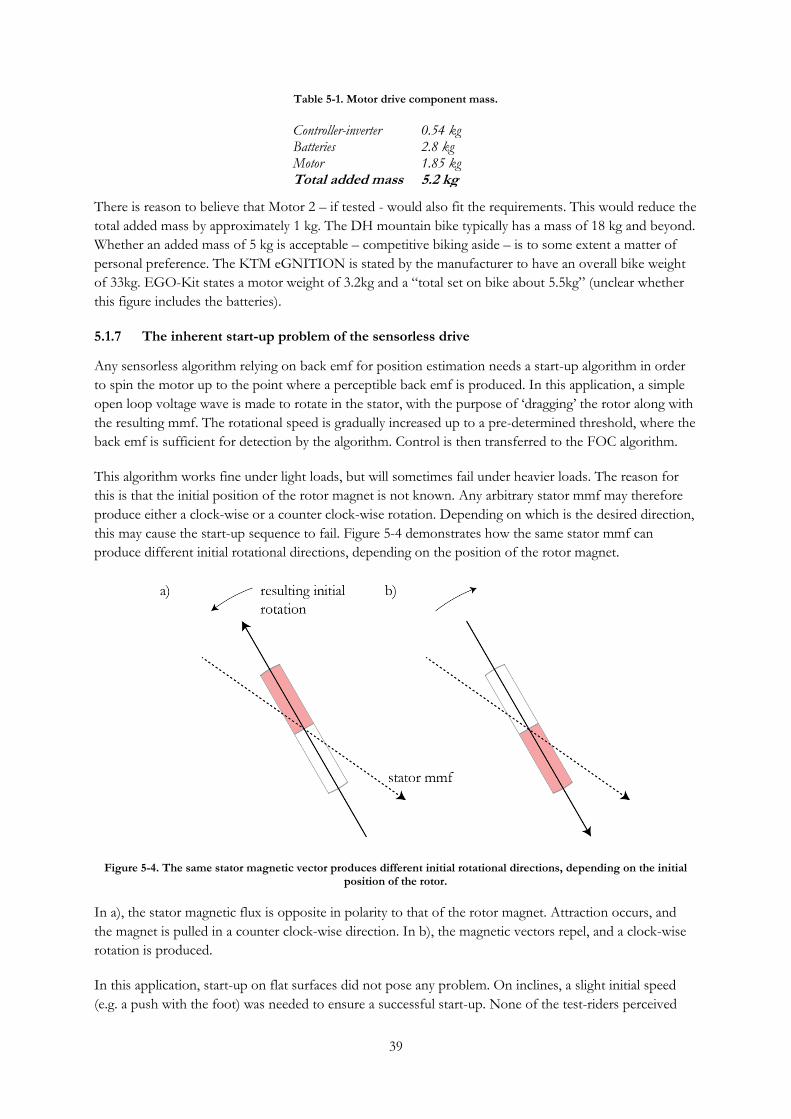
39
Table 5-1. Motor drive component mass.
Controller-inverter 0.54 kg Batteries 2.8 kg Motor 1.85 kg Total added mass 5.2 kg
There is reason to believe that Motor 2 – if tested - would also fit the requirements. This would reduce the
total added mass by approximately 1 kg. The DH mountain bike typically has a mass of 18 kg and beyond.
Whether an added mass of 5 kg is acceptable – competitive biking aside – is to some extent a matter of
personal preference. The KTM eGNITION is stated by the manufacturer to have an overall bike weight
of 33kg. EGO-Kit states a motor weight of 3.2kg and a “total set on bike about 5.5kg” (unclear whether
this figure includes the batteries).
5.1.7 The inherent start-up problem of the sensorless drive
Any sensorless algorithm relying on back emf for position estimation needs a start-up algorithm in order
to spin the motor up to the point where a perceptible back emf is produced. In this application, a simple
open loop voltage wave is made to rotate in the stator, with the purpose of ‘dragging’ the rotor along with
the resulting mmf. The rotational speed is gradually increased up to a pre-determined threshold, where the
back emf is sufficient for detection by the algorithm. Control is then transferred to the FOC algorithm.
This algorithm works fine under light loads, but will sometimes fail under heavier loads. The reason for
this is that the initial position of the rotor magnet is not known. Any arbitrary stator mmf may therefore
produce either a clock-wise or a counter clock-wise rotation. Depending on which is the desired direction,
this may cause the start-up sequence to fail. Figure 5-4 demonstrates how the same stator mmf can
produce different initial rotational directions, depending on the position of the rotor magnet.
Figure 5-4. The same stator magnetic vector produces different initial rotational directions, depending on the initial position of the rotor.
In a), the stator magnetic flux is opposite in polarity to that of the rotor magnet. Attraction occurs, and
the magnet is pulled in a counter clock-wise direction. In b), the magnetic vectors repel, and a clock-wise
rotation is produced.
In this application, start-up on flat surfaces did not pose any problem. On inclines, a slight initial speed
(e.g. a push with the foot) was needed to ensure a successful start-up. None of the test-riders perceived
40
this as disturbing, and it is easy to imagine – on a bicycle type vehicle - how a slight push with the foot
soon becomes a reflex with the rider. With heavier vehicles this is not possible, and more elaborate start-
up algorithms need to be employed. Several such algorithms are discussed in the literature, for example in
[8].
5.2 Conclusion
From the results above, the following can be established.
In section 5.1.1, the motor speed capability of the sensorless FOC algorithm is found to be well beyond
the requirements posed by the intended application.
In section 5.1.2, the behavior of the drive under load is found to have the power factor predicted in earlier
chapters. This is not a proof, but a strong indication that the power factor will remain above 0.90 for the
entire torque-speed enveloped previewed for this application.
The test run related in section 5.1.3 shows how the controller-inverter is capable of a power output in line
with and beyond the power level demanded by the given performance requirements.
It can therefore be concluded that the controller-inverter developed in this thesis is fit for the control of a
sensorless SMPM at the power levels demanded in a DH bike environment.
5.3 Areas of future work
5.3.1 Potential benefits of increased rotor speed
There are reasons to believe that a higher rotor speed can enable the use of a smaller motor, thereby
saving precious weight. The power exerted by the motor is the product of the torque and rotor speed.
5-4
By increasing the rotor speed, the torque can be decreased, and with that the motor size. Also, as implied
by the discussion in section 2.2.1.2, optimal acceleration conditions require higher rotor speed than the
ones finally used in this application. The downside is higher losses in the motor, and higher mechanical
requirements on all components involved in the rotation, as well as their tolerances. It would be
interesting to analyze these design trade-offs more closely.
Higher rotor speeds can be attained by higher voltages and field weakening, but also by tweaking the
implementation of the SVM scheme to allow a larger fraction of the DC-link voltage to counteract the
back emf.
5.3.2 Field weakening in SMPMs
In most applications, maximum torque is not needed at higher speeds. Field weakening can then be used
to increase the speed range of the motor, without resorting to higher system voltages. As discussed in
3.1.3, this is not a trivial task regarding SMPM motors, but well worth an effort.
5.3.3 Tailor-made motors
The R/C PMSM was developed for use with model airplanes, and there are probably many aspects of the
construction that can be improved to better suit the bicycle or motorcycle load type.

41
5.3.4 Reliable start-up algorithm for heavy loads
For a migration of the sensorless FOC algorithm to larger vehicles to be possible, a suitable and reliable
start-up algorithm must be developed. Again, the surface mounted magnets pose a greater challenge than
their interior counterparts in this respect.
5.3.5 Capture transient events on trigger
It is difficult to know what actually goes on in the controller-inverter during on-road operation. To fine-
tune the unit and to better know its limits, it would be helpful to be able to analyze transient events in
once back in the lab. For example, a protection system may be triggered to start for no apparent reason.
This may or may not lead to a trip, but the question remains what actually triggered the start. It may be
spurious, due to some voltage transient; or it may be caused by a parameter being out of bounds; or
something else. A system that records predefined values during some fraction of time before and after the
trigger would be very helpful.

43
6 References
[1] N. Mohan, T. M. Undeland and W. P. Robbins, Power Electronics - Converters, Applications and
Design, John Wiley & Sons, 2003.
[2] S. Östlund, M. Leksell and H.-P. Nee, Electrcal Machines and Drives, KTH, 2010.
[3] R. Krishnan, Permanent Magnet Synchronous and Brushless DC Motor Drives, CRC Press, 2009.
[4] D. O. Neacsu, "Space Vector Modulation - An Introduction," in IECON'01: The 27th Annual
Conference of the IEEE Industrial Electronics Society, 2001.
[5] Johansson, Hans, "Val av utväxling," in Elektriska motordrifter, Stockholm, Royal School of
Technology, 2001, pp. 1-10.
[6] C. Sadarangani, Electrical Macines - Design and Analysis of Induction and Permanent Magnet
Motors, Stockholm: KTH, 2006.
[7] N. S. Nise, Control Systems Engineering, John Wiley & Sons, 2008.
[8] O. Wallmark, "Control of Permanent-Magnet Synchronous Machines in Automotive Applications,"
Chalmers University of Technology, Gothenburg, 2006.
[9] L. Harnefors and H.-P. Nee, "A general algorithm for speed and position estimation of AC motors,"
IEEE Trans. Ind. Electron., vol. 47, no. 1, pp. 77-83, 2000.
[10] Cheles, Mihai, "AN1292 Sensorless Field Oriented Control (FOC) for a Permanent Magnet
Synchronous Motor (PMSM) Using a PLL Estimator and Field Weakening (FW)," 30 June 2011.
[Online]. [Accessed January 2012].
[11] Oskar Wallmark, Associate Professor, KTH, E-mail communication, 2012.
[12] L. Harnefors, K. Pietiläinen and L. Gertmar, "Torque-maximizing field-weakening control: design,
analysis and parameter selection," IEEE Trans. Ind. Electron., vol. 48, no. 1, pp. 161-168, 2001.
[13] "Designing RC Snubber Networks," CDE Cornell Dubilier, New Bedford.
44
[14] V. Cossalter, Motorcycle Dynamics, Lulu, 2006.
[15] D. G. Wilson and J. Papadopoulos, Bicycling Science, The MIT Press, 2004.
[16] P. Nilges, "Road Rolling Resistance," Schwalbe. [Online]. [Accessed March 2012].
[17] J. B. Spicer, C. J. Richardson and M. J. Ehrlich, "Effects of Frictional Loss on Bicycle Chain Drive
Efficiency," Journal of Mechanical Design, vol. 123, pp. 598-605, 201.
[18] J. Barrow, "Reducing Ground Bounce in DC-to-DC Converters—Some Grounding Essentials,"
Analog Dialogue, no. 41, 2007.
[19] F. W. Grover, Inductance Calculations, Dover Publications, 2004.

45
7 Appendices
7.1 Appendix A: Derivation of main design parameters
7.1.1 Introduction
The design parameters derived here are based on the assumption of the electric powertrain as the sole
source of power for the propulsion of the bike, i.e. no pedaling. The performance requirement on the
drivetrain is two-fold:
1) To substitute the role of the lift shuttle in terms of reasonable uphill speed and distance
2) To mimic the brief spurts of pedaling executed by the downhill rider to gain speed before jumps
and to ride past flat parts
The Åre Kabinbana aerial tramway in the popular Swedish DH venue of Åre is taken as template for the
uphill performance requirements. Studying a map of the Åreskutan mountain, it can be deduced that the
mountain side service roads running in zigzag below the lift shuttles have an average incline of 5-6° (8.7-
10.5%). In the following, it is assumed that the equivalent mountain side trajectory is a gravel surface road,
having an average incline of φroad=6° and a length of lroad.
Figure 7-1. Åre Kabinbana aerial tramway trajectory and average slope angle.
The target trajectory lroad is calculated as the distance necessary to ascend h meters with a slope of φroad,
which gives lroad=8.2 km. A target uphill road speed of vbike=30 kmh-1 (8.33 ms-1) may be considered
reasonable.
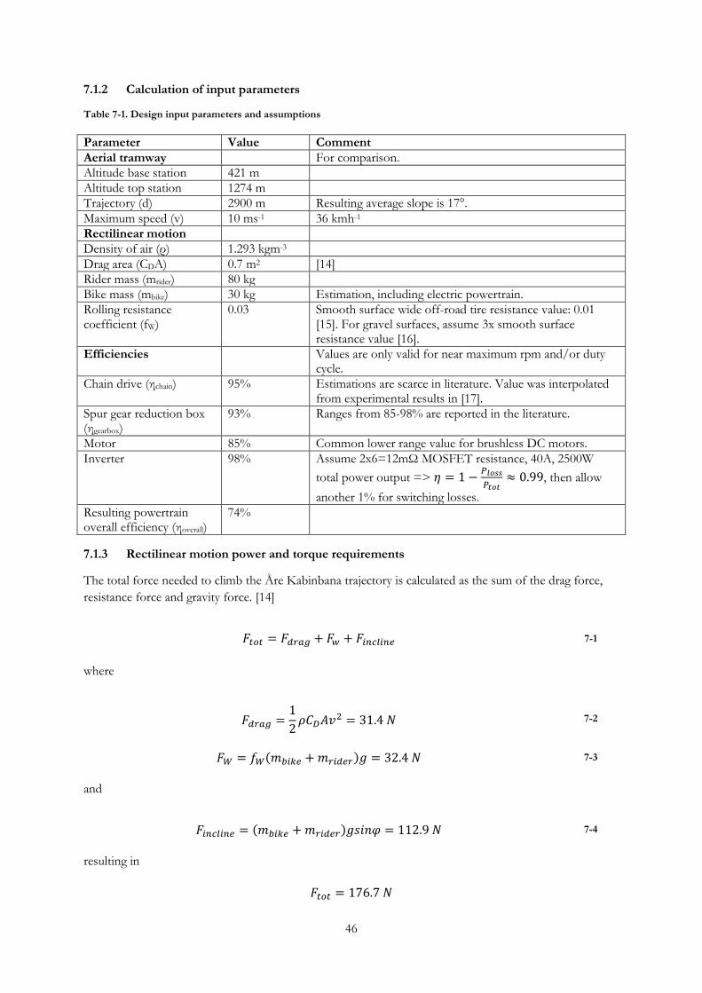
46
7.1.2 Calculation of input parameters
Table 7-1. Design input parameters and assumptions
Parameter Value Comment
Aerial tramway For comparison.
Altitude base station 421 m
Altitude top station 1274 m
Trajectory (d) 2900 m Resulting average slope is 17°.
Maximum speed (v) 10 ms-1 36 kmh-1
Rectilinear motion
Density of air (ρ) 1.293 kgm-3
Drag area (CDA) 0.7 m2 [14]
Rider mass (mrider) 80 kg
Bike mass (mbike) 30 kg Estimation, including electric powertrain.
Rolling resistance coefficient (fW)
0.03 Smooth surface wide off-road tire resistance value: 0.01 [15]. For gravel surfaces, assume 3x smooth surface resistance value [16].
Efficiencies Values are only valid for near maximum rpm and/or duty cycle.
Chain drive (ηchain) 95% Estimations are scarce in literature. Value was interpolated from experimental results in [17].
Spur gear reduction box (ηgearbox)
93% Ranges from 85-98% are reported in the literature.
Motor 85% Common lower range value for brushless DC motors.
Inverter 98% Assume 2x6=12mΩ MOSFET resistance, 40A, 2500W
total power output =>
, then allow
another 1% for switching losses.
Resulting powertrain overall efficiency (ηoverall)
74%
7.1.3 Rectilinear motion power and torque requirements
The total force needed to climb the Åre Kabinbana trajectory is calculated as the sum of the drag force,
resistance force and gravity force. [14]
7-1
where
7-2
( ) 7-3
and
( ) 7-4
resulting in
47
The resulting nominal power requirement at the wheel at vbike is
7-5
Adjusted for efficiency, the dimensioning power requirement is
7-6
7.1.3.1 Rectilinear speed requirement
The DH rider cannot always count on the forces of gravity, and the maximum velocity attainable during
short spurts of high cadence pedaling at top gear is
7-7
which leaves the vbike speed as dimensioning. This corresponds to a rear wheel angular speed of 25.3 rad s-
1 or 241.4 rpm(30).
7.1.3.2 Resulting motor torque requirement
The torque requirement about the drive wheel is calculated to be
7-8
Back-calculating from wheel torque requirement, the motor torque requirement can be stated as
7-9
where ngear is the chosen gear ratio.
7.1.4 Single load cycle equivalent battery mass requirement
The energy used in the downhill part of a single uphill-down load cycle is negligible compared to that of
the uphill cycle, which is
7-10
A possible building block battery for these purposes is the eight cell generic R/C 5.8 Ah lithium polymer
battery, with a nominal voltage of 30.4 V and a mass of 1.3 kg. This battery contains approximately
30 The DH bike has a 26” wheel with a circumference of approximately 2.07 m.

48
7-11
of energy and the number of such batteries ideally needed for one single load cycle is
7-12
In the course of this thesis work, as a design constraint, it is assumed that the power source consists of
two such batteries connected in series, resulting in a 60.8 V nominal system voltage, and a total battery
system mass of 2.8 kg.

49
7.2 Appendix B: Experimental setup and test bike
7.2.1 Experimental setup
A low-power and failure friendly development setup was created in order to gain a general understanding
of the drive and to enable ballpark tuning of hardware and software before creation of the final inverter-
controller.
Figure 7-2. Block diagram presentation of experimental setup. Solid lines represent power flows, dashed lines are signals.
7.2.1.1 DC-source
Generic 12 V/7.2 Ah lead acid batteries connected in series to produce a 12-48 VDC output.
7.2.1.2 VSI and DSP
The simple controller-inverter setup is a combination of breadboard and PCB based electronics. Signal
electronics, such as the DSP, supply voltage transformation and gate drivers were implemented on
breadboard, whereas power electronic components were soldered to a PCB. Key components are listed in
the table below. Where possible, the same components are used that are projected for the final controller
inverter.
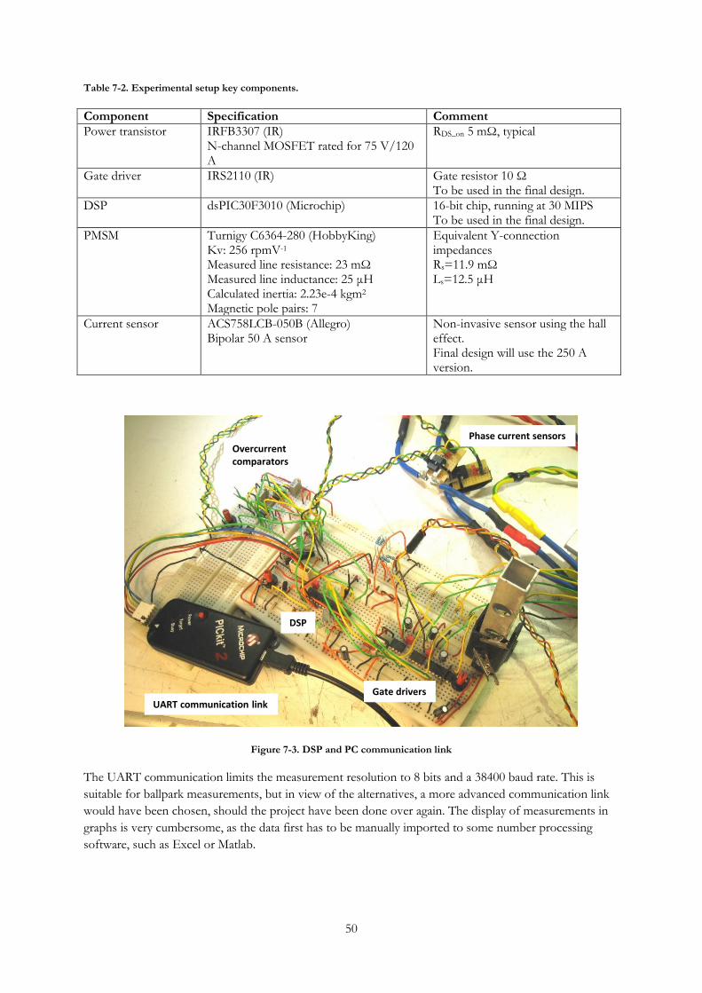
50
Table 7-2. Experimental setup key components.
Component Specification Comment
Power transistor IRFB3307 (IR) N-channel MOSFET rated for 75 V/120 A
RDS_on 5 mΩ, typical
Gate driver IRS2110 (IR) Gate resistor 10 Ω To be used in the final design.
DSP dsPIC30F3010 (Microchip) 16-bit chip, running at 30 MIPS To be used in the final design.
PMSM Turnigy C6364-280 (HobbyKing) Kv: 256 rpmV-1
Measured line resistance: 23 mΩ Measured line inductance: 25 μH Calculated inertia: 2.23e-4 kgm2
Magnetic pole pairs: 7
Equivalent Y-connection impedances Rs=11.9 mΩ Ls=12.5 μH
Current sensor ACS758LCB-050B (Allegro) Bipolar 50 A sensor
Non-invasive sensor using the hall effect. Final design will use the 250 A version.
Figure 7-3. DSP and PC communication link
The UART communication limits the measurement resolution to 8 bits and a 38400 baud rate. This is
suitable for ballpark measurements, but in view of the alternatives, a more advanced communication link
would have been chosen, should the project have been done over again. The display of measurements in
graphs is very cumbersome, as the data first has to be manually imported to some number processing
software, such as Excel or Matlab.
Gate drivers
DSP
Phase current sensorsOvercurrent comparators
UART communication link
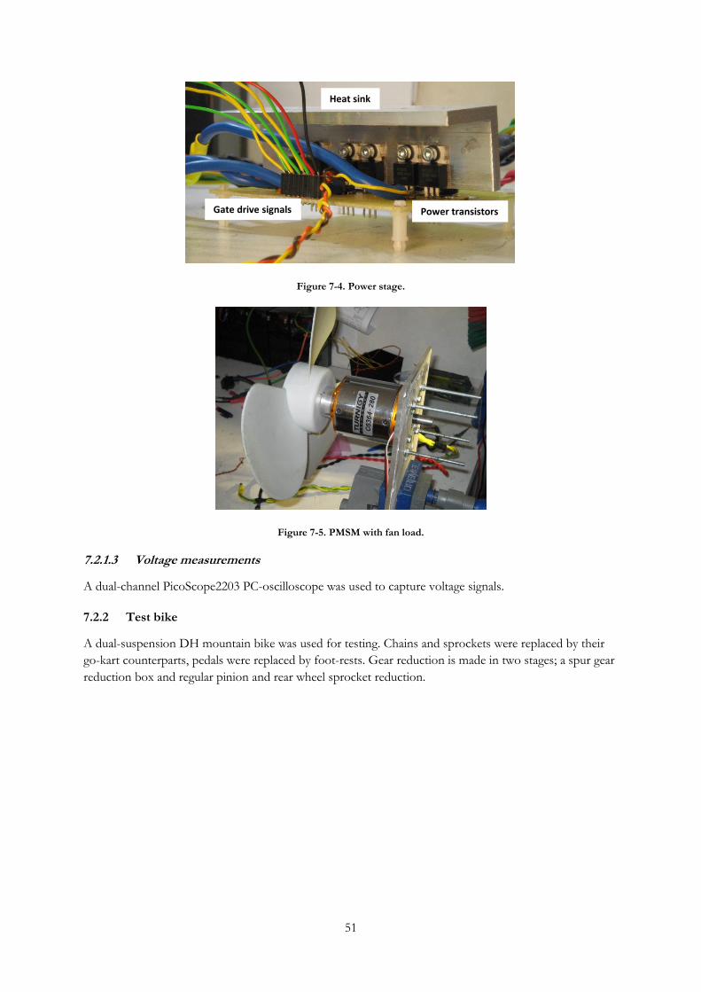
51
Figure 7-4. Power stage.
Figure 7-5. PMSM with fan load.
7.2.1.3 Voltage measurements
A dual-channel PicoScope2203 PC-oscilloscope was used to capture voltage signals.
7.2.2 Test bike
A dual-suspension DH mountain bike was used for testing. Chains and sprockets were replaced by their
go-kart counterparts, pedals were replaced by foot-rests. Gear reduction is made in two stages; a spur gear
reduction box and regular pinion and rear wheel sprocket reduction.
Heat sink
Power transistorsGate drive signals
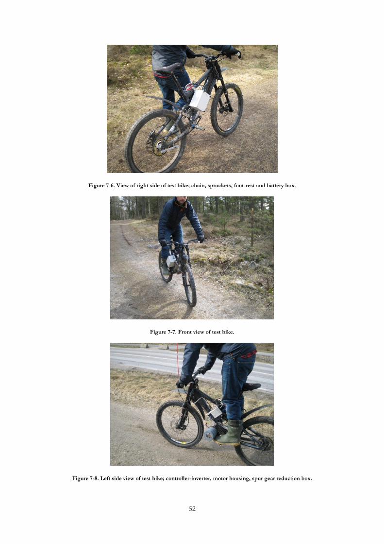
52
Figure 7-6. View of right side of test bike; chain, sprockets, foot-rest and battery box.
Figure 7-7. Front view of test bike.
Figure 7-8. Left side view of test bike; controller-inverter, motor housing, spur gear reduction box.
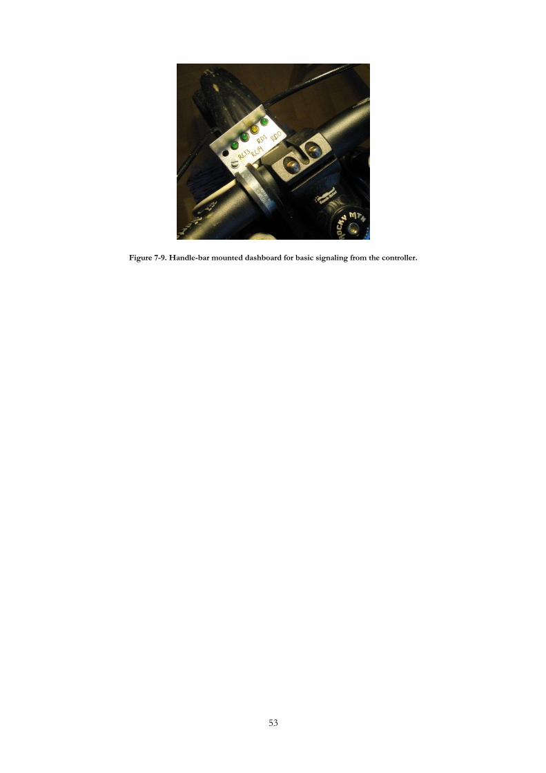
53
Figure 7-9. Handle-bar mounted dashboard for basic signaling from the controller.


55
7.3 Appendix C: Per unit model % Turnigy 80/100-130 parameters and pu derivation % RMS=1/sqrt(2); Rds_on=5e-3; Kv=118; Rs_delta=19.6e-3; Ls_delta=38.5e-6; p=7; % Pole-pairs Kt=1/Kv*60/(2*pi); lamaf=Kt*2/(3*p); % Rotor magnetic flux
% Y-equivalents Rs=Rs_delta/2+Rds_on; Ls=Ls_delta/2;
% pu model DClink=16*3.8; % Number of cells * Lipo nominal cell voltage Imotor_rated=80; % Rated motor current lamb=lamaf; % Base flux linkages Vb3=DClink*RMS; % Rated phase voltage Vb=1/RMS*Vb3; % dq-frame base voltage Ib=Imotor_rated; % dq-frame base current Zb=Vb/Ib; % Base impedance w_b=Vb/lamb; % Base electrical speed Lb=Zb/w_b; % Base inductance Rsn=Rs/Zb; % Normalized stator resistance Lsn=Ls/Lb; % Normalized stator inductance Tb=3/2*p*lamb*Ib; % Base torque
% Overall drive parameters gearing=12.7; w_wheel=30.35*1.1; % Target speed in rad/s, with 10% slip margin w_target_en=w_wheel*gearing*7/w_b; % Corresponding electrical rotor speed
Related Documents