CONFIDENCE IN THE CONFIDENCE FACTOR

CONFIDENCE IN THE CONFIDENCE FACTOR

Paolo Franchin a, Paolo Emilio Pinto a Pathmanathan Rajeev b

a Dept. of Structural Engineering & Geotechnics, Sapienza University of Rome, Rome, Italy, { paolo.franchin,pinto}@uniroma1.it

b European School for Advanced Studies in Seismic Risk, Pavia, Italy [email protected]

ABSTRACT EC8-3, devoted to assessment/retrofitting of existing buildings, accounts for epistemic uncertainty with an adjustment factor, called “confidence factor (CF)”, whose value depends on the knowledge of properties such as geometry, reinforcement layout and detailing, and materials. This solution, plausible from a logical point of view, cannot yet profit from the experience of use in practice, hence it needs to be substantiated by a higher level probabilistic analysis accounting for and propagating epistemic uncertainty (i.e., incomplete knowledge of a structure) throughout the seismic assessment procedure. The paper investigates the soundness of the proposed format and pinpoints some problematic aspects that would require refinement. The approach taken rests on the simulation of the entire assessment procedure and the evaluation the distribution of the assessment results conditional on the acquired knowledge. Based on this distribution a criterion is proposed to calibrate the CF values. The obtained values are then critically examined and compared with code-specified ones.

KEYWORDS Reinforced concrete, Testing and Inspection, Reinforcement details, Material properties, Modelling assumptions, Analysis method, Knowledge level.

1 CURRENT RESEARCH AND NORMATIVE GAP

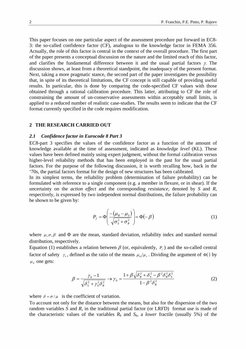
The obvious fact that the major proportion of seismic risk, in terms of human lives and economic loss, is posed to the society from existing structures is a surprisingly recent acquisition. It took a few disastrous events in California and Japan in the ‘90s to make the vastness of the problem apparent, and to expose the unpreparedness of the scientific-technical community. Research and code-writing in particular had been occupied with progressing the state-of-the-art in the design of new, well-behaving structures, a task much simpler than the assessment of existing, defective ones. In this vacuum the first document aligned with the modern anti-seismic philosophy can be considered to be the NEHRP guidelines, prepared in 1997 under the sponsorship of the FEMA (FEMA, 1997), followed in 2000 by the FEMA 356 (FEMA, 2000). In the same years work started on Eurocode 8 Part 3 which was finally approved in 2005 (CEN, 2005). Of course, it could not be asked of these documents to provide a knowledge that did not exist and, given the relatively short period during which they were developed, it could also not be expected that they were validated through a sufficiently long experience of application. As a result, they should still be looked at as experimental and subject to further progress.

P. Franchin, P.E. Pinto, P. Rajeev

2

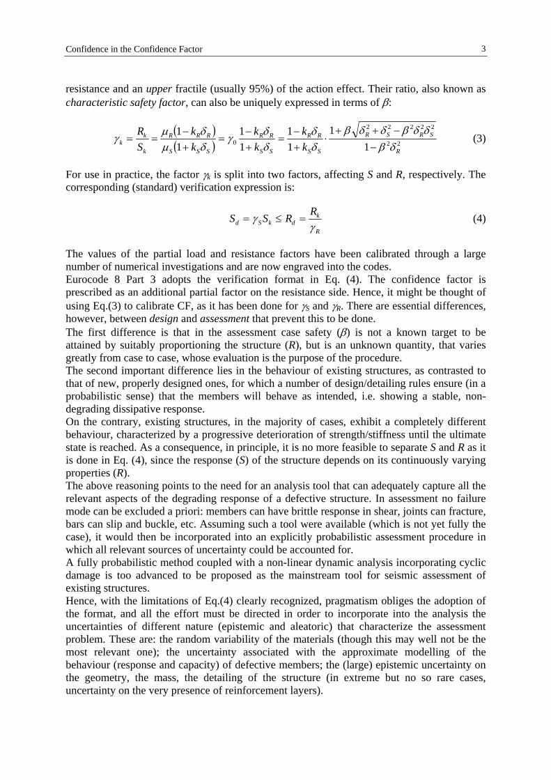
This paper focuses on one particular aspect of the assessment procedure put forward in EC8-3: the so-called confidence factor (CF), analogous to the knowledge factor in FEMA 356. Actually, the role of this factor is central in the context of the overall procedure. The first part of the paper presents a conceptual discussion on the nature and the limited reach of this factor, and clarifies the fundamental difference between it and the usual partial factors γ. The discussion shows, at least from a theoretical standpoint, the inadequacy of the present format. Next, taking a more pragmatic stance, the second part of the paper investigates the possibility that, in spite of its theoretical limitations, the CF concept is still capable of providing useful results. In particular, this is done by comparing the code-specified CF values with those obtained through a rational calibration procedure. This latter, attributing to CF the role of constraining the amount of un-conservative assessments within acceptably small limits, is applied to a reduced number of realistic case-studies. The results seem to indicate that the CF format currently specified in the code requires modification.

2 THE RESEARCH CARRIED OUT

2.1 Confidence factor in Eurocode 8 Part 3 EC8-part 3 specifies the values of the confidence factor as a function of the amount of knowledge available at the time of assessment, indicated as knowledge level (KL). These values have been defined mainly using expert judgment, without the formal calibration versus higher-level reliability methods that has been employed in the past for the usual partial factors. For the purpose of the following discussion, it is worth recalling how, back in the ‘70s, the partial factors format for the design of new structures has been calibrated. In its simplest terms, the reliability problem (determination of failure probability) can be formulated with reference to a single component (e.g. a member in flexure, or in shear). If the uncertainty on the action effect and the corresponding resistance, denoted by S and R, respectively, is expressed by two independent normal distributions, the failure probability can be shown to be given by:

( ) ( )βσσµµ

−Φ=⎟⎟

⎠

⎞

⎜⎜

⎝

⎛

+

−−Φ=

22RS

SRfP (1)

where βσµ , , and Φ are the mean, standard deviation, reliability index and standard normal distribution, respectively. Equation (1) establishes a relation between β (or, equivalently, fP ) and the so-called central factor of safety 0γ , defined as the ratio of the means SR µµ . Dividing the argument of ( )⋅Φ by

Sµ one gets:

22

22222

0220

2

0

111

R

SRSR

RSδβ

δδβδδβγ

δγδ

γβ

−

−++=→

+

−= (2)

where µσδ /= is the coefficient of variation. To account not only for the distance between the means, but also for the dispersion of the two random variables S and R, in the traditional partial factor (or LRFD) format use is made of the characteristic values of the variables Rk and Sk, a lower fractile (usually 5%) of the

Confidence in the Confidence Factor

3

resistance and an upper fractile (usually 95%) of the action effect. Their ratio, also known as characteristic safety factor, can also be uniquely expressed in terms of β:

( )( ) 22

22222

0 11

11

11

11

R

SRSR

SS

RR

SS

RR

SSS

RRR

k

kk k

kkk

kk

SR

δβδδβδδβ

δδ

δδγ

δµδµγ

−−++

⋅+−

=+−

=+−

== (3)

For use in practice, the factor γk is split into two factors, affecting S and R, respectively. The corresponding (standard) verification expression is:

R

kdkSd

RRSSγ

γ =≤= (4)

The values of the partial load and resistance factors have been calibrated through a large number of numerical investigations and are now engraved into the codes. Eurocode 8 Part 3 adopts the verification format in Eq. (4). The confidence factor is prescribed as an additional partial factor on the resistance side. Hence, it might be thought of using Eq.(3) to calibrate CF, as it has been done for γS and γR. There are essential differences, however, between design and assessment that prevent this to be done. The first difference is that in the assessment case safety (β) is not a known target to be attained by suitably proportioning the structure (R), but is an unknown quantity, that varies greatly from case to case, whose evaluation is the purpose of the procedure. The second important difference lies in the behaviour of existing structures, as contrasted to that of new, properly designed ones, for which a number of design/detailing rules ensure (in a probabilistic sense) that the members will behave as intended, i.e. showing a stable, non-degrading dissipative response. On the contrary, existing structures, in the majority of cases, exhibit a completely different behaviour, characterized by a progressive deterioration of strength/stiffness until the ultimate state is reached. As a consequence, in principle, it is no more feasible to separate S and R as it is done in Eq. (4), since the response (S) of the structure depends on its continuously varying properties (R). The above reasoning points to the need for an analysis tool that can adequately capture all the relevant aspects of the degrading response of a defective structure. In assessment no failure mode can be excluded a priori: members can have brittle response in shear, joints can fracture, bars can slip and buckle, etc. Assuming such a tool were available (which is not yet fully the case), it would then be incorporated into an explicitly probabilistic assessment procedure in which all relevant sources of uncertainty could be accounted for. A fully probabilistic method coupled with a non-linear dynamic analysis incorporating cyclic damage is too advanced to be proposed as the mainstream tool for seismic assessment of existing structures. Hence, with the limitations of Eq.(4) clearly recognized, pragmatism obliges the adoption of the format, and all the effort must be directed in order to incorporate into the analysis the uncertainties of different nature (epistemic and aleatoric) that characterize the assessment problem. These are: the random variability of the materials (though this may well not be the most relevant one); the uncertainty associated with the approximate modelling of the behaviour (response and capacity) of defective members; the (large) epistemic uncertainty on the geometry, the mass, the detailing of the structure (in extreme but no so rare cases, uncertainty on the very presence of reinforcement layers).


4

The described sources of uncertainty may lead different analysts to widely different results on the same structure to be assessed. This is illustrated in some detail in the next section.

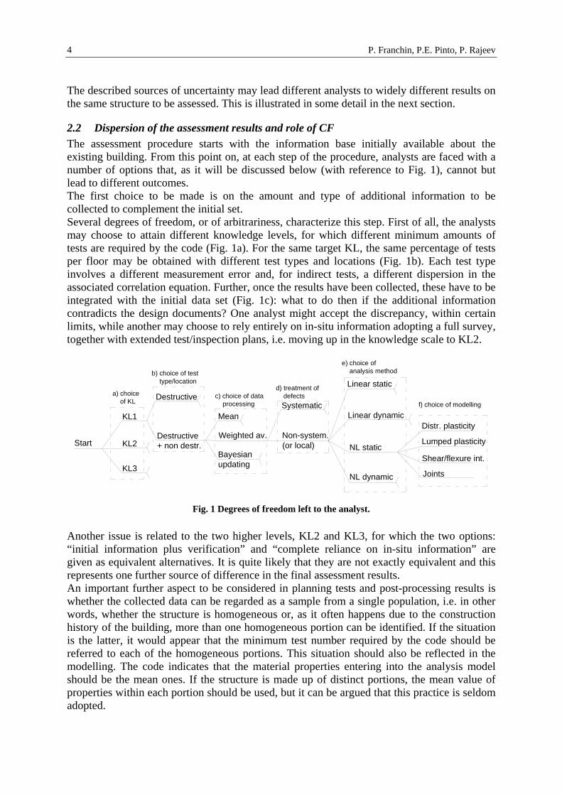
2.2 Dispersion of the assessment results and role of CF The assessment procedure starts with the information base initially available about the existing building. From this point on, at each step of the procedure, analysts are faced with a number of options that, as it will be discussed below (with reference to Fig. 1), cannot but lead to different outcomes. The first choice to be made is on the amount and type of additional information to be collected to complement the initial set. Several degrees of freedom, or of arbitrariness, characterize this step. First of all, the analysts may choose to attain different knowledge levels, for which different minimum amounts of tests are required by the code (Fig. 1a). For the same target KL, the same percentage of tests per floor may be obtained with different test types and locations (Fig. 1b). Each test type involves a different measurement error and, for indirect tests, a different dispersion in the associated correlation equation. Further, once the results have been collected, these have to be integrated with the initial data set (Fig. 1c): what to do then if the additional information contradicts the design documents? One analyst might accept the discrepancy, within certain limits, while another may choose to rely entirely on in-situ information adopting a full survey, together with extended test/inspection plans, i.e. moving up in the knowledge scale to KL2.

KL1

Destructive

Destructive+ non destr.KL2

KL3

Mean

Weighted av.

Bayesianupdating

a) choice of KL

b) choice of test type/location

c) choice of data processing

Non-system.(or local)

Systematic

d) treatment of defects

Linear static

Linear dynamic

NL static

NL dynamic

Start

e) choice of analysis method

f) choice of modelling

Distr. plasticity

Lumped plasticity

Shear/flexure int.

Joints

Fig. 1 Degrees of freedom left to the analyst.

Another issue is related to the two higher levels, KL2 and KL3, for which the two options: “initial information plus verification” and “complete reliance on in-situ information” are given as equivalent alternatives. It is quite likely that they are not exactly equivalent and this represents one further source of difference in the final assessment results. An important further aspect to be considered in planning tests and post-processing results is whether the collected data can be regarded as a sample from a single population, i.e. in other words, whether the structure is homogeneous or, as it often happens due to the construction history of the building, more than one homogeneous portion can be identified. If the situation is the latter, it would appear that the minimum test number required by the code should be referred to each of the homogeneous portions. This situation should also be reflected in the modelling. The code indicates that the material properties entering into the analysis model should be the mean ones. If the structure is made up of distinct portions, the mean value of properties within each portion should be used, but it can be argued that this practice is seldom adopted.


5

For all of the considerations above, already at the end of this first step (data collection and processing) every analyst will have a different picture of the same structure. The next branching point has to do with the so-called defective details, such as, for example, insufficient anchorage length of rebars, 90° hooks and inadequate diameter/spacing in stirrups, absence of joint reinforcement or wrong detailing of the anchorage of longitudinal bars into the joint, etc. This is a multi-faceted problem. Once a type of defect is discovered, the question arises whether its presence should be considered systematic over the structure or a portion of it only, or as an isolated local feature (Fig. 1d). An informed answer to this question would require extensive and intrusive investigations that are seldom compatible with the continued use of a building. The next choice of the analysts is the method of analysis to be employed (Fig. 1e), which is intimately related to that of the modelling (Fig. 1f). Obviously, if the selected analysis is linear, the cyclic degradation due to defects cannot be included at this stage. But even if it is nonlinear static, such behaviour cannot be easily included. Exclusion of these defects from modelling may lead to a response (S) quite different from the real one, which would then be compared to a resistance (R) affected by large uncertainty (model uncertainty on the capacity formulas for defective members). On the other hand, nonlinear dynamic analysis including behavioural models for defective members would trade the model uncertainty on capacity with that on hysteretic degrading response. The different sources of uncertainty and multiple choices facing the analysts during the assessment, all contribute to a relatively large dispersion in the estimated state of the structure. The above discussion makes it overwhelmingly clear that the nature of the confidence factor is different from that of the partial factors recalled in Section 1. The interpretation that is proposed herein for the CF is that of a factor which aims at ensuring that, out of a large number of assessments carried out in accordance with EC8-3, only a predefined, acceptably small fraction of them leads to an unsafe result, i.e. to overestimating the actual safety. Admittedly, the idea that a single factor, with values depending only on the knowledge level, and not on all the aspects recalled above, may achieve the stated objective may appear as unrealistic. The paper represents an attempt to investigate to what extent this idea maintains some value. Further it provides a limited exploration on the magnitude of the CF values needed to reach the stated goal.

2.3 Proposed procedure for the evaluation of CF values The proposed procedure consists of a simulation of the entire EC8-3 assessment process with the purpose of quantifying the dispersion in the assessment results due to the many choices/uncertainties described in the previous section. The starting point of the procedure is to imagine an existing building, with all its properties, including the defects and spatial fluctuation of materials, geometry, etc. completely known. This ideal state of perfect knowledge can never be obtained in practice and it represents a state of knowledge higher (the highest possible) than the state of so-called complete knowledge described in the code (KL3). In each simulation run choices (knowledge level, type and position of tests, how to process the results, analysis method, modelling options, etc) are made randomly to reflect the arbitrary choices made by different analysts. This obviously requires the spelling-out of all the steps described in the previous section, discretizing the possible choices in a finite number of options and filling the gaps of the code with practices coming from common-sense and experience in real-case assessments. It is imagined that the generic analyst will follow his trail


6

down the procedure arriving at a different evaluation of the safety of the structure. This simulation is carried out without employing the confidence factor (i.e. CF=1). By repeating the process for a sufficiently large number, say n, of analysts a statistical sample (of size n) of the structural safety is obtained and can be used to estimate its distribution. At this stage the statistical sample of structural states, quantified by the global state variable Y (a critical demand to capacity ratio, see Jalayer et al 2007) is compared with the true state of the structure, i.e. the state of the structure evaluated based on the ideal perfect state of knowledge. It is expected that a portion of the assessments will result in a conservative estimate (i.e. in a state worst than the real one) while the remaining will be on the un-conservative side. The goal of the last part of the procedure is that of reducing the fraction of un-conservative estimates to an acceptably small value. This is done by re-evaluating the structural state, using the same sets of choices of the previous evaluation, with a value of CF larger than one (i.e. decreasing capacities). If the procedure works as intended the new sample of structural states will have the predefined target fraction of un-conservative estimates. The procedure can be split into the following steps: • Step 1: Generation of the existing and perfectly known structure (termed reference

structure) Once all the material properties and possible defects have been assigned a probability distribution, a structure can be generated by sampling a set of parameter values from the above distributions. This structure is by definition completely known and is termed the reference structure.

• Step 2: Generation of a sample of imperfectly-known structures from the reference structure A number NVA of virtual analysts is given the task of assessing the structure. This step consists of simulating the process of inspection/information-collection, and produces NVA different states of (imperfect) knowledge from the reference structure. These states are the starting point for the assessment by the virtual analysts. In order to reflect the different test plans designed by different analysts, this step requires the randomization of the test locations and test types.

• Step 3: Assessment of the reference structure The reference structure is assessed according to the code and the seismic intensity that induces the attainment of the limit-state (LS) under consideration is recorded. The attainment of the limit state is marked by a unit value of the global variable Y=1. This result is considered the true state of the structure.

• Step 4: Assessment of the imperfectly known structures The virtual analysts apply the code-based assessment procedure with a unit value of the CF and the same intensity as determined in Step 3. This produces a sample of NVA values of the global state variable Y. This step requires a further randomization, reflecting the freedom left to the code-user in choices such as inclusion/exclusion of defects from modelling and the selection of the analysis method (linear vs. nonlinear, static vs. dynamic).

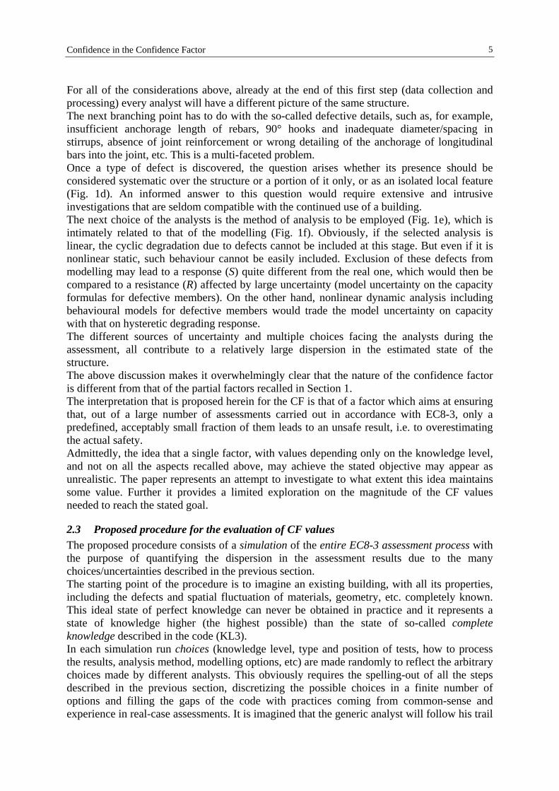
• Step 5: Statistical processing of the sample states and determination of CF Statistical processing of the sample of values of Y produces a distribution that exhibits a certain amount of variability around the value Y=1. This is shown in Fig. 2a. The value of the CF can now be determined by enforcing the condition that a chosen lower fractile of Y (say, 10%) is equal to 1, i.e. the true state of the structure (as shown in Fig. 2b).


7

YY*=1

0.5

1.0

F(Y|KL)

(a)

YY*=1

0.5

1.0

F(Y|KL)

(b)

0.1

CF>1

YY*=1

0.5

1.0

F(Y|KL)

(a)

YY*=1

0.5

1.0

F(Y|KL)

(b)

0.1

CF>1

Fig. 2 Distribution of the assessment results made by the NVA analysts: a) with CF = 1, b) with CF>1.

2.4 Application to three RC plane frame structures

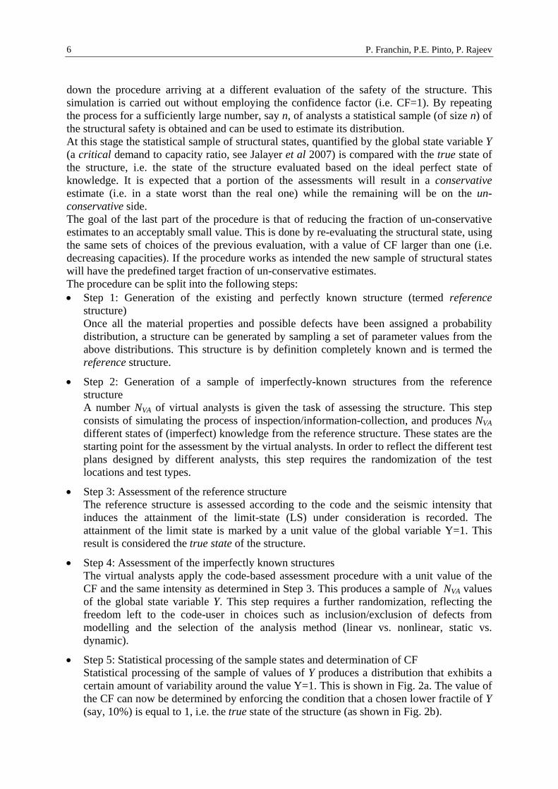
2.4.1 Geometry and modelling of the structures The calibration procedure has been applied to three RC frame structures selected in order of increasing “complexity” (Fig. 3). They have been selected to investigate whether CF values, which according to the proposal are a function of the distribution (spread) of structural response, are sufficiently stable with increasing structural size.

(A)Two-storey, three-bay

symmetric frame

(B)Five-storey, four-bay

symmetric frame

(C)Six-storey, three-bay non

symmetric frame

(A)Two-storey, three-bay

symmetric frame

(B)Five-storey, four-bay

symmetric frame

(C)Six-storey, three-bay non

symmetric frame

Fig. 3 The analyzed structures.

For the purpose of data collection (material tests, reinforcement details etc.) and post-processing the structures are considered homogenous, in the sense that the spatial distribution of the properties/defects belongs to a single population. The assessment has been carried out with the nonlinear static and dynamic methods. CF values have been evaluated both separately with each of the two methods, and jointly, to investigate dependence on the analysis method. For the purpose of dynamic analysis the seismic action is represented by seven recorded ground motions selected to fit on average, with minimum scaling, the EC8-specified spectral shape scaled to a PGA of 0.35g for soil class A (Iervolino et al, 2008). In the case of static analysis, the average spectrum of the recorded ground motions is considered as the demand spectrum. In terms of modelling the nonlinear degrading response of the structure, account has been taken of flexure-shear interaction and joint hysteretic response. The models are set up in OpenSEES, employing flexibility-based elements for the members with section aggregator to


8

couple a fibre section (flexural response) with a degrading hysteretic shear force-deformation law. Joints have been modelled with a “scissor-model” with a degrading hysteretic shear force-deformation law. Tangent-stiffness proportional damping has been used, calibrated to yield a 5% equivalent viscous damping ratio on the first elastic mode. Since the effect of brittle failure modes, such as shear in members and joints, has been included in the modelling (for both static and dynamic analysis), the structural performance is checked in terms of deformation quantities only. Hence, CY θθmax= , where θmax is the demand peak inter-storey drift ratio, and θC the corresponding capacity. Detailed information on the characteristics (geometry, reinforcement, etc) of the structures and the adopted response models can be found in (Rajeev, 2008).

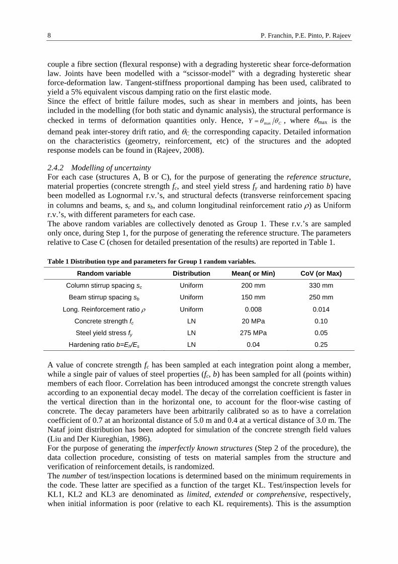
2.4.2 Modelling of uncertainty For each case (structures A, B or C), for the purpose of generating the reference structure, material properties (concrete strength fc, and steel yield stress fy and hardening ratio b) have been modelled as Lognormal r.v.’s, and structural defects (transverse reinforcement spacing in columns and beams, sc and sb, and column longitudinal reinforcement ratio ρ) as Uniform r.v.’s, with different parameters for each case. The above random variables are collectively denoted as Group 1. These r.v.’s are sampled only once, during Step 1, for the purpose of generating the reference structure. The parameters relative to Case C (chosen for detailed presentation of the results) are reported in Table 1.

Table 1 Distribution type and parameters for Group 1 random variables.

Random variable Distribution Mean( or Min) CoV (or Max)

Column stirrup spacing sc Uniform 200 mm 330 mm

Beam stirrup spacing sb Uniform 150 mm 250 mm

Long. Reinforcement ratio ρ Uniform 0.008 0.014

Concrete strength fc LN 20 MPa 0.10

Steel yield stress fy LN 275 MPa 0.05

Hardening ratio b=Eh/Es LN 0.04 0.25

A value of concrete strength fc has been sampled at each integration point along a member, while a single pair of values of steel properties (fc, b) has been sampled for all (points within) members of each floor. Correlation has been introduced amongst the concrete strength values according to an exponential decay model. The decay of the correlation coefficient is faster in the vertical direction than in the horizontal one, to account for the floor-wise casting of concrete. The decay parameters have been arbitrarily calibrated so as to have a correlation coefficient of 0.7 at an horizontal distance of 5.0 m and 0.4 at a vertical distance of 3.0 m. The Nataf joint distribution has been adopted for simulation of the concrete strength field values (Liu and Der Kiureghian, 1986). For the purpose of generating the imperfectly known structures (Step 2 of the procedure), the data collection procedure, consisting of tests on material samples from the structure and verification of reinforcement details, is randomized. The number of test/inspection locations is determined based on the minimum requirements in the code. These latter are specified as a function of the target KL. Test/inspection levels for KL1, KL2 and KL3 are denominated as limited, extended or comprehensive, respectively, when initial information is poor (relative to each KL requirements). This is the assumption


9

made herein. The actual number of tests together with the code minima for structure c are reported in Table 2. The number of tests results always slightly larger than the minimum, with only one (negligible) exception. The actual test location chosen by each analyst is determined by randomly sampling (uniform integer distribution) first the member and then the location within the member (for this purpose each integration point is regarded as a possible test location). At each location, the testing/inspection consists of reading the value of the sought property from the reference structure (value generated during Step 1). Measurement errors are not considered. Since the reference structure is homogeneous by assumption, all the data gathered are averaged to obtain the values to be employed in the assessment.

Table 2 Number of test/inspections (minima for construction details are meant per element type: columns, beams).

KL Testing (material) Inspection (details)

Minimum Actual Minimum Actual

1 Limited 1 per floor 1 per floor (6) 20% 1 × floor × type, 6/24 col.’s = 25%, 6/18 beams = 33%

2 Extended 2 per floor 2 per floor (12) 50% 2 × floor × type, 12/24 col.’s = 50%, 12/18 beams = 66%

3 Comprehensive 3 per floor 3 per floor (18) 80% 3 × floor × type, 18/24 col.’s = 75%, 18/18 beams = 100%

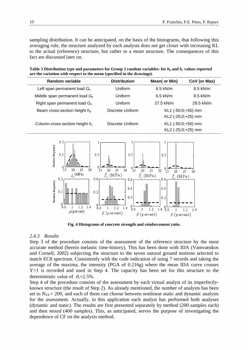
The assumed scarceness of initial information, and in particular the lack of a complete set of construction drawings, influences the knowledge of the geometry of the structure. In particular, this may refer to the presence/absence of elements (a typical case being represented by beams in flat-slab structures) or the actual cross-section dimensions (significant variations in plaster thickness or the presence of cavities for ducts are common and cannot practically be ascertained for all members), or, finally, the precise unit-area weight of the floor system. To model this kind of “geometrical” uncertainties (denoted as “residual” in the following) two types of additional random variables are introduced: the unit-area weight of floors (one variable per floor typology, e.g. typical floor and roof) and the cross section height of elements (one variable per element type: beams and columns). These random variables are collectively denoted as Group 2 and are sampled for each imperfectly known structure during Step 2. Table 3 shows the corresponding distribution types and parameters for case C. To illustrate Steps 1 and 2, Fig. 4 shows for Structure C the histograms of the relative frequency of a number of quantities. The leftmost column reports the histograms of the concrete strength fc and of the columns’ reinforcement ratio ρ for the reference structure, chosen to represent material properties and construction details, respectively. The plots show also the original distribution from which the values have been sampled (see Table 1). The sample size is 162 (one value per integration point, 24 columns with 3 points each, 18 beams with 5 points each) and 24 (one value per column), respectively. The following three columns report for the three KLs the histograms of the values cf and ρ obtained averaging the test results by each analyst (hence the sample size for both quantities equals the number NVA = 200 of virtual analysts). The average values cf and ρ are obtained from samples of size increasing with KL: for instance, 6, 12 or 18 fc values for KL1, 2 and 3. Clearly a larger sample leads to an estimate of the mean closer to the true mean. This latter, of course, is the mean of the values sampled for the reference structure, not the mean of the


10

sampling distribution. It can be anticipated, on the basis of the histograms, that following this averaging rule, the structure analyzed by each analysts does not get closer with increasing KL to the actual (reference) structure, but rather to a mean structure. The consequences of this fact are discussed later on.

Table 3 Distribution type and parameters for Group 2 random variables: for hb and hc values reported are the variation with respect to the mean (specified in the drawings).

Random variable Distribution Mean( or Min) CoV (or Max)

Left span permanent load Gk Uniform 6.5 kN/m 8.5 kN/m

Middle span permanent load Gk Uniform 6.5 kN/m 8.5 kN/m

Right span permanent load Gk Uniform 27.5 kN/m 29.5 kN/m

Beam cross-section height hb Discrete Uniform KL1 (-50;0;+50) mm KL2 (-25;0;+25) mm

Column cross-section height hc Discrete Uniform KL1 (-50;0;+50) mm KL2 (-25;0;+25) mm

Fig. 4 Histograms of concrete strength and reinforcement ratio.

2.4.3 Results Step 3 of the procedure consists of the assessment of the reference structure by the most accurate method (herein inelastic time-history). This has been done with IDA (Vamvatsikos and Cornell, 2002) subjecting the structure to the seven natural ground motions selected to match EC8 spectrum. Consistently with the code indication of using 7 records and taking the average of the maxima, the intensity (PGA of 0.216g) where the mean IDA curve crosses Y=1 is recorded and used in Step 4. The capacity has been set for this structure to the deterministic value of θc=2.5%. Step 4 of the procedure consists of the assessment by each virtual analyst of its imperfectly-known structure (the result of Step 2). As already mentioned, the number of analysts has been set to NVA = 200, and each of them can choose between nonlinear static and dynamic analysis for the assessment. Actually, in this application each analyst has performed both analyses (dynamic and static). The results are first presented separately by method (200 samples each) and then mixed (400 samples). This, as anticipated, serves the purpose of investigating the dependence of CF on the analysis method.


11

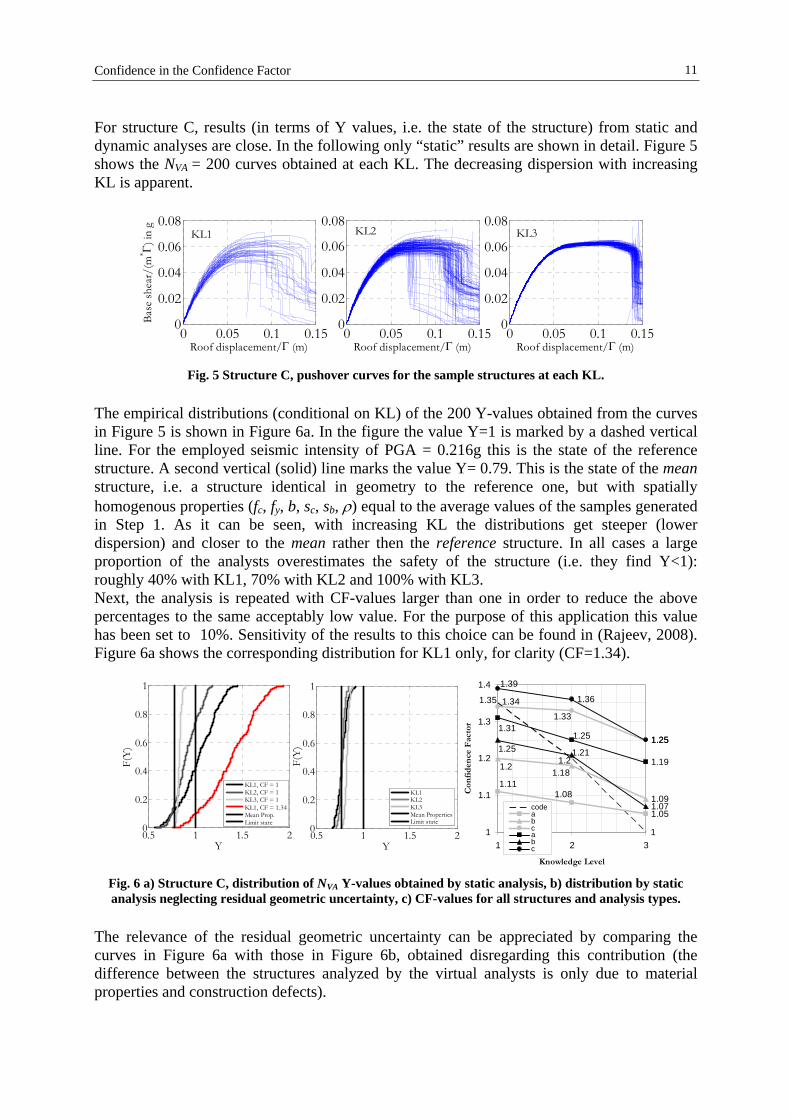
For structure C, results (in terms of Y values, i.e. the state of the structure) from static and dynamic analyses are close. In the following only “static” results are shown in detail. Figure 5 shows the NVA = 200 curves obtained at each KL. The decreasing dispersion with increasing KL is apparent.

0 0.05 0.1 0.150

0.02

0.04

0.06

0.08

Roof displacement/Γ (m)

Base

shea

r/(m

* Γ) i

n g

KL1 KL1

0 0.05 0.1 0.150

0.02

0.04

0.06

0.08


KL2

0 0.05 0.1 0.150

0.02

0.04

0.06

0.08


KL3

Fig. 5 Structure C, pushover curves for the sample structures at each KL.

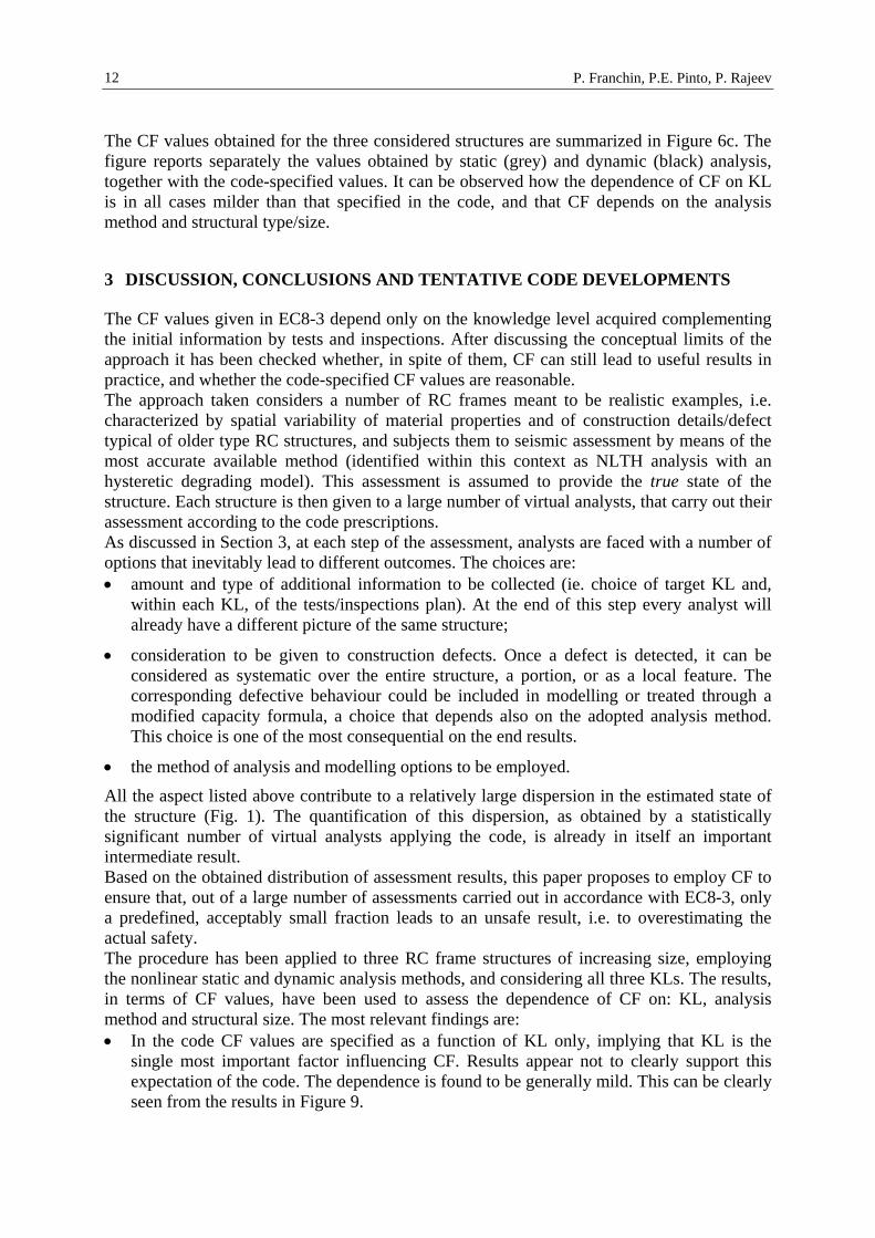
The empirical distributions (conditional on KL) of the 200 Y-values obtained from the curves in Figure 5 is shown in Figure 6a. In the figure the value Y=1 is marked by a dashed vertical line. For the employed seismic intensity of PGA = 0.216g this is the state of the reference structure. A second vertical (solid) line marks the value Y= 0.79. This is the state of the mean structure, i.e. a structure identical in geometry to the reference one, but with spatially homogenous properties (fc, fy, b, sc, sb, ρ) equal to the average values of the samples generated in Step 1. As it can be seen, with increasing KL the distributions get steeper (lower dispersion) and closer to the mean rather then the reference structure. In all cases a large proportion of the analysts overestimates the safety of the structure (i.e. they find Y<1): roughly 40% with KL1, 70% with KL2 and 100% with KL3. Next, the analysis is repeated with CF-values larger than one in order to reduce the above percentages to the same acceptably low value. For the purpose of this application this value has been set to 10%. Sensitivity of the results to this choice can be found in (Rajeev, 2008). Figure 6a shows the corresponding distribution for KL1 only, for clarity (CF=1.34).

0.5 1 1.5 20

0.2

0.4

0.6

0.8

1

Y

F(Y

)

0.5 1 1.5 20

0.2

0.4

0.6

0.8

1

Y

F(Y

)

KL1, CF = 1KL2, CF = 1KL3, CF = 1KL1, CF = 1.34Mean Prop.Limit state

KL1KL2KL3Mean PropertiesLimit state

1

1.05

1.09

1.25

1.19

1.07

1.36

1.25

1.35

1.2

1.111.08

1.21.18

1.34

1.331.31

1.251.25 1.21

1.39

1

1.1

1.2

1.3

1.4

1 2 3

Knowledge Level

Con

fid

ence

Fac

tor

codeabcabc

Fig. 6 a) Structure C, distribution of NVA Y-values obtained by static analysis, b) distribution by static analysis neglecting residual geometric uncertainty, c) CF-values for all structures and analysis types.

The relevance of the residual geometric uncertainty can be appreciated by comparing the curves in Figure 6a with those in Figure 6b, obtained disregarding this contribution (the difference between the structures analyzed by the virtual analysts is only due to material properties and construction defects).


12

The CF values obtained for the three considered structures are summarized in Figure 6c. The figure reports separately the values obtained by static (grey) and dynamic (black) analysis, together with the code-specified values. It can be observed how the dependence of CF on KL is in all cases milder than that specified in the code, and that CF depends on the analysis method and structural type/size.

3 DISCUSSION, CONCLUSIONS AND TENTATIVE CODE DEVELOPMENTS

The CF values given in EC8-3 depend only on the knowledge level acquired complementing the initial information by tests and inspections. After discussing the conceptual limits of the approach it has been checked whether, in spite of them, CF can still lead to useful results in practice, and whether the code-specified CF values are reasonable. The approach taken considers a number of RC frames meant to be realistic examples, i.e. characterized by spatial variability of material properties and of construction details/defect typical of older type RC structures, and subjects them to seismic assessment by means of the most accurate available method (identified within this context as NLTH analysis with an hysteretic degrading model). This assessment is assumed to provide the true state of the structure. Each structure is then given to a large number of virtual analysts, that carry out their assessment according to the code prescriptions. As discussed in Section 3, at each step of the assessment, analysts are faced with a number of options that inevitably lead to different outcomes. The choices are: • amount and type of additional information to be collected (ie. choice of target KL and,

within each KL, of the tests/inspections plan). At the end of this step every analyst will already have a different picture of the same structure;

• consideration to be given to construction defects. Once a defect is detected, it can be considered as systematic over the entire structure, a portion, or as a local feature. The corresponding defective behaviour could be included in modelling or treated through a modified capacity formula, a choice that depends also on the adopted analysis method. This choice is one of the most consequential on the end results.

• the method of analysis and modelling options to be employed.

All the aspect listed above contribute to a relatively large dispersion in the estimated state of the structure (Fig. 1). The quantification of this dispersion, as obtained by a statistically significant number of virtual analysts applying the code, is already in itself an important intermediate result. Based on the obtained distribution of assessment results, this paper proposes to employ CF to ensure that, out of a large number of assessments carried out in accordance with EC8-3, only a predefined, acceptably small fraction leads to an unsafe result, i.e. to overestimating the actual safety. The procedure has been applied to three RC frame structures of increasing size, employing the nonlinear static and dynamic analysis methods, and considering all three KLs. The results, in terms of CF values, have been used to assess the dependence of CF on: KL, analysis method and structural size. The most relevant findings are: • In the code CF values are specified as a function of KL only, implying that KL is the

single most important factor influencing CF. Results appear not to clearly support this expectation of the code. The dependence is found to be generally mild. This can be clearly seen from the results in Figure 9.


13

• The code does not differentiate CF values with respect to the analysis method, implying that epistemic uncertainty has the same effect with all analysis methods. Results appear again not to clearly support this assumption (see Figure 9). When considered separately (i.e. assuming that all analysts will chose the same analysis method) nonlinear static results show a much reduced dispersion than those obtained by nonlinear dynamic analysis. This, according to the proposed procedure, leads in general to smaller values of CF to be employed with static than with dynamic analysis.

• The code does not differentiate the CF values with respect to the structural typology, size or other characteristics. The investigation carried out cannot provide decisive evidence on this aspect due to the number of structures analyzed. However, as it can be seen from Figure 9, the results show a dependence of the CF value on the structure, of the same order as that specified in the code to differentiate between KL1 and KL2.

• The code specifies that the geometry of the structure must be completely known before setting up a model for the analysis. Experience with real-case assessments shows that it is usually not possible to obtain accurate measurements over the entire structure and that even when member centrelines are known, a residual uncertainty on the cross-section dimensions is unavoidable. This source of uncertainty has been modelled in the applications. Results show it to be, for the examined cases, at least of the same order of importance of that associated with material properties and defects.

• The observed importance of the residual geometric uncertainty, indicates the need for some sort of sensitivity study on the corresponding modelling assumptions. It is recalled that the geometric uncertainty has been introduced as a random variation around the mean cross-section height of value ±5cm for KL1, ±2.5cm for KL2 (for KL3 it has been assumed no uncertainty). This is admittedly arbitrary, both in the values themselves and in their graduation with KL. One might well argue that an imprecise evaluation of the cross-section dimensions of ±5cm is still compatible with such a complete state of knowledge as that denoted as KL3. Results under this latter assumption (i.e. no differentiation of geometric uncertainty with KL) have been obtained and reported in (Rajeev, 2008). As expected, the undifferentiated treatment of geometric uncertainty with KL, levels down the differences between KLs. This type of uncertainty (residual on geometry after the data collection process) is not mentioned in the code.

• Finally, there is an interesting aspect not immediately appreciable when following the code prescriptions. The indication of using mean values within the analysis model implies that with increasing KL the average (or median) result of the assessments will not converge to the true state of the structure but, rather, to the state of a mean structure, i.e. a structure identical in geometry to the reference structure but with properties that are spatially homogeneous and equal to the average of those of the reference structure. This fact is quite relevant because while strong spots are lowered towards the mean, the weak spots (which are the critical ones) are raised towards the same mean. Thus, the averaging operation produces in general a structure stronger than the reference one. Hence, on average, the assessment results will converge to a state that is illusorily safer than the actual one.

In conclusion, within the limits of the analyses carried out, it appears that the present state of development of EC8-3 should be improved since: • CF values are not differentiated with respect to analysis method/modelling options;


14

• CF values are not differentiated with respect to structural type (size, regularity, construction material, load-resisting system, etc);

• the so-called complete knowledge (KL3) does not actually correspond to a state of perfect knowledge, hence, it should be penalized with a CF value larger than one;

• there is an important “hidden assumption” in the prescription of using mean values of material properties within the model. This is generally un-conservative, leading on average to underestimating the demand-to-capacity ratio of the structure.

Finally, in more general terms, an aspect that has been highlighted by the study is the large dispersion in assessment results presently allowed by the code. Independently of the CF format, though it is obvious that the code cannot and should not cover prescriptively all the details of the assessment process, many consequential degrees of freedom presently remain in the hands of the analysts, hence stricter guidance would be needed to achieve the goal of more uniform/reliable assessments.

4 ACKNOWLEDGEMENTS

This work has been submitted in a more detailed form to the Journal of Earthquake Engineering. It is presented here as an invited contribution to the Reluis final workshop on proposals for the EC8 “Quali prospettive per l’Eurocodice 8 alla luce delle esperienze italiane”.

5 REFERENCES

European Committee for Standardization (2005) “European Standard EN 1998-3: 2005 Eurocode 8: Design of structures for earthquake resistance. Part 3: Assessment and retrofitting of buildings”, Brussels, Belgium.

Federal Emergency Management Agency. (1997) “NEHRP guidelines for the seismic rehabilitation of buildings,” FEMA 273, Washington, D.C.

Federal Emergency Management Agency. (2000) “Prestandard and commentary for the seismic rehabilitation of buildings,” FEMA Report 356, Washington, D.C.

Iervolino I., Maddaloni G. and Cosenza E., (2008) Eurocode 8 Compliant Real Record Sets for Seismic Analysis of Structures, Journal of Eartquake Engineering, Vol. 12, No. 1, pp.54-90.

Jalayer, F., Franchin, P. and Pinto, P.E. (2007) “A scalar damage measure for seismic reliability analysis of RC frames,” Earthquake Engineering and Structural Dynamics, Vol. 36, No. 13, John Wiley & Sons, NY, USA.

Jalayer F., Iervolino, I. and Manfredi, G. (2008) “Structural modeling uncertainties and their influence on seismic assessment of existing RC structures,” Structural Safety, submitted.

Liu, P. L. and Der Kiureghian, A. (1986) “Multivariate distribution models with prescribed marginals and covariances,” Probabilistic Engineering Mechanics, Vol. 1, No. 2, pp. 105-112

Rajeev P. (2008) “Role of Confidence Factor in Seismic Assessment of Structures” Doctoral Thesis, ROSE School, Pavia, Italy.

Vamvatsikos V. and Cornell C.A. (2002) “Incremental Dynamic Analysis.” Earthquake Engineering and Structural Dynamics, Vol.31, No 3, pp. 491-514.

CONFIDENCE IN THE CONFIDENCE FACTOR

Documents