Concatenation of Lie algebraic maps

4

Concatenat ion of Lie Algebraic Maps

Liam M. Healy and Alex J. Dragt

ABSTRACT Time evolution in a Hamiltonian system may be represented by a transfer map, which in turn may be represented as a product of Lie transformations factored by order. Two such products in succession may be concatenated into a single product. It is possible to do this even when the Lie transformations include inhomogeneous terms. Rules are given for combining and ordering Lie transformations in the general case through sixth order. These rules are presented in an algorithmic fashion suitable for manipulation by computer.

Such techniques have applications to many Hamiltonian systems, including accelerator beam dynamics and optics. The concatenation could repre- sent, for instance, the combined effects of two successive beamline elements in a particle accelerator. In this case, inhomogeneous terms can arise when there are placement, alignment, or powering errors.

4.1 Introduction

In a Hamiltonian system such as a particle accelerator, it is often important to know where a particle will be at a certain time given its position in phase space at some previous time. The relation that gives this information is called the transfer map. This transfer map can be represented by a sequence of Lie transformations factored by order.

It is often desirable to know to a given order the Lie product corresponding to two successive mappings; mathematically we wish to concatenate the two Lie products into one: this is the same as composition of the transfer maps. Treatment of this problem is the primary goal of this paper. One may visualize this, in a particle accelerator, as a means of finding the particular Lie product for the combined effect of two successive beamline elements knowing each separately. This is useful in a variety of calculations. For ex- a:nple, in a single pass system, one can find the combined aberrations of a complete system in terms of the aberrations of its components. Also, when tracking a particle through many turns in a circular accelerator, a great saving in computation time will be realized if many magnetic beamline elements are lumped together as one. Finally, there is an extensive array of analytical tools [8] for analyzing the full one-turn map.

68 Liam M. Healy and Alex J. Dragt

We shall not concern ourselves in this paper with the generation of the original Lie product from the Hamiltonian; that is treated in another paper [12].

4 . 1 . 1 DEFINITIONS AND TERMINOLOGY

It is shown in another paper [12] that the transfer map describing the time evolution of a Hamiltonian system may be represented as a factored product of Lie transformations. Let the transfer map A4 send any point in phase space z to another 5 via the relation

5 = A/I ~l~=z, (1.1)

where ~ = ( q l , P l , . . . , q i , P t ) are the 21 phase space variables, and z is a 21-tuple of values in phase space. Suppose we have a known solution to the time evolution for the orbit through a particular point in phase space. This solution will be called the central orbit. Then, with a suitable choice of coordinates, .£4 may be represented in the neighborhood of the central orbit in the form

A4 = e:A : e: f2:e :fa: . . . (1.2)

Here, fn is a polynomial homogeneous of order n in the phase space variables. The Lze operator :f: associated with f is defined by its action on another function g on phase space,

def :f: g = [f,g]. (1.3)

Here [,] denotes the Poisson bracket. The exponential of a Lie operator is defined by the familiar Taylor series for the exponential,

: f? :f:3 e j ' = z + : / : + 7F., + ' " (1.4)

The exponential of a Lie operator is called a Lie transformation. A Lie transformation e:f~: corresponding to a homogeneous nth-order polynomial is called an nta-order transformation, and the representation of A/l as (1.2) is called the standard faclorization. As shown in [12], the Lie product (1.2) acting on phase space is equivalent to a Taylor series. It should be pointed out that not all maps can be put in the form (1.2); some will require a second second-order transformation, see [12] or [3]. In general we use (1.2) metaphorically.

A Lie algebra is a vector space with a multiplication operation that satisfies linearity,

[ a f + b g , h] = a[ f ,h]+b[g,h] and [f, ag+bh] = a[ f ,a]+b[ f ,h] , (1.5)

antisymmetry, If, g] = -[g, y], (1.6)

4. Concatenation of Lie Algebraic Maps 69

and the Jacobi identity,

[f, [g, hi] + [g, [h, f]] + [h, [f, g]] = 0. (1.7)

There are two primary Lie algebras we use. One is the set of functions on phase space S, of which ~ may be thought a member, with the multiplication operation being a Poisson bracket. The other is the set of Lie operators S* with the multiplication operation being the commutator. There is a homomorphism, or multiplication-preserving map, between these two spaces, called 'Ad'. Because of this homomorphism, these spaces may be thought of interchangeably, and the distinction will not be made henceforth.

The product (1.2) maps S into itself in the following fashion. First, note that the order of the Poisson bracket of two homogenous polynomials is the sum of their respective orders, minus two. That is, the Poisson bracket [fn, gin] is homogenous of order n + m - 2 . From this we may anticipate the resultant order of applying a Lie transformation of a certain order. The ith term in the series (1.4) is : f : / i applied to the previous term. This means

a second-order Lie transformation e:f2: is a linear transformation because each application of :f2: leaves the order of its argument unchanged. By contrast, a third-order transformation e:f3: is non-linear, each application of :f3: increasing the order of its argument by one; a fourth-order tranfor- mation e:f4: is also nonlinear, increasing the order of its argument by two at each application of the operator, and so on. A first-order transformation e:fl:, is a special case. Since :fl: decreases by one the order of its argument, the transformation e:fl: applied to a polynomial results, in general, in terms of all orders down through a constant. In particular, if it acts on the phase space functions ~, it will introduce constant terms. These first- order transformations are the result of inhomogeneities in the Hamiltonian, and have the effect of mapping the central orbit onto some other orbit.

4.1.2 T H E TASK OF CONCATENATION

Suppose now that we have two maps At[ and Af defined by

A4 = e:fl:e:f2:e:f3:...

Af = e:gl:e:g2:e:93:-.-, (1.8)

and we wish to join these into a single map 79,

79 = A4Af. (1.9)

We would like to know how to find the factored form of 79, i.e. the h such that

79 = e:hl:e:h2:e :h3:... (1.10)

In computing this, the number of terms is important. From a practical standpoint, we must truncate each of the products A4 and Af at a certain


order N. It is reasonable to truncate the products 7) at that same value of N. The concatenation problem (1.8-1.10) can then be stated compactly: for a given N, and polynomials f l , . . . , f N and g l , . . . ,gN, we wish to find the polynomials h i , . . . , hN such that

e:ht:e:h2:e:ha: . . . e:hN: ~ e:fl:e:f2:e:fa: . . . e:fN: e:ga :e:g2:e:ga: . . . e:gN:. (1.11)

The symbol ' ~ ' means equivalent through a certain order (in this case N); it will be explained rigorously later. In combining the polynomials, however, higher-order terms will be produced, as we shall see. Furthermore, the presence of first-order terms in the product for one map will combine with any given term of the other product to produce an effect of lower order in the resultant concatenation. These considerations are addressed in the next Section.

4.2 Ideal structure of the Lie algebra

For most realistic maps, the Lie product (1.2) will be infinite. That is, there is no n for which fi - 0 for i _> n. It is of course not practical to deal with an infinite number of terms, so we choose an order at which to truncate the product. This entails making an approximation. This approach is valid in many real physical situations. The Hamiltonian is analytic, so all solutions are analytic in the inital conditions. Therefore, any transfer map is analytic (see [14] chapter 10). We must find a standard by which we can replace a given Poisson bracket by an arbitrary quantity (perhaps zero) if we feel it is "too small," and we must be able to do so consistently. It is crucial not only for derivation of the concatenation formula, but also for calculation of the factored Lie transformation product (1.2) from the Hamiltonian (see [12]). The procedure is divided into two parts: the homogeneous case, where n ~ 2 and m _> 2, and the inhomogeneous, where n = 1 or m = 1. Those not interested in the mathematical underpinnings may without loss of continuity skip to the last paragraph of this Section.

4.2.1 HOMOGENEOUS PRODUCTS

The presumption of the Lie transformation product (1.2) is that the corresponding Taylor series is convergent (see [12]). Since we are truncating this product, we want the remainder term that is omitted to be so small that it can be safely dropped. In order to do this, we take the values of each of the phase space variables to be small so that sufficiently high orders may be ignored. Specifically, let each of the phase space variables carry the small factor 6, so that powers of 6 count the order of these variables. Poly- nomials homogeneous of order n have a factor sn, and will be said to have ~-rank n.


Since 6 is small we may, when taking Poisson brackets, neglect terms with &rank equal to or greater than some specified value N. For example, if we choose N = 6, then the Poisson bracket [f4,gs] may be ignored since it is of order 7. We presently shall give this process some rigor; before doing so however, it is necessary to introduce some definitions. In the mathematical definitions that follow, S stands for an arbitrary Lie algebra and not necessarily the Poisson bracket Lie algebra of phase space functions.

We wish to divide up S by order, consistent with the Lie algebra. To do this, we need the concepts of subalgebra and ideal. A subset S' C S is a subalgebra if 1 [S', S'] C S', where [S', S'] is the image of the Poisson bracket restricted to S'. A subset S' C S is an ideal if IS', S] C S'. That is, for d E S', s E S, then Is', s] E S'. Clearly, an ideal is also a subalgebra. Ideals will play a critical role in the approximation process by way of quotient algebras.

Approximation is made by doing computations in terms of a quotient algebra, which can be defined for any ideal. The ideal plays the role of the remainder, the part that is ignored, and the quotient algebra is the original algebra with "elements approximately the same" identified. Specifically, let I be an ideal in the Lie algebra S. Now define the quotient algebra S/I to be the set of equivalence classes given by the equivalence relation

s l ~ s 2 if s l = s 2 + i for some i 6 I . (2.1)

We denote these classes by s+I, where s E S. Since an ideal is a subalgebra, S/I is a Lie algebra with the rules

(81 + 1) + (82 + 1) = (81 + ~2) + I (2.2)

C(Sl+I ) -cs l+I for c e R (2.3)

[81 + 1,82 q- I] = [81,82] "4- I . (2.4)

These rules are easily seen to be consistent. If il, i2 E I are arbitrary, the left side of the first rule (2.2) is

(8, + il) + (82 + i2) = (81 + s2) + (i, + i2) e (81 + s2) + 1, (2.5)

since I is a vector subspace of S . A similar argument holds for the second rule. The left side of the third rule (2.4) is

[81 + il , S2 + i2] = [81, S2] + [Sl, i21 + [il, S2] + [il, i2]. (2.6)

1The notation [X, Y] where X and Y are sets means the set

{[~,v] I • E x , v E Y}.


From the definition of an ideal, we see that the consistency of the third rule is upheld.

Now we address ourselves to the question of the origin of the ideals for the approximation. They come from a percolation, a telescoped set of subspaces whose union fill the whole space and whose Lie bracket fulfills a certain property: for each non-negative integer i, there is a subspace S(i) such that

S (i) D S (j) for i < j (2.7)

s(°) = s (2.8)

[S (i), S (j)] C S (i+j) . (2.9)

I f S is graded, that is, it is the direct sum of subspaces Si (i = 0, 1 , . . . ,oo) and [S,, Sj] C Si+j, then it is percolated by the rule

S(, ) dJ 0 Sj. (2.10) j_>i

In our application, these subspaces will be polynomials of a certain b-rank or higher.

It is clear from the above definition that each of the members S(0 of a percolation is an ideal. Let s(0 E S (i), s E S = S (°). Then [s, s( i)] E S(0, and also with the arguments in the reverse order, [s(1),s] E S(0. Since s and s (i) were arbitrary within their respective sets, S(i) is an ideal in S .

Let us now apply this to our particular problem. Up to now in this Section, we have let S stand for an arbitrary Lie algebra. We now restrict the definition of S so that it is the space of all functions on phase space that have power series expansions and whose power-series expansion has no first-order or constant term. Grade it with subspaces of polynomials homogeneous in a particular order of the phase space variables: let Si be the set of all homogeneous polynomials of order i + 2, for i > 0. One may easily verify that this is a grading on S under the Poisson bracket. A particular polynomial that belongs to the subspace S, has b-rank i + 2.

Given this grading {S, } by polynomial order, we have the corresponding percolation given by (2.10). This gives us a sequencs of ideals S (i), and a sequence of quotient algebras S/S(') . The ideal S(') consists of all power series with coefficients zero for all terms of order less than i+ 2. The quotient algebra Q(i) de f S/s(i+I) is a rigorous way of describing the algebra S with the approximation of "neglecting terms of order i + 3 and greater."

The computer code MArtYLIE 3.0 [2] [6] [7], designed to perform beam dynamics calculations for accelerator physics, has no first-order polynomials and performs computat ions through fourth order. Speaking in terms of the formal algebra introduced above, it is computing in the Lie algebra Q(~). In this algebra, one must say, for example, [f3,g3] = h4 for some specific h4, but it makes the approximation [f3, 94] ~ 0. In the algebra Q(2) the values of some Poisson brackets will be in S 3. Since we are working in


the quotient algebra, we may choose any member of S 3. When performing the computation by hand, we will usually choose zero. When working nu- merically in a computer code (the tracking part of MARYLIE), the choice of some other members may be computationally advantageous.

The homomorphism Ad carries all these definitions to the adjoint algebra S* . The subalgebras S *(i) are the spaces of all Lie operators that are of order i + 2, i.e., are images of Si under Ad, and S *(i) are the direct sum ~3j>iS~ or the image of S (i) under Ad. The S*(0 are ideals, so the

Q.(i) = S . / S , ( i + I ) are quotient algebras. Thus the adjoint algebra has the same ideal and quotient structure as the underlying algebra, as we expect, and commutators of Lie operators are set to zero (or to an arbitrary value) when the Poisson bracket of the corresponding polynomials would be of too high an order.

These quotient Lie algebras give rise to quotient groups in the group of all symplectic maps on phase space. While possibly containing terms of all orders, these maps are accurate only through order i + 1 for Q(i). Within the group, it will be possible to either truncate and then multiply, or multiply and then truncate, with equal validity. Specifically, let G be the group of symplectic maps on phase space and G (i) (i = 0, 1, . . . ) be the subgroup of these maps that has a power series expansion consisting of terms only order i + 1 and higher, plus the identity. Then G(') is a normal or invariant subgroup of G, that is, ghg -1 E G (i), Vg E G, h E G (i). The quotient group H (i) = G / G (i+l) is defined as the equivalence classes given by gl ~ g2 if glg~ 1 = h where h E G (i). That is, two elements are equivalent if the power series expansions of their associated symplectic maps differ only by terms of order i + 1 and higher. That this is in fact a group may be easily verified. These groups H (i) are associated with the algebras Q*(').

4.2.2 INHOMOGENEOUS PRODUCTS

If a first-order transformation is present in the product (1.2), the truncation by &rank given above will not be correct because the &rank will be lowered by the first-order term. Suppose we keep terms only through &rank 4, and discard anything higher. Then forming, for instance, [fl, [g3, h4]] would yield the wrong answer: we may take [g3, hal as zero because the 6-rank is 5, and so our overall answer would be zero. But this is not correct; even though the inner Poisson bracket is 6-rank 5, the Poisson bracket with f l subsequently lowers the &rank to an acceptable 4. Clearly, the subspaces described in the last Section are no longer subalgebras when a first-order term is present and we must reformulate their description for correct computations in this case.

The correct t reatment of first-order terms becomes evident when we consider their physical origin. As is shown in [12], the first-order transformation is proportional to the first-order term in the Hamiltonian, which in turn is proportional to an error, such as an alignment or powering error in an ac-


celerator beamline element. It is hoped that these are small; consequently, the first-order transformation will also be small. To be specific, say that a factor of the small parameter e multiplies each first-order polynomial. We may now consider how this changes the analysis of the algebra and the corresponding group given in the previous Section.

The space S must be expanded, and the set {S/} given a new member. Let S now stand for the set of all functions on phase space that have power- series expansions; we no longer require that the first-order term be zero. We shMl still ignore constant terms since they play no role in the Lie algebra. Let S-a be the space of first-order polynomials. The spaces {Ss],=-l,0,1,. are still a grading. However, we cannot construct a corresponding percolation according to (2.10) because we now have a negative i. Thus the S (/) are no longer ideals and we cannot form the quotient algebra. There is a corresponding destruction of the normal subgroups and quotient groups of symplectic maps.

Instead of using this grading, let us search for another way to create a percolation, and thus obtain a sequence of ideals and a sequence of quotient Mgebras that will correctly reflect the physics of the perturbation calculation. First, let the e-rank of a polynomial mean the lowest order in e for that polynomial. Define a second index j , j -- 0, 1, . . . , on the S/ that is equal to the e-rank. Thus Sir is a subset of S that is homogeneous of order i + 2 in the phase space coordinates, and homogeneous of order j in e. A polynomial has 6-rank i and e-rank j if it belongs to Sir. The only combination of i and j within these ranges that is prohibited is i = - 1 , j = 0, the smallness requirement on first-order terms discussed above. The spaces Sis are a finer grading of the spaces Ss graded by 6-rank; it is easy to see that

[Sir, Skz] c_ Si+k, +z. (2.11)

We now seek a percolation constructed from the S,j. A percolation that satisfies the requirements may be formed by creating

a special function of the two indices i and j . Consider the set of allowed index pairs

][2. def {- -1 ,0 ,1 , . . .} X {0, 1 , . . . } - - {(--1,0)]. (2.12)

Let a truncalzon criterion u be any function into the non-negative integers u : ][2, ~ ][+ with the property

+ <_ + k , j + t). (2.13)

Now define the sequence of subspaces S (i), i E Z + as the direct sum of all Sjk whose value of u is at least i:

s(') (9 (2.14) ~(j,k)>i


This sequence is a percolation, which may be shown in the following man- ner. Clearly, the first and second properties of a percolation are satisfied. To show the third (2.9), let Si,j, be an arbitrary element of S (~(i,j)) and Sk,z, be an arbitrary element of S (~(k,0). Then

Si,j, E S (v(i'j)) :=~ u(i ' , j ' ) >_ u(i , j ) (2.15)

Sk,z, 6 S (v(k'0) =~ u(k' , l ' ) > u(k,l). (2.16)

The Poisson bracket of these two polynomial spaces is

[Si,~,,S~,t,] c_ &,+k,,~,+z, c_s (~(v+k''~'+e)) S (v(i''jt)+t/(k''l')) C S (v(i'j)+v(k'l)), (2.17)

by the truncation criterion (2.13) and the first property of a percolation (2.7). Since Si,j, and Sk,t, were arbitrary in their respective subspaces, we may conclude the third property of a percolation holds,

[S('~) , S (m)] C_ S(n+m) , (2.18)

for values n, m in the image of u. By implication, therefore, the S(i) as defined in (2.14) are ideals. This sequence of ideals may be used to define a sequence of quotient algebras.

Note that we have determined a satisfactory set of ideals with u unde- termined except for the condition (2.13). We now must consider specific truncation criteria. Two possibilities are u(i, j ) = rain(i, j ) and u = a i+ f l j where a,/3 E Z + • The reader may verify that these two indeed satisfy (2.13). The former case corresponds to keeping all terms except those whose 6- rank and whose e-rank each exceed a certain value. The latter excludes those whose weighted sum exceeds a certain value. This form of t, satisfies a stricter condition than (2.13), in fact, u(i , j ) + u(k,l) = u(i + k , j + l), and so we have a grading S~(,,j), which may form a percolation by (2.10). This percolation is the same as the one defined by (2.14).

Normal subgroups G("(i,J)) of the group of inhomogeneous symplectic maps G may be defined by analogy to that of the homogeneous group (see

Section 4.2.1). The quotient group H (u(iJ)) dej G/G(u(i,j) ) is the group of transformations that will actually be used in computations.

With all the formalism aside, we must choose a particular truncation criterion with which to proceed with the actual computations. The one that makes the most intuitive sense is u(i , j ) = i + j . This will be called the total rank. In terms of 6-rank and e-rank, this criterion says that we restrict terms to 0(6) + O(¢) < N for some value of N. Physically, this is a realistic criterion, because it means that the deviation in central orbit caused by the error is of the same order as the perturbation around the central orbit. Thus, we can expect the same accuracy in the result. For example, the misalignment of a magnetic element in an accelerator should not typically


be of greater magnitude than the spread in position of particles within the beam. It is also possible to imagine the case where a different truncation criterion needs to be used; for instance, a weighted sum of the exponents as mentioned above may be appropriate. The calculations in the remainder of this paper, however, are done with the total rank criterion.

4.3 Lie algebraic tools

With the algebraic formalism established, we now turn to the problem of solving the concatentation problem (1.11). There are two important tools used in this calculation that are presented in this Section. At the moment, it is useful to introduce some notation. It will become necessary to label a polynomial by its total rank as well as its ~i-rank. In this case, a superscript with the total rank in parenthesis will be placed on the polynomial, e.g., k (4). Furthermore, let the function r give tile total rank of a polynomial or

operator, so that, e.g., r(k (4)) = 4. In Section 4.4.2 this notation will be generalized slightly; the superscript will identify a family of terms of which at least one is of that total rank, none are lower, and some may be higher.

4.3.1 T H E EXCHANGE RULE

The first tool used in the computation is the exchange rule. This allows us to rewrite two Lie transformations in succession such that one transformation occurs in the opposite position,

e:f:e:g: = e:J:e :f: (3.1)

o r

e:f:e :g: -- e:g:e :k:, (3.2)

where the polynomials are not necessarily homogeneous. The function j in (3.1) is given by

j -- e: f:g (3.3)

and the function k in (3.2) is given by

k = e : - g : f . (3.4)

For proofs, see [4] (Theorem 3), [2], or [3] (equation 5.52). It is also possible to bring a Lie transformation inside a function; that is,

e : / :g(( ) = g(e:/:~), (3.5)

for arbitrary functions f , g. This is proved in [3] and in [2]. In combination with the exchange rule, we have a powerful result because it means that


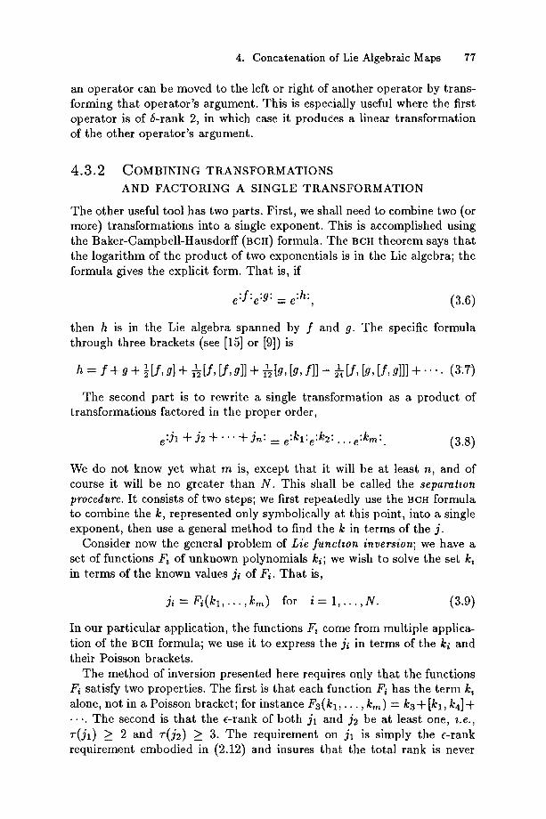
an operator can be moved to the left or right of another operator by transforming that operator's argument. This is especially useful where the first operator is of 6-rank 2, in which case it produces a linear transformation of the other operator's argument.

4.3.2 COMBINING TRANSFORMATIONS AND FACTORING A SINGLE TRANSFORMATION

The other useful tool has two parts. First, we shall need to combine two (or more) transformations into a single exponent. This is accomplished using the Baker-Campbel]-Hausdorff (BCH) formula.. The BCH theorem says that the logarithm of the product of two exponentials is in the Lie algebra; the formula gives the explicit form. That is, if

e:f:e:g: = e :h:, (3.6)

then h is in the Lie algebra spanned by f and g. The specific formula through three brackets (see [15] or [9]) is

1 1 f 1 . h = f + g + ~[f, g] + i~[ , [f, g]] + ~[g, [g, f]] - ~ [ f , [g, [f, g]]] + " " (3.7)

The second part is to rewrite a single transformation as a product of transformations factored in the proper order,

e:Jl + j2 + " " + jn: = e:kl:e:k2: . . .e:km:. (3.8)

We do not know yet what m is, except that it will be at least n, and of course it will be no greater than N. This shall be called the separatzon procedure. It consists of two steps; we first repeatedly use the BCH formula to combine the k, represented only symbolically at this point, into a single exponent, then use a general method to find the k in terms of the j .

Consider now the general problem of Lie func twn inversion; we have a set of functions F, of unknown polynomials ki; we wish to solve the set k, in terms of the known values ji of F i. That is,

Ji = F i ( k l , . . . , k m ) for i = l , . . . , N . (3.9)

In our particular application, the functions F, come from multiple application of the BCH formula; we use it to express the ji in terms of the ki and their Poisson brackets.

The method of inversion presented here requires only that the functions F{ satisfy two properties. The first is that each function Fi has the term k, alone, not in a Poisson bracket; for instance F3(k l , . . . , kin) -- k3"]-[kl, k4]n t- • ... The second is that the e-rank of both j l and J2 be at least one, z.e., 7-(jl) > 2 and 7"(j2) >_ 3. The requirement on j l is simply the c-rank requirement embodied in (2.12) and insures that the total rank is never


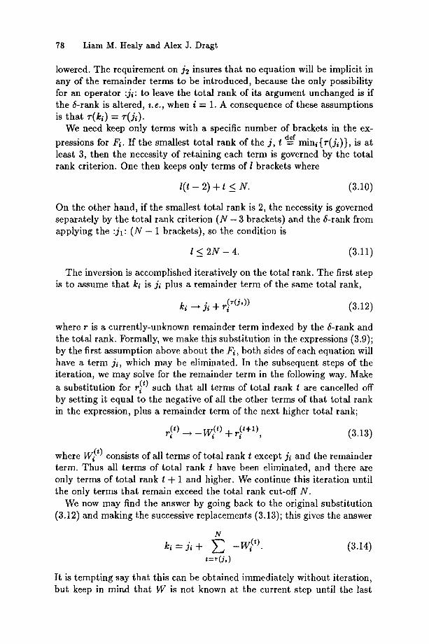
lowered. The requirement on j2 insures that no equation will be implicit in any of the remainder terms to be introduced, because the only possibility for an operator :ji: to leave the total rank of its argument unchanged is if the 5-rank is altered, i.e., when i = 1. A consequence of these assumptions is that r (k i ) = r ( j i ) .

We need keep only terms with a specific number of brackets in the ex- def

pressions for F~. If the smallest total rank of the j , t = mini{v(ji)}, is at least 3, then the necessity of retaining each term is governed by the total rank criterion. One then keeps only terms of I brackets where

l( t - 2) + t < N. (3.10)

On the other hand, if the smallest total rank is 2, the necessity is governed separately by the total rank criterion (N - 3 brackets) and the $-rank from applying the :jl: (N - 1 brackets), so the condition is

l _< 2N - 4. (3.11)

The inversion is accomplished iteratively on the total rank. The first step is to assume that ki is j i plus a remainder term of the same total rank,

_(~U,)) (3.12) kl "-'+ j i + "i

where r is a currently-unknown remainder term indexed by the 5-rank and the total rank. Formally, we make this substitution in the expressions (3.9); by the first assumption above about the Fi, both sides of each equation will have a term j i , which may be eliminated. In the subsequent steps of the iteration, we may solve for the remainder term in the following way. Make a substitution for r} t) such that all terms of total rank t are cancelled off by setting it equal to the negative of all the other terms of that total rank in the expression, plus a remainder term of the next higher total rank;

_(,+i) __, _w,¢ , ) + , . , , (3.13)

where W (t) consists of all terms of total rank t except j i and the remainder term. Thus all terms of total rank t have been eliminated, and there are only terms of total rank t + 1 and higher. We continue this iteration until the only terms that remain exceed the total rank cut-off N.

We now may find the answer by going back to the original substitution (3.12) and making the successive replacements (3.13); this gives the answer

N

k, = j, + E -W(0" (3.14) t=r(j , )

It is tempting say that this can be obtained immediately without iteration, but keep in mirLd that W is not known at the current step until the last

4. Concatenation of Lie Algebr~dc Maps 79

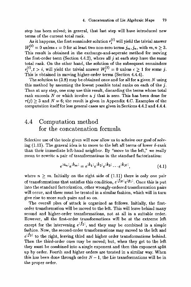
step has been solved; in general, that last step will have introduced new terms of the current total rank.

As it happens, the first remainder solution r~ 0 will yield the trivial answer

W (0 = 0 unless e = 0 for at least two non-zero terms jm , jn , with m, n > 3. This result is obtained in the exchange-and-seperate method for moving the first-order term (Section 4.4.2), where all j at each step have the same total rank. On the other hand, the solution of the subsequent remainders r~ t), t > i, will yield the trivial answer W (t) = 0 unless e >_ 1 for some j . This is obtained in moving higher-order terms (Section 4.4.4).

The solution to (3.8) may be obtained once and for all for a given N using this method by assuming the lowest possible total ranks on each of the j . Then at any step, one may use this result, discarding the terms whose total rank exceeds N or which involve a j that is zero. This has been done for r ( j ) >_ 3 and N = 6; the result is given in Appendix 4.C. Examples of the computation itself for less general cases are given in Sections 4.4.2 and 4.4.4.

4.4 Computation method for the concatenation formula

Selective use of the tools given will now allow us to acheive our goal of solving (1.11). The general idea is to move to the left all terms of lower 5-rank than their immediate left-hand neighbor. By "move to the left," we really mean to rewrite a pair of transformations in the standard factorization:

e:an:e:bm : = e:kl:e:k2:e:kz: . . . e:kN :, (4.1)

where n _> m. Initially on the right side of (1.11) there is only one pair

of transformations that satisfies this condition, e:fN:e:gl:. Once this is put into the standard factorization, other wrongly-ordered transformation pairs will occur, and these must be treated in a similar fashion, which will in turn give rise to more such pairs and so on.

The overall plan of attack is organized as follows. Initially, the first- order transformation will be moved to the left. This will leave behind many second and higher-order transformations, not at all in a suitable order. However, all the first-order transformations will be at the extreme left

except for the intervening e : f 2:, and they may be combined in a simple fashion. Now, the second-order transformations may moved to the left and

e:f2: to the right, leaving third and higher order transformations behind. Then the third-order ones may be moved; but, when they get to the left they must be combined into a single exponent and then this exponent split up by order. Fourth and higher orders are treated in a similar way. When this has been done through order N - 1, the Lie transformations will be in the proper order.

80 Liam M. ttealy and Alex J. Dragt

The basic methods for treating pairs of transformations (4.1) are presented in the next Section, and the actual procedure for each order m in the succeeding Sections. As an alternative to the pairwise treatment of terms described above and elaborated below, one may try to combine all the terms

of the concatenation problem (1.11) except e:f2: and e:g~: at once using an expanded version of the combine-and-separate method described in the next Section. This has a certain conceptual simplicity, but it is not practical as it would generate an inordinate number of terms for even small N.

4.4.1 P U T T I N G A PAIR OF TRANSFORMATIONS

INTO STANDARD FACTORIZATION

For the task of putting two successive transformations into standard factorization (4.1), there are three possibilities. If m -- 2 and r(b2) -- 2, there is no choice but to use the exchange method. If this is not the case, there are two choices.

The exchange-and-separate method uses the exchange rule to write

e:an:e :bin: -: e:bm:e :e:-bm:an: = e:bm:e :an+:-bm:an + . . . . , (4.2)

and then application of the separation procedure on the second transformation. Because the transformation e :bin: remains separate on the left, this method is not useful for the case m = n. It is advantageous for m = 1 because all terms in the second transformation have total rank at least 3, reducing the number of Poisson brackets required.

The combine-and-separate method uses the SCH formula to combine the terms into a single exponent,

1 e:an:e:bm: = e:an +bm "4- ~[an,bm] A- " " : , (4.3)

and then application of the separation procedure on this transformation. This method is preferable when m > 1 and necessary when m = n. Note that this incarnation of the BCH formula is distinct from that of the separation procedure that produces the functions Fi in (3.9); this is the combination of only two terms and changes at each step.

4.4.2 MOVING THE FIRST-ORDER TERM

We concentrate initially on the terms f3 through gl of (1.11) and temporarily ignore the other Lie transformations. That is, we wish to put

e :fl:e:f2:e : f3: . . . e:fN:e :gl: (4.4)

into standard factorization. This is done successively on each transformation; we start by putting the right-hand pair with f g and gl into standard


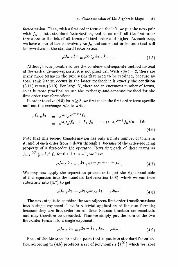
factorization. Then, with a first-order term on the left, we put the next pair with f N - 1 into standard factorization, and so on until all the first-order terms are to the left of all terms of third order and higher. At each step, we have a pair of terms involving an f , and some first-order term that will be rewritten in the standard factorization,

e:f'~:e :bl: = e:kl:e:k2:e :k3: . . . . (4.5)

Although it is possible to use the combine-and-separate method instead of the exchange-and-separate, it is not practical. With r(bl) = 2, there are many more terms in the BCH series that need to be retained, because no total rank 2 term occurs in the latter method; it is exactly the condition (3.11) versus (3.10). For large N, there are an enormous number of terms, so it is more practical to use the exchange-and-separate method for the first-order transformations.

In order to solve (4.5) for n > 3, we first make the first-order term specific and use the exchange rule to write

e:fn:e:bl: = e:bl:e:e:-bl: fn:

= e:bl :e : f , + [ - b , , I , ] + - . . + : - b , : "-1 I n / ( - - 1)!:.

(4.6)

Note that this second transformation has only a finite number of terms in it, and of each order from n down through 1, because of the order-reducing property of a first-order Lie operator. Rewriting each of these terms as

d e f j,~_~ = ~ : - b l : ~ fn for 0 < i < n - 1, we have

• f,~" "bl" e:bl:e:jl + j2 + " " + jn: (4.7) e" "e" " - -

W e may now apply the separation procedure to put the right-hand side of this equation into the standard factorization (3.8), which we can then substitute into (4.7) to get

e:fn:e :bl: = e:b l :e:k l :e :k2: . . . e :km:. (4.8)

The next step is to combine the two adjacent first-order transformations into a single exponent. This is a trivial application of the BCH formula; because they are first-order terms, their Poisson brackets are constants and may therefore be discarded. Thus we simply put the sum of the two first-order terms into a single exponent:

e:fn:e:bl: = e :bl + kl:e:k2: . . , e :k'n:. (4.9)

Each of the Lie transformation pairs that is put into standard fa.ctoriza-

tion according to (4.5) produces a set of polynomials {k~ t)} which we label


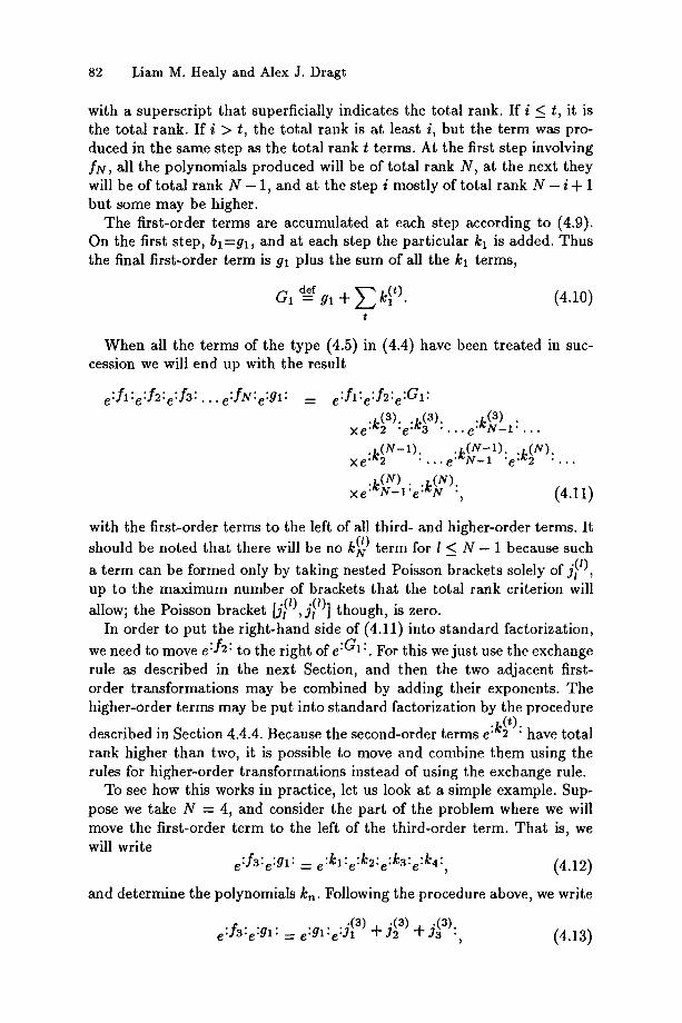
with a superscript that superficially indicates the total rank. If i < t, it is the total rank. If i > t, the total rank is at least i, but the term was produced in the same step as the total rank ¢ terms. At the first step involving f g , all the polynomials produced will be of total rank N, at the next they will be of total rank N - 1, and at the step i mostly of total rank N - i + 1 but some may be higher.

The first-order terms are accumulated at each step according to (4.9). On the first step, bl=gl, and at each step the particular kl is added. Thus the final first-order term is gl plus the sum of all the kl terms,

a l .1 + (4.10) t

When all the terms of the type (4.5) in (4.4) have been treated in succession we will end up with the result

e:f l :e: f2:e: f3: . . .e: fN:e:gl: = e:/l:e:f~:e:G1: .b(3) . .b(3) . .k(3) .

xe'~2 "e'~3 " . . .e" g - 1 . . . . (. . . . . k ( N - 1 ) . . ] ¢ ( N ) .

xe:k- N-l): e" N-1 "e" 2 - . . .

x e:k(NN-)l :e :k(N): , (4.11)

with the first-order terms to the left of all third- and higher-order terms. It should be noted that there will be no k~ ) term for l _< N - 1 because such

a term can be formed only by taking nested Poisson brackets solely of j}0, up to the maximum number of brackets that the total rank criterion will allow; the Poisson bracket [j}0,j}0] though, is zero.

In order to put the right-hand side of (4.11) into standard factorization,

we need to move e:f2: to the right ofe :GI:. For this we just use the exchange rule as described in the next Section, and then the two adjacent first- order transformations may be combined by adding their exponents. The higher-order terms may be put into standard factorization by the procedure

described in Section 4.4.4. Because the second-order terms e:k~ ~): have total rank higher than two, it is possible to move and combine them using the rules for higher-order transformations instead of using the exchange rule.

To see how this works in practice, let us look at a simple example. Sup- pose we take N - 4, and consider the part of the problem where we will move the first-order term to the left of the third-order term. That is, we will write

e:fa:e :gl: = e:kl:e:k2:e:ka:e :k4:, (4.12)

and determine the polynomials kn. Following the procedure above, we write

e:f3:e:gl: _ e:gl:e:j~3) + j~3) + j(a):, (4.13)


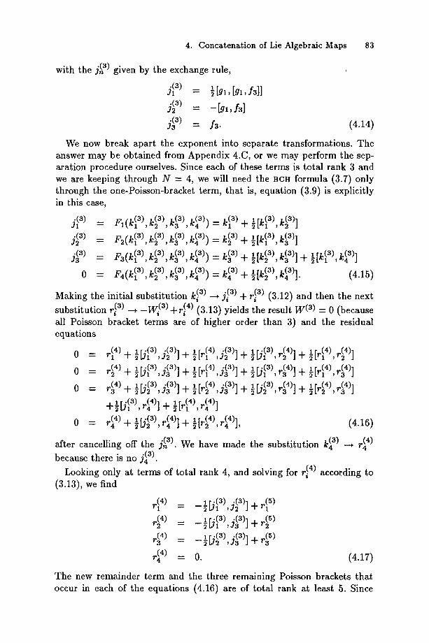
with the j(3) given by the exchange rule,

1 j~3) = ~[gl, [gl, f3]]

j~a) : - [gl , f3]

(4.14)

We now break apart the exponent into separate transformations. The answer may be obtained from Appendix 4.C, or we may perform the separation procedure ourselves. Since each of these terms is total rank 3 and we are keeping through N - 4, we will need the BCIt formula (3.7) only through the one-Poisson-bracket term, that is, equation (3.9) is explicitly in this case,

j~3) F %(3)k(3)k(3) k(3)) k~3) - - 21, 1 , 2 , 3 , - - "~-

,,.(3)¢3) --" 31,t~i ' 2 ' 3 ~ --" -~

b 0 "-- ~'41,a;I ' ~ 2 ' : "31-

tk?),kl 3)1 rt.(3) t.(3)1 t n ' l , '~3 J

1 rk(3) k(3)l 1 rk(3) k(43)] 2L 2 ' 3 ,J'*'lt-2t 1 ,

1 [L,(3) b(3)l (~t .t,.~)(A.1K'~ L"2 ''4 J"

Making the initial substitution k~ 3) --~ j~3) + r~3) (3.12) and then the next substitution r~ 3) ~ - W (3) +r~ 4) (3.13) yields the result W (3) = 0 (because all Poisson bracket terms are of higher order than 3) and the residual equations

, r~(3) ~(3)1 , [r~4), 0 ---- r ~ 4) -4- ~l, J1 , J 2 J "~ 5

1 rZ(3) Z(3)1 1 [ r~4 ) , 0 = r ( 4 ) "4- ~L]I , J 3 J -]-

l r ~ ( 3 ) ,;(3)1 1 [ r~4 ) , 0 : r ( 4 ) + ~1,12 , J 3 J +

. 4 _ 1 r . ( 3 ) (4) , 1 [ r ( 4 ) r i 4 ) ] 5 U I , r 4 J - l - ~ L I ,

r~(3) ~(4)i ~ [r~4), 0 = r (4)%~. ,-4 J%

after cancelling off the j(3). We have because there is no j(3).

Looking only at terms of total rank (3 .13) , we find

,r.(3) (4), ~ rr(4) r~4)] j ( 3 ) ] + ~ p l ,r2 J+~L 1 , r~(3) . (4 h 1 r~(4) ~(4)1 J3 (3)] + ~ m , - 3 J + ~ t - i , - 3 ,

r,~(3) .(4)1 ~ r..(4) ..(4)1 J3 (3)] + ~ ~2 , ' 3 J + ~t-2 , - 3 J

r(4)], (4.16)

made the substitution k (3) --~ r l 4)

4, and solving for r~ 4) according to

ri4) _ 1.(3) + ; t ) - - - - ~ t./2 ,

r(44) : 0. (4.17)

The new remainder term and the three remaining Poisson brackets that occur in each of the equations (4.16) are of total rank at least 5. Since


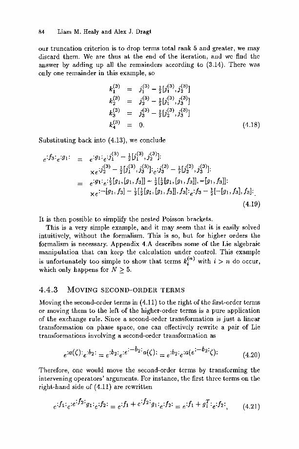
our truncation criterion is to drop terms total rank 5 and greater, we may discard them. We are thus at the end of the iteration, and we find the answer by adding up all the remainders according to (3.14). There was only one remainder in this example, so

k~3) = jr3) lr;(3) ;(3), -- ~LJ1 , J2 J k ? ) : l r(3)

- - [ [ J 1 , 3 3 J

k(3) -- J3 ( 3 ) - !r;(3)~tJ2 ,J (3)13 J

k (3) = 0.

Substituting back into (4.13), we conclude

e:f3:e:gl:

(4.18)

: e:gl:e:J? ) - xe : J~ 3) -- ~[.]11 r .(3),33"(3)l"J'e :']3"(3) _ ½ [j~3), j3(3)]:

_ - e'g"e'~" " " l [g~ , [g , , f3 ] ] - ~[½[g~,[gi,f3]],-[m,/3]]:

Xe:--[gl, f3] -- ½[½[gl, [gl, f3]], f3]:e:f3 -- ½[--[gl, f3], f3]:.

(4.10)

It is then possible to simplify the nested Poisson brackets. This is a very simple example, and it may seem that it is easily solved

intuitively, without the formalism. This is so, but for higher orders the formalism is necessary. Appendix 4.A describes some of the Lie algebraic manipulation that can keep the calculation under control. This example is unfortunately too simple to show that terms k~ n) with i > n do occur, which only happens for N > 5.

4 . 4 . 3 MOVING SECOND-ORDER TERMS

Moving the second-order terms in (4.11) to the right of the first-order terms or moving them to the left of the higher-order terms is a pure application of the exchange rule. Since a second-order transformation is just a linear transformation on phase space, one can effectively rewrite a pair of Lie transformations involving a second-order transformation as

e:a(~):e :b2: - e:b2:e:e:-b2:a( ~): -- e:b2:e :a(e:-b2:~): (4.20)

Therefore, one would move the second-order terms by transforming the intervening operators' arguments. For instance, the first three terms on the right-hand side of (4.11) are rewritten

e:fl:e:e:f2:gl:e:f2: = e:fl + e:f2:gl:e:f2: = e:fl + gT:e:f2: ' (4.21)


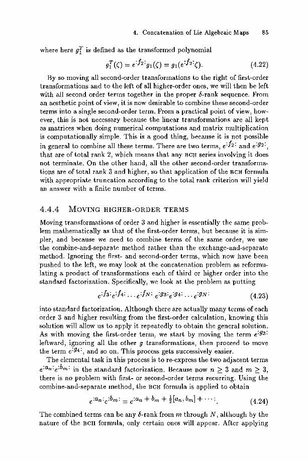
where here gT is defined as the transformed polynomial

gT(~) = e: f2:gl(~) = gl(e: f2:~) . (4.22)

By so moving all second-order transformations to the right of first-order transformations and to the left of all higher-order ones, we will then be left with all second order terms together in the proper &rank sequence. From an aesthetic point of view, it is now desirable to combine these second-order terms into a single second-order term. From a practical point of view, however, this is not necessary because the linear transformations are all kept as matrices when doing numerical computations and matrix multiplication is computationally simple. This is a good thing, because it is not possible

in general to combine all these terms. There are two terms, e:f2: and e :g2:, that are of total rank 2, which means that any BCH series involving it does not terminate. On the other hand, all the other second-order transformations are of total rank 3 and higher, so that application of the BCH formula with appropriate truncation according to the total rank criterion will yield an answer with a finite number of terms.

4.4.4 MOVING HIGHER-ORDER TERMS

Moving transformations of order 3 and higher is essentially the same problem mathematically as that of the first-order terms, but because it is simpler, and because we need to combine terms of the same order, we use the combine-and-separate method rather than the exchange-and-separate method. Ignoring the first- and second-order terms, which now have been pushed to the left, we may look at the concatenation problem as reformu- lating a product of transformations each of third or higher order into the standard factorization. Specifically, we look at the problem as putting

e:f3:e : f 4 : . . . e : fN: e:g3:e :g4: . . . e :gN: (4.23)

into standard factorization. Although there are actually many terms of each order 3 and higher resulting from the first-order calculation, knowing this solution will allow us to apply it repeatedly to obtain the general solution. As with moving the first-order term, we start by moving the term e :g3: leftward, ignoring all the other g transformations, then proceed to move the term e:g4:, and so on. This process gets successively easier.

The elemental task in this process is to re-express the two adjacent terms

e:a'*:e :bin: in the standard factorization. Because now n >_ 3 and m > 3, there is no problem with first- or second-order terms recurring. Using the combine-and-separate method, the BCH formula is applied to obtain

• " 1 [ a n , b i n ] + ' " : e.an : e :bm : =. e.an "-b bm "b "~ (4.24)

The combined terms can be any &rank from m through N, although by the nature of the Ben formula, only certain ones will appear. After applying


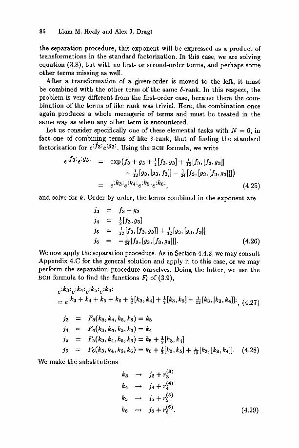
the separation procedure, this exponent will be expressed as a product of transformations in the standard factorization. In this case, we are solving equation (3.8), but with no first- or second-order terms, and perhaps some other terms missing as well.

After a transformation of a given-order is moved to the left, it must be combined with the other term of the same 8-rank. In this respect, the problem is very different from the first-order case, because there the combination of the terms of like rank was trivial. Here, the combination once again produces a whole menagerie of terms and must be treated in the same way as when any other term is encountered.

Let us consider specifically one of these elemental tasks with N = 6, in fact one of combining terms of like 8-rank, that of finding the standard factorization for e:f3:e :g3:. Using the BCH formula, we write

e:f3:e :g3: = exp(f3 + g3 q- ½[fa,g3] q- 1~[f3, [fz,g3]]

q- ~[g3, [g3, f3]] -- ~[f3, [g3, If3, g3]]])

: e:k3:e:k4:e:ks:e :k6:, (4.25)

and solve for k. Order by order, the terms combined in the exponent are

j3 = f a T g 3 J4 = ½ [f3, g3]

j5 = ~ [fa, [f3, g3]] + ~[g3, [ga, fa]] j6 = -- ~[ fa , [g3, [f3, g3]]]. (4.26)

We now apply the separation procedure. As in Section 4.4.2, we may consult Appendix 4.C for the general solution and apply it to this case, or we may perform the separation procedure ourselves. Doing the latter, we use the BCH formula to find the functions Fi of (3.9),

e:ka:e:k4:e:ks:e:k6: 1 1 = e:k3 + k4 + k5 + k6 + 5[k3, k4] + ~[k3, ks] + ~[k3, [k3, k4]]:, (4.27)

3 ~- =

j5 =

j6 =

We make the substitutions

F 3(k3 , k4, k5, k6) - - k3

F4(k3, k4, ks, k6) = k4 Fs(k3, k4, ks, k6) k5 + = ½[k3,k,]

1 r6(k3, k,, ks, k6) = + [k3, ks] + [k3, k,]].

k3- j3+ (2 )

k4 --, j4+r~ 4)

k5 -~ j 5 + r ~ 5)

k6 ~ j 6 + r ~ 6).

(4.28)

(4.29)


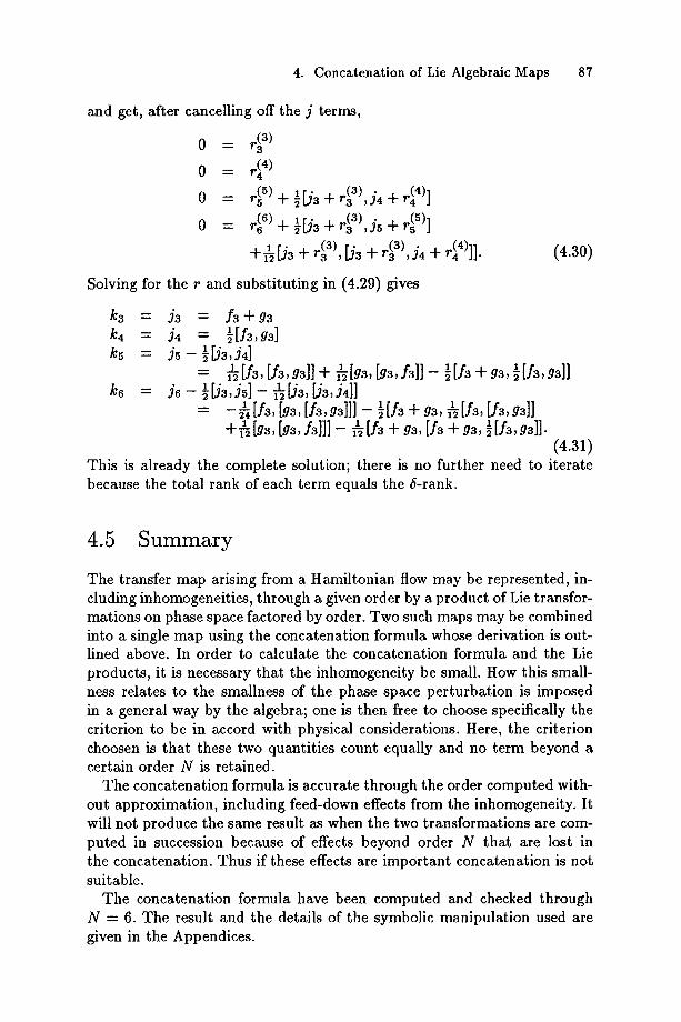
and get, after cancelling off the j terms,

0 = r (3)

0 ---- r l 4)

o = + [j3 + +

+ [J3 + [J3 + 13), J, + r(:)]].

Solving for the r and substituting in (4.29) gives

k3 = J3 = f 3 + g 3 1 k4 -- J4 "- ~[13,g3]

l * • k5 = j5 - ~[J3,J4]

k 6 - -

(4.30)

1 = ~ [1~, [1~, g~]] + ,~[93, [9,, 1~11 - ½11, + g~, ~[ / , , g,]] j6 - ½ [J3, js] - ~ [j3, [i3, J411

= -- ~ [f3, [93, [f3, g31]] -- ½ [f3 "4- g3, ~ [f3, [f3, g3]] 1 -4- ~ [g3, [93, f3]]] -- ~ [f3 -4- 93, [f3 -4- .q3, ~ [f3, g3]].

(4.31) This is already the complete solution; there is no further need to iterate because the total rank of each term equals the 6-rank.

4.5 Summary

The transfer map arising from a Hamiltonian flow may be represented, including inhomogeneities, through a given order by a product of Lie transformations on phase space factored by order. Two such maps may be combined into a single map using the concatenation formula whose derivation is out- lined above. In order to calculate the concatenation formula and the Lie products, it is necessary that the inhomogeneity be small. How this smallness relates to the smallness of the phase space perturbation is imposed in a general way by the algebra; one is then free to choose specifically the criterion to be in accord with physical considerations. Here, the criterion choosen is that these two quantities count equally and no term beyond a certain order N is retained.

The concatenation formula is accurate through the order computed without approximation, including feed-down effects from the inhomogeneity. It will not produce the same result as when the two transformations are computed in succession because of effects beyond order N that are lost in the concatenation. Thus if these effects are important concatenation is not suitable.

The concatenation formula have been computed and checked through N = 6. The result and the details of the symbolic manipulation used are given in the Appendices.


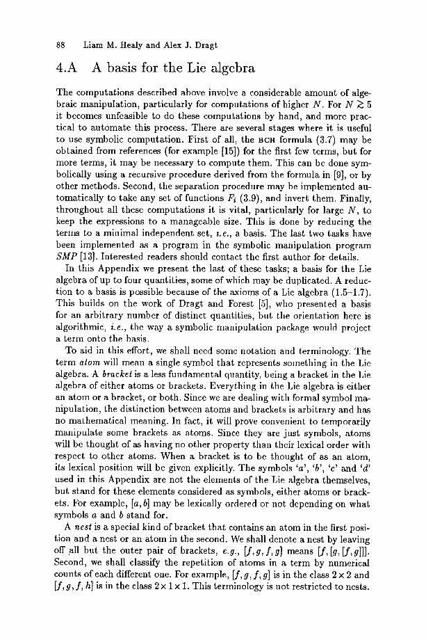
4.A A basis for the Lie algebra

The computations described above involve a considerable amount of algebraic manipulation, particularly for computations of higher N. For N ~ 5 it becomes unfeasible to do these computations by hand, and more practical to automate this process. There are several stages where it is useful to use symbolic computation. First of all, the BCH formula (3.7) may be obtained from references (for example [15]) for the first few terms, but for more terms, it may be necessary to compute them. This can be done symbolically using a recursive procedure derived from the formula in [9], or by other methods. Second, the separation procedure may be implemented au- tomatically to take any set of functions Fi (3.9), and invert them. Finally, throughout all these computations it is vital, particularly for large N, to keep the expressions to a manageable size. This is done by reducing the terms to a minimal independent set, z.e., a basis. The last two tasks have been implemented as a program in the symbolic manipulation program SMP [13]. Interested readers should contact the first author for details.

In this Appendix we present the last of these tasks; a basis for the Lie algebra of up to four quantities, some of which may be duplicated. A reduc- tion to a basis is possible because of the axioms of a Lie algebra (1.5-1.7). This builds on the work of Dragt and Forest [5], who presented a basis for an arbitrary number of distinct quantities, but the orientation here is algorithmic, i.e., the way a symbolic manipulation package would project a term onto the basis.

To aid in this effort, we shall need some notation and terminology. The term atom will mean a single symbol that represents something in the Lie algebra. A bracket is a less fundamental quantity, being a bracket in the Lie algebra of either atoms or brackets. Everything in the Lie algebra is either an atom or a bracket, or both. Since we are dealing with formal symbol manipulation, the distinction between atoms and brackets is arbitrary and has no mathematical meaning. In fact, it will prove convenient to temporarily manipulate some brackets as atoms. Since they are just symbols, atoms will be thought of as having no other property than their lexical order with respect to other atoms. When a bracket is to be thought of as an atom, its lexical position will be given explicitly. The symbols 'a', 'b', 'c' and 'd' used in this Appendix are not the elements of the Lie algebra themselves, but stand for these elements considered as symbols, either atoms or brackets. For example, [a, b] may be lexically ordered or not depending on what symbols a and b stand for.

A nest is a special kind of bracket that contains an atom in the first position and a nest or an atom in the second. We shall denote a nest by leaving off all but the outer pair of brackets, e.g., [f,g, f ,g] means [f, [g, [f,g]]]. Second, we shall classify the repetition of atoms in a term by numerical counts of each different one. For example, [f, g, f , g] is in the class 2 x 2 and [f, g, f , h] is in the class 2 × 1 × 1. This terminology is not restricted to nests.


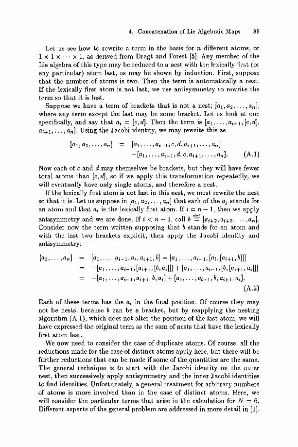
Let us see how to rewrite a te rm in the basis for n different atoms, or 1 x 1 x - . . x 1, as derived from Dragt and Forest [5]. Any member of the Lie algebra of this type may be reduced to a nest with the lexically first (or any part icular) a tom last, as may be shown by induction. First, suppose tha t the number of atoms is two. Then the term is automatical ly a nest. If the lexically first a tom is not last, we use an t i symmetry to rewrite the te rm so tha t it is last.

Suppose we have a term of brackets tha t is not a nest; [a],a2,... ,an], where any te rm except the last may be some bracket. Let us look at one specifically, and say tha t a, = [c, d]. Then the te rm is [ a l , . . . , a i - t , [c, d], ai+t , . . . , an]. Using the Jacobi identity, we may rewrite this as

[at,a2,...,a,~] - [a t , . . . ,a i_ l ,c ,d , a i+l , . . . ,a ,] - [a l , . . . ,a,_t,d,c, ai+x,... ,an]. (A.1)

Now each of c and d may themselves be brackets, but they will have fewer total a toms than [c, d], so if we apply this t ransformation repeatedly, we will eventually have only single atoms, and therefore a nest.

If the lexically first a tom is not last in this nest, we must rewrite the nest so tha t it is. Let us suppose in [al,a2,.. . ,an] tha t each of the a~ s tands for an a tom and tha t ai is the lexically first atom. If i = n - 1, then we apply

def an t i symmet ry and we are done. If i < n - 1, call b = [ai+2, ai+3,... ,an]. Consider now the te rm writ ten supposing tha.t b s tands for an a tom and with the last two brackets explicit; then apply the Jacobi identi ty and ant isymmetry:

an] = [ a t , . . . , ai_ , a,, b] = Ca1, . . . , [a i+l , b]]] = ai_ , [b, a,]]] + [b, a,]]]

= - - [ a l , . . . , a i - l , a i + l , b, ai] -4- [ a l , . . . , a i _ l , b , ai+l,ai]. (A.2)

Each of these terms has the ai in the final position. Of course they may not be nests, because b can be a bracket, but by reapplying the nesting algori thm (A.1), which does not alter the position of the last atom, we will have expressed the original te rm as the sum of nests tha t have the lexically first a tom last.

We now need to consider the case of duplicate atoms. Of course, all the reductions made for the case of distinct a toms apply here, but there will be further reductions tha t can be made if some of the quantities are the same. The general technique is to s tar t with the Jacobi identi ty on the outer nest, then successively apply an t i symmet ry and the inner Jacobi identities to find identities. Unfortunately, a general t rea tment for arbi t rary numbers of atoms is more involved than in the case of distinct atoms. Here, we will consider the particular terms tha t arise in the calculation for N = 6. Different aspects of the general problem are addressed in more detail in [1].


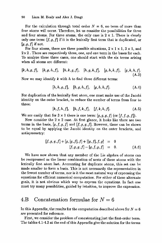
For the calculation through total order N = 6, no term of more than four atoms will occur. Therefore, let us consider the possibilities for three and four atoms. For three atoms, the only case is 2 x 1. There is clearly only one term: [f, g, f] if it is the lexically first term that is duplicated, or [g , g, f] if not.

For four atoms, there are three possible situations, 2 x 1 x 1, 3 x 1, and 2 x 2. There are respectively three, one, and one term in the bases for each. To analyze these three cases, one should start with the six terms arising when all atoms are different:

[k,h,g,f], [k,g,h,f], [h,k,g,f], [h,g,k,f], [#,h,k,f],

Now we may identify k with h to find three different terms:

[h,h,g,f], [h,g,h,f], [g,h,h,f].

[g, k, h, f]. (A.3)

(A.4)

For duplication of the lexically first atom, one must make use of the Jacobi identity on the outer bracket, to reduce the number of terms from four to three:

[k, f ,h , f] , [h, f ,k , f] , [ f ,k ,h, f] . (A.5)

We see easily that for 3 x 1 there is one term: [g, g, g, f] (or [f, f , g, f]). Now consider the 2 x 2 case. At first glance, it looks like there are two

terms in the basis, [g, f , g, f] and [f, g, g, f] . However, these can be shown to be equal by applying the Ja~obi identity on the outer brackets, and antisymmetry:

[ f ,g ,g , f ]+[g , [g , f ] , f ]+ [[g,f],f,g] = 0 [ f , g , g , f ] - [g,f ,g,f] = O. (A.6)

We have now shown that any member of the Lie algebra of atoms can be reexpressed as the linear combination of nests of these atoms with the lexically first atom last. Accounting for duplicate atoms, this set can be made smaller to form a basis. This is not necessarily the representation in the fewest number of terms, nor is it the most natural way of expressing the equations for efficient numerical computation. For either of these alternate goals, it is not obvious which way to express the equations. In fact one must try many possiblities, guided by intuition, to improve the expression.

4 .B C o n c a t e n a t i o n f o r m u l a e for N - 6

In this Appendix, the results for the computation described above for N = 6 are presented for reference.

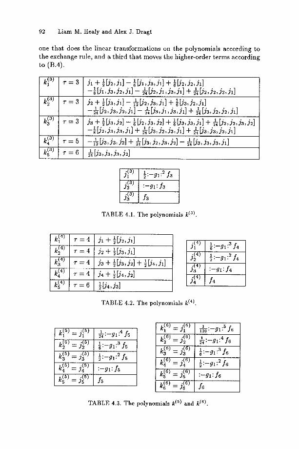
First, we consider the problem of concatenating just the first-order term. The tables 4.1-4.3 at the end of this Appendix give the solution for the terms


on the right side of (4.11). In these tables, the k are described in terms of j . Since these j always have the same superscript as the k, it has been left off. Note in the tables the manifestation of the condition determining the number of brackets required (3.10): for the k (3) expressions, there are at most 3 brackets in a term, for the k (4) calculations, at most 1, and for k (5) and k(6), no brackets. The expressions for k may be obtained from Appendix 4.C by keeping only these number of brackets and setting the appropriate j to zero.

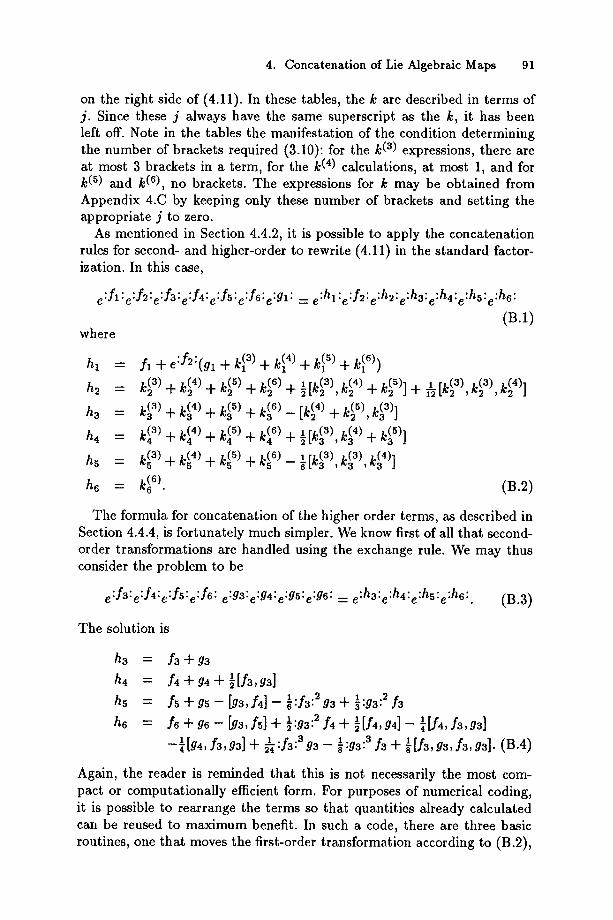
As mentioned in Section 4.4.2, it is possible to apply the concatenation rules for second- and higher-order to rewrite (4.11) in the standard factorization. In this case,

e:fZ:e:f2:e:fZ:e:f4:e:fh:e:f6:e:gl: = e:hl:e:f2:e:h2:e:h3:e:h4:e:hh:e:h6: (B.1)

where

hl = f l q- e:f2:(gl -t- k~ 3) q- k~ 4) -I- k~ 5) -}" k~ 6)) : z r/,.(3) /.(4) rt.(3) t.(3) h= k~ :~ + k~ 4~ + k~ °~ + k~ °~ + ~,.~ , .~ + k ~ l + ~ ~ , .~ , k~4>l

_ k ( 5 ) k ( 3 ) 1 h~ = g3) + g , ) + g~) + go) tk~") + ~ , ~. , = ~rb(3) /,.(4) h, k, ~ + k~"~ + k,~'~ + k ~ + ~,.~ , ~ + ~?~]

h~ : k~ ~ + ~ ' ~ + ~ + k~ °~ - ~[g3~, k¢~:3 , ¢'~:3 ,

h~ = k~ 6~. (n.2)

The formula for concatenation of the higher order terms, as described in Section 4.4.4, is fortunately much simpler. We know first of all that second- order transformations are handled using the exchange rule. We may thus consider the problem to be

e:fa:e:f4:e:fh:e :f6: e:g3:e:g4:e:gh:e :g6: : e:ha:e:h4:e:h~:e :h6:. (B.3)

The solution is

h3 = f 3 + g 3

h~ = f~ + g~ + ½[f~, g~] __ 1 . 2 hs = Ys+g5 [g3,f4]-}:f3:2ga+~.g3: Y3

1. 2 ' [f4, g4] -- ¼ [f4, f3, g31 h6 = f6 "4- g6 - [g3, fs] "4- ~ .g3: f4 q- z "f3"3 z -¼[g4 , f3 ,g~ ] + ~ . • g 3 - ~:g3:3 f~ + ~[ f3 ,g3 , f~ ,g3] . (B.4)

Again, the reader is reminded that this is not necessarily the most com- pact or computationally efficient form. For purposes of numerical coding, it is possible to rearrange the terms so that quantities already calculated can be reused to maximum benefit. In such a code, there are three basic routines, one that moves the first-order transformation according to (B.2),


one that does the linear transformations on the polynomials according to the exchange rule, and a third that moves the higher-order terms according to (B.4).

1 ° ° • k~ 3) 7" = 3 j~ + l [ j~ , j~]_ ~[Jl,j3,j~] + g[J2,Y2,)~] 1 . . . . -~[ .h ,~a , J~,.h] - ~ ~D~, ) I , ) a ,y~] + ~b~,g2,Yu,J l ]

k~ 3) 7 " - 3 J2+ ½[J3 , J~] -~[ j : , Ja , j l ]+ ~ " " "~[j3,y2,)~] - ~ [J~, J~, J~, J~] - ~ b~, ~1, ~ , ~] + ~ b~, ~, ~ , J~]

k(33) r = 3 j 3 + ½ [ J 3 , j 2 ] - ' ' " " 1 • • • [ J 2 , 3 3 , 3 2 ] J v ~ [ J 3 , 3 3 , 3 1 ] "~- 1 [j2, j~, j3, j~] 1 . . . . - ~ [ ~ , ~ , ~ , ~ x ] + ~ [ ~ , ~ , ~ , ~ , ] + 5 b ~ , ~ , ~ , ~ x ]

k (3) 7" - 5 ' 1 • • • 1 . . . . 1 . . . . . -~[J3,33,32] + ~[j3,32,33,j2]- ~[J3,33,33,3~] k~ 3) r = 6 ' ~ [ j 3 , j a , j a , j 2 ]

$.--g1:2 f3

5~ 3) : - g l : f3

j(33) f3

TABLE 4.1. The polynomials k (3).

k~ 4) k~ 4)

k(3 4)

k( 4 )

k~ 4)

r = 4

v = 4

7 = 4

7 " = 4

v = 6

j l + 1[j2, j l]

J~ + ½D3, j l]

j 3 + 71 [J3, j2] + 51 [j4, j l] 1 " j4 -~- ~ [j4, j2]

½ [j4, J3]

j~4)

j~4)

5(34)

5 (4)

TABLE 4.2. The polynomials k (4).

1 . 3 ~ . - g l : f4 1 2 i : - -gl : f4

:--gl: f4

f4

k?)= 5)

k(35)= 5(35)

k(:) = 5(:) k~5)= 5~ 5)

1 . 4 ~ . - g l : f5

:-g1:3 A l:_g 1:2 A

: - g l : f5

k~6)= j~6) 6)

k(36)= 5(36)

= S : k~S) = 5~ 6) k~6)= 5~ 6)

,~0 :-g1:5 f6 l : - - g l : 4 f6

:-g1:3 f6

½ :-g1:2 f6 : - g l : f6

TABLE 4.3. The polynomials k (5) and k (6).

4.C T h e r e su l t s N = 6

4. Concatenation of Lie Algebraic Maps

of the s e p a r a t i o n p r o c e d u r e for

93

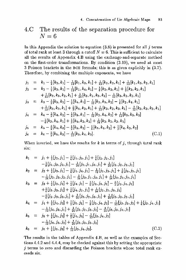
In this Append ix the solut ion to equat ion (3.8) is presented for all j t e rms of total rank at least 3 th rough a cutoff N = 6. This is sufficient to calculate all the results of Append ix 4.B using the exchange-and-separa te m e t h o d on the first-order t ransformat ions . By condi t ion (3.10), we need at mos t 3 Poisson brackets in the BCH formula; this is as given explicitly in (3.7). Therefore, by combining the mul t ip le exponents , we have

j l "-- k l - ½ [ k 2 , k l ] - 1-~ [k l , k3, k l ] "4- ~ [k2, k2, k l ] -~" ?~ [k l , k3, k2, k l ] j~ = k ~ - }[k~,~a]- ~[k~,k~,k~]-I

+~[~, ~ , ~ , ~] + ~[~, ~1, ~, ~11- ~[~, ~, ~, ~] jz = kz - ½[k3, k~] - ½[k4, kl] - ~[k2, k3, k~] - ~[k~, k4, k~]

+~[~, ~, ~] + }[~,, ~, ~1] + ~[~, ~, ~, ~,]- ~[~, ~, ~, ~1] 1 j4 = k 4 - ½[k4, k ~ ] - g[ks, k~]- ~[k~,k4, k2] + ~[k3 ,ka , k~]

1 1 -~[~, ~,, ~] + ~[~,, ~, ~] + ~[~, ~, ~, ~] j~ = ~ _ 1[~,,~]_ ½[~,~]_ }[~,~,,~] + }[~,,~,~]

j6 = k6 - ½[ks , ka ] - l~[k3,k4, k3]. (C.1)

When inverted, we have the results for k in te rms of j , th rough total rank s ix :

1 • 1 [ i l , J3, Jl] + 1 [ j~ , J2, Jl] kl = Jl -t- ~ [ J 2 , J l ] - g g

-~[ j l , ja , j2 , j l ] - ~[j2,jl , ja,jl] + ~[j2,j2,j2,jl] 1 • l ~ / 1 , j 4 , j l ] - ~[j2,j3,jl] + k2 = j2 + 7[Ja, j l] - g l [ Ja , j2 , j l ]

- ~ [J2, J3, J2, Jl] - ~ [J3, J~, J3, J~] + ~ [Ja, J2, J2, J~] ~ . 1 • 1 [J4, j l ] -- "i[32' j3, j2] -- 1 " k3 j3 + 7[Ja,j2] + g 1 • g[Y2,j4,jl]

+ ~ [ j 3 , j a , j l ] + ~[ ja , j2 , j l ] + ~[J2,j2,J3,j2] 1 . . . . 1 . . . .

-~[J2,Y3,aa,31] + ~[aa,Y2,23,31] + ~[j3,Ja,J2,Jl] k4 = j4 + 1 • 1 • 1 [ j3 , j4 , j l ] [Y2, j4, j21 - ~ [j3, j3, j2] + ~[j~,j~] ~ [J4, j2] +

~2[J4,ja,Jl] + ~[J3,j2,ja,j2] - ~[j3,j3,ja,jl] 1 " 1 " 1 " k~ = j5 + ~[J~,J2] + i[J4,j3] - ~[y3, j4, j2]

i~2 [J4, ja, j2] + ~ [j3, ja, j3, j2] 1 • 1 " 1:6 ---- j6 + ~[Js,j3] + i~[J3, j4,j3]. (C.2)

The results in the tables of Append ix 4.B, as well as the examples of Sec- t ions 4.4.2 and 4.4.4, may be checked against this by set t ing the appropr ia te j te rms to zero and discarding the Poisson brackets whose total rank exceeds six.


4.6 Acknowledgements

This paper is based on the dissertation [10] of one of the authors. We would also like to thank the Inference Corporation, who provided much assistance in understanding and applying SMP. This work was supported by U.S. Department of Energy contract number DE-AS05-80ER-10666.

4 .7 REFERENCES

[1] N. Bourbaki, Elements of Mathematics, Lie Groups and Lie Algebras (Addison-Wesley, Reading, Massachusetts, 1971); Part I: Chapters 1- 3.

[2] D. R. Douglas, Ph.D. dissertation, University of Maryland Physics Department Technical Report (1982).

[3] A.J. Dragt, Lectures on Nonlinear Orbit Dynamics, in: Physics of Hzgh Energy Partzcle Accelerators, Proceedings of the 1981 Summer School on High Energy Particle Accelerators, New York, R.A. Carrigan, F.R. Huson, and M. Month, eds., American Institute of Physics, Conference Proceedings Number 87, 1982, p. 147.

[4] A.J. Dragt, and J.M. Finn, Lie series and invariant functions for analytic symplectic maps, 3. Math. Phys. 17, 2215 (1976).

[5] A.J. Dragt, and E. Forest, Computation of nonlinear behavior of Hamiltonian systems using Lie algebraic methods, 3. Math. Phys. 24, 2734 (1983).

[6] A.J. Dragt et al., MAl~YLIE 3.0 manual, University of Maryland Tech- nical Report (1988).

[7] A.J. Dragt, L.M. Healy, F.Neri, R.D. Ryne, D.R. Douglas, and E.Forest, MARYLIE 3.0 --A Program for Nonlinear Analysis of Accel- erators and Beamline Lattices, IEEE Trans. Nucl. Sci. NS-32, 2311 (1985).

[8] A.J. Dragt, F. Neri, G. Rangarajan, D. Douglas, L.M. Healy, and R.D. Ryne, Lie algebraic treatment of linear and nonlinear beam dynamics, Ann. Rev. Nucl. Part. Sci. 38,455-496 (1988).

[9] M. Hausner and J. Schwartz, Lie Groups Lie Algebras (Gordon and Breach, New York, 1968).

[10] L.M. Healy, Ph.D. dissertation, University of Maryland Physics De- partment Technical Report (1986).


[11]

[12]

[13]

[14]

[15]

L.M. Healy and A.J. Dragt, Lie algebraic methods for treating lattice parameter errors in accelerators. In: Proceedings of the 1987 IEEE Particle Accelerator Conference Vol. 2, (1987), p. 1060 et seq.

L.M. Healy and A.J. Dragt, Computation of nonlinear behavior of inhomogeneous ttamiltonian systems using Lie algebraic methods (in preparation).

SMP Manual, Inference Corporation, 1985.

F.J. Murray and K.S. Miller, Ezistence Theorems (New York Univer- sity Press, New York, 1954).

V.S. Varadarajan, Lie Groups, Lie Algebras, and their Representations (Springer-Verlag, New York, 1984).

Concatenation of Lie algebraic maps

Documents