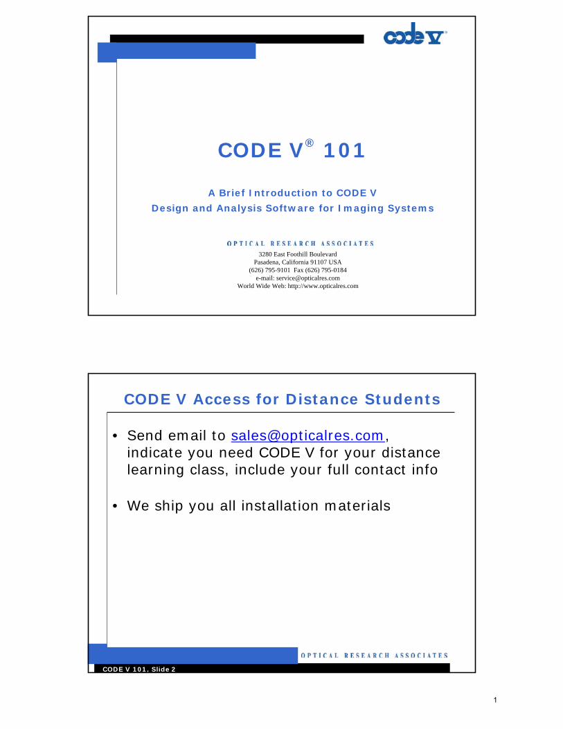
3280 East Foothill Boulevard Pasadena, California 91107 USA (626) 795-9101 Fax (626) 795-0184 e-mail: [email protected] World Wide Web: http://www.opticalres.com CODE V ® 101 A Brief Introduction to CODE V Design and Analysis Software for Imaging Systems CODE V 101, Slide 2 CODE V Access for Distance Students • Send email to [email protected] , indicate you need CODE V for your distance learning class, include your full contact info • We ship you all installation materials 1

Welcome message from author
This document is posted to help you gain knowledge. Please leave a comment to let me know what you think about it! Share it to your friends and learn new things together.
Transcript
1
3280 East Foothill BoulevardPasadena, California 91107 USA
(626) 795-9101 Fax (626) 795-0184e-mail: [email protected]
World Wide Web: http://www.opticalres.com
CODE V® 101
A Brief Introduction to CODE V
Design and Analysis Software for Imaging Systems
CODE V 101, Slide 2
CODE V Access for Distance Students
• Send email to [email protected], indicate you need CODE V for your distance learning class, include your full contact info
• We ship you all installation materials
1
2
CODE V 101, Slide 3
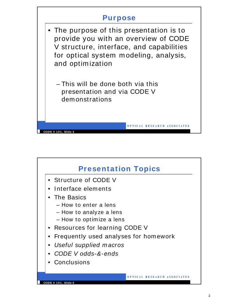
Purpose
• The purpose of this presentation is to provide you with an overview of CODE V structure, interface, and capabilities for optical system modeling, analysis, and optimization
–This will be done both via this presentation and via CODE V demonstrations
CODE V 101, Slide 4
Presentation Topics• Structure of CODE V• Interface elements• The Basics
– How to enter a lens– How to analyze a lens– How to optimize a lens
• Resources for learning CODE V• Frequently used analyses for homework• Useful supplied macros• CODE V odds-&-ends• Conclusions
2
3
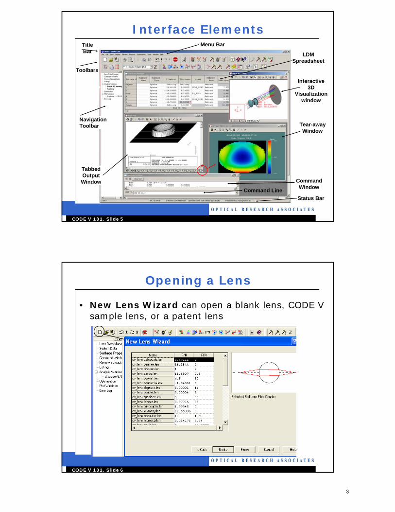
CODE V 101, Slide 5
Interface ElementsTitle Bar
Navigation Toolbar
Menu Bar
Toolbars
LDM Spreadsheet
Command Window
Command Line
Tear-away Window
Status Bar
Tabbed Output
Window
Interactive 3D
Visualization window
CODE V 101, Slide 6
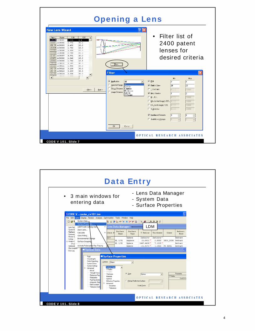
Opening a Lens
• New Lens Wizard can open a blank lens, CODE V sample lens, or a patent lens
3
4
CODE V 101, Slide 7
Opening a Lens
• Filter list of 2400 patent lenses for desired criteria
CODE V 101, Slide 8
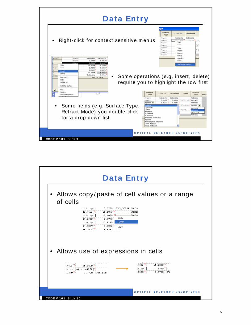
Data Entry
LDM
• 3 main windows for entering data
- Lens Data Manager- System Data- Surface Properties
4
5
CODE V 101, Slide 9
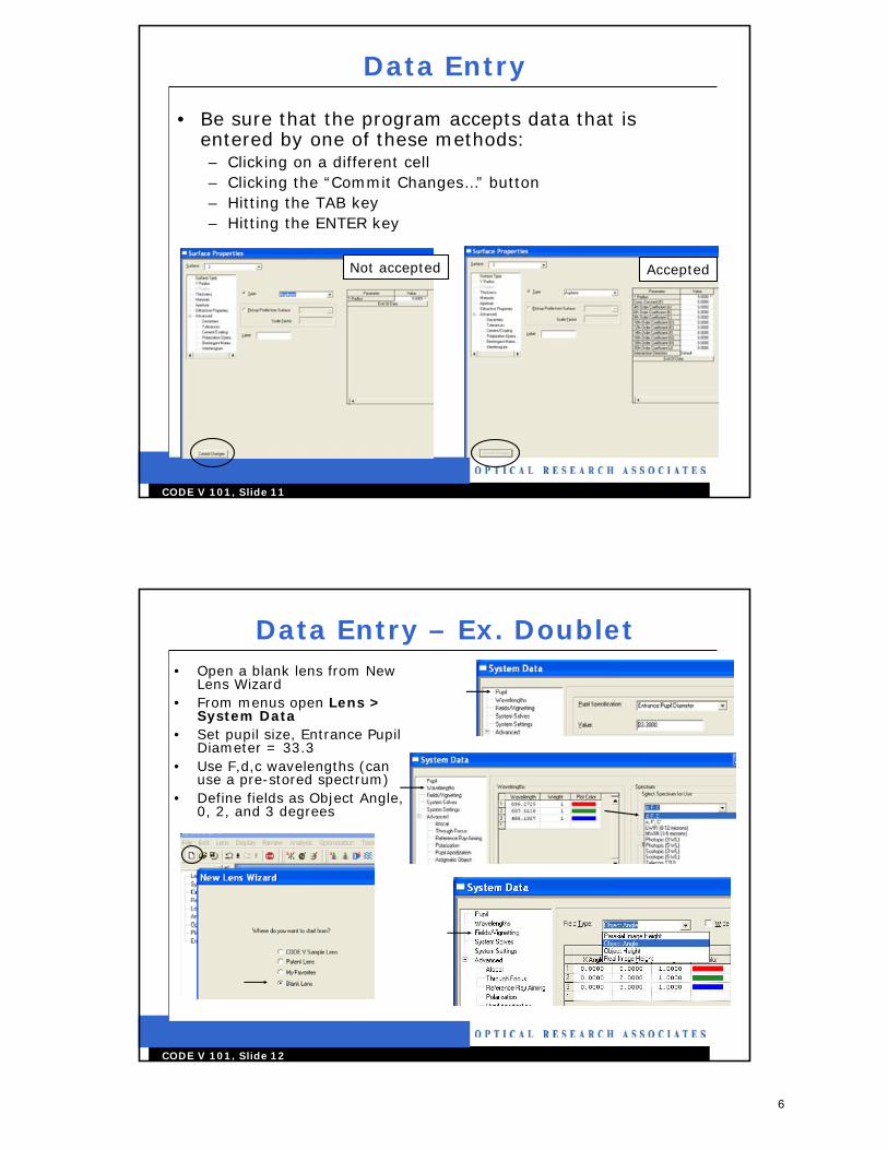
Data Entry
• Right-click for context sensitive menus
• Some operations (e.g. insert, delete) require you to highlight the row first
• Some fields (e.g. Surface Type, Refract Mode) you double-click for a drop down list
CODE V 101, Slide 10
Data Entry
• Allows copy/paste of cell values or a range of cells
• Allows use of expressions in cells
5
6
CODE V 101, Slide 11
Data Entry
• Be sure that the program accepts data that is entered by one of these methods:– Clicking on a different cell– Clicking the “Commit Changes…” button– Hitting the TAB key– Hitting the ENTER key
Not accepted Accepted
CODE V 101, Slide 12
Data Entry – Ex. Doublet• Open a blank lens from New
Lens Wizard• From menus open Lens >
System Data• Set pupil size, Entrance Pupil
Diameter = 33.3• Use F,d,c wavelengths (can
use a pre-stored spectrum)• Define fields as Object Angle,
0, 2, and 3 degrees
6
7
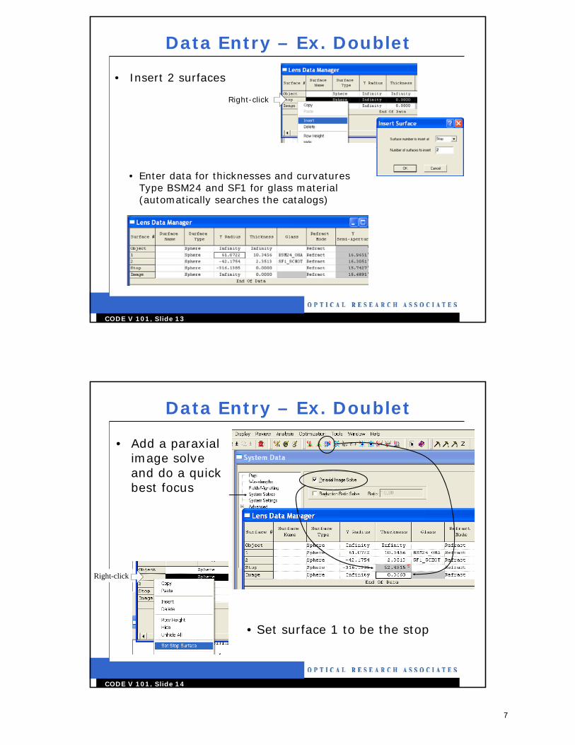
CODE V 101, Slide 13
Data Entry – Ex. Doublet
• Insert 2 surfaces
Right-click
• Enter data for thicknesses and curvaturesType BSM24 and SF1 for glass material (automatically searches the catalogs)
CODE V 101, Slide 14
Data Entry – Ex. Doublet
• Add a paraxial image solve and do a quick best focus
• Set surface 1 to be the stop
Right-click
7
8
CODE V 101, Slide 15
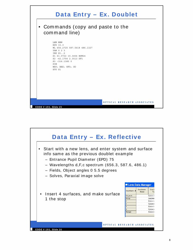
Data Entry – Ex. Doublet
• Commands (copy and paste to the command line)
LEN NEWEPD 33.3WL 656.2725 587.5618 486.1327YAN 0 2 3 INS S1..2S1 61.0722 10.3456 BSM24S2 -42.1754 2.3513 SF1S3 -316.1385 0 PIMWAV; BES; RFO; GOSTO S1
CODE V 101, Slide 16
Data Entry – Ex. Reflective
• Start with a new lens, and enter system and surface info same as the previous doublet example– Entrance Pupil Diameter (EPD) 75– Wavelengths d,F,c spectrum (656.3, 587.6, 486.1)– Fields, Object angles 0 5.5 degrees– Solves, Paraxial image solve
• Insert 4 surfaces, and make surface 1 the stop
8
9
CODE V 101, Slide 17
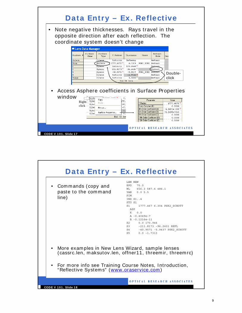
Data Entry – Ex. Reflective• Note negative thicknesses. Rays travel in the
opposite direction after each reflection. The coordinate system doesn’t change
• Access Asphere coefficients in Surface Properties window
Double-click
Right-click
CODE V 101, Slide 18
Data Entry – Ex. Reflective
• Commands (copy and paste to the command line)
LEN NEWEPD 75.0WL 656.3 587.6 486.1YAN 0.0 5.5PIMINS S1..4STO S1S1 1777.467 6.304 PSK2_SCHOTT
ASPK 0.0A -0.4049e-7B -0.1216e-11
S2 0.0 170.946S3 -211.8173 -96.2601 REFLS4 -40.9571 -5.9437 PSK2_SCHOTTS5 0.0 -1.7313
• More examples in New Lens Wizard, sample lenses (cassrc.len, maksutov.len, offner11, threemir, threemrc)
• For more info see Training Course Notes, Introduction, “Reflective Systems” (www.oraservice.com)
9
10
CODE V 101, Slide 19
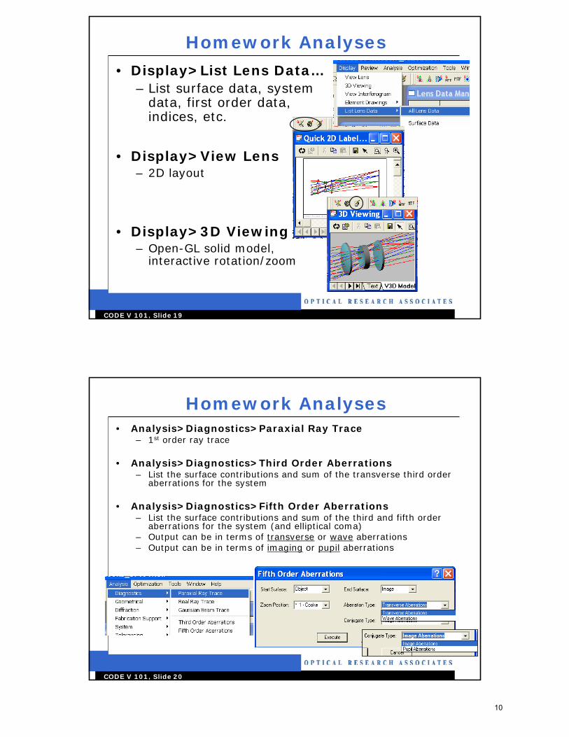
Homework Analyses
• Display>List Lens Data…– List surface data, system
data, first order data, indices, etc.
• Display>View Lens– 2D layout
• Display>3D Viewing– Open-GL solid model,
interactive rotation/zoom
CODE V 101, Slide 20
Homework Analyses• Analysis>Diagnostics>Paraxial Ray Trace
– 1st order ray trace
• Analysis>Diagnostics>Third Order Aberrations– List the surface contributions and sum of the transverse third order
aberrations for the system
• Analysis>Diagnostics>Fifth Order Aberrations– List the surface contributions and sum of the third and fifth order
aberrations for the system (and elliptical coma)– Output can be in terms of transverse or wave aberrations– Output can be in terms of imaging or pupil aberrations
10
11
CODE V 101, Slide 21
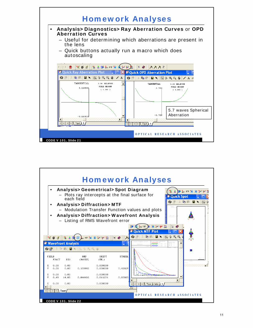
Homework Analyses• Analysis>Diagnostics>Ray Aberration Curves or OPD
Aberration Curves– Useful for determining which aberrations are present in
the lens– Quick buttons actually run a macro which does
autoscaling
5.7 waves Spherical Aberration
CODE V 101, Slide 22
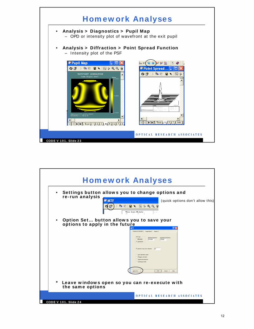
Homework Analyses• Analysis>Geometrical>Spot Diagram
– Plots ray intercepts at the final surface for each field
• Analysis>Diffraction>MTF– Modulation Transfer Function values and plots
• Analysis>Diffraction>Wavefront Analysis– Listing of RMS Wavefront error
11
12
CODE V 101, Slide 23
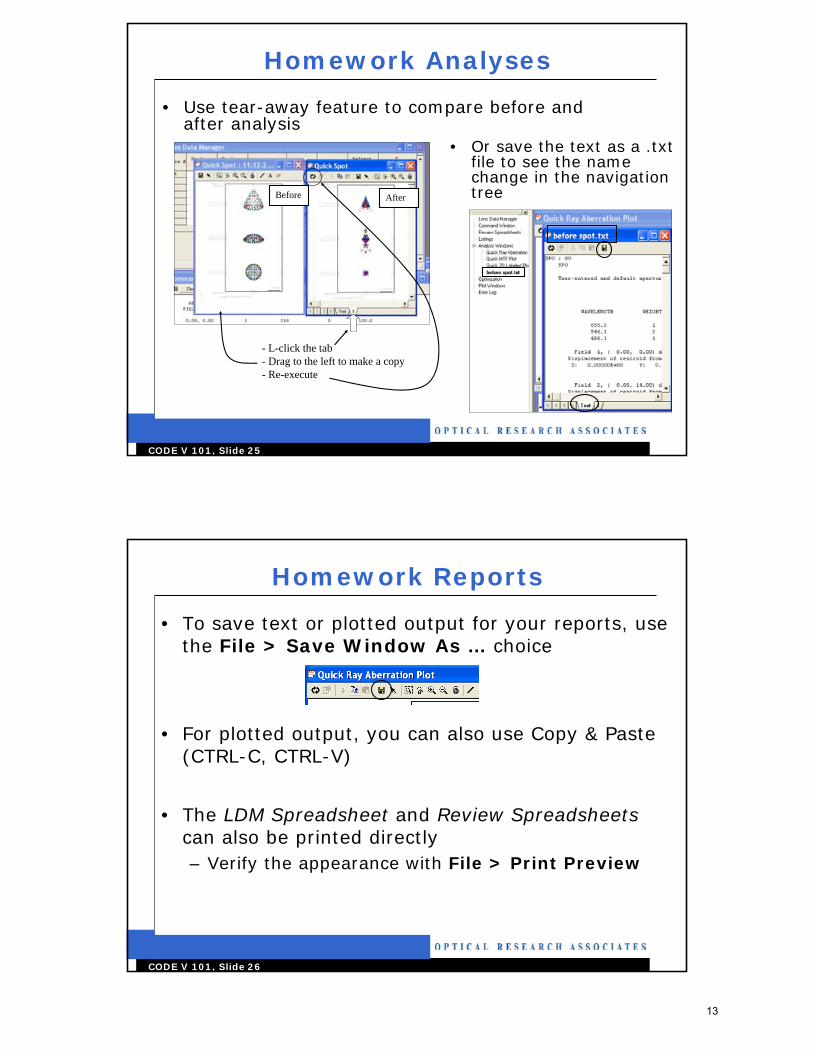
Homework Analyses• Analysis > Diagnostics > Pupil Map
– OPD or intensity plot of wavefront at the exit pupil
• Analysis > Diffraction > Point Spread Function– Intensity plot of the PSF
CODE V 101, Slide 24
Homework Analyses• Settings button allows you to change options and
re-run analysis
• Option Set… button allows you to save your options to apply in the future
* Leave windows open so you can re-execute with the same options
(quick options don’t allow this)
12
13
CODE V 101, Slide 25
Homework Analyses
• Use tear-away feature to compare before and after analysis
• Or save the text as a .txt file to see the name change in the navigation tree
- L-click the tab- Drag to the left to make a copy- Re-execute
Before After
CODE V 101, Slide 26
Homework Reports
• To save text or plotted output for your reports, use the File > Save Window As … choice
• For plotted output, you can also use Copy & Paste (CTRL-C, CTRL-V)
• The LDM Spreadsheet and Review Spreadsheetscan also be printed directly– Verify the appearance with File > Print Preview
13
14
CODE V 101, Slide 27
Demo – Setup Lens
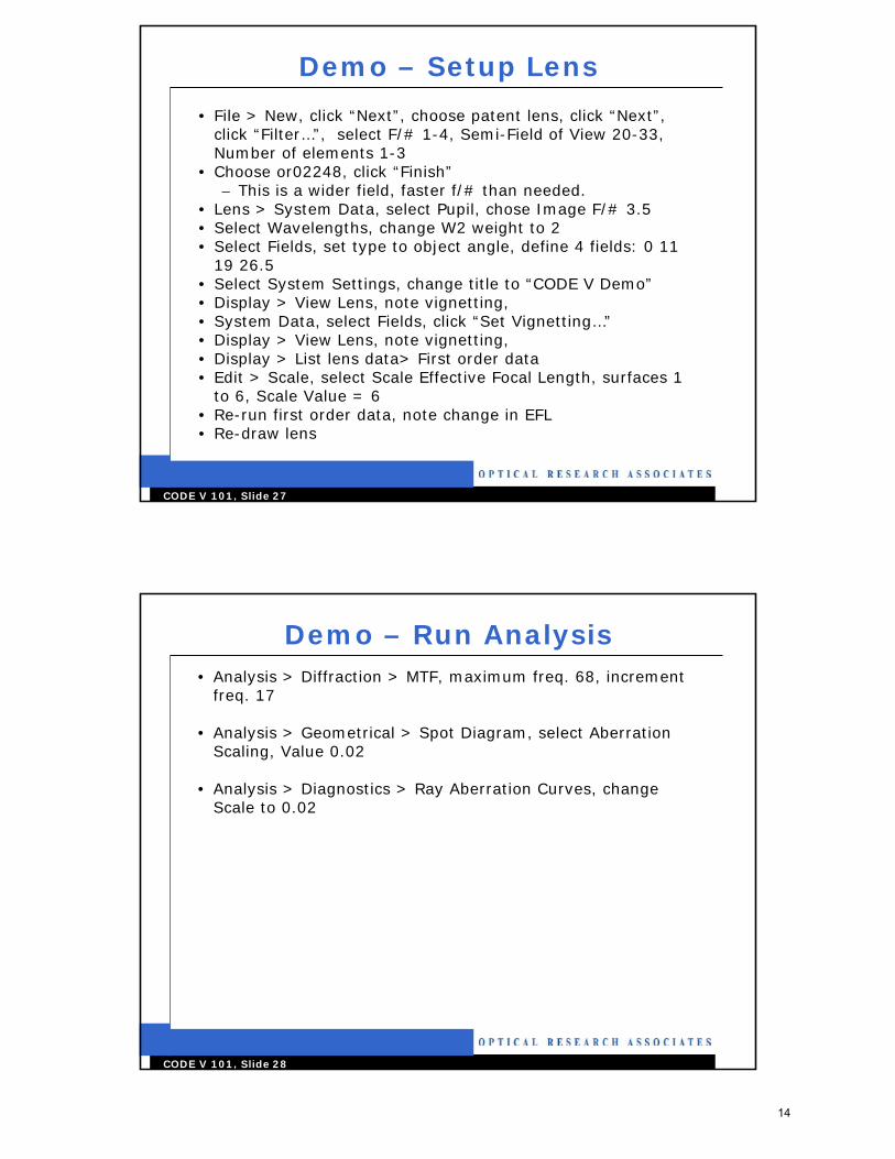
• File > New, click “Next”, choose patent lens, click “Next”, click “Filter…”, select F/# 1-4, Semi-Field of View 20-33, Number of elements 1-3
• Choose or02248, click “Finish”– This is a wider field, faster f/# than needed.
• Lens > System Data, select Pupil, chose Image F/# 3.5• Select Wavelengths, change W2 weight to 2• Select Fields, set type to object angle, define 4 fields: 0 11
19 26.5• Select System Settings, change title to “CODE V Demo”• Display > View Lens, note vignetting, • System Data, select Fields, click “Set Vignetting…”• Display > View Lens, note vignetting, • Display > List lens data> First order data• Edit > Scale, select Scale Effective Focal Length, surfaces 1
to 6, Scale Value = 6• Re-run first order data, note change in EFL• Re-draw lens
CODE V 101, Slide 28
Demo – Run Analysis• Analysis > Diffraction > MTF, maximum freq. 68, increment
freq. 17
• Analysis > Geometrical > Spot Diagram, select Aberration Scaling, Value 0.02
• Analysis > Diagnostics > Ray Aberration Curves, change Scale to 0.02
14
15
CODE V 101, Slide 29
Optimizing a Lens
• One of CODE V’s main strengths is the effectiveness of its optimization algorithms– In particular, CODE V’s ability to control constraints
exactly works better than any other commercial software
• CODE V optimization is easy to use, with very little input required by you in many cases– This is mainly achieved through CODE V’s use of
intelligent defaults– However, the Automatic Design feature is also flexible
and you can control many details of the optimization if you wish to
CODE V 101, Slide 30
Optimizing a Lens
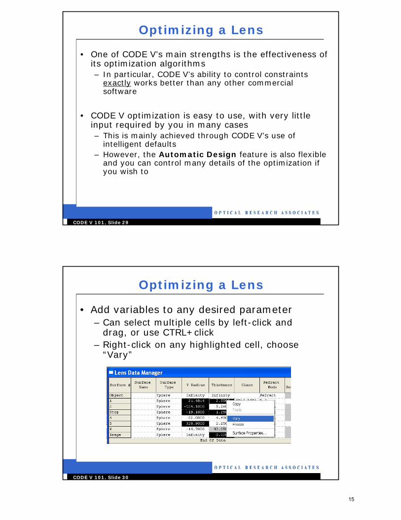
• Add variables to any desired parameter– Can select multiple cells by left-click and
drag, or use CTRL+click– Right-click on any highlighted cell, choose
“Vary”
15
16
CODE V 101, Slide 31
Optimizing a Lens
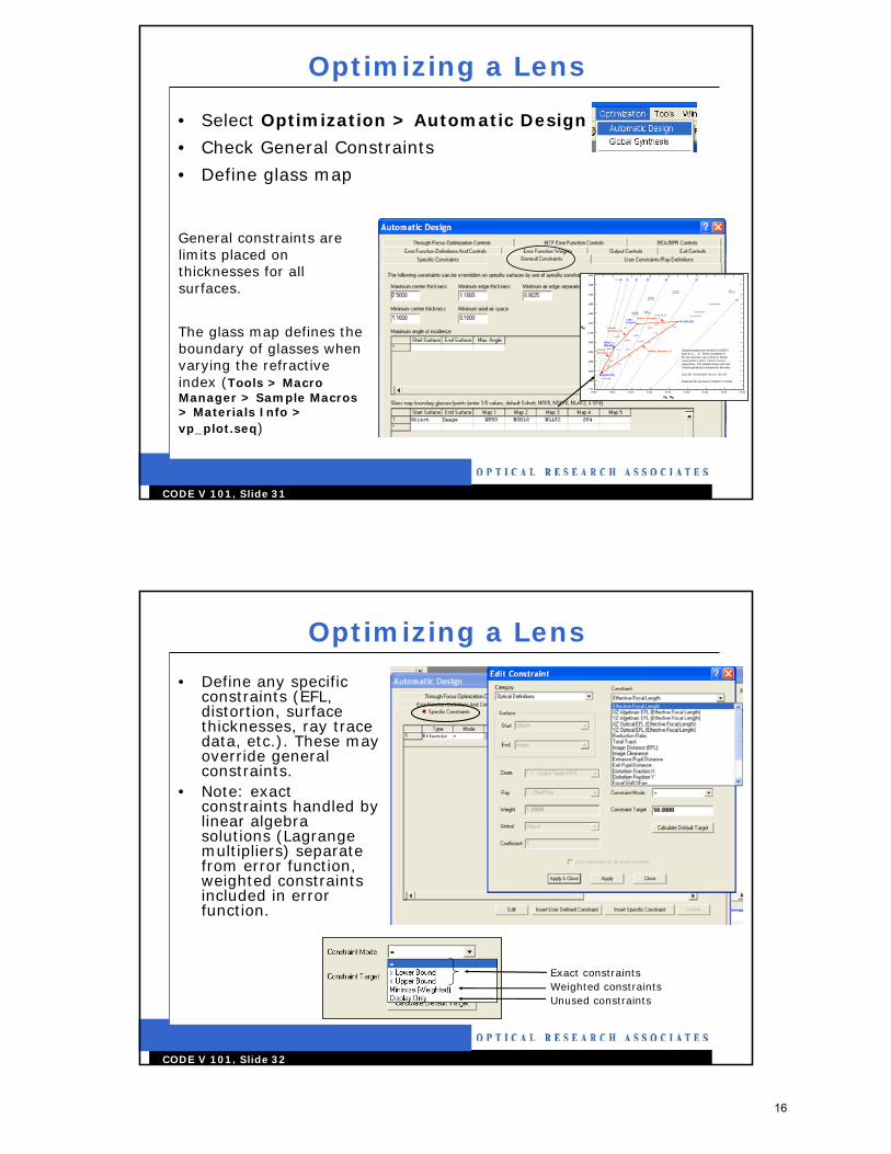
• Select Optimization > Automatic Design
• Check General Constraints
• Define glass map
General constraints are limits placed on thicknesses for all surfaces.
The glass map defines the boundary of glasses when varying the refractive index (Tools > Macro Manager > Sample Macros > Materials Info > vp_plot.seq)
0.005 0.010 0.015 0.020 0.025 0.030 0.035 0.040 0.045
1.50
1.55
1.60
1.65
1.70
1.75
1.80
1.85
1.90
1.95
2.00
1.45
1.40
BK7LLF6
PSK3
LF7
F5SK2 BaF52
BaF50
BaSF10SSKN5
LaKN12
BaSF51
SF2
SF8
SF10
LaFN7
Fused silica
LaK8
LaSFN31(881.410)
LaSFN18(913.324)
SF58(918.215)
SF11 (785.258)
SF6 (805.254)
SF57 (847.238)
LaF22A (782.372)
LaSFN30(803.464)
LaSF3(808.406)
SF4 (755.276)
FK5 (487.704)
LaF2(744.447)
SK16(620.603)
Default Boundary D Glass boundaries are denoted in CODE Vas A, B, C, ..., E. These correspond tothe lines between user-entered or defaultcorner points 1 and 2, 2 and 3, 3 and 4, ...,respectively. The defaults shown (and theirSchott equivalents) correspond to the entry
GLA 487.704 620.603 744.447 755.276
Diagonal lines are lines of constant V number.
DefaultBoundary A
PSK53A
LaK21
DefaultBoundary B
Default Boundary C
V = 80 70 60 50 40 30
20
NF - NC
Nd
CODE V 101, Slide 32
Optimizing a Lens
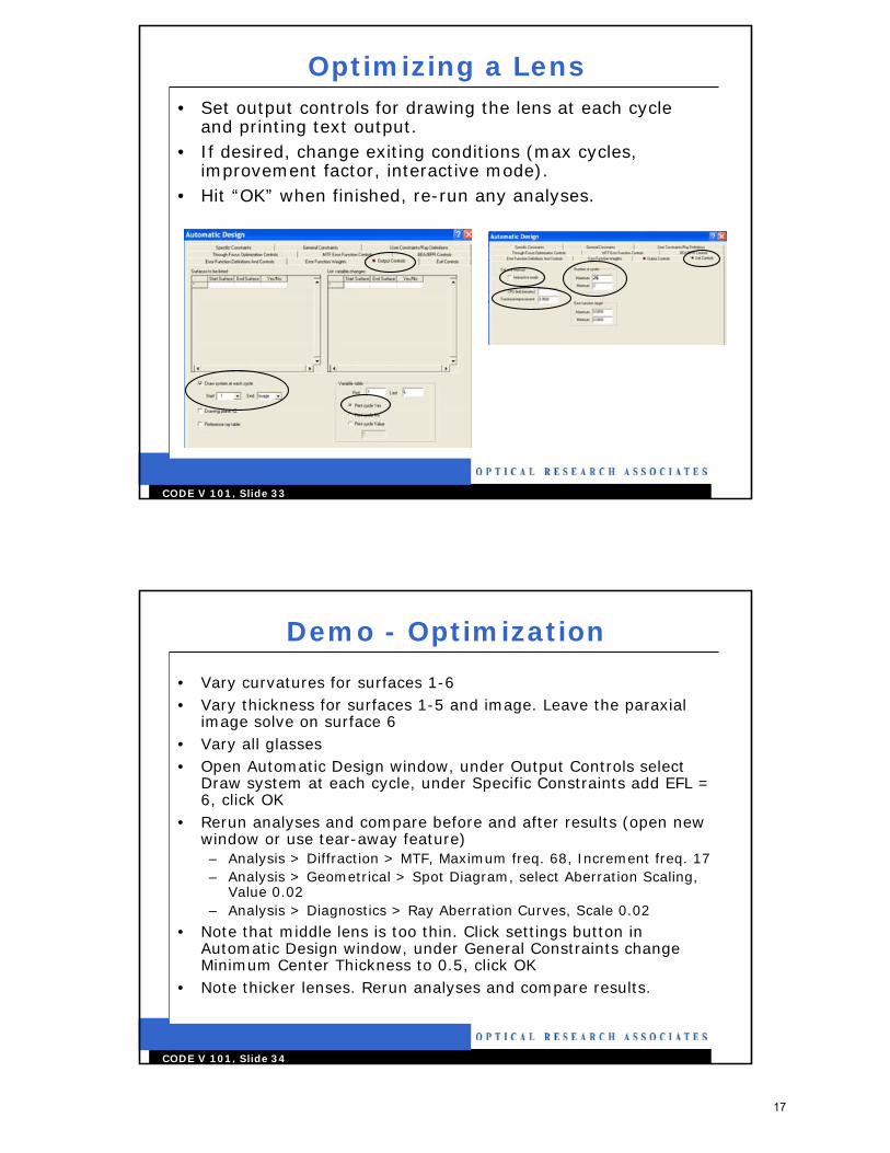
• Define any specific constraints (EFL, distortion, surface thicknesses, ray trace data, etc.). These may override general constraints.
• Note: exact constraints handled by linear algebra solutions (Lagrange multipliers) separate from error function, weighted constraints included in error function.
Exact constraintsWeighted constraintsUnused constraints
16
17
CODE V 101, Slide 33
Optimizing a Lens• Set output controls for drawing the lens at each cycle
and printing text output. • If desired, change exiting conditions (max cycles,
improvement factor, interactive mode). • Hit “OK” when finished, re-run any analyses.
CODE V 101, Slide 34
Demo - Optimization
• Vary curvatures for surfaces 1-6• Vary thickness for surfaces 1-5 and image. Leave the paraxial
image solve on surface 6• Vary all glasses• Open Automatic Design window, under Output Controls select
Draw system at each cycle, under Specific Constraints add EFL = 6, click OK
• Rerun analyses and compare before and after results (open new window or use tear-away feature)– Analysis > Diffraction > MTF, Maximum freq. 68, Increment freq. 17– Analysis > Geometrical > Spot Diagram, select Aberration Scaling,
Value 0.02– Analysis > Diagnostics > Ray Aberration Curves, Scale 0.02
• Note that middle lens is too thin. Click settings button in Automatic Design window, under General Constraints change Minimum Center Thickness to 0.5, click OK
• Note thicker lenses. Rerun analyses and compare results.
17
18
CODE V 101, Slide 35
Demo - Optimization
• Commandsin cv_macro:extlen 'or02248' ! load patent lens
fno 3.5 ! pupil spec for f/#
WTW W2 2 ! wavelength weight
yan 0 11 19 26.5 ! object field angles in Y
tit 'CODE V Demo' ! set title
vie;go ! 2D plot
in cv_macro:setvig ! set vignettingvie;go ! 2D layout
fir ! list 1st order data
SCA EFL S1..I-1 6 ! scale lens to EFL of 6
fir ! list 1st order data
mtf; mfr 68; ifr 17; go ! run MTF, max freq. 68, increment 17
spo; ssi .02; go ! run spot diagram, plot scale .02
rim; ssi .02; go ! run ray aberration curves, plot scale .02
ccy s1..6 0 ! vary curvatures
thc s1..5 0 ! vary thicknesses
thc si 0
gc1 s1 0 ! vary glasses
gc1 s3 0
gc1 s5 0
CODE V 101, Slide 36
Demo - Optimization
• Commands (cont’d)
aut;dra;efl=6;go ! optimize, draw the system at each cycle
mtf; mfr 68; ifr 17; go ! rerun analysis as before
spo; ssi .02; go
rim; ssi .02; go
aut;dra;efl=6;mnt .5;go ! optimize, set min thickness of .5
mtf; mfr 68; ifr 17; go ! rerun analysis as before
spo; ssi .02; go
rim; ssi .02; go
18
19
CODE V 101, Slide 37
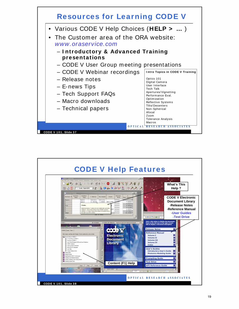
Resources for Learning CODE V
• Various CODE V Help Choices (HELP > … )• The Customer area of the ORA website:
www.oraservice.com– Introductory & Advanced Training
presentations– CODE V User Group meeting presentations– CODE V Webinar recordings– Release notes– E-news Tips– Tech Support FAQs– Macro downloads– Technical papers
Intro Topics in CODE V Training
Optics 101Digital CameraUser InterfaceTech TalkApertures/VignettingPerformance Eval.OptimizationReflective SystemsTilts/DecentersNon-SphericalAfocalZoomTolerance AnalysisMacros
CODE V 101, Slide 38
CODE V Help Features
What’s This Help ?
CODE V Electronic Document Library
-Release Notes-Reference Manual
-User Guides-Test Drive
Content (F1) Help
19
20
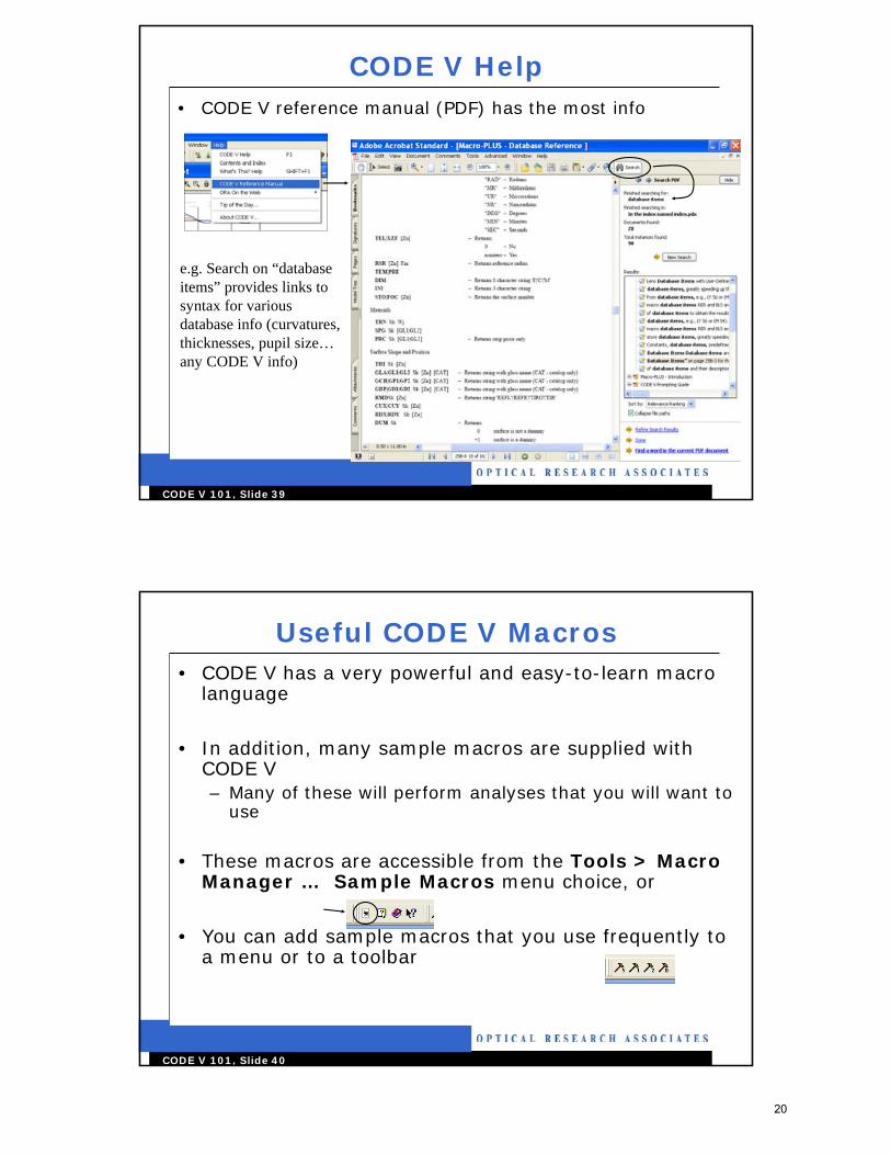
CODE V 101, Slide 39
CODE V Help• CODE V reference manual (PDF) has the most info
e.g. Search on “database items” provides links to syntax for various database info (curvatures, thicknesses, pupil size…any CODE V info)
CODE V 101, Slide 40
Useful CODE V Macros• CODE V has a very powerful and easy-to-learn macro
language
• In addition, many sample macros are supplied with CODE V– Many of these will perform analyses that you will want to
use
• These macros are accessible from the Tools > Macro Manager … Sample Macros menu choice, or
• You can add sample macros that you use frequently to a menu or to a toolbar
20
21
CODE V 101, Slide 41
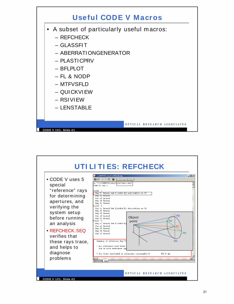
Useful CODE V Macros
• A subset of particularly useful macros:– REFCHECK– GLASSFIT– ABERRATIONGENERATOR– PLASTICPRV– BFLPLOT– FL & NODP– MTFVSFLD– QUICKVIEW– RSIVIEW– LENSTABLE
CODE V 101, Slide 42
UTILITIES: REFCHECK
•CODE V uses 5 special “reference” rays for determining apertures, and verifying the system setup before running an analysis
•REFCHECK.SEQverifies that these rays trace, and helps to diagnose problems
Objectpoint
R1
R3
R4
R5
R2
21
22
CODE V 101, Slide 43
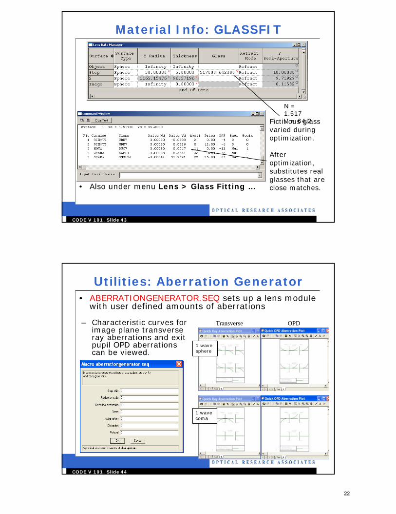
Material Info: GLASSFIT
• Also under menu Lens > Glass Fitting …
Fictitious glass varied during optimization.
After optimization, substitutes real glasses that are close matches.
N = 1.517V = 64.2
CODE V 101, Slide 44
Utilities: Aberration Generator• ABERRATIONGENERATOR.SEQ sets up a lens module
with user defined amounts of aberrations
1 wave sphere
1 wave coma
– Characteristic curves for image plane transverse ray aberrations and exit pupil OPD aberrations can be viewed.
Transverse OPD
22
23
CODE V 101, Slide 45
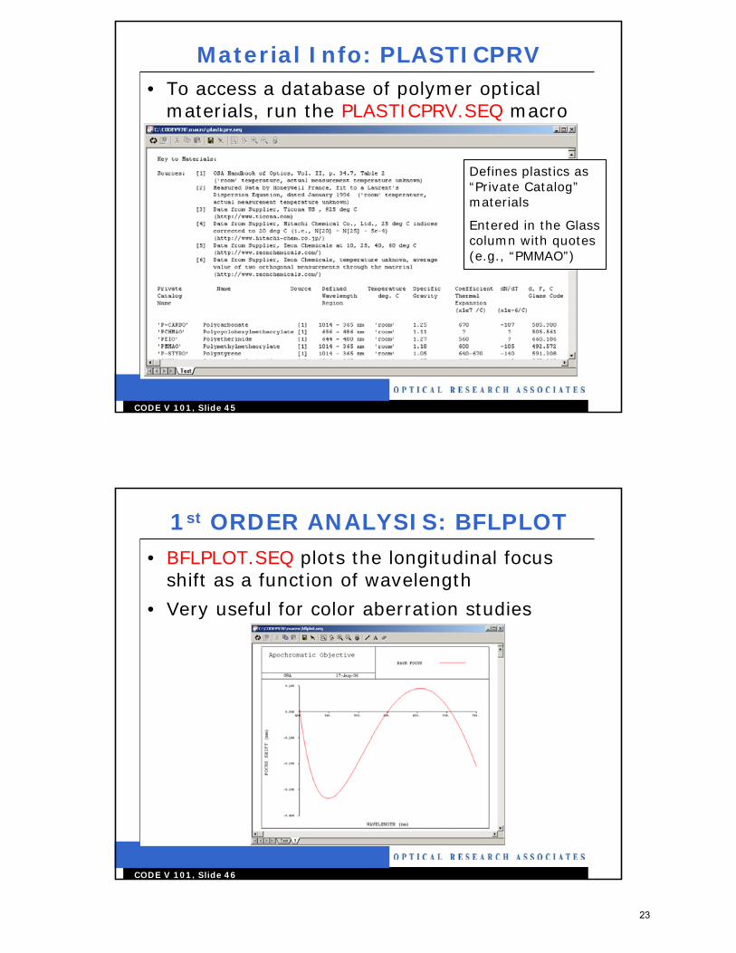
Material Info: PLASTICPRV• To access a database of polymer optical
materials, run the PLASTICPRV.SEQ macro
Defines plastics as “Private Catalog”materials
Entered in the Glass column with quotes (e.g., “PMMAO”)
CODE V 101, Slide 46
1st ORDER ANALYSIS: BFLPLOT• BFLPLOT.SEQ plots the longitudinal focus
shift as a function of wavelength
• Very useful for color aberration studies
23
24
CODE V 101, Slide 47
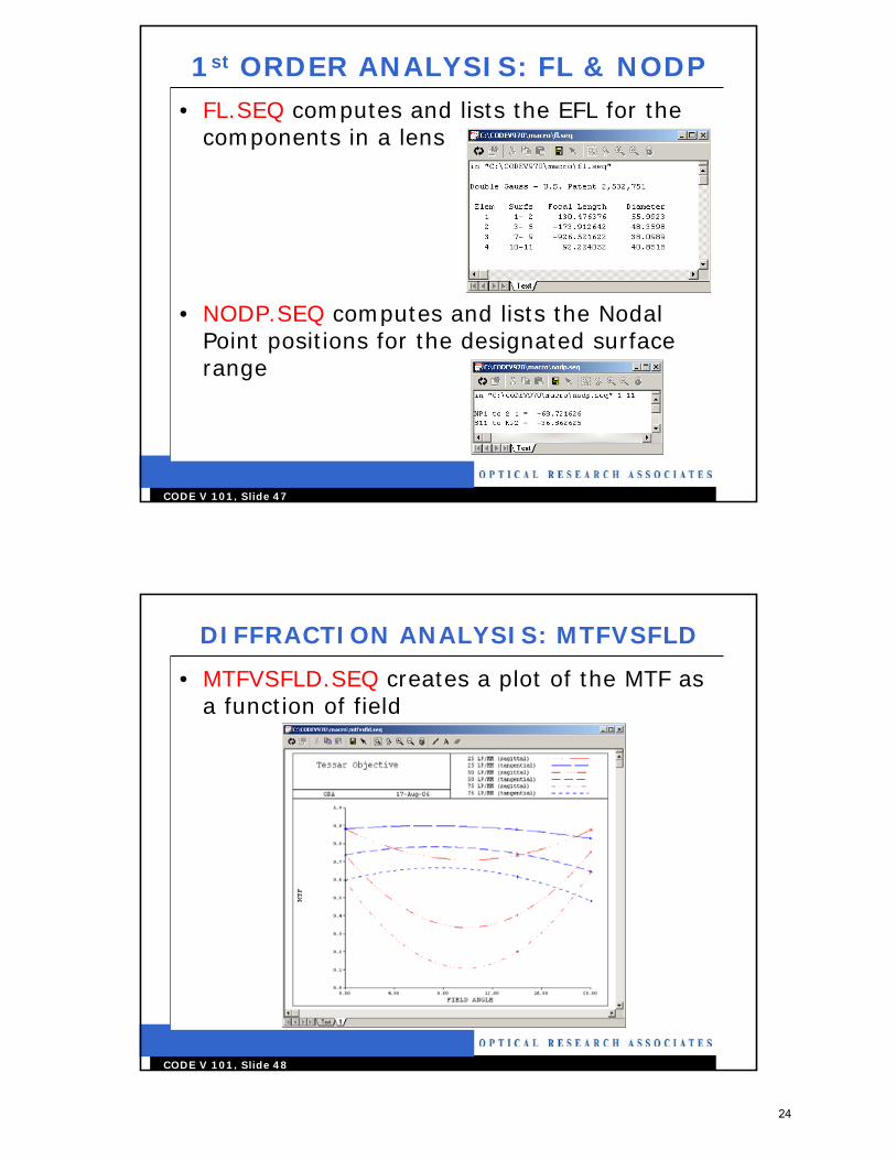
1st ORDER ANALYSIS: FL & NODP• FL.SEQ computes and lists the EFL for the
components in a lens
• NODP.SEQ computes and lists the Nodal Point positions for the designated surface range
CODE V 101, Slide 48
DIFFRACTION ANALYSIS: MTFVSFLD
• MTFVSFLD.SEQ creates a plot of the MTF as a function of field
24
25
CODE V 101, Slide 49
UTILITIES: QUICKVIEW
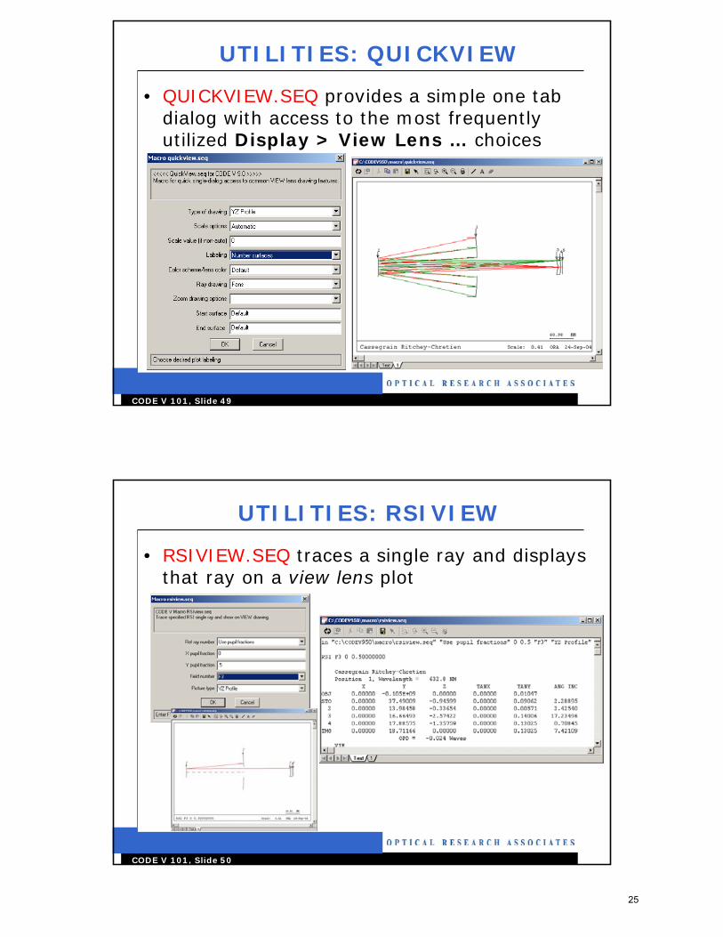
• QUICKVIEW.SEQ provides a simple one tab dialog with access to the most frequently utilized Display > View Lens … choices
CODE V 101, Slide 50
UTILITIES: RSIVIEW
• RSIVIEW.SEQ traces a single ray and displays that ray on a view lens plot
25
26
CODE V 101, Slide 51
FABRICATION SUPPORT: LENSTABLE
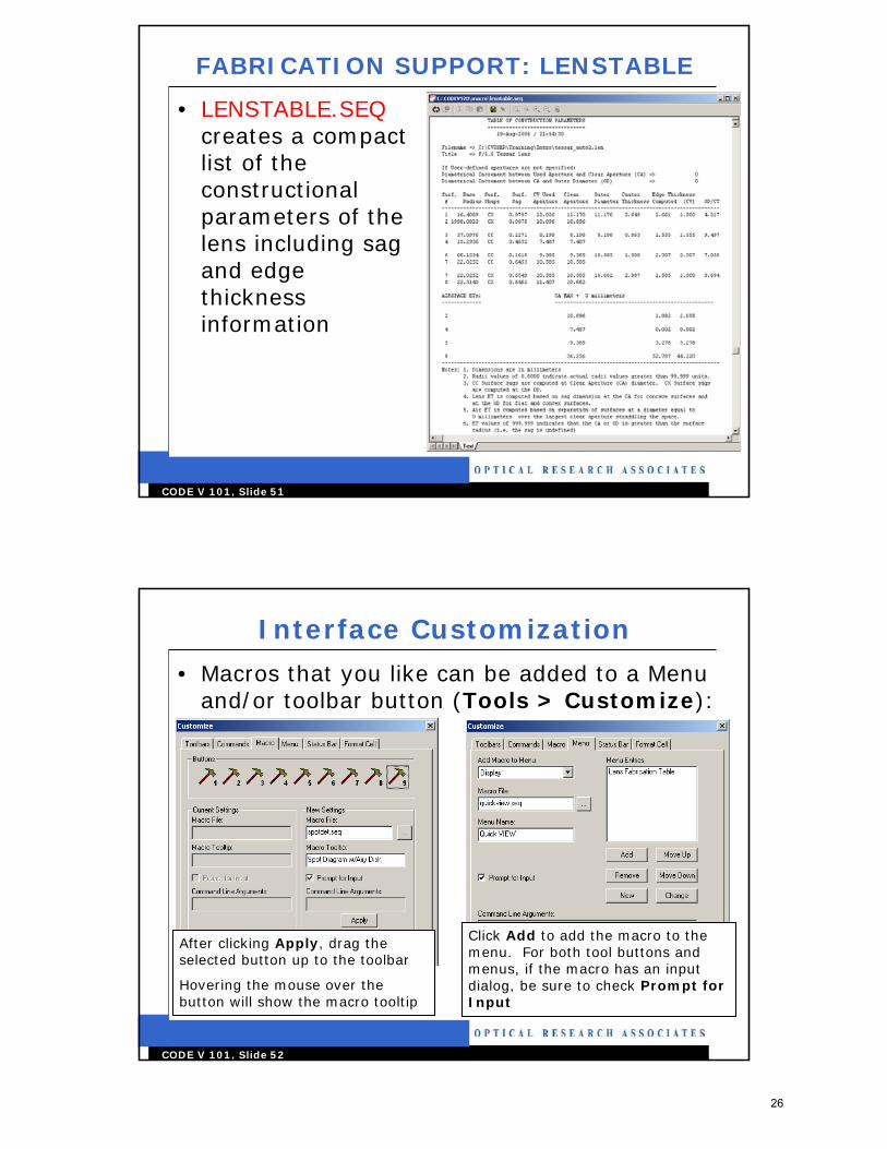
• LENSTABLE.SEQcreates a compact list of the constructional parameters of the lens including sag and edge thickness information
CODE V 101, Slide 52
Interface Customization
• Macros that you like can be added to a Menu and/or toolbar button (Tools > Customize):
After clicking Apply, drag the selected button up to the toolbar
Hovering the mouse over the button will show the macro tooltip
Click Add to add the macro to the menu. For both tool buttons and menus, if the macro has an input dialog, be sure to check Prompt for Input
26
27
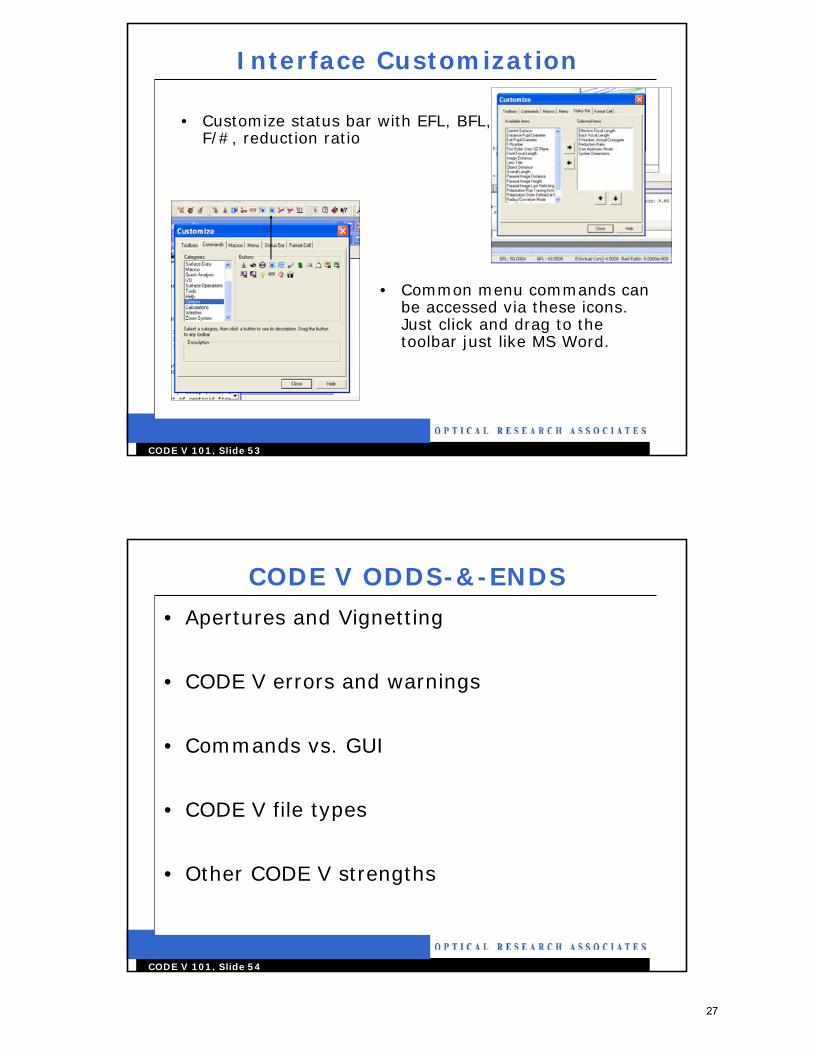
CODE V 101, Slide 53
Interface Customization
• Customize status bar with EFL, BFL, F/#, reduction ratio
• Common menu commands can be accessed via these icons. Just click and drag to the toolbar just like MS Word.
CODE V 101, Slide 54
CODE V ODDS-&-ENDS
• Apertures and Vignetting
• CODE V errors and warnings
• Commands vs. GUI
• CODE V file types
• Other CODE V strengths
27
28
CODE V 101, Slide 55
Odds & Ends: Apertures and Vignetting
• For accurate results in any optical design software, it is very important to understand how apertures are used– CODE V (and some other programs) also use
the concept of Vignetting factors, whose use should be understood
• Review the Apertures and Vignetting section from the Introduction to CODE V training– www.oraservice.com > Training Course Notes >
Introduction
CODE V 101, Slide 56
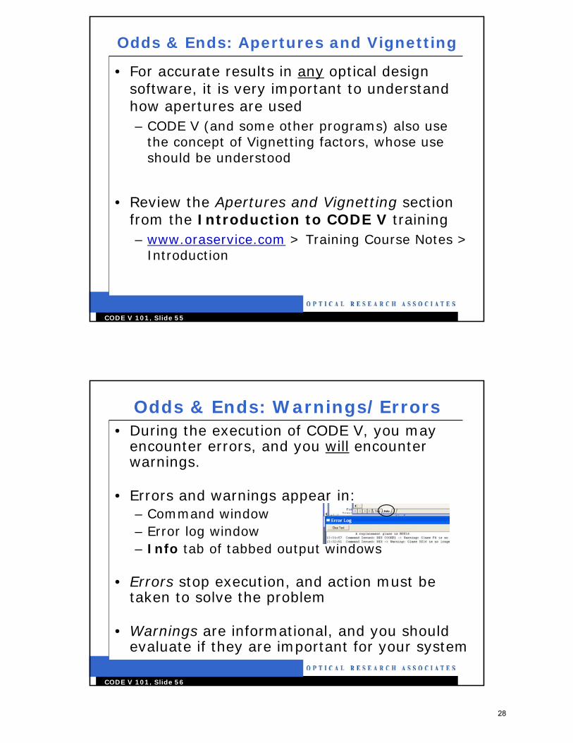
Odds & Ends: Warnings/Errors• During the execution of CODE V, you may
encounter errors, and you will encounter warnings.
• Errors and warnings appear in:– Command window– Error log window– Info tab of tabbed output windows
• Errors stop execution, and action must be taken to solve the problem
• Warnings are informational, and you should evaluate if they are important for your system
28
29
CODE V 101, Slide 57
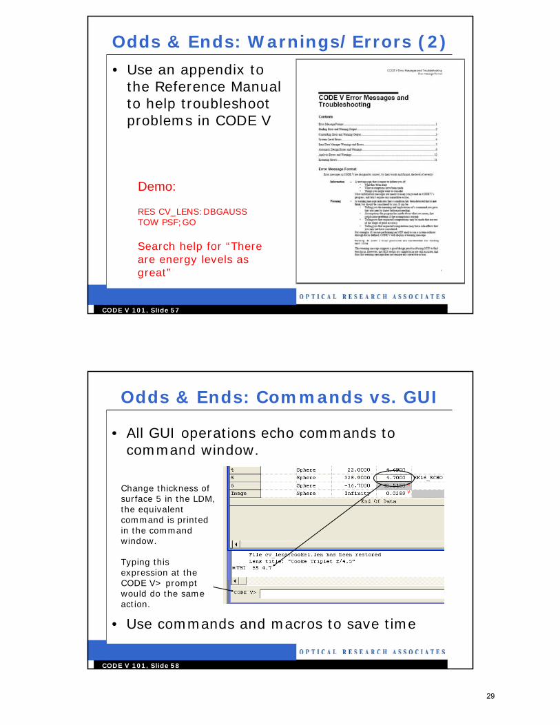
Odds & Ends: Warnings/Errors (2)
• Use an appendix to the Reference Manual to help troubleshoot problems in CODE V
Demo:
RES CV_LENS:DBGAUSSTOW PSF;GO
Search help for “There are energy levels as great”
CODE V 101, Slide 58
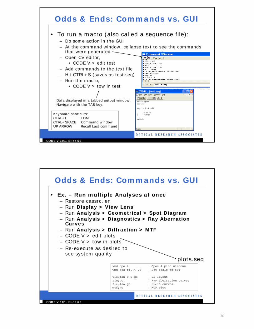
Odds & Ends: Commands vs. GUI
• All GUI operations echo commands to command window.
Change thickness of surface 5 in the LDM, the equivalent command is printed in the command window.
Typing this expression at the CODE V> prompt would do the same action.
• Use commands and macros to save time
29
30
CODE V 101, Slide 59
Odds & Ends: Commands vs. GUI
• To run a macro (also called a sequence file):– Do some action in the GUI– At the command window, collapse text to see the commands
that were generated– Open CV editor,
• CODE V > edit test– Add commands to the text file– Hit CTRL+S (saves as test.seq)– Run the macro,
• CODE V > tow in test
Data displayed in a tabbed output window. Navigate with the TAB key.
Keyboard shortcuts:CTRL+L LDMCTRL+SPACE Command windowUP ARROW Recall Last command
CODE V 101, Slide 60
Odds & Ends: Commands vs. GUI
• Ex. – Run multiple Analyses at once– Restore cassrc.len– Run Display > View Lens– Run Analysis > Geometrical > Spot Diagram– Run Analysis > Diagnostics > Ray Aberration
Curves– Run Analysis > Diffraction > MTF– CODE V > edit plots– CODE V > tow in plots
wnd ope 4 ! Open 4 plot windowswnd sca p1..4 .5 ! Set scale to 50%
vie;fan 0 5;go ! 2D layoutrim;go ! Ray aberration curvesfie;lsa;go ! Field curvesmtf;go ! MTF plot
plots.seq
– Re-execute as desired to see system quality
30
31
CODE V 101, Slide 61
Odds & Ends: Commands vs. GUI
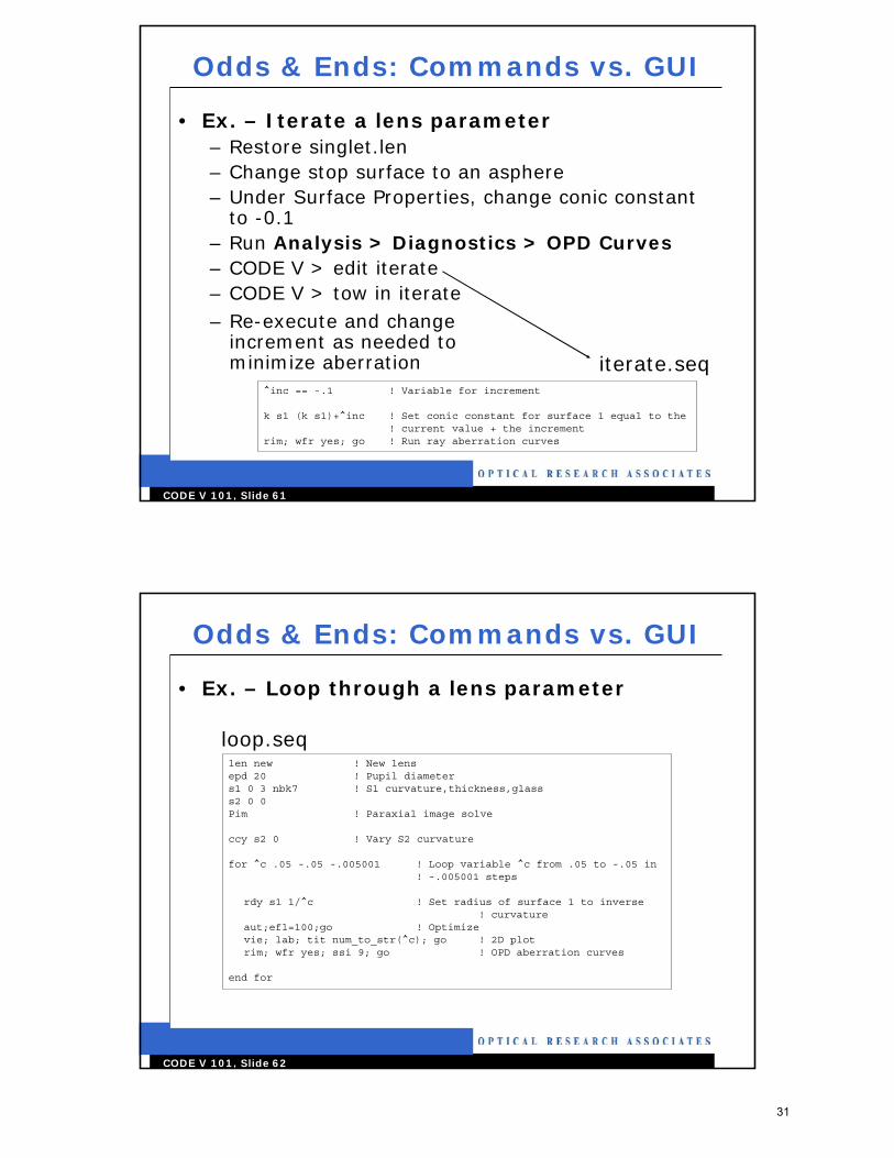
• Ex. – Iterate a lens parameter– Restore singlet.len– Change stop surface to an asphere– Under Surface Properties, change conic constant
to -0.1– Run Analysis > Diagnostics > OPD Curves– CODE V > edit iterate– CODE V > tow in iterate
^inc == -.1 ! Variable for increment
k s1 (k s1)+^inc ! Set conic constant for surface 1 equal to the ! current value + the increment
rim; wfr yes; go ! Run ray aberration curves
iterate.seq
– Re-execute and change increment as needed to minimize aberration
CODE V 101, Slide 62
Odds & Ends: Commands vs. GUI
• Ex. – Loop through a lens parameter
len new ! New lensepd 20 ! Pupil diameters1 0 3 nbk7 ! S1 curvature,thickness,glasss2 0 0Pim ! Paraxial image solve
ccy s2 0 ! Vary S2 curvature
for ^c .05 -.05 -.005001 ! Loop variable ^c from .05 to -.05 in! -.005001 steps
rdy s1 1/^c ! Set radius of surface 1 to inverse ! curvature
aut;efl=100;go ! Optimize vie; lab; tit num_to_str(^c); go ! 2D plotrim; wfr yes; ssi 9; go ! OPD aberration curves
end for
loop.seq
31
32
CODE V 101, Slide 63
Odds & Ends: Commands vs. GUI
• Ex. – Use database items to calculate desired data– CODE V > in calc_sf 1
^s == #1 ! Variable for surface #, uses input parameter
! Store db items for ROC values^r1 == (rdy s^s)^r2 == (rdy s^s+1)
^sf == (^r1 + ^r2)/(^r2 - ^r1) ! Eqn. for shape factor
wri 'Shape factor' ^sf ! Print results
calc_sf.seq
Shape factor
CODE V 101, Slide 64
Odds & Ends: Commands vs. GUI
• Ex. – Save data to buffer and plot results– Restore dbgauss.len
out n ! turn off output for faster execution ver n ! turn off echoing of commands
buf del b1 ! delete buffer 1 contents
^count == 0 ! variable to count # of points in loop
! loop variable ^w from 400 to 700, in steps of 10for ^w 400 700 10
^count == ^count + 1
wl ^w ! define a single wavelength for the system
buf del b0 ! delete the default buffer for recordingbuf y ! turn on recording of data into b0tra;go ! run transmission optionbuf n ! turn off recording of data into b0
bufplotTRA.seq
32
33
CODE V 101, Slide 65
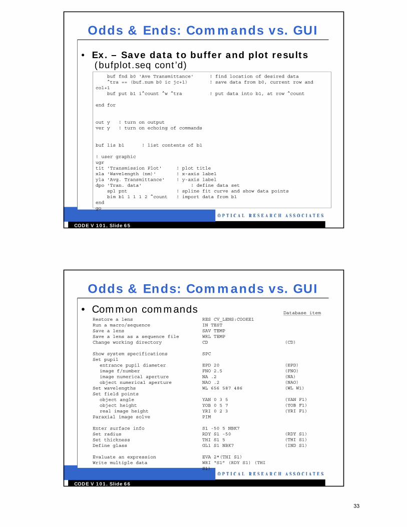
Odds & Ends: Commands vs. GUI
• Ex. – Save data to buffer and plot results
buf fnd b0 'Ave Transmittance' ! find location of desired data^tra == (buf.num b0 ic jc+1) ! save data from b0, current row and
col+1buf put b1 i^count ^w ^tra ! put data into b1, at row ^count
end for
out y ! turn on outputver y ! turn on echoing of commands
buf lis b1 ! list contents of b1
! user graphicugrtit 'Transmission Plot' ! plot titlexla 'Wavelength (nm)' ! x-axis labelyla 'Avg. Transmittance' ! y-axis labeldpo 'Tran. data' ! define data set
spl pnt ! spline fit curve and show data pointsbim b1 1 1 1 2 ^count ! import data from b1
end go
(bufplot.seq cont’d)
CODE V 101, Slide 66
Odds & Ends: Commands vs. GUI
• Common commandsRestore a lensRun a macro/sequenceSave a lensSave a lens as a sequence fileChange working directory
Show system specificationsSet pupil
entrance pupil diameterimage f/numberimage numerical apertureobject numerical aperture
Set wavelengthsSet field points
object angleobject heightreal image height
Paraxial image solve
Enter surface infoSet radiusSet thickness Define glass
Evaluate an expressionWrite multiple data
RES CV_LENS:COOKE1IN TESTSAV TEMPWRL TEMPCD
SPC
EPD 20FNO 2.5NA .2NAO .2WL 656 587 486
YAN 0 3 5YOB 0 5 7YRI 0 2 3PIM
S1 -50 5 NBK7RDY S1 -50THI S1 5GL1 S1 NBK7
EVA 2*(THI S1)WRI “S1” (RDY S1) (THI S1)
(CD)
(EPD)(FNO)(NA)(NAO)(WL W1)
(YAN F1)(YOB F1)(YRI F1)
(RDY S1)(THI S1)(IND S1)
Database item
33
34
CODE V 101, Slide 67
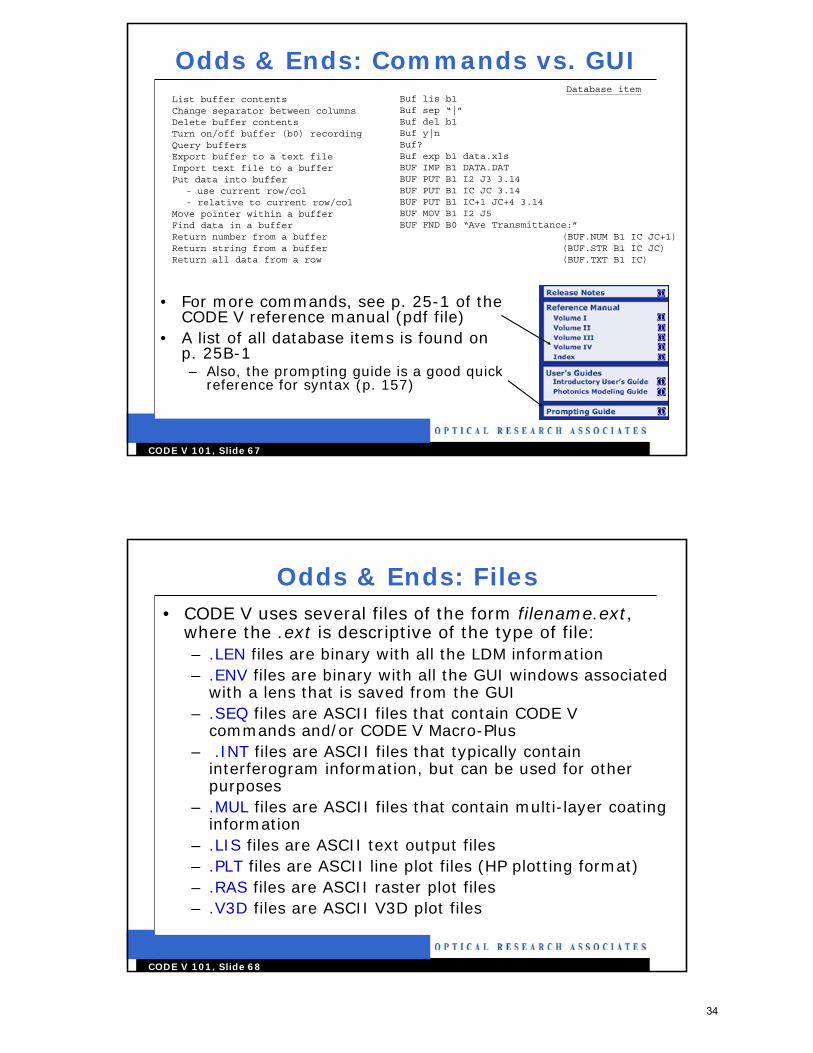
Odds & Ends: Commands vs. GUI
• For more commands, see p. 25-1 of the CODE V reference manual (pdf file)
• A list of all database items is found on p. 25B-1– Also, the prompting guide is a good quick
reference for syntax (p. 157)
List buffer contentsChange separator between columnsDelete buffer contentsTurn on/off buffer (b0) recordingQuery buffersExport buffer to a text fileImport text file to a bufferPut data into buffer
- use current row/col- relative to current row/col
Move pointer within a bufferFind data in a bufferReturn number from a bufferReturn string from a bufferReturn all data from a row
Buf lis b1Buf sep “|”Buf del b1Buf y|nBuf?Buf exp b1 data.xlsBUF IMP B1 DATA.DATBUF PUT B1 I2 J3 3.14BUF PUT B1 IC JC 3.14BUF PUT B1 IC+1 JC+4 3.14BUF MOV B1 I2 J5BUF FND B0 “Ave Transmittance:”
(BUF.NUM B1 IC JC+1)(BUF.STR B1 IC JC)(BUF.TXT B1 IC)
Database item
CODE V 101, Slide 68
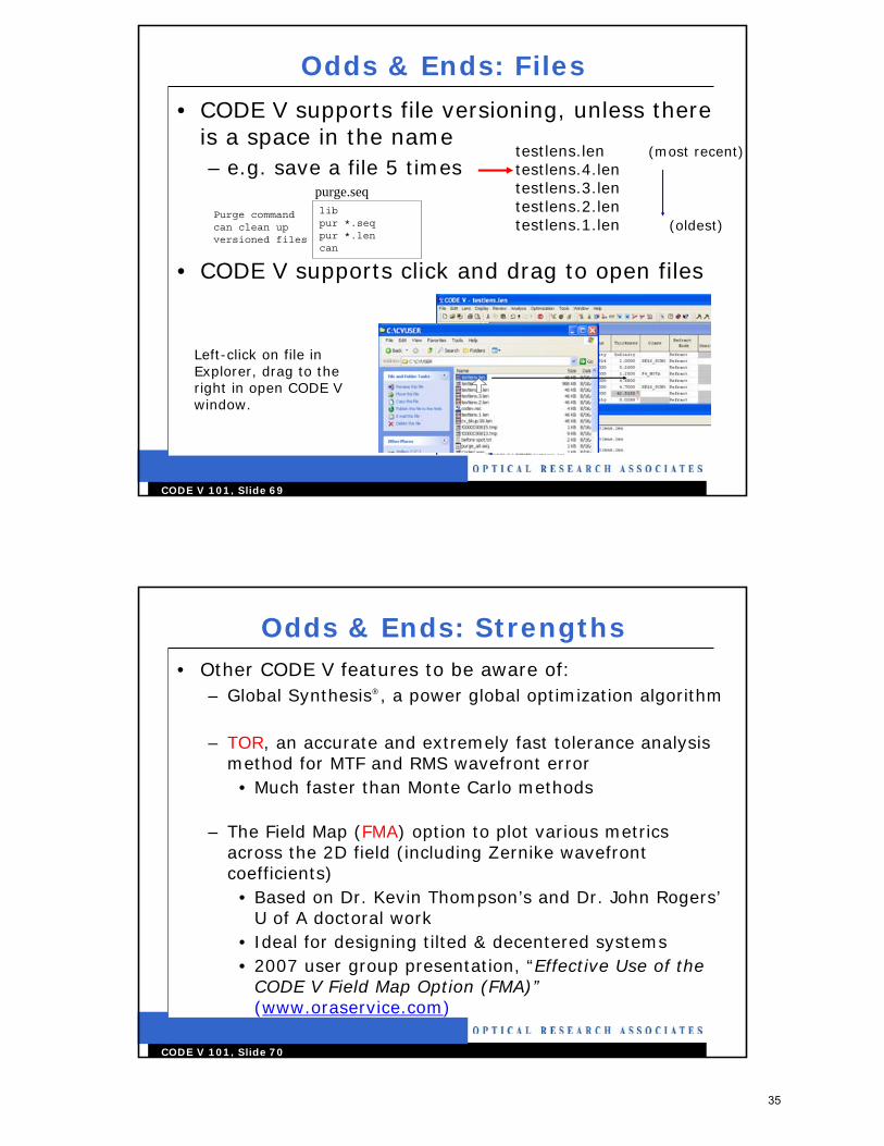
Odds & Ends: Files• CODE V uses several files of the form filename.ext,
where the .ext is descriptive of the type of file:– .LEN files are binary with all the LDM information– .ENV files are binary with all the GUI windows associated
with a lens that is saved from the GUI– .SEQ files are ASCII files that contain CODE V
commands and/or CODE V Macro-Plus– .INT files are ASCII files that typically contain
interferogram information, but can be used for other purposes
– .MUL files are ASCII files that contain multi-layer coating information
– .LIS files are ASCII text output files– .PLT files are ASCII line plot files (HP plotting format)– .RAS files are ASCII raster plot files– .V3D files are ASCII V3D plot files
34
35
CODE V 101, Slide 69
Odds & Ends: Files
• CODE V supports file versioning, unless there is a space in the name– e.g. save a file 5 times
• CODE V supports click and drag to open files
testlens.len (most recent)testlens.4.lentestlens.3.lentestlens.2.lentestlens.1.len (oldest)
Left-click on file in Explorer, drag to the right in open CODE V window.
lib pur *.seqpur *.lencan
purge.seq
Purge command can clean up versioned files
CODE V 101, Slide 70
Odds & Ends: Strengths• Other CODE V features to be aware of:
– Global Synthesis®, a power global optimization algorithm
– TOR, an accurate and extremely fast tolerance analysis method for MTF and RMS wavefront error• Much faster than Monte Carlo methods
– The Field Map (FMA) option to plot various metrics across the 2D field (including Zernike wavefront coefficients) • Based on Dr. Kevin Thompson’s and Dr. John Rogers’
U of A doctoral work• Ideal for designing tilted & decentered systems• 2007 user group presentation, “Effective Use of the
CODE V Field Map Option (FMA)”(www.oraservice.com)
35
36
CODE V 101, Slide 71
Scale: 4.80 14-Aug-07
5.21 MM
Lens module –severe vignetting
Odds & Ends: Strengths
• Other CODE V features to be aware of:– A COM API supporting CODE V interfaces with
Excel, MATLAB, and other applications– 2D Image Simulation (IMS), the ability to
simulate the appearance of an input .BMP object as imaged by the CODE V lens system
1.0
0.9
0.8
0.7
0.6
0.5
0.4
0.3
0.2
0.1
MODULATION
90 180 270 360 450 540 630 720 810 900
SPATIAL FREQUEN CY ( CYCL ES/M M)
D IFF RACTI ON MTF
19-Jan-07
DIFFRACTION LIMIT
AXIS
T
R1.0 FIELD ( )-24.23 O
WAVELENGTH WEIGHT 500.0 NM 1
DEF OCUS ING 0.00000
Diff. limit
TR IMS Simulation
CODE V 101, Slide 72
Odds & Ends: IMS Ex. (latcolor)
Image Simulation(IMS)
! Use aberration macro to setup lens module with 0.1 wvs sphericalin “c:\CODEV101\macro\aberrationgenerator.seq" 0 0 0.1 0 0 0 0
WL 656.3 587.6 486.1 ! add WL'sMCO S2 C7 3 ! 3 wvs W2 lateral colorMCO S2 C8 10 ! 10 wvs W3 lateral color
spo;go ! Spot diagramims;tgr 256; CME RGB; PDP YES; GO ! Image simulation
• Commands
SpotDiagram(SPO)
27-Aug-08
Thin Lens Module Aberration Generator
RAY ABERRATIONS ( MILLIMETERS )
656.3000 NM 587.6000 NM 486.1000 NM
-0.017944
0.017944
-0.017944
0.017944
0.00 RELATIVE
FIELD HEIGHT
( 0.000 )O
-0.017944
0.017944
-0.017944
0.017944
TANGENTIAL 1.00 RELATIVE SAGITTALFIELD HEIGHT
( 16.70 )O
Ray Aberration
Curves(RIM)
36
37
CODE V 101, Slide 73
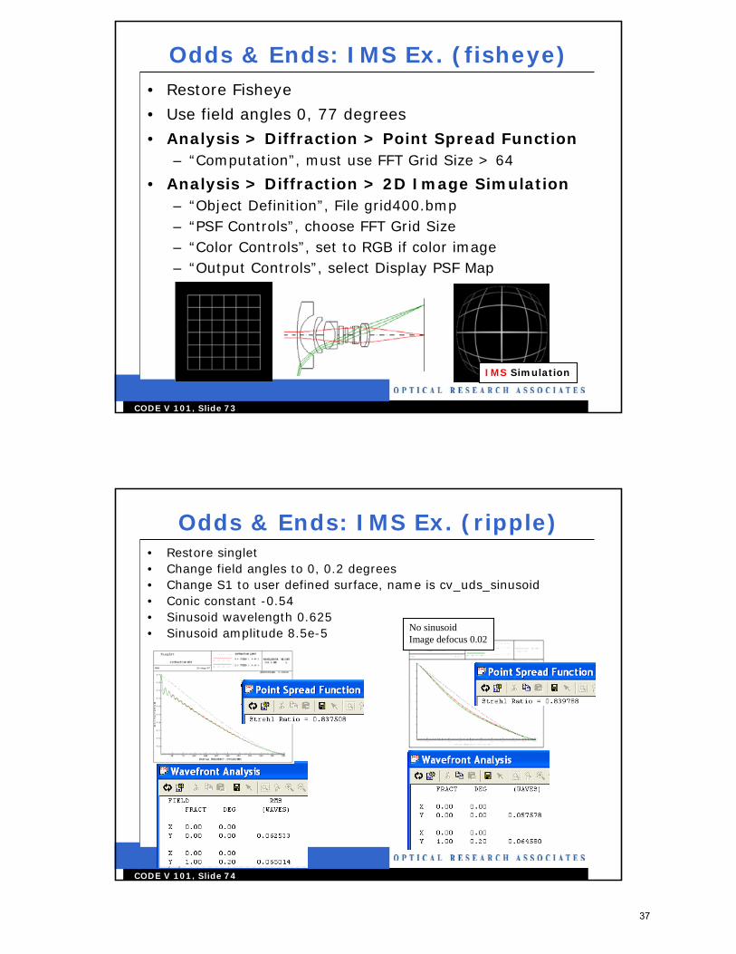
Odds & Ends: IMS Ex. (fisheye)• Restore Fisheye
• Use field angles 0, 77 degrees
• Analysis > Diffraction > Point Spread Function– “Computation”, must use FFT Grid Size > 64
• Analysis > Diffraction > 2D Image Simulation– “Object Definition”, File grid400.bmp– “PSF Controls”, choose FFT Grid Size– “Color Controls”, set to RGB if color image– “Output Controls”, select Display PSF Map
IMS Simulation
CODE V 101, Slide 74
Odds & Ends: IMS Ex. (ripple)• Restore singlet• Change field angles to 0, 0.2 degrees• Change S1 to user defined surface, name is cv_uds_sinusoid• Conic constant -0.54• Sinusoid wavelength 0.625• Sinusoid amplitude 8.5e-5 No sinusoid
Image defocus 0.02
37
38
CODE V 101, Slide 75
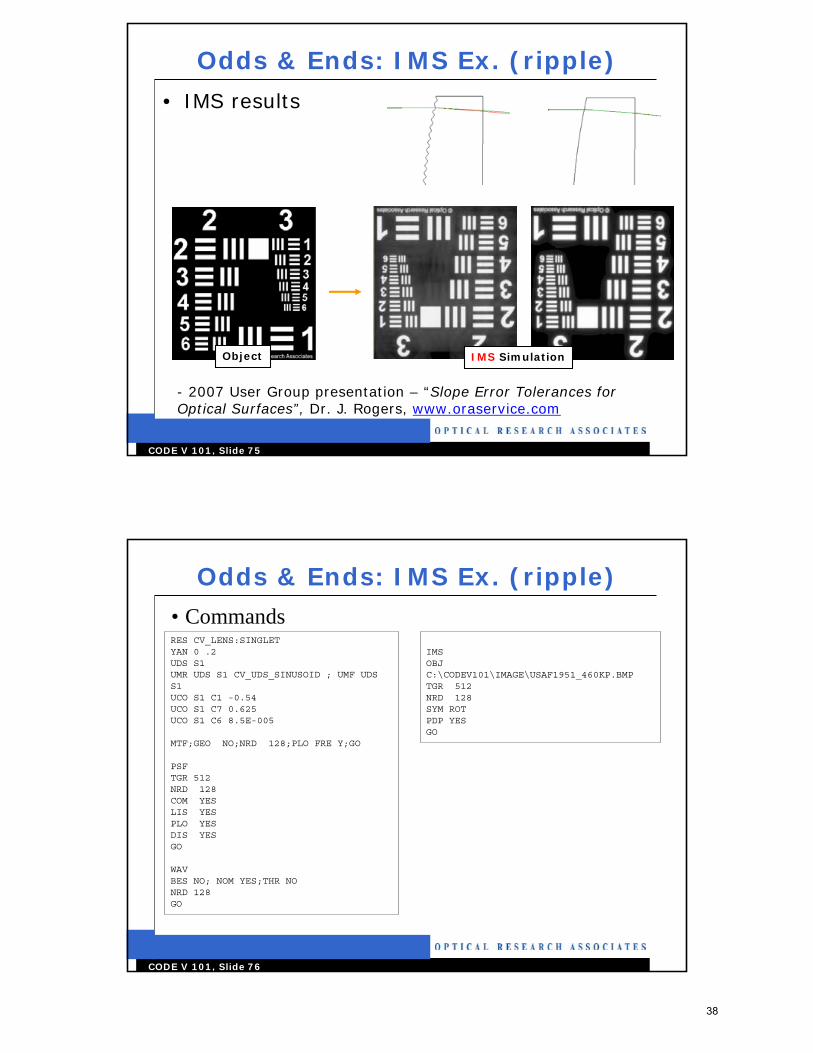
Odds & Ends: IMS Ex. (ripple)
• IMS results
IMS SimulationObject
- 2007 User Group presentation – “Slope Error Tolerances for Optical Surfaces”, Dr. J. Rogers, www.oraservice.com
CODE V 101, Slide 76
Odds & Ends: IMS Ex. (ripple)
RES CV_LENS:SINGLETYAN 0 .2UDS S1UMR UDS S1 CV_UDS_SINUSOID ; UMF UDS S1 UCO S1 C1 -0.54UCO S1 C7 0.625UCO S1 C6 8.5E-005
MTF;GEO NO;NRD 128;PLO FRE Y;GO
PSFTGR 512NRD 128COM YESLIS YESPLO YESDIS YESGO
WAVBES NO; NOM YES;THR NONRD 128GO
IMSOBJ C:\CODEV101\IMAGE\USAF1951_460KP.BMPTGR 512NRD 128SYM ROTPDP YESGO
• Commands
38
39
CODE V 101, Slide 77
Conclusions
• This covers a portion of the CODE V capabilities but should be enough for most of your classwork
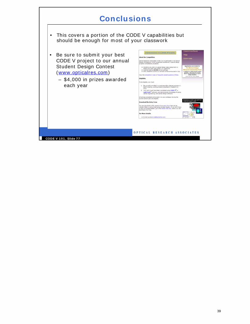
• Be sure to submit your best CODE V project to our annual Student Design Contest (www.opticalres.com)– $4,000 in prizes awarded
each year
39
Related Documents