Climate change and economic growth: An intertemporal ... · Climate change and economic growth: An intertemporal general equilibrium analysis for Egypt . Abeer Elshennawya, Sherman

1

Climate change and economic growth: An intertemporal general equilibrium analysis for Egypt

Abeer Elshennawya, Sherman Robinsonb, Dirk Willenbockelc,*

aAmerican University in Cairo, New Cairo 11835, P.O. Box 74, Egypt. [email protected] bInternational Food Policy Research Institute, 2033 K St NW, Washington, DC 20006-1002, USA. [email protected] cInstitute of Development Studies at the University of Sussex, Brighton BN1 9RE, UK. [email protected] *Corresponding author: Institute of Development Studies at the University of Sussex, Library Road, Brighton BN1 9RE, UK. Tel: +44 1273 915700.

Abstract: This study develops a multisectoral intertemporal general equilibrium model with forward-looking agents, population growth and technical progress to analyse the long-run growth prospects for Egypt in a changing climate. Based on a review of existing estimates of climate change impacts on agricultural productivity, labor productivity and the potential losses due to sea-level rise for the country, the model is used to simulate the effects of climate change on aggregate consumption, investment and welfare up to 2050. Available cost estimates for adaptation investments are employed to explore adaptation strategies. The simulation analysis suggests that in the absence of policy-led adaptation investments, real GDP towards the middle of the century will be nearly 10 percent lower than in a hypothetical baseline without climate change. A combination of adaptation measures, that include coastal protection investments for vulnerable sections along the low-lying Nile delta, support for changes in crop management practices and investments to raise irrigation efficiency, could reduce the GDP loss in 2050 to around 4 percent. JEL Codes: C68, D58, D90, E17, O44, Q54 Keywords: Climate change adaptation; Computable general equilibrium analysis; Scenario analysis; Dynamic CGE _______________ Paper for 17th Annual Conference on Global Economic Analysis, Dakar (Senegal), June 2014

2

1. Introduction

Due to the high concentration of economic activity along the low-lying coastal zone

of the Nile delta and its dependence on Nile river streamflow, Egypt's economy is

highly exposed to adverse climate change. Adaptation planning requires a forward-

looking assessment of climate change impacts on economic performance at economy-

wide and sectoral level and a cost-benefit assessment of conceivable adaptation

investments.

This study develops a multisectoral intertemporal general equilibrium model with

forward-looking agents, population growth and technical progress to analyse the long-

run growth prospects of Egypt in a changing climate. Based on a review of existing

estimates of climate change impacts on agricultural productivity, labor productivity

and the potential losses due to sea-level rise for the country, the model is used to

simulate the effects of climate change on aggregate consumption, investment and

welfare up to 2050. Available cost estimates for adaptation investments are employed

to explore adaptation strategies.

On the methodological side, the present study overcomes a basic limitation of existing

country-level recursive-dynamic computable general equilibrium models1

1 Examples for recent country-level studies using recursive-dynamic CGE models include Arndt et al (2011,2012), Robinson et al (2012) and Thurlow et al (2012). For an early study of this type for Egypt see Strzepek and Yates (2000). Fankhauser and Tol (2005) and Lecocq and Shalizi (2007) provide systematic conceptual discussions of the channels through which climate change potentially affects aggregate economic growth in Solow-type growth models, Cass-Koopmans-type optimal growth models and endogeneous growth models. Babiker et al (2009) compare recursive-dynamic and intertemporal specifications in global climate change mitigation modeling.

for climate

change impact analysis by incorporating forward-looking expectations. In contrast to

the standard recursive-dynamic approach, in which climate shocks hit agents in the

model by surprise, the intertemporal approach pursued here takes account of

endogenous anticipative adaptation responses to expected future climate change

impacts. Moreover, it extends the existing family of discrete-time intertemporal

computable general equilibrium models to which our model belongs by incorporating

population growth and technical progress. On the empirical side, the model is

calibrated to a social accounting matrix that reflects the observed current structure of

the Egyptian economy, and the climate change impact and adaptation scenarios are

informed by a close review of existing quantitative estimates for the size order of

impacts and the costs of adaptation measures.

3

The following section outlines the model and its numerical calibration. Section 3

specifies and motivates the climate change impact simulation scenarios. Section 4

presents simulation results in the absence of policy-led adaptation investments.

Section 5 considers adaptation scenarios, section 6 reflects briefly on sensitivity and

limitations of the analysis, and section 7 concludes.

2. The model

The determination of intertemporal saving and investment decisions in the model is

essentially a multi-sector open-economy extension of neoclassical optimal growth

theory in the Ramsey-Cass-Koopmans tradition, while intratemporal allocation

decisions across sectors are determined by a standard static small open economy CGE

model as described in full technical detail in Robinson et al (1999). The operational

model design draws upon the contributions to intertemporal CGE analysis and its

applications by Go (1994), Mercenier and Sampaio de Souza (1994), Diao and

Somwaru (1997), Elshennawy (2011) and Roe et al. (2010), but extends this class of

applied models by incorporating population growth and technical progress.

In line with its theoretical pedigree, the long-run steady-state growth rate of the model

is governed by labor force growth and the rate of technical progress, while climate

impacts that affect savings and investment entail level shifts in the time paths of GDP,

consumption and other macroeconomic aggregates without affecting the long-run

trend growth rate.

For purposes of the present study, the model distinguishes six sectors of economic

activity: agriculture, oil, industry, construction, electricity and services. Output is

produced using intermediate inputs and primary factors of production which include

labor and capital. To capture the impact of different policy scenarios on the labor

market, two skill categories of labor are distinguished, production and nonproduction

labor. For simplicity, the role of government is confined to tax collection. Tax

revenue is redistributed to the household sector and government expenditure is treated

as part of household consumption. The agents in the model are a representative

household with infinite planning horizon, a representative firm in each of the

production sectors, and the rest of the world, which is linked to the domestic economy

via trade, transfer and capital flows. Markets are perfectly competitive. What follows

is a description of the dynamic components of the model.

4

2.1. Consumption behavior

The representative household receives labor and dividend income from firms as well

as net transfer income from the rest of the world and the re-transfer of tax revenue.

The household chooses the path of consumption that maximizes the intertemporal

utility function

(1) 𝑈𝑜 = ∑ 𝑁𝑡 ln �𝐶𝑡𝑁𝑡� 1

(1+𝜌)𝑡 = 𝑁0 ∑ 𝑙𝑛 �𝐶𝑡𝑁𝑡� �1+𝑛

1+𝜌�𝑡

∞𝑡=0

∞𝑡=0

subject to the intertemporal budget constraint

(2) ∑ 𝑅𝑡𝑃𝑡𝐶𝑡 ≤ ∑ 𝑅𝑡[𝑤𝑝𝑡𝐿𝑃𝑡 + 𝑤𝑛𝑡𝐿𝑁𝑡 + 𝑇𝑅𝑡 + 𝑇𝑋𝑡] + 𝑊0∞𝑡=0

∞𝑡=0

and a no-Ponzi-game transversality condition, where C is an index of aggregate real

consumption, N = LP + NP is household size with LP and NP denoting production

and non-production labor respectively, n is the rate of population and labor force

growth, ρ is the pure rate of time preference, P is the implicit consumer price index

dual to C, wp and wn are the wage rates for production and non-production labor, TR

denotes net transfer income from the rest of the world, TX is tax revenue, W0 is initial

financial net wealth of the household sector, which is equal to the total market value

of the firms owned by the representative household minus the initial external debt

owed to the rest of the world, and

(3) 𝑅𝑡 = ∏ 1/(1 + 𝑟𝑠)𝑡𝑠=0

is the discount factor where r denotes the world interest rate.

The first-order conditions for the maximization of (1) subject to (2) and the

transversality condition, which ensures that the given initial debt does not exceed the

present value of future current account surpluses, take the form

(4) 𝑃𝑡+1𝐶𝑡+1𝑃𝑡𝐶𝑡

1+𝜌1+𝑛

= 1 + 𝑟𝑡.

2.2. Investment behavior

In each model sector s, firms are aggregated into one representative firm which

finances all of its investment through retained earnings and thus the number of equitiy

shares issued remains constant. Managers seek to maximize the value of the firm.

Assuming perfect capital markets, asset market equilibrium requires equal rates of

returns (adjusted for risk) on all assets. This implies that firm’s equity must earn an

5

expected rate of return equal to that of a safe asset like foreign bonds as reflected in

the condition

(5) s s

s s

DIV Vr = +V V∆

where DIV is dividends, V is the value of the firm, ∆Vs =Vs,t - Vs,t-1 is the expected

annual capital gain on firm equity and r is the interest rate on foreign bonds.

Solving the above difference equation (5) forward yields

(6) 𝑉𝑡 = ∑ 𝑅𝑡𝐷𝐼𝑉𝑡∞𝑣=𝑡 .

The market value of the firm equals the discounted stream of future dividends.

Dividends distributed to the household sector equal operating surplus minus

investment expenditure:

(7) 𝐷𝐼𝑉𝑆,𝑡 = 𝑃𝑉𝐴𝑆,𝑡𝑓�𝑏𝐿𝑃𝑆,𝑡, 𝑏𝐿𝑁𝑆,𝑡,𝐾𝑆,𝑡� − 𝑤𝑝𝑡𝐿𝑃𝑆,𝑡 − 𝑤𝑛𝑡𝐿𝑁𝑆,𝑡 − 𝑃𝐼𝑆,𝑡𝐼𝑡 − 𝐴𝐷𝐶𝑆,𝑡,

where, f (.) is the production function, K is capital, PI is the price per unit of

investment I, PVA is the value added price (output price net of indirect production

taxes and intermediate input unit costs) and ADC represents adjustment costs

associated with the installation of new capital:

(8) 𝐴𝐷𝐶𝑆,𝑡 = 𝑃𝐼𝐴𝑆,𝑡𝜑𝐼𝑆,𝑡2

𝐾𝑆,𝑡

Due to the presence of these adjustment costs, the capital stock does not adjust

instantaneously to its new optimal long-run level following exogenous shocks that

affect the return to capital. Adjustment costs to investment are assumed to be internal

to the firm. For any given level of the capital stock these costs are strictly increasing

in investment and decreasing in the capital stock for any given level of investment.

As a result, firms will find it optimal to increase the capital stock gradually over time

in order to reach the optimal long run capital intensity. The adjustment cost function

is assumed to be linear-homogeneous in investment and capital. Along with the

assumption of constant returns to scale in production, the linear homogeneity of the

adjustment cost function entails that Tobin’s marginal q equals Tobin’s average q

(Hayashi, 1982). In the general equilibrium model, the real adjustment costs take the

form of purchases of installation services, which are a Leontief composite of the

construction and industry commodities, and PIA is the unit price of this composite.

The model incorporates labor-augmenting technical progress. The labor efficiency

parameter b in (7) grows at the uniform exogenous rate g.

6

In each sector producers maximize the value of the firm subject to the capital

accumulation constraint

(9) 𝐾𝑆,𝑡+1 = (1 − 𝛿𝑆)𝐾𝑆,𝑡 + 𝐼𝑆,𝑡 ,

where δ is the rate of depreciation. Differentiating the Lagrangean for this

optimization with respect to the control variable I yields

(10) 𝑞𝑆,𝑡 = 𝑃𝐼𝑆,𝑡 + 2𝑃𝐼𝐴𝑆,𝑡𝜑𝐼𝑆,𝑡𝐾𝑆,𝑡

,

which determines the shadow price of capital. Condition (10) states that the firm

invests until the cost of acquiring capital – which is equal to the price of a unit of

investment plus marginal adjustment costs – is equal to the value of capital.

Differentiating with respect to the state variable K yields the no arbitrage condition

(11) 𝑃𝑉𝐴𝑆,𝑡𝑓𝐾 + 𝑃𝐼𝐴𝑆,𝑡𝜑 �𝐼𝑆,𝑡𝐾𝑆,𝑡

�2

+ (1 − 𝛿)𝑞𝑆,𝑡 − (1 + 𝑟)𝑞𝑆,𝑡−1 = 0 .

According to Equation (11), the value of the marginal product of capital PVA fK plus

the marginal reduction in adjustment costs brought by the increase in capital plus the

capital gains qt - q t-1 minus depreciation δq must equal the amount foregone rq by

choosing to accumulate this extra unit of capital. For simplicity, there is no

differentiation between government and private investment in the model. IS,t is a

Cobb-Douglas composite good over commodity groups demanded for investment

purposes,

(12) ,, ,

S SS t S S S SI AK INVD

θ // /= ∏ ,

where INVDS’,S is investment demand by sector S for goods of type S’ and AKS is a

constant parameter. PIS,t is the investment price index dual to IS,t .

2.3. Current account dynamics

The current account dynamics associated with the optimal consumption and

investment path is described by

(13) 𝐷𝑡+1 − 𝐷𝑡 = 𝑟𝑡𝐷𝑡 + 𝑇𝐵𝑡 + 𝑇𝑅𝑂𝑊𝑡 ,

where TBt is the trade balance surplus in t and TROW denotes exogenous net

transfers from abroad. Letting Y denote aggregate GDP, TBt = Yt - PtCt - ∑S PIS,tIS,t.

The no-Ponzi-game condition invoked in the derivation of the optimal consumption

path described by (4) entails that the initial debt inherited from the path constrains the

future path of domestic absorption, so that D0 = PV(Yt+TROWt) – PV(PtCt) – PV(∑S

PIS,tIS,t), where PV(x) denotes the present value of a stream xt discounted at rate r. In

7

other words, the initial debt must be matched by a corresponding positive present

value of future primary account surpluses.

2.4. Intratemporal general equilibrium

Embedded in this dynamic structure is a standard within-period general equilibrium

model that determines intratemporal relative prices, the sectoral allocation of labor

and the commodity composition of consumption, imports and exports.

Producers in the model are price takers in output and input markets and use constant

returns to scale technologies described by constant elasticity of substitution (CES)

value added functions and a Leontief fixed-coefficient technology for intermediate

input requirements by commodity group. The decision of producers between

production for domestic and foreign markets is governed by constant elasticity of

transformation (CET) functions that distinguish between exported and domestic goods

in each traded commodity group. Under the small-country assumption, Egypt faces

perfectly elastic world demand for its exports at fixed world prices. The profit-

maximizing equilibrium ratio of exports to domestic goods in any traded commodity

group is determined by the relative prices for these two commodity types.

On the demand side, imported and domestic goods are treated as imperfect substitutes

in both final and intermediate demand. In line with the small-country assumption,

Egypt faces an infinitely elastic world supply at fixed world prices. The equilibrium

ratio of imports to domestic goods is determined by the intratemporal felicity- and

cost-minimizing decisions of domestic agents based on the relative tax-inclusive

prices of imports and domestic goods.

2.5. Properties of the steady-state equilibrium growth path

Technically the dynamic system described by (1) to (13) can be reduced to a

saddlepoint-stable system in the state variable K and co-state variable q. K0 is

predetermined while q0 is a jump variable. In the absence of shocks to the exogenous

parameters of the model, the system can be shown to converge to a steady-state

equilibrium, in which q and the sectoral capital stocks per effective labor unit

(KS/(b(LN+LP)) are stationary, while aggregate income, consumption, investment and

other macro aggregates grow at the steady-state growth rate z = g + n + gn, provided

that (using asterisks to denote steady-state levels of variables) r* = ρ +g + ρg.

The steady-state investment ratio in each sector is

8

(14) 𝐼𝑆,𝑡∗

𝐾𝑆,𝑡∗ = 𝛿 + 𝑧 .

The net foreign asset position along the steady-growth path evolves according to

(15) (𝑟∗ − 𝑧)𝐷𝑡∗ = 𝑇𝐵𝑡∗ + 𝑇𝑅𝑂𝑊𝑡∗.

The steady-state growth path market value of the firm in each sector obeys

(16) (𝑟∗ − 𝑧)𝑉𝑆,𝑡∗ = 𝐷𝐼𝑉𝑡∗.

2.6. Data and calibration

The model is calibrated using the 2006/2007 Social Accounting Matrix (SAM) for

Egypt. Assuming that the initial data represents an economy evolving along a steady

state growth path, parameters are calibrated so that the model generates a path with a

starting point that replicates the observed benchmark data set in the absence of

anticipated future climate shocks. This dynamic baseline path serves as the

benchmark for comparison for the climate change scenarios considered in the

following sections.

Calibration of all parameters for the intratemporal part of the model follows the

standard methods used in comparative-static CGE models. The dynamic calibration

proceeds as follows. Based on the UN medium population growth projections for

Egypt from 2010 to 2050, the average annual labor force growth rate is set to n = 0.07

and the growth rate of labor-augmenting technical progress is set to g = 0.025, hence

the steady-state growth rate z = 0.0322. The rate of capital depreciation is set to δ =

0.04. Total dividend payments are calculated as the difference between the observed

value of capital income (gross operating surplus) and the observed value of total

investment in the SAM. In order for the model to replicate these observed

magnitudes, the pure rate of time preference is set to ρ = 0.16, and the adjustment cost

parameter is set to φ = 1. These settings jointly determine the initial real capital stock

by sector (KS), qS and PIS via the steady-state equilibrium conditions, and the

parameters AKS in (12) follow residually.

3. Simulation scenarios

Scenario S0 simulates the counterfactual steady-state equilibrium growth path in the

absence of any climate change impacts and serves as the baseline for comparison with

the climate change impact and adaptation scenarios.

9

Scenario S1 considers the economy-wide consequences of adverse climate change

impacts on agricultural productivity. According to the 2007 SAM, the agricultural

sector contributes 13.2 percent to Egypt’s GDP at factor cost while it currently

provides livelihoods for more than 30 percent of the population. Agricultural activity

is largely confined to a small strip along the banks of the Nile river basin and the

coastal zone of the Nile delta. More than 90 percent of Egypt’s crop production is

irrigated and the Nile supplies 95% of the country’s total water needs (Agrawala et al,

2004). Precipitation over Egypt itself is low and does not significantly contribute to

Nile streamflow, and hence future water supplies depend critically upon climate

change impacts on rainfall and evapotranspiration - and adaptation responses to it - in

the upstream East African Nile riparian regions. Since the completion of the Aswan

Dam in 1972 which helps to cope with periodic upstream droughts, Egypt has been

reasonably well adapted to current climate variability but remains vulnerable to multi-

year droughts (Agrawala et al, 2004; Robinson et al, 2008).

Simulations towards 2100 with a hydrology model by Strzepek et al (2001) across

different GCM scenarios suggest “modest” to “dramatic” reductions in Nile flow into

Egypt in eight of the nine climate scenarios under consideration and reductions

towards 2040 in all of the scenarios. A more recent hydrological study by Beyene et

al. (2010) likewise concludes that Egyptian agricultural water supplies could be

negatively impacted by climate change, especially in the second half of the 21st

century.

Met Office (2011) and EEAA(2010) review existing studies of climate change

impacts on crop yields for Egypt based on crop model simulations. For the country’s

main staple crops – maize, rice and wheat – these studies suggest yield reductions on

the order of -11 to -19 percent by 2050 and by -20 to -36 percent by 2100. Livestock

productivity is also expected to be adversely affected due to harmful heat stress and

yield reductions for fodder crops under climate change (Met Office, 2011).

On the basis of these projections, scenario S1 assumes a gradual anticipated linear

reduction in agricultural total factor productivity (TFP) over the period 2010 to 2100

by 0.25 percentage-points per year relative to the baseline, so that agricultural TFP is

10 percent below baseline in 2050 and 22.5 percent below baseline in 2100. The

selection of yield reductions at the lower end of the spectrum of existing crop model

projections makes allowance for a degree of autonomous adaptation responses by

Egyptian farmers. It is worth emphasizing that due to the assumption of exogenous

10

labour-augmenting progress in the agricultural sector as in other sectors, this scenario

does not assume that agricultural productivity declines over time - rather, at each

point in time from 2010 onwards, productivity is lower than in the baseline scenario,

but continues to rise over time due to the presence of labor-augmenting technical

progress.

Scenario S2 considers potential impacts of sea-level rise (SLR) on the growth

prospects for the Egyptian economy. As the coastal zone of the Nile delta coast hosts

a number of highly populated including Alexandria, Port Said, Rosetta, and Damietta,

which are import centers of economic activity (Agrawala et al, 2004), global impact

studies identify Egypt as one of the most vulnerable countries to SLR (Dasgupta et al,

2009, 2011, Met Office, 2011). Based on DIVA model simulations, Hinkel et al

(2012) estimate annual SLR damage costs for Egypt in the absence of protective

adaptation investments on the order of 0.06% of GDP in 2100 for a +64cm SLR

scenario, and on the order of 0.18% of GDP for a +126cm SLR scenario. In contrast,

Dagupta et al (2009) estimate a considerably higher SLR loss of 6.4% GDP for Egypt

under a +100cm SLR scenario. We simulate disruptions to economic activity due to

SLR in the absence of coastal protection investments as anticipated adverse shocks to

TFP across all sectors that rise linearly in strength from 0 before 2015 to -2 percent of

baseline productivity in 2100.

Scenario S3 simulates the impact of an anticipated increase in the frequency of

extreme coastal storm surges on top of the impacts due to mean sea level rise, as

contemplated by Dasgupta et al (2011) and envisaged in EEAA (2010a). A further

motivation for this scenario is provided by Hanson et al (2011) who identify

Alexandria - which generates a significant fraction of Egypt’s GDP -, as one of the 20

port cities globally with the highest levels of exposure to extreme storm surges. This

speculative scenario serves to illustrate the model responses to anticipated temporary

shocks. The scenario assumes that extreme storm surges that destroy productive

capital in all sectors occur every ten years from 2030 onwards through to 2100. The

shocks are implemented through temporary one-off increases in the rate of capital

depreciation by one percentage-point.

Scenario S4 considers impacts of thermal stresses on labor productivity in a changing

climate. This potential impact channel is generally neglected in economic climate

change impact assessments. Hsiang (2010) provides a strong argument in favor of the

inclusion this channel and points to evidence from meta-studies that suggest that

11

beyond a temperature threshold of 27o C labor productivity drops by around 2 percent

per 1oC increase in temperature. A recent econometric study by Zivin and Neidell

(2010) for the USA suggests impacts of high temperatures on effective labor supply

beyond a 27o C threshold of a similar magnitude. Given daytime temperatures in

Egypt beyond this threshold for around 6 months per year and GCM temperature

projections for the country on the order of 3 to 3.5°C compared to a 1960-90 baseline

(Met Office, 2011), this scenario assumes a gradual linear drop in labor productivity

relative to the baseline growth path from 2010 towards -1.3 percent in 2050 and to - 3

percent in 2100.

Scenario S5 simulates the joint impact of the climate shocks considered in isolation in

S1 to S4. Adaptation scenarios and their underlying assumptions are described in

section 5.

4. Climate change impact simulations

In the counterfactual no-climate-change baseline scenario, the economy grows

steadily at the long-run equilibrium growth rate of 3.22 percent. This entails that

aggregate income and real income double by 2030 relative to initial levels and are 3.8

times their initial levels by 2050. Per-capita income doubles by 2035 and is 2.9 times

its 2007 level by 2050. These figures need to be kept in mind to maintain a proper

perspective on the climate change impact results presented below.

Scenario S1 considers adverse climate impacts on agricultural productivity that

gradually increase in strength over time from 2010 onwards. The time path of these

future productivity shocks, as described in the previous section, is disclosed at the

start of the simulation horizon, and agents in the present perfect foresight setting

revise their intertemporal consumption and investment plans in response to the bad

news. The first column of Table 1 reports the resulting percentage deviations from the

baseline growth path for macroeconomic aggregates in 2030 and 2050.2

2 While the model is technically solved at annual resolution for 110 time steps up to the year 2117 and is assumed to evolve along the new steady-state growth path beyond that point ad infinitum, the presentation of result focuses on the period up to 2050.

The

anticipated future productivity shocks lower the present value of expected GDP and

require a corresponding reduction in the present value of domestic absorption – that is

the sum of domestic consumption and investment expenditure – to obey the

intertemporal external balance constraint. As households have a preference for a

12

smooth consumption expenditure growth path over time3

Associated with these macroeconomic adjustments to the yield shocks is an increase

in the country’s net foreign asset position over time. As domestic absorption drops

immediately while the negative income impacts materialize later, the current account

balance rises initially and the external debt level grows at a lower rate than along the

baseline steady-state growth path. As a result debt service payments in subsequent

periods are lower than in the baseline, thus allowing to maintain a smooth

consumption expenditure growth path as the climate change impact become more

pronounced. Essentially the same intertemporal macro adjustment patterns emerge for

scenarios S2 to S5.

, nominal consumption drops

by 0.14 percent immediately after the announcement of the shocks, but then continues

to grow smoothly at the unchanged steady-state growth rate z from this lower level.

However, since the price index of consumption P rises over time as a result of

increases in the supply prices for domestic agricultural goods (Table 1), aggregate real

consumption levels – and hence intratemporal utility – drop significantly relative to

the baseline with the passage as the adverse climate change impacts on agricultural

yields become more severe over the decades. By 2050, aggregate real consumption is

3.6 percent below its baseline equilibrium level for the same year.

Table 1: Climate Change Impacts on Macro Aggregates (Percentage deviations from baseline growth path)

S1 S2 S3 S4 S5 Real Consumption0 -0.09 -0.05 -0.07 -0.06 -0.20 Real Consumption2030 -0.63 -0.22 -0.42 -0.12 -1.17 Real Consumption2050 -1.33 -0.66 -1.21 -0.23 -2.95 Real Investment0 -0.28 -0.12 -0.17 -0.02 -0.47 Real Investment2030 -2.49 -2.48 -2.79 -0.47 -5.55 Real Investment2050 -5.02 -5.61 -6.78 -1.00 -11.96 Nominal Consumption -0.14 -0.08 -0.11 -0.06 -0.3 Consumer Price Index2050 1.21 0.59 1.12 0.16 2.53 Real Capital Stock2050 -3.32 -3.54 -6.44 -0.65 -9.93 Welfare U0 (ρ=0.16) -0.04 -0.01 -0.02 -0.01 -0.07 Welfare U0 (ρ=0.05) -0.12 -0.06 -0.09 -0.02 -0.24 Real GDP2050 -3.86 -3.40 -5.46 -0.82 -9.84

S1: Agricultural yield impacts. S2: SLR impacts. S3: SLR impacts as in S2 plus decadal coastal storm surge damages. S4: Thermal stress impacts on labor productivity S5: Joint S1 and S3 and S5 impacts.

3 Recall that since r = ρ+g+ρg, condition (4) entails smooth consumption expenditure growth at the rate g+n+gn.

13

Looking at the sectoral results for Egyptian agriculture under scenario S1, net imports

of agricultural commodities rise strongly under this scenario, with real AGR imports

in 2050 rising by 11 percent above base line level and Egypt’s real AGR exports

dropping 48 percent below baseline level towards the middle of the century.

Agricultural output in 2050 is 9.5 percent below base (but still more than three times

as large as in the initial 2007 equilibrium). Interestingly, the 2050 agricultural capital

stock is slightly larger than in the baseline (Table 2) despite a significant drop in

Egypt’s agricultural output (Table 3), as the producer price increase for domestic

AGR output is sufficiently strong to make additional net investment in the sector

profitable.4

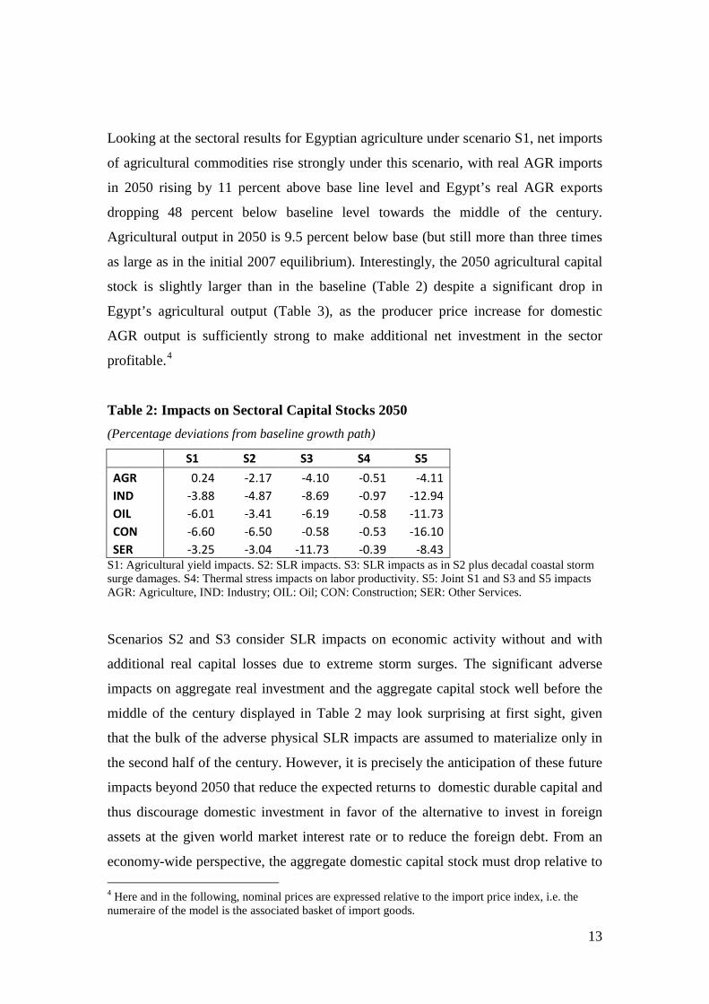
Table 2: Impacts on Sectoral Capital Stocks 2050 (Percentage deviations from baseline growth path)

S1 S2 S3 S4 S5 AGR 0.24 -2.17 -4.10 -0.51 -4.11 IND -3.88 -4.87 -8.69 -0.97 -12.94 OIL -6.01 -3.41 -6.19 -0.58 -11.73 CON -6.60 -6.50 -0.58 -0.53 -16.10 SER -3.25 -3.04 -11.73 -0.39 -8.43

S1: Agricultural yield impacts. S2: SLR impacts. S3: SLR impacts as in S2 plus decadal coastal storm surge damages. S4: Thermal stress impacts on labor productivity. S5: Joint S1 and S3 and S5 impacts AGR: Agriculture, IND: Industry; OIL: Oil; CON: Construction; SER: Other Services.

Scenarios S2 and S3 consider SLR impacts on economic activity without and with

additional real capital losses due to extreme storm surges. The significant adverse

impacts on aggregate real investment and the aggregate capital stock well before the

middle of the century displayed in Table 2 may look surprising at first sight, given

that the bulk of the adverse physical SLR impacts are assumed to materialize only in

the second half of the century. However, it is precisely the anticipation of these future

impacts beyond 2050 that reduce the expected returns to domestic durable capital and

thus discourage domestic investment in favor of the alternative to invest in foreign

assets at the given world market interest rate or to reduce the foreign debt. From an

economy-wide perspective, the aggregate domestic capital stock must drop relative to 4 Here and in the following, nominal prices are expressed relative to the import price index, i.e. the numeraire of the model is the associated basket of import goods.

14

the baseline growth path until the expected value of the marginal product of capital

has risen sufficiently to restore asset equilibrium. This anticipation effect is

completely absent in standard recursive-dynamic general equilibrium impact

assessment models, and the present illustrative simulations indicate that its impact on

economic growth can be quite significant.

Scenario S4 considers direct thermal stress impacts on labor productivity. As noted

earlier, this potential impact channel on economic performance has been commonly

neglected in previous economic climate change assessment studies. The simulation

results in Table 1 suggest a noticeable impact on aggregate economic outcomes.

Under the stated assumptions, real GDP in 2050 is projected to be 0.82 percent lower

than in the baseline and the aggregate capital stock drops by 0.65 percent below base,

which due to the impact of lower labor productivity on the expected returns to

domestic investment.

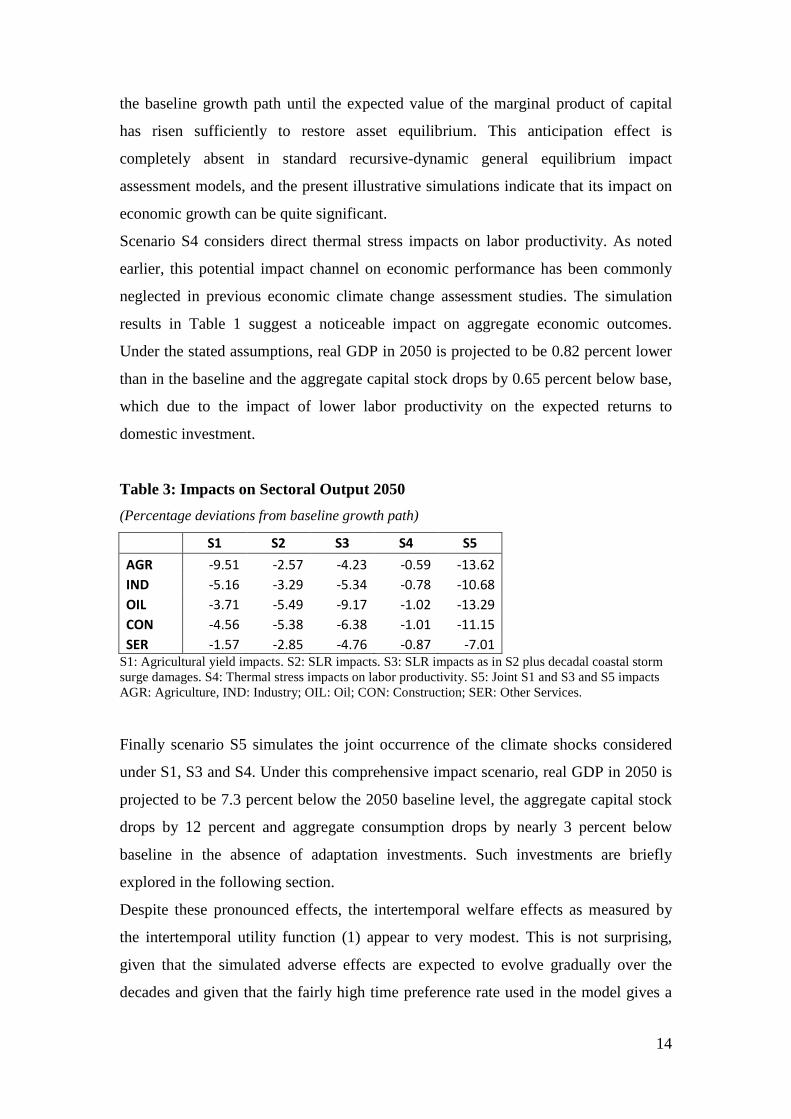
Table 3: Impacts on Sectoral Output 2050 (Percentage deviations from baseline growth path)

S1 S2 S3 S4 S5 AGR -9.51 -2.57 -4.23 -0.59 -13.62 IND -5.16 -3.29 -5.34 -0.78 -10.68 OIL -3.71 -5.49 -9.17 -1.02 -13.29 CON -4.56 -5.38 -6.38 -1.01 -11.15 SER -1.57 -2.85 -4.76 -0.87 -7.01

S1: Agricultural yield impacts. S2: SLR impacts. S3: SLR impacts as in S2 plus decadal coastal storm surge damages. S4: Thermal stress impacts on labor productivity. S5: Joint S1 and S3 and S5 impacts AGR: Agriculture, IND: Industry; OIL: Oil; CON: Construction; SER: Other Services.

Finally scenario S5 simulates the joint occurrence of the climate shocks considered

under S1, S3 and S4. Under this comprehensive impact scenario, real GDP in 2050 is

projected to be 7.3 percent below the 2050 baseline level, the aggregate capital stock

drops by 12 percent and aggregate consumption drops by nearly 3 percent below

baseline in the absence of adaptation investments. Such investments are briefly

explored in the following section.

Despite these pronounced effects, the intertemporal welfare effects as measured by

the intertemporal utility function (1) appear to very modest. This is not surprising,

given that the simulated adverse effects are expected to evolve gradually over the

decades and given that the fairly high time preference rate used in the model gives a

15

very low weight to consumption streams in a distant future (e.g. the weight attached to

aggregate real consumption in 2050 is 0.0017). If the same dynamic consumption

stream for S5 is evaluated with a lower time preference rate of ρ = 0.05, as is typically

employed in applied social cost-benefit analysis, the welfare loss rises by an order of

magnitude (Table 1), but still remains well below one percent.5

5. Stylized climate change adaptation scenarios

This section considers a range of adaptation investment options that aim to address

the climate change impacts analysed in section IV. EEAA (2010b) identifies a set of

priority actions for the agricultural sector including investments to improve surface

irrigation system efficiency and support for changes in crop and livestock

management practices. The study provides cost estimates for these measures over the

period 2010 to 2035, amounting to USD 3 billion, the bulk of which (USD 2.1 billion)

represents irrigation improvement measures. A casual glance at the relation of this

cumulated undiscounted cost figures to the cumulated economic losses under scenario

1 suggests that this adaptation option is potentially promising from a cost-benefit

perspective.

In simulation scenario S1A, we assume that the irrigation investments are entirely

domestically financed, while the research, extension, training and capacity building

services required to induce change in farming practices are provided in kind by

external experts and financed by international donors without notable additional

demands on domestic real resources. Following EEAA (2010b), it is assumed that the

capital investments are spread over the period 2010 to 2020, while maintenance and

repair costs arise in subsequent periods. The financing of the investment reduces the

investible funds available for other uses in the economy and the general equilibrium

model takes consistent account of this knock-on effect for other sectors. It is assumed

that the set of agricultural adaptation measures succeeds in reducing the adverse

productivity shocks simulated under scenario S1 by 50 percent at each point in time

from 2020 onwards, and thus this scenario allows for a considerable amount of

residual damage. A comparison of the aggregate results for S1A in Table 4 with the

5 Attaching low weights to the well-being of agents in the distant future is frequently criticized on intergenerational equity grounds, but if these agents are expected to enjoy a far higher per-capita income, this practice can likewise be justified on intergenerational equity grounds. For a detailed discussion within the context of an overlapping generations setting with finite life expectancies see Willenbockel (2008).

16

corresponding figures for S1 in Table 1 suggests a noticeable net beneficial impact of

the agricultural adaptation measures.

For protective coastal adaptation measures EEAA (2010b:24) estimates investment

costs on the order of USD 10,000 per meter of vulnerable coastline along the Nile

Delta, and deems 200km of coastline in need of protection, concluding (erroneously)

that “this would amount to about 2 million US$”. In scenario S3A we employ the

algebraically correct figure of USD 2 billion, which also appears to be more closely in

line with the annualized coastal adaptation cost estimates for Egypt reported in

Brown, S. et al (2010). This sizable figure amounts to circa 1.5 percent of Egypt’s

total GDP in 2007. Scenario S3A assumes that these investment costs are distributed

over a 10-year interval from 2020 to 2030 and adds annual maintenance and

replacement expenses equal to 5 percent of the initial investment expenditure

subsequently. We assume in this stylized scenario that under a medium-range SLR

scenario on the order of +50cm the protective measures are sufficient to avoid 80

percent of the economic losses simulated under the S3 scenario from 2030 onwards.

The comparison of results for S3A in Table 4 with results for S3 in Table 1 suggests

substantial net benefits for investments in coastal protection investments. The GDP

loss in 2050 is reduced by over 3.2 percentage-points in relation to the no-adaptation

scenario, and the drop in 2050 real consumption is reduced from -1.21 to -0.25

percent below the baseline level.

As an adaptation measure towards labor productivity losses from heat stresses, we

consider in scenario S4A the subsidised installation of additional cooling equipment

in industry and the services sector as a conceivable adaptation strategy. This raises the

demand for electricity and raises power prices for all sectors and households, and the

model takes account of this intersectoral spillover effect. It is assumed that the

annualized investment cost is on the order of 0.5 percent of the baseline investment

expenditure for the two sectors and that electricity demand in industry and services

rises by 2.5 percent per unit of output. We further assume that these investments

reduce the labor productivity losses imposed under S4 by 80 percent in industry and

by 60 percent in the service sector.

From an economy-wide perspective, the aggregate real consumption losses under S4A

remain very close to the losses under S4. This indicates that the gains due to higher

labor productivity associated with these adaptation measures are largely cancelled out

by the additional investment costs and the spillover effects of higher energy prices.

17

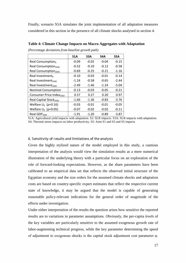
Finally, scenario S5A simulates the joint implementation of all adaptation measures

considered in this section in the presence of all climate shocks analysed in section 4.

Table 4: Climate Change Impacts on Macro Aggregates with Adaptation (Percentage deviations from baseline growth path)

S1A S3A S4A S5A Real Consumption0 -0.09 -0.02 -0.04 -0.15 Real Consumption2030 -0.52 -0.10 -0.12 -0.58 Real Consumption2050 -0.69 -0.25 -0.21 -1.16 Real Investment0 -0.10 -0.03 -0.01 -0.14 Real Investment2030 -1.24 -0.58 -0.65 -2.44 Real Investment2050 -2.49 -1.46 -1.24 -5.04 Nominal Consumption -0.13 -0.03 -0.05 -0.21 Consumer Price Index2050 0.57 0.27 0.20 0.97 Real Capital Stock2050 -1.66 -1.36 -0.83 -3.76 Welfare U0 (ρ=0.16) -0.03 -0.01 -0.01 -0.05 Welfare U0 (ρ=0.05) -0.07 -0.02 -0.02 -0.11 Real GDP2050 -1.91 -1.20 -0.89 -3.87

S1A: Agricultural yield impacts with adaptation. S2: SLR impacts. S3A: SLR impacts with adaptation. S4: Thermal stress impacts on labor productivity. S5: Joint S1 and S3 and S5 impacts

6. Sensitivity of r esults and limitations of the analysis

Given the highly stylized nature of the model employed in this study, a cautious

interpretation of the analysis would view the simulation results as a mere numerical

illustration of the underlying theory with a particular focus on an exploration of the

role of forward-looking expectations. However, as the share parameters have been

calibrated to an empirical data set that reflects the observed initial structure of the

Egyptian economy and the size orders for the assumed climate shocks and adaptation

costs are based on country-specific expert estimates that reflect the respective current

state of knowledge, it may be argued that the model is capable of generating

reasonable policy-relevant indications for the general order of magnitude of the

effects under investigation.

Under either interpretation of the results the question arises how sensitive the reported

results are to variations in parameter assumptions. Obviously, the per-capita levels of

the key variables are particularly sensitive to the assumed exogenous growth rate of

labor-augmenting technical progress, while the key parameter determining the speed

of adjustment to exogenous shocks is the capital stock adjustment cost parameter φ.

18

However, our prime interest is in the percentage deviations of variables from the

baseline growth path as a result of climate shocks, and both the signs and the broad

orders of magnitude of these percentage deviations are robust to variations in these

parameters. The direction of the reported intertemporal consumption smoothing

responses to anticipated shocks are likewise insensitive to behavioural parameter

constellations, given the assumption that the Egyptian economy can respond to shocks

to the returns to physical domestic capital via adjustments in the net foreign asset

position at a fixed world market interest rate.

This study analyzes only a limited set of stylized adaptation options, leaving plenty of

scope for more detailed future research to compare a wider set of carefully costed

adaptation measures. Other potentially fruitful avenues for further research are the

incorporation of uncertainty about climate shocks to relax the perfect foresight

assumption, the replacement of the counterfactual assumption of exponential

population growth at a constant rate by a logistic population growth specification

along the lines of Guerrini (2010), and extensions of the model to include endogenous

growth features.

7. Conclusions

This study develops a multisectoral intertemporal general equilibrium model with

forward-looking agents, population growth and technical progress to analyse the long-

run growth prospects of Egypt in a changing climate. Based on a review of existing

estimates of climate change impacts on agricultural productivity, labor productivity

and the potential losses due to sea-level rise for the country, the model is used to

simulate the effects of climate change on aggregate consumption, investment and

welfare up to 2050. Available cost estimates for adaptation investments are employed

to explore adaptation strategies.

The simulation analysis suggests that in the absence of policy-led adaptation

investments, real GDP towards the middle of the century will be nearly 10 percent

lower than in a hypothetical baseline without climate change. A combination of

adaptation measures, that include coastal protection investments for vulnerable

sections along the low-lying Nile delta, support for changes in crop management

practices and investments to raise irrigation efficiency, could reduce the GDP loss in

2050 to around 4 percent.

19

In contrast to existing recursive-dynamic computable general equilibrium models for

climate change impact assessment, the analysis takes expectation effects into account,

and this adds an important additional dimension to the assessment of households’ and

firms’ autonomous adaptation to climate change. Since current consumption and

investment decisions depend on expectations about the future, a dynamic climate

change impact analysis up to 2050 must take account of anticipations of future

climate change beyond 2050, and this is what the present study does.

In the small open-economy setting considered here, the anticipation of future adverse

climate change impacts beyond 2050 reduces the expected returns to domestic

durable capital and thus discourage domestic investment in favor of the alternative to

invest in foreign assets at the given world market interest rate or to reduce the foreign

debt. As a result, domestic capital accumulation slows down well before the severe

climate change impacts envisaged for the second half of the 21st century. This

anticipation effect is completely absent in standard recursive-dynamic general

equilibrium impact assessment models, and the simulations presented in this study

indicate that its impact on economic growth can be quite significant.

Acknowledgement Research for this study has been funded by Forum Euroméditerranéen des Instituts de Sciences Économiques – FEMISE.

20

References

Agrawala, S., Moehner, A., El Raey, M., Conway, D., van Aalst, M., Hagenstad, M., Smith, J., 2004. Development and Climate Change in Egypt: Focus on Coastal Resources and the Nile. OECD Environment Directorate, Paris. Arndt, C., Chinowsky, P., Strzepek, K., Thurlow, J., 2012. Climate change, growth and infrastructure investment: the case of Mozambique. Rev. Dev. Econ. 16, 463-475. Arndt, C., Robinson, S., Willenbockel, D., 2011. Ethiopia’s growth prospects in a changing climate: a stochastic general equilibrium approach. Global Environ. Chang. 21, 701-710. Babiker, M., Gurgel, A., Paltsev, S., Reilly, J. (2009) Forward-looking versus recursive-dynamic modelling in climate policy analysis. Econ. Model. 26, 1341-1354. Beyene, T., Lettenmaier, D.P., Kabat, P., 2010. Hydrologic impacts of climate change on the Nile river basin: implications of the 2007 IPCC scenarios. Climatic Change 100, 433-461. Brown, S., Kebede, A.S., Nicholls, R.J., 2010. Sea-Level Rise and Impacts in Africa, 2000 to 2100. University of Southampton, Southampton. Dasgupta, S., Laplante, B., Meisner, C., Wheeler, D., Yan, J., 2009. The impact of sea level rise on developing countries: a comparative analysis. Climatic Change 93, 379-388. Dasgupta, S., Laplante, B., Murray, S., Wheeler, D., 2011. Exposure of developing countries to sea-level rise and storm surges. Climatic Change 106, 567-579. Diao, X., Somwaru, A., 1997. Trade Creation and Trade Diversion under MERCORSUR: A Global Intertemporal General Equilibrium Analysis. University of Minnesota Department of Applied Economics Staff Paper P97-4. EEAA, 2010a. Egypt Second National Communication under the United Nations Framework Convention on Climate Change. Egyptian Environmental Affairs Agency, Cairo. EEAA, 2010b. Egypt National Environmental, Economic and Development Study (NEEDS) for Climate Change. Egyptian Environmental Affairs Agency, Cairo. Elshennawy, A., 2011. The Transitional Costs to Trade Liberalization: An Intertemporal General Equilibrium Model for Egypt. Society of Policy Modeling, EconModels.com. Fankhauser, S., Tol, R.S.J., 2005. On climate change and economic growth. Resour. Energy Econ. 27, 1-17. Go, D.,1994. External shocks, adjustment policies, and investment in a developing economy: illustrations from a forward-looking CGE model of the Philippines. J. Dev. Econ. 44, 229-261.

21

Guerrini, L., 2010. A closed-form solution to the Ramsey model with logistic population growth. Econ. Model. 27, 1178-1182. Hanson, S., Nicholls, R., Ranger, N., Hallegatte, S., Corfee-Morlot, J., Herweijer, C., Chateau, J., 2011. A global ranking of port cities with high exposure to climate extremes. Climatic Change 104, 89-111. Hayashi, F., 1982. Tobin’s marginal q and average q: a neoclassical interpretation. Econometrica 50, 675-693. Hinkel, J., Brown, S., Exner, L., Nicholls, R.J., Vafeidis, A.T., Kebede, A.S., 2012. Sea-level rise impacts on Africa and the effects of mitigation and adaptation: an application of DIVA. Reg. Environ. Change 12, 207–224. Hsiang, S.M., 2010. Temperatures and cyclones strongly associated with economic production in the Caribbean and Central America. P. Natl. Acad. Sci. USA 107, 15367-15372. Lecocq, F. and Shalizi, Z., 2007. How Might Climate Change Affect Economic Growth in Developing Countries? A Review of the Growth Literature with a Climate Lens. World Bank Policy Research Working Paper No. 4315. Mercenier, J., Sampaio de Souza, M.d.C., 1993. Structural adjustment and growth in a highly indebted market economy: Brazil, in: J. Mercenier, J., Srinivasan, T.N. (Eds.), Applied General Equilibrium Analysis and Economic Development: Present Achievements and Future Trends. University of Michigan Press, Ann Arbor, pp. 281-315. Met Office, 2011. Climate: Observations, Projections and Impacts. Egypt. Met Office, Exeter. Robinson, S., Willenbockel, D., Strzepek, K., 2012. A dynamic general equilibrium analysis of adaptation to climate change in Ethiopia. Rev. Dev. Econ. 16, 489-502. Robinson, S., Strzepek, K., El-Said, M., Lofgren, H., 2008. The high dam at Aswan, in: Bhatia, R., Cestti, R., Scatasta, M., Malik, R.P.S. (Eds.), Indirect Impact of Dams: Case Studies from India, Egypt and Brazil. World Bank and Academic Foundation, Washington, DC, and New Delhi, pp. 227-273. Robinson, S., Yunez-Naude, A., Hinojosa-Ojeda, R., Lewis, J.D., Devarajan, S., 1999. From stylized to applied models: building multisectoral CGE models for policy analysis. N. Am. J. Econ. Financ. 10, 5–38. Roe, T.L., Smith, R.B.W., Sirin Saracoglu, D., 2010. Multisector Growth Models: Theory and Application. Springer, New York. Strzepek, K., Yates, D., Yohe, G. Tol, R., Mader, N., 2001. Constructing ‘not implausible’ climate and economic scenarios for Egypt. Integr. Assessment 2, 139-157.

22

Strzepek, K.M., Yates, D.N., 2000. Responses and thresholds of the Egyptian economy to climate change impacts on the water resources of the Nile river. Climatic Change 46, 339-356. Thurlow, J., Dorosh, P., Yu, W., 2012. A stochastic simulation approach to estimating the economic impacts of climate change in Bangladesh. Rev. Dev. Econ. 16, 412-428. Willenbockel, D., 2008. Social time preference revisited. J. Popul. Econ. 21, 609-622. Zivin, J., Neidell, M., 2010. Temperature and the Allocation of Time: Implications for Climate Change. NBER Working Paper No. 15717.