Clearing, Counterparty Risk and Aggregate Risk · Clearing, Counterparty Risk and Aggregate Risk ... counterparty risk and aggregate risk ... with aggregate risk nests the model without

Clearing, Counterparty Risk and Aggregate Risk

Bruno Biais

Toulouse School of Economics

Florian Heider

European Central Bank

Marie Hoerova

European Central Bank

Paper presented at the 12th Jacques Polak Annual Research Conference

Hosted by the International Monetary Fund

Washington, DC─November 10–11, 2011

The views expressed in this paper are those of the author(s) only, and the presence

of them, or of links to them, on the IMF website does not imply that the IMF, its

Executive Board, or its management endorses or shares the views expressed in the

paper.

1122TTHH JJAACCQQUUEESS PPOOLLAAKK AANNNNUUAALL RREESSEEAARRCCHH CCOONNFFEERREENNCCEE NNOOVVEEMMBBEERR 1100––1111,, 22001111

Clearing, counterparty risk and aggregate risk∗

Bruno Biais† Florian Heider‡ Marie Hoerova§

October 2011

Abstract

We study the optimal design of clearing systems, focusing on counterparty riskinsurance and prevention. We study whether decentralized clearing improves on noclearing, and whether centralized clearing generates further improvement. We analyzehow counterparty risk should be allocated, whether traders should be fully insuredagainst that risk, and how moral-hazard affects the optimal allocation of risk. Themain advantage of centralized clearing is the mutualization of counterparty risk. Weshow, however, that the improved risk-sharing brought about by centralized clearingcan induce greater risk-taking, even in the first-best. Furthermore, while mutualizationis useful to share idiosyncratic risk, it cannot provide insurance against aggregate risk.When the latter is significant, it is necessary that protection buyers exert effort tofind robust counterparties. With moral hazard, this requires that they retain someexposure to counterparty risk.

JEL classification: G22, G24, G28, D82

Keywords: Risk-sharing; Moral hazard; Optimal contracting; Counterparty risk;Central Clearing Counterparty

∗We would like to thank Pierre-Olivier Gourinchas, Ayhan Kose, and Stijn Claessens for helpful commentson earlier drafts. The views expressed do not necessarily reflect those of the European Central Bank or theEurosystem. Biais gratefully aknowledges the support of the “Financial markets and investment bankingvalue chain”, sponsored by the Fédération des Banques Francaises.†Toulouse School of Economics, email: [email protected]‡European Central Bank, Financial Research Division, email: [email protected]§European Central Bank, Financial Research Division, email: [email protected]

1 Introduction

Counterparty risk is the risk to each party of a contract that his or her counterparty will

not live up to its contractual obligations. As vividly illustrated by the failure of Lehman

Brothers and the near failures of AIG and Bear Stearns, counterparty risk is a real issue

for investors. These episodes also suggest that some institutions should have paid more

attention to the risk that counterparties such as AIG or Lehman Brothers could default.

This, in turn, underscores that institutions should monitor the risk of their counterparties,

and ensure that they contract with creditworthy counterparties.

Clearing entities, and in particular Centralized Clearing Platforms (hereafter CCPs) can

offer insurance against counterparty risk. The clearing entity interposes between the two

parties. If one of them were unable to meet its obligations to the other, the clearing entity

would make the payment on behalf of the defaulting party. Would the development of CCPs

improve the working of markets? In September 2009, the G20 leaders, followed by the Dodd-

Frank Wall Street Reform & Consumer Protection Act, and then the European Commission,

answered yes. They proposed that all standardized OTC derivatives contracts be centrally

cleared.1

Was this the right move? More generally, how, and to what extent, can clearing improve

the allocation of risk and how should it be designed? Should it be decentralized or central-

ized? Should it provide full insurance against counterparty default? Is it likely to decrease

or increase risk-taking? Is clearing enough to cope with counterparty risk, or should it be

complemented by other risk-mitigation tools? We take an optimal contracting approach

to analyze these issues and offer policy implications. We focus on the market for Credit

Derivative Swaps (hereafter CDS). Because of the multiplicity of counterparties in this OTC

market, and the relatively long delay between the time at which contracts are struck and

the time at which all payments are completed, counterparty risk is a key issue for CDS.

While the large size of the CDS market warrants an investigation, many of the economic

mechanisms we uncover are also at play in other markets.

We consider a simple model in which a population of risk-averse agents who hold risky

assets (protection buyers) faces a population of risk-neutral limited-liability agents (protec-

tion sellers). For example, they can be financial institutions holding a portfolio of loans. For

1The G20 meeting in September 2009 chose December 2012 as deadline for this change. It is not clearthis deadline will be met.

1

simplicity we assume that the asset held by each protection buyer can take only two values

(high and low) with equal probability. The protection sellers can insure the protection buyers

against the risk of a low value of the asset, but protection sellers themselves may default.

This creates counterparty risk for protection buyers and reduces the extent to which they

can hedge their own risk. At some cost, protection buyers can exert effort to search for good

counterparties with low default risk. When deciding whether to do so, protection buyers

trade off the benefits of better insurance (granted by good counterparties) and the cost of

effort. If the protection buyers are suffi ciently risk-averse, or the search cost is low enough,

then it is optimal to exert effort to find a creditworthy counterparty.

Even when they exert effort, protection buyers remain exposed to some counterparty risk,

as the default probability of the protection seller remains strictly positive. In this context,

how can a clearing entity offer insurance against counterparty risk and improve welfare?

To clarify the economic drivers underlying this issue, we distinguish three cases: The most

favorable case arises when the risk exposures of the protection buyers are independent and

their search effort is observable and contractible. The intermediate case is when the risk to

which protection buyers are exposed has a systematic component. The most diffi cult case

arises when there is both aggregate risk and moral hazard. The optimal design as well as

the usefulness of clearing arrangements vary across these three cases.

First consider the case in which there is no moral hazard and no aggregate risk, as the

values of the assets held by the protection sellers are i.i.d. In this case, compare bilateral

clearing with centralized clearing:

• With bilateral clearing, there is a clearing agent interposing between one protectionbuyer and one protection seller. For a fee, the clearing agent insures (fully or partially)

the protection buyer against the default of the protection seller. The clearing agent

chooses a portfolio of liquid, low-return assets (cash) and illiquid, higher-return assets

that can, however, not be used to pay insurance. To ensure that resources are available

to pay the protection buyer, the clearing agent must keep some cash aside. This has an

opportunity cost since the return on cash is lower than the return on the illiquid assets.

Because of this cost, it is optimal to have only partial insurance against counterparty

risk. Because there remains counterparty risk, it is optimal to exert effort to search for

a creditworthy counterparty if the protection buyer is suffi ciently risk-averse.

• With centralized clearing, the CCP interposes between all protection buyers and all

2

protection sellers. Hence, the total insurance payment by the CCP is the sum of all

the individual payments to protection buyers. Since the individual risks are indepen-

dent, the law of large numbers applies and the sum of all payments is deterministic.

Correspondingly, the fees levied by the CCP are exactly equal to the amount needed

to insure all the protection buyers against counterparty risk. Hence, it is no longer

necessary to set aside cash. Thus, the first benefit of mutualization in a CCP is that

it avoids the opportunity cost associated with early liquidation. Now, since this cost

is not incurred, full insurance against counterparty risk is optimal. This is the second

benefit of mutualization. Also, with mutualization the protection buyers effectively

insure one another. Hence, they are not affected by the default of the protection sell-

ers. Consequently there is no point in searching for good counterparties. Thus, the

third benefit of mutualization is that it avoids the search cost. Note that an appar-

ently paradoxical implication of this result is that, since protection buyers won’t exert

search effort, the aggregate default rate of counterparties will be greater with central-

ized clearing than with decentralized clearing. And yet, this is not a sign of market

failure, but a feature of the first-best outcome.

Second, turn to the case in which there is aggregate risk - but still no moral hazard.2

To model aggregate risk, we assume there are two equiprobable macro-states, referred to as

good and bad. In the good state, the probability that each individual protection buyer’s

asset’s value is high is greater than one half. In the bad state, it is lower than one half.3

Conditional on the realization of the macro-state, the values of the protection buyers’assets

are i.i.d. In this context, the aggregate value of the protection buyers’assets is larger in the

good state than in the bad state. While mutualization among protection buyers continues to

be useful with respect to the idiosyncratic risk component, it cannot provide any insurance

against the macro-risk. In this context, the protection sellers become valuable again, even

with centralized clearing, because the value of the assets they bring to the table is useful

to insure the protection buyers against macro-risk. Correspondingly, the effort to search for

good counterparties is also valuable. If the protection buyers are suffi ciently risk-averse, the

2In the first case, we analyzed why centralized clearing dominated decentralized clearing. For brevity,in the second and third cases we consider only centralized clearing. This is without loss of generality. Inour optimal contracting framework, the optimal centralized mechanism dominates decentralized clearing byconstruction.

3On average, ex—ante, the probability that the value of the asset is good is exactly one half. The modelwith aggregate risk nests the model without aggregate risk as a particular case.

3

optimal contract involves i) effort to locate good counterparties, and ii) full insurance of the

protection buyers, thanks to the mutualization of their idiosyncratic risk and transfers from

the protection sellers in the bad state.

Third, consider the most challenging case, in which there is both aggregate risk and moral

hazard. In this case, the CCP cannot observe whether protection buyers exert search effort

or not, or whether the protection seller with whom they contract is creditworthy or not. In

this context, should the CCP continue to promise full insurance against counterparty risk as

in the second case above? If it did, then the protection buyers would not have any incentives

to incur the cost associated with the search for creditworthy counterparties. Consequently,

the average amount of resources brought to the table by protection sellers would be relatively

low. In the bad macro-state their default rate would be high and the CCP would have to

pay a lot of insurance. This liability could exceed the resources of the CCP, and push it

into bankruptcy. To avoid this, when there is moral hazard, the CCP should not offer full

insurance against counterparty risk. The protection sellers should remain partially exposed

to the risk of default of their counterparty. This risk exposure, while suboptimal in the

first-best, is needed in the second-best, to maintain the incentives of the protection buyers

to exert effort.

Thus, our analysis yields the following implications:

• Centralized clearing is superior to decentralized clearing, since it enables the mutual-ization of risk. Policy makers are therefore right to promote centralized clearing. But,

at the same time, they should keep in mind the limitations of centralized clearing.

• While the mutualization delivered by centralized clearing reduces the exposure to idio-syncratic risk, it does not reduce the exposure to aggregate risk. Minimizing that

exposure requires exerting effort to find creditworthy counterparties, robust to macro-

shocks.

• Centralizing clearing can reduce both the social value and the private incentives toexert the search effort. Hence, while improving the allocation of counterparty risk, the

centralization of clearing might increase the aggregate counterparty default rate.

• Under the plausible assumption that the effort to find creditworthy counterparties isunobservable, there is a moral hazard problem and the CCP must be designed to main-

tain the incentives of protection buyers. This precludes full insurance against coun-

4

terparty default. And this incentive constraint is especially important when aggregate

risk is significant. Thus, when aggregate risk is large, incentive compatibility requires

that protection buyers retain some exposure to some of the idiosyncratic component

of counterparty default risk.

Thus, our analysis contributes to the micro-prudential and the macro-prudential study of

clearing mechanisms. Micro-prudential analyses focus on one financial institution, studying

how to regulate that institution, e.g., to avoid excessive risk-taking. Macro-prudential analy-

ses consider a population of financial institutions and focus on the equilibrium interactions

between these institutions as well as on aggregate outcomes generated by these interactions.

All of these features are present in our analysis. This is because, by construction, CCPs raise

macro-prudential issues, since they clear the trades of a population of financial institutions.

Furthermore, our analysis emphasizes the interaction between the design of CCPs and the

presence of aggregate risk. It underscores that, when aggregate risk is significant, CCPs

are useful but should not provide full insurance against counterparty risk, lest this would

jeopardize the incentives of market participants to search for creditworthy counterparties.

The next section presents the institutional background. Section 3 reviews the literature.

Section 4 presents the model. Section 5 analyzes the case with no aggregate risk and no

moral hazard. Section 6 turns to the case with aggregate risk and no moral hazard. Section

7 examines the situation in which there is both aggregate risk and moral hazard. Section

8 concludes, summarizes our implications and sketches avenues for further research. Proofs

not given in the text are in the appendix.

2 Institutional background

Definition of clearing: After a transaction is agreed upon, it needs to be implemented.

This typically involves the following actions:

• Determining the positions of the different counterparties (how many securities or con-tracts have been bought and sold and by whom, how much money should they receive

or pay). This is the narrow sense of the word “clearing.”

• Transferring securities or assets (to custodians, which are financial warehouses) andsettling payments. This activity is referred to as “settlement.”

5

• Reporting to regulators, calling margin and deposits, netting.

• Handling counterparty failures.

Understood in a broad sense, clearing refers to this whole process. The market-wide

system used for clearing operations is often referred to as the “market infrastructure.”

The basic mechanism of clearing and counterparty risk: Clearing in spot mar-

kets differs somewhat from its counterpart in derivative markets. First consider the case in

which A and B agree on a spot trade: B buys an asset (stock, bond, commodity) from A,

against the payment of price P . The clearing entity receives the asset from A and transfers

it to B (or his custodian or storage facility). The clearing entity also receives the payment

of P dollars from B and transfers it to the account of A.4

In derivative markets, things are a bit more complicated, because contracts are typically

written over a longer maturity, and are often contingent on certain events. Consider for

example the case of a CDS. A sells protection to B against the default of a given bond.

Before the maturity of the contract, as long as the underlying bond does not default, B

must pay an insurance premium to A. Just like the payment of the price for the purchase

of an asset, this payment can take place via the clearing agent. If, before the maturity of

the contract, the underlying bond defaults, A must pay the face value of the bond to B,

while B must transfer the bond to A. Thus, the clearing entity receives the bond from B

and transfers it to A, and it receives the cash payment of the face value from A and transfers

this to the account of B.

Clearing entities also typically provide insurance against the default of trading counter-

parties. For example, in the CDS trade described above, if the underlying bond defaults and

A is bankrupt, then the clearing entity can provide the insurance instead of A: In this case,

it is the clearing entity that receives the bond and pays cash to B. Such insurance is more

significant in derivative markets than in spot markets: other things equal, the risk of default

of one of the counterparties is greater over the long maturity of derivative contracts than

during the few days or hours it takes to clear and settle a spot trade. To meet the default

costs, the clearing entity must have capital and reserves.

4In practice, this process might involve additional intermediaries, such as the brokers of A and B. Forsimplicity, these are not discussed here.

6

Bilateral versus centralized clearing: The clearing process can be bilateral and

operated in a decentralized manner. In this case the trade between A and B is cleared

by a “clearing broker”or “prime broker.”If on the same day there is a trade between two

other institutions, C & D, it can be cleared by a different broker. In contrast, with Central

Counterparty Clearing (hereafter CCC) the clearing process for several trades (between A

& B as well as between C & D) is realized within a single entity, referred to as the Central

Clearing Platform (hereafter CCP). In this centralized clearing system, the CCP takes on

the counterparty risk of all the trades. This implies that the CCP can be exposed to a large

amount of counterparty default risk. To cope with such risk, the CCP needs relatively large

capital and reserves. Such reserves can be built up by levying a fee on the brokers using

its services (possibly contingent on activity levels). The CCP can also issue equity capital

subscribed by the brokers and financial institutions using its services. To the extent that

the counterparty loss on a given trade is paid for by the capital and reserves of the CCP,

provided by all the members of the CCP, centralizing clearing leads to the mutualization of

counterparty default risk.

CCC has been the prevailing model for futures and stock exchanges. A polar case is

the Deutsche Börse, where the trading platform and the clearing platform are vertically

integrated. In contrast, decentralized clearing is most frequent when trades are conducted

in OTC markets. Up to now, a large fraction of the Credit Derivative Swaps market has

been OTC and cleared in a decentralized way. Note, however, that trading mechanisms

and clearing mechanisms are distinct. Thus, it is possible to have OTC trading and CCC.

In that case, the search for counterparties and the determination of the terms of trade is

decentralized, while, after the deal would have been struck, the two parties clear the trade

in a CCP.5

3 Literature

Our paper is related to the analyses of the costs and benefits of centralized and bilateral

clearing by Acharya and Bisin (2010), Duffi e and Zhu (2009), and Pirrong (2011).

5This can be the case, e.g., for swap deals struck on the OTC market, and then cleared throughLCH.Clearnet or SwapClear. In that case, the original swap is transformed into two deals: between theswap buyer and the CCP, and between the CCP and the swap seller.

7

Acharya and Bisin (2010): Acharya and Bisin (2010) study the ineffi ciency arising

when each protection seller can contract with several protection buyers in an OTC market.

In such a market no protection buyer can control the trades of his counterparty seller with the

other buyers. Yet, when the protection seller contracts with an additional protection buyer,

this exerts a negative externality on his preexisting counterparties, since it increases the

counterparty default risk they all incur. Because of this externality, the equilibrium arising

in a decentralized market is not Pareto effi cient. Acharya and Bisin (2011) show how, with

centralized clearing and trading, such externality can be avoided, by implementing price

schedules penalizing the creation of counterparty risk.

The focus of our analysis differs from that of Acharya and Bisin (2010). In Acharya

and Bisin (2010), with centralized clearing, all trades become observable and contractible,

externalities can be internalized thanks to appropriate pricing mechanisms, and the first-

best obtains. In our analysis, even with centralized clearing, effort remains unobservable,

moral hazard continues to be an issue, prices are not suffi cient to implement the optimal

mechanism, quantity constraints must be imposed to make effort incentive-compatible, and

the first-best is not reached.

Duffi e and Zhu (2009): Duffi e and Zhu (2009) compare two types of netting sys-

tems: i) bilateral netting between pairs of dealers across different underlying assets, and ii)

multilateral netting among many dealers across a single class of underlying assets, such as

credit default swaps (CDS). Although it relies on different economic forces, our analysis of

the mutualization benefits of CCPs echoes their analysis of the effectiveness of CCPs. For

example, they write, on page 2 of the paper:

“The introduction of a CCP for CDS can ... be effective when there are exten-

sive opportunities for multi-lateral netting. For example, if Dealer A is exposed

by $100 million to Dealer B through a CDS, while Dealer B is exposed to Dealer

C for $100 million on the same CDS, and Dealer C is simultaneously exposed

to Dealer A for the same amount on the same CDS, then a CCP eliminates this

unnecessary circle of exposures.”

But the focus of Duffi e and Zhu (2009) is different than ours. Taking deposit constraints in

different systems as given they study which system is more economical in terms of collateral

requirements. This is motivated by their observation that collateral is costly. Thus, the

8

objective in their analysis is the netting effi ciency of the system. In contrast, while we also

take into account the cost of cash deposits, the objective in our analysis is the information

constrained risk-sharing effi ciency of the system. Thus, while the risk aversion of agents

and their incentive-compatibility constraints play an important role in our analysis, they are

absent from Duffi e and Zhu (2009).

Also, while we consider only one market, Duffi e and Zhu (2009) analyze netting effi ciency

in a multi-market setting. They point out that when traders intervene in different markets,

having separate CCPs in different markets can raise the amount which must be deposited

as collateral. For example, they write, on page 2 of the paper:

“For instance, if Dealer A is exposed to Dealer B by $100 million on CDS,

while at the same time Dealer B is exposed to Dealer A by $150 million on

interest-rate swaps, then the introduction of central clearing for CDS (only) in-

creases the maximum loss between these two dealers, before collateral and after

netting, from $50 million to $150 million. In addition to any collateral posted by

Dealer A to the CCP for CDS, Dealer A would need to post a significant amount

of additional collateral to Dealer B.”

Pirrong (2009): Pirrong (2009) discusses risk-sharing and moral hazard issues asso-

ciated with a CCP. He makes three important points with which our analysis is in line:

• When the clearing entity insures both parties to a trade against counterparty risk, itdoes not eliminate this risk. It just transfers it from the trading parties to itself. There-

fore, one must analyze how this transfer affects risk-sharing and risk-taking decisions.

• Without information asymmetry, centralized clearing can improve risk-sharing by mu-tualizing risk.

• With information asymmetry, such mutualization can undermine incentives.

Pirrong (2009) concludes (page 4) that “with asymmetric information, it is not necessar-

ily the case that the formation of a CCP is effi cient.”Our analysis differs from his because

we model i) the effort to find creditworthy counterparties, and ii) the difference between

idiosyncratic and aggregate risk. Furthermore, our optimal contracting approach enables

us to characterize the optimal incentive-compatible centralized clearing mechanism (rather

9

than focusing on an ad-hoc and therefore suboptimal mechanism.) We show that this op-

timally designed CCP is welfare-improving relative to bilateral clearing. Thus, our optimal

contracting approach leads us to reach an opposite conclusion to that of Pirrong (2009).

4 The model

There are five dates, t = 0, 14, 1

2, 3

4and 1. A unit mass continuum of risk-averse protection

buyers face a large population of risk-neutral protection sellers.6 The discount rate of all

market participants is normalized to one and the risk-free rate to 0.

Each protection seller i is endowed with one unit of asset in place with an uncertain

return Ri at t = 1. The protection sellers are heterogeneous. Some of them are solid

creditworthy institutions, which we hereafter refer to as “good”: They generate Ri = R > 1

with probability p and 0 otherwise, with pR > 1. Others are more fragile, less creditworthy

institutions, hereafter referred to as “bad.”They generate Ri = R with probability p − δ

only. The protection sellers’positions are completely illiquid, i.e., their liquidation value at

t = 0 is zero. All protection sellers are risk-neutral, have no initial endowment apart from

the asset generating R or 0, and have limited liability.

Each protection buyer j is endowed with an asset whose random final value θj realizes

at time t = 1. We assume that θj can take on two values: θ with probability 12and θ

otherwise. The asset owned by the protection buyer can be thought of as a loan, and θ can

be interpreted as occurring when the borrower partially defaults on the loan. We assume

that R > θ − θ = ∆θ and that all exogenous random variables are independent.

The sequence of play is the following:

• At time t = 0, the market infrastructure (no clearing, decentralized clearing, or CCP)

is put in place.

• At time t = 14, protection buyers can exert effort (e = 1) at cost B, in which case they

are matched with a good protection seller for sure, or no effort (e = 0), in which case

they are always matched with a bad protection seller. The preferences of the protection

buyers are quasi linear, that is, there exists a concave utility function u such that the

6Concavity of the objective function of the protection buyer can reflect institutional, financial or regulatoryconstraints, such as leverage constraints or risk-weighted capital requirements. For an explicit modeling ofhedging motives see Froot, Scharfstein and Stein (1993) and Froot and Stein (1998).

10

utility of a protection buyer with consumption x is u(x) − B under effort and u(x)

without effort.

• At time 12, each protection buyer is matched with a protection seller. For simplicity, but

without affecting the results qualitatively, we assume that, when matched with a pro-

tection seller, the protection buyer has all the bargaining power. Thus, the protection

buyer offers a contract maximizing his expected utility, subject to the participation,

feasibility and incentive constraints (spelled out below).

• At time 34, aggregate macroeconomic uncertainty γ is resolved. For simplicity and

clarity, until Section 6, there is no aggregate risk, i.e., γ is constant. In Section 6,

we study how the introduction of macro-risk alters the economics of clearing and risk-

sharing in our framework.

The realizations of the random variables (Ri, θj, and γ) are observable and contractible.

Until Section 7, for simplicity and clarity, we also assume that the effort of the protection

buyers is observable and contractible. Thus, the optimal clearing arrangement we character-

ize implements the first-best. In Section 7, we study how the introduction of moral hazard

alters the situation and we analyze the information-constrained optimal clearing arrangement

implementing the second-best.

5 Idiosyncratic risk and observable effort

In this section, we study optimal risk-sharing contracts when effort of the protection buyers

is observable and the risk protection buyers are exposed to is purely idiosyncratic. We first

characterize the optimal contract between a protection buyer and a protection seller, without

clearing. We then consider bilateral contracting with a single clearing agent. We conclude

the section with the analysis of the multilateral contract with a CCP.

5.1 Bilateral contracting without clearing

As a benchmark, consider the simple case without clearing, i.e., there is direct contracting

between the protection buyer and the protection seller, and no clearing agent. The contract

involves a premium π paid by the protection buyer when θ occurs, and a transfer τ paid

by the protection seller when θ occurs and the protection seller does not default. We first

11

characterize the optimal contract when the protection buyer chooses to exert the search

effort. We then derive the condition under which it is optimal for him to do so.

The protection buyer chooses π and τ to maximize her expected utility subject to the

participation constraint of the protection seller. The optimal contract with effort solves

maxπ,τ

1

2u(θ − πe=1

)+

1

2pu(θ + τ e=1

)+

1

2(1− p)u(θ)−B (1)

subject to the participation constraint of the good protection seller

1

2πe=1 +

1

2p(−τ e=1

)≥ 0. (2)

Let ∆θ denote θ − θ. Proposition 1 presents the solution to the optimization problemabove.

Proposition 1 In the bilateral contract with effort, there is full risk-sharing as long as

the protection seller does not default and the seller’s participation constraint binds, i.e.,

τ e=1 + πe=1 = ∆θ and τ e=1 = ∆θ1+p. However, the protection buyer is exposed to counterparty

risk with probability 12

(1− p).

If the protection buyer does not exert effort, he is matched with a bad protection seller

for sure. Then, the optimal contract without effort solves

maxπ,τ

1

2u(θ − πe=0

)+

1

2(p− δ)u

(θ + τ e=0

)+

1

2(1− p+ δ)u(θ) (3)

subject to the participation constraint of the bad protection seller

1

2πe=0 +

1

2(p− δ)

(−τ e=0

)≥ 0. (4)

Proposition 2 presents the solution to the optimization problem above.

Proposition 2 In the bilateral contract without effort, there is full risk-sharing as long as

the protection seller does not default and the seller’s participation constraint binds, i.e.,

τ e=0 + πe=0 = ∆θ and τ e=0 = ∆θ1+p−δ . The protection buyer is exposed to counterparty risk

with probability 12

(1− p+ δ).

12

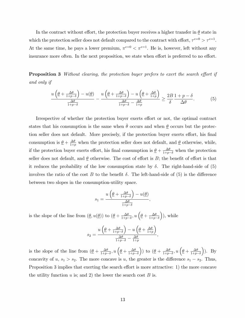
In the contract without effort, the protection buyer receives a higher transfer in θ state in

which the protection seller does not default compared to the contract with effort, τ e=0 > τ e=1.

At the same time, he pays a lower premium, πe=0 < πe=1. He is, however, left without any

insurance more often. In the next proposition, we state when effort is preferred to no effort.

Proposition 3 Without clearing, the protection buyer prefers to exert the search effort if

and only if

u(θ + ∆θ

1+p−δ

)− u(θ)

∆θ1+p−δ

−u(θ + ∆θ

1+p−δ

)− u

(θ + ∆θ

1+p

)∆θ

1+p−δ −∆θ1+p

≥ 2B

δ

1 + p− δ∆θ

. (5)

Irrespective of whether the protection buyer exerts effort or not, the optimal contract

states that his consumption is the same when θ occurs and when θ occurs but the protec-

tion seller does not default. More precisely, if the protection buyer exerts effort, his final

consumption is θ + ∆θ1+p

when the protection seller does not default, and θ otherwise, while,

if the protection buyer exerts effort, his final consumption is θ + ∆θ1+p−δ when the protection

seller does not default, and θ otherwise. The cost of effort is B; the benefit of effort is that

it reduces the probability of the low consumption state by δ. The right-hand-side of (5)

involves the ratio of the cost B to the benefit δ. The left-hand-side of (5) is the difference

between two slopes in the consumption-utility space.

s1 =u(θ + ∆θ

1+p−δ

)− u(θ)

∆θ1+p−δ

,

is the slope of the line from (θ, u(θ)) to (θ + ∆θ1+p−δ , u

(θ + ∆θ

1+p−δ

)), while

s2 =u(θ + ∆θ

1+p−δ

)− u

(θ + ∆θ

1+p

)∆θ

1+p−δ −∆θ1+p

,

is the slope of the line from (θ + ∆θ1+p−δ , u

(θ + ∆θ

1+p−δ

)) to (θ + ∆θ

1+p−δ , u(θ + ∆θ

1+p−δ

)). By

concavity of u, s1 > s2. The more concave is u, the greater is the difference s1 − s2. Thus,

Proposition 3 implies that exerting the search effort is more attractive: 1) the more concave

the utility function u is; and 2) the lower the search cost B is.

13

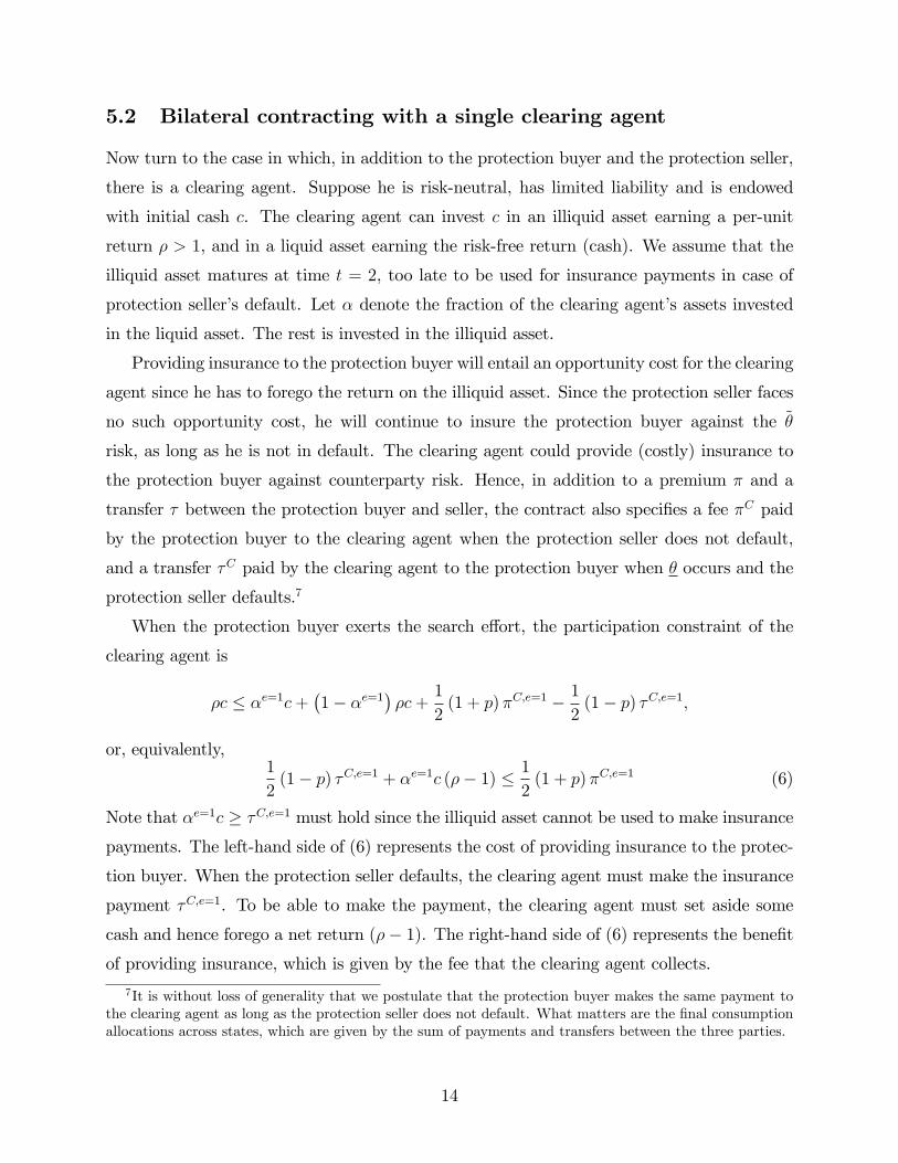
5.2 Bilateral contracting with a single clearing agent

Now turn to the case in which, in addition to the protection buyer and the protection seller,

there is a clearing agent. Suppose he is risk-neutral, has limited liability and is endowed

with initial cash c. The clearing agent can invest c in an illiquid asset earning a per-unit

return ρ > 1, and in a liquid asset earning the risk-free return (cash). We assume that the

illiquid asset matures at time t = 2, too late to be used for insurance payments in case of

protection seller’s default. Let α denote the fraction of the clearing agent’s assets invested

in the liquid asset. The rest is invested in the illiquid asset.

Providing insurance to the protection buyer will entail an opportunity cost for the clearing

agent since he has to forego the return on the illiquid asset. Since the protection seller faces

no such opportunity cost, he will continue to insure the protection buyer against the θ

risk, as long as he is not in default. The clearing agent could provide (costly) insurance to

the protection buyer against counterparty risk. Hence, in addition to a premium π and a

transfer τ between the protection buyer and seller, the contract also specifies a fee πC paid

by the protection buyer to the clearing agent when the protection seller does not default,

and a transfer τC paid by the clearing agent to the protection buyer when θ occurs and the

protection seller defaults.7

When the protection buyer exerts the search effort, the participation constraint of the

clearing agent is

ρc ≤ αe=1c+(1− αe=1

)ρc+

1

2(1 + p) πC,e=1 − 1

2(1− p) τC,e=1,

or, equivalently,1

2(1− p) τC,e=1 + αe=1c (ρ− 1) ≤ 1

2(1 + p) πC,e=1 (6)

Note that αe=1c ≥ τC,e=1 must hold since the illiquid asset cannot be used to make insurance

payments. The left-hand side of (6) represents the cost of providing insurance to the protec-

tion buyer. When the protection seller defaults, the clearing agent must make the insurance

payment τC,e=1. To be able to make the payment, the clearing agent must set aside some

cash and hence forego a net return (ρ− 1). The right-hand side of (6) represents the benefit

of providing insurance, which is given by the fee that the clearing agent collects.

7It is without loss of generality that we postulate that the protection buyer makes the same payment tothe clearing agent as long as the protection seller does not default. What matters are the final consumptionallocations across states, which are given by the sum of payments and transfers between the three parties.

14

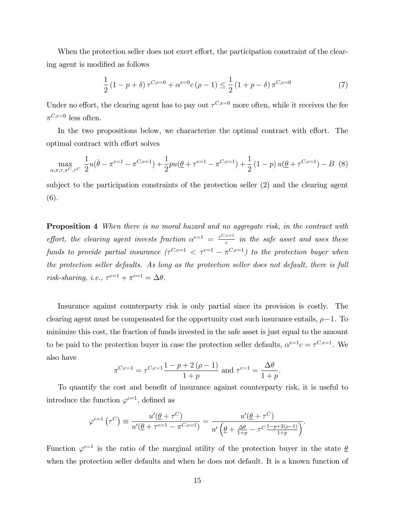
When the protection seller does not exert effort, the participation constraint of the clear-

ing agent is modified as follows

1

2(1− p+ δ) τC,e=0 + αe=0c (ρ− 1) ≤ 1

2(1 + p− δ) πC,e=0 (7)

Under no effort, the clearing agent has to pay out τC,e=0 more often, while it receives the fee

πC,e=0 less often.

In the two propositions below, we characterize the optimal contract with effort. The

optimal contract with effort solves

maxα,π,τ ,πC ,τC

1

2u(θ− πe=1− πC,e=1) +

1

2pu(θ+ τ e=1− πC,e=1) +

1

2(1− p)u(θ+ τC,e=1)−B (8)

subject to the participation constraints of the protection seller (2) and the clearing agent

(6).

Proposition 4 When there is no moral hazard and no aggregate risk, in the contract with

effort, the clearing agent invests fraction αe=1 = τC,e=1

cin the safe asset and uses these

funds to provide partial insurance (τC,e=1 < τ e=1 − πC,e=1) to the protection buyer when

the protection seller defaults. As long as the protection seller does not default, there is full

risk-sharing, i.e., τ e=1 + πe=1 = ∆θ.

Insurance against counterparty risk is only partial since its provision is costly. The

clearing agent must be compensated for the opportunity cost such insurance entails, ρ−1. To

minimize this cost, the fraction of funds invested in the safe asset is just equal to the amount

to be paid to the protection buyer in case the protection seller defaults, αe=1c = τC,e=1. We

also have

πC,e=1 = τC,e=1 1− p+ 2 (ρ− 1)

1 + pand τ e=1 =

∆θ

1 + p.

To quantify the cost and benefit of insurance against counterparty risk, it is useful to

introduce the function ϕe=1, defined as

ϕe=1(τC)≡ u′(θ + τC)

u′(θ + τ e=1 − πC,e=1)=

u′(θ + τC)

u′(θ + ∆θ

1+p− τC 1−p+2(ρ−1)

1+p

) .Function ϕe=1 is the ratio of the marginal utility of the protection buyer in the state θ

when the protection seller defaults and when he does not default. It is a known function of

15

exogenous variables and τC , and it is decreasing in τC . Since insurance against counterparty

risk is only partial, ϕ is greater than one. Higher insurance against counterparty default

(higher τC) reduces ϕ, moving the marginal utilities closer to one, i.e., closer to full insurance.

The following proposition characterizes the optimal degree of counterparty risk insurance in

the contract with effort.

Proposition 5 When there is no moral hazard and no aggregate risk, if ϕe=1 (0) ≤ 1+ 2(ρ−1)1−p ,

then the clearing agent is not used. Otherwise, if

ϕe=1 (c) > 1 +2 (ρ− 1)

1− p , (9)

then α∗ = 1, while if (9) does not hold, τC is given by

ϕe=1(τC)

= 1 +2 (ρ− 1)

1− p . (10)

The optimal degree of insurance balances benefits of insurance against counterparty risk

(left-hand side of (10)) with the opportunity cost of holding cash reserves (right-hand side

of (10)). If the opportunity cost of cash reserves is very high (ρ − 1 is high), there will be

less insurance. As the probability of counterparty default (1 − p) rises, the transfer is theevent of default increases. Indeed, when counterparty default is frequent, it is worthy to put

a high amount of assets in cash reserves to pay τC,e=1.

The optimal contract without effort solves

maxα,π,τ ,πC ,τC

1

2u(θ−πe=0−πC,e=0) +

1

2(p− δ)u(θ+ τ e=0−πC,e=0) +

1

2(1− p+ δ)u(θ+ τC,e=0)

(11)

subject to the participation constraints of the protection seller (4) and the clearing agent

(7). Next, we state two propositions characterizing the optimal contract without effort.

Proposition 6 When there is no moral hazard and no aggregate risk, in the contract without

effort, the clearing agent provides partial insurance (τC,e=0 < τ e=0−πC,e=0) to the protection

buyer when the protection seller defaults. As long as the protection seller does not default,

there is full risk-sharing, i.e., τ e=0 + πe=0 = ∆θ.

16

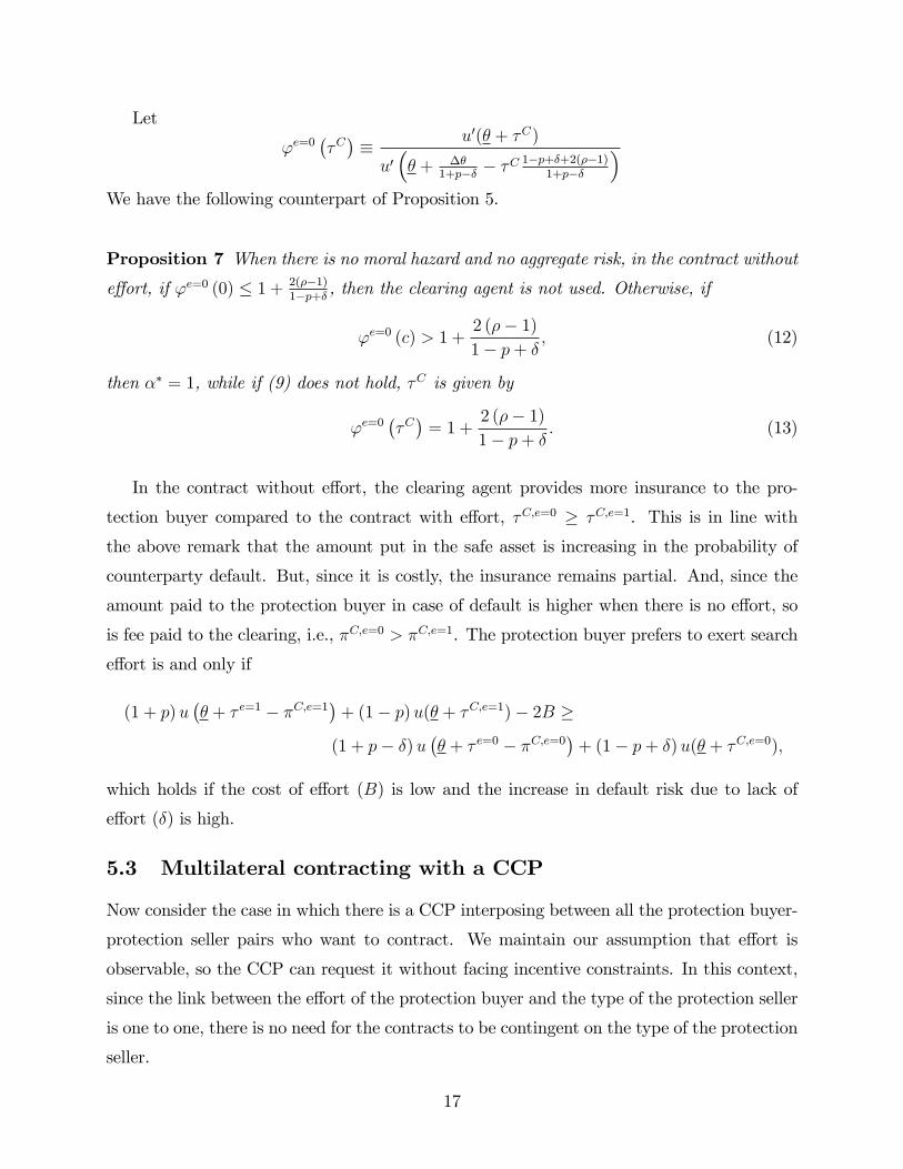
Let

ϕe=0(τC)≡ u′(θ + τC)

u′(θ + ∆θ

1+p−δ − τC1−p+δ+2(ρ−1)

1+p−δ

)We have the following counterpart of Proposition 5.

Proposition 7 When there is no moral hazard and no aggregate risk, in the contract without

effort, if ϕe=0 (0) ≤ 1 + 2(ρ−1)1−p+δ , then the clearing agent is not used. Otherwise, if

ϕe=0 (c) > 1 +2 (ρ− 1)

1− p+ δ, (12)

then α∗ = 1, while if (9) does not hold, τC is given by

ϕe=0(τC)

= 1 +2 (ρ− 1)

1− p+ δ. (13)

In the contract without effort, the clearing agent provides more insurance to the pro-

tection buyer compared to the contract with effort, τC,e=0 ≥ τC,e=1. This is in line with

the above remark that the amount put in the safe asset is increasing in the probability of

counterparty default. But, since it is costly, the insurance remains partial. And, since the

amount paid to the protection buyer in case of default is higher when there is no effort, so

is fee paid to the clearing, i.e., πC,e=0 > πC,e=1. The protection buyer prefers to exert search

effort is and only if

(1 + p)u(θ + τ e=1 − πC,e=1

)+ (1− p)u(θ + τC,e=1)− 2B ≥

(1 + p− δ)u(θ + τ e=0 − πC,e=0

)+ (1− p+ δ)u(θ + τC,e=0),

which holds if the cost of effort (B) is low and the increase in default risk due to lack of

effort (δ) is high.

5.3 Multilateral contracting with a CCP

Now consider the case in which there is a CCP interposing between all the protection buyer-

protection seller pairs who want to contract. We maintain our assumption that effort is

observable, so the CCP can request it without facing incentive constraints. In this context,

since the link between the effort of the protection buyer and the type of the protection seller

is one to one, there is no need for the contracts to be contingent on the type of the protection

seller.

17

Because all random variables are i.i.d, the aggregate mass of defaults is deterministic.

For the sake of comparability with the single clearing agent case, we assume that the CCP is

initially endowed with wealth c, which it can invest in an illiquid project with time 2 return

ρ > 1. The total amount of insurance transfers to be paid by the CCP at time t = 1 is∫ 1

i=0

1(θi = θ)1(Ri = 0)τCdi, (14)

where 1 denotes the indicator variable, and i indexes the protection buyer-protection seller

pairs. Because the θi and Ri are independent, by the law of large numbers (14) is equal to

1

2(1− p)τC

if protection buyers exert search effort and it is equal to

1

2(1− p+ δ)τC

if protection buyers do not exert effort.

The participation constraint of the CCP is

1

2(1− p) τC + αc (ρ− 1) ≤ 1

2(1 + p) πC (15)

if effort is exerted and

1

2(1− p+ δ) τC + αc (ρ− 1) ≤ 1

2(1 + p− δ) πC (16)

otherwise.

The participation constraints of the CCP (15) and (16) bind (by the same logic as in the

previous subsection). Note that any α > 0 tightens the participation constraint due to the

opportunity cost of cash reserves. This yields the following proposition:

Proposition 8 When there is no moral hazard and no aggregate risk, the CCP optimally

sets α = 0. The fees are given by

πC,e=1 =1− p1 + p

τC,e=1

if the search effort is exerted,and

πC,e=0 =1− p+ δ

1 + p− δ τC,e=0

otherwise.

18

Proposition 8 states that the CCP can collect the fees such that they exactly cover the

insurance payments. Hence, unlike the single clearing agent, the CCP does not need to

set aside cash reserves and incur the corresponding opportunity cost. Since there is no

opportunity cost of providing insurance, the next proposition shows that it is optimal for

the CCP to provide full insurance to the protection buyers, regardless of whether or not the

effort is exerted.

Proposition 9 When there is no moral hazard and no aggregate risk, the CCP provides full

insurance against counterparty default risk, regardless of whether or not the search effort is

exerted. It is hence optimal for the protection buyers to economize on search costs and never

exert effort. In this first-best allocation, the aggregate default rate is higher than without the

CCP.

With the CCP, all idiosyncratic risk can be mutualized. Consequently, when there is no

aggregate risk, protection buyers are fully insured. Hence, there is no need to exert effort to

find creditworthy counterparties and no-effort is optimal. This underscores that, in spite of

formal similarities, the setup we consider is very different from that analyzed by Holmström

and Tirole (1998).

• In Holmström and Tirole (1998), at a cost B, the agent can reduce the probability

of low output. Thus, effort increases the average output in the economy. Even with

risk-neutrality this can be valuable, if B is low enough.

• In the present model, at a cost B, the agent can find a protection seller with lowprobability of default. But, effort does not increase the average output in the economy:

the overall output of the protection sellers is exogenous and unaffected by the protection

buyers’efforts. Therefore, the effort of the protection buyers can be useful only if it

increases their risk-sharing ability. However, with mutualization and no aggregate-risk,

full risk-sharing can be achieved even if the protection sellers are bad. Hence, effort is

not optimal.

Thus, while the CCP achieves the first-best, it can at the same time increase aggregate

default risk. This is not a symptom of a market failure, however. Rather, it is a feature of

the first-best.

19

Finally, note that with all idiosyncratic risk mutualized by the CCP, it is no longer

strictly necessary for protection sellers to be a part of the risk-sharing transaction. Risk-

mutualization among protection buyers is enough. This differs from the environment with

aggregate risk, in which risk-mutualization by protection buyers is not enough to deliver

full insurance. In that case, as we show in the next section, sellers play an important role

even with the CCP mutualizing the idiosyncratic risk. Therefore, the effort of the protection

buyers to search for good protection sellers can be beneficial as it increases the resources

available to insure against aggregate risk.

6 Aggregate risk and observable effort

6.1 Aggregate risk

We now study the optimal design of the CCP when there is aggregate risk, but still no

moral hazard. To extend our analysis to the case of aggregate risk, our set-up is modified as

follows. There are two aggregate states in the economy, high and low, each occurring with

equal probability. In the high state, the probability of θ is 12

+ γ, while the probability of θ

is 12− γ. In the low state, the probability of θ is 1

2− γ, while the probability of θ is 1

2+ γ.

Conditional on the macro-state, the realizations of the θj are i.i.d. Note that, ex-ante, the

two values θ and θ are equiprobable, as in the analysis of the previous sections. But, ex-post,

after observing the macro-state, one of them becomes more likely. When γ = 0 there is no

macro-risk and agents are only exposed to idiosyncratic risk. At the other extreme, when

γ = 12, there is no idiosyncratic risk, and, in each of the two macro-states, the values of

all the assets of all the protection sellers are the same. We now consider the case in which

γ ∈ (0, 12) and there is combination of aggregate and idiosyncratic risk. We also assume that

pR >∆θ

2> (p− δ)R, (17)

which implies that, if all protection buyers contract with creditworthy protection sellers,

the total resources brought to the table by all the parties are suffi cient to fully insure the

protection buyers, while, if the protection buyers fail to exert effort, full insurance may be

infeasible. Finally, to focus on the effects of aggregate risk in the simplest possible set-up,

we assume that the CCP does not have any cash endowment, c = 0.

The macro-state is realized at time 34, after the market infrastructure and the contracts

20

have been designed and effort has been exerted. The realization of the macro-state is publicly

observable, and contracts are contingent upon it. Let(π, τ , πC , τC

)denote fees and transfers

in the high state and let(π, τ , πC , τC

)denote fees and transfers in the low state.

6.2 Optimal clearing and contracting with effort

Consider first the contract with effort. The objective function of the protection buyer under

effort is given by

1

2

[(1

2+ γ

)u(θ − πe=1 − πC,e=1) +

(1

2− γ)pu(θ + τ e=1 − πC,e=1)+ (18)(

1

2− γ)

(1− p)u(θ + τC,e=1)−B]

+1

2

[(1

2− γ)u(θ − πe=1 − πC,e=1)+(

1

2+ γ

)pu(θ + τ e=1 − πC,e=1) +

(1

2+ γ

)(1− p)u(θ + τC,e=1)−B

]The participation constraint of the protection seller is(

1

2+ γ

)πe=1 +

(1

2− γ)p(−τ e=1

)+

(1

2− γ)πe=1 +

(1

2+ γ

)p(−τ e=1

)≥ 0 (19)

As before, the CCP will collect the fees such that they exactly cover the insurance payments

in each state so that(1

2− γ)

(1− p) τC,e=1 =

[1

2+ γ +

(1

2− γ)p

]πC,e=1

in the high state and(1

2+ γ

)(1− p) τC,e=1 =

[1

2− γ +

(1

2+ γ

)p

]πC,e=1

in the low state. Hence, we have that

πC,e=1 =

(12− γ)

(1− p) τC,e=1

12

(1 + p) + γ (1− p)and πC,e=1 =

(12

+ γ)

(1− p) τC,e=1

12

(1 + p)− γ (1− p)(20)

As shown in the appendix, this yields the following proposition.

Proposition 10 With aggregate risk but no moral hazard, the optimal contract with central-

ized clearing and effort provides full insurance to the protection buyers, and their expected

utility is

u(E[θ])−B. (21)

21

When the protection seller does not default, transfers are

τ e=1 =1

12

(1 + p)− γ (1− p)∆θ

2>

112

(1 + p) + γ (1− p)∆θ

2= τ e=1, (22)

while in case of default they are

τC,e=1 = τC,e=1 =∆θ

2. (23)

(23) is a direct implication of full risk sharing. (22) is a direct implication of (23),

(20) and the fact that the consumption of the protection buyer is the same whether the

protection seller defaults or not. Furthermore, feasibility requires that the transfer paid by

the protection seller when he does not default (τ e=1) be lower than his resources (R). Thus,

in the optimal contract we have

R > τ e=1 =1

12

(1 + p)− γ (1− p)1

2∆θ. (24)

Since the right-hand side of (24) is increasing in γ, and maximum γ is 12, a suffi cient condition

for feasibility is pR > ∆θ2which holds by (17).

(21) is identical to its counterpart without aggregate risk. (17) implies that, under

effort, the population of protection sellers brings enough resources to the table to provide

full insurance to the protection buyers. Since they are competitive and risk-neutral, the

protection sellers are willing to do that as long as they break even on average. Thus, insurance

comes at no cost, except the search cost B. Otherwise stated, if aggregate risk is relatively

small, and when protection buyers exert effort, optimal risk sharing can be provided within

the CCP. The main difference between this result and that of the previous section is that,

without aggregate risk, effort and protection sellers were not needed for full risk-sharing.

This is no longer the case with aggregate risk.

6.3 Optimal clearing and contracting without effort

Now consider the contract without effort. The objective function of the protection buyer

without effort is given by

1

2

[(1

2+ γ

)u(θ − πe=0 − πC,e=0) +

(1

2− γ)

(p− δ)u(θ + τ e=0 − πC,e=0)+ (25)(1

2− γ)

(1− p+ δ)u(θ + τC,e=0)

]+

1

2

[(1

2− γ)u(θ − πe=0 − πC,e=0)+(

1

2+ γ

)(p− δ)u(θ + τ e=0 − πC,e=0) +

(1

2+ γ

)(1− p+ δ)u(θ + τC,e=0)

]22

The participation constraint of the protection seller is(1

2+ γ

)πe=0 +

(1

2− γ)

(p− δ)(−τ e=0

)+

(1

2− γ)πe=0 +

(1

2+ γ

)(p− δ)

(−τ e=0

)≥ 0

(26)

As before, the CCP will collect the fees such that they exactly cover the insurance payments

in each state so that(1

2− γ)

(1− p+ δ) τC,e=0 =

[1

2+ γ +

(1

2− γ)

(p− δ)]πC,e=0

in the high state and(1

2+ γ

)(1− p+ δ) τC,e=0 =

[1

2− γ +

(1

2+ γ

)(p− δ)

]πC,e=0

in the low state. Hence, we have that

πC,e=0 =

(12− γ)

(1− p+ δ) τC,e=0

12

(1 + p− δ) + γ (1− p+ δ)and πC,e=0 =

(12

+ γ)

(1− p+ δ) τC,e=0

12

(1 + p− δ)− γ (1− p+ δ)(27)

These equations are the same as those we had with effort, except that here the cost B is not

incurred and the probability of counterparty default is raised by δ.

Thus, we can state the following proposition.

Proposition 11 With aggregate risk but no moral hazard, if

R ≥ 112

(1 + p− δ)− γ (1− p+ δ)

∆θ

2(28)

holds, then the optimal contract with the CCP and without effort provides full insurance to

the protection buyers, with transfers in the event of default τC,e=0 = τC,e=0 = ∆θ2. If (28) does

not hold, then there is full risk-sharing in the high aggregate state. But in the low aggregate

state, the amount of insurance is limited by the resource constraint, so that τC,e=0 > τC,e=0.

(28) is the counterpart of (24) in the case with no effort. To understand the economic

forces driving the result in Proposition 11, it is useful to first consider the extreme case with

only macro risk (γ = 12). In that case, (28) becomes

p− δ > ∆θ

2,

which, by (17), does not hold. For less extreme cases, the right-hand-side of (28) is increasing

in γ, which measures the extent of aggregate risk. When aggregate risk is large (i.e., when

23

γ is large), if the protection buyers don’t exert effort, the amount of resources in the bad

macro-state is insuffi cient to provide full risk-sharing, even with a CCP.

If (28) holds so that full risk-sharing is feasible, the expected utility in the contract

without effort is

u(E[θ])

(29)

Comparing (21) and (29), it follows that whenever (28) holds, protection buyers will choose

not to exert search effort since they can get full insurance while saving on the search cost B.

Note that if γ = 0 and there is no aggregate risk, condition (28) is equivalent to R ≥ ∆θ1+p−δ

which is always satisfied since we assume R > ∆θ. That is, for γ = 0, full risk-sharing is

feasible when effort is not exerted. Hence, exerting effort is not optimal (see Proposition 9).

As mentioned above, for γ = 12, condition (28) is equivalent to (p− δ)R ≥ ∆θ

2which

cannot hold due to (17). That is, when effort is not exerted and γ = 12, full risk-sharing is

not feasible. We can state the following proposition for this special case.

Proposition 12 With aggregate risk, no moral hazard and no idiosyncratic risk, γ = 12, the

optimal contract has πe=0 = (p− δ)R, τ e=0 = R and τC,e=0 = (p− δ)R. Protection buyersprefer to exert the search effort if and only if

u(E[θ])−B ≥ 1

2u(θ − (p− δ)R

)+

1

2u (θ + (p− δ)R) . (30)

Condition (30) is more likely to hold: 1) the smaller B; 2) the smaller p− δ; 3) the moreconcave u. Since the right-hand side of (28) is increasing in γ, there exists γ∗ such that for

all γ > γ∗, condition (28) does not hold. We have that

γ∗ =1 + p− δ − ∆θ

R

2 (1− p+ δ)(31)

If aggregate risk is limited, in the sense that γ ≤ γ∗, exerting effort is not optimal, since full

risk-sharing can be obtained without effort. But if aggregate risk is large, in the sense that

γ > γ∗, then exerting effort is preferred to not exerting effort if the expected utility under

effort (21) is higher than the expected utility in the contract without effort and with partial

insurance. The latter is given by:

1

2u(θ + τC,e=0)

[1 +

(1

2− γ)]

+1

2

[(1

2+ γ

)(p− δ)u(θ + τ e=0 − πC,e=0)+(

1

2+ γ

)(1− p+ δ)u(θ + τC,e=0)

].

24

Suppose γ > γ∗ and protection buyers choose not to exert effort ex ante. One might

wonder why, if the low state is realized, protection buyers do not search for good protection

sellers ex post? This is because, after the low state is realized, it’s too late to share the

macro-risk. Effort in our set-up enhances the risk-sharing capacity, but this can only be

done ex ante, before the resolution of uncertainty.

7 Aggregate risk and moral hazard

We now turn to the case in which effort is unobservable. We first assume that a benevolent

CCP can optimally design all the transfers and fees(π, τ , πC , τC

)to maximize the expected

utility of protection buyers. We then consider the case in which the CCP sets πC and τC ,

while the protection buyers set π and τ .

7.1 When the benevolent CCP sets the transfers

Suppose that a benevolent CCP can optimally design all the state-contingent transfers and

fees(π, τ , πC , τC

)to maximize the expected utility of protection buyers. Consider first the

contract with effort. Focus on the values of γ such that it would be optimal to exert effort

if it were observable (as spelled out in the previous section). If, for a given(π, τ , πC , τC

), a

protection buyer exerts effort, his payoff is given by

1

2

[(1

2+ γ

)u(θ − π − πC) +

(1

2− γ)pu(θ + τ − πC)+ (32)(

1

2− γ)

(1− p)u(θ + τC)−B]

+1

2

[(1

2− γ)u(θ − π − πC)+(

1

2+ γ

)pu(θ + τ − πC) +

(1

2+ γ

)(1− p)u(θ + τC)−B

]If a protection buyer does not exert effort, his payoff is given by

1

2

[(1

2+ γ

)u(θ − π − πC) +

(1

2− γ)

(p− δ)u(θ + τ − πC)+ (33)(1

2− γ)

(1− p+ δ)u(θ + τC)

]+

1

2

[(1

2− γ)u(θ − π − πC)+(

1

2+ γ

)(p− δ)u(θ + τ − πC) +

(1

2+ γ

)(1− p+ δ)u(θ + τC)

]Note that the contract cannot be contingent on effort, since the latter is unobservable.

Comparing (32) and (33), a protection buyer will prefer to exert unobservable effort if(1

2− γ)[

u(θ + τ − πC)− u(θ + τC)]

+

(1

2+ γ

)[u(θ + τ − πC)− u(θ + τC)

]≥ 2B

δ(34)

25

Suppose the CCP offers the same contract as that characterized in Proposition 10, so

that a protection buyer obtains full insurance. Then, τ − πC = τC and τ −πC = τC , and the

protection buyer will prefer to save on the search cost B and not exert effort. This will lead

to high (and socially suboptimal) default rates. Hence, we can state the following lemma.

Lemma 1 When the CCP offers full insurance against counterparty risk, unobservable effort

is not exerted. Hence, to induce effort, the incentive constraint (34) must bind and the CCP

provides only partial insurance against counterparty default risk.

We now solve for the second-best contract with effort. The classic tradeoff between

incentives and insurance arises. Incentive-compatibility requires that the protection buyer

remain exposed to some protection seller default risk.

The program of a benevolent CCP is to maximize (32) subject to the incentive constraint

(34), the participation constraint of the protection seller (19) and the CCP fees (20). We

can now state the following proposition.

Proposition 13 With aggregate risk and moral hazard, consumption is no longer equalized

across states in the optimal contract inducing effort. Thus,

θ + τ − πC = θ + τ − πC > θ − π − πC = θ − π − πC > θ + τC = θ + τC , (35)

and the optimal transfers and fees π, τ , πC , πC and τC are given by:

u(θ + τ − πC)− u(θ + τC) =2B

δ,

π = pτ − 2γ (1− p) τC12

(1 + p)− γ (1− p),

u(θ + τC)

u(θ + τ − πC)=

(1− p) u(θ − π − πC)

u(θ + τ − πC)− pu(θ − π − πC),

πC =

(12− γ)

(1− p)12

(1 + p) + γ (1− p)τC and πC =

(12

+ γ)

(1− p)12

(1 + p)− γ (1− p)τC .

In the first-best, the protection buyer gets full insurance when he exerts search effort so

that θ+ τ − πC = θ− π− πC = θ+ τC . By (35), this is no longer the case with moral hazard.

The intuition is as follows. As stated in Lemma 1, to ensure that the protection buyer exerts

26

effort, he must be exposed to some counterparty risk so that there must be a wedge between

θ + τ − πC and θ + τC . Such a wedge can be obtained either by raising θ + τ − πC or bylowering θ + τC . The latter is more costly since the consumption of the protection buyer is

minimal when θ is realized and the protection seller defaults. Hence, the former is preferred.

Since raising τ requires an increase in π, we have θ + τ − πC > θ − π − πC .The optimal contract without effort is as characterized in Proposition 11. Protection

buyers prefer the contract with effort if and only if their expected utility under effort is

higher than their expected utility without effort. Since the expected utility in the optimal

contract with effort is necessarily lower under moral hazard compared to the first-best, while

the expected utility without effort is the same as in the first-best, we have the following

proposition.

Proposition 14 The set of parameters for which the optimal contract mandates effort is

smaller under moral hazard than when effort is observable.

For completeness, we state a condition under which the benevolent CCP chooses to offer

the contract inducing search effort for the special case when γ = 12.

Proposition 15 With moral hazard, aggregate risk and no idiosyncratic risk, γ = 12, the

CCP offers the contract inducing search effort by the protection buyers if and only if

1

2u(θ − π) +

1

2u(θ + τC) +

p− δδ

B ≥ 1

2u(θ − (p− δ)R

)+

1

2u (θ + (p− δ)R) . (36)

7.2 When the parties set the terms of their contracts

Having analyzed the optimal contract designed by the CCP, we now consider the case in

which the CCP sets πC and τC , while the protection buyers set π and τ . That is, expect-

ing state-contingent premia πe and transfers τ e, the benevolent CCP chooses fees πC and

transfers τC to maximize the expected utility of the protection buyer subject to relevant

constraints. Rational expectations require that the protection buyer does choose the premia

and transfers expected by the CCP. We now argue that the rational expectations condition

will be satisfied in the optimal contracts designed by the CCP.

27

Consider first the case when the benevolent CCP chooses to offer the contract without

effort since it yields a higher expected utility than the contract with effort. Given πC,e=0

and τC,e=0, if the protection buyer decides not to do effort, he will choose the same πe=0 and

τ e=0 as the ones chosen by the CCP since this is the best contract without effort. Would

the protection buyer choose to do effort, given πC,e=0 and τC,e=0? No, since even the best

contract with effort is dominated by the contract without effort in this case. Hence, the

rational expectations condition is satisfied.

Now consider the case when the benevolent CCP chooses to offer the contract inducing

unobservable effort since it yields a higher expected utility than the contract without effort.

By the same logic as in the previous case, a protection buyer cannot do better by deviating

from π and τ from the optimal contract with effort.

Thus, to implement the second-best, it is enough that the CCP sets optimally its fees

and the amount of insurance against counterparty default. Once it has done that, the best

response of the contracting parties will yield the optimal contract.

8 Conclusion

We analyze three ways in which counterparty risk can be mitigated.

• Trading parties can deposit resources in safe assets, and these resources can be usedto make promised payments in case the counterparty defaults. This is comparable to

self-insurance, whereby an agent saves to insure against future negative shocks.

• Trading parties can exert effort to find creditworthy counterparties, whose counterpartydefault risk is low. This is comparable to self-protection, whereby an agent exerts effort

to reduce damage probabilities.

• Finally, trading parties can mutualize their risk.

We show that an appropriately designed centralized clearing mechanism enables the trad-

ing parties to benefit from the mutualization of (the idiosyncratic component of) risk, and

therefore dominates no-clearing or decentralized clearing. But we also warn that such an

arrangement has limitations:

28

• First, risk-mutualization is effective only to deal with idiosyncratic risk. It leaves thetrading parties exposed to aggregate risk. Dealing with that risk can require that

agents exert effort to search for solid, creditworthy counterparties.

• Second, risk-mutualization can weaken the incentives of the trading parties to exertsuch search effort. When effort is unobservable, i.e., when there is moral hazard, the

CCP must be designed to maintain the incentives to search for solid counterparties.

This requires that the agents keep some exposure to the risk that their counterparty

will default.

We thus uncover a tradeoff between i) the ability of the system to withstand aggregate

shocks (which requires that incentives be maintained), and ii) the extent to which risk can be

mutualized in a CCP. To complement these insights and offer a more complete set of policy

implications, it would interesting to explore the following avenues for further research:

Governance: The analysis above spells out the optimal design of the CCP, maximizing

the expected utility of protection buyers, subject to the participation, incentive and feasibility

constraints of the different parties. In practice, who would perform and implement this

design, and thus set up a socially optimal CCP?

CCPs are, in a sense, utilities, providing services to financial institutions. Such utilities

are often structured as cooperatives, or mutuals, whose members are both owners and users.

Consider a mutual CCP, whose members would be the protection buyers. Its objective and

constraints would be those analyzed above, and it would therefore implement the optimal

CCP we characterized. In contrast, consider a for-profit, shareholder-owned CCP. Its ob-

jective, the maximization of profit, would not necessarily coincide with the maximization of

social welfare. We have shown above that, in presence of moral hazard, the CCP should

expose its members to some counterparty risk, to maintain their incentives. Suppose that

the for-profit CCP did not do that and offered full insurance. Then, if the protection buyers

believed the CCP would indeed deliver full insurance, they would not exert search effort,

and they would also be willing to pay large fees. In the good macro-state, the CCP would

use part of these fees to pay insurance, and the remaining part would be profits. In the

bad macro-state, the rate of counterparty failures would be large and the CCP would go

bankrupt. But, to the extent that a large population of protection buyers would operate

within the CCP, this bankruptcy would be a systemic event. The government would have to

29

step in and bail out the protection buyers, thus confirming their initial expectation that full

insurance would actually be provided. Thus, CCPs managed as for-profit organizations may

be prone to gambling and generate systemic risk. To avoid this outcome, they should be

regulated. In particular their capital should be large enough to absorb counterparty defaults,

so that government bail outs would not be needed.

Risk control and management by the CCP: In the analysis above, the CCP

controls counterparty risk only indirectly, via the incentives of the protection buyers. But

the CCP could also exert effort to directly gauge the creditworthiness of the protection sellers.

This could mitigate the moral hazard problem analyzed above and improve risk-sharing.

Competition: Consider the case in which a benevolent CCP would seek to maintain

the incentives of the protection buyers by exposing them to some idiosyncratic risk. Could

the protection buyers undo this by acquiring the remaining insurance from another clearing

entity? This suggests that exclusivity could be needed to implement the second-best. In that

sense the CCP would be a natural monopoly. Of course, in that case, the CCP should be

regulated, to avoid excessively high fees. Again, the mutual structure, which gives ownership

and control rights to users, could prove useful in this context.

30

References

Acharya, V. and A. Bisin, 2010, “Counterparty Risk Externality: Centralized versus

Over-the-counter Markets,”NBER working paper No. 17000.

Biais, B., F. Heider and M. Hoerova, 2010, “Risk-sharing or Risk-taking? Counterparty

Risk, Incentives and Margins,”working paper, Toulouse School of Economics and ECB.

Biais, B. and C. Casamatta (1999), “Optimal Leverage and Aggregate Investment,”Jour-

nal of Finance, 54(4), 1291-1323.

Biais, B., T. Mariotti, G. Plantin and J. C. Rochet, 2007, “Dynamic Security Design:

Convergence to Continuous Time and Asset Pricing Implications,”Review of Economic Stud-

ies, 74(2), 345-390.

Dewatripont and Tirole, 1993, The Prudential Regulation of Banks, MIT Press.

Darrell Duffi e and Haoxiang Zhu, 2011, “Does a Central Clearing Counterparty Reduce

Counterparty Risk?”Working paper, Stanford University

Ehrlich, I and G. becker, 1972, “Market insurance, self-insurance and self-protection,”

Journal of Political Economy, 623-648.

Freixas and Rochet, 2008, Microeconomics of Banking, MIT Press.

Froot, K., Scharfstein, D. and J. Stein, 1993, “RiskManagement: Coordinating Corporate

Investment and Financing Policies,”Journal of Finance, 48 (5), 1629-1658.

Froot, K. and J. Stein, 1998, “Risk Management, Capital Budgeting, and Capital Struc-

ture Policy for Financial Institutions: An Integrated Approach,”Journal of Financial Eco-

nomics, 47, 55-82.

Hanson, S., A. Kashyap and J. Stein, 2011, “A Macroprudential Approach to Financial

Regulation,”Journal of Economic Perspectives, 25 (1), 3-28.

Holmström, B. and J. Tirole, 1998, “Private and Public Supply of Liquidity,”Journal of

Political Economy, 106, 1-40.

Jensen, M., and Meckling, 1976, “Theory of the Firm: Managerial Behavior, Agency

Costs and Ownership Structure,”Journal of Financial Economics, 3 (4), 305-360.

Pirrong, C., 2011, “The Economics of Clearing in Derivatives Markets: Netting, Asym-

metric Information, and the Sharing of Default Risks Through a Central Counterparty,”

working paper, University of Houston.

Rochet, J. C. and J. Tirole, 1996, “Interbank Lending and Systemic Risk,”Journal of

Money Credit and Banking 28, 733-762.

31

Thompson, J.R., 2010, “Counterparty Risk in Financial Contracts: Should the Insured

Worry about the Insurer?,”Quarterly Journal of Economics, 125(3), 1195-1252.

Tirole, 2006, The Theory of Corporate Finance, Princeton University Press.

32

Appendix

Proof of Proposition 1 Let µ denote the Lagrange multiplier on the protection seller’s

participation constraint. The first-order conditions yield:

u′(θ − πe=1

)= µ = u′

(θ + τ e=1

).

Thus, the participation constraint binds, so that πe=1 = pτ e=1. Also, there is full risk-sharing

as long as the protection seller does not default, and τ e=1 + πe=1 = θ − θ ≡ ∆θ. But, the

protection buyer remains exposed to counterparty risk. QED

Proof of Proposition 2 Let µ denote the Lagrange multiplier on the protection seller’s

participation constraint. The first-order conditions yield:

u′(θ − πe=0

)= µ = u′

(θ + τ e=0

).

Thus, the participation constraint binds, so that πe=0 = (p− δ) τ e=0. Also, there is full

risk-sharing as long as the protection seller does not default, and τ e=0 + πe=0 = ∆θ. QED

Proof of Proposition 3 Expected utility of the protection buyer under effort is higher

than his expected utility under no effort if and only if

1

2u(θ − πe=1

)+

1

2pu(θ + τ e=1

)+

1

2(1− p)u(θ)−B ≥

1

2u(θ − πe=0

)+

1

2(p− δ)u

(θ + τ e=0

)+

1

2(1− p+ δ)u(θ)

or, equivalently,

(1 + p)u(θ + τ e=1

)− 2B ≥ (1 + p− δ)u

(θ + τ e=0

)+ δu(θ)

since there is full risk-sharing as long as the protection seller does not default.

Substituting for τ e=1 and τ e=0 from Propositions (1) and (2), respectively, we get

(1 + p)u

(θ +

∆θ

1 + p

)− 2B ≥ (1 + p− δ)u

(θ +

∆θ

1 + p− δ

)+ δu(θ)

or, after collecting terms and re-arranging,

u(θ + ∆θ

1+p−δ

)− u(θ)

∆θ1+p−δ

−u(θ + ∆θ

1+p−δ

)− u

(θ + ∆θ

1+p

)∆θ

1+p−δδ

1+p

≥ 2Bδ∆θ

1+p−δ

Note that the first terms is the slope of a line between u(θ) and u(θ + ∆θ

1+p−δ

), while the

second term is the slope of a line between u(θ + ∆θ

1+p

)and u

(θ + ∆θ

1+p−δ

). QED

33

Proof of Proposition 4 Let µ and µC denote the Lagrange multipliers on the protec-

tion seller’s and clearing agent’s participation constraints, respectively. Let µ0 and µ1 denote

the Lagrange multipliers on the feasibility constraints 0 ≤ α ≤ 1 and let µ2 be the Lagrange

multiplier on the feasibility constraint αc ≥ τC . The first-order conditions with respect to

π, τ , πC , τC and α (where we omit indexing by e = 1 everywhere) yield

u′(θ − π − πC) = µ (37)

u′(θ + τ − πC) = µ (38)

u(θ − π − πC) = µC (39)

(1− p)u′(θ + τC) = µC (1− p) + 2µ2 (40)

µC (ρ− 1) c = µ0 − µ1 + µ2c (41)

By (37) and (38), the participation constraint of the protection seller binds, π = pτ , and

there is full risk-sharing as long as the protection seller does not default, with τ = ∆θ1+p.

By (39), µC > 0 and the participation constraint of the clearing agent binds. By (37) and

(39), we have that µ = µC . Substituting into (40), we get

u′(θ + τC) = µ+2µ2

1− p

which, combined with (38), yields

θ + τC < θ + τ − πC

Hence, the clearing agent only provides a partial insurance against counterparty default.

Moreover, α > 0 must hold since otherwise the clearing agent cannot provide any insur-

ance against counterparty risk (as τC = 0 in this case). Hence, µ0 = 0. It follows from (41)

that µ2 > 0 must hold and α = τC

c. Since the participation constraint of the clearing agent

binds, we have that πC = τC 1−p+2(ρ−1)1+p

. QED

Proof of Proposition 5 Combining (40) and (41), we get:

u′(θ + τC)

u′(θ + τ − πC)=

2 (ρ− 1) + (1− p)(1− p) +

2µ1

(1− p) cu′(θ + τ − πC)

Substituting for τ and πC , we get

u′(θ + τC)

u′(θ + ∆θ

1+p− τC 1−p+2(ρ−1)

1+p

) = 1 +2 (ρ− 1)

1− p +2µ1

(1− p) cu′(θ + τ − πC)(42)

34

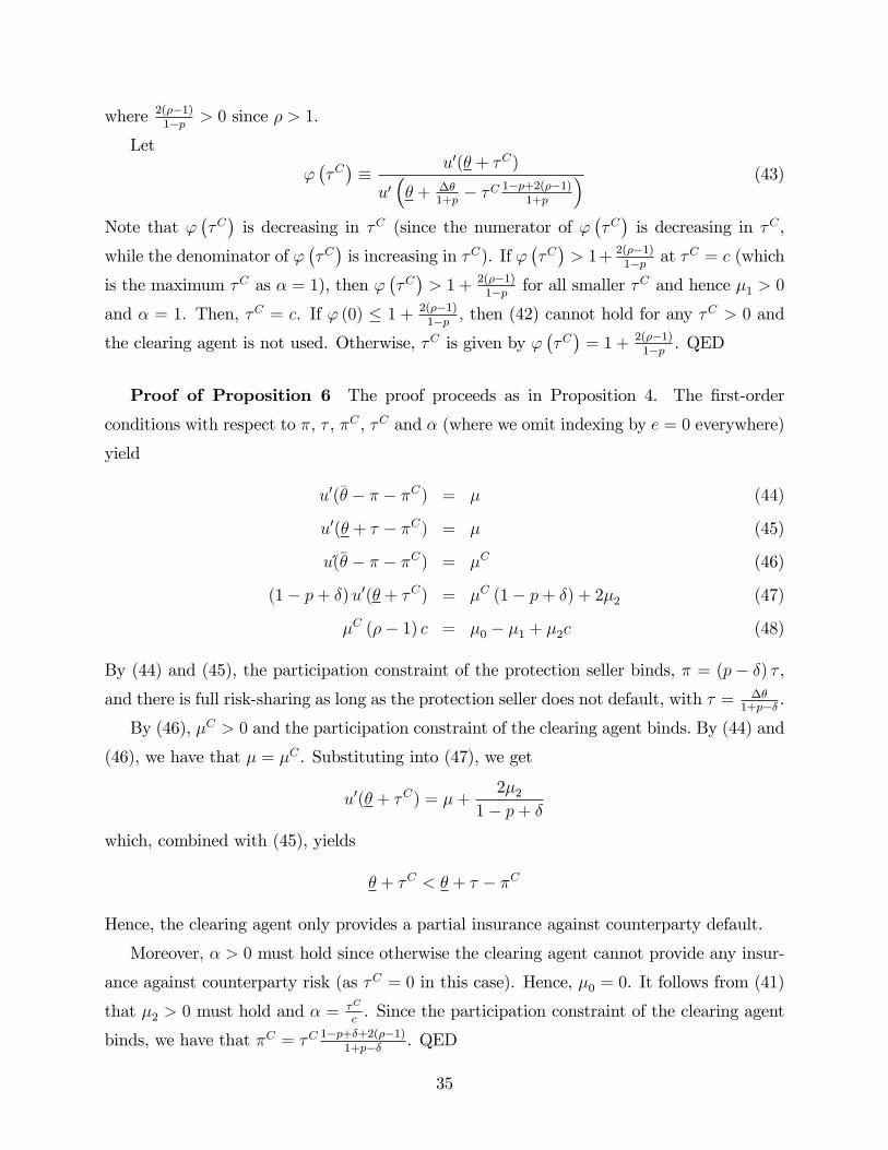
where 2(ρ−1)1−p > 0 since ρ > 1.

Let

ϕ(τC)≡ u′(θ + τC)

u′(θ + ∆θ

1+p− τC 1−p+2(ρ−1)

1+p

) (43)

Note that ϕ(τC)is decreasing in τC (since the numerator of ϕ

(τC)is decreasing in τC ,

while the denominator of ϕ(τC)is increasing in τC). If ϕ

(τC)> 1+ 2(ρ−1)

1−p at τC = c (which

is the maximum τC as α = 1), then ϕ(τC)> 1 + 2(ρ−1)

1−p for all smaller τC and hence µ1 > 0

and α = 1. Then, τC = c. If ϕ (0) ≤ 1 + 2(ρ−1)1−p , then (42) cannot hold for any τ

C > 0 and

the clearing agent is not used. Otherwise, τC is given by ϕ(τC)

= 1 + 2(ρ−1)1−p . QED

Proof of Proposition 6 The proof proceeds as in Proposition 4. The first-order

conditions with respect to π, τ , πC , τC and α (where we omit indexing by e = 0 everywhere)

yield

u′(θ − π − πC) = µ (44)

u′(θ + τ − πC) = µ (45)

u(θ − π − πC) = µC (46)

(1− p+ δ)u′(θ + τC) = µC (1− p+ δ) + 2µ2 (47)

µC (ρ− 1) c = µ0 − µ1 + µ2c (48)

By (44) and (45), the participation constraint of the protection seller binds, π = (p− δ) τ ,and there is full risk-sharing as long as the protection seller does not default, with τ = ∆θ

1+p−δ .

By (46), µC > 0 and the participation constraint of the clearing agent binds. By (44) and

(46), we have that µ = µC . Substituting into (47), we get

u′(θ + τC) = µ+2µ2

1− p+ δ

which, combined with (45), yields

θ + τC < θ + τ − πC

Hence, the clearing agent only provides a partial insurance against counterparty default.

Moreover, α > 0 must hold since otherwise the clearing agent cannot provide any insur-

ance against counterparty risk (as τC = 0 in this case). Hence, µ0 = 0. It follows from (41)

that µ2 > 0 must hold and α = τC

c. Since the participation constraint of the clearing agent

binds, we have that πC = τC 1−p+δ+2(ρ−1)1+p−δ . QED

35

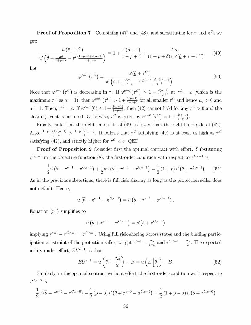
Proof of Proposition 7 Combining (47) and (48), and substituting for τ and πC , we

get:

u′(θ + τC)

u′(θ + ∆θ

1+p−δ − τC1−p+δ+2(ρ−1)

1+p−δ

) = 1 +2 (ρ− 1)

1− p+ δ+

2µ1

(1− p+ δ) cu′(θ + τ − πC)(49)

Let

ϕe=0(τC)≡ u′(θ + τC)

u′(θ + ∆θ

1+p−δ − τC1−p+δ+2(ρ−1)

1+p−δ

) (50)

Note that ϕe=0(τC)is decreasing in τ . If ϕe=0

(τC)> 1 + 2(ρ−1)

1−p+δ at τC = c (which is the

maximum τC as α = 1), then ϕe=0(τC)> 1 + 2(ρ−1)

1−p+δ for all smaller τC and hence µ1 > 0 and

α = 1. Then, τC = c. If ϕe=0 (0) ≤ 1 + 2(ρ−1)1−p+δ , then (42) cannot hold for any τ

C > 0 and the

clearing agent is not used. Otherwise, τC is given by ϕe=0(τC)

= 1 + 2(ρ−1)1−p+δ .

Finally, note that the right-hand side of (49) is lower than the right-hand side of (42).

Also, 1−p+δ+2(ρ−1)1+p−δ > 1−p+2(ρ−1)

1+p. It follows that τC satisfying (49) is at least as high as τC

satisfying (42), and strictly higher for τC < c. QED

Proof of Proposition 9 Consider first the optimal contract with effort. Substituting

πC,e=1 in the objective function (8), the first-order condition with respect to τC,e=1 is

1

2u(θ − πe=1 − πC,e=1

)+

1

2pu(θ + τ e=1 − πC,e=1

)=

1

2(1 + p) u

(θ + τC,e=1

)(51)

As in the previous subsections, there is full risk-sharing as long as the protection seller does

not default. Hence,

u(θ − πe=1 − πC,e=1

)= u

(θ + τ e=1 − πC,e=1

).

Equation (51) simplifies to

u(θ + τ e=1 − πC,e=1

)= u

(θ + τC,e=1

)implying τ e=1−πC,e=1 = τC,e=1. Using full risk-sharing across states and the binding partic-

ipation constraint of the protection seller, we get τ e=1 = ∆θ1+p

and τC,e=1 = ∆θ2. The expected

utility under effort, EU e=1, is thus

EU e=1 = u

(θ +

∆θ

2

)−B = u

(E[θ])−B. (52)

Similarly, in the optimal contract without effort, the first-order condition with respect to

τC,e=0 is

1

2u(θ − πe=0 − πC,e=0

)+

1

2(p− δ) u

(θ + τ e=0 − πC,e=0

)=

1

2(1 + p− δ) u

(θ + τC,e=0

)36

which yields, using full risk-sharing as long as the protection seller does not default, τ e=0 −πC,e=0 = τC,e=0. Using the binding participation constraint of the protection seller, we get

τ e=0 = ∆θ1+p−δ and τ

C,e=0 = ∆θ2. The expected utility without effort, EU e=0, is thus

EU e=0 = u

(θ +

∆θ

2

)= u

(E[θ]). (53)

Comparing expected utility of the protection buyer under effort and without effort, we

have

EU e=1 = u(E[θ])−B < u

(E[θ])

= EU e=0.

QED

Proof of Proposition 10 Let µ denote the Lagrange multiplier on the protection

seller’s participation constraint. First-order conditions with respect to πe=1, τ e=1, τC,e=1,

πe=1, τ e=1, and τC,e=1 yield

u(θ − πe=1 − πC,e=1) = µ (54)

u(θ + τ e=1 − πC,e=1) = µ (55)(12

+ γ)u(θ − πe=1 − πC,e=1)

12

(1 + p) + γ (1− p)+

(12− γ)pu(θ + τ e=1 − πC,e=1)

12

(1 + p) + γ (1− p)= u(θ + τC,e=1) (56)

u(θ − πe=1 − πC,e=1) = µ (57)

u(θ + τ e=1 − πC,e=1) = µ (58)(12− γ)u(θ − πe=1 − πC,e=1)

12

(1 + p)− γ (1− p)+

(12

+ γ)pu(θ + τ e=1 − πC,e=1)

12

(1 + p)− γ (1− p)= u(θ + τC,e=1) (59)

By (54), the participation constraint of the protection seller binds. Using (54) and (55) in

(56), and simplifying yields:

u(θ + τC,e=1) = µ

Similarly, using (57) and (58) in (59), and simplifying yields

u(θ + τC,e=1) = µ

Using full risk-sharing across states, the binding participation constraint of the protection

seller and (20), we get

τC,e=1 = τC,e=1 =∆θ

2

37

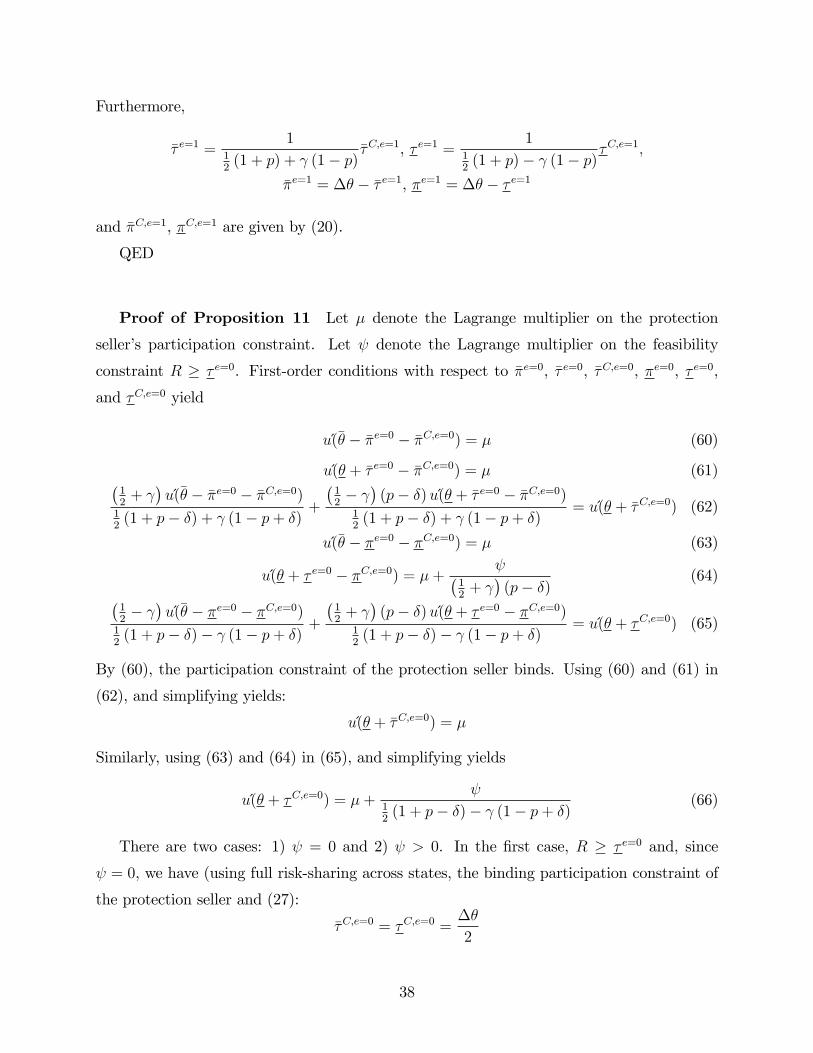
Furthermore,

τ e=1 =1

12

(1 + p) + γ (1− p)τC,e=1, τ e=1 =

112

(1 + p)− γ (1− p)τC,e=1,

πe=1 = ∆θ − τ e=1, πe=1 = ∆θ − τ e=1

and πC,e=1, πC,e=1 are given by (20).

QED

Proof of Proposition 11 Let µ denote the Lagrange multiplier on the protection

seller’s participation constraint. Let ψ denote the Lagrange multiplier on the feasibility

constraint R ≥ τ e=0. First-order conditions with respect to πe=0, τ e=0, τC,e=0, πe=0, τ e=0,

and τC,e=0 yield

u(θ − πe=0 − πC,e=0) = µ (60)

u(θ + τ e=0 − πC,e=0) = µ (61)(12

+ γ)u(θ − πe=0 − πC,e=0)

12

(1 + p− δ) + γ (1− p+ δ)+

(12− γ)

(p− δ) u(θ + τ e=0 − πC,e=0)12

(1 + p− δ) + γ (1− p+ δ)= u(θ + τC,e=0) (62)

u(θ − πe=0 − πC,e=0) = µ (63)

u(θ + τ e=0 − πC,e=0) = µ+ψ(

12

+ γ)

(p− δ)(64)(

12− γ)u(θ − πe=0 − πC,e=0)

12

(1 + p− δ)− γ (1− p+ δ)+

(12

+ γ)

(p− δ) u(θ + τ e=0 − πC,e=0)12

(1 + p− δ)− γ (1− p+ δ)= u(θ + τC,e=0) (65)

By (60), the participation constraint of the protection seller binds. Using (60) and (61) in

(62), and simplifying yields:

u(θ + τC,e=0) = µ

Similarly, using (63) and (64) in (65), and simplifying yields

u(θ + τC,e=0) = µ+ψ

12

(1 + p− δ)− γ (1− p+ δ)(66)

There are two cases: 1) ψ = 0 and 2) ψ > 0. In the first case, R ≥ τ e=0 and, since

ψ = 0, we have (using full risk-sharing across states, the binding participation constraint of

the protection seller and (27):

τC,e=0 = τC,e=0 =∆θ

2

38

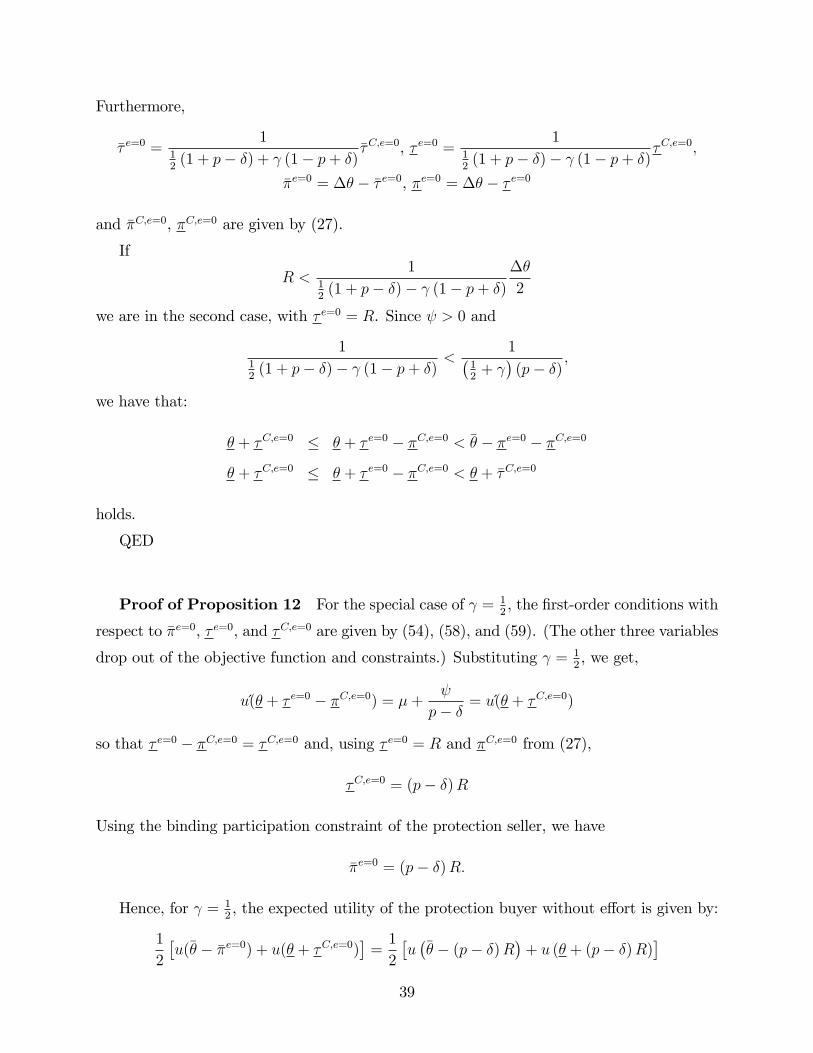
Furthermore,

τ e=0 =1

12

(1 + p− δ) + γ (1− p+ δ)τC,e=0, τ e=0 =

112

(1 + p− δ)− γ (1− p+ δ)τC,e=0,

πe=0 = ∆θ − τ e=0, πe=0 = ∆θ − τ e=0

and πC,e=0, πC,e=0 are given by (27).

If

R <1

12

(1 + p− δ)− γ (1− p+ δ)

∆θ

2

we are in the second case, with τ e=0 = R. Since ψ > 0 and

112

(1 + p− δ)− γ (1− p+ δ)<

1(12

+ γ)

(p− δ),

we have that:

θ + τC,e=0 ≤ θ + τ e=0 − πC,e=0 < θ − πe=0 − πC,e=0

θ + τC,e=0 ≤ θ + τ e=0 − πC,e=0 < θ + τC,e=0

holds.

QED

Proof of Proposition 12 For the special case of γ = 12, the first-order conditions with

respect to πe=0, τ e=0, and τC,e=0 are given by (54), (58), and (59). (The other three variables

drop out of the objective function and constraints.) Substituting γ = 12, we get,

u(θ + τ e=0 − πC,e=0) = µ+ψ

p− δ = u(θ + τC,e=0)

so that τ e=0 − πC,e=0 = τC,e=0 and, using τ e=0 = R and πC,e=0 from (27),

τC,e=0 = (p− δ)R

Using the binding participation constraint of the protection seller, we have

πe=0 = (p− δ)R.

Hence, for γ = 12, the expected utility of the protection buyer without effort is given by:

1

2

[u(θ − πe=0) + u(θ + τC,e=0)

]=

1

2

[u(θ − (p− δ)R

)+ u (θ + (p− δ)R)

]39

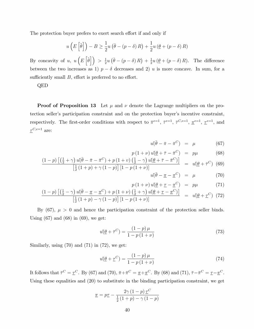
The protection buyer prefers to exert search effort if and only if

u(E[θ])−B ≥ 1

2u(θ − (p− δ)R

)+

1

2u (θ + (p− δ)R)

By concavity of u, u(E[θ])

> 12u(θ − (p− δ)R

)+ 1

2u (θ + (p− δ)R). The difference

between the two increases as 1) p − δ decreases and 2) u is more concave. In sum, for a

suffi ciently small B, effort is preferred to no effort.

QED

Proof of Proposition 13 Let µ and ν denote the Lagrange multipliers on the pro-

tection seller’s participation constraint and on the protection buyer’s incentive constraint,

respectively. The first-order conditions with respect to πe=1, τ e=1, τC,e=1, πe=1, τ e=1, and

τC,e=1 are:

u(θ − π − πC) = µ (67)

p (1 + ν) u(θ + τ − πC) = pµ (68)

(1− p)[(

12

+ γ)u(θ − π − πC) + p (1 + v)

(12− γ)u(θ + τ − πC)

][12

(1 + p) + γ (1− p)]

[1− p (1 + ν)]= u(θ + τC) (69)

u(θ − π − πC) = µ (70)

p (1 + ν) u(θ + τ − πC) = pµ (71)

(1− p)[(

12− γ)u(θ − π − πC) + p (1 + ν)

(12

+ γ)u(θ + τ − πC)

][12

(1 + p)− γ (1− p)]

[1− p (1 + ν)]= u(θ + τC) (72)

By (67), µ > 0 and hence the participation constraint of the protection seller binds.

Using (67) and (68) in (69), we get:

u(θ + τC) =(1− p)µ

1− p (1 + ν)(73)

Similarly, using (70) and (71) in (72), we get:

u(θ + τC) =(1− p)µ

1− p (1 + ν)(74)

It follows that τC = τC . By (67) and (70), π+πC = π+πC . By (68) and (71), τ−πC = τ−πC .Using these equalities and (20) to substitute in the binding participation constraint, we get

π = pτ − 2γ (1− p) τC12

(1 + p)− γ (1− p)

40

which yields π as a function of τ and τC .

Furthermore, it must be that ν > 0 in the optimum so that the incentive constraint binds.

Suppose not, i.e., ν = 0. Then, marginal utilities are equalized across all states, implying

that τ− πC = τC and τ−πC = τC . But then, the incentive constraint cannot hold as B > 0.

A contradiction. Since the incentive constraint binds, we have, using τ − πC = τ − πC andτC = τC ,

u(θ + τ − πC)− u(θ + τC) =2B

δ

This equation yields τ as a function of τC .

Next, note that by (70) and (71),

u(θ − π − πC)

u(θ + τ − πC)= 1 + ν > 1

since ν > 0. It follows that θ + τ − πC > θ − π − πC . Furthermore, by (74), we have

u(θ + τC) =(1− p)

1− p (1 + ν)u(θ − π − πC)

Since 1 + ν > 1, we have that θ − π − πC > θ + τC . The optimal transfer τC is given by:

u(θ + τC) =(1− p) u(θ − π − πC)u(θ + τ − πC)

u(θ + τ − πC)− pu(θ − π − πC)

In sum, protection buyer’s utilities are no longer equalized, even when the protection

seller does not default, and

θ + τ − πC = θ + τ − πC > θ − π − πC = θ − π − πC > θ + τC = θ + τC

holds in the optimum. QED

Proof of Proposition 15 For γ = 12, the expected utility under no effort is given by

1

2u(θ − (p− δ)R

)+

1

2u (θ + (p− δ)R)

Since the incentive-compatibility constraint binds in the optimal contract with effort, i.e.,

u(θ + τ − πC)− u(θ + τC) =2B

δ,

41

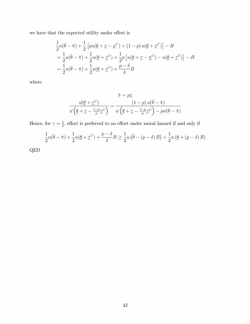
we have that the expected utility under effort is

1

2u(θ − π) +

1

2

[pu(θ + τ − πC) + (1− p)u(θ + τC)

]−B

=1

2u(θ − π) +

1

2u(θ + τC) +

1

2p[u(θ + τ − πC)− u(θ + τC)

]−B

=1

2u(θ − π) +

1

2u(θ + τC) +

p− δδ

B

where

π = pτ

u(θ + τC)

u(θ + τ − 1−p

pτC) =

(1− p) u(θ − π)

u(θ + τ − 1−p

pτC)− pu(θ − π)

Hence, for γ = 12, effort is preferred to no effort under moral hazard if and only if

1

2u(θ − π) +

1

2u(θ + τC) +

p− δδ

B ≥ 1

2u(θ − (p− δ)R

)+

1

2u (θ + (p− δ)R)

QED

42