Figure 5. Testing spotted owl model with sites of known occurrence and random sites. CLAMS Wildlife Habitat Capability Index Models Coastal Landscape Analysis and Modeling Study; College of Forestry, Oregon State University, USDA Forest Service, Pacific Northwest Research Station, Corvallis, OR; Oregon Department of Forestry William C. McComb, Department of Natural Resources Conservation, University of Massachusetts, Amherst, MA Michael T. McGrath, Montana Department of Natural Resources and Conservation, Missoula, MT Thomas A. Spies, USDA Forest Service Pacific Northwest Research Station, Corvallis, OR June 2002 Introduction Forest management policies in the Pacific Northwest and the southeastern United States have previously been criticized for failing to maintain threatened species habitat or to provide habitat for early successional species. Thus, long-term forest policy planning requires the management of biodiversity on the landscape scale with coarse filters and fine filters. Coarse filters involve monitoring a variety of species through use of broad habitat requirements and assume that specific habitat requirements will be provided. The fine filter approach is designed to “catch” rare and noteworthy species that might otherwise slip through the coarse filter. CLAMS fine filter models do so by estimating habitat capability for 17 species through the use of multi-scale habitat relationship information from data sets, published research, and expert opinion. Objectives We developed a habitat modeling approach to evaluate forest management policies. Our approach has the following characteristics: 1. Quantify the current capability of sites across the Oregon Coast Range to provide habitat for focal species. 2. Provide spatially-explicit estimates of habitat capability for focal species for possible future landscapes. 3. Estimate the effects of alternative forest management actions, including silvicultural treatments, on habitat at stand and landscape scales. Methods The key to selecting species for the fine filter is to select focal species whose status and time trend provide insights into the integrity of the larger ecological sys tem. This is accomplished by selecting species in categories that reflect ecological integrity and also societal concerns. This focal species approach differs from the more widely known indicator species concept because it examines species based on properties that are likely to be overlooked by the coarse filter (e.g., narrow endemism, ecological engineer, large home range, etc.), rather than species that might represent habitat needs of several species. We developed a set of criteria and focal species that reflect characteristics of ecological integrity as well as societal concerns (e.g., listed and game species; Table 1). For each focal species we developed habitat-relationship models to characterize species occurrences and potential quality of habitat. Because habitat is species-specific, we assumed that no pre-defined vegetation classes could describe habitat suitability for all species. Thus, we developed a habitat suitability modeling approach based on the specific habitat elements as determined from the state of knowledge of the biology of the species. We took a spatially explicit approach to modeling habitat for each of the focal species. In general, species’ habitat requirements were modeled from single pixels up to areas representing their home range (Fig. 1—pixel and circles). For species that operate from a central place (e.g., nest or den site), each 25- x 25-m pixel is evaluated relative to its potential to provide a nest or den site during the breeding season, based on the estimates of fine-scale features within the focal pixel and conditions surrounding it (a 9-pixel window of 0.56 ha surrounding the focal pixel). In addition, landscape scales relative to the species’ home range and other biologically relevant scales surrounding the focal pixel are evaluated for their ability to provide other life history requirements (Fig. 1). Modeling Process Determination of which variables to include in the model, their relationships, and the response of habitat capability to each variable begins with a literature review for the species (Fig. 2). Potential variables are evaluated based on four criteria: 1. There is an empirical relationship between reproduction or survival with the variable. 2. The variables can be estimated from existing GIS layers, including vegetation data. 3. The variable can be projected into the future using models of forest dynamics. 4. The variable has a noticeable influence on habitat capability for the species. 0 0.1 0.2 0.3 0.4 0.5 0.6 0.7 0.8 0.9 1 0 50 100 150 200 250 300 350 400 450 Trees per Hectare 10 < DBH le 25 cm Capability Index 0 0.1 0.2 0.3 0.4 0.5 0.6 0.7 0.8 0.9 1 0 25 50 75 100 125 150 175 200 225 Trees per Hectare 25 < DBH le 50 cm Capability Index 0 0.1 0.2 0.3 0.4 0.5 0.6 0.7 0.8 0.9 1 0 10 20 30 40 50 60 70 80 90 Trees per Hectare DBH > 75 cm Capability Index Model 3 Original Model 4 0 0.1 0.2 0.3 0.4 0.5 0.6 0.7 0.8 0.9 1 0 1 2 3 4 5 6 7 8 9 10 Diameter Diversity Index Capability Index 0 0.1 0.2 0.3 0.4 0.5 0.6 0.7 0.8 0.9 1 0 0.1 0.2 0.3 0.4 0.5 0.6 0.7 0.8 0.9 1 Proportion in Large Tree Habitat Capability Index Original Model 2 0 0.1 0.2 0.3 0.4 0.5 0.6 0.7 0.8 0.9 1 0 10 20 30 40 50 60 70 80 90 100 110 Trees per Hectare Capability Index Original Model 5 Model 6 Table 2 . Alternative northern spotted owl model hypotheses. Model Hypothesis M 0 Original model hypothesis. M 1 The surrounding landscape is not related to habitat capability for spotted owls (i.e., no landscape effect). M 2 Habitat capability increases more rapidly with increasing area of large-tree stands within 0.3 km of spotted owl nests than in the original model. M 3 Habitat capability increases more rapidly with more trees dbh > 75 cm. M 4 Habitat capability increases more slowly with more trees dbh > 75 cm. M 5 Potential nest trees are represented by the density of trees dbh > 50 cm. M 6 Potential nest trees are represented by the density of trees dbh > 100 cm. Equations for spotted owl model: where HSI = habitat suitability index f = the focal pixel NSI = nesting suitability index (Eq. 2) LSI = landscape suitability index (Eq. 7) where NSI = Nesting Suitability Index f = focal pixel i = pixel D1 = Index for the density of trees 10 < dbh # 25 cm D2 = Index for the density of trees 25 < dbh # 50 cm D3 = Index for the density of trees dbh > 75 cm D4 = diameter diversity index where LSI f = landscape suitability index for the focal pixel S 1 = habitat index for 0.3-km radius surrounding the focal pixel S 2 = habitat index for 0.8-km radius surrounding the focal pixel S 3 = home range index, representing a 2.4-km radius surrounding the focal pixel HSI NSI LSI f f f = 2 3 * NSI D D D D f i = = ∑ 1 2 3 4 4 9 2 1 9 LSI S S S f = 1 3 2 2 3 6 * * Figure 4. Watersheds from which sensitivity analysis data are derived. Figure 6 . Spotted owl Habitat Capability map for current vegetative conditions. Figure 1. After the “best” model has been identified, it is then implemented to identify habitat capable for the species on a map of current vegetation (Fig. 6—owl hci map). This map is then linked with a vegetation dynamics model and we are able to evaluate future patterns of habitat capability. Where uncertainty exists in habitat-relationships, several different models can be estimated to show the range of uncertainty. Figure 2 Once the revised model and sensitivity analyses are completed, alternative models are developed, based on reviewer comments or competing hypotheses in the literature, to test individual variable response functions and the necessity of sub-indices (Table 2—list of owl hypotheses). This is accomplished through using field data with known locations and absences (Fig. 5—owl locations), and testing via an information-theoretic approach in logistic regression, with the HCI score as the explanatory variable. The hypothesis with the lowest AIC score is then identified as the “best” model hypothesis (Table 3—AIC results). Table 3. Validation regression and classification accuracy results for the original and six alternative northern spotted owl HCI models. Model ♠AIC HCI Breakpoint Classification Accuracy (%) Type II error (%) 1 M 2 0.0 0.37 75.5 10.0 M 5 4.75 0.28 75.5 11.6 M 6 8.12 0.29 75.8 12.3 M 4 8.26 0.28 75.8 11.9 M 0 8.56 0.29 75.5 12.4 M 3 10.27 0.24 76.1 8.4 M 1 11.56 0.33 72.6 13.6 1 The number of known spotted owl nests sites misclassified as unused sites, at the reported HCI breakpoint, divided by the total number of known spotted owl nest sites ( n = 155) and multiplied by 100. Examples of variables selected for the spotted owl HCI model, and their relationships, are outlined in Figure 3 (owl response function graphs and equations). The sensitivity analysis is conducted to ensure the range of variability for each variable is represented; this analysis is done for three watersheds in the Coast Range: Nehalem, Alsea, and Umpqua, to allow evaluation of northern, central, and southern watersheds, respectively (Fig. 4). This analysis is conducted with 1,000 Monte Carlo iterations using the Latin hypercube sampling method applied to the probability distribution of each variable. Correlation between HCI score and explanatory variable variation are then evaluated. X X X X X X X X X X Risk X Tailed Frog Torrent Salamander X X Beaver Dams X X X Elk X Fisher X Marten X Long-legged Bat X X Red-tree Vole X X Mountain Beaver X X X Northern Goshawk X Black-throated Gray Warbler X Western Bluebird X Olive-sided Flycatcher X Downy Woodpecker X X Pileated Woodpecker X X Marbled Murrelet X X X Northern Spotted Owl Public/Regulatory Interest Game Species Link Species Umbrella Species Ecological Function Seral Stage Association SPECIES Focal Species Criteria Table 1. Focal species selected for fine filter modeling and the criteria for which they were selected. Figure 3 . Graphs and equations of spotted owl response functions. 1996

Welcome message from author
This document is posted to help you gain knowledge. Please leave a comment to let me know what you think about it! Share it to your friends and learn new things together.
Transcript
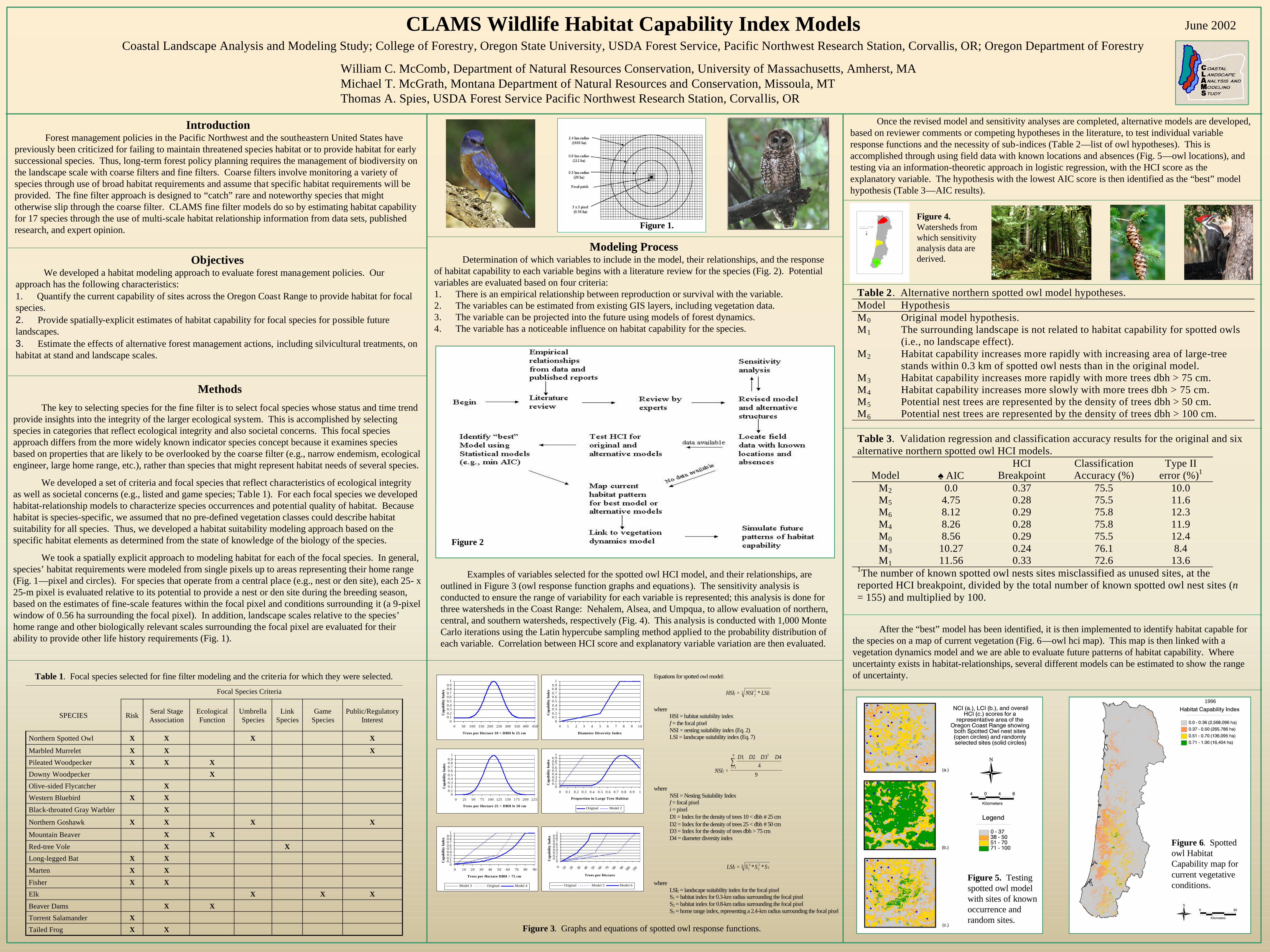
Figure 5. Testing spotted owl model with sites of known occurrence and random sites.
CLAMS Wildlife Habitat Capability Index ModelsCoastal Landscape Analysis and Modeling Study; College of Forestry, Oregon State University, USDA Forest Service, Pacific Northwest Research Station, Corvallis, OR; Oregon Department of Forestry
William C. McComb, Department of Natural Resources Conservation, University of Massachusetts, Amherst, MA Michael T. McGrath, Montana Department of Natural Resources and Conservation, Missoula, MTThomas A. Spies, USDA Forest Service Pacific Northwest Research Station, Corvallis, OR
June 2002
IntroductionForest management policies in the Pacific Northwest and the southeastern United States have
previously been criticized for failing to maintain threatened species habitat or to provide habitat for early successional species. Thus, long-term forest policy planning requires the management of biodiversity on the landscape scale with coarse filters and fine filters. Coarse filters involve monitoring a variety of species through use of broad habitat requirements and assume that specific habitat requirements will be provided. The fine filter approach is designed to “catch” rare and noteworthy species that might otherwise slip through the coarse filter. CLAMS fine filter models do so by estimating habitat capability for 17 species through the use of multi-scale habitat relationship information from data sets, publishedresearch, and expert opinion.
ObjectivesWe developed a habitat modeling approach to evaluate forest management policies. Our
approach has the following characteristics:1. Quantify the current capability of sites across the Oregon Coast Range to provide habitat for focal species.2. Provide spatially-explicit estimates of habitat capability for focal species for possible future landscapes.3. Estimate the effects of alternative forest management actions, including silvicultural treatments, on habitat at stand and landscape scales.
Methods
The key to selecting species for the fine filter is to select focal species whose status and time trend provide insights into the integrity of the larger ecological system. This is accomplished by selecting species in categories that reflect ecological integrity and also societal concerns. This focal species approach differs from the more widely known indicator species concept because it examines species based on properties that are likely to be overlooked by the coarse filter (e.g., narrow endemism, ecological engineer, large home range, etc.), rather than species that might represent habitat needs of several species.
We developed a set of criteria and focal species that reflect characteristics of ecological integrity as well as societal concerns (e.g., listed and game species; Table 1). For each focal species we developed habitat-relationship models to characterize species occurrences and potential quality of habitat. Because habitat is species-specific, we assumed that no pre-defined vegetation classes could describe habitat suitability for all species. Thus, we developed a habitat suitability modeling approach based on the specific habitat elements as determined from the state of knowledge of the biology of the species.
We took a spatially explicit approach to modeling habitat for each of the focal species. In general, species’ habitat requirements were modeled from single pixels up to areas representing their home range (Fig. 1—pixel and circles). For species that operate from a central place (e.g., nest or den site), each 25- x 25-m pixel is evaluated relative to its potential to provide a nest or den site during the breeding season, based on the estimates of fine-scale features within the focal pixel and conditions surrounding it (a 9-pixel window of 0.56 ha surrounding the focal pixel). In addition, landscape scales relative to the species’home range and other biologically relevant scales surrounding the focal pixel are evaluated for their ability to provide other life history requirements (Fig. 1).
Modeling ProcessDetermination of which variables to include in the model, their relationships, and the response
of habitat capability to each variable begins with a literature review for the species (Fig. 2). Potential variables are evaluated based on four criteria:1. There is an empirical relationship between reproduction or survival with the variable.2. The variables can be estimated from existing GIS layers, including vegetation data.3. The variable can be projected into the future using models of forest dynamics.4. The variable has a noticeable influence on habitat capability for the species.
00.10.20.30.40.50.60.70.80.9
1
0 50 100 150 200 250 300 350 400 450
Trees per Hectare 10 < DBH le 25 cm
Cap
abili
ty I
ndex
00.10.20.30.40.50.60.70.80.9
1
0 25 50 75 100 125 150 175 200 225
Trees per Hectare 25 < DBH le 50 cm
Cap
abili
ty I
ndex
00.10.20.30.40.50.60.70.80.9
1
0 10 20 30 40 50 60 70 80 90
Trees per Hectare DBH > 75 cm
Cap
abili
ty I
ndex
Model 3 Original Model 4
00.10.20.30.40.50.60.70.80.9
1
0 1 2 3 4 5 6 7 8 9 10
Diameter Diversity Index
Cap
abili
ty I
ndex
00.10.20.30.40.50.60.70.80.9
1
0 0.1 0.2 0.3 0.4 0.5 0.6 0.7 0.8 0.9 1
Proportion in Large Tree Habitat
Cap
abili
ty I
ndex
Original Model 2
00.10.20.30.40.50.60.70.80.9
1
0 10 20 30 40 50 60 70 80 90 100 110
Trees per Hectare
Cap
abili
ty I
ndex
Original Model 5 Model 6
Table 2. Alternative northern spotted owl model hypotheses. Model Hypothesis M0 Original model hypothesis. M1 The surrounding landscape is not related to habitat capability for spotted owls
(i.e., no landscape effect). M2 Habitat capability increases more rapidly with increasing area of large-tree
stands within 0.3 km of spotted owl nests than in the original model. M3 Habitat capability increases more rapidly with more trees dbh > 75 cm. M4 Habitat capability increases more slowly with more trees dbh > 75 cm. M5 Potential nest trees are represented by the density of trees dbh > 50 cm. M6 Potential nest trees are represented by the density of trees dbh > 100 cm.
Equations for spotted owl model:
where HSI = habitat suitability index f = the focal pixel NSI = nesting suitability index (Eq. 2) LSI = landscape suitability index (Eq. 7)
where NSI = Nesting Suitability Index f = focal pixel i = pixel D1 = Index for the density of trees 10 < dbh # 25 cm D2 = Index for the density of trees 25 < dbh # 50 cm D3 = Index for the density of trees dbh > 75 cm D4 = diameter diversity index
where LSIf = landscape suitability index for the focal pixel S1 = habitat index for 0.3-km radius surrounding the focal pixel S2 = habitat index for 0.8-km radius surrounding the focal pixel S3 = home range index, representing a 2.4-km radius surrounding the focal pixel
HSI NSI LSIf f f= 23 *
NSI
D D D D
fi
=
+ + +
=∑ 1 2 3 4
4
9
2
1
9
LSI S S Sf = 13
22
36 * *
Figure 4.Watersheds from which sensitivity analysis data are derived.
Figure 6. Spotted owl Habitat Capability map for current vegetative conditions.
Figure 1.
After the “best” model has been identified, it is then implemented to identify habitat capable for the species on a map of current vegetation (Fig. 6—owl hci map). This map is then linked with a vegetation dynamics model and we are able to evaluate future patterns of habitat capability. Where uncertainty exists in habitat-relationships, several different models can be estimated to show the range of uncertainty.
Figure 2
Once the revised model and sensitivity analyses are completed, alternative models are developed, based on reviewer comments or competing hypotheses in the literature, to test individual variable response functions and the necessity of sub-indices (Table 2—list of owl hypotheses). This is accomplished through using field data with known locations and absences (Fig. 5—owl locations), and testing via an information-theoretic approach in logistic regression, with the HCI score as the explanatory variable. The hypothesis with the lowest AIC score is then identified as the “best” model hypothesis (Table 3—AIC results).
Table 3. Validation regression and classification accuracy results for the original and six alternative northern spotted owl HCI models.
Model ♠AIC HCI
Breakpoint Classification Accuracy (%)
Type II error (%)1
M2 0.0 0.37 75.5 10.0 M5 4.75 0.28 75.5 11.6 M6 8.12 0.29 75.8 12.3 M4 8.26 0.28 75.8 11.9 M0 8.56 0.29 75.5 12.4 M3 10.27 0.24 76.1 8.4 M1 11.56 0.33 72.6 13.6
1The number of known spotted owl nests sites misclassified as unused sites, at the reported HCI breakpoint, divided by the total number of known spotted owl nest sites (n = 155) and multiplied by 100.
Examples of variables selected for the spotted owl HCI model, and their relationships, are outlined in Figure 3 (owl response function graphs and equations). The sensitivity analysis is conducted to ensure the range of variability for each variable is represented; this analysis is done for three watersheds in the Coast Range: Nehalem, Alsea, and Umpqua, to allow evaluation of northern, central, and southern watersheds, respectively (Fig. 4). This analysis is conducted with 1,000 Monte Carlo iterations using the Latin hypercube sampling method applied to the probability distribution of each variable. Correlation between HCI score and explanatory variable variation are then evaluated.
X
X
X
X
X
X
X
X
X
X
Risk
XTailed Frog
Torrent Salamander
XXBeaver Dams
XXXElk
XFisher
XMarten
XLong-legged Bat
XXRed-tree Vole
XXMountain Beaver
XXXNorthern Goshawk
XBlack-throated Gray Warbler
XWestern Bluebird
XOlive-sided Flycatcher
XDowny Woodpecker
XXPileated Woodpecker
XXMarbled Murrelet
XXXNorthern Spotted Owl
Public/Regulatory Interest
Game Species
Link Species
Umbrella Species
Ecological Function
Seral Stage Association
SPECIES
Focal Species Criteria
Table 1. Focal species selected for fine filter modeling and the criteria for which they were selected.
Figure 3. Graphs and equations of spotted owl response functions.
1996
Related Documents