19970 Phys. Chem. Chem. Phys., 2011, 13, 19970–19978 This journal is c the Owner Societies 2011 Cite this: Phys. Chem. Chem. Phys., 2011, 13, 19970–19978 Water under temperature gradients: polarization effects and microscopic mechanisms of heat transfer Jordan Muscatello, a Frank Ro¨mer, a Jona´s Sala ab and Fernando Bresme* a Received 10th June 2011, Accepted 27th September 2011 DOI: 10.1039/c1cp21895f We report non-equilibrium molecular dynamics simulations (NEMD) of water under temperature gradients using a modified version of the central force model (MCFM). This model is very accurate in predicting the equation of state of water for a wide range of pressures and temperatures. We investigate the polarization response of water to thermal gradients, an effect that has been recently predicted using Non-Equilibrium Thermodynamics (NET) theory and computer simulations, as a function of the thermal gradient strength. We find that the polarization of the liquid varies linearly with the gradient strength, which indicates that the ratio of phenomenological coefficients regulating the coupling between the polarization response and the heat flux is independent of the gradient strength investigated. This notion supports the NET theoretical predictions. The coupling effect leading to the liquid polarization is fairly strong, leading to polarization fields of B10 3–6 Vm 1 for gradients of B10 5–8 Km 1 , hence confirming earlier estimates. Finally we employ our NEMD approach to investigate the microscopic mechanism of heat transfer in water. The image emerging from the computation and analysis of the internal energy fluxes is that the transfer of energy is dominated by intermolecular interactions. For the MCFM model, we find that the contribution from hydrogen and oxygen is different, with the hydrogen contribution being larger than that of oxygen. 1 Introduction Temperature gradients can result in strong coupling effects. 1,2 It is well known that particles in aqueous solutions move as a response to an imposed temperature gradient. 3,4 This is the so called Soret effect, also known as thermophoresis. 1 This effect is also observed in binary mixtures 5 and it has been used to separate isotopic mixtures. The thermoelectric response, namely charge transport induced by a temperature gradient, is the basis of a wide range of thermoelectric devices, which can convert waste heat into electricity. 6 An analog of this thermoelectric phenomenon is also observed in aqueous solu- tions. Here the charge carriers are ions. The temperature gradients lead to salinity gradients, which can in turn modify the thermophoretic response of large colloidal particles. 7 It has been recently discussed that similar thermoelectric phenomena are exploited by sharks to sense temperature gradients. 8 The thermoelectric material in this case is a gel, containing salt and water. This thermoelectric mechanism would provide sharks with a natural device to detect temperature changes in the surroundings without the intervention of ion channels. The relevance of water as a medium to enable many of the non-equilibrium phenomena discussed above is obvious. However it is not so obvious how a complex liquid such as water behaves under the non-equilibrium conditions imposed by thermal gradients, and how heat is transferred through the liquid. Our microscopic understanding of the non-equilibrium response of water is still poor. Most works to date have been devoted to equilibrium studies. A significant number of these equilibrium investigations have been performed using computer simulations. These studies show that relatively simple models can explain the enormous complexity of the phase diagram of water and ice from a truly microscopic perspective. 9 These models have also helped to uncover new physical phenomena at low temperatures, 10,11 and to understand the complex interfacial behavior of water, 12–17 which is so relevant to explain the role that water plays in tuning the interactions between hydrophobic and hydrophilic surfaces. We have recently explored the behavior of water under thermal gradients. 18 Using non-equilibrium molecular dynamics simulations of the Central Force Model of water, 19,20 we found that the water molecules tend to adopt a preferred orientation, with the dipole aligning with the gradient and the hydrogen atoms pointing preferentially towards the cold region, a Chemical Physics Section, Department of Chemistry, Imperial College London, The Thomas Young Centre and London Centre for Nanotechnology, SW7 2AZ, London, UK. E-mail: [email protected] b Departament de Fsica i Enginyeria Nuclear, Universitat Politcnica de Catalunya, B4-B5 Campus Nord, 08034 Barcelona, Spain PCCP Dynamic Article Links www.rsc.org/pccp PAPER Downloaded by Massachusetts Institute of Technology on 06 February 2012 Published on 11 October 2011 on http://pubs.rsc.org | doi:10.1039/C1CP21895F View Online / Journal Homepage / Table of Contents for this issue

Welcome message from author
This document is posted to help you gain knowledge. Please leave a comment to let me know what you think about it! Share it to your friends and learn new things together.
Transcript
19970 Phys. Chem. Chem. Phys., 2011, 13, 19970–19978 This journal is c the Owner Societies 2011
Cite this: Phys. Chem. Chem. Phys., 2011, 13, 19970–19978
Water under temperature gradients: polarization effects and microscopic
mechanisms of heat transfer
Jordan Muscatello,aFrank Romer,
aJonas Sala
aband Fernando Bresme*
a
Received 10th June 2011, Accepted 27th September 2011
DOI: 10.1039/c1cp21895f
We report non-equilibrium molecular dynamics simulations (NEMD) of water under temperature
gradients using a modified version of the central force model (MCFM). This model is very
accurate in predicting the equation of state of water for a wide range of pressures and
temperatures. We investigate the polarization response of water to thermal gradients, an effect
that has been recently predicted using Non-Equilibrium Thermodynamics (NET) theory and
computer simulations, as a function of the thermal gradient strength. We find that the
polarization of the liquid varies linearly with the gradient strength, which indicates that the ratio
of phenomenological coefficients regulating the coupling between the polarization response and
the heat flux is independent of the gradient strength investigated. This notion supports the NET
theoretical predictions. The coupling effect leading to the liquid polarization is fairly strong,
leading to polarization fields of B103–6 V m�1 for gradients of B105–8 K m�1, hence confirming
earlier estimates. Finally we employ our NEMD approach to investigate the microscopic
mechanism of heat transfer in water. The image emerging from the computation and analysis of
the internal energy fluxes is that the transfer of energy is dominated by intermolecular
interactions. For the MCFM model, we find that the contribution from hydrogen and oxygen is
different, with the hydrogen contribution being larger than that of oxygen.
1 Introduction
Temperature gradients can result in strong coupling effects.1,2
It is well known that particles in aqueous solutions move as a
response to an imposed temperature gradient.3,4 This is the so
called Soret effect, also known as thermophoresis.1 This effect
is also observed in binary mixtures5 and it has been used to
separate isotopic mixtures. The thermoelectric response,
namely charge transport induced by a temperature gradient,
is the basis of a wide range of thermoelectric devices, which
can convert waste heat into electricity.6 An analog of this
thermoelectric phenomenon is also observed in aqueous solu-
tions. Here the charge carriers are ions. The temperature
gradients lead to salinity gradients, which can in turn modify
the thermophoretic response of large colloidal particles.7 It has
been recently discussed that similar thermoelectric phenomena
are exploited by sharks to sense temperature gradients.8 The
thermoelectric material in this case is a gel, containing salt and
water. This thermoelectric mechanism would provide sharks
with a natural device to detect temperature changes in the
surroundings without the intervention of ion channels.
The relevance of water as a medium to enable many of the
non-equilibrium phenomena discussed above is obvious.
However it is not so obvious how a complex liquid such as
water behaves under the non-equilibrium conditions imposed
by thermal gradients, and how heat is transferred through the
liquid. Our microscopic understanding of the non-equilibrium
response of water is still poor. Most works to date have been
devoted to equilibrium studies. A significant number of these
equilibrium investigations have been performed using
computer simulations. These studies show that relatively
simple models can explain the enormous complexity of the
phase diagram of water and ice from a truly microscopic
perspective.9 These models have also helped to uncover new
physical phenomena at low temperatures,10,11 and to
understand the complex interfacial behavior of water,12–17
which is so relevant to explain the role that water plays in
tuning the interactions between hydrophobic and hydrophilic
surfaces.
We have recently explored the behavior of water
under thermal gradients.18 Using non-equilibrium molecular
dynamics simulations of the Central Force Model of water,19,20
we found that the water molecules tend to adopt a preferred
orientation, with the dipole aligning with the gradient and the
hydrogen atoms pointing preferentially towards the cold region,
a Chemical Physics Section, Department of Chemistry,Imperial College London, The Thomas Young Centre and LondonCentre for Nanotechnology, SW7 2AZ, London, UK.E-mail: [email protected]
bDepartament de Fsica i Enginyeria Nuclear, Universitat Politcnicade Catalunya, B4-B5 Campus Nord, 08034 Barcelona, Spain
PCCP Dynamic Article Links
www.rsc.org/pccp PAPER
Dow
nloa
ded
by M
assa
chus
etts
Ins
titut
e of
Tec
hnol
ogy
on 0
6 Fe
brua
ry 2
012
Publ
ishe
d on
11
Oct
ober
201
1 on
http
://pu
bs.r
sc.o
rg |
doi:1
0.10
39/C
1CP2
1895
FView Online / Journal Homepage / Table of Contents for this issue
This journal is c the Owner Societies 2011 Phys. Chem. Chem. Phys., 2011, 13, 19970–19978 19971
i.e., the temperature gradient polarizes the liquid. To the best of
our knowledge this represents the first observation of such effect
in a liquid, i.e., an isotropic medium. We note that Lehmann
reported shortly after the discovery of liquid crystals that
temperature gradients can induce uniform
rotation in liquid crystals, i.e., in an anisotropic material.21
Temperature induced polarization effects in liquid crystals have
also been discussed more recently.22
Our initial investigations of water polarization under
thermal gradients indicated that large gradients can induce a
significant polarization, equivalent to an electrostatic field
ofB105 Vm�1 for a gradient ofB107 Km�1. These temperature
gradients are huge for macroscopic standards. However,
gradients of this magnitude are easily achievable at micron
and nanoscales. As a matter of fact gradients of the order of
106 K m�1, 1 K mm�1 can be routinely obtained in experiments
where colloidal particles are heated with lasers.4 Despite these
large gradients, recent experiments on colloidal suspensions3
suggest, and theoretical analysis argues,23 that the behavior of
these suspensions under thermal gradients can be described
using local thermodynamic equilibrium. This idea has been
tested before using computer simulations, where much larger
gradients are achievable. Analysis of the equation of state of
fluids and liquids from these simulations, a notion that we
exploit in this paper, did not reveal significant deviations from
the equation of state obtained at equilibrium.24,25
In this paper we extend our investigations of water under
temperature gradients to (1) investigate the influence of
the temperature gradient strength on the water polarization,
(2) test whether this dependence is consistent with the predictions
of Non-Equilibrium Thermodynamics theory and (3) analyze the
heat transport mechanism in liquid water by computing the
oxygen and hydrogen contributions to the energy flux.
The article is structured as follows. Firstly, we set the
problem from the perspective of the theory of Non-Equilibrium
Thermodynamics. The methodological details, simulation
method and force-field follow. We then present and discuss
our results on the behavior of water under thermal gradients.
A final section containing the main conclusions and final
remarks closes the paper.
2 Non-equilibrium thermodynamics
We are interested in the investigation of the non-equilibrium
response of an isotropic polar fluid to a temperature gradient.
The phenomenological equations defining coupling effects
between polarization and temperature gradients can be
derived using Non-Equilibrium Thermodynamics theory.1,18,26
The polarization induced by the temperature gradient is
described in terms of two linear flux–force relations,
@P
@t¼ �Lpp
TðEeq � EÞ � Lpq
T2rT ð1Þ
Jq ¼ �Lqp
TðEeq � EÞ � Lqq
T2rT ð2Þ
where P is the polarization, Eeq is the equilibrium electrostatic
field, E is the electrostatic field in the sample, Jq is the heat flux
and Lab are the phenomenological coefficients. One equation
that defines the dependence of the electrostatic field E with the
temperature gradient rT has been derived in ref. 18,
E ¼ 1� 1
er
� �Lpq
Lpp
rTT; ð3Þ
which defines the electrostatic field in terms of the dielectric
constant of the liquid er. Eqn (3) shows that the polarization of
the sample (P = �e0E) will reach a maximum value when
er - N. However, the functional form of eqn (3) shows that
the polarization varies rapidly with er, and for high polar liquids
such as water (er = 78 at 298 K) it should be close to the
maximum value for given rT, T and the Lpq/Lpp ratio.
In this paper we will perform a systematic test of eqn (3) by
simulating water at different temperature gradients.
3 Methodology
3.1 Modified central force model
In all the simulations the Modified Central Force Model
(MCFM) of water was used.20,27 This is a flexible three site
model with partial charges on the hydrogens and oxygens
calculated to reproduce the correct dipole moment of water in
the gas phase. The intermolecular interactions in the MCFM
follow the functional form introduced by Lemberg and
Stillinger,19 and the intramolecular interactions are modelled
using harmonic potentials as introduced in ref. 20 and 27.
Other implementations of this model have been proposed.
Guillot and Guissani used a closely related model as a
reference to include quantum effects through the Feynman–
Hibbs formalism.28
The MCFM potential is characterised by the sum of intra-
molecular and intermolecular contributions Uintra,a,b(r) and
Uinter,a,b(r) mediated by a switching function t(r), such that,
Uab(r) = Uintra,ab(r)[1 � tab(r)] + Uinter,ab(r)tab(r) (4)
where tab is given by
tab ¼1
21þ tanh
r� Rab
wab
� �� �ð5Þ
where Rab and wab define the location and the transition from
the intra to the intermolecular potential. Following ref. 20 we
use, ROH = 1.45 A, RHH = 1.88 A, wOH = 0.02 A and wHH =
0.02 A. The oxygen–oxygen, oxygen–hydrogen and hydrogen–
hydrogen intermolecular contributions are given by:
Uinter;OOðrÞ ¼23700
r8:8591� 0:25 exp½�4ðr� 3:4Þ2�
� 0:20 exp½�1:5ðr� 4:5Þ2� þ Z2Oe
2
4pe0r
ð6Þ
Uinter;OHðrÞ ¼�4
1þ exp½5:49305ðr� 2:2Þ� þZOZHe
2
4pe0rð7Þ
Uinter;HHðrÞ ¼Z2
He2
4pe0rð8Þ
with ZH = 0.32983e and ZO = �2ZH. The energies for all the
potential functions are given in kcal mol�1 and distances in A.
Dow
nloa
ded
by M
assa
chus
etts
Ins
titut
e of
Tec
hnol
ogy
on 0
6 Fe
brua
ry 2
012
Publ
ishe
d on
11
Oct
ober
201
1 on
http
://pu
bs.r
sc.o
rg |
doi:1
0.10
39/C
1CP2
1895
F
View Online
19972 Phys. Chem. Chem. Phys., 2011, 13, 19970–19978 This journal is c the Owner Societies 2011
The intramolecular contributions are given by,
Uintra;ab ¼1
2ke;abðr� re;abÞ2 þ
ZaZb
4pe0rð9Þ
where the equilibrium distance, re, and the force constant keare defined by,
re;ab ¼ rb;ab �ZaZbe
2
4pe0kb;abr2b;abð10Þ
ke;ab ¼ kb;ab �2ZaZb
4pe0r3b;abð11Þ
with rb,OH = 0.9584 A, rb,HH = 1.5151 A, kb,OH =
1147.6 kcal (mol A2)�1 and kb,OH = 257.3 kcal (mol A2)�1.
The bond lengths, re, and the force constants, ke, are adjusted
in this way to reproduce the geometry of the water molecule in
the vapour phase.20,27
3.2 Computational details
Non-equilibrium molecular dynamics simulations were performed
using a rectangular box with dimensions {Lx,Ly,Lz} = {5,1,1} �Lz, where Lz = 19.725 A, containing 1280 water molecules.
The cell was divided into 120 layers along the x-axis to enable
the evaluation of local system properties. The Wolf method
was employed to compute the electrostatic interactions.29,30 As
we will see below this method offers a good trade off between
computational efficiency and accuracy in the computation
of bulk properties. The computations were performed with a
cut-off of 9.8 A and a convergence parameter of aLx = 5.6.
In order to set up a thermal gradient in the system, the heat
exchange algorithm (HEX) was used.31 In this method, the
ends and middle layers of the system cell act as heat sources/
sinks, by periodically thermostatting the particles contained in
the layers and thus setting up a heat flux �JU in the system. By
symmetry the fluxes in the two halves of the system cell have
opposite direction, rendering a simulation box that is fully
periodic. Kinetic energy is added to the molecules in the hot
layers, and removed from the cold layers, such that the
temperature at the hot and cold layers corresponds to TH
and TC respectively. The momentum in the simulation box is
conserved, retaining no net mass flow in the system. This
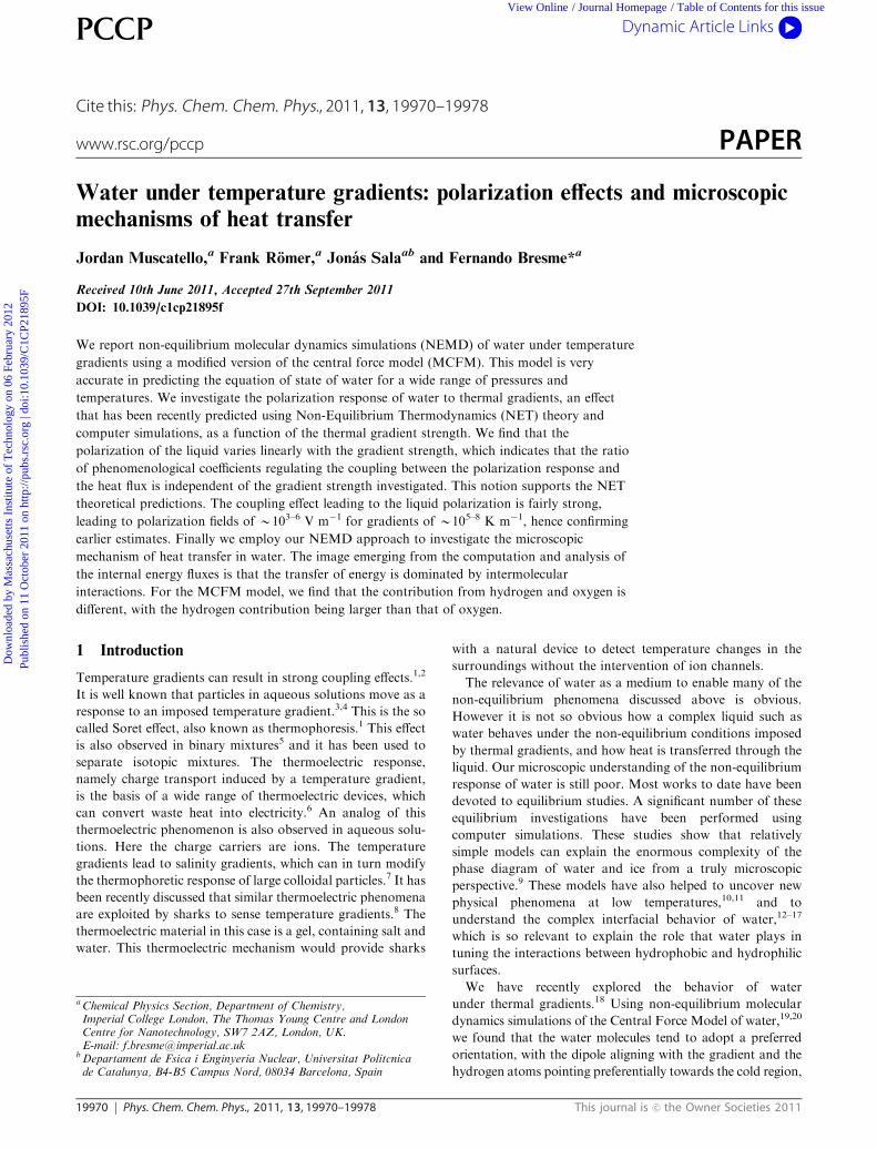
arrangement is shown schematically in Fig. 1.
In the stationary state a heat flux is set up in the system. The
heat flux can be quantified through a microscopic expression,
first derived by Irving and Kirkwood,32 and extended to ionic
systems in ref. 25,
JU;TOTðlÞ ¼ JU;KIN:ðlÞ þ JU;POT:ðlÞ þ JU;COL:ðlÞ
¼ 1
2V
XN2li¼1
miðvi � vÞ2ðvi � vÞ þ 1
V
XN2li¼1
fiððvi � vÞ
� 1
2V
XN2li¼1
XNjai
½ðvi � vÞ � Fij�rij
ð12Þ
which gives the flux in a test volume of volume V located at
layer l. mi and vi are the mass and velocity of particle i,
respectively, fi is the potential energy of particle i, Fij is the
force between particles i and j at distance rij and v is the
barocentric velocity, which in our simulations is zero as the net
momentum of the simulation box is also zero. We note that the
JU,TOT(l) should be constant in the present simulations. This is
true outside the thermostat layers. In that region JU,TOT(l)
features a plateau (see below). We use this plateau to estimate
the energy flux in the gradient direction, JU,f.
In addition, the heat flux can be estimated by using the
following continuity equation,
JU;c ¼ � DU2dtA
; 0; 0
� �ð13Þ
where A is the cross-sectional area of the simulation cell, DU is
the energy removed(�)/added(+) to the cold/hot layers,
and dt is the time step, which was set to 0.3 fs in order to
ensure good numerical stability in the integration of the fast
intramolecular degrees of freedom.
The simulations involved an initial equilibration period of
45 ps to reach a temperature of 325 K across the whole system
cell, and a further 45 ps of nonequilibrium simulation in order
for the system to reach the stationary state. The results
Fig. 1 Snapshot of a representative simulation showing the heat flux
along the simulation box. The color scale indicates the local temperature
of the water molecules. Simulation box dimensions {x,y,z} = {19.725,
19.725, 98.625} A. The location of the hot (425 K) and cold (225 K,
middle of the box) thermostats is also shown.
Table 1 Summary of the systems simulated in this work. JU,f and JU,c correspond to the average flux obtained from eqn (12) and (13) respectively.rT represents the average temperature gradient over the whole simulation cell, andrTT=325 K the local gradient at T= 325 K. The averages anduncertainties reported for the pressure were obtained from an ensemble average over the whole simulation box, and the uncertainty for JU,f wasestimated from the analysis of the flux profiles reported in Fig. 6
DT/K rT/(K A�1) rTT=325 K/(K A�1) P/bar JU,f/(W m�2) JU,c/(W m�2) rT=325 K/(g cm�3) |Ex,T=325 K|/(108 V m�1)
300–350 1 1.06 � 0.06 308.5 � 3.4 8.3 � 0.2 � 109 8.04 � 0.73 � 109 1.0001 2.79 � 0.9275–375 2 2.01 � 0.06 351.3 � 5.3 1.57 � 0.02 � 1010 1.49 � 0.06 � 1010 1.003 6.07 � 1.2250–400 3 2.92 � 0.05 416 � 3.5 2.26 � 0.01 � 1010 2.22 � 0.06 � 1010 1.004 8.34 � 0.6225–425 4 3.88 � 0.05 495.6 � 7.6 2.97 � 0.02 � 1010 2.84 � 0.06 � 1010 1.008 13.49 � 0.6325–475 3 — 1354 � 10 2.46 � 0.03 � 1010 2.34 � 0.1 � 1010 — —250–350 2 1.93 � 0.08 120 � 11 1.4 � 0.02 � 1010 1.6 � 0.1 � 1010 0.9919 6.2 � 1.2
Dow
nloa
ded
by M
assa
chus
etts
Ins
titut
e of
Tec
hnol
ogy
on 0
6 Fe
brua
ry 2
012
Publ
ishe
d on
11
Oct
ober
201
1 on
http
://pu
bs.r
sc.o
rg |
doi:1
0.10
39/C
1CP2
1895
F
View Online
This journal is c the Owner Societies 2011 Phys. Chem. Chem. Phys., 2011, 13, 19970–19978 19973
presented below were obtained from 4–10 simulation runs
consisting of 106 molecular dynamics steps, spanning a total of
1.5–3.0 ns. These simulations were used to estimate averages
and statistical errors. A summary of all the simulations
performed in this work is given in Table 1.
4 Results
4.1 Equation of state and thermal conductivity
Before we discuss our results for water polarization, we
analyze the accuracy of the MCFM model in predicting the
equation of state and thermal conductivity of water for
different pressure and temperature conditions (see Table 1).
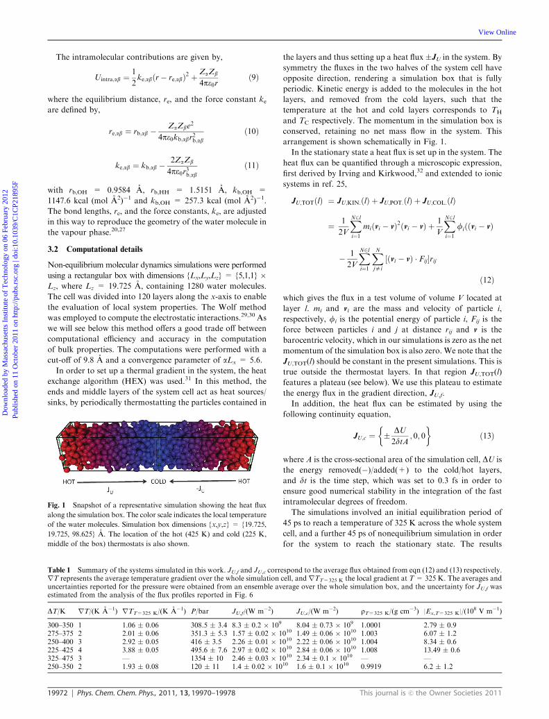
The NEMD method preserves mechanical equilibrium, i.e.,
the pressure along the box is constant (see Fig. 2, top panel).
For each of these average pressures, the system develops
temperature and density gradients. The analysis of these pairs
of quantities at specific regions in the cell, along with the
hypothesis of local equilibrium (see e.g. ref. 25 for an investigation
considering ionic and non polar fluids), provides a route to
construct the equation of state at specific isobars using a single
simulation. The non-equilibrium simulated equation of state is
compared with the corresponding experimental data in Fig. 2. We
performed a running average over 2–4 consecutive layers to
represent these data and in order to reduce the noise associated
to the volume used to sample the densities along the simulation
box. The different isobars were obtained from individual
non-equilibrium simulations, at different pressure and different
gradients, i.e., covering several temperature intervals (see Table 1).
The agreement with experimental results is excellent at the
lower pressures investigated here o500 bars. The accuracy is
comparable to that of two of the most popular force-fields of
water TIP4P-200533 and SPC/E,34 which model the water
molecule as a rigid triangle.w The MCFM model correctly
predicts the large change in density associated to the increase in
temperature and pressure. At very high pressures, B1.3 kbar,
it shows good agreement with the experiment at high
temperatures (450 K) and deviates from the experiment, about
1%, at lower temperatures (350 K). This region of the phase
diagram has been traditionally less investigated via computer
simulations, although data using the TIP4P-2005 have been
reported very recently.35 At high pressures, the TIP4P-2005
model shows excellent agreement with the experimental equation
of state, whereas the SPC/E model slightly underestimates the
pressure at higher temperatures. Overall the level of accuracy of
the MCFM and the SPC/E is comparable at this pressure, with
the SPC/E performing better at low temperatures and the
MCFM better at higher temperatures.
In the following we discuss our results for the thermal
conductivity (TC) of the MCFM model. The TC can be
obtained from Fourier’s law, Jq � JU,c = �lrT, where Jq is
the macroscopic heat flux, which is strictly equal to the
computed internal energy flux, JU,c, in the absence of mass
flux, i.e., in our simulation conditions. In order to obtain
better statistics the symmetry of the simulation cell was
exploited by taking the average of each side about the point
Lx/2, effectively ‘‘folding’’ the simulation cell in half. The
thermal conductivity was then calculated for each layer in
the ‘‘folded’’ cell, using the numerical derivative of the
temperature profile (rT) and the imposed heat flux, according
to Fourier’s Law stated above. We note that the local
temperature gradient must be compatible with the local thermo-
dynamic state defined by the pairs temperature/density at the
constant pressure of the simulation. Hence, assuming a linear
gradient for the whole temperature profile would provide only an
average estimate of the thermal conductivity of the liquid. We
have thus devised a strategy to extract the local thermal
conductivity from our simulations. In all cases the thermal
conductivity was obtained using the temperature gradient
calculated from the temperature profile in the x-direction
Fig. 2 (Top) Pressure profile along the simulation box for three
different non-equilibrium simulations (the symbols have the same
meaning as in Fig. 2, bottom). Dashed lines represent the average
pressure for the whole simulation box. The pressure profile was
obtained from the virial equation. (Bottom) Equation of state
predicted by the MCFM of water at different pressures, obtained
directly from the non-equilibrium molecular dynamics simulations.
The symbols represent our simulations results and the lines experi-
mental data.36 Results from NPT simulations performed in this work
for the TIP4P-200533 (crosses) and the SPC/E34 (stars) models are also
shown.
w The simulations for these two models were performed using mole-cular dynamics simulations in the isothermal–isobaric ensemble(N,P,T) with a potential cut-off in both cases of 9 A and long rangecorrections for the pressure. The electrostatic interactions werecomputed using the Ewald summation method. The densities wereobtained from averages over 2 ns.
Dow
nloa
ded
by M
assa
chus
etts
Ins
titut
e of
Tec
hnol
ogy
on 0
6 Fe
brua
ry 2
012
Publ
ishe
d on
11
Oct
ober
201
1 on
http
://pu
bs.r
sc.o
rg |
doi:1
0.10
39/C
1CP2
1895
F
View Online
19974 Phys. Chem. Chem. Phys., 2011, 13, 19970–19978 This journal is c the Owner Societies 2011
and the imposed heat flux calculated using the continuity
equation. For each layer we calculated the local thermal
conductivity using Fourier’s Law. The fluctuations in the
thermal conductivity are proportional to the size of the layer,
being larger for a small layer. Hence we performed a running
average of these thermal conductivities over several layers to
reduce the fluctuations. The running averages were computed
over 15 points. The error bars on each point represent the
error in the temperature and thermal conductivity obtained
from the analysis of the running average, and hence for a
sub-volume of the non-equilibrium cell. We report 8 running
averages for simulations performed with 107 time steps, and
4 for simulations with 4 � 106 time steps (see Fig. 3).
The thermal conductivity was then plotted as a function of
the temperature in each layer. The error in T for each value is
the standard error due to taking the average over a range of
T values corresponding to an interval of 15 points in the data
set. The error in l is again the standard error of the mean plus
the combined error on each data point in the averaging range.
The thermal conductivity of water, as many other properties
for this liquid, is anomalous.37 It increases with temperature at
low temperatures, unlike common liquids where the thermal
conductivity decreases. This behavior has been traditionally
explained as a signature of hydrogen bonding. At low
temperature the hydrogen bonds can store energy resulting
in an increase of thermal conductivity, whereas at high
temperatures the hydrogen bond network is disrupted and
water recovers the normal behavior observed in simple fluids.
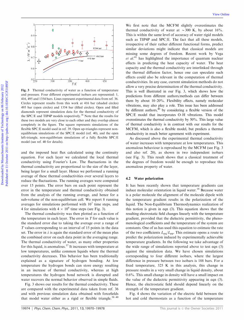
Fig. 3 shows our results for the thermal conductivity. These
are compared with the experimental data taken from ref. 36
and with previous simulation data obtained with forcefields
that model water either as a rigid or flexible triangle.38–40
We first note that the MCFM slightly overestimates the
thermal conductivity of water at B300 K, by about 16%.
This is within the same level of accuracy of water rigid models
such as TIP4P and SPC/E. The fact that all these models,
irrespective of their rather different functional forms, predict
similar deviations might indicate that classical models are
missing some degrees of freedom. Recent work by Vega
et al.41 has highlighted the importance of quantum nuclear
effects in predicting the heat capacity of water. The heat
capacity and the thermal conductivity are interlinked through
the thermal diffusion factor, hence one can speculate such
effects could also be relevant in the computation of thermal
conductivities. In any case, current simulation methods do not
allow a very precise determination of the thermal conductivity.
This is well illustrated in our Fig. 3, which shows how the
predictions from different authors/methods can differ between
them by about 10–20%. Flexibility effects, namely molecular
vibrations, may also play a role. This issue has been addressed
by different authors,40 by considering a flexible version of the
SPC/E model that incorporates O–H vibrations. This model
overestimates the thermal conductivity by 50%. This large value
of thermal conductivity is in contrast with our results for the
MCFM, which is also a flexible model, but predicts a thermal
conductivity in much better agreement with experiment.
As discussed above the experimental thermal conductivity
of water increases with temperature at low temperatures. This
anomalous behaviour is reproduced by the MCFM (see Fig. 3
and also ref. 20), as shown in two independent isobars
(see Fig. 3). This result shows that a classical treatment of
the degrees of freedom would be enough to reproduce this
anomalous property of water.
4.2 Water polarization
It has been recently shown that temperature gradients can
induce molecular orientation in liquid water.18 Because water
is a polar molecule the alignment of the molecule dipole with
the temperature gradient results in the polarization of the
liquid. The Non-Equilibrium Thermodynamics realization of
this notion is given in eqn (3). This equation shows that the
resulting electrostatic field changes linearly with the temperature
gradient, provided that the dielectric permittivity, the pheno-
menological coefficients and the temperature of the system are
constants. One of us has used this equation to estimate the rate
of the two coefficients Lpq/Lpp. This estimate opens a route to
predict the polarization induced by experimentally achievable
temperature gradients. In the following we take advantage of
the wide range of simulations reported above to test eqn (3)
against the simulation data. We have chosen simulations
corresponding to four different isobars, where the largest
difference in pressure between two isobars is 188 bars. For a
fixed temperature, 325 K in this analysis, this change in
pressure results in a very small change in liquid density, about
0.6%. This small change in density will have a small impact on
the value of the dielectric permittivity appearing in eqn (3).
Hence, the electrostatic field should depend linearly on the
strength of the temperature gradient.
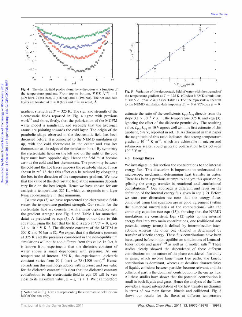
Fig. 4 shows the variation of the electric field between the
hot and cold thermostats as a function of the temperature
Fig. 3 Thermal conductivity of water as a function of temperature
and pressure. Four different experimental isobars are represented: 1,
416, 495 and 1354 bars. Lines represent experimental data from ref. 36.
Circles represent results from this work at 416 bar (shaded circles)
495 bar (open circles) and 1354 bar (filled circles). Open and filled
diamonds represent simulation data for the thermal conductivity of
the SPC/E and TIP4P models respectively.38 Note that the results for
these two models are very close to each other and they overlap almost
completely in the figure. The square represents simulations of the
flexible SPC/E model used in ref. 39. Open up-triangles represent non-
equilibrium simulations of the SPC/E model (ref. 40), and the open
left-triangle, non-equilibrium simulations of a fully flexible SPC/E
model (see ref. 40 for details).
Dow
nloa
ded
by M
assa
chus
etts
Ins
titut
e of
Tec
hnol
ogy
on 0
6 Fe
brua
ry 2
012
Publ
ishe
d on
11
Oct
ober
201
1 on
http
://pu
bs.r
sc.o
rg |
doi:1
0.10
39/C
1CP2
1895
F
View Online
This journal is c the Owner Societies 2011 Phys. Chem. Chem. Phys., 2011, 13, 19970–19978 19975
gradient strength at T = 325 K. The sign and strength of the
electrostatic fields reported in Fig. 4 agree with previous
work18 and show, firstly, that the polarization of the MCFM
water model is significant, and secondly that the hydrogen
atoms are pointing towards the cold layer. The origin of the
parabolic shape observed in the electrostatic field has been
discussed before. It is connected to the NEMD simulation set
up, with the cold thermostat in the center and two hot
thermostats at the edges of the simulation box.z By symmetry
the electrostatic fields on the left and on the right of the cold
layer must have opposite sign. Hence the field must become
zero at the cold and hot thermostats. The proximity between
the cold and the hot layers imposes the parabolic shape. It was
shown in ref. 18 that this effect can be reduced by elongating
the box in the direction of the temperature gradient. We note
that the value of the electrostatic field at the minimum depends
very little on the box length. Hence we have chosen for our
analysis a temperature, 325 K, which corresponds to a layer
lying approximately in that minimum.
To test eqn (3) we have represented the electrostatic fields
versus the temperature gradient strength. Our results for the
electrostatic field are consistent with a linear dependence with
the gradient strength (see Fig. 5 and Table 1 for numerical
data) as predicted by eqn (3). A fitting of our data to this
equation, using the fact that the field is zero at rT = 0, gives
3.1 � 10�2 V K�1. The dielectric constant of the MCFM at
300 K and 70 bar is 82. We expect that the dielectric constant
at 325 K and the pressures considered in the non-equilibrium
simulations will not be too different from this value. In fact, it
is known from experiments that the dielectric constant of
water shows a small dependence with pressure. At our
temperature of interest, 325 K, the experimental dielectric
constant varies from 70 (1 bar) to 75 (1500 bars).42 Hence,
considering this small dependence with pressure and our value
for the dielectric constant it is clear that the dielectric constant
contribution to the electrostatic field in eqn (3) will be very
close to its maximum value, (1 � er�1) E 1. We can therefore
estimate the ratio of the coefficients Lpq/Lqq directly from the
slope 3.1 � 10�2 V K�1, the temperature 325 K and eqn (3),
ignoring the effect of the dielectric permittivity. The resulting
value, Lpq/Lqq E 10 V agrees well with the first estimate of this
quotient, 5–8 V, reported in ref. 18. As discussed in that paper
the magnitude of this ratio indicates that strong temperature
gradients 105�8 K m�1, which are achievable in micron and
submicron scales, could generate polarization fields between
103�6 V m�1.
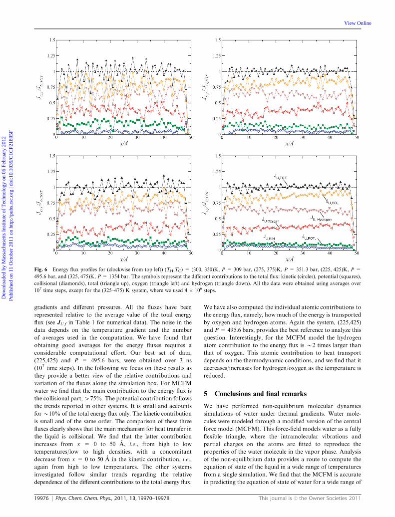
4.3 Energy fluxes
We investigate in this section the contributions to the internal
energy flux. This discussion is important to understand the
microscopic mechanism determining heat transfer in water.
There has been a previous attempt to analyze this question by
splitting the energy transfer in rotational and translational
contributions.43 Our approach is different, and relies on the
definition of the internal energy flux given in eqn (12). Before
we start our discussion we note that the energy fluxes
computed using this equation are in good agreement (within
the numerical uncertainties of the computations) with the
continuity equation (see eqn (13)), showing that the NEMD
simulations are consistent. Eqn (12) splits up the internal
energy flux into two main contributions, one (collisional and
potential energy terms) is defined by intermolecular inter-
actions, whereas the other one (kinetic) is determined by
transfer of kinetic energy. These flux contributions have been
investigated before in non-equilibrium simulations of Lennard-
Jones liquids and gases31,44 as well as in molten salts.25 These
studies clearly showed the dependence of these different
contributions on the nature of the phase considered. Naturally
in gases, which involve large mean free paths, the kinetic
contribution is dominant, whereas at densities characteristics
of liquids, collisions between particles become relevant, and the
collisional part is the dominant contribution to the energy flux.
All these studies have shown that the potential contribution is
small in both liquids and gases. Hence the analysis of the fluxes
provides a simple interpretation of the heat transfer mechanism
in terms of two main factors, kinetic and collisional. Fig. 6
shows our results for the fluxes at different temperature
Fig. 4 The electric field profile along the x-direction as a function of
the temperature gradient. From top to bottom, rT(K A�1) = 1
(309 bar), 2 (351 bar), 3 (416 bar) and 4 (496 bar). The hot and cold
layers are located at x E 0 (hot) and x E 49 (cold) A.
Fig. 5 Variation of the electrostatic field of water with the strength of
the temperature gradient at T = 325 K. (Circles) NEMD simulations
at 308.5 o P/bar o 495.6 (see Table 1). The line represents a linear fit
to the NEMD simulation data imposing Ex = 0 at rTT=325 K = 0.
z Note that in Fig. 4 we are representing the electrostatic field for onehalf of the box only.
Dow
nloa
ded
by M
assa
chus
etts
Ins
titut
e of
Tec
hnol
ogy
on 0
6 Fe
brua
ry 2
012
Publ
ishe
d on
11
Oct
ober
201
1 on
http
://pu
bs.r
sc.o
rg |
doi:1
0.10
39/C
1CP2
1895
F
View Online
19976 Phys. Chem. Chem. Phys., 2011, 13, 19970–19978 This journal is c the Owner Societies 2011
gradients and different pressures. All the fluxes have been
represented relative to the average value of the total energy
flux (see JU,f in Table 1 for numerical data). The noise in the
data depends on the temperature gradient and the number
of averages used in the computation. We have found that
obtaining good averages for the energy fluxes requires a
considerable computational effort. Our best set of data,
(225,425) and P = 495.6 bars, were obtained over 3 ns
(107 time steps). In the following we focus on these results as
they provide a better view of the relative contributions and
variation of the fluxes along the simulation box. For MCFM
water we find that the main contribution to the energy flux is
the collisional part,475%. The potential contribution follows
the trends reported in other systems. It is small and accounts
forB10% of the total energy flux only. The kinetic contribution
is small and of the same order. The comparison of these three
fluxes clearly shows that the main mechanism for heat transfer in
the liquid is collisional. We find that the latter contribution
increases from x = 0 to 50 A, i.e., from high to low
temperatures/low to high densities, with a concomitant
decrease from x = 0 to 50 A in the kinetic contribution, i.e.,
again from high to low temperatures. The other systems
investigated follow similar trends regarding the relative
dependence of the different contributions to the total energy flux.
We have also computed the individual atomic contributions to
the energy flux, namely, how much of the energy is transported
by oxygen and hydrogen atoms. Again the system, (225,425)
and P= 495.6 bars, provides the best reference to analyze this
question. Interestingly, for the MCFM model the hydrogen
atom contribution to the energy flux is B2 times larger than
that of oxygen. This atomic contribution to heat transport
depends on the thermodynamic conditions, and we find that it
decreases/increases for hydrogen/oxygen as the temperature is
reduced.
5 Conclusions and final remarks
We have performed non-equilibrium molecular dynamics
simulations of water under thermal gradients. Water mole-
cules were modeled through a modified version of the central
force model (MCFM). This force-field models water as a fully
flexible triangle, where the intramolecular vibrations and
partial charges on the atoms are fitted to reproduce the
properties of the water molecule in the vapor phase. Analysis
of the non-equilibrium data provides a route to compute the
equation of state of the liquid in a wide range of temperatures
from a single simulation. We find that the MCFM is accurate
in predicting the equation of state of water for a wide range of
Fig. 6 Energy flux profiles for (clockwise from top left) (TH,TC) = (300, 350)K, P = 309 bar, (275, 375)K, P = 351.3 bar, (225, 425)K, P =
495.6 bar, and (325, 475)K, P = 1354 bar. The symbols represent the different contributions to the total flux: kinetic (circles), potential (squares),
collisional (diamonds), total (triangle up), oxygen (triangle left) and hydrogen (triangle down). All the data were obtained using averages over
107 time steps, except for the (325–475) K system, where we used 4 � 106 steps.
Dow
nloa
ded
by M
assa
chus
etts
Ins
titut
e of
Tec
hnol
ogy
on 0
6 Fe
brua
ry 2
012
Publ
ishe
d on
11
Oct
ober
201
1 on
http
://pu
bs.r
sc.o
rg |
doi:1
0.10
39/C
1CP2
1895
F
View Online
This journal is c the Owner Societies 2011 Phys. Chem. Chem. Phys., 2011, 13, 19970–19978 19977
pressures and temperatures. We have further computed the
thermal conductivity at different thermodynamic conditions.
The thermal conductivities at B300 K are overestimated by
about 16%. This is in line with previous simulation results
obtained with the TIP4P and SPC/E models, which represent
water as a rigid triangle. The reason behind this overestimation
of the thermal conductivity is unclear at the moment. Because
our model, MCFM, is flexible, we may expect that the classical
treatment of the vibrational degrees of freedom might have an
impact on the computed thermal conductivities. Simulations of
a rigid version of this model should provide a clue on whether
the thermal conductivity of water can be accurately predicted
using a classical approach or whether other degrees of freedom,
e.g. nuclear effects, must be taken into account. This is a
question that deserves further investigation.
The MCFM reproduces the anomalous increase of the
thermal conductivity with temperature. This effect has been
traditionally interpreted in terms of the temperature dependence
of the energy stored in the hydrogen bond network. We have
shown in this paper that such effect can be reproduced with a
classical model. We also find that this classical model predicts an
increase of the thermal conductivity with pressure in going
fromB400 bar toB1300 bar.We note that the current simulation
approach and the current force-fields are not precise enough to
observe clear trends for smaller pressure ranges, �100 bar.
We have investigated the response of liquid water to
temperature gradients. Non-Equilibrium Thermodynamics
(NET) predicts that a polar fluid should develop a polarization
field as a response to an imposed thermal gradient.18 Further-
more, at constant density and temperature the field should
vary linearly with temperature. We have tested this idea by
performing simulations of the liquid at different temperature
gradient strengths. In agreement with previous work,18 the
MCFM water molecules orient with the dipoles pointing
towards the cold region. We find that the degree of orientation
and the resulting electrostatic field depend linearly on the
gradient, as predicted by NET. This analysis provides an
independent estimate of the ratio of the phenomenological
coefficients, Lpq/Lpp E 10 V for the MCFM model, which is
in good agreement with our previous results.18 This ratio
determines the strength of the polarization field. Strong
gradients, 105�8 K m�1, should produce significant polarization
effects 103�6 V m�1.
Finally, we have investigated the microscopic mechanism of
heat transfer in water by analyzing the total energy flux
contributions. The total energy flux can be split up into two
main contributions. One of them is kinetic, whereas the second
one measures the energy transfer through intermolecular
interactions. We find that intermolecular interactions are the
dominant, 475%, mechanism for heat transfer in water. This
provides a simple microscopic interpretation, where the energy
is transferred through collisions between the atomic sites. This
collisional contribution includes all types of interactions, also
hydrogen bonding. Given the role that hydrogen bonds play
in defining many of the water properties, including the
anomalous properties, it would be very interesting to analyze
the net contribution of hydrogen bonds to the energy flux. We
also find that the hydrogen atoms are more efficient in
transporting heat. This asymmetry in the heat transfer ability
of hydrogen versus oxygen must have a molecular origin,
possibly connected to the molecular geometry of the MCFM
water molecule. Further work is therefore needed to advance
our knowledge on the relationship between heat transfer and
molecular geometry to provide an unequivocal model to
explain the microscopic mechanism of heat transport in water.
Acknowledgements
We would like to acknowledge the Imperial College High
Performance Computing Service for providing computational
resources. Financial support for this work was provided by
The Leverhulme Trust and by the EPSRC through a DTA
scholarship to JM. JS is a recipient of an FPI fellowship from
the Ministerio de Educacion y Ciencia (MEC) of Spain. FB
would like to thank the EPSRC for the award of a Leadership
Fellowship (EP/J003859/1).
References
1 S. R. de Groot and P. Mazur, Non-Equilibrium Thermodynamics,North-Holland, Amsterdam, 1962.
2 S. Kjelstrup and D. Bedeaux, Non-Equilibrium Thermodynamics ofHeterogeneous Systems, World Scientific, Singapore, 2008.
3 S. Duhr and D. Braun, Phys. Rev. Lett., 2006, 96, 168301.4 H.-R. Jiang, H. Wada, N. Yoshinaga and M. Sano, Phys. Rev.Lett., 2009, 102, 208301.
5 C. Debuschewitz and W. Kohler, Phys. Rev. Lett., 2001,87, 055901.
6 G. J. Snyder and E. S. Toberer, Nat. Mater., 2008, 7, 105.7 A. Wurger, Phys. Rev. Lett., 2008, 101, 108302.8 B. R. Brown, Nature, 2003, 421, 495.9 E. Sanz, C. Vega, J. L. F. Abascal and L. G. MacDowell, Phys.Rev. Lett., 2004, 92, 255701.
10 O. Mishima and H. E. Stanley, Nature, 1998, 396, 329.11 P. G. Debenedetti, J. Phys.: Condens. Matter, 2003, 15, R1669.12 L. R. Pratt and A. Pohorille, Chem. Rev., 2002, 102, 2671.13 H. S. Ashbaugh, L. R. Pratt, M. E. Paulaitis, J. Clohecy and
T. L. Beck, J. Am. Chem. Soc., 2005, 127, 2808.14 F. Bresme, E. Chacon and P. Tarazona, Phys. Rev. Lett., 2008,
10, 4704.15 J. Faraudo and F. Bresme, Phys. Rev. Lett., 2004, 92, 236102.16 F. Bresme and A. Wynveen, J. Chem. Phys., 2007, 126, 044501.17 T. G. Lombardo, N. Giovambattista and P. G. Debenedetti,
Faraday Discuss., 2009, 141, 359.18 F. Bresme, A. Lervik, D. Bedeaux and S. Kjelstrup, Phys. Rev.
Lett., 2008, 101, 020602.19 H. L. Lemberg and F. H. Stillinger, J. Chem. Phys., 2001,
115, 7564.20 F. Bresme, J. Chem. Phys., 2001, 115, 7564.21 O. Lehmann, Ann. Phys., 1900, 307, 649.22 I. Janossy, Europhys. Lett., 1988, 5, 431.23 R. D. Astumian, Proc. Natl. Acad. Sci. U. S. A., 2007, 104, 3.24 B. Hafskjold and S. Kjelstrup-Ratkje, J. Stat. Phys., 1995, 78, 463.25 F. Bresme, B. Hafskjold and I. Wold, J. Phys. Chem., 1996,
100, 1879.26 M. Marvan, Czech. J. Phys., 1969, 19, 1240.27 F. Bresme, J. Chem. Phys., 2008, 108, 4505.28 B. Guillot and Y. Guissani, J. Chem. Phys., 1998, 108, 10162.29 D. Wolf, P. Keblinski, S. R. Phillpot and J. Eggebrecht, J. Chem.
Phys., 1999, 110, 8254.30 C. J. Fennell and J. D. Gezelter, J. Chem. Phys., 2006, 124, 234104.31 T. Ikeshoji and B. Hafskjold, Mol. Phys., 1994, 81, 251.32 J. H. Irving and J. G. Kirkwood, J. Chem. Phys., 1950, 18, 817.33 J. L. F. Abascal and C. Vega, J. Chem. Phys., 2005, 123, 234505.34 H. J. C. Berendsen, J. R. Grigera and T. P. Straatsma, J. Phys.
Chem., 1987, 91, 6269.35 J. L. F. Abascal and C. Vega, J. Chem. Phys., 2011, 134, 186101.36 Thermophysical Properties of Fluid Systems, ed. P. Linstrom and
W. Mallard, National Institute of Standards and Technology,
Dow
nloa
ded
by M
assa
chus
etts
Ins
titut
e of
Tec
hnol
ogy
on 0
6 Fe
brua
ry 2
012
Publ
ishe
d on
11
Oct
ober
201
1 on
http
://pu
bs.r
sc.o
rg |
doi:1
0.10
39/C
1CP2
1895
F
View Online
19978 Phys. Chem. Chem. Phys., 2011, 13, 19970–19978 This journal is c the Owner Societies 2011
Gaithersburg MD, 2006, 20899, http://webbook.nist.gov,(retrieved May 29, 2011).
37 D. Eisenberg and W. Kauzmann, The Structure and Properties ofWater, Clarendon Press, Oxford, 2005.
38 D. Bedrov and G. D. Smith, J. Chem. Phys., 2000, 113, 8080.39 W. Evans, J. Fish and P. Keblinski, J. Chem. Phys., 2007,
126, 154504.
40 M. Zhang, E. Lussetti, L. E. S. de Souza and F. Muller-Plathe,J. Phys. Chem. B, 2005, 109, 15060.
41 C. Vega, M. M. Conde, C. McBride, J. L. F. Abascal, E. G. Noya,R. Ramirez and L. M. Sese, J. Chem. Phys., 2010, 132, 046101.
42 M.Uematsu and E.U. Franck, J. Phys. Chem. Ref. Data, 1980, 9, 1291.43 T. Ohara, J. Chem. Phys., 1999, 111, 6492.44 B. Hafskjold and T. Ikeshoji, Mol. Simul., 1996, 16, 139.
Dow
nloa
ded
by M
assa
chus
etts
Ins
titut
e of
Tec
hnol
ogy
on 0
6 Fe
brua
ry 2
012
Publ
ishe
d on
11
Oct
ober
201
1 on
http
://pu
bs.r
sc.o
rg |
doi:1
0.10
39/C
1CP2
1895
F
View Online
Related Documents