Christopher D. Wickens, Jason S. McCarley, Amy L. Alexander

Aviation Human Factors Division

AHFD

Institute of Aviation

University of Illinois at Urbana-Champaign

1 Airport Road Savoy, Illinois 61874

Attention-Situation Awareness (A-SA) Model of Pilot Error

Christopher D. Wickens, Jason S. McCarley,

Amy L. Alexander, Lisa C. Thomas, Michael Ambinder, and Sam Zheng

Technical Report

AHFD-04-15/NASA-04-5

January 2005

Prepared for

NASA Ames Research Center Moffett Field, CA

Contract NASA NAG 2-1535

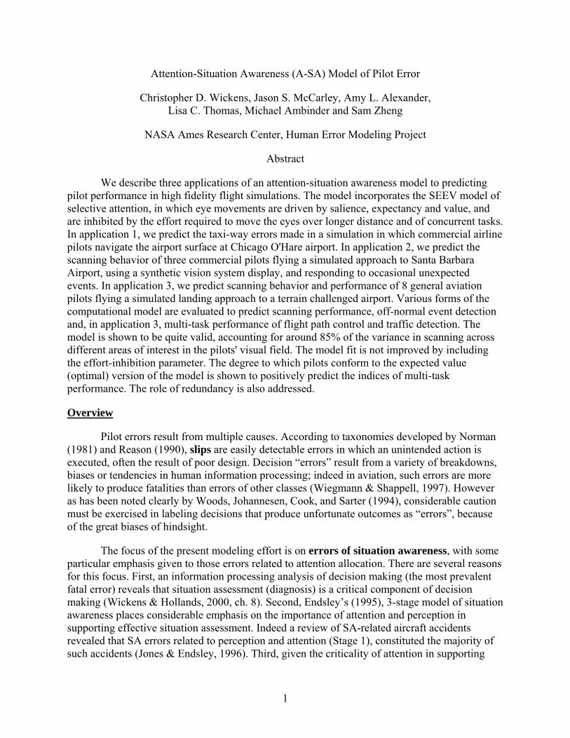
Attention-Situation Awareness (A-SA) Model of Pilot Error

Christopher D. Wickens, Jason S. McCarley, Amy L. Alexander, Lisa C. Thomas, Michael Ambinder and Sam Zheng

NASA Ames Research Center, Human Error Modeling Project

Abstract

We describe three applications of an attention-situation awareness model to predicting pilot performance in high fidelity flight simulations. The model incorporates the SEEV model of selective attention, in which eye movements are driven by salience, expectancy and value, and are inhibited by the effort required to move the eyes over longer distance and of concurrent tasks. In application 1, we predict the taxi-way errors made in a simulation in which commercial airline pilots navigate the airport surface at Chicago O'Hare airport. In application 2, we predict the scanning behavior of three commercial pilots flying a simulated approach to Santa Barbara Airport, using a synthetic vision system display, and responding to occasional unexpected events. In application 3, we predict scanning behavior and performance of 8 general aviation pilots flying a simulated landing approach to a terrain challenged airport. Various forms of the computational model are evaluated to predict scanning performance, off-normal event detection and, in application 3, multi-task performance of flight path control and traffic detection. The model is shown to be quite valid, accounting for around 85% of the variance in scanning across different areas of interest in the pilots' visual field. The model fit is not improved by including the effort-inhibition parameter. The degree to which pilots conform to the expected value (optimal) version of the model is shown to positively predict the indices of multi-task performance. The role of redundancy is also addressed.

Overview

Pilot errors result from multiple causes. According to taxonomies developed by Norman (1981) and Reason (1990), slips are easily detectable errors in which an unintended action is executed, often the result of poor design. Decision “errors” result from a variety of breakdowns, biases or tendencies in human information processing; indeed in aviation, such errors are more likely to produce fatalities than errors of other classes (Wiegmann & Shappell, 1997). However as has been noted clearly by Woods, Johannesen, Cook, and Sarter (1994), considerable caution must be exercised in labeling decisions that produce unfortunate outcomes as “errors”, because of the great biases of hindsight.

The focus of the present modeling effort is on errors of situation awareness, with some particular emphasis given to those errors related to attention allocation. There are several reasons for this focus. First, an information processing analysis of decision making (the most prevalent fatal error) reveals that situation assessment (diagnosis) is a critical component of decision making (Wickens & Hollands, 2000, ch. 8). Second, Endsley’s (1995), 3-stage model of situation awareness places considerable emphasis on the importance of attention and perception in supporting effective situation assessment. Indeed a review of SA-related aircraft accidents revealed that SA errors related to perception and attention (Stage 1), constituted the majority of such accidents (Jones & Endsley, 1996). Third, given the criticality of attention in supporting

1

situation awareness (Sarter & Woods, 1995), it is important to note that some of the most effective computational models of human performance have been developed in the area of attention allocation (Carbonnell, Ward, & Senders, 1968; Moray, 1986; Klatzky, 2000). Fourth, recent analysis has revealed the critical role of attention in the monitoring and supervision of flight deck automation (Parasuraman, Sheridan, & Wickens, 2000; Wickens, 2000; Sklar & Sarter, 1999; Sarter & Woods, 1995; Wickens, Gempler, & Morphew, 2000). Fifth, our laboratory at the Institute of Aviation in Illinois has a long rich history of attention modeling research (e.g., Wickens, 1980; Wickens, Sandry, & Vidulich, 1983; Wickens & Liu, 1988), most recently guided and supported by eye-movement monitoring as a direct index of attention allocation (Bellenkes, Wickens, & Kramer, 1997; Wickens, Helleberg & Xu, 2002, Wickens, Goh, Helleberg, Horrey, & Talleur, 2003). We are able to build upon this in formulating the current model.

Thus the rationale for our focus is as follows: (1) faulty pilot judgment is a critical element for understanding flight safety. (2) Many such faulty judgments result from a breakdown in situation awareness and assessment; that is failure to attend to, and integrate appropriate sources of information. (3) Attention in such contexts is amenable to computational modeling. In the following pages we first described a two component computational model of attention and situation awareness (A-SA), and then discuss three different applications to pilot attention and performance data.

Model Architecture

Foundation of the model. The underlying theoretical structure of the A-SA model is contained in two modules, one governing the allocation of attention to events and channels in the environment, and the second drawing an inference or understanding of the current and future state of the aircraft within that environment. The first module corresponds roughly to Endsley’s (1995) Stage 1 situation awareness, the second corresponds to her Stages 2 and 3. In dynamic systems, there is a fuzzy boundary between Stage 2 (understanding) and Stage 3 (prediction) because the understanding of the present usually has direct implications for the future, and both are equally relevant for the task.

The elements underlying the attention module are contained in the SEEV model of attention allocation, developed by Wickens, Helleberg, Goh, Xu, and Horrey (2001; Wickens, Goh, Helleberg, Horrey, & Talleur, 2003), which can be represented as the probability of attending to an area in visual space, as related to the linear weight of four components:

(1) P(A) = sS - efEF + (ex EX + v V)

Here, coefficients in upper case describe the properties of a display or environment, while those in lower case describe the weight assigned to those properties in the control of an operator’s attention. These elements indicate that the allocation of attention in dynamic environments is driven by bottom-up attention capture of Salient (S) events, is inhibited by the Effort (EF) required to move attention (as well as the effort imposed by concurrent cognitive activity), and is also driven by the expectancy (EX) of seeing valuable (V) events at certain locations in the environment. For example, a high value of expectancy for a given channel (location) means that the channel in question has a high information bandwidth, i.e., events occur frequently on the

2

channel. A high value of weighting for expectancy means that the property of channel bandwidth exerts a strong influence in driving operator’s attention. The name of the SEEV model is derived from the first letter of each of the four boldfaced terms above. An alternative version of the model, to be evaluated below, combines the last two terms of expectancy and value multiplicatively, rather than additively as:

(2) P(A) = sS – efE + ev*EV.

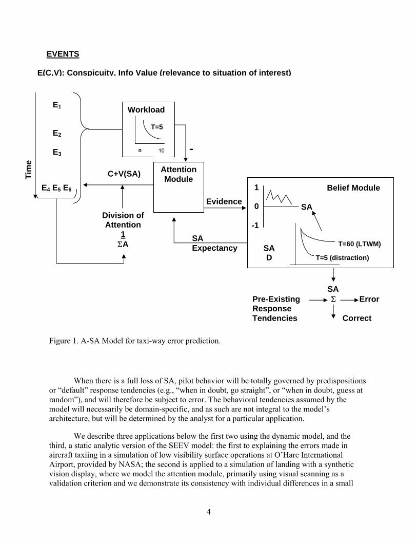
Equations (1) and (2) are static analytic models. Figure 1 contains a more detailed representation of the dynamic form of the full attention and situation awareness (A-SA) components of the process model. As shown in the figure, the model combines two distinct but interacting modules, one of which seeks to represent the attentional processes by which a subject collects information from the environment, the other of which, based on SEEV, seeks to represent the cognitive processes by which attended information is integrated to establish the pilot’s level of situation awareness (SA). The attention component includes elements of the SEEV model, and is also based in part after Luce’s (1959) choice model, and Bundesen’s (1990) Theory of Visual Attention. The decision making component incorporates Hogarth and Einhorn’s (1992) anchoring and adjustment mechanism of belief updating. The product of the total model is a value of SA which ranges between 0 and 1, where 1 indicates perfect SA. This value is used to guide future attentional scanning, and also to determine the likelihood that the pilot will behave correctly (i.e., on the basis of initial planning intentions) when forced to choose between potential actions. In application 1, this choice is what to do at a taxi-way intersection, where errors are frequent.

3

EVENTS E(C,V): Conspicuity, Info Value (relevance to situation of interest)

-

Evidence

E1 E2 E3

E4 E5 E6 C+V(SA) Attention

Module

Division of Attention

1 ΣA

SA Expectancy

Workload

T=5

1

0

-1

SA

SA D T=5 (distraction)

T=60 (LTWM)

0

SA Pre-Existing Σ Error Response Tendencies Correct

Belief Module

Tim

e

10

Figure 1. A-SA Model for taxi-way error prediction.

When there is a full loss of SA, pilot behavior will be totally governed by predispositions or “default” response tendencies (e.g., “when in doubt, go straight”, or “when in doubt, guess at random”), and will therefore be subject to error. The behavioral tendencies assumed by the model will necessarily be domain-specific, and as such are not integral to the model’s architecture, but will be determined by the analyst for a particular application.

We describe three applications below the first two using the dynamic model, and the third, a static analytic version of the SEEV model: the first to explaining the errors made in aircraft taxiing in a simulation of low visibility surface operations at O’Hare International Airport, provided by NASA; the second is applied to a simulation of landing with a synthetic vision display, where we model the attention module, primarily using visual scanning as a validation criterion and we demonstrate its consistency with individual differences in a small

4

number of pilot situation awareness errors. The third is applied to a simulation of SVS landing trials, where we both model the attention module and examine its implications for performance, and we offer a full validation.

Application 1: Aircraft Taxi Errors

The application of the model to predicting taxiway turning errors in an O’Hare Airport simulation study is described in more detail in Wickens and McCarley (2001).

Attention module. In this application pilots are assumed to encounter “events” as they progress along the taxiway. Each event can be characterized by its salience or conspicuity and its value in supporting awareness of where the pilot is (or which way he should turn) along the taxiway. Each parameter is coded within a range of 0 to 1.0. As represented in the attention module, to the left of Figure 1, attention to any given event is inversely proportional to the number of competing events, perceived concurrently, and also perceived recently (with an impact diminishing over time). Attention is influenced by salience, which is maximum for auditory events (Spence & Driver, 2000), and diminishes for visual events as these are available further in peripheral vision.

Attention within the model is considered to be a graded resource which can be allotted in different quantities to different items. The proportion of attention allotted to an item is determined by the item’s attentional weight relative to the summed attentional weights of all items that have been encountered. Situation awareness (SA) is assumed to guide attention allocation in a manner such that a high level of SA serves to guide scanning toward stimuli or events which are themselves conducive to high SA and away from stimuli degrading of SA. This tendency captures the influence of top-down factors such as expectancy and the confirmation bias on evidence seeking.

Belief updating module. SA is updated any time an item or group of items is encountered. The change in belief effected by the items encountered at a given time step is determined by a weighted mean of the value V of each of those items, with the V for a given item weighted by the attentional allotment of that item. This weighted mean will be referred to as the net evidentiary value (NV) for the time step. After the NV has been determined for a given time step, SA is updated via an anchoring and adjustment process like that described by Hogarth and Einhorn (1992). Thus the current value of SA is adjusted upward or downward in accordance with the NV of the newly encountered evidence. As noted by Hogarth and Einhorn (1992), belief updating via such an anchoring-and-adjustment process captures the effects of order of information presentation (i.e., anchoring and recency effects) on information integration.

After SA has been updated in response to the evidence encountered within a given one-second interval, the model proceeds to the next interval using the newly calculated value of SA. If additional evidence is encountered, SA is again updated as per the processes described above. Across intervals wherein no evidence encountered, SA is assumed to decay. The decline of SA in the absence of new evidence is intended to reflect the fact that preservation of SA is a resource-demanding process requiring rehearsal and that, even in low workload situations, such rehearsal is not likely to be continuous. Because the active attentive processing of irrelevant items is likely to interfere with rehearsal in working memory more strongly than is the presence of unattended

5

background stimuli or the demand to maintain a non-attention demanding behavior, the model assumes a faster decay rate for SA during attentional processing of events irrelevant to the SA task at hand (time constant = 5 sec) than during the absence of attention demanding stimuli (time constant = 60 sec, based on analysis of Ericsson and Kintsch’s (1995) model of long-term working memory).

Finally, we assume that the variance in SA that occurs across choice points will make it more or less likely that choice behavior will be based on processed event information (increases when SA is high), or that choices will be based on analyst-specified pre-existing response tendencies such as “when in doubt turn toward the terminal” (increases influence when SA is low). Behavior which is not based on processed event information may be erroneous.

“Validation” application. In the application of the data to predicting taxiway errors, described fully in Wickens and McCarley (2001; see NASA, 2001), we coded the video and audio tapes of a typical pilot during the simulation run, noting the time at which certain “events” occurred, and coding the salience and evidentiary value of each, as indicated by the prototype in Table 1. This allowed us to compute a value of SA at each point in time, increasing with relevant events, and degrading with the passage of time – slowly when nothing else was occurring and rapidly in the presence of irrelevant distracting events (see the “irrelevant discussion” at time 45 of Table 1).

Table 1. Example of scenario time line for taxi-way application.

Time (sec) Object/Event Salience Evidentiary Value

00 Rehearsal of instructions 1.0 1.0 20 Irrelevant discussion 1.0 0.0 30 2-Way Crossing 0.5 0.5 32 Sign 0.5 0.5 35 Sign 0.5 0.5 40 Branch 1.0 0.5 45 Irrelevant Discussion 1.0 0.0 48 3-way crossing 1.0 0.5 48 3-way crossing 1.0 0.5 50 Visually salient traffic 1.0 0.0 52 Visually non-salient traffic 0.5 0.0 58 Point at which pilot should exit 1.0 1.0

6

SA was assumed to reflect the probability that the pilot, when reaching a choice point (e.g., a two- or three-way crossing in Table 1), would recognize the correct response option and behave appropriately as a result. In cases where high SA did not lead the pilot to choose the correct response option, the pilot was assumed to select randomly from among the options available. The probability of a correct choice was thus equal to the probability of the pilot choosing correctly because he/she recognized the correct option (good SA), plus the probability that the pilot failed to recognize the correct option as such (poor SA) but happened to guess correctly among the N options.

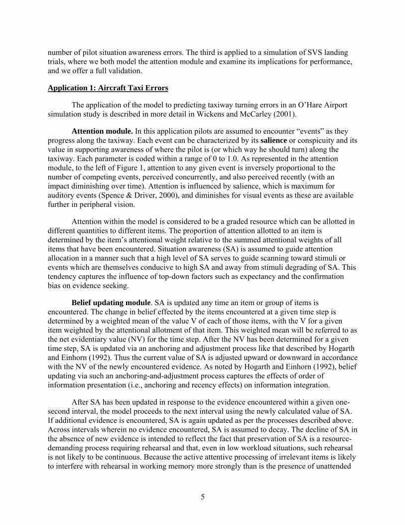
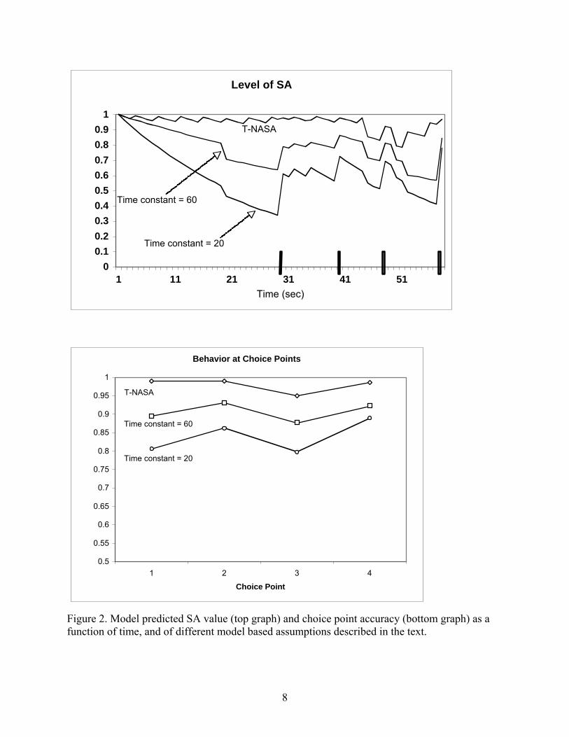
In this application, we did not actually use the model to predict performance (i.e., to validate against errors made). Rather, we ran the model through various iterations to show how SA and choice accuracy would wax and wane across time, and to demonstrate how these changes would be influenced by changes in model parameters such as varying the impact of salience or decay rate. Figure 2 provides an example showing SA variation over time (top graph) and choice point accuracy (1-error rate: bottom graph). The discrete events in Table 1 are reflected as discontinuities in the SA graph of Figure 2. Importantly, as reflected in Figure 2, we included a run in which pilots’ SA could be accurately updated by a T-NASA display within the cockpit (Hooey & Foyle, 2001). The high level of SA, and low rate of choice point errors that are predicted as a result, correspond nicely to the values obtained by pilots in pilot-in-the-loop simulation data, when the T-NASA display was available.

7

Level of SA

00.10.20.30.40.50.60.70.80.9

1

1 11 21 31 41 51Time (sec)

T-NASA

Time constant = 60

Time constant = 20

Behavior at Choice Points

0.5

0.55

0.6

0.65

0.7

0.75

0.8

0.85

0.9

0.95

1

1 2 3 4

Choice Point

T-NASA

Time constant = 60

Time constant = 20

Figure 2. Model predicted SA value (top graph) and choice point accuracy (bottom graph) as a function of time, and of different model based assumptions described in the text.

8

Application 2: Situation Awareness Supported by Synthetic Vision Systems (SVS). The NASA Simulation

The focus of our second effort was to apply the A-SA model to a very different sort of data, describing the performance of pilots making simulated approaches to the Santa Barbara Airport with and without the support of a synthetic vision system (SVS) display (Prinzel et al., 2004; Wickens et al., 2004a, 2004b, 2004c). The scenario is described in Goodman et al. (2003). Several characteristics of this new validation effort required us to modify our modeling approach from that used in the application above. First, unlike the relatively frequent taxi-way errors, obvious loss-of-SA incidents were scarce in the data provided by NASA. Second, we did not have available any explicit or implicit “probes” of SA (e.g., SAGAT) that might have availed data for modeling. Third, although we were provided with a full set of data records in both video and digital files, these revealed few discrete “events” that could be directly tied to the gains or losses of SA in the manner that events (intersection choice and signage) from the taxiway data were. With fewer “events” it became more difficult to employ the salience component of the SEEV model, since salience serves the model only to the extent that it can be defined as a direct property of a discrete event.

To compensate for these shortcomings of the data set, we were provided with an extensive set of eye-movement data, which, in contrast to the first application taxi-data, we could now model directly as the output of our attention module. In addition, while we did not have events defined by salience, we did have available information channels defined by distinct locations. Following the precedence of our previous scanning model approaches (e.g., Wickens et al., 2003) we define these channels as Areas of Interest (AOIs). Each AOI can be defined in terms of a (1) transition to it, or “visit” (from another AOI), (2) dwell duration on the AOI before leaving it, and (3) percentage dwell time (PDT) looking at it (which is the product of the frequency of visits and the mean dwell duration, divided by the total amount of time). We can think of the PDT as a measure of the relative attentional interest of an AOI. While we could not model the salience of events, we were able to model the effort of moving attention (transitioning) from one AOI to another, assuming that such effort is monotonically related to the distance between AOIs. Furthermore, since the approach/landing task is one that has been often studied within the aviation domain, we were able to define the value of tasks on the well established hierarchy of aviate > navigate (Wickens et al., 2003).

Following the procedures developed in Wickens et al. (2003), the value of an AOI was equal to the Value of the task served by the AOI multiplied by the relevance of that AOI to the task in question. The expectancy for information contained in the AOI was determined by bandwidth of the AOI. Thus we were able to estimate the quantitative parameters necessary to determine how frequently an AOI should have been visited, and to predict how frequently it would be visited given the inhibiting influence of effort (which inhibits scans over wide visual angles).

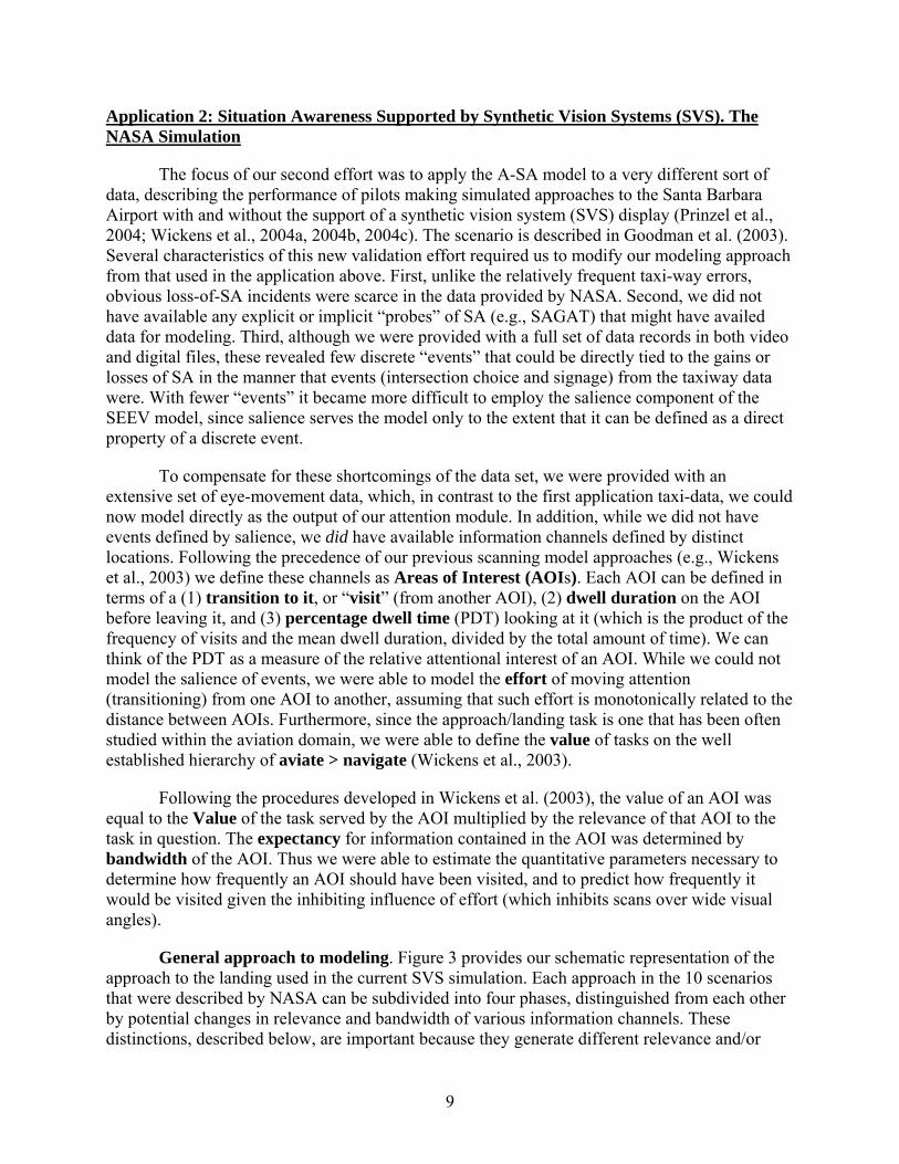
General approach to modeling. Figure 3 provides our schematic representation of the approach to the landing used in the current SVS simulation. Each approach in the 10 scenarios that were described by NASA can be subdivided into four phases, distinguished from each other by potential changes in relevance and bandwidth of various information channels. These distinctions, described below, are important because they generate different relevance and/or

9

bandwidth values for the different AOIs, and hence make different model predictions of P(A), which can be correlated against the observed percentage dwell time.

• Ph 1. Above 1000 ft. Regular “steady state” flight.

• Ph 2. 1000 ft – 850 feet. Lined up on runway (whether visible or not).

• Ph 3. 850-600 feet. Runway becomes visible as the airplane drops below the cloud ceiling in most IMC (low visibility) scenario landings (the exception being the missed approach scenario when the runway is not in sight because of low visibility below this minimum altitude).

• Ph 4. Below 600 feet. Runway remains hidden in low-visibility missed approach scenarios.

Figure 3. Schematic representation of scenario time line.

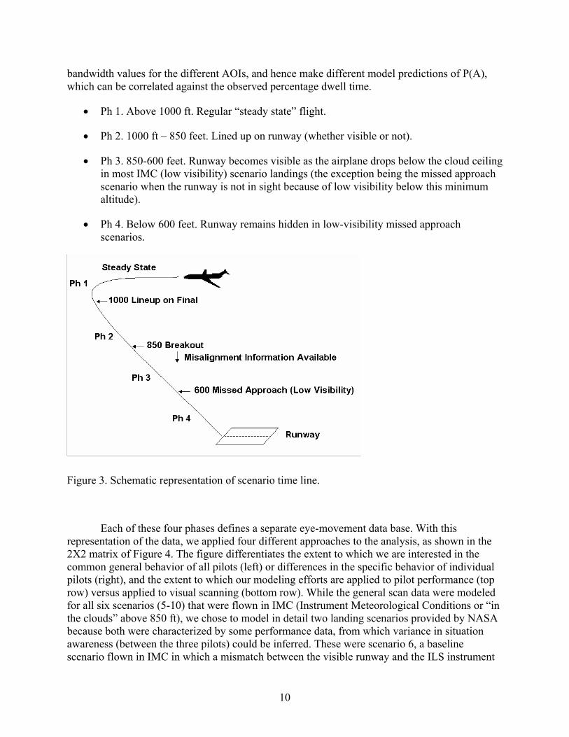
Each of these four phases defines a separate eye-movement data base. With this representation of the data, we applied four different approaches to the analysis, as shown in the 2X2 matrix of Figure 4. The figure differentiates the extent to which we are interested in the common general behavior of all pilots (left) or differences in the specific behavior of individual pilots (right), and the extent to which our modeling efforts are applied to pilot performance (top row) versus applied to visual scanning (bottom row). While the general scan data were modeled for all six scenarios (5-10) that were flown in IMC (Instrument Meteorological Conditions or “in the clouds” above 850 ft), we chose to model in detail two landing scenarios provided by NASA because both were characterized by some performance data, from which variance in situation awareness (between the three pilots) could be inferred. These were scenario 6, a baseline scenario flown in IMC in which a mismatch between the visible runway and the ILS instrument

10

landing guidance forced a go-around below 850 feet, and scenario 10, in which the same mismatch was reflected in a misalignment between the SVS display location of the runway, and the actual runway view outside.

Figure 4. Different approaches to data analysis.

In the upper right cell of Figure 4, the quality of situation awareness was operationally defined by the speed with which pilots became aware of the misalignment in the two scenarios. Careful review of the video tapes and transcriptions revealed that in both scenarios, pilot 5 maintained good SA, rapidly noticing the misalignment and executing the missed approach, whereas pilots 3 and 4 either noticed this discrepancy only after a considerable delay, or not at all, needing to be reminded by the confederate first officer. The distinction between the two “classes” of pilot behavior (“good” and “bad” SA) was important, allowing us to discriminate their attention allocation behavior, as we describe below.

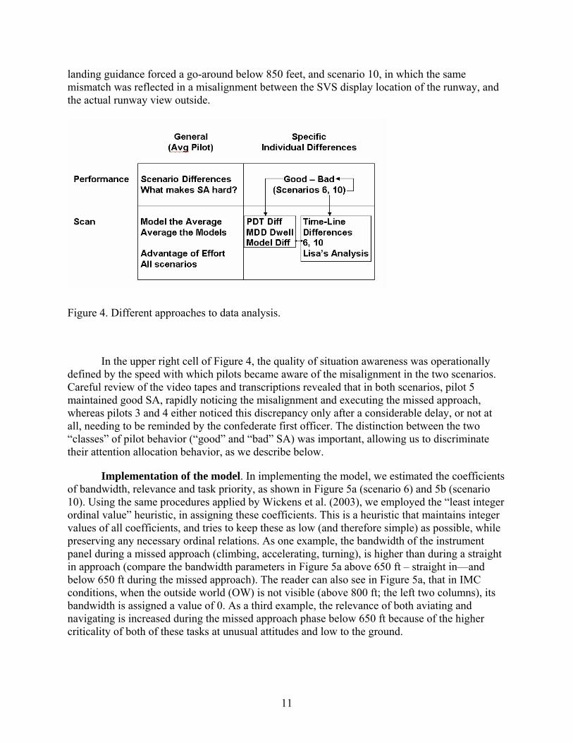
Implementation of the model. In implementing the model, we estimated the coefficients of bandwidth, relevance and task priority, as shown in Figure 5a (scenario 6) and 5b (scenario 10). Using the same procedures applied by Wickens et al. (2003), we employed the “least integer ordinal value” heuristic, in assigning these coefficients. This is a heuristic that maintains integer values of all coefficients, and tries to keep these as low (and therefore simple) as possible, while preserving any necessary ordinal relations. As one example, the bandwidth of the instrument panel during a missed approach (climbing, accelerating, turning), is higher than during a straight in approach (compare the bandwidth parameters in Figure 5a above 650 ft – straight in—and below 650 ft during the missed approach). The reader can also see in Figure 5a, that in IMC conditions, when the outside world (OW) is not visible (above 800 ft; the left two columns), its bandwidth is assigned a value of 0. As a third example, the relevance of both aviating and navigating is increased during the missed approach phase below 650 ft because of the higher criticality of both of these tasks at unusual attitudes and low to the ground.

11

In addition to these parameters, integer parameters for effort were assigned on the basis of the distance between displays in all pairwise comparisons, as extracted from Goodman et al. (2003, Figure 3). Laterally adjacent displays imposed an effort value of 1, vertically separated displays, an effort value of 2, and the presence of an intervening display also imposed an effort value of 2.

Using a version of the SEEV model in which:

(3) P(A) = -Ef + EV

12

(That is, no salience component, and multiplicative relation between expectancy and value), our dynamic model calculated the attractiveness of an AOI as a direct function of the product of its bandwidth and relevance (the latter, modulated by the value of the task to which it was relevant). To this product was added a value of 3 minus the effort required to reach that channel from the currently-attended AOI. This manipulation increased the attentional weight of stimuli whose access required little effort. Thus, when effort needed to reach an AOI was minimal (a value of 0), attentional weight of the object was increased by 3. When the effort needed to reach an AOI was maximal (a value of 3), attentional weight of the object was not increased relative to the value established based on bandwidth and relevance. The probability with which attention shifted to a given AOI was finally calculated by dividing the attentional weight of the AOI by the summed attentional weights of all AOIs.

In our model, the relevance of an AOI remained the same after a fixation as before, and the model could either move to another AOI or remain on the AOI with a probability that was related to the relative attentional weights of all available AOIs (including that of the current fixation). In this way, the eye could remain for a long dwell on a single AOI of high relevance.

Thus, for each phase of flight (characterized by its unique set of values as shown for two of the scenarios in Figure 5), the model generated an N x N transition probability table, where N was set equal to the number of “active” AOIs. For example, as can be seen in Figure 5a in scenario 6 (baseline), N was equal to 3 (Instrument panel, IP, navigational display ND, and Outside World, OW), whereas in Figure 5b (SVS) N was equal to 4, since the SVS display itself defined a now-active AOI

In validating our dynamic model, we were able to derive the PDT directly by summing the total time of dwells on each AOI and dividing by total trial time for all AOIs. We were then able to correlate this model-derived measure with the actual scanning behavior extracted from the eye movement records of each pilot, in each of the 4 phases of each scenario. This analysis was done first for the average pilot, then for each pilot individually.

Modeling the average pilot. We computed the model fitting correlations, based on four different versions of the PDT predictions. These four versions involved the presence or absence of the effort parameter, and involved either correlating model predictions with the average scanning behavior of the 3 pilots, or averaging the correlation values {r} across the three pilots. From this exercise a large number of correlations (model fit) values were produced, as reported in Wickens, McCarley, and Thomas (2004). Through the analyses of these correlations, we drew the following two conclusions:

1. Methodologically, the correlation with the average pilot scan data (average across phases and scenarios r = 0.79) is greater than the average of the pilot correlations (r = 0.60).

2. The inclusion of the Effort parameter offers no benefit to model fitting, and in fact, in some cases, actually reduces the fit. We conclude from this, that pilots were not inhibited from making longer scans, if there was valuable and high-bandwidth information to be obtained at the more distant AOI. Such a conclusion was also consistent with one drawn by Wickens et al. (2003). However a decision was made to retain the effort parameter in

13

our subsequent modeling efforts because of its cognitive plausibility, and because it could be valuable in modeling individual differences between pilots.

We subsequently decided to proceed by modeling all individual IMC (low visibility) scenarios. For each, we could compute the correlation between the predicted and obtained PDT (probability of attention allocation).

The correlational data of all scenarios again reveal the generally higher correlations for the model of the average subject, than for the average of subject models. More important however, are the following two observations.

• The average subject model fits, along with the model fits of individual pilots are all generally good, with positive correlations generally in the 0.60 to 0.80 range, although there are some exceptions. In particular, scenario 6 shows lower correlations. One possibility is that scenario 6 had only two pilots contributing eye movement data, and one of these (pilot 3) had very poor individual fits on all three phases. This point will be important below. There does not appear to be any common feature that might discriminate higher correlations from lower ones (i.e., later versus earlier phases, or SVS versus non SVS scenarios).

• A review of the scatter plots of the individual pilot data included in Wickens, McCarley and Thomas (2004) appeared to reveal one consistent trend, which would account for a drop in the correlations. That is, often when the correlation is low, it is because OW scanning occurs much more frequently than predicted by the model, whereas rarely if ever is out the window (OW) scanning done less than predicted. There are two possible explanations for this. First, in flight phases 1 and 2, the OW is invisible (IMC, see Figure 3), and our model therefore predicts no “relevance” of the OW for either aviating or navigating tasks (see Figure 5). However it is likely that a vigilant pilot, knowing that visibility will be required for landing, will occasionally glance to the OW to assess whether anything is visible. Second, in phases 3 and 4, when the OW is visible (in all but scenarios 5 and 9, which were missed approaches because of the low clouds), it could reflect the fact that the OW was used both for aviating (the true horizon, rather than the instrument panel or SVS horizon) as well as navigating (the true runway, rather than the SVS runway), thereby increasing the “relevance” coefficients from the lower values that we assumed in Figure 5. The use of redundant sources will be explored in application 3.

Modeling individual pilot differences: Validation of SA predictions. As we discussed above, there appeared to be differences between pilots in their awareness of the runway offsets in scenarios 6 and 10. Hence we also asked if differences in the model fits, as reflected by the correlations, might have accounted for the distinct differences between pilot 5 on the one hand, who appeared on the basis of the offset-noticing performance data, to have “good SA”, and pilots 3 and 4, who did not because they either failed to notice, or noticed very late, the misalignments. The data provided only modest support for this distinction. For scenario 6 (baseline ILS display), phase 2, which would characterize the scan pattern just prior to the information regarding the misalignment becoming available, the model fit for pilot 5 (r = .70) is much better than for pilot 3 (r = -.08). (There were no eye movement data for pilot 4.) More detailed examination of these differences revealed that pilot 5 looked at the PFD (a scan necessary to notice the misalignment),

14

whereas pilot 3 did not look there at all during this phase (see Wickens, McCarley, & Thomas, 2004, Appendix A).

For scenario 6, phase 3, similar findings revealed better model fits for pilot 5 (good SA; r = .98) than for pilot 3 (poor SA; r = -0.17). More detailed examination of the scan records suggests that the lower model fit results because pilot 3 again fails to look at the PFD, where evidence of the misalignment is present. We also examined scenario 10 (SVS display) for differences, but failed to find them. Some evidence, reported in Wickens, McCarley, and Thomas (2004), indicated that the better situation awareness of pilot 5 in this scenario resulted because he maintained longer dwells on the outside world at the specific times when it needed to be compared with the SVS information, to diagnose the presence of the runway offset.

Conclusions: Application 2. From our second application, one major conclusion is that, the effort of making longer scans does not appear to inhibit those scans. That is, the model fit is just as good (if not better), when driven by only bandwidth and relevance, as when effort is included. Such a conclusion is consistent with our findings in previous research (Wickens et al., 2003), that scanning of instrument rated general aviation pilots can be very effectively modeled with only expectancy and value as parameters. As such, it validates the optimality of pilot scanning (Moray, 1986). A second conclusion is inherent in the better model fit of the “good” SA pilot (#5), relative to #3, a discrimination that provides some validation of the model in scenario 6.

Our efforts in the second application area were somewhat thwarted primarily by the fact that we did not have an ample supply of performance data upon which to draw inferences about “situation awareness”. While the two measures we did have, of SA-related delays (“errors”) in noticing offsets were compelling, they were only collected once per pilot, and only three (sometimes two) pilots provided data, thus creating a very small sample upon which to make claims for statistical validity. Nevertheless, this application provided the foundation upon which we could address the modeling effort in our third application.

Application 3: Synthetic Vision Systems (SVS) Modeling Revisited: The Illinois Simulation

In the third application, we applied the A-SA model to the visual scanning data of eight pilots, (certified flight instructors) flying an SVS simulated landing at the University of Illinois, described in detail in Wickens et al. (2004a, 2004b). In a Frasca Simulator, with 120 degree outside world visual display, the eight pilots flew a series of curved step down approaches to the terrain challenged environment around Yosemite National Park. In four different display conditions, presented in counter-balanced order, pilots flew with the displays shown in Figure 6.

15

Overlay Separate

Tunn

el

Dat

alin

k

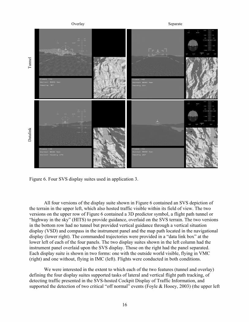
Figure 6. Four SVS display suites used in application 3.

All four versions of the display suite shown in Figure 6 contained an SVS depiction of the terrain in the upper left, which also hosted traffic visible within its field of view. The two versions on the upper row of Figure 6 contained a 3D predictor symbol, a flight path tunnel or “highway in the sky” (HITS) to provide guidance, overlaid on the SVS terrain. The two versions in the bottom row had no tunnel but provided vertical guidance through a vertical situation display (VSD) and compass in the instrument panel and the map path located in the navigational display (lower right). The commanded trajectories were provided in a “data link box” at the lower left of each of the four panels. The two display suites shown in the left column had the instrument panel overlaid upon the SVS display. Those on the right had the panel separated. Each display suite is shown in two forms: one with the outside world visible, flying in VMC (right) and one without, flying in IMC (left). Flights were conducted in both conditions.

We were interested in the extent to which each of the two features (tunnel and overlay) defining the four display suites supported tasks of lateral and vertical flight path tracking, of detecting traffic presented in the SVS-hosted Cockpit Display of Traffic Information, and supported the detection of two critical “off normal” events (Foyle & Hooey, 2003) (the upper left

16

panel in each display suite). (1) A runway offset, similar to that used in application 2 (but only encountered once per pilot, when they landed with the SVS suite). As in application 2, this could only be detected if the pilot looked outside and realized that the SVS display was directing to a landing beside the true runway. (2) A “rogue airplane” trial (Wickens, Helleberg, & Xu, 2002) in which the flight path directed the aircraft to fly directly into the flight of another traffic airplane, one which was only depicted in the outside world, as if its transponder were inactive. All of these provide us with performance measures to be predicted by the model. Visual scanning was measured for all eight pilots. (An additional six pilots completed the simulation, but did not have valid scanning data).

Performance and scanning results. Full details of the performance results are provided in Wickens et al. (2004a, 2004b). Importantly, we found that the two tunnel display suites supported much better flight path tracking performance, and somewhat better traffic detection performance, than did the two display suites using the distributed guidance from VSD on the instrument panel and from the Nav display. We also found that the overlay did not improve tracking performance, and substantially inhibited traffic detection, because of its creation of overlaying clutter. Regarding the off-normal events, in our design eight pilots encountered the rogue blimp while flying with the tunnel. Of these, four detected it and four failed to detect it (as indicated by the absence of any deviation maneuver in their flight path). Only half of these eight pilots had scanning data available, and of these four, there were two “rogue detectors” and two non-detectors. Of the twelve pilots who encountered the runway offset with the SVS display, five failed to notice it.

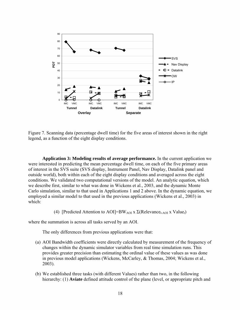
Figure 7 presents the visual scanning behavior of the eight pilots with valid scan data, as a function of the four display conditions, the two visibility conditions (IFR, outside world blank, VFR outside world visible), and the five most important AOIs: the four panels of each display suite shown in Figure 6, and the outside world. The variance across conditions and across AOIs is immediately evident, as is the interaction between these, and these significant effects are described in detail in Wickens et al. (2004a, 2004b). Most importantly, we were able to use these scanning data for our validation of the A-SA scan model, which we describe as follows.

17

0

10

20

30

40

50

60

70

80

90

IMC VMC IMC VMC IMC VMC IMC VMC

PDT

SVS

Nav Display

Datalink

OW

IP

Overlay SeparateTunnel TunnelDatalink Datalink

Figure 7. Scanning data (percentage dwell time) for the five areas of interest shown in the right legend, as a function of the eight display conditions.

Application 3: Modeling results of average performance. In the current application we were interested in predicting the mean percentage dwell time, on each of the five primary areas of interest in the SVS suite (SVS display, Instrument Panel, Nav Display, Datalink panel and outside world), both within each of the eight display conditions and averaged across the eight conditions. We validated two computational versions of the model. An analytic equation, which we describe first, similar to what was done in Wickens et al., 2003, and the dynamic Monte Carlo simulation, similar to that used in Applications 1 and 2 above. In the dynamic equation, we employed a similar model to that used in the previous applications (Wickens et al., 2003) in which:

(4) [Predicted Attention to AOI]=BWAOI x Σ(Relevancet-AOI x Valuet)

where the summation is across all tasks served by an AOI.

The only differences from previous applications were that:

(a) AOI Bandwidth coefficients were directly calculated by measurement of the frequency of changes within the dynamic simulator variables from real time simulation runs. This provides greater precision than estimating the ordinal value of these values as was done in previous model applications (Wickens, McCarley, & Thomas, 2004; Wickens et al., 2003).

(b) We established three tasks (with different Values) rather than two, in the following hierarchy: (1) Aviate defined attitude control of the plane (level, or appropriate pitch and

18

bank). (2) Navigate defined maintaining the plane on the desired course, and climb/descent rate. (3) Hazard awareness defined awareness of the appearance and change of traffic aircraft or terrain.

(c) Unlike application 1, we did not include a salience measure (for the same reasons given for application 2: no discrete events), and unlike application 2, we did not include an effort parameter (because this had been shown in application 2 to be unnecessary to account for scanning of the skilled pilots).

These predictions were validated using the same correlational techniques as employed in application 2.

Table 2 presents the parameter matrix showing bandwidth (of AOI), relevance (of AOI to task) and value (of task) that was established a priori for the experiment. The eight display conditions are listed in the eight columns.

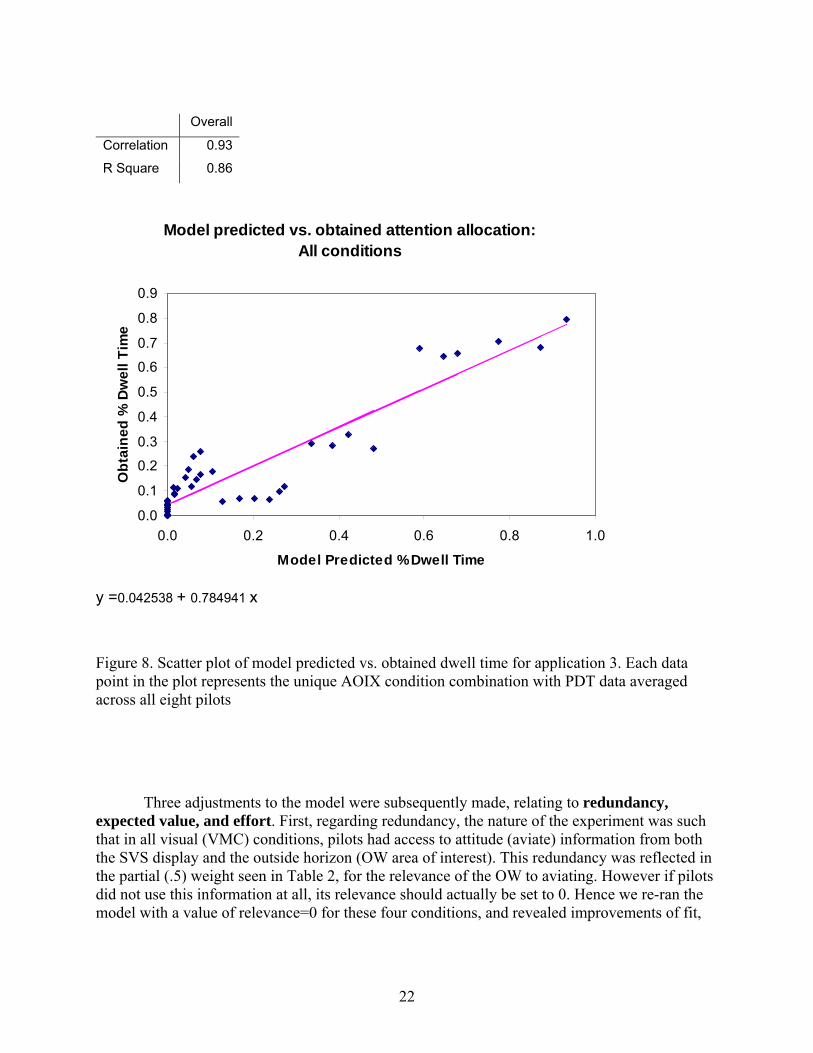
Table 3 presents the predictions from the A-SA equation. The “raw data” predictions, in the top portion of the table were normalized so that, within each condition the total predicted percentage dwells summed to 1.0. These normalized values are presented in the middle portion of the table. The bottom table presents the actual percentage dwell time (PDT) data, identical to those shown in Figure 7 (i.e., averaged over pilots). At the bottom of Table 3, we present the correlations between the model prediction and the obtained PDT values for each condition. These correlations are uniformly positive and, except for the last two conditions, with separated no-tunnel displays, are all above r = .85. Figure 8 presents a scatter plot of the predicted versus obtained PDTs for the five AOIs in all eight conditions collapsed. That is, each point in the scatter plot represents a single unique AOI X condition combination. The correlation reflecting this global prediction is 0.93, capturing 86% of the variance in scanning behavior.

19

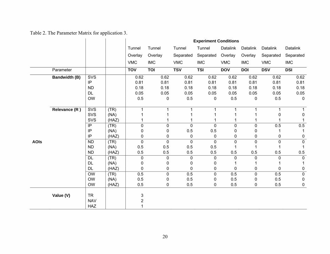
Table 2. The Parameter Matrix for application 3. Experiment Conditions Tunnel Tunnel Tunnel Tunnel Datalink Datalink Datalink Datalink

Overlay Overlay Separated Separated Overlay Overlay Separated Separated

VMC IMC VMC IMC VMC IMC VMC IMC

Parameter TOV TOI TSV TSI DOV DOI DSV DSI

Bandwidth (B) SVS 0.62 0.62 0.62 0.62 0.62 0.62 0.62 0.62 IP 0.81 0.81 0.81 0.81 0.81 0.81 0.81 0.81 ND 0.18 0.18 0.18 0.18 0.18 0.18 0.18 0.18 DL 0.05 0.05 0.05 0.05 0.05 0.05 0.05 0.05 OW 0.5 0 0.5 0 0.5 0 0.5 0 Relevance (R ) SVS (TR) 1 1 1 1 1 1 1 1 SVS (NA) 1 1 1 1 1 1 0 0 SVS (HAZ) 1 1 1 1 1 1 1 1 IP (TR) 0 0 0 0 0 0 0.5 0.5 IP (NA) 0 0 0.5 0.5 0 0 1 1 IP (HAZ) 0 0 0 0 0 0 0 0AOIs ND (TR) 0 0 0 0 0 0 0 0 ND (NA) 0.5 0.5 0.5 0.5 1 1 1 1 ND (HAZ) 0.5 0.5 0.5 0.5 0.5 0.5 0.5 0.5 DL TR) 0 0 0 0 0 0 0 0( DL (NA) 0 0 0 0 1 1 1 1 DL (HAZ) 0 0 0 0 0 0 0 0 OW (TR) 0.5 0 0.5 0 0.5 0 0.5 0 OW (NA) 0.5 0 0.5 0 0.5 0 0.5 0 OW (HAZ) 0.5 0 0.5 0 0.5 0 0.5 0 Value (V) TR 3 NAV 2 HAZ 1

20

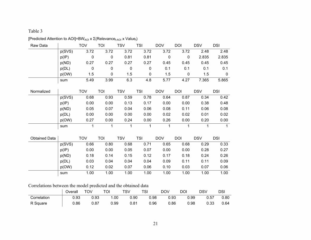
Table 3 [Predicted Attention to AOI]=BWAOI x Σ(Relevancet-AOI x Valuet)

Raw Data TOV TOI TSV TSI DOV DOI DSV DSI p(SVS) 3.72 3.72 3.72 3.72 3.72 3.72 2.48 2.48 p(IP) 0 0 0.81 0.81 0 0 2.835 2.835 p(ND) 0.27 0.27 0.27 0.27 0.45 0.45 0.45 0.45 p(DL) 0 0 0 0 0.1 0.1 0.1 0.1 p(OW) 1.5 0 1.5 0 1.5 0 1.5 0 sum 5.49 3.99 6.3 4.8 5.77 4.27 7.365 5.865

Normalized TOV TOI TSV TSI DOV DOI DSV DSI p(SVS) 0.68 0.93 0.59 0.78 0.64 0.87 0.34 0.42 p(IP) 0.00 0.00 0.13 0.17 0.00 0.00 0.38 0.48 p(ND) 0.05 0.07 0.04 0.06 0.08 0.11 0.06 0.08 p(DL) 0.00 0.00 0.00 0.00 0.02 0.02 0.01 0.02 p(OW) 0.27 0.00 0.24 0.00 0.26 0.00 0.20 0.00 sum 1 1 1 1 1 1 1 1

Obtained Data TOV TOI TSV TSI DOV DOI DSV DSI p(SVS) 0.66 0.80 0.68 0.71 0.65 0.68 0.29 0.33 p(IP) 0.00 0.00 0.05 0.07 0.00 0.00 0.28 0.27 p(ND) 0.18 0.14 0.15 0.12 0.17 0.18 0.24 0.26 p(DL) 0.03 0.04 0.04 0.04 0.09 0.11 0.11 0.09 p(OW) 0.12 0.02 0.07 0.06 0.10 0.03 0.07 0.06 sum 1.00 1.00 1.00 1.00 1.00 1.00 1.00 1.00

Correlations between the model predicted and the obtained data Overall TOV TOI TSV TSI DOV DOI DSV DSI Correlation 0.93 0.93 1.00 0.90 0.98 0.93 0.99 0.57 0.80R Square 0.86 0.87 0.99 0.81 0.96 0.86 0.98 0.33 0.64

21

Overall

Correlation 0.93

R Square 0.86

Model predicted vs. obtained attention allocation: All conditions

0.0

0.1

0.2

0.3

0.4

0.5

0.6

0.7

0.8

0.9

0.0 0.2 0.4 0.6 0.8 1.0

Model Predicted % Dwell Time

Obt

aine

d %

Dw

ell T

ime

y =0.042538 + 0.784941 x

Figure 8. Scatter plot of model predicted vs. obtained dwell time for application 3. Each data point in the plot represents the unique AOIX condition combination with PDT data averaged across all eight pilots

Three adjustments to the model were subsequently made, relating to redundancy, expected value, and effort. First, regarding redundancy, the nature of the experiment was such that in all visual (VMC) conditions, pilots had access to attitude (aviate) information from both the SVS display and the outside horizon (OW area of interest). This redundancy was reflected in the partial (.5) weight seen in Table 2, for the relevance of the OW to aviating. However if pilots did not use this information at all, its relevance should actually be set to 0. Hence we re-ran the model with a value of relevance=0 for these four conditions, and revealed improvements of fit,

22

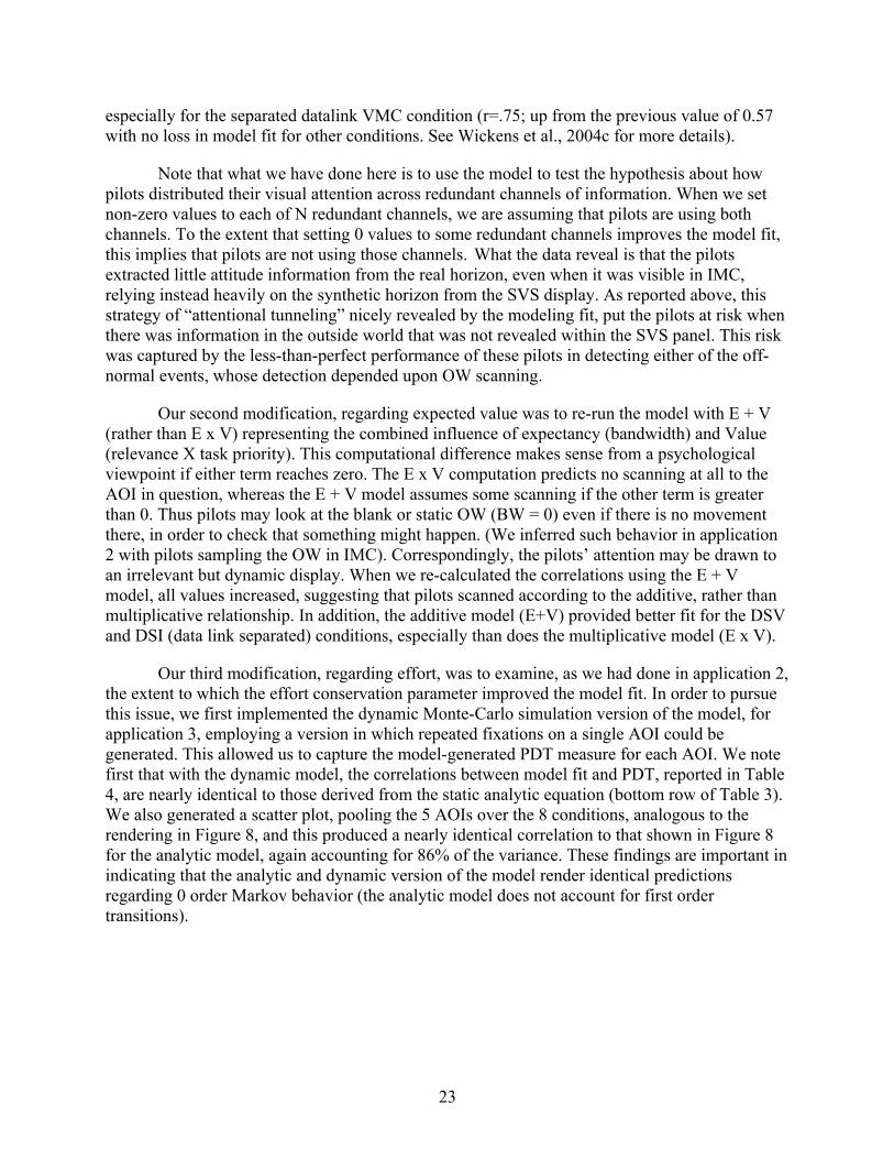
especially for the separated datalink VMC condition (r=.75; up from the previous value of 0.57 with no loss in model fit for other conditions. See Wickens et al., 2004c for more details).

Note that what we have done here is to use the model to test the hypothesis about how pilots distributed their visual attention across redundant channels of information. When we set non-zero values to each of N redundant channels, we are assuming that pilots are using both channels. To the extent that setting 0 values to some redundant channels improves the model fit, this implies that pilots are not using those channels. What the data reveal is that the pilots extracted little attitude information from the real horizon, even when it was visible in IMC, relying instead heavily on the synthetic horizon from the SVS display. As reported above, this strategy of “attentional tunneling” nicely revealed by the modeling fit, put the pilots at risk when there was information in the outside world that was not revealed within the SVS panel. This risk was captured by the less-than-perfect performance of these pilots in detecting either of the off-normal events, whose detection depended upon OW scanning.

Our second modification, regarding expected value was to re-run the model with E + V (rather than E x V) representing the combined influence of expectancy (bandwidth) and Value (relevance X task priority). This computational difference makes sense from a psychological viewpoint if either term reaches zero. The E x V computation predicts no scanning at all to the AOI in question, whereas the E + V model assumes some scanning if the other term is greater than 0. Thus pilots may look at the blank or static OW (BW = 0) even if there is no movement there, in order to check that something might happen. (We inferred such behavior in application 2 with pilots sampling the OW in IMC). Correspondingly, the pilots’ attention may be drawn to an irrelevant but dynamic display. When we re-calculated the correlations using the E + V model, all values increased, suggesting that pilots scanned according to the additive, rather than multiplicative relationship. In addition, the additive model (E+V) provided better fit for the DSV and DSI (data link separated) conditions, especially than does the multiplicative model (E x V).

Our third modification, regarding effort, was to examine, as we had done in application 2, the extent to which the effort conservation parameter improved the model fit. In order to pursue this issue, we first implemented the dynamic Monte-Carlo simulation version of the model, for application 3, employing a version in which repeated fixations on a single AOI could be generated. This allowed us to capture the model-generated PDT measure for each AOI. We note first that with the dynamic model, the correlations between model fit and PDT, reported in Table 4, are nearly identical to those derived from the static analytic equation (bottom row of Table 3). We also generated a scatter plot, pooling the 5 AOIs over the 8 conditions, analogous to the rendering in Figure 8, and this produced a nearly identical correlation to that shown in Figure 8 for the analytic model, again accounting for 86% of the variance. These findings are important in indicating that the analytic and dynamic version of the model render identical predictions regarding 0 order Markov behavior (the analytic model does not account for first order transitions).

23

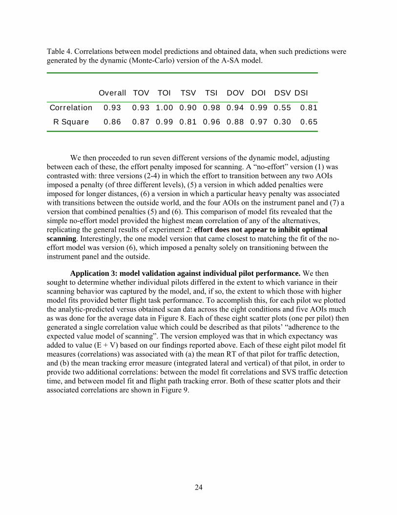
Table 4. Correlations between model predictions and obtained data, when such predictions were generated by the dynamic (Monte-Carlo) version of the A-SA model.

Overall TOV TOI TSV TSI DOV DOI DSV DSI

Correlation 0.93 0.93 1.00 0.90 0.98 0.94 0.99 0.55 0.81

R Square 0.86 0.87 0.99 0.81 0.96 0.88 0.97 0.30 0.65

We then proceeded to run seven different versions of the dynamic model, adjusting between each of these, the effort penalty imposed for scanning. A “no-effort” version (1) was contrasted with: three versions (2-4) in which the effort to transition between any two AOIs imposed a penalty (of three different levels), (5) a version in which added penalties were imposed for longer distances, (6) a version in which a particular heavy penalty was associated with transitions between the outside world, and the four AOIs on the instrument panel and (7) a version that combined penalties (5) and (6). This comparison of model fits revealed that the simple no-effort model provided the highest mean correlation of any of the alternatives, replicating the general results of experiment 2: effort does not appear to inhibit optimal scanning. Interestingly, the one model version that came closest to matching the fit of the no-effort model was version (6), which imposed a penalty solely on transitioning between the instrument panel and the outside.

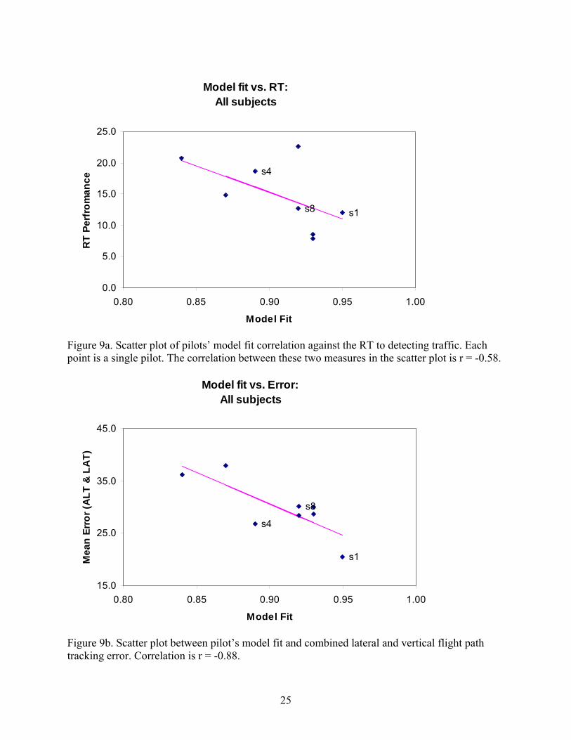
Application 3: model validation against individual pilot performance. We then sought to determine whether individual pilots differed in the extent to which variance in their scanning behavior was captured by the model, and, if so, the extent to which those with higher model fits provided better flight task performance. To accomplish this, for each pilot we plotted the analytic-predicted versus obtained scan data across the eight conditions and five AOIs much as was done for the average data in Figure 8. Each of these eight scatter plots (one per pilot) then generated a single correlation value which could be described as that pilots’ “adherence to the expected value model of scanning”. The version employed was that in which expectancy was added to value (E + V) based on our findings reported above. Each of these eight pilot model fit measures (correlations) was associated with (a) the mean RT of that pilot for traffic detection, and (b) the mean tracking error measure (integrated lateral and vertical) of that pilot, in order to provide two additional correlations: between the model fit correlations and SVS traffic detection time, and between model fit and flight path tracking error. Both of these scatter plots and their associated correlations are shown in Figure 9.

24

Model fit vs. RT: All subjects

s8

s4

s1

0.0

5.0

10.0

15.0

20.0

25.0

0.80 0.85 0.90 0.95 1.00

Model Fit

RT

Perf

rom

ance

Figure 9a. Scatter plot of pilots’ model fit correlation against the RT to detecting traffic. Each point is a single pilot. The correlation between these two measures in the scatter plot is r = -0.58.

Model fit vs. Error: All subjects

s8

s4

s1

15.0

25.0

35.0

45.0

0.80 0.85 0.90 0.95 1.00

Model Fit

Mea

n Er

ror (

ALT

& L

AT)

Figure 9b. Scatter plot between pilot’s model fit and combined lateral and vertical flight path tracking error. Correlation is r = -0.88.

25

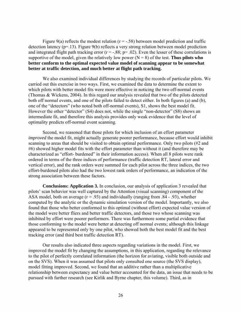
Figure 9(a) reflects the modest relation (r = -.58) between model prediction and traffic detection latency (p=.13). Figure 9(b) reflects a very strong relation between model prediction and integrated flight path tracking error (r = -.88; p= .02). Even the lesser of these correlations is supportive of the model, given the relatively low power (N = 8) of the test. Thus pilots who better conform to the optimal expected value model of scanning appear to be somewhat better at traffic detection, and much better at flight path tracking.

We also examined individual differences by studying the records of particular pilots. We carried out this exercise in two ways. First, we examined the data to determine the extent to which pilots with better model fits were more effective in noticing the two off-normal events (Thomas & Wickens, 2004). In this regard our analysis revealed that two of the pilots detected both off normal events, and one of the pilots failed to detect either. In both figures (a) and (b), one of the “detectors” (who noted both off-normal events), S1, shows the best model fit. However the other “detector” (S4) does not, while the single “non-detector” (S8) shows an intermediate fit, and therefore this analysis provides only weak evidence that the level of optimality predicts off-normal event scanning.

Second, we reasoned that those pilots for which inclusion of an effort parameter improved the model fit, might actually generate poorer performance, because effort would inhibit scanning to areas that should be visited to obtain optimal performance. Only two pilots (#2 and #6) showed higher model fits with the effort parameter than without it (and therefore may be characterized as “effort- burdened” in their information access). When all 8 pilots were rank ordered in terms of the three indices of performance (traffic detection RT, lateral error and vertical error), and the rank orders were summed for each pilot across the three indices, the two effort-burdened pilots also had the two lowest rank orders of performance, an indication of the strong association between these factors.

Conclusions: Application 3. In conclusion, our analysis of application 3 revealed that pilots’ scan behavior was well captured by the Attention (visual scanning) component of the ASA model, both on average (r = .93) and individually (ranging from .84 - .93), whether computed by the analytic or the dynamic simulation version of the model. Importantly, we also found that those who better conformed to this optimal (without effort) expected value version of the model were better fliers and better traffic detectors, and those two whose scanning was inhibited by effort were poorer performers. There was furthermore some partial evidence that those conforming to the model were better at detecting off normal events; although this linkage appeared to be represented only by one pilot, who showed both the best model fit and the best tracking error (and third best traffic detection RT).

Our results also indicated three aspects regarding variations in the model. First, we improved the model fit by changing the assumptions, in this application, regarding the relevance to the pilot of perfectly correlated information (the horizon for aviating, visible both outside and on the SVS). When it was assumed that pilots only consulted one source (the SVS display), model fitting improved. Second, we found that an additive rather than a multiplicative relationship between expectancy and value better accounted for the data, an issue that needs to be pursued with further research (see Kirlik and Byrne chapter, this volume). Third, as in

26

application 2, incorporation of an effort-inhibition parameter does not generally improve model fit, a conclusion that befits well trained expert operators (Moray, 1986).

General Conclusions

The applications of the A-SA model described in this chapter have been defined by two important features: (a) whether a dynamic simulation model of the process was employed (applications 1 and 2), or whether this was coupled with a static analytical equation (application 3), and (b) whether an explicit performance-relevant computation of stage 2 and 3 SA was used (application 1), or whether the focus was primarily on stage 1 SA (visual scanning and information acquisition), using the output of this to predict courser levels of “good” versus “bad” SA-based performance (applications 2 and 3). A third feature was the quality of our validation. Application 1 did not really involve validation at all, but rather, demonstration of the cognitive plausibility of model assumptions. Application 2 involved a weak validation by showing that the model accounted for systematic differences in scanning behavior, and that differences in model fit were associated with some gross differences in pilot performance.

Only in application 3 were we clearly able to conduct a statistical validation of the scanning version of the model, and here our success was quite apparent. Not only did the optimal form of the model predict scanning for all of our pilots, but those who were more optimal were found to perform flight tasks with higher quality. To our knowledge this is the first time that scan model optimality has been explicitly linked to pilot performance in a statistically valid fashion, although others have done so with more qualitative techniques (e.g., Carbonell, Ward, & Senders, 1968; Wickens et al., 2003). The extent to which the improved performance was directly related to component tasks, rather than task (attention) management skills in the multitask environment cannot be determined with certainty, although the latter would appear to be more valid explanation, given the association of situation-awareness and workload in aviation (Wickens, 2002). Noteworthy here is the fact that analyses of the same data base, reported in Wickens et al. (2004b) failed to reveal consistent individual differences linkages between pilot performance and other basic measures of visual scanning (e.g., percentage dwell time on the SVS display). Thus the model serves to incorporate the collective network of scanning forces across various AOIs, in a way that scan measures to a single AOI cannot do, and it is this collective force that drives scanning in an optimal fashion.

There remain at least two important directions in which our modeling effort should proceed. First, our focus has been on the overall percentage dwell time in various AOIs, rather than the mean dwell duration. While these two measures are often correlated, the correlation is not perfect, and the analysis of off-normal failure detection events in application 2 (Wickens, McCarley & Thomas, 2004), certainly suggested some critical distinctions in SA associated with dwell duration. Second, our model explicitly assumes a relatively linear relationship between scanning to a particular AOI and performance. It may be on the other hand that certain large non-linear penalties might be built into zero scans at particular AOIs. That is, for example, the difference between perhaps 0 and 5% scan would have a much greater impact on performance than the difference between 5 and 10%. This approach would incorporate certain non-linear “costs of neglect”, another feature suggested by the fine-grained analysis of the performance of certain pilots in application 3 (see Thomas & Wickens, 2004), and may account for the failure to find our model here, predicting detection of off normal events.

27

On the whole, our results suggest a promising way of looking at how attention supports pilot performance, and how attention allocation breakdowns thwart aviation safety. In projecting the future of aviation, we see a continuous growth in the need for attention models, as advances in automation continue to leave the pilot with less to do, other than to supervise and monitor, via effective attention allocation, the airplane and air space situation under automation control.

Acknowledgments

We wish to acknowledge the contributions of Bill Horrey for assisting with eye-movement analysis, of TJ Hardy, Ron Carbonari and Jonathan Sivier for developing the flight simulation used in application 3, and of Roger Marsh for developing algorithms for eye movement scanning analysis.

References

Bellenkes, A. H., Wickens, C. D., & Kramer, A. F. (1997). Visual scanning and pilot expertise: The role of attentional flexibility and mental model development. Aviation, Space, and Environmental Medicine, 68(7), 569-579.

Bundesen, C. (1990). A theory of visual attention. Psychological Review, 97, 523-547.

Carbonnell, J. F., Ward, J. L., & Senders, J. W. (1968). A queuing model of visual sampling: Experimental validation. IEEE Transactions on Man Machine Systems, MMS-9, 82-87.

Endsley, M. R. (1995). Toward a theory of situation awareness in dynamic systems. Human Factors, 37(1), 85-104.

Ericsson, K. A., & Kintsch, W. (1995). Long-term working memory. Psychological Review, 102, 211-245.

Foyle, D. C., & Hooey, B. L. (2003). Improving evaluation and system design through the use of off-nominal testing: A methodology for scenario development. Proceedings of the Twelfth International Symposium on Aviation Psychology (pp. 397-402). Dayton, OH: Wright State University.

Goodman, A., Hooey, B.L., Foyle, D.C. & Wilson, J.R. (2003). Characterizing visual performance during approach and landing with and without a synthetic vision display: A part-task study. In D. C. Foyle, A. Goodman & B. L. Hooey (Eds.), Conference Proceedings of the 2003 NASA Aviation Safety Program Conference on Human Performance Modeling of Approach and Landing with Augmented Displays (NASA Conference Proceedings NASA/CP-2003-212267).

Hogarth, R. M., & Einhorn, H. J. (1992). Order effects in belief updating: The belief-adjustment model. Cognitive Psychology, 24, 1-55.

Hooey, B. L., & Foyle, D. C. (2001). A post-hoc analysis of navigation errors during surface operations: Identification of contributing factors and mitigating solutions. Proceedings of the 11th Symposium on Aviation Psychology. Columbus, OH: Ohio State University.

Jones, D. G., & Endsley, M. R. (1996). Sources of situation awareness errors in aviation. Aviation, Space, & Environmental Medicine, 67(6), 507-512.

28

Klatzky, R. L. (2000). When to inspect? Recurrent inspection decisions in a simulated risky environment. Journal of Experimental Psychology: Applied, 6(3), 222-235.

Luce, R.D. (1959). Individual choice behavior. New York: Wiley.

Moray, N. (1986). Monitoring behavior and supervisory control. In K. R. Boff, L. Kaufman, & J. P. Thomas (Eds.), Handbook of perception and performance, Vol. II (pp. 40-1-40-51). New York: Wiley & Sons.

National Aeronautics and Space Administration. (2001). Information and data package for human performance modelers: Airport taxi operations with and without T-NASA at Chicago O'Hare. Unpublished documents, NASA Ames Research Center, Human Factors Research & Technology Division.

Norman, D. A. (1981). Categorization of action slips. Psychological Review, 88, 1-15.

Parasuraman, R., Sheridan, T. B., & Wickens, C. D. (2000, May). A model for types and levels of human interaction with automation. IEEE Transactions on Systems, Man, & Cybernetics, 30(3), 286-297.

Prinzel, L. J., III, Comstock, J. R., Jr., Glaab, L. J., Kramer, L. J., Arthur, J. J., & Barry, J. S. (2004). The efficacy of head-down and head-up synthetic vision display concepts for retro- and forward-fit of commercial aircraft. The International Journal of Aviation Psychology, 14(1), 53-77.

Reason, J. (1990). Human error. New York: Cambridge University Press.

Sarter, N. B., & Woods, D. D. (1995). How in the world did we ever get into that mode? Mode error and awareness in supervisory control. Human Factors, 37(1), 5-19.

Sklar, A. E., & Sarter, N. B. (1999). Good vibrations: Tactile feedback in support of attention allocation and human-automation coordination in event-driven domains. Human Factors, 41(4), 543-552.

Spence, C., & Driver, J. (2000). Audiovisual links in attention: Implications for interface design. In D. Harris (Ed.), Engineering psychology and cognitive ergonomics. Hampshire: Ashgate Publishing.

Thomas, L. C., & Wickens, C. D. (2004). Eye-tracking and individual differences in off-normal event detection when flying with a synthetic vision system display. Proceedings of the 48th Annual Meeting of the Human Factors and Ergonomics Society. Santa Monica, CA: Human Factors and Ergonomics Society.

Wickens, C. D. (1980). The structure of attentional resources. In R. Nickerson (Ed.), Attention and performance VIII (pp. 239-257). Hillsdale, NJ: Lawrence Erlbaum.

Wickens, C. D. (2000). The tradeoff of design for routine and unexpected performance: Implications of situation awareness. In M. R. Endsley & D. J. Garland (Eds.), Situation awareness analysis and measurement (pp. 211-225). Mahwah, NJ: Lawrence Erlbaum.

Wickens, C.D. (2002). Situation awareness and workload in aviation. Current Directions in Psychological Science, 11(4), 128-133.

Wickens, C. D., Alexander, A. L., Horrey, W. J., Nunes, A., & Hardy, T. J. (2004b). Traffic and flight guidance depiction on a synthetic vision system display: The effects of clutter on

29

performance and visual attention allocation. Proceedings of the 48th Annual Meeting of the Human Factors and Ergonomics Society. Santa Monica, CA: Human Factors and Ergonomics Society.

Wickens, C. D., Alexander, A. L., Thomas, L. C., Horrey, W. J., Nunes, A., Hardy, T. J., & Zheng, X. S. (2004a). Traffic and flight guidance depiction on a synthetic vision system display: The effects of clutter on performance and visual attention allocation (AHFD-04-10/NASA(HPM)-04-1). Savoy, IL: University of Illinois, Aviation Human Factors Division.

Wickens, C. D., Gempler, K., & Morphew, M. E. (2000). Workload and reliability of predictor displays in aircraft traffic avoidance. Transportation Human Factors Journal, 2(2), 99-126.

Wickens, C. D., Goh, J., Helleberg, J., Horrey, W., & Talleur, D. A. (2003). Attentional models of multitask pilot performance using advanced display technology. Human Factors, 45(3), 360-380.

Wickens, C. D., Helleberg, J., Goh, J., Xu, X., & Horrey, B. (2001). Pilot task management: testing an attentional expected value model of visual scanning (ARL-01-14/NASA-01-7). Savoy, IL: University of Illinois, Aviation Research Laboratory.

Wickens, C. D., Helleberg, J., & Xu, X. (2002). Pilot maneuver choice and workload in free flight. Human Factors, 44(2), 171-188.

Wickens, C. D., & Hollands, J. (2000). Engineering psychology and human performance (3rd ed.). Upper Saddle River, NJ: Prentice Hall.

Wickens, C. D., & Liu, Y. (1988). Codes and modalities in multiple resources: A success and a qualification. Human Factors, 30, 599-616.

Wickens, C. D., & McCarley, J. S. (2001). Attention-situation awareness (A-SA) model of pilot error (Final Technical Report ARL-01-13/NASA-01-6). Savoy, IL: University of Illinois, Aviation Research Lab.

Wickens, C. D., McCarley, J. S. & Thomas, L. (2003). Attention-situation awareness (A-SA) model. In D. Foyle, B. Hooey & A. Goodman (Eds.), Human Performance Modeling Workshop Proceedings. NASA Ames Research Center.

Wickens, C. D., Sandry, D., & Vidulich, M. (1983). Compatibility and resource competition between modalities of input, output, and central processing. Human Factors, 25, 227-248.

Wiegmann, D. A., & Shappell, S. A. (1997). Human factors analysis of postaccident data: Applying theoretical taxonomies of human error. The International Journal of Aviation Psychology, 7(1), 67-82.

Woods, D. D., Johannesen, L. J., Cook, R. I., & Sarter, N. B. (1994). Behind human error: Cognitive systems, computers, and hindsight (State-the-the Art Report CSERIAC 94-01). Wright-Patterson AFB, OH: CSERIAC Program Office.

30