VLSI DSP 2010 Y.H. Hwang 2-1 Chapter 2 Digital Signal Processing Algorithms & Their Representations VLSI DSP 2010 Y.H. Hwang 2-2 Part 1. Review of DSP Algorithms

Welcome message from author
This document is posted to help you gain knowledge. Please leave a comment to let me know what you think about it! Share it to your friends and learn new things together.
Transcript
VLSI DSP 2010 Y.H. Hwang 2-1
Chapter 2 Digital Signal Processing Algorithms & Their Representations
VLSI DSP 2010 Y.H. Hwang 2-2
Part 1.Review of DSP Algorithms
VLSI DSP 2010 Y.H. Hwang 2-3
Example DSP algorithms and applications
Speech Coding/decoding, encryption/decryption
Recognition, synthesis
Digital cellular phones, personal communication systems
digital cordless phones, multimedia computers, secure communication
Modem algorithmsDigital cellular phones, personal communication systems
Digital audio broadcast, wireless computing, navigation
Digital communication, data/fax modems
VLSI DSP 2010 Y.H. Hwang 2-4
Audio equalization, noise cancellationConsumer audio, professional audio, advanced vehicular audio
Echo cancellationSpeakerphones, modems, telephone switches
Digital communication
BeamformingNavigation, radar/sonar, smart antenna
Image compression and decompressionDigital cameras, digital video, multimedia computers, consumer video
Example DSP algorithms and applications
VLSI DSP 2010 Y.H. Hwang 2-5
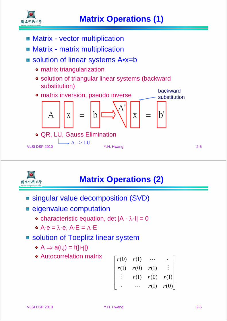
A x = b x = b'A'
backward substitution
A => LU
Matrix Operations (1)
Matrix - vector multiplication
Matrix - matrix multiplication
solution of linear systems A•x=bmatrix triangularization
solution of triangular linear systems (backward substitution)
matrix inversion, pseudo inverse
QR, LU, Gauss Elimination
VLSI DSP 2010 Y.H. Hwang 2-6
⎥⎥⎥⎥
⎦
⎤
⎢⎢⎢⎢
⎣
⎡
⋅
⋅
)0()1(
)1()0()1(
)1()0()1(
)1()0(
rr
rrr
rrr
rr
Matrix Operations (2)
singular value decomposition (SVD)
eigenvalue computationcharacteristic equation, det |A - λ·I| = 0
A·e = λ·e, A·E = Λ·E
solution of Toeplitz linear systemA ⇒ a(i,j) = f(|i-j|)
Autocorrelation matrix
VLSI DSP 2010 Y.H. Hwang 2-7
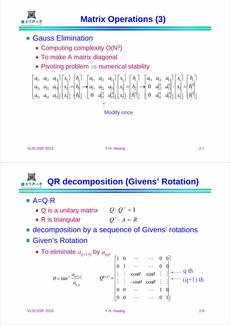
Matrix Operations (3)
Gauss EliminationComputing complexity O(N3)
To make A matrix diagonal
Pivoting problem ⇒ numerical stability
( ) ( ) ( )
( ) ( )
( ) ( )
( )
( )⎥⎥⎥
⎦
⎤
⎢⎢⎢
⎣
⎡=⎥⎥⎥
⎦
⎤
⎢⎢⎢
⎣
⎡⋅⎥⎥⎥
⎦
⎤
⎢⎢⎢
⎣
⎡→⎥⎥⎥
⎦
⎤
⎢⎢⎢
⎣
⎡=⎥⎥⎥
⎦
⎤
⎢⎢⎢
⎣
⎡⋅⎥⎥⎥
⎦
⎤
⎢⎢⎢
⎣
⎡→⎥⎥⎥
⎦
⎤
⎢⎢⎢
⎣
⎡=⎥⎥⎥
⎦
⎤
⎢⎢⎢
⎣
⎡⋅⎥⎥⎥
⎦
⎤
⎢⎢⎢
⎣
⎡
13
12
1
3
2
1
133
132
123
122
131211
13
2
1
3
2
1
133
132
232221
131211
3
2
1
3
2
1
333231
232221
131211
0
0
0 b
b
b
x
x
x
aa
aa
aaa
b
b
b
x
x
x
aa
aaa
aaa
b
b
b
x
x
x
aaa
aaa
aaa
Modify once
VLSI DSP 2010 Y.H. Hwang 2-8
RAQ
QQt
t
=⋅
Ι=⋅
( )
⎥⎥⎥⎥⎥⎥⎥⎥
⎦
⎤
⎢⎢⎢⎢⎢⎢⎢⎢
⎣
⎡
−=
1000
0100
cossin
sincos
0010
0001
,
θθθθpqQ
q th
(q+1) thpq
pq
a
a
,
,11tan +−=θ
QR decomposition (Givens’ Rotation)
A=Q·RQ is a unitary matrix
R is triangular
decomposition by a sequence of Givens’ rotations
Given’s Rotation
To eliminate aq+1,p by aq,p
VLSI DSP 2010 Y.H. Hwang 2-9
⎥⎥⎥⎥
⎦
⎤
⎢⎢⎢⎢
⎣
⎡
−
→
⎥⎥⎥⎥
⎦
⎤
⎢⎢⎢⎢
⎣
⎡
θθθθ
cossin00
sincos00
0010
0001
44434241
34333231
24232221
14131211
aaaa
aaaa
aaaa
aaaa
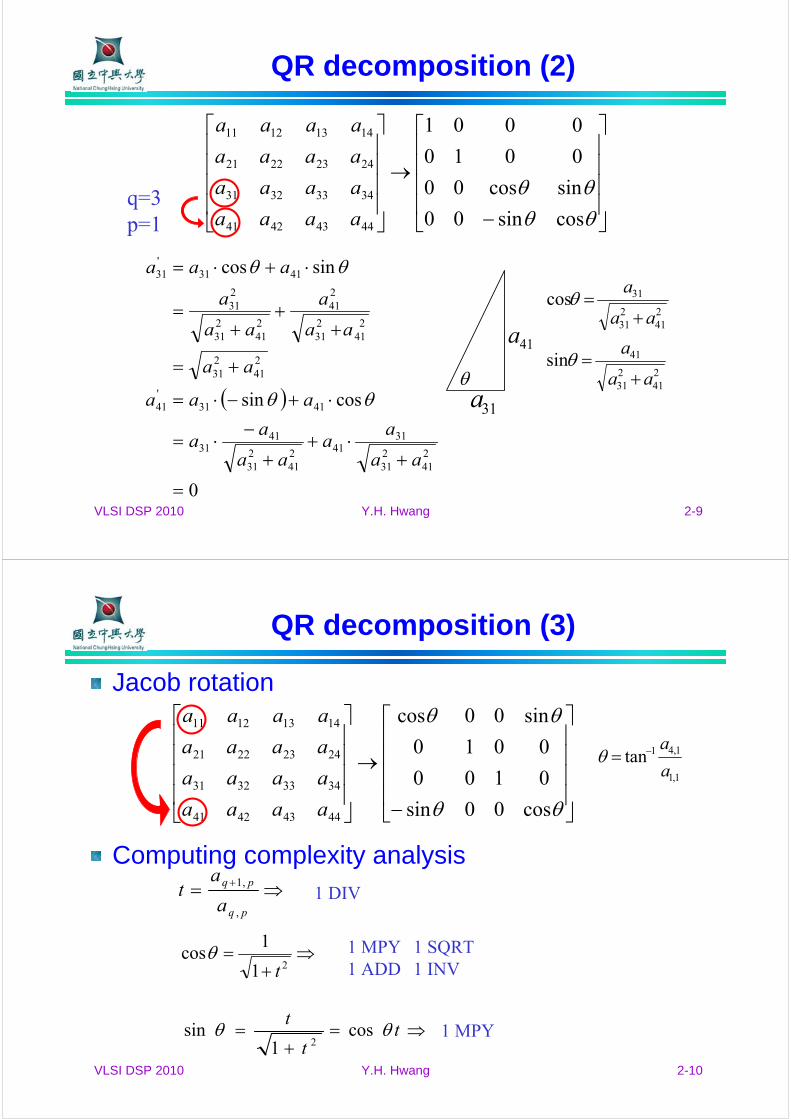
q=3p=1
( )
0
cossin
sincos
241
231
31412
41231
4131
4131'41
241
231
241
231
241
241
231
231
4131'31
=
+⋅+
+
−⋅=
⋅+−⋅=
+=
++
+=
⋅+⋅=
aa
aa
aa
aa
aaa
aa
aa
a
aa
a
aaa
θθ
θθ
θ
41a
31a241
231
41
241
231
31
sin
cos
aa
a
aa
a
+=
+=
θ
θ
QR decomposition (2)
VLSI DSP 2010 Y.H. Hwang 2-10
⎥⎥⎥⎥
⎦
⎤
⎢⎢⎢⎢
⎣
⎡
−
→
⎥⎥⎥⎥
⎦
⎤
⎢⎢⎢⎢
⎣
⎡
θθ
θθ
cos00sin
0100
0010
sin00cos
44434241
34333231
24232221
14131211
aaaa
aaaa
aaaa
aaaa
⇒= +
pq
pq
a
at
,
,1
⇒+
=21
1cos
tθ
⇒=+
= tt
t θθ cos1
sin2
1 MPY 1 SQRT1 ADD 1 INV
1 MPY
QR decomposition (3)
Jacob rotation
Computing complexity analysis
1,1
1,41tana
a−=θ
1 DIV
VLSI DSP 2010 Y.H. Hwang 2-11
⎥⎥⎥⎥⎥⎥
⎦
⎤
⎢⎢⎢⎢⎢⎢
⎣
⎡
x
x
x
x
x
⎥⎥⎥⎥⎥⎥
⎦
⎤
⎢⎢⎢⎢⎢⎢
⎣
⎡
x
x
x
x
x
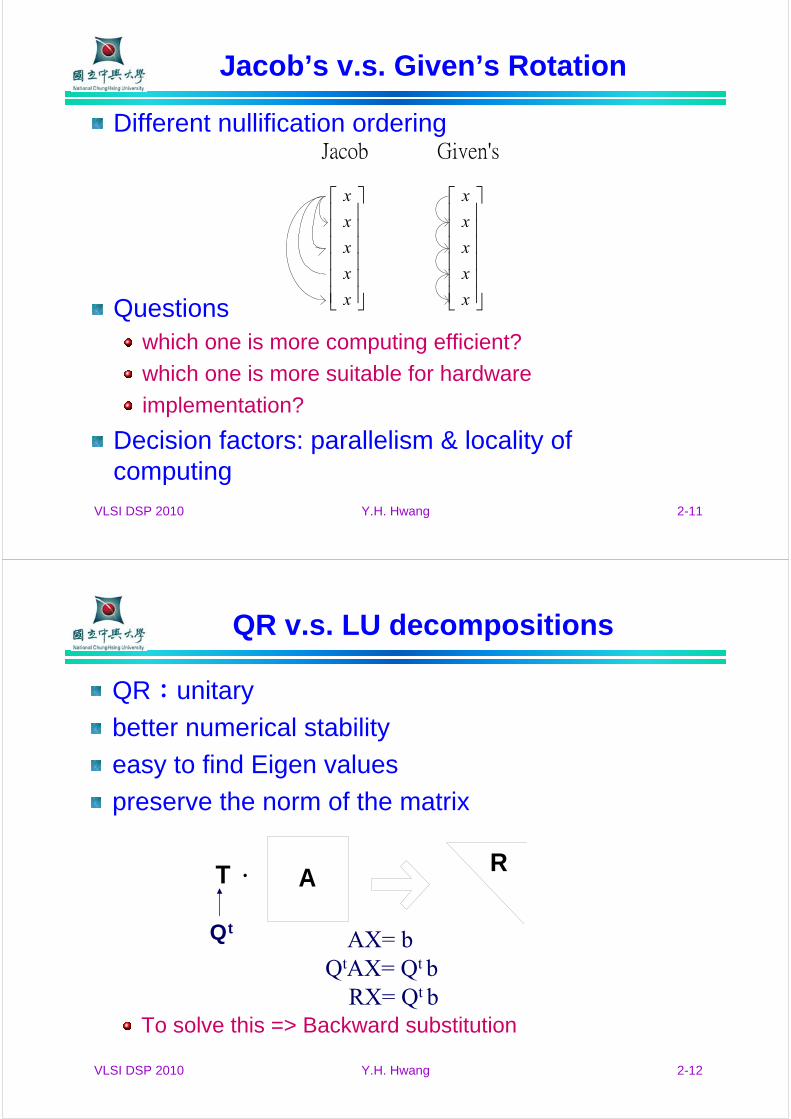
Jacob Given's
Jacob’s v.s. Given’s Rotation
Different nullification ordering
Questionswhich one is more computing efficient?
which one is more suitable for hardware
implementation?
Decision factors: parallelism & locality of computing
VLSI DSP 2010 Y.H. Hwang 2-12
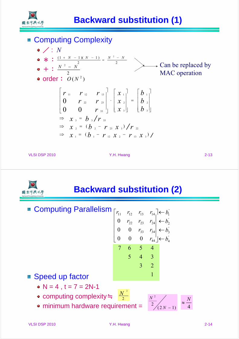
A RT.
QtAX= b
QtAX= Qt bRX= Qt b
QR v.s. LU decompositions
QR:unitary
better numerical stability
easy to find Eigen values
preserve the norm of the matrix
To solve this => Backward substitution
VLSI DSP 2010 Y.H. Hwang 2-13
Backward substitution (1)
Computing Complexity/ : N
*:
+:
order:
xrxrbxrxrbx
rbxbbb
xxx
rrrrrr
31321211
2232322
3333
3
2
1
3
2
1
33
2322
131211
)(
)(
000
−−=⇒
−=⇒
=⇒
⎥⎥⎥⎥
⎦
⎤
⎢⎢⎢⎢
⎣
⎡
=
⎥⎥⎥⎥
⎦
⎤
⎢⎢⎢⎢
⎣
⎡
⋅
⎥⎥⎥⎥
⎦
⎤
⎢⎢⎢⎢
⎣
⎡
22
)1)(11( 2 NNNN −=
−−+
2
2 NN − Can be replaced by MAC operation
)( 2NO
VLSI DSP 2010 Y.H. Hwang 2-14
Backward substitution (2)
Computing Parallelism
Speed up factorN = 4 , t = 7 = 2N-1
computing complexity≒
minimum hardware requirement =2
2
N
)12(2
2
−N
N
1
2 3
3 4 5
4 5 6 7
000
00
0
'4
'3
'2
'1
44
3433
242322
14131211
b
b
b
b
r
rr
rrr
rrrr
←←←←
⎥⎥⎥⎥
⎦
⎤
⎢⎢⎢⎢
⎣
⎡
4
N≈
VLSI DSP 2010 Y.H. Hwang 2-15
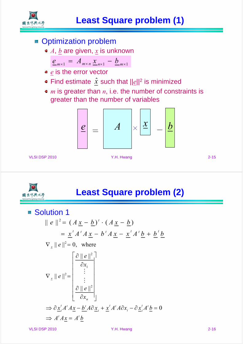
111 ×××× −= mnnmm bxAe
Least Square problem (1)
Optimization problemA, b are given, x is unknown
e is the error vector
Find estimate such that ||e||2 is minimized
m is greater than n, i.e. the number of constraints is greater than the number of variables
x̂
e A x b
VLSI DSP 2010 Y.H. Hwang 2-16
bbbAxxAbxAAx
bxAbxAetttttt
t
+−−=
−⋅−= )()(|||| 2
bAxAA
bAxxAAxxAbxAAx
x
e
x
e
e
e
tt
tt
iitt
ittt
i
n
x
x
=⇒
=∂−∂+∂−∂⇒
⎥⎥⎥⎥⎥⎥⎥
⎦
⎤
⎢⎢⎢⎢⎢⎢⎢
⎣
⎡
∂∂
∂∂
=∇
=∇
0
||||
||||
||||
where,0||||
2
1
2
2
2
Least Square problem (2)
Solution 1
VLSI DSP 2010 Y.H. Hwang 2-17
Least Square problem (3)
Solution 1 (cont.)
If AtA is non-singular, then
is the pseudo inverse of matrix A
Not practical due to the inverse operation
bAxAAbAxAA tttt =⇒=−⇒ 0
tt
tt
AAAA
bAbAAAx1
1
)(
,)(−+
+−
=
==
VLSI DSP 2010 Y.H. Hwang 2-18
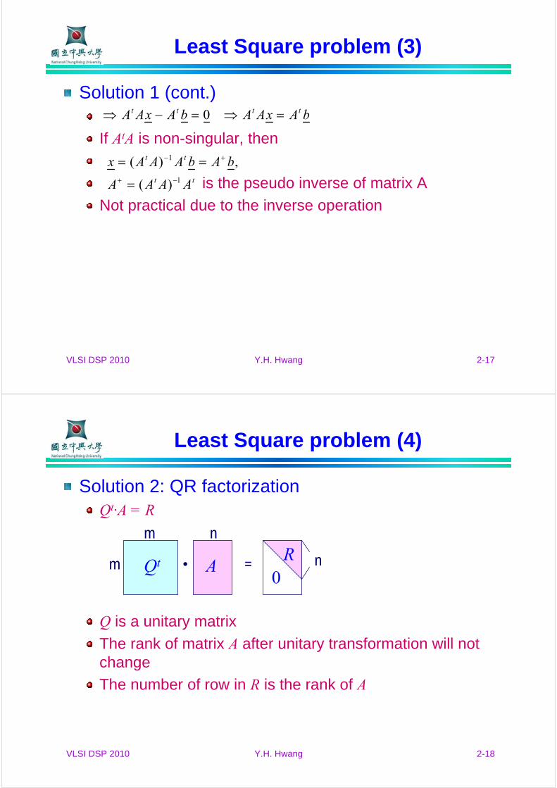
Least Square problem (4)
Solution 2: QR factorizationQt·A = R
Q is a unitary matrix
The rank of matrix A after unitary transformation will not change
The number of row in R is the rank of A
Qt AR
0
m
m
n
n• =
VLSI DSP 2010 Y.H. Hwang 2-19
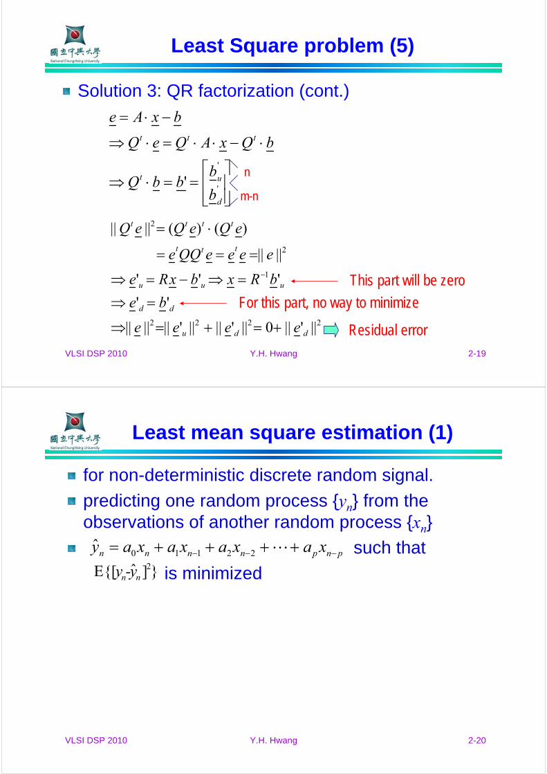
Least Square problem (5)
Solution 3: QR factorization (cont.)
⎥⎥⎦
⎤
⎢⎢⎣
⎡==⋅⇒
⋅−⋅⋅=⋅⇒
−⋅=
'
'
'd
ut
ttt
b
bbbQ
bQxAQeQ
bxAe
n
m-n
2222
1
2
2
||'||0||'||||'||||||
''
'''
||||
)()(||||
ddu
dd
uuu
ttt
tttt
eeee
be
bRxbxRe
eeeeQQe
eQeQeQ
+=+=⇒
=⇒=⇒−=⇒
===
⋅=
− This part will be zero
For this part, no way to minimize
Residual error
VLSI DSP 2010 Y.H. Hwang 2-20
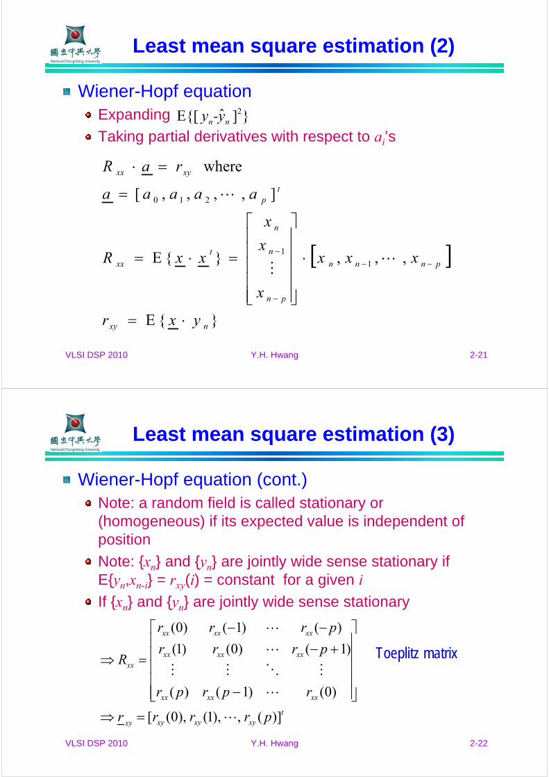
ˆ22110 pnpnnnn xaxaxaxay −−− ++++=
}]ˆE{[ 2nn y-y
Least mean square estimation (1)
for non-deterministic discrete random signal.
predicting one random process {yn} from the observations of another random process {xn}
such that
is minimized
VLSI DSP 2010 Y.H. Hwang 2-21
Least mean square estimation (2)
Wiener-Hopf equationExpanding
Taking partial derivatives with respect to ai’s
[ ]
}{E
,,,}{E
],,,,[
where
1
1
210
nxy
pnnn
pn
n
n
t
xx
tp
xyxx
yxr
xxx
x
x
x
xxR
aaaaa
raR
⋅=
⋅
⎥⎥⎥⎥⎥
⎦
⎤
⎢⎢⎢⎢⎢
⎣
⎡
=⋅=
=
=⋅
−−
−
−
}]ˆE{[ 2nn y-y
VLSI DSP 2010 Y.H. Hwang 2-22
Least mean square estimation (3)
Wiener-Hopf equation (cont.)Note: a random field is called stationary or (homogeneous) if its expected value is independent of position
Note: {xn} and {yn} are jointly wide sense stationary if E{yn,xn-i} = rxy(i) = constant for a given i
If {xn} and {yn} are jointly wide sense stationary
txyxyxyxy
xxxxxx
xxxxxx
xxxxxx
xx
prrrr
rprpr
prrr
prrr
R
)](,),1(),0([
)0()1()(
)1()0()1(
)()1()0(
=⇒
⎥⎥⎥⎥⎥
⎦
⎤
⎢⎢⎢⎢⎢
⎣
⎡
−
+−−−
=⇒ Toeplitz matrix
VLSI DSP 2010 Y.H. Hwang 2-23
∑∑
∑∑
∑ ∑
=
−
=
−
=
−
=
−
= =
−==
=⋅=⇒
+=⇒
−+−=
p
k
kk
q
k
kk
q
k
kk
p
k
kk
p
k
q
kkk
zazAzbzB
zA
zBzHzXzHzY
zXzbzYzazY
knxbknyany
10
01
1 0
1)( ,)(with
)(
)()( where),()()(
)()()(
)()()(
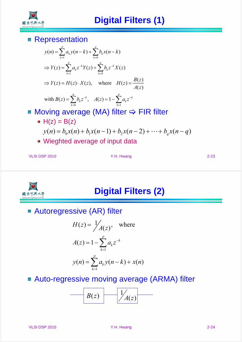
Digital Filters (1)
Representation
Moving average (MA) filter FIR filterH(z) = B(z)
Wieghted average of input data
)()2()1()()( 210 qnxbnxbnxbnxbny q −++−+−+=
VLSI DSP 2010 Y.H. Hwang 2-24
∑
∑
=
=
−
+−=
−=
=
p
kk
p
k
kk
nxknyany
zazA
zAzH
1
1
)()()(
1)(
where,)(1)(
)(1
zA)(zB
Digital Filters (2)
Autoregressive (AR) filter
Auto-regressive moving average (ARMA) filter
VLSI DSP 2010 Y.H. Hwang 2-25
ωαθ(ω) ⋅=
Digital Filters (3)
Linear phase filterPhase shift is proportional to frequency
Fixed delay of each frequency component
Symmetrical coefficients: h(n) = h(N-n)
Ex: h(0) h(1) h(2) h(3) h(4) h(5)
x(n) x(n-1) x(n-2) x(n-3) x(n-4) x(n-5)
∑
∑ ∑∑−
=
−−−−
−
=
−
+
−−−
=
−
+=
+==
21
0
)1(
21
0
1
21
1
0
])[(
)()()()(
N
n
nNn
N
n
N
N
nnN
n
n
zznh
znhznhznhzH
VLSI DSP 2010 Y.H. Hwang 2-26
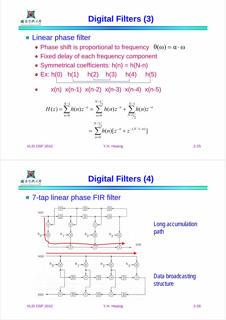
Digital Filters (4)
7-tap linear phase FIR filter
Data broadcastingstructure
Long accumulationpath
VLSI DSP 2010 Y.H. Hwang 2-27
Adaptive Filters
Used for applications such asEcho cancellation, channel equalization, voicebandmodem, digital mobile radio, system identification, ….
The coefficients of the filter are updatedat each iteration to minimize the difference between the output and the desired signalContinues until the coefficients converge
Basic building blocksGeneral filter blockCoefficient update block
Coefficient update subject to different criteriaLMS, RLS, …
VLSI DSP 2010 Y.H. Hwang 2-28
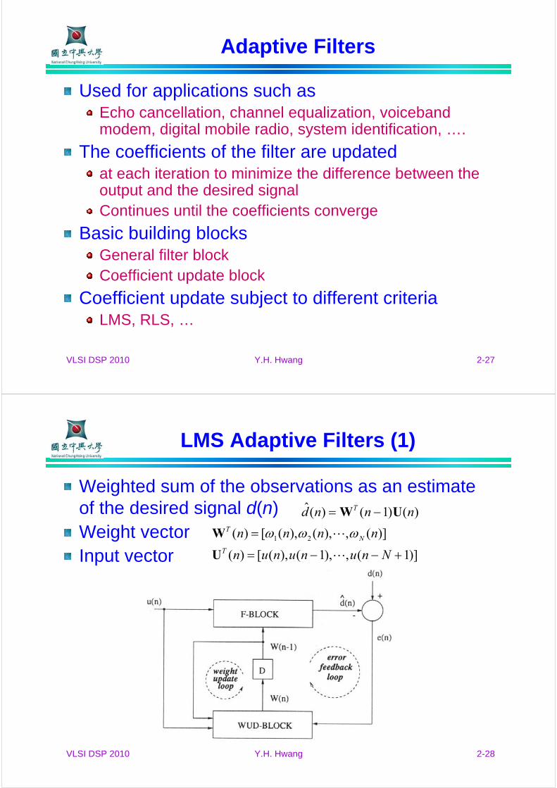
LMS Adaptive Filters (1)
)]1(,),1(),([)(
)](,),(),([)(
)()1()(ˆ
21
+−−=
=
−=
Nnununun
nnnn
nnnd
T
NT
T
U
W
UW
ωωω
Weighted sum of the observations as an estimate of the desired signal d(n)Weight vectorInput vector
VLSI DSP 2010 Y.H. Hwang 2-29
LMS Adaptive Filters (2)
Estimation errorThe difference between the desired signal and the estimated signal
In the nth iteration, WT(n) minimizing the square error e2(n) is selected
Coefficients updateThe derivative of e2(n) w.r.t. WT(n-1)
)()1()()(ˆ)()( nnndndndne T UW −−=−=
)()()1()(
))((2
1)1()(
2)(2
22)(
2
22
nnenn
nenn
ed
de
e
T
T
T
T
T
UWW
WW
UUUW
UUWUW
W
W
⋅+−=⇒
Δ⋅−−=
−=−−=
⋅+−=∂∂
=Δ
μ
μ
VLSI DSP 2010 Y.H. Hwang 2-30
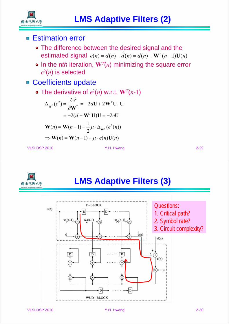
LMS Adaptive Filters (3)
Questions:1. Critical path?2. Symbol rate?3. Circuit complexity?
VLSI DSP 2010 Y.H. Hwang 2-31
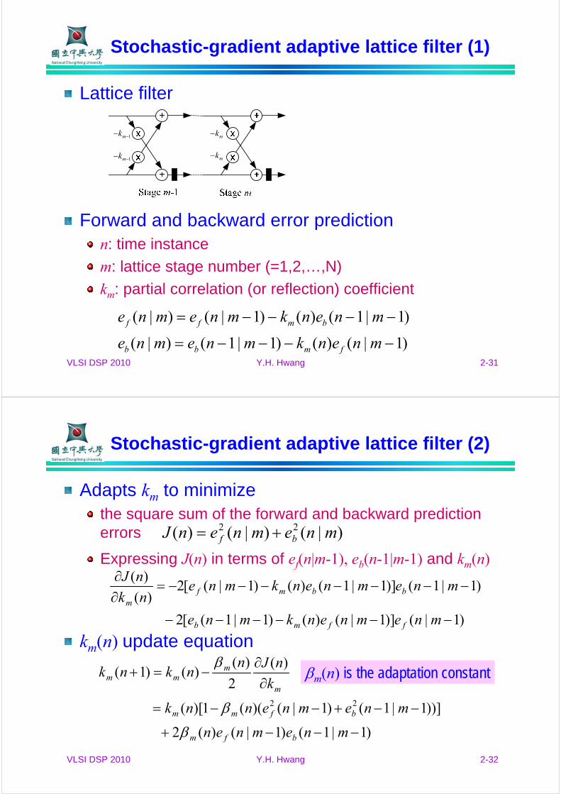
Stochastic-gradient adaptive lattice filter (1)
Lattice filter
Forward and backward error predictionn: time instance
m: lattice stage number (=1,2,…,N)
km: partial correlation (or reflection) coefficient
)1|()()1|1()|(
)1|1()()1|()|(
−−−−=
−−−−=
mnenkmnemne
mnenkmnemne
fmbb
bmff
mk−
mk−
1−− mk
1−− mk
VLSI DSP 2010 Y.H. Hwang 2-32
Stochastic-gradient adaptive lattice filter (2)
Adapts km to minimizethe square sum of the forward and backward prediction errors
Expressing J(n) in terms of ef(n|m-1), eb(n-1|m-1) and km(n)
km(n) update equation
)|()|()( 22 mnemnenJ bf +=
)1|()]1|()()1|1([2
)1|1()]1|1()()1|([2)(
)(
−−−−−−
−−−−−−−=∂∂
mnemnenkmne
mnemnenkmnenk
nJ
ffmb
bbmfm
)1|1()1|()(2
))]1|1()1|()((1)[(
)(
2
)()()1(
22
−−−+
−−+−−=
∂∂
−=+
mnemnen
mnemnennk
k
nJnnknk
bfm
bfmm
m
mmm
β
β
ββm(n) is the adaptation constant
VLSI DSP 2010 Y.H. Hwang 2-33
Stochastic-gradient adaptive lattice filter (3)
Adaptation constant βm(n)To keep adaptation speed independent of the input signal levels
normalized by an estimate of the sum of the (m-1)-th order prediction error variance
β is a constant dependent of the initial value of S(0|m-1)
)1|1()1|(
)1|()1()1|1(
)1|(
1)(
22 −−+−+
−−=−+−
=
mnemne
mnSmnS
mnSn
bf
m
β
β
VLSI DSP 2010 Y.H. Hwang 2-34
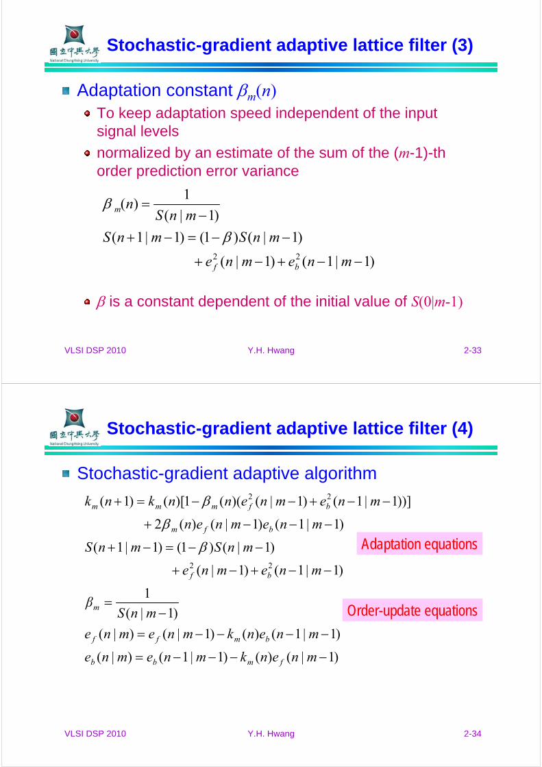
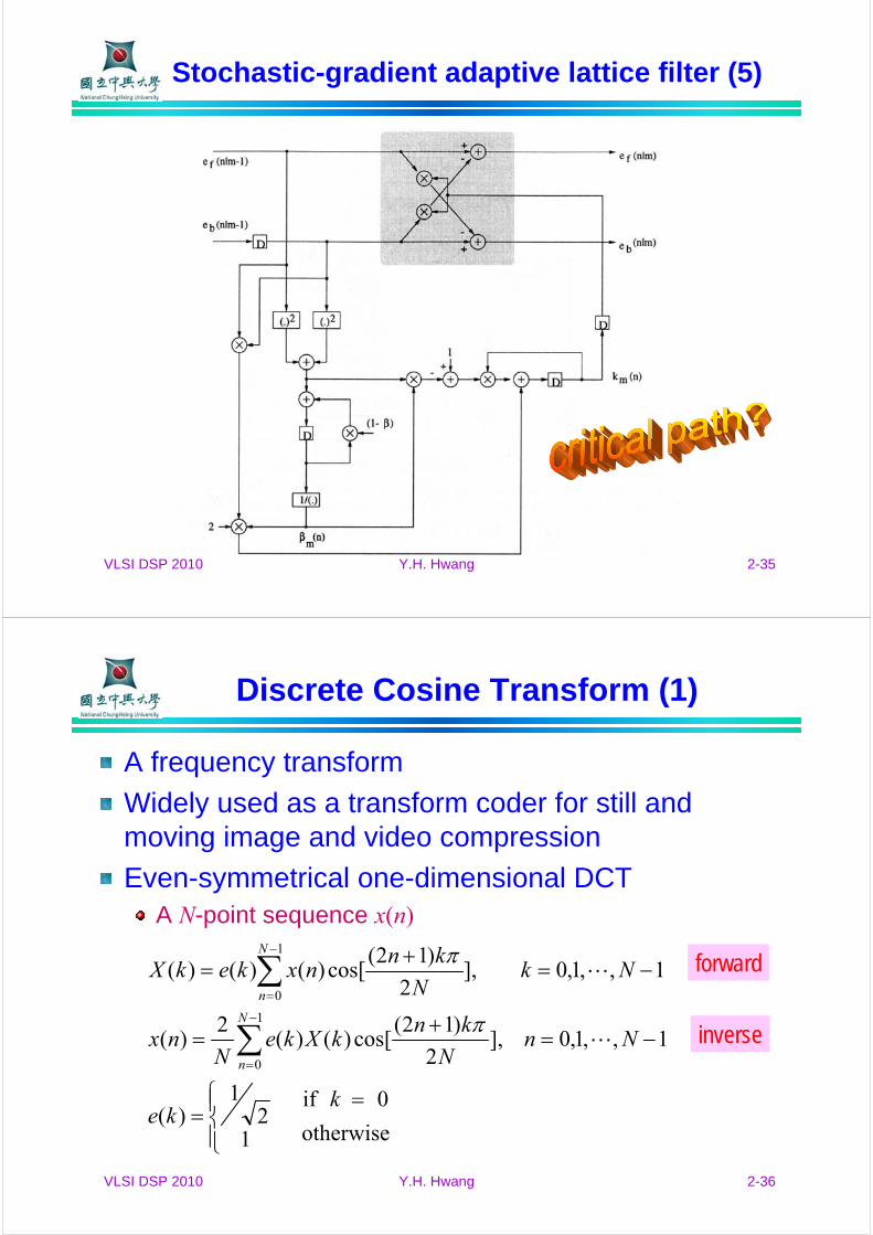
Stochastic-gradient adaptive lattice filter (4)
Stochastic-gradient adaptive algorithm
)1|()()1|1()|(
)1|1()()1|()|(
)1|(
1
)1|1()1|(
)1|()1()1|1(
)1|1()1|()(2
))]1|1()1|()((1)[()1(
22
22
−−−−=
−−−−=−
=
−−+−+
−−=−+
−−−+
−−+−−=+
mnenkmnemne
mnenkmnemne
mnSβ
mnemne
mnSmnS
mnemnen
mnemnennknk
fmbb
bmff
m
bf
bfm
bfmmm
β
β
β
Adaptation equations
Order-update equations
VLSI DSP 2010 Y.H. Hwang 2-35
Stochastic-gradient adaptive lattice filter (5)
VLSI DSP 2010 Y.H. Hwang 2-36
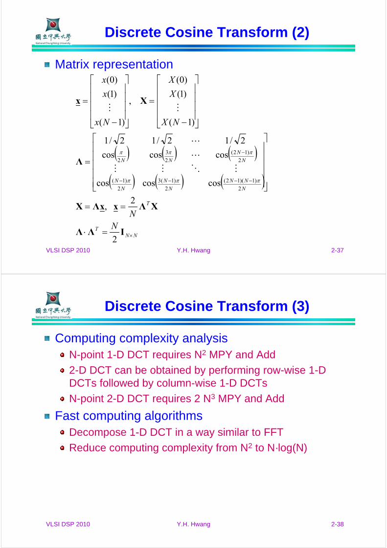
Discrete Cosine Transform (1)
A frequency transform
Widely used as a transform coder for still and moving image and video compression
Even-symmetrical one-dimensional DCTA N-point sequence x(n)
otherwise
0 if
12
1)(
1,,1,0 ],2
)12(cos[)()(
2)(
1,,1,0 ],2
)12(cos[)()()(
1
0
1
0
k ke
NnN
knkXke
Nnx
NkN
knnxkekX
N
n
N
n
=
⎪⎩
⎪⎨⎧
=
−=+
=
−=+
=
∑
∑−
=
−
=
π
π forward
inverse
VLSI DSP 2010 Y.H. Hwang 2-37
Discrete Cosine Transform (2)
Matrix representation
( ) ( ) ( )
( ) ( ) ( )
NNT
T
N
NN
N
N
N
N
N
N
NN
NN
NX
X
X
Nx
x
x
×
−−−−
−
=⋅
==
⎥⎥⎥⎥⎥
⎦
⎤
⎢⎢⎢⎢⎢
⎣
⎡
=
⎥⎥⎥⎥
⎦
⎤
⎢⎢⎢⎢
⎣
⎡
−
=
⎥⎥⎥⎥
⎦
⎤
⎢⎢⎢⎢
⎣
⎡
−
=
IΛΛ
XΛxxΛX
Λ
Xx
2
2 ,
coscoscos
coscoscos
2/12/12/1
)1(
)1(
)0(
,
)1(
)1(
)0(
2
)1)(12(
2
)1(3
2
)1(
2
)12(
2
3
2
πππ
πππ
VLSI DSP 2010 Y.H. Hwang 2-38
Discrete Cosine Transform (3)
Computing complexity analysisN-point 1-D DCT requires N2 MPY and Add
2-D DCT can be obtained by performing row-wise 1-D DCTs followed by column-wise 1-D DCTs
N-point 2-D DCT requires 2 N3 MPY and Add
Fast computing algorithmsDecompose 1-D DCT in a way similar to FFT
Reduce computing complexity from N2 to N·log(N)
VLSI DSP 2010 Y.H. Hwang 2-39
Wavelets and Filter Banks (1)
BasicsApplications: speech and image compression
Signals are represented using a set of basis functions (wavelets)
Derived by shifting and scaling wavelets in time
Decomposition of a signal in the time-scale (frequency) plane
Can be regarded as a multi-resolution sub-band filtering
VLSI DSP 2010 Y.H. Hwang 2-40
Wavelets and Filter Banks (2)
1-D DWT
h (n): mother wavelets
hi(2i+1n-k): basis functions (scaled and shifted versions of mother wavelets)
1-D IDWT
∑
∑∞
−∞=
−−−
∞
−∞=
+
−=−=
−≤≤−=
k
mmm
k
iii
miknhkxny
miknhkxny
1for ),2()()(
20for ),2()()(
111
1
basis functions
Wavelet coefficients
∑
∑∑∞
−∞=
−−−
−
=
∞
−∞=
+
−+
−=
k
mmm
m
i k
iii
knfky
knfkynx
)2()(
)2()()(
111
2
0
1
VLSI DSP 2010 Y.H. Hwang 2-41
Wavelets and Filter Banks (3)
Example for decomposition level m = 4computations are similar to convolution operations
digital filter banks with a common input x(k)
∑
∑
∑
∑
∞
−∞=
∞
−∞=
∞
−∞=
∞
−∞=
−=
−=
−=
−=
k
k
k
k
knhkxy
knhkxy
knhkxy
knhkxy
)8()(
)8()(
)4()(
)2()(
33
22
11
00
VLSI DSP 2010 Y.H. Hwang 2-42
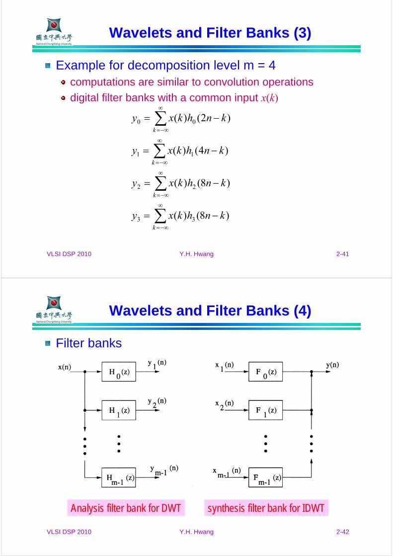
Wavelets and Filter Banks (4)
Filter banks
Analysis filter bank for DWT synthesis filter bank for IDWT
VLSI DSP 2010 Y.H. Hwang 2-43
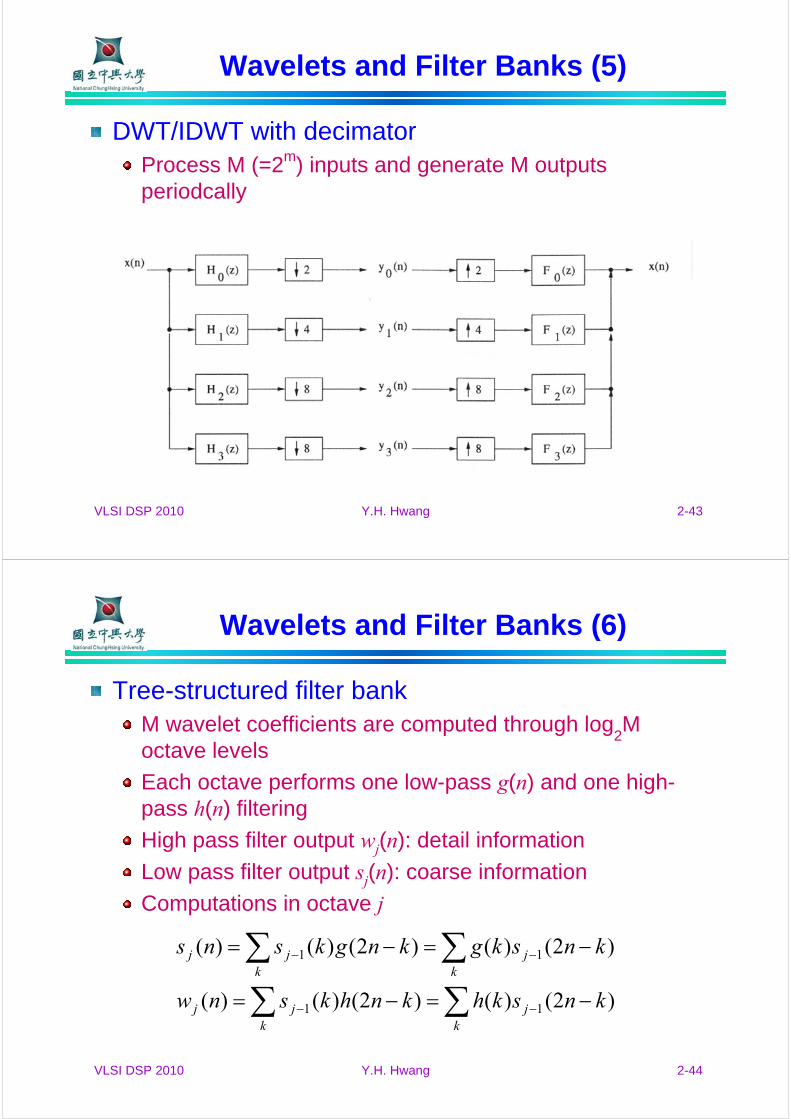
Wavelets and Filter Banks (5)
DWT/IDWT with decimatorProcess M (=2m) inputs and generate M outputs periodcally
VLSI DSP 2010 Y.H. Hwang 2-44
Wavelets and Filter Banks (6)
Tree-structured filter bankM wavelet coefficients are computed through log
2M
octave levels
Each octave performs one low-pass g(n) and one high-pass h(n) filtering
High pass filter output wj(n): detail information
Low pass filter output sj(n): coarse information
Computations in octave j
∑∑∑∑
−=−=
−=−=
−−
−−
kj
kjj
kj
kjj
knskhknhksnw
knskgkngksns
)2()()2()()(
)2()()2()()(
11
11
VLSI DSP 2010 Y.H. Hwang 2-45
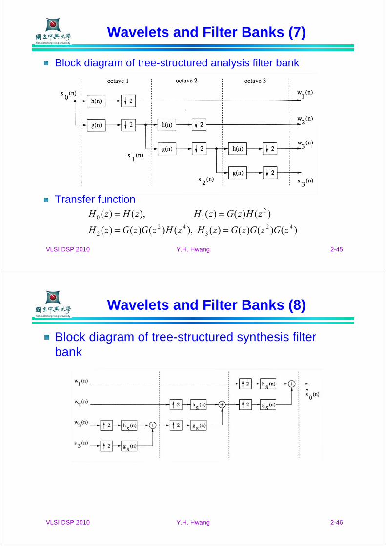
Wavelets and Filter Banks (7)
Block diagram of tree-structured analysis filter bank
Transfer function
)()()()( ),()()()(
)()()( ),()(42
342
2
210
zGzGzGzHzHzGzGzH
zHzGzHzHzH
==
==
VLSI DSP 2010 Y.H. Hwang 2-46
Wavelets and Filter Banks (8)
Block diagram of tree-structured synthesis filter bank
VLSI DSP 2010 Y.H. Hwang 2-47
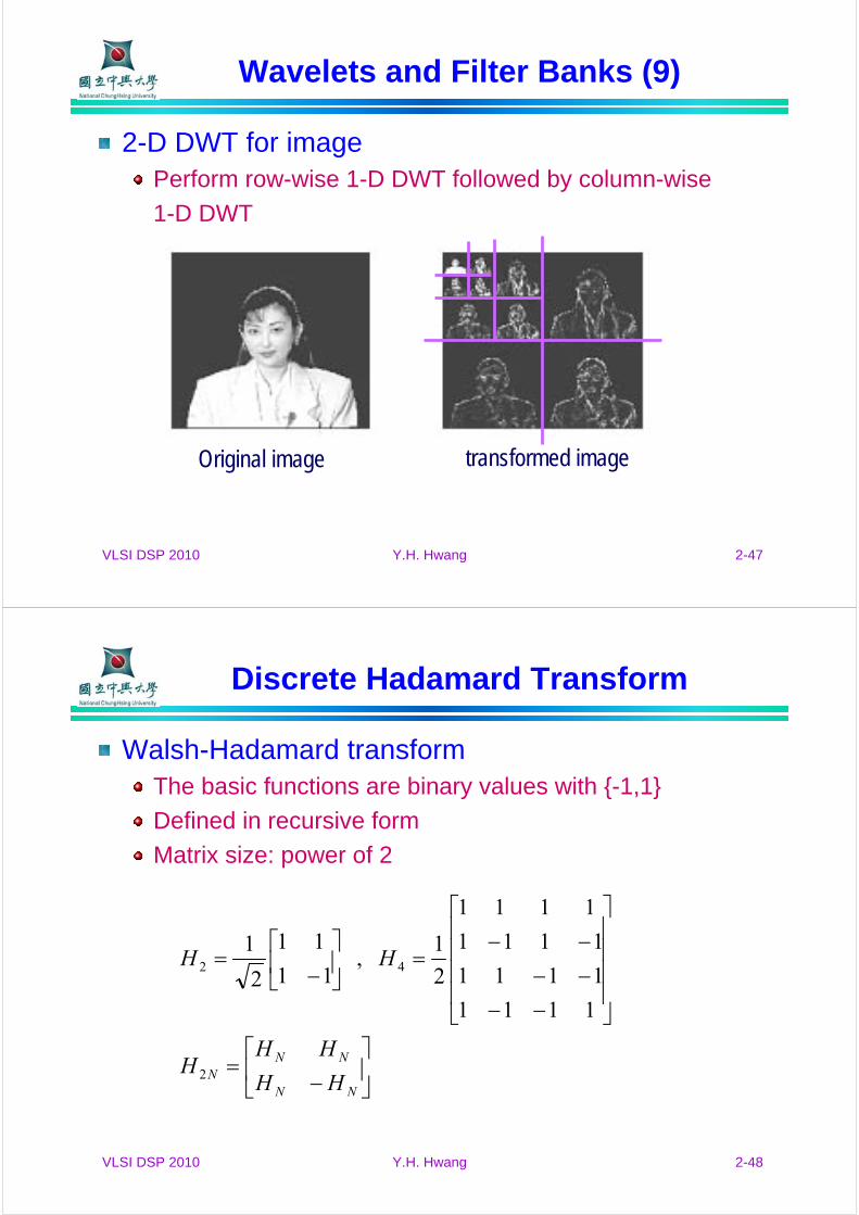
Wavelets and Filter Banks (9)
2-D DWT for imagePerform row-wise 1-D DWT followed by column-wise
1-D DWT
Original image transformed image
VLSI DSP 2010 Y.H. Hwang 2-48
⎥⎦
⎤⎢⎣
⎡−
=
⎥⎥⎥⎥
⎦
⎤
⎢⎢⎢⎢
⎣
⎡
−−−−−−
=⎥⎦
⎤⎢⎣
⎡−
=
NN
NNN HH
HHH
HH
2
42
1111
1111
1111
1111
2
1,
11
11
2
1
Discrete Hadamard Transform
Walsh-Hadamard transformThe basic functions are binary values with {-1,1}
Defined in recursive form
Matrix size: power of 2
VLSI DSP 2010 Y.H. Hwang 2-49
{ }22,,1,0, where
),(),(),(
21
22110 0
2121
1
1
2
2
−⋅⋅⋅∈
−−⋅= ∑∑= =
Nnn
knknwkkunnyn
k
n
k
u( , )
N
N w ( , )N
N
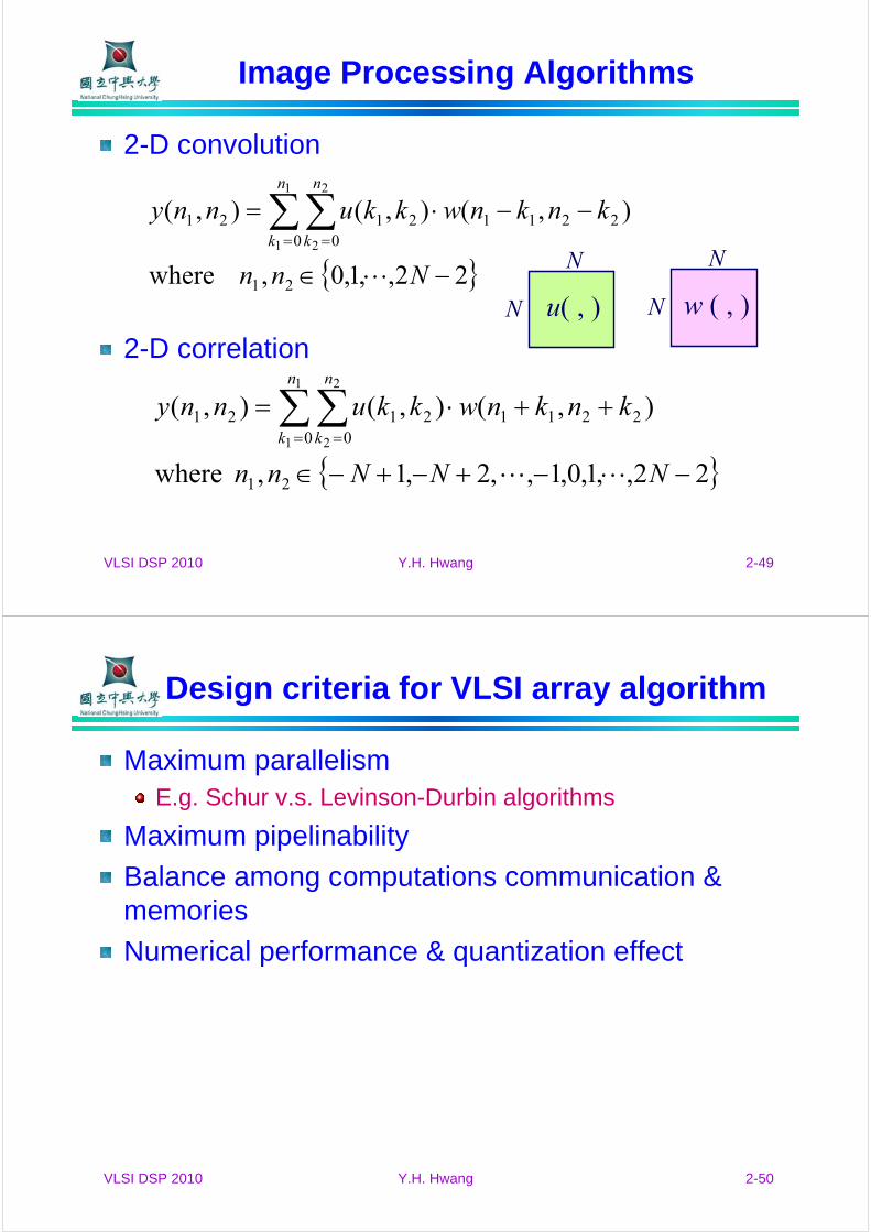
Image Processing Algorithms
2-D convolution
2-D correlation
{ }22,,1,0,1,,2,1, where
),(),(),(
21
22110 0
2121
1
1
2
2
−⋅⋅⋅−+−+−∈
++⋅= ∑∑= =
NNNnn
knknwkkunnyn
k
n
k
VLSI DSP 2010 Y.H. Hwang 2-50
Design criteria for VLSI array algorithm
Maximum parallelismE.g. Schur v.s. Levinson-Durbin algorithms
Maximum pipelinability
Balance among computations communication & memories
Numerical performance & quantization effect
VLSI DSP 2010 Y.H. Hwang 2-51
Part 2 Algorithm Representation
VLSI DSP 2010 Y.H. Hwang 2-52
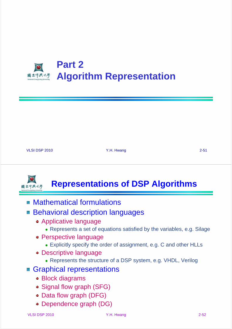
Representations of DSP Algorithms
Mathematical formulationsBehavioral description languages
Applicative languageRepresents a set of equations satisfied by the variables, e.g. Silage
Perspective languageExplicitly specify the order of assignment, e.g. C and other HLLs
Descriptive languageRepresents the structure of a DSP system, e.g. VHDL, Verilog
Graphical representationsBlock diagramsSignal flow graph (SFG)Data flow graph (DFG)Dependence graph (DG)
VLSI DSP 2010 Y.H. Hwang 2-53
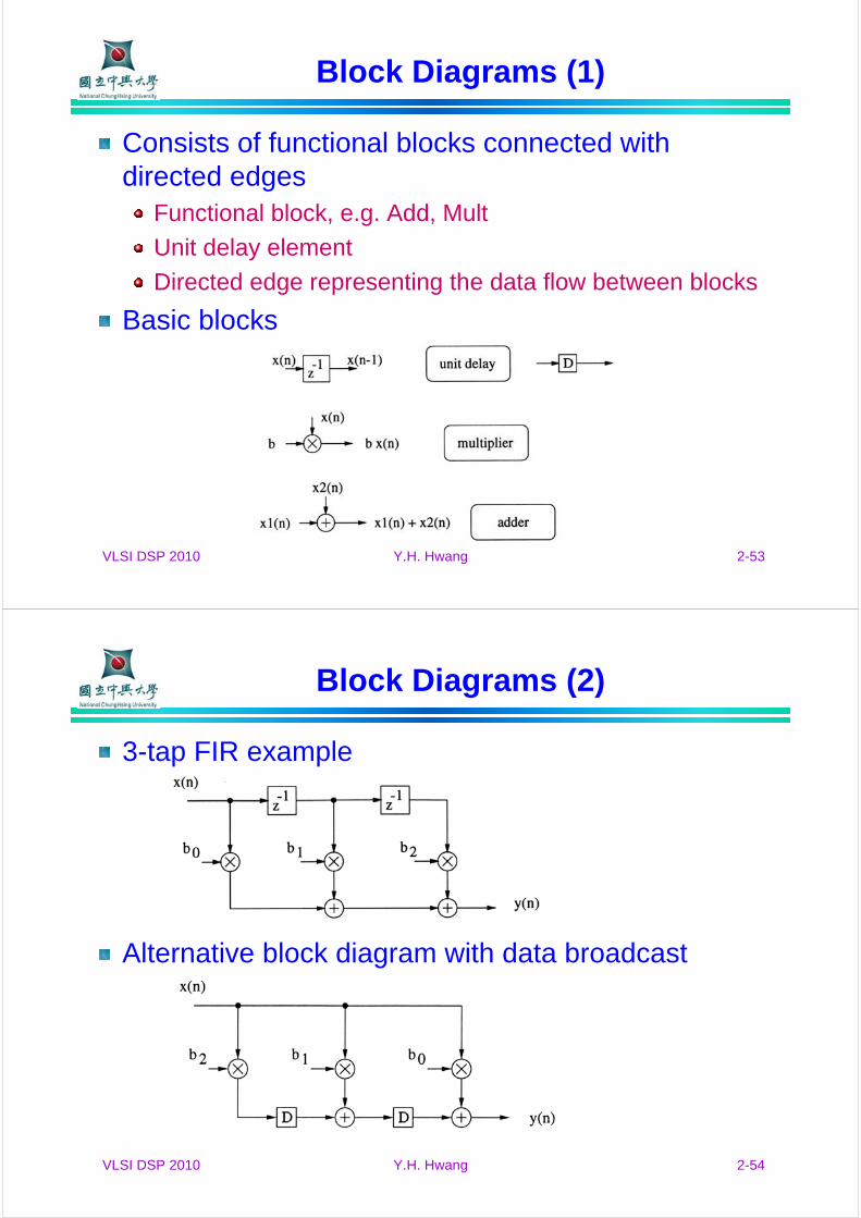
Block Diagrams (1)
Consists of functional blocks connected with directed edges
Functional block, e.g. Add, Mult
Unit delay element
Directed edge representing the data flow between blocks
Basic blocks
VLSI DSP 2010 Y.H. Hwang 2-54
Block Diagrams (2)
3-tap FIR example
Alternative block diagram with data broadcast
VLSI DSP 2010 Y.H. Hwang 2-55
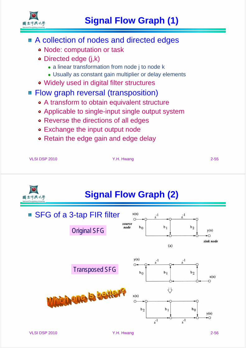
Signal Flow Graph (1)
A collection of nodes and directed edgesNode: computation or taskDirected edge (j,k)
a linear transformation from node j to node kUsually as constant gain multiplier or delay elements
Widely used in digital filter structures
Flow graph reversal (transposition)A transform to obtain equivalent structureApplicable to single-input single output systemReverse the directions of all edgesExchange the input output nodeRetain the edge gain and edge delay
VLSI DSP 2010 Y.H. Hwang 2-56
Signal Flow Graph (2)
SFG of a 3-tap FIR filter
Original SFG
Transposed SFG

VLSI DSP 2010 Y.H. Hwang 2-57
Signal Flow Graph (3)
Limitations of transpositioncan be applied to MIMO systems described by symmetric transform matrices
More on SFGApplicable to linear network
Cannot be used to described multi-rate system
VLSI DSP 2010 Y.H. Hwang 2-58
Data Flow Graph (1)
DFGNode: computation (function or subtask)
Directed edge: data path or communication between nodes
Associated edge delay: non-negative
Associated node delay: execution time of each node
Block diagram Conventional DFG Synchronous DFG
add
mpy
VLSI DSP 2010 Y.H. Hwang 2-59
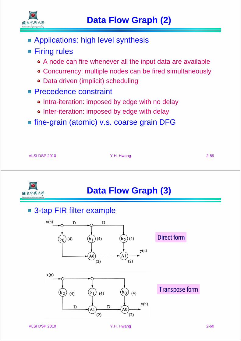
Data Flow Graph (2)
Applications: high level synthesis
Firing rulesA node can fire whenever all the input data are available
Concurrency: multiple nodes can be fired simultaneously
Data driven (implicit) scheduling
Precedence constraintIntra-iteration: imposed by edge with no delay
Inter-iteration: imposed by edge with delay
fine-grain (atomic) v.s. coarse grain DFG
VLSI DSP 2010 Y.H. Hwang 2-60
Data Flow Graph (3)
3-tap FIR filter example
Direct form
Transpose form
VLSI DSP 2010 Y.H. Hwang 2-61
Data Flow Graph (4)
Synchronous DFGNumber of data samples produced or consumed by each node is specified a priori
Single rate system
Multi-rate system: different nodes working on different frequencies
Multi-rate system can be represented by a single rate system via unfolding (unrolling)
VLSI DSP 2010 Y.H. Hwang 2-62
Part 3 Part 3 Iteration BoundIteration Bound
VLSI DSP 2010 Y.H. Hwang 2-63
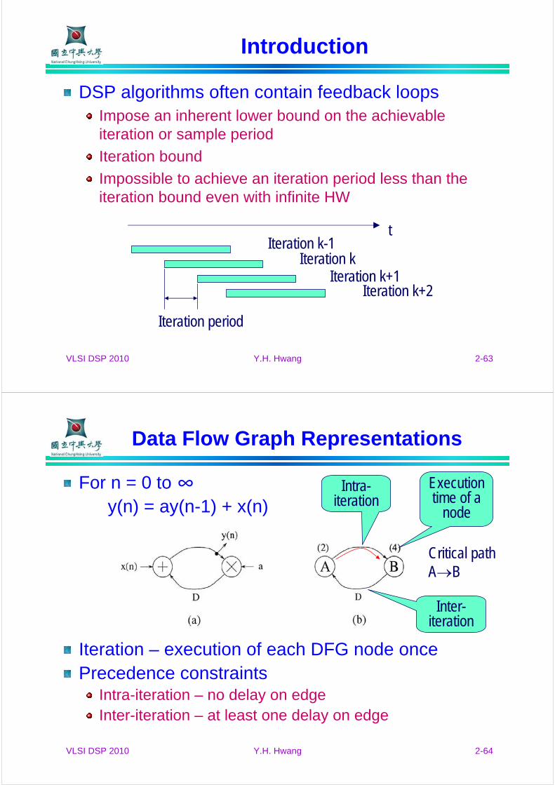
Introduction
DSP algorithms often contain feedback loopsImpose an inherent lower bound on the achievable iteration or sample period
Iteration bound
Impossible to achieve an iteration period less than the iteration bound even with infinite HW
Iteration kIteration k-1
Iteration k+1Iteration k+2
t
Iteration period
VLSI DSP 2010 Y.H. Hwang 2-64
Data Flow Graph Representations
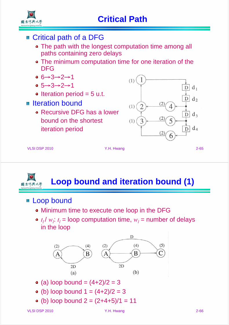
For n = 0 to ∞y(n) = ay(n-1) + x(n)
Iteration – execution of each DFG node oncePrecedence constraints
Intra-iteration – no delay on edgeInter-iteration – at least one delay on edge
Execution time of a
node
Inter-iteration
Intra-iteration
Critical pathA→B
VLSI DSP 2010 Y.H. Hwang 2-65
Critical Path
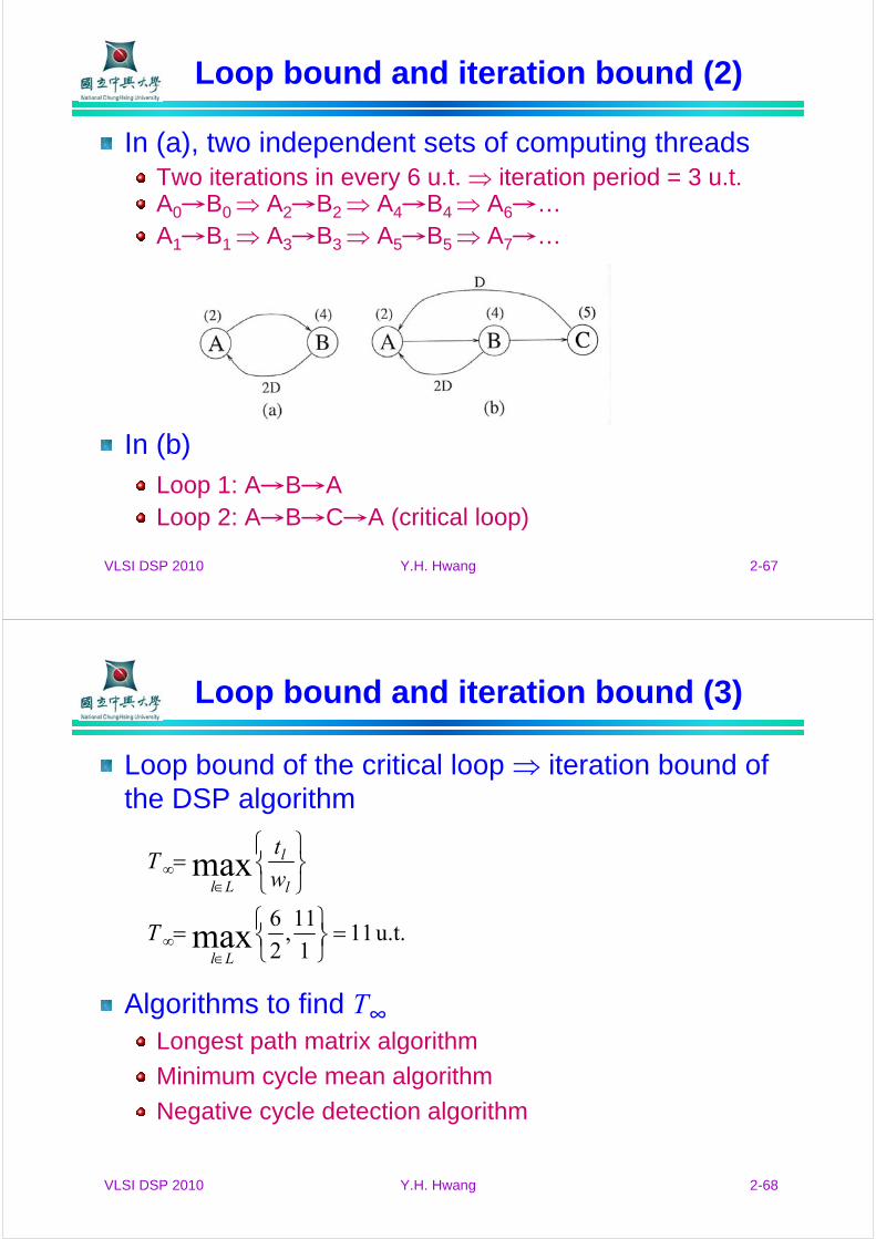
Critical path of a DFGThe path with the longest computation time among all paths containing zero delaysThe minimum computation time for one iteration of the DFG6→3→2→15→3→2→1Iteration period = 5 u.t.
Iteration boundRecursive DFG has a lowerbound on the shortestiteration period
VLSI DSP 2010 Y.H. Hwang 2-66
Loop bound and iteration bound (1)
Loop boundMinimum time to execute one loop in the DFG
tl / wl: tl = loop computation time, wl = number of delays in the loop
(a) loop bound = (4+2)/2 = 3
(b) loop bound 1 = (4+2)/2 = 3
(b) loop bound 2 = (2+4+5)/1 = 11
VLSI DSP 2010 Y.H. Hwang 2-67
Loop bound and iteration bound (2)
In (a), two independent sets of computing threadsTwo iterations in every 6 u.t. ⇒ iteration period = 3 u.t.A0→B0 ⇒ A2→B2 ⇒ A4→B4 ⇒ A6→…A1→B1 ⇒ A3→B3 ⇒ A5→B5 ⇒ A7→…
In (b)Loop 1: A→B→ALoop 2: A→B→C→A (critical loop)
VLSI DSP 2010 Y.H. Hwang 2-68
Loop bound and iteration bound (3)
Loop bound of the critical loop ⇒ iteration bound of the DSP algorithm
Algorithms to find T∞Longest path matrix algorithm
Minimum cycle mean algorithm
Negative cycle detection algorithm
u.t. 111
11,
2
6max
max
=⎭⎬⎫
⎩⎨⎧=
⎭⎬⎫
⎩⎨⎧
=
∈∞
∈∞
Ll
l
l
Ll
T
w
tT
VLSI DSP 2010 Y.H. Hwang 2-69
Longest path matrix (LPM) algorithm (1)
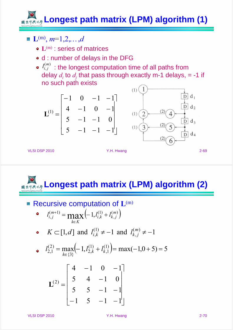
L(m), m=1,2,…,dL(m) : series of matrices
d : number of delays in the DFG
: the longest computation time of all paths from delay di to dj that pass through exactly m-1 delays, = -1 if no such path exists
)(,mjil
⎥⎥⎥⎥
⎦
⎤
⎢⎢⎢⎢
⎣
⎡
−−−−−
−−−−−
=
1115
0115
1014
1101
)1(L
VLSI DSP 2010 Y.H. Hwang 2-70
Longest path matrix (LPM) algorithm (2)
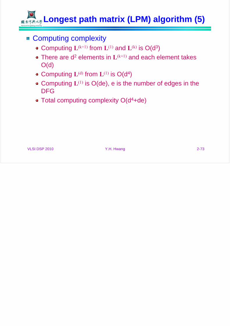
Recursive computation of L(m)
( ))(,
)1(,
)1(, ,1max m
jkkiKk
mji lll +−=
∈
+
1 and 1 and ],1[ )(,
)1(, −≠−≠⊂ m
jkki lldK
( ) 5)50,1max(,1max )1(1,
)1(,2
}3{
)2(1,2 =+−=+−=
∈kk
klll
⎥⎥⎥⎥
⎦
⎤
⎢⎢⎢⎢
⎣
⎡
−−−−−
−−−
=
1151
1155
0145
1014
)2(L

VLSI DSP 2010 Y.H. Hwang 2-71
Longest path matrix (LPM) algorithm (3)
Computing L(3) using L(1) and L(2)
Iteration bound
( ) 5)05,1max(,1max )2(3,
)1(,3
}1{
)3(3,3 =+−=+−=
∈kk
klll
⎥⎥⎥⎥
⎦
⎤
⎢⎢⎢⎢
⎣
⎡
−
−
=
⎥⎥⎥⎥
⎦
⎤
⎢⎢⎢⎢
⎣
⎡
−−−−
−
=
51910
55910
4589
1458
1519
1559
1458
0145
)4()3( LL
24
5,
4
5,
4
8,
4
8,
3
5,
3
5,
3
5,
2
4,
2
4max
max)(
,
},,2,1{,
=⎭⎬⎫
⎩⎨⎧=
⎪⎭
⎪⎬⎫
⎪⎩
⎪⎨⎧
=∈
∞ m
lT
mii
dmi
VLSI DSP 2010 Y.H. Hwang 2-72
Longest path matrix (LPM) algorithm (4)
the longest computation time of all loops with m delays and containing delay element di
Another example
82
16,
2
12,
1
8,
1
4max
1616
1212
88
44
)2(
)1(
=⎭⎬⎫
⎩⎨⎧=
⎥⎦
⎤⎢⎣
⎡=
⎥⎦
⎤⎢⎣
⎡=
∞T
L
L
)(,miil
VLSI DSP 2010 Y.H. Hwang 2-73
Longest path matrix (LPM) algorithm (5)
Computing complexityComputing L(k+1) from L(1) and L(k) is O(d3)
There are d2 elements in L(k+1) and each element takes O(d)
Computing L(d) from L(1) is O(d4)
Computing L(1) is O(de), e is the number of edges in the DFG
Total computing complexity O(d4+de)
Related Documents
![Digital Signal Processing: Principles, Algorithms ...Title Digital Signal Processing: Principles, Algorithms & Applications (3rd Ed.) [ripped by sabbanji] Created Date 4/4/2010 9:50:12](https://static.cupdf.com/doc/110x72/612a06b8c03ce1685f3b1590/digital-signal-processing-principles-algorithms-title-digital-signal-processing.jpg)