Chapter 18,19

Chapter 18,19.

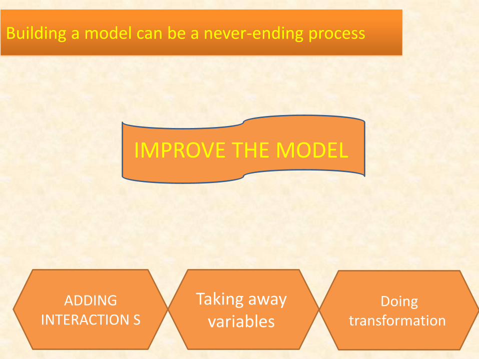
Building a model can be a never-ending process

IMPROVE THE MODEL

ADDING INTERACTION S

Taking away variables

Doing transformation

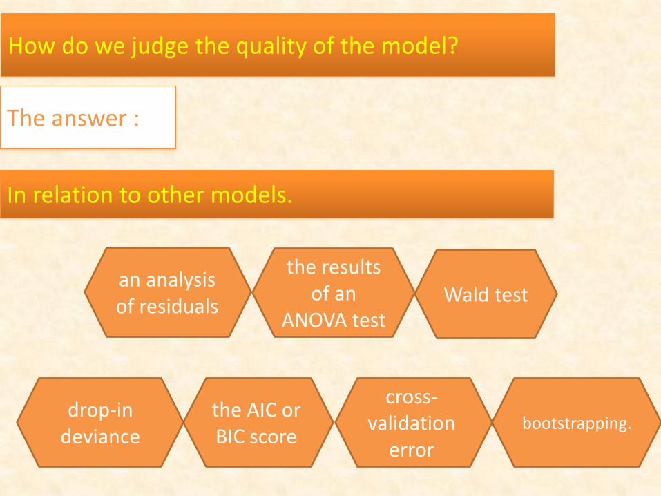
How do we judge the quality of the model?

The answer :

In relation to other models.

an analysis of residuals

drop-in deviance

the results of an

ANOVA test Wald test

the AIC or BIC score

cross-validation

error

bootstrapping.

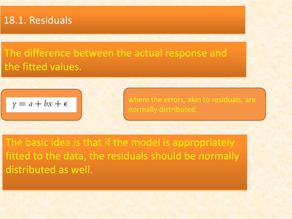
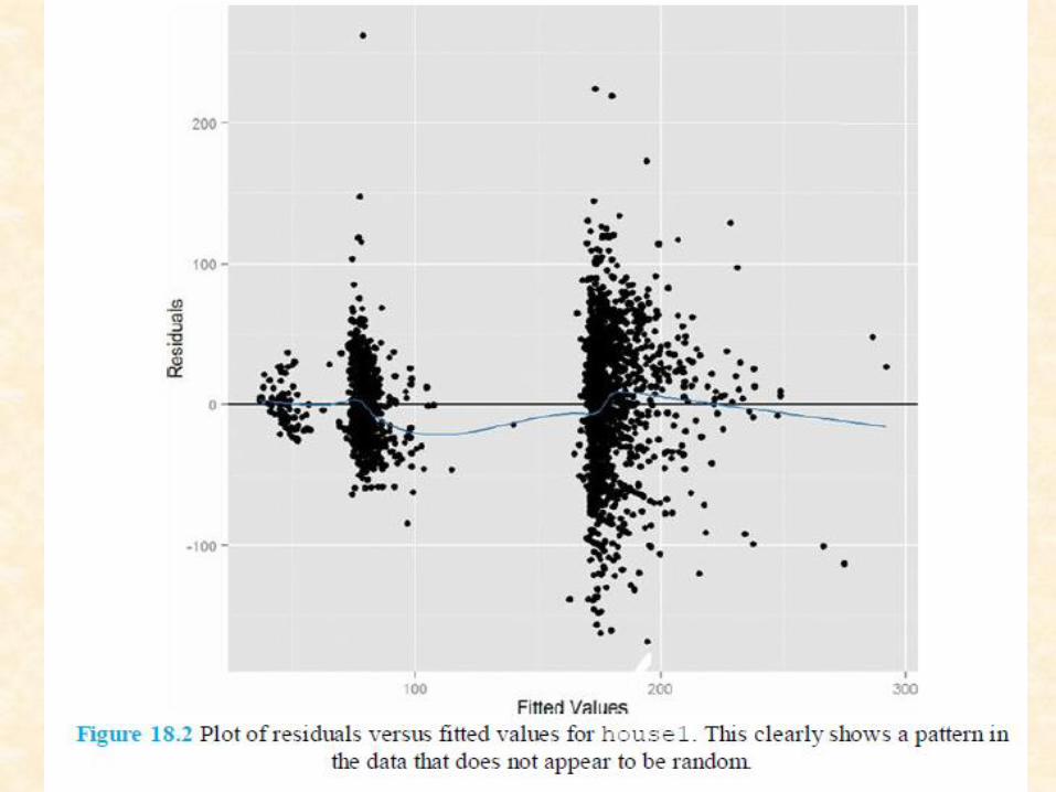
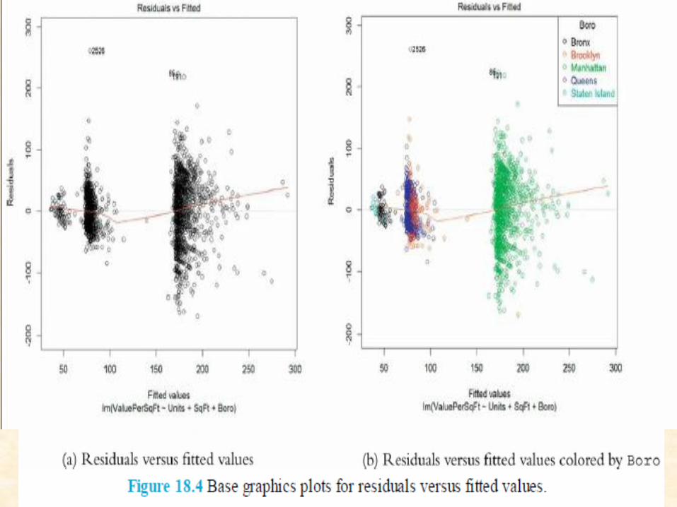
18.1. Residuals

The difference between the actual response and the fitted values.

where the errors, akin to residuals, are

normally distributed.

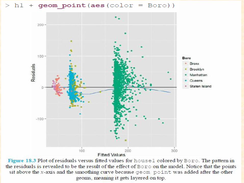
The basic idea is that if the model is appropriately fitted to the data, the residuals should be normally distributed as well.

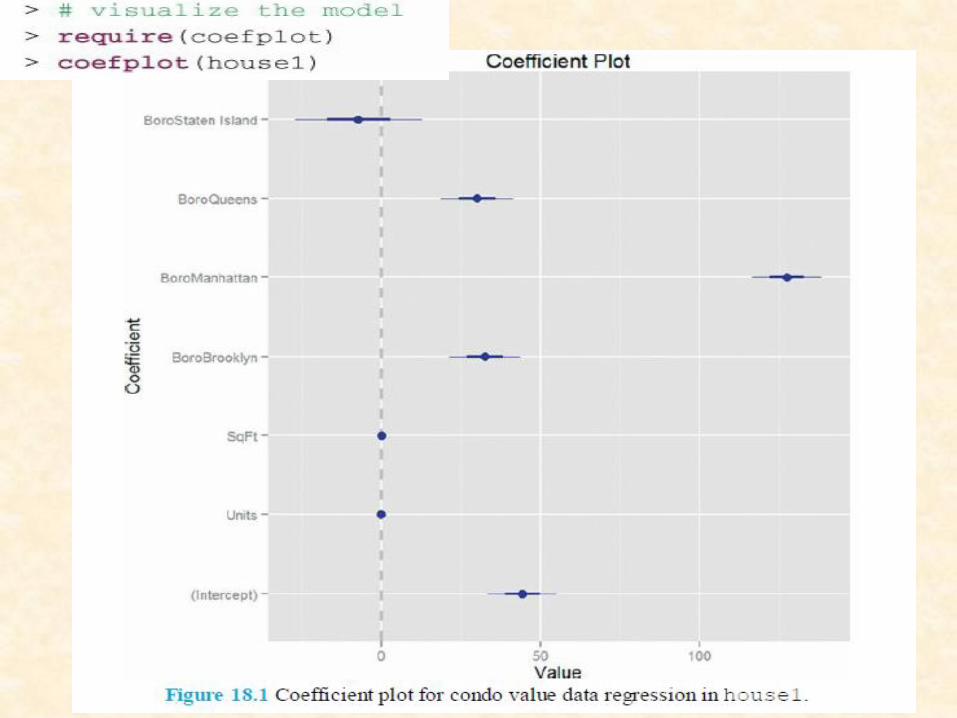
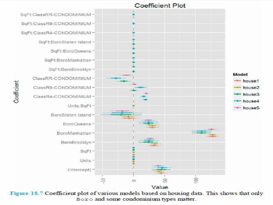
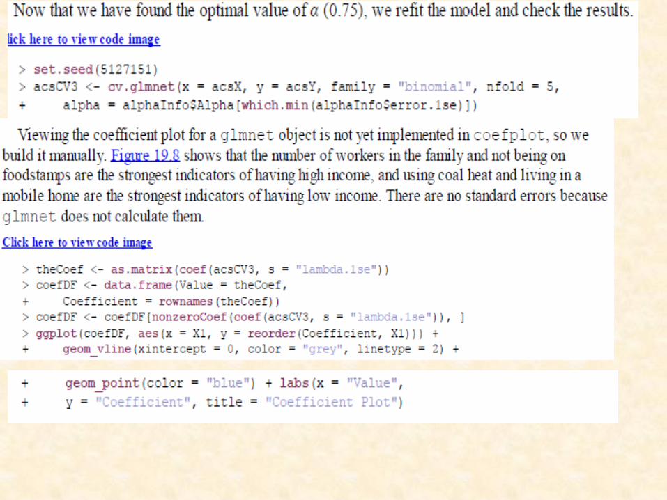
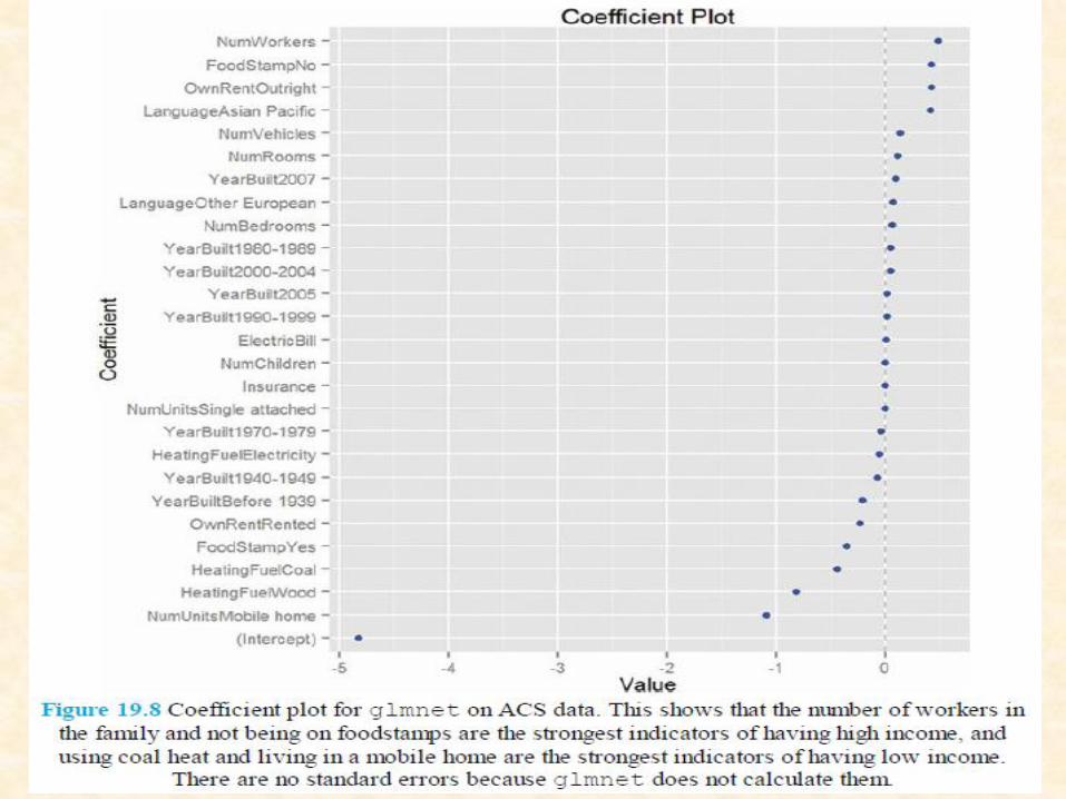
each coefficient is plotted as a point with a thick line representing the one standard error confidence interval and a thin line representing the two standard error confidence interval. There is a vertical line indicating 0. In general, a good rule of thumb is that if the two standard error confidence interval does not contain 0, it is statistically significant.

Remember

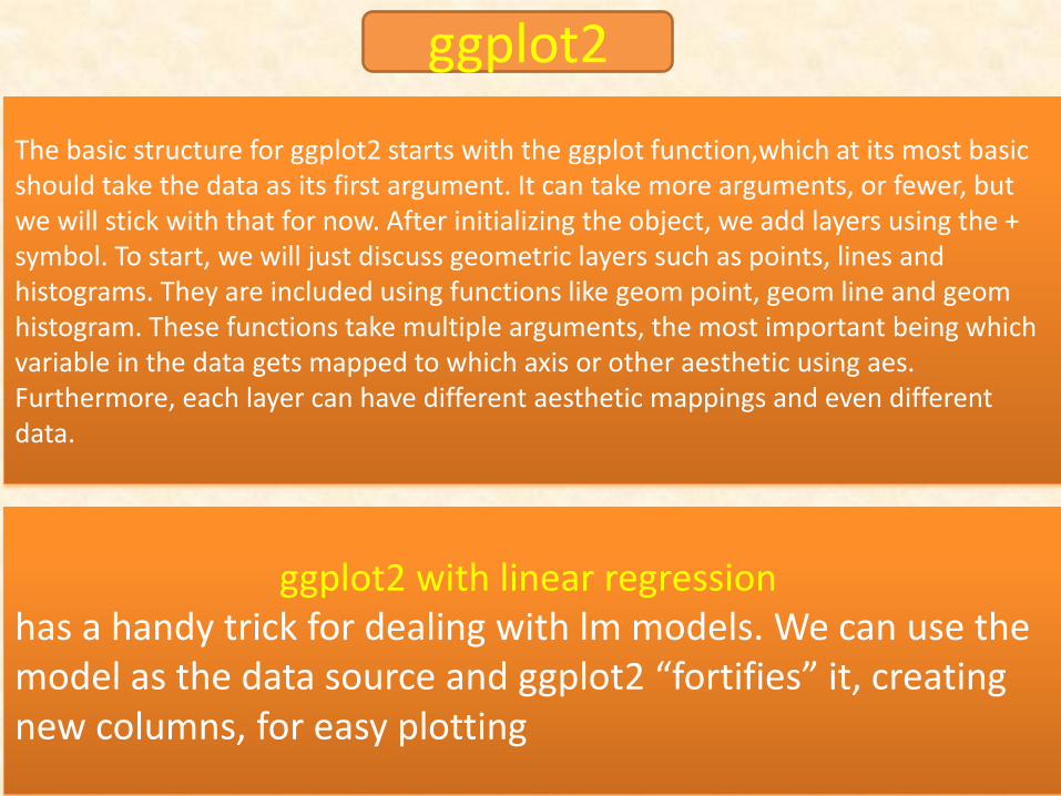
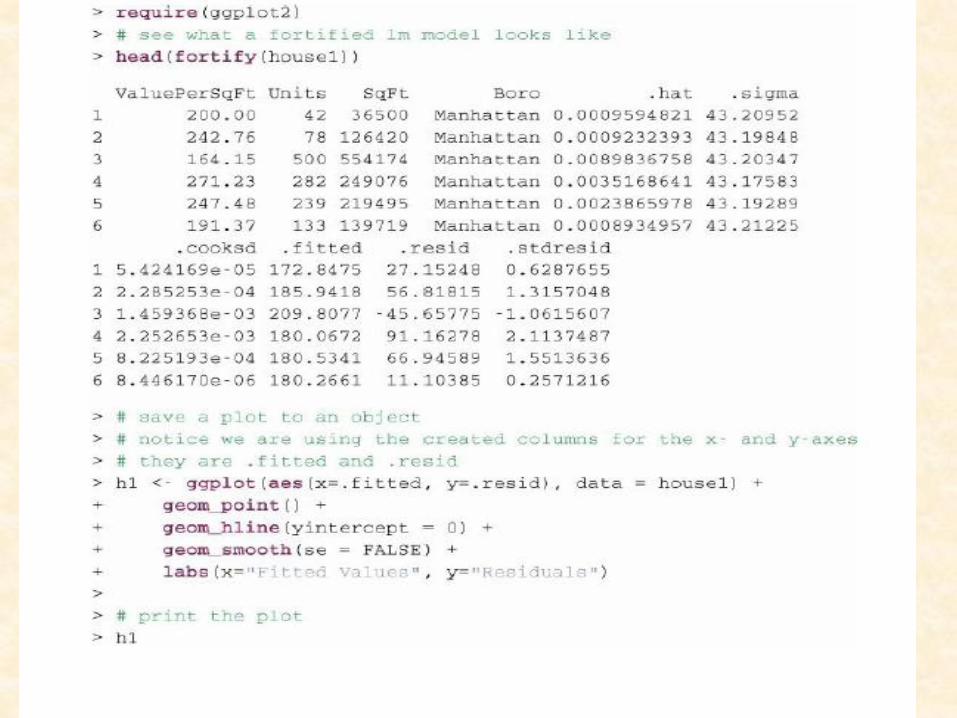
ggplot2 with linear regression

has a handy trick for dealing with lm models. We can use the model as the data source and ggplot2 “fortifies” it, creating new columns, for easy plotting

The basic structure for ggplot2 starts with the ggplot function,which at its most basic should take the data as its first argument. It can take more arguments, or fewer, but we will stick with that for now. After initializing the object, we add layers using the + symbol. To start, we will just discuss geometric layers such as points, lines and histograms. They are included using functions like geom point, geom line and geom histogram. These functions take multiple arguments, the most important being which variable in the data gets mapped to which axis or other aesthetic using aes. Furthermore, each layer can have different aesthetic mappings and even different data.

ggplot2

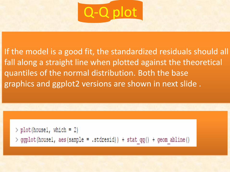
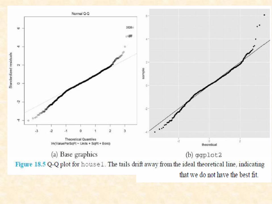
Q-Q plot

If the model is a good fit, the standardized residuals should all fall along a straight line when plotted against the theoretical quantiles of the normal distribution. Both the base graphics and ggplot2 versions are shown in next slide .

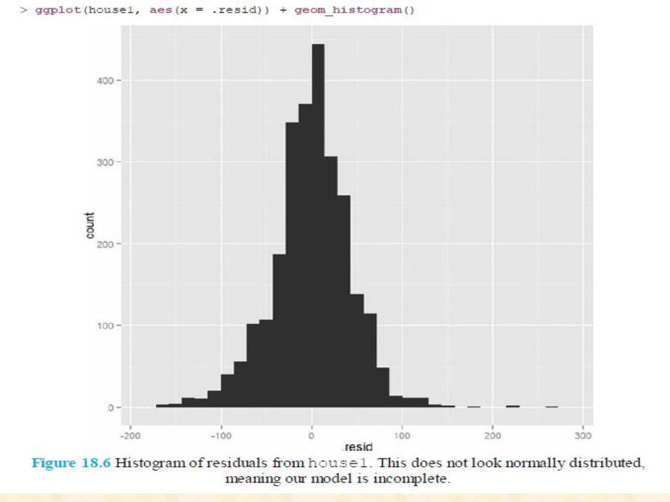
histogram of the residuals. This time we will not be showing the base graphics alternative because a histogram is standard plot that we have shown repeatedly. The histogram is not normally distributed, meaning model is not an entirely correct.

histogram

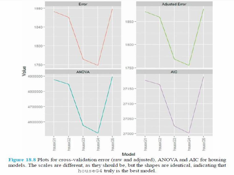
All of this measuring of model fit only really makes sense when comparing multiple models, because all of these measures are relative.

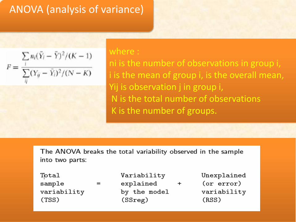
where : ni is the number of observations in group i, i is the mean of group i, is the overall mean, Yij is observation j in group i, N is the total number of observations K is the number of groups.

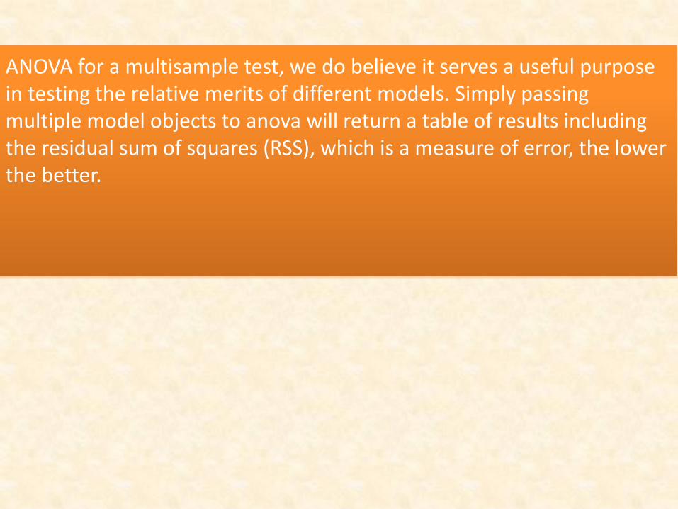
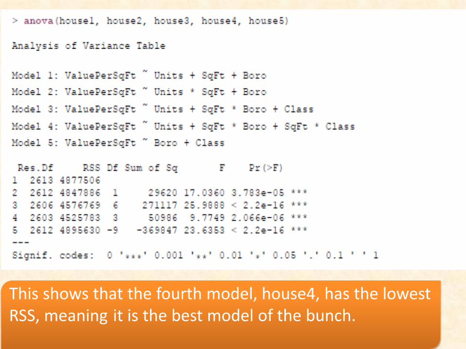
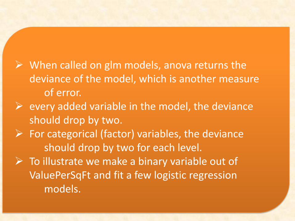
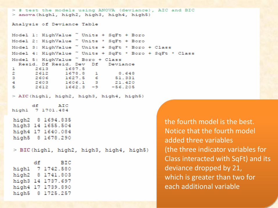
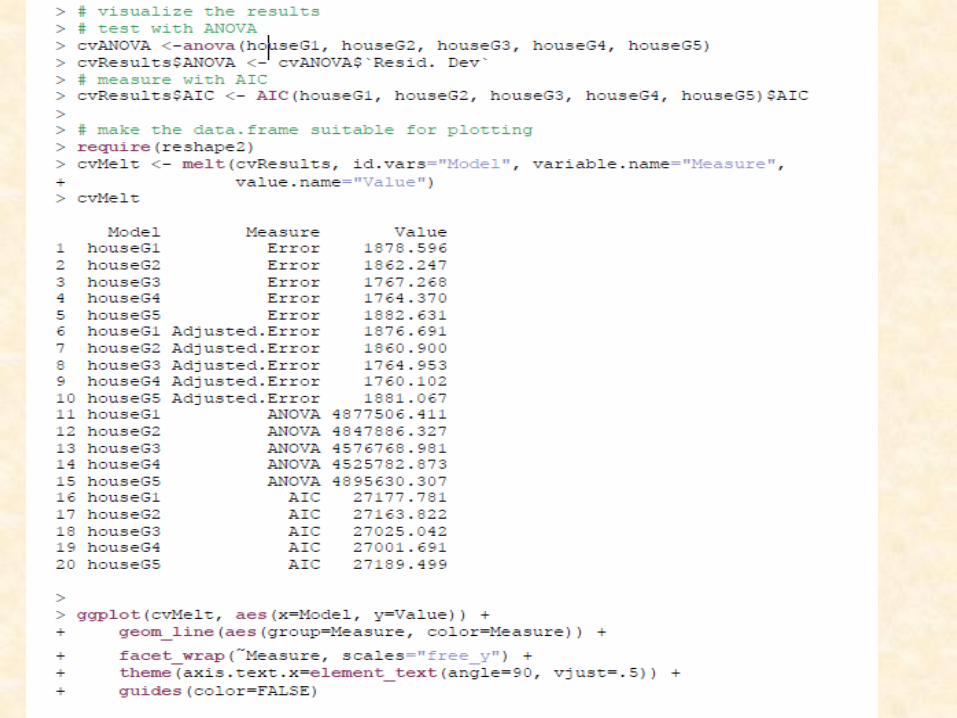
ANOVA for a multisample test, we do believe it serves a useful purpose in testing the relative merits of different models. Simply passing multiple model objects to anova will return a table of results including the residual sum of squares (RSS), which is a measure of error, the lower the better.

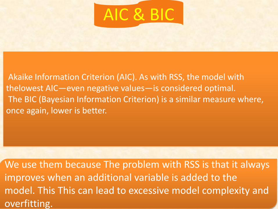
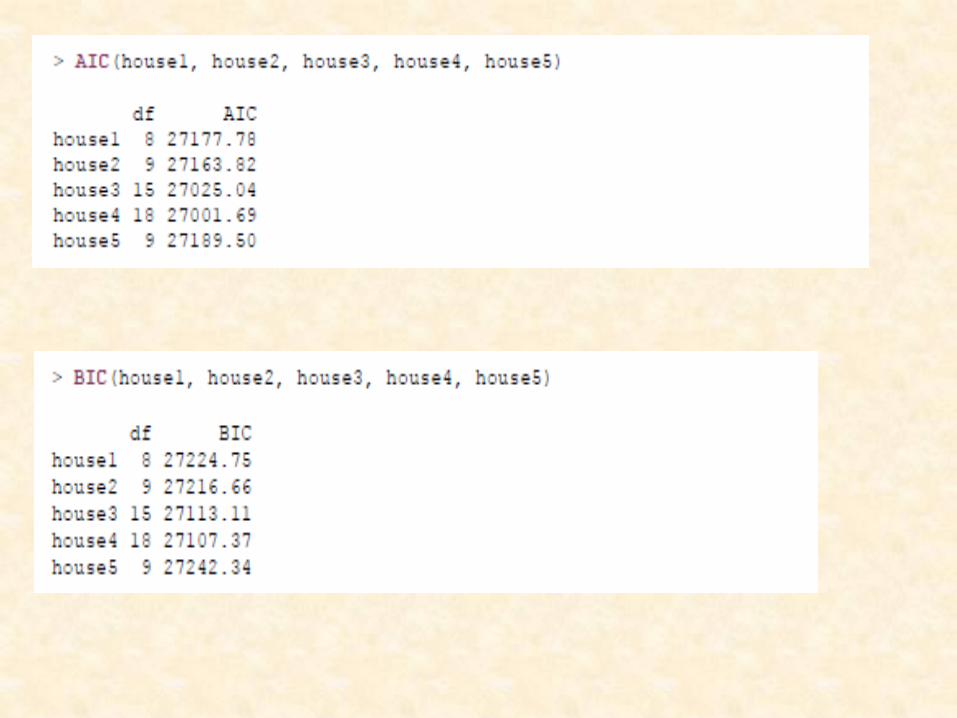
Akaike Information Criterion (AIC). As with RSS, the model with thelowest AIC—even negative values—is considered optimal. The BIC (Bayesian Information Criterion) is a similar measure where, once again, lower is better.

AIC & BIC

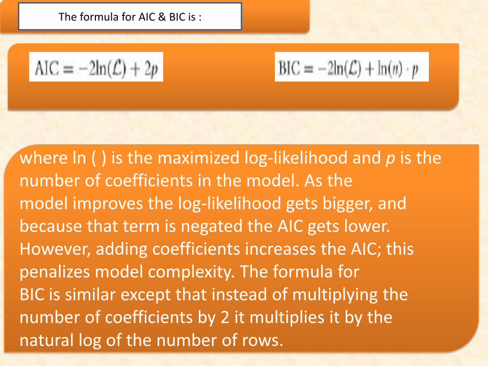
The formula for AIC & BIC is :

Cross-Validation

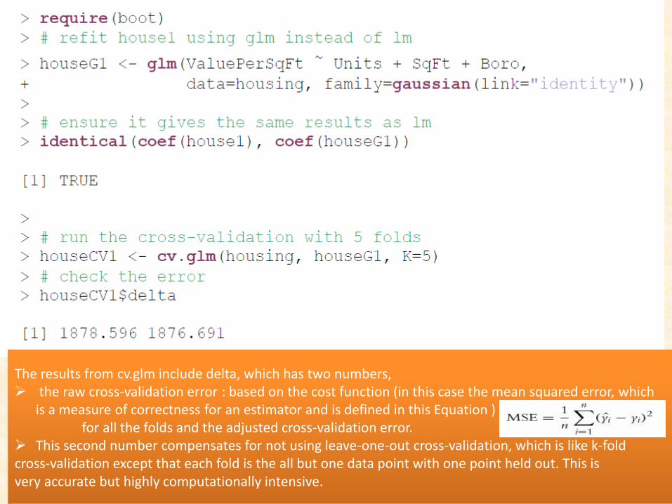
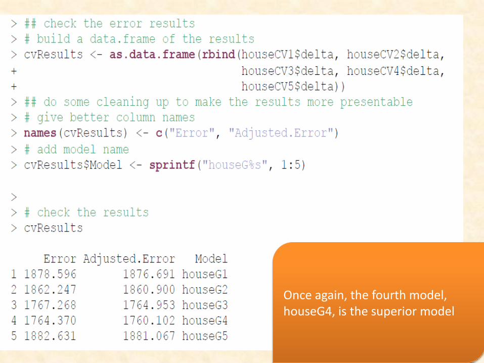
The results from cv.glm include delta, which has two numbers, the raw cross-validation error : based on the cost function (in this case the mean squared error, which

is a measure of correctness for an estimator and is defined in this Equation ) for all the folds and the adjusted cross-validation error. This second number compensates for not using leave-one-out cross-validation, which is like k-fold cross-validation except that each fold is the all but one data point with one point held out. This is very accurate but highly computationally intensive.

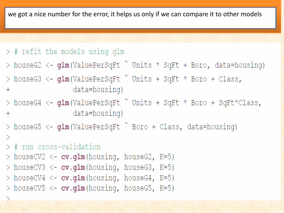
we got a nice number for the error, it helps us only if we can compare it to other models

Bootstrapping

The idea is that we start with n rows of data. Some statistic (whether a mean, regression or some arbitrary function) is applied to the data.

Then the data are sampled, creating a new dataset. This new set still has n rows except that there are repeats and other rows are

entirely missing. The statistic is applied to this new dataset. The process is repeated R times (typically around 1,200), which generates an

entire distribution for the statistic. This distribution can then be used to find the mean and confidence interval

(typically 95%) for the statistic. The boot package is a very robust set of tools for making the bootstrap easy to

compute

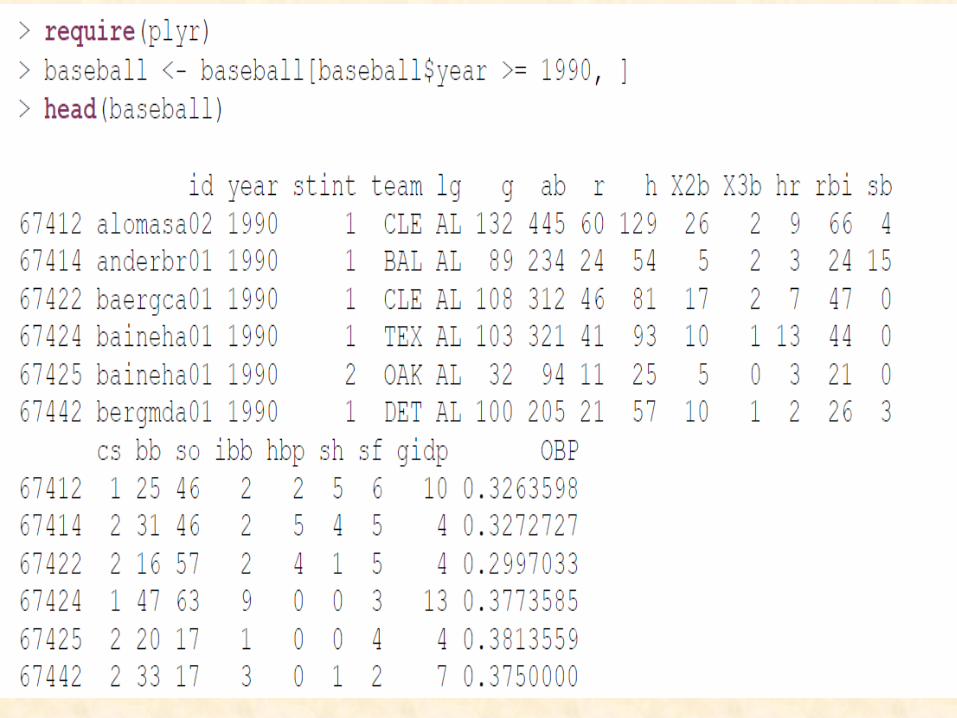
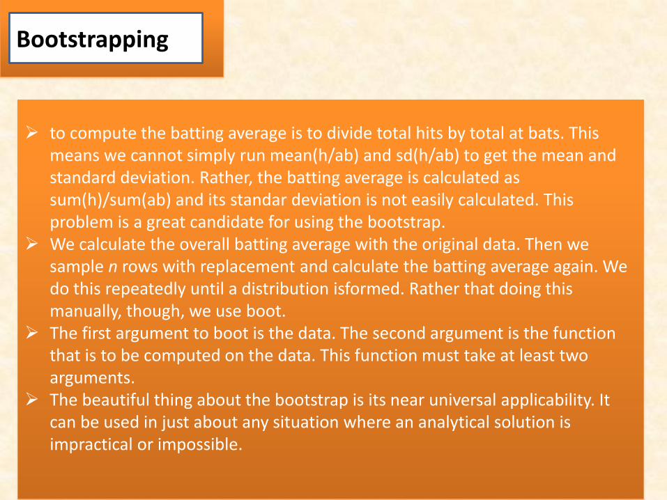
to compute the batting average is to divide total hits by total at bats. This means we cannot simply run mean(h/ab) and sd(h/ab) to get the mean and standard deviation. Rather, the batting average is calculated as sum(h)/sum(ab) and its standar deviation is not easily calculated. This problem is a great candidate for using the bootstrap.

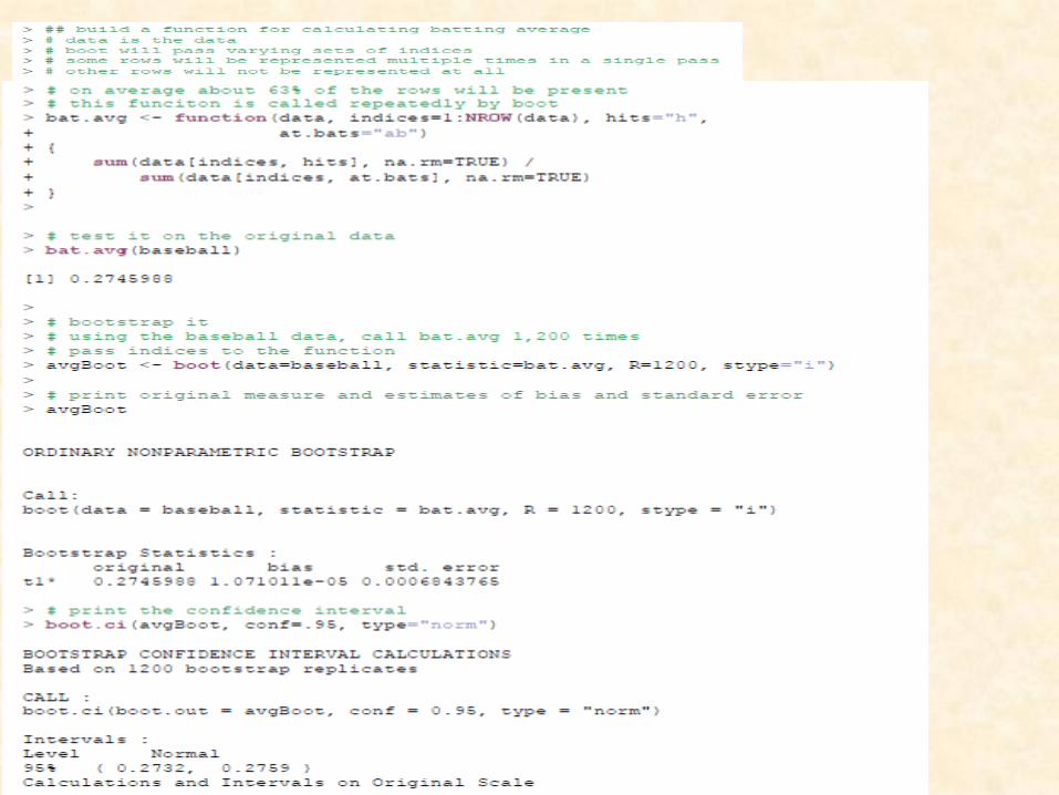
We calculate the overall batting average with the original data. Then we sample n rows with replacement and calculate the batting average again. We do this repeatedly until a distribution isformed. Rather that doing this manually, though, we use boot.

The first argument to boot is the data. The second argument is the function that is to be computed on the data. This function must take at least two arguments.

The beautiful thing about the bootstrap is its near universal applicability. It can be used in just about any situation where an analytical solution is impractical or impossible.

Bootstrapping

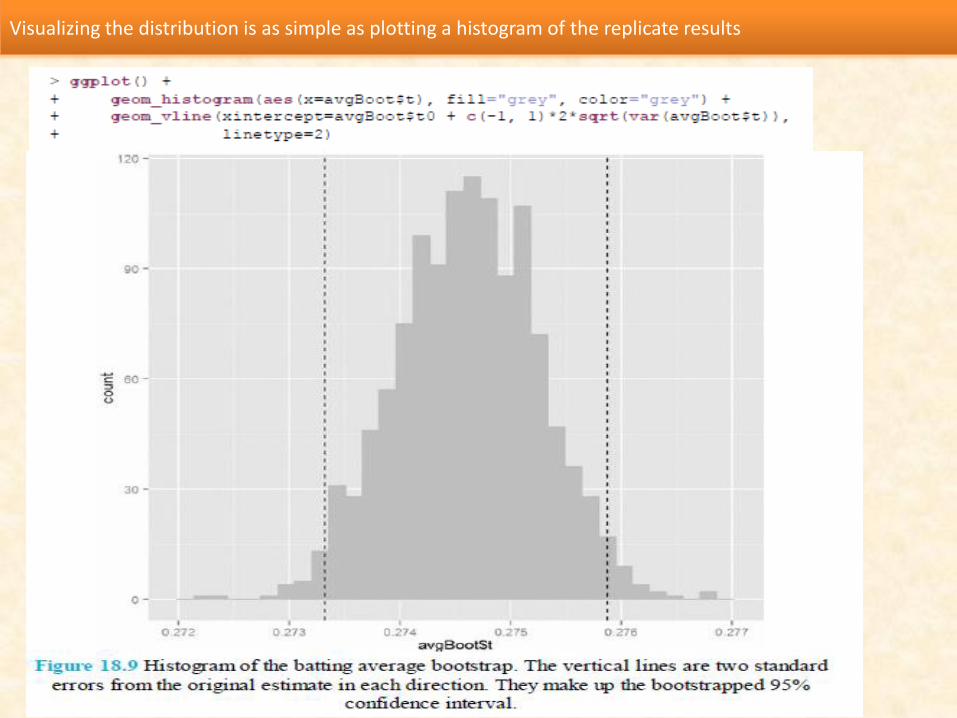
Visualizing the distribution is as simple as plotting a histogram of the replicate results

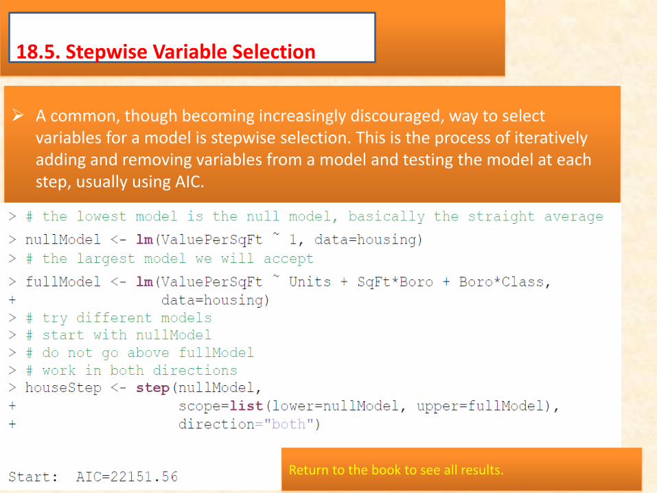
18.5. Stepwise Variable Selection

A common, though becoming increasingly discouraged, way to select variables for a model is stepwise selection. This is the process of iteratively adding and removing variables from a model and testing the model at each step, usually using AIC.

Return to the book to see all results.

Determining the quality of a model is an important step in the model-building process. This can take the form of traditional tests of fit such as ANOVA or more modern techniques like cross-validation.

The bootstrap is another means of determining model uncertainty, especially for models where confidence intervals are impractical to calculate. These can all be shaped by helping select which variables are included in a model and which are excluded.

18.6. Conclusion

Chapter 19. Regularization and Shrinkage

19.1. Elastic Net

a dynamic blending of lasso and ridge regression. The lasso uses an L1 penalty to perform variable selection and dimension

reduction, while the ridge uses an L2 penalty to shrink the coefficients for more stable predictions.

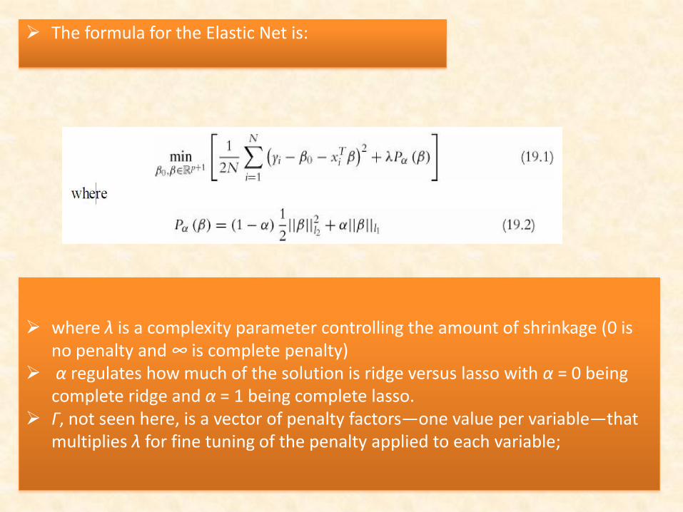
The formula for the Elastic Net is:

where λ is a complexity parameter controlling the amount of shrinkage (0 is no penalty and ∞ is complete penalty)

α regulates how much of the solution is ridge versus lasso with α = 0 being complete ridge and α = 1 being complete lasso.

Γ, not seen here, is a vector of penalty factors—one value per variable—that multiplies λ for fine tuning of the penalty applied to each variable;

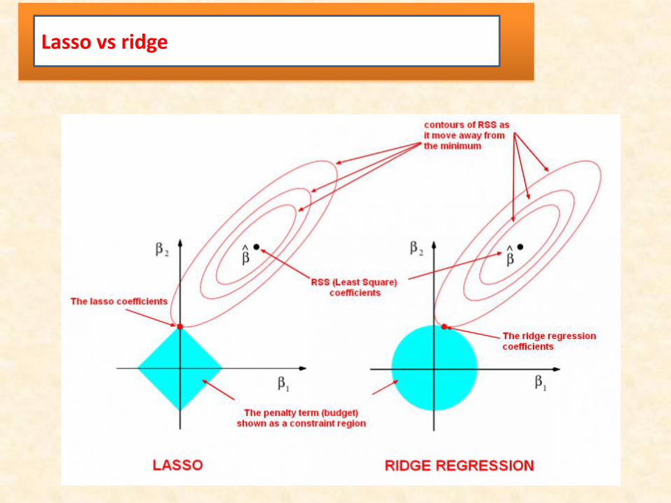
Lasso vs ridge

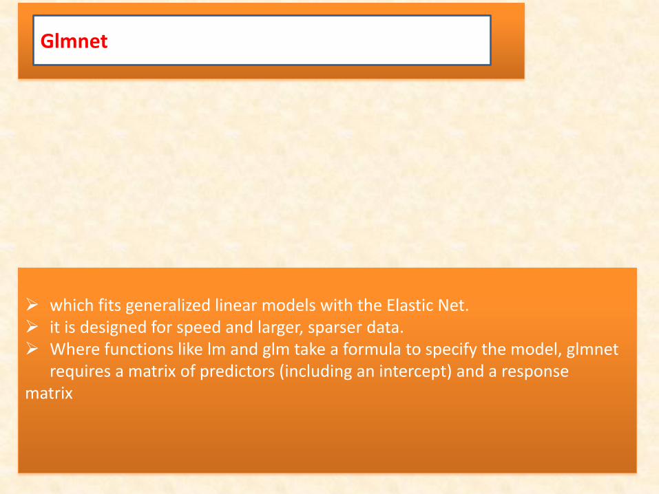
Glmnet

which fits generalized linear models with the Elastic Net. it is designed for speed and larger, sparser data. Where functions like lm and glm take a formula to specify the model, glmnet

requires a matrix of predictors (including an intercept) and a response matrix

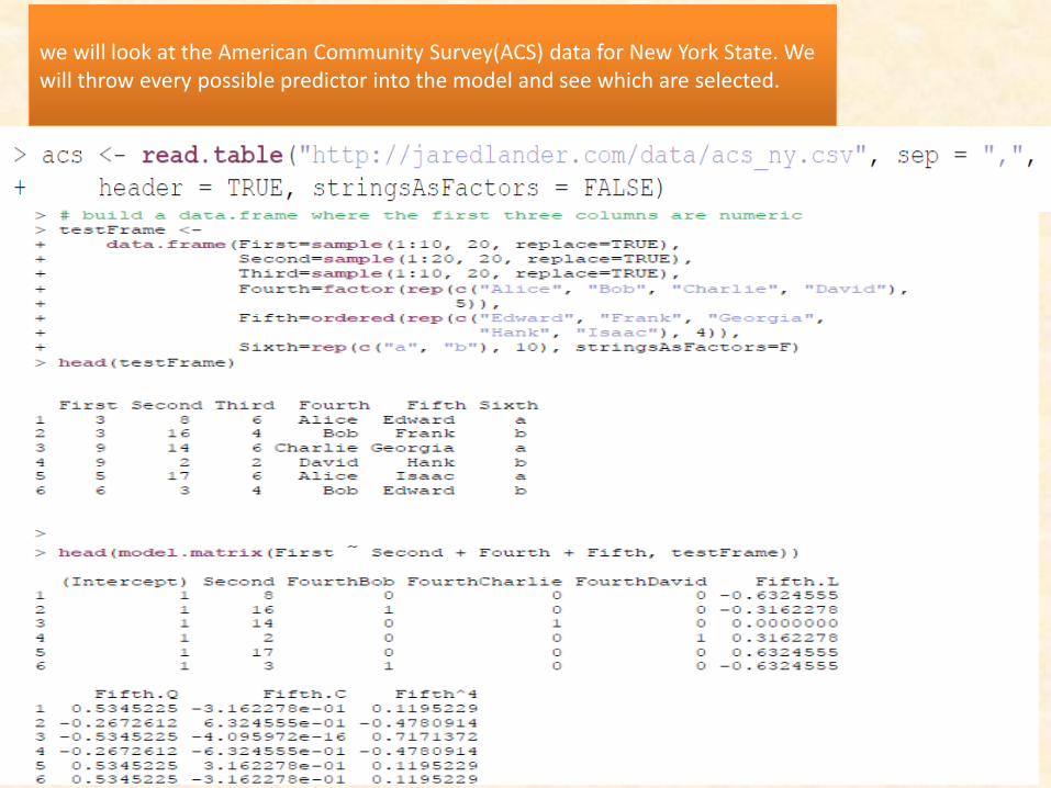
we will look at the American Community Survey(ACS) data for New York State. We will throw every possible predictor into the model and see which are selected.

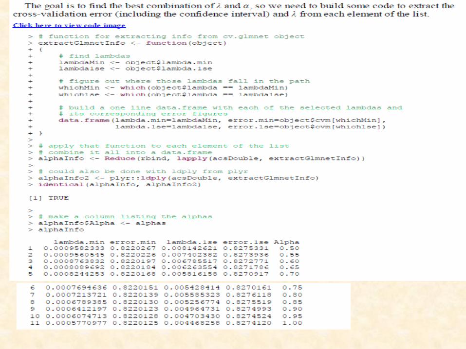
λ controls the amount of shrinkage. By default glmnet fits the regularization path on 100 different values of λ. glmnet package has a function, cv.glmnet, that computes the cross-validation automatically. By default α = 1, meaning only the lasso is calculated. Selecting the best α requires an additional layer of cross-validation.

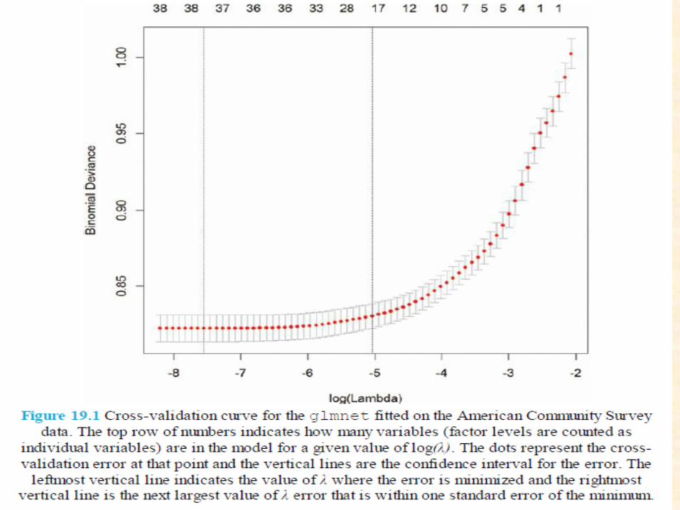
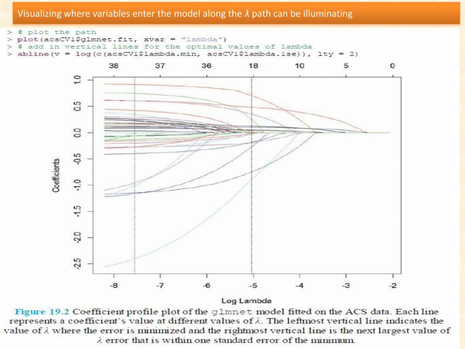
Visualizing where variables enter the model along the λ path can be illuminating

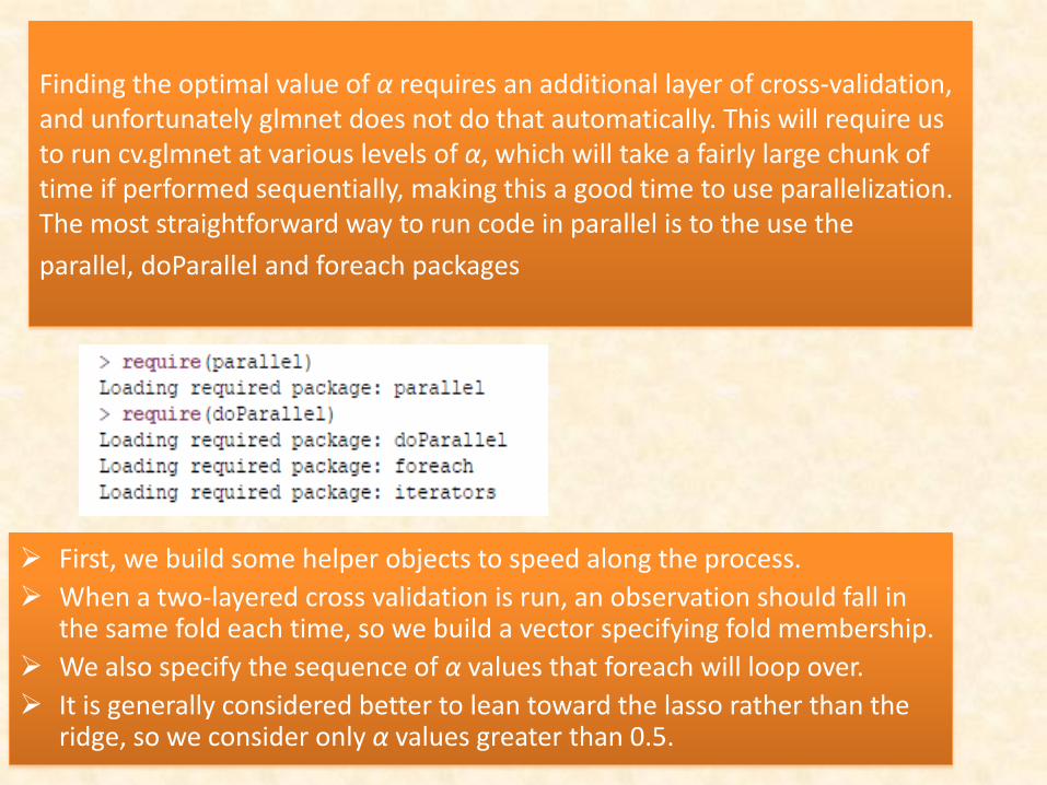
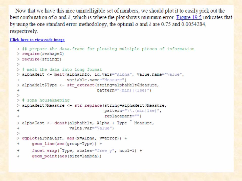
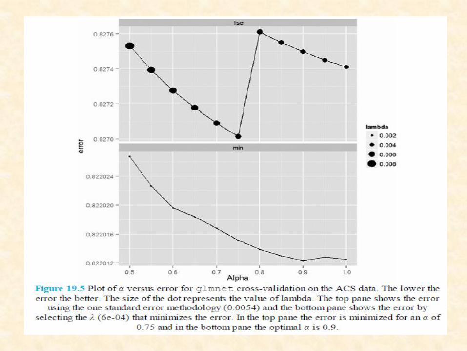
Finding the optimal value of α requires an additional layer of cross-validation, and unfortunately glmnet does not do that automatically. This will require us to run cv.glmnet at various levels of α, which will take a fairly large chunk of time if performed sequentially, making this a good time to use parallelization. The most straightforward way to run code in parallel is to the use the

parallel, doParallel and foreach packages

First, we build some helper objects to speed along the process.

When a two-layered cross validation is run, an observation should fall in the same fold each time, so we build a vector specifying fold membership.

We also specify the sequence of α values that foreach will loop over.

It is generally considered better to lean toward the lasso rather than the ridge, so we consider only α values greater than 0.5.

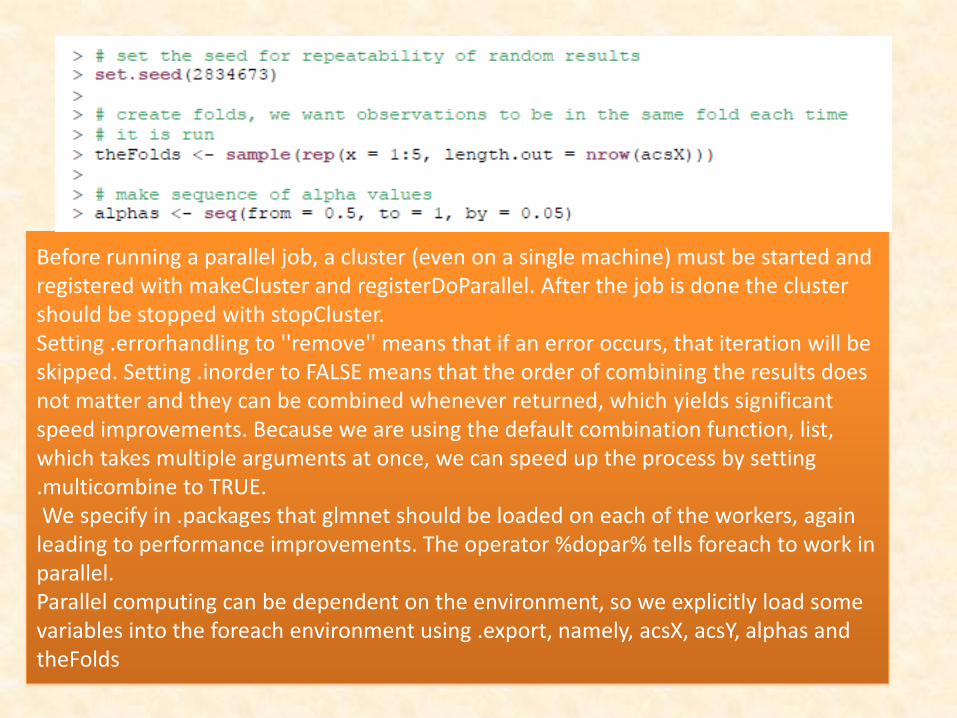
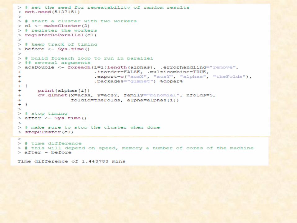
Before running a parallel job, a cluster (even on a single machine) must be started and registered with makeCluster and registerDoParallel. After the job is done the cluster should be stopped with stopCluster. Setting .errorhandling to ''remove'' means that if an error occurs, that iteration will be skipped. Setting .inorder to FALSE means that the order of combining the results does not matter and they can be combined whenever returned, which yields significant speed improvements. Because we are using the default combination function, list, which takes multiple arguments at once, we can speed up the process by setting .multicombine to TRUE. We specify in .packages that glmnet should be loaded on each of the workers, again leading to performance improvements. The operator %dopar% tells foreach to work in parallel. Parallel computing can be dependent on the environment, so we explicitly load some variables into the foreach environment using .export, namely, acsX, acsY, alphas and theFolds

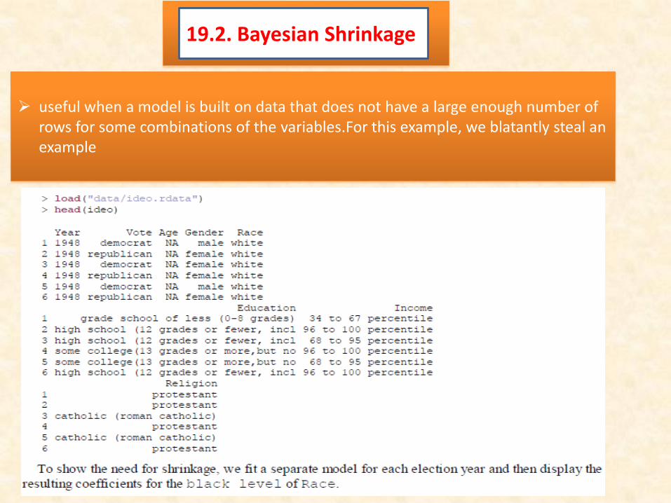
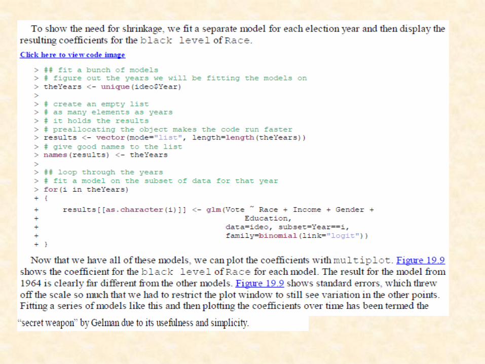
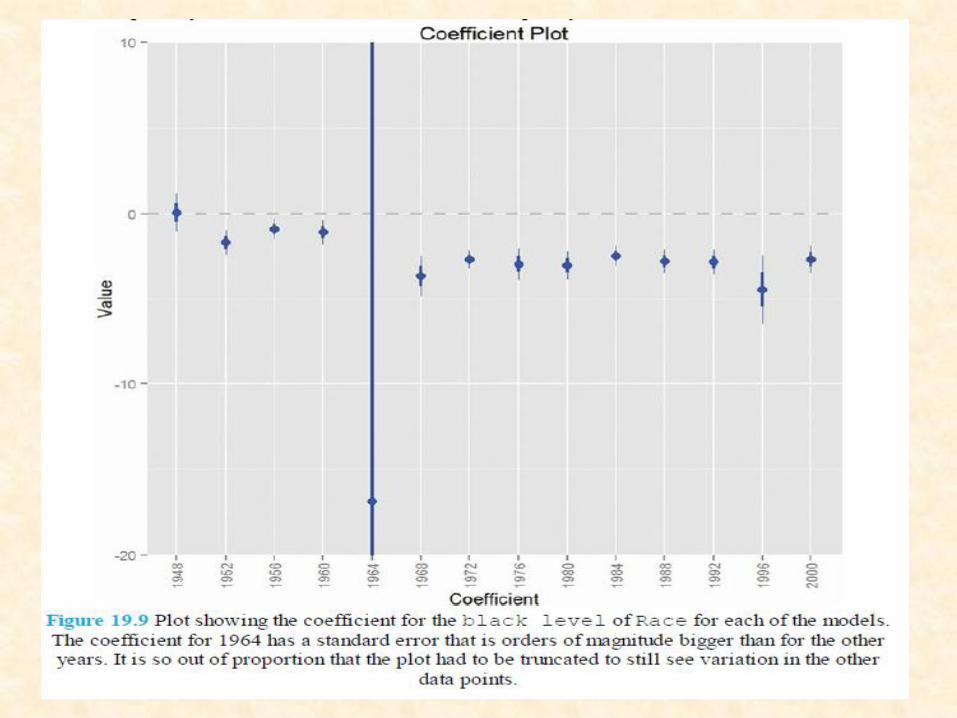
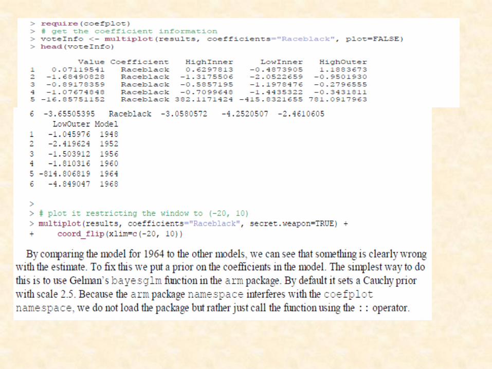
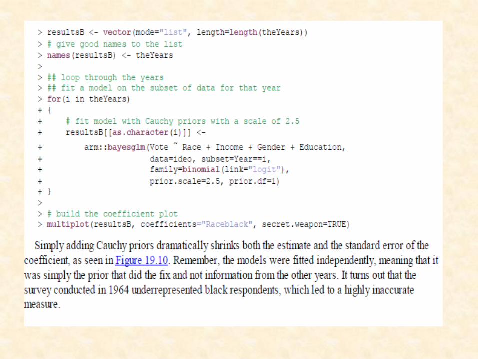
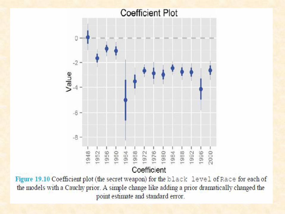
19.2. Bayesian Shrinkage

useful when a model is built on data that does not have a large enough number of rows for some combinations of the variables.For this example, we blatantly steal an example