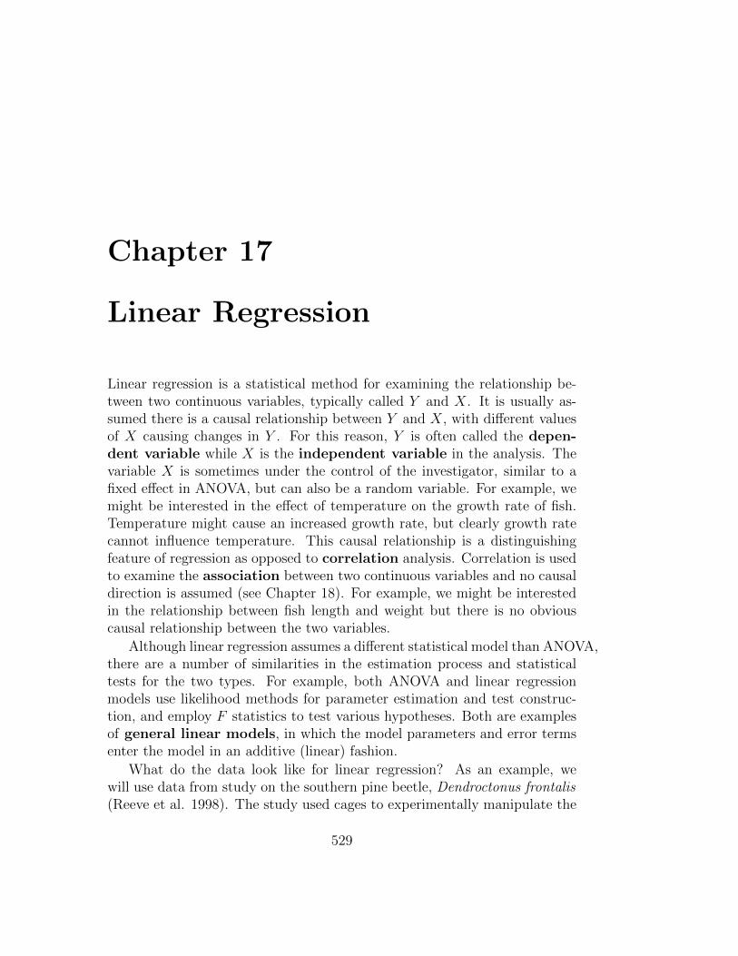
Chapter 17 Linear Regression Linear regression is a statistical method for examining the relationship be- tween two continuous variables, typically called Y and X . It is usually as- sumed there is a causal relationship between Y and X , with different values of X causing changes in Y . For this reason, Y is often called the depen- dent variable while X is the independent variable in the analysis. The variable X is sometimes under the control of the investigator, similar to a fixed effect in ANOVA, but can also be a random variable. For example, we might be interested in the effect of temperature on the growth rate of fish. Temperature might cause an increased growth rate, but clearly growth rate cannot influence temperature. This causal relationship is a distinguishing feature of regression as opposed to correlation analysis. Correlation is used to examine the association between two continuous variables and no causal direction is assumed (see Chapter 18). For example, we might be interested in the relationship between fish length and weight but there is no obvious causal relationship between the two variables. Although linear regression assumes a different statistical model than ANOVA, there are a number of similarities in the estimation process and statistical tests for the two types. For example, both ANOVA and linear regression models use likelihood methods for parameter estimation and test construc- tion, and employ F statistics to test various hypotheses. Both are examples of general linear models, in which the model parameters and error terms enter the model in an additive (linear) fashion. What do the data look like for linear regression? As an example, we will use data from study on the southern pine beetle, Dendroctonus frontalis (Reeve et al. 1998). The study used cages to experimentally manipulate the 529

Welcome message from author
This document is posted to help you gain knowledge. Please leave a comment to let me know what you think about it! Share it to your friends and learn new things together.
Transcript
Chapter 17
Linear Regression
Linear regression is a statistical method for examining the relationship be-tween two continuous variables, typically called Y and X. It is usually as-sumed there is a causal relationship between Y and X, with different valuesof X causing changes in Y . For this reason, Y is often called the depen-dent variable while X is the independent variable in the analysis. Thevariable X is sometimes under the control of the investigator, similar to afixed effect in ANOVA, but can also be a random variable. For example, wemight be interested in the effect of temperature on the growth rate of fish.Temperature might cause an increased growth rate, but clearly growth ratecannot influence temperature. This causal relationship is a distinguishingfeature of regression as opposed to correlation analysis. Correlation is usedto examine the association between two continuous variables and no causaldirection is assumed (see Chapter 18). For example, we might be interestedin the relationship between fish length and weight but there is no obviouscausal relationship between the two variables.
Although linear regression assumes a different statistical model than ANOVA,there are a number of similarities in the estimation process and statisticaltests for the two types. For example, both ANOVA and linear regressionmodels use likelihood methods for parameter estimation and test construc-tion, and employ F statistics to test various hypotheses. Both are examplesof general linear models, in which the model parameters and error termsenter the model in an additive (linear) fashion.
What do the data look like for linear regression? As an example, wewill use data from study on the southern pine beetle, Dendroctonus frontalis(Reeve et al. 1998). The study used cages to experimentally manipulate the
529
530 CHAPTER 17. LINEAR REGRESSION
density of D. frontalis attacking pine trees. The independent or X variable inthe study was the number of beetles added to the cages, while the dependentor Y variable was the number of attacks the beetles made through the barkinto the tree (Table 17.1). Besides establishing the relationship between thetwo variables, there was also some interest in predicting the attack densityas a function of the number of beetles added to the cage, for use in futurestudies. The notation Yi and Xi refers to the values for the ith pair ofnumbers. For example, Y2 = 2.660 and X2 = 1.000. Fig. 17.2 shows thereis a positive relationship between the two variables, with attack density (Y )increasing as more beetles are added to the cages (X).
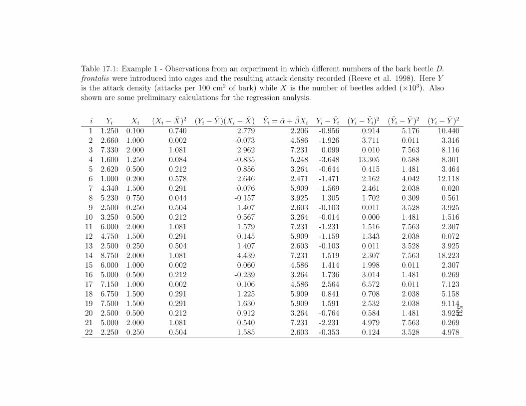
531Table 17.1: Example 1 - Observations from an experiment in which different numbers of the bark beetle D.frontalis were introduced into cages and the resulting attack density recorded (Reeve et al. 1998). Here Yis the attack density (attacks per 100 cm2 of bark) while X is the number of beetles added (×103). Alsoshown are some preliminary calculations for the regression analysis.
i Yi Xi (Xi − X)2 (Yi − Y )(Xi − X) Yi = α + βXi Yi − Yi (Yi − Yi)2 (Yi − Y )2 (Yi − Y )2
1 1.250 0.100 0.740 2.779 2.206 -0.956 0.914 5.176 10.4402 2.660 1.000 0.002 -0.073 4.586 -1.926 3.711 0.011 3.3163 7.330 2.000 1.081 2.962 7.231 0.099 0.010 7.563 8.1164 1.600 1.250 0.084 -0.835 5.248 -3.648 13.305 0.588 8.3015 2.620 0.500 0.212 0.856 3.264 -0.644 0.415 1.481 3.4646 1.000 0.200 0.578 2.646 2.471 -1.471 2.162 4.042 12.1187 4.340 1.500 0.291 -0.076 5.909 -1.569 2.461 2.038 0.0208 5.230 0.750 0.044 -0.157 3.925 1.305 1.702 0.309 0.5619 2.500 0.250 0.504 1.407 2.603 -0.103 0.011 3.528 3.925
10 3.250 0.500 0.212 0.567 3.264 -0.014 0.000 1.481 1.51611 6.000 2.000 1.081 1.579 7.231 -1.231 1.516 7.563 2.30712 4.750 1.500 0.291 0.145 5.909 -1.159 1.343 2.038 0.07213 2.500 0.250 0.504 1.407 2.603 -0.103 0.011 3.528 3.92514 8.750 2.000 1.081 4.439 7.231 1.519 2.307 7.563 18.22315 6.000 1.000 0.002 0.060 4.586 1.414 1.998 0.011 2.30716 5.000 0.500 0.212 -0.239 3.264 1.736 3.014 1.481 0.26917 7.150 1.000 0.002 0.106 4.586 2.564 6.572 0.011 7.12318 6.750 1.500 0.291 1.225 5.909 0.841 0.708 2.038 5.15819 7.500 1.500 0.291 1.630 5.909 1.591 2.532 2.038 9.11420 2.500 0.500 0.212 0.912 3.264 -0.764 0.584 1.481 3.92521 5.000 2.000 1.081 0.540 7.231 -2.231 4.979 7.563 0.26922 2.250 0.250 0.504 1.585 2.603 -0.353 0.124 3.528 4.978
532CHAPTER
17.LIN
EAR
REGRESSIO
N
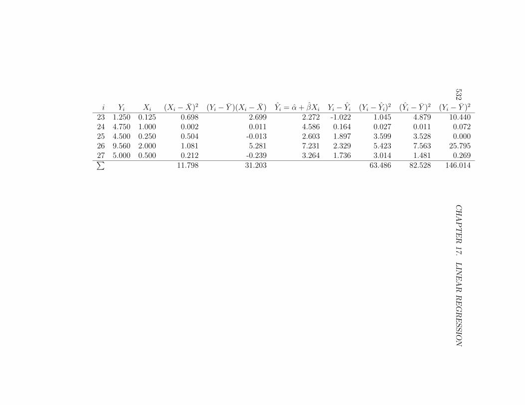
i Yi Xi (Xi − X)2 (Yi − Y )(Xi − X) Yi = α + βXi Yi − Yi (Yi − Yi)2 (Yi − Y )2 (Yi − Y )2
23 1.250 0.125 0.698 2.699 2.272 -1.022 1.045 4.879 10.44024 4.750 1.000 0.002 0.011 4.586 0.164 0.027 0.011 0.07225 4.500 0.250 0.504 -0.013 2.603 1.897 3.599 3.528 0.00026 9.560 2.000 1.081 5.281 7.231 2.329 5.423 7.563 25.79527 5.000 0.500 0.212 -0.239 3.264 1.736 3.014 1.481 0.269∑
11.798 31.203 63.486 82.528 146.014
17.1. LINEAR REGRESSION MODEL 533
17.1 Linear regression model
Suppose that we want to model the observations in studies like Example 1,where Y is observed for a number of X values. Let Yi and Xi stand for theith pair of values. The linear regression model takes the form
Yi = α + βXi + εi, (17.1)
where α is the intercept and β the slope of a line, while εi ∼ N(0, σ2) (Searle1971). Thus, the linear regression model represents the relationship betweenYi and Xi as a line on which random deviations due to natural variability(εi) are imposed.
For the ith pair of values, we have E[Yi] = α+βXi and V ar[Yi] = σ2 usingthe rules for expected values and variances. Thus, Yi ∼ N(α + βXi, σ
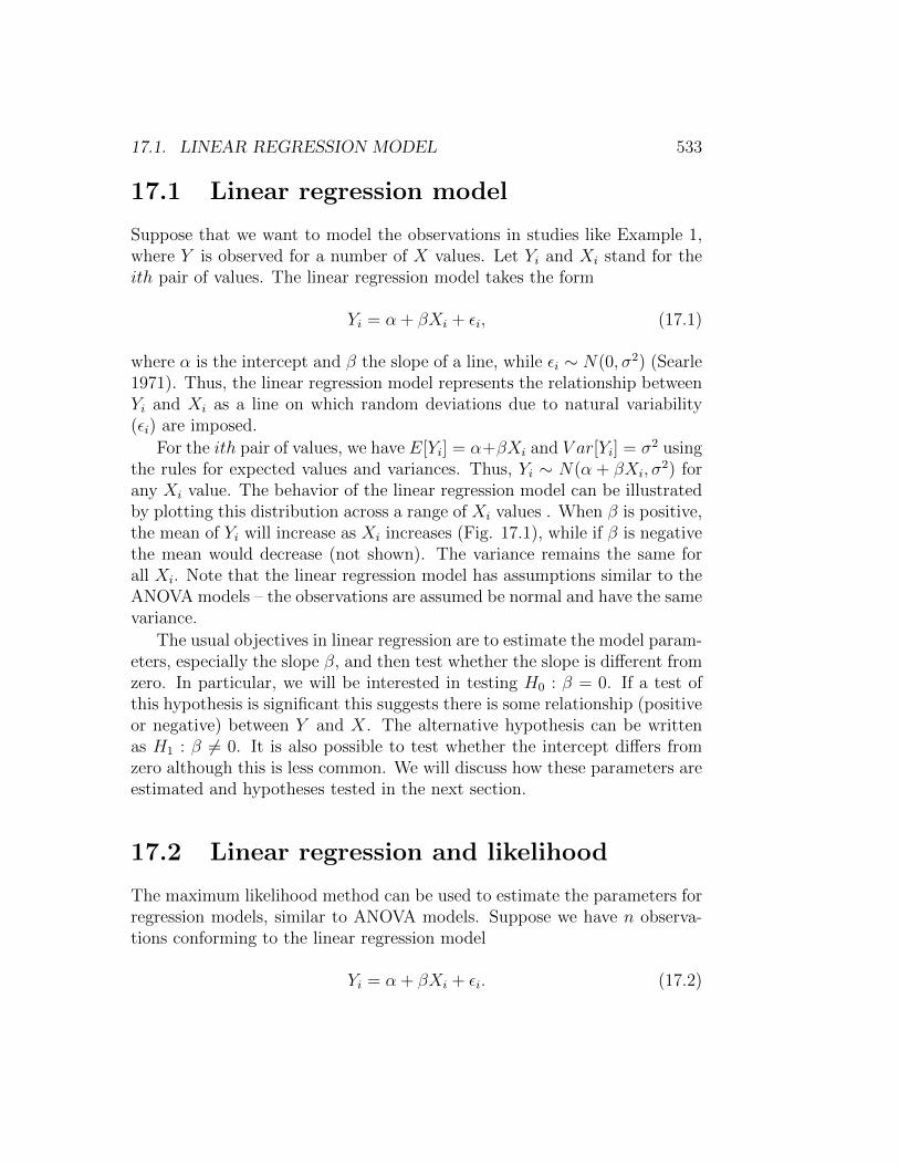
2) forany Xi value. The behavior of the linear regression model can be illustratedby plotting this distribution across a range of Xi values . When β is positive,the mean of Yi will increase as Xi increases (Fig. 17.1), while if β is negativethe mean would decrease (not shown). The variance remains the same forall Xi. Note that the linear regression model has assumptions similar to theANOVA models – the observations are assumed be normal and have the samevariance.
The usual objectives in linear regression are to estimate the model param-eters, especially the slope β, and then test whether the slope is different fromzero. In particular, we will be interested in testing H0 : β = 0. If a test ofthis hypothesis is significant this suggests there is some relationship (positiveor negative) between Y and X. The alternative hypothesis can be writtenas H1 : β 6= 0. It is also possible to test whether the intercept differs fromzero although this is less common. We will discuss how these parameters areestimated and hypotheses tested in the next section.
17.2 Linear regression and likelihood
The maximum likelihood method can be used to estimate the parameters forregression models, similar to ANOVA models. Suppose we have n observa-tions conforming to the linear regression model
Yi = α + βXi + εi. (17.2)
534 CHAPTER 17. LINEAR REGRESSION
Figure 17.1: The linear regression model plotted across a range of X values,with α = 2.0, β = 3.0, and σ2 = 2.5.
This model has three parameters to estimate, namely α, β, and σ2 (thevariance of εi). What would the likelihood function be for these data? Con-sider the first observation in the D. frontalis cage experiment, for whichY1 = 1.250 and X1 = 0.100. For this observation, the model states thatY1 ∼ N(α + βX1, σ
2), and so the likelihood would be
L1 =1√
2πσ2e−
12
(Y1−(α+βX1))2
σ2 =1√
2πσ2e−
12
(1.250−(α+β0.100))2
σ2 (17.3)
The likelihood Li for the ith observation would be similar, and the overalllikelihood is defined as their product:
L(α, β, σ2) = L1 × L2 × . . .× Ln. (17.4)
Finding the maximum likelihood estimates involves maximizing this quantitywith respect to the parameters α, β, and σ2. Using some calculus to find themaximum, it can be shown that estimators of these parameters are
β =
∑ni=1(Yi − Y )(Xi − X)∑n
i=1(Xi − X)2, (17.5)
α = Y − βX (17.6)
17.2. LINEAR REGRESSION AND LIKELIHOOD 535
and
σ2 =
∑ni=1(Yi − (α + βXi))
2
n− 2=
∑ni=1(Yi − Yi)2
n− 2. (17.7)
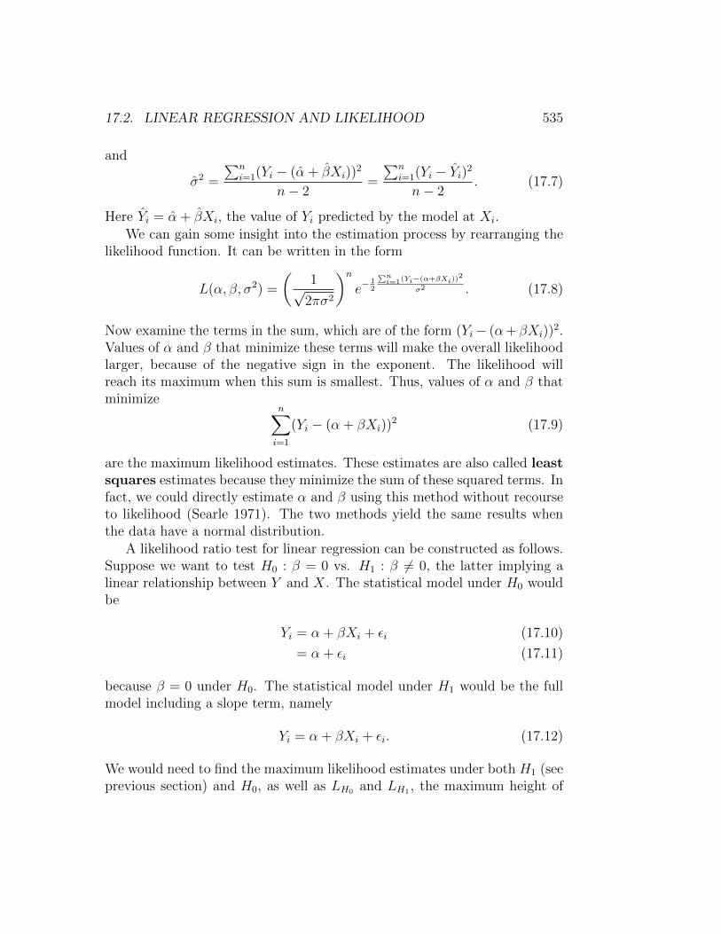
Here Yi = α + βXi, the value of Yi predicted by the model at Xi.We can gain some insight into the estimation process by rearranging the
likelihood function. It can be written in the form
L(α, β, σ2) =
(1√
2πσ2
)ne−
12
∑ni=1(Yi−(α+βXi))
2
σ2 . (17.8)
Now examine the terms in the sum, which are of the form (Yi− (α+ βXi))2.
Values of α and β that minimize these terms will make the overall likelihoodlarger, because of the negative sign in the exponent. The likelihood willreach its maximum when this sum is smallest. Thus, values of α and β thatminimize
n∑i=1
(Yi − (α + βXi))2 (17.9)
are the maximum likelihood estimates. These estimates are also called leastsquares estimates because they minimize the sum of these squared terms. Infact, we could directly estimate α and β using this method without recourseto likelihood (Searle 1971). The two methods yield the same results whenthe data have a normal distribution.
A likelihood ratio test for linear regression can be constructed as follows.Suppose we want to test H0 : β = 0 vs. H1 : β 6= 0, the latter implying alinear relationship between Y and X. The statistical model under H0 wouldbe
Yi = α + βXi + εi (17.10)
= α + εi (17.11)
because β = 0 under H0. The statistical model under H1 would be the fullmodel including a slope term, namely
Yi = α + βXi + εi. (17.12)
We would need to find the maximum likelihood estimates under both H1 (seeprevious section) and H0, as well as LH0 and LH1 , the maximum height of
536 CHAPTER 17. LINEAR REGRESSION
the likelihood function under H0 and H1. We would then use the likelihoodratio test statistic
λ =LH0
LH1
. (17.13)
There is a one-to-one correspondence between −2 ln(λ) and the statistic Fsused to test this null hypothesis (McCulloch & Searle 2001).
We can gain further insight into this test by defining various sum ofsquares and mean squares used to calculate Fs. In particular, we will defineSSerror, SSregression, and SStotal and their associated mean squares, whichhave functions similar to those in ANOVA. We will also summarize the cal-culations in an ANOVA table.
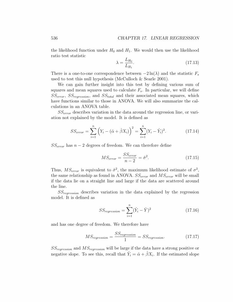
SSerror describes variation in the data around the regression line, or vari-ation not explained by the model. It is defined as
SSerror =n∑i=1
(Yi − (α + βXi)
)2
=n∑i=1
(Yi − Yi)2. (17.14)
SSerror has n− 2 degrees of freedom. We can therefore define
MSerror =SSerrorn− 2
= σ2. (17.15)
Thus, MSerror is equivalent to σ2, the maximum likelihood estimate of σ2,the same relationship as found in ANOVA. SSerror and MSerror will be smallif the data lie on a straight line and large if the data are scattered aroundthe line.
SSregression describes variation in the data explained by the regressionmodel. It is defined as
SSregression =n∑i=1
(Yi − Y )2 (17.16)
and has one degree of freedom. We therefore have
MSregression =SSregression
1= SSregression. (17.17)
SSregression and MSregression will be large if the data have a strong positive or
negative slope. To see this, recall that Yi = α + βXi. If the estimated slope
17.2. LINEAR REGRESSION AND LIKELIHOOD 537
β is large, the values of Yi will vary strongly as Xi changes and so generatea large sum of squares.
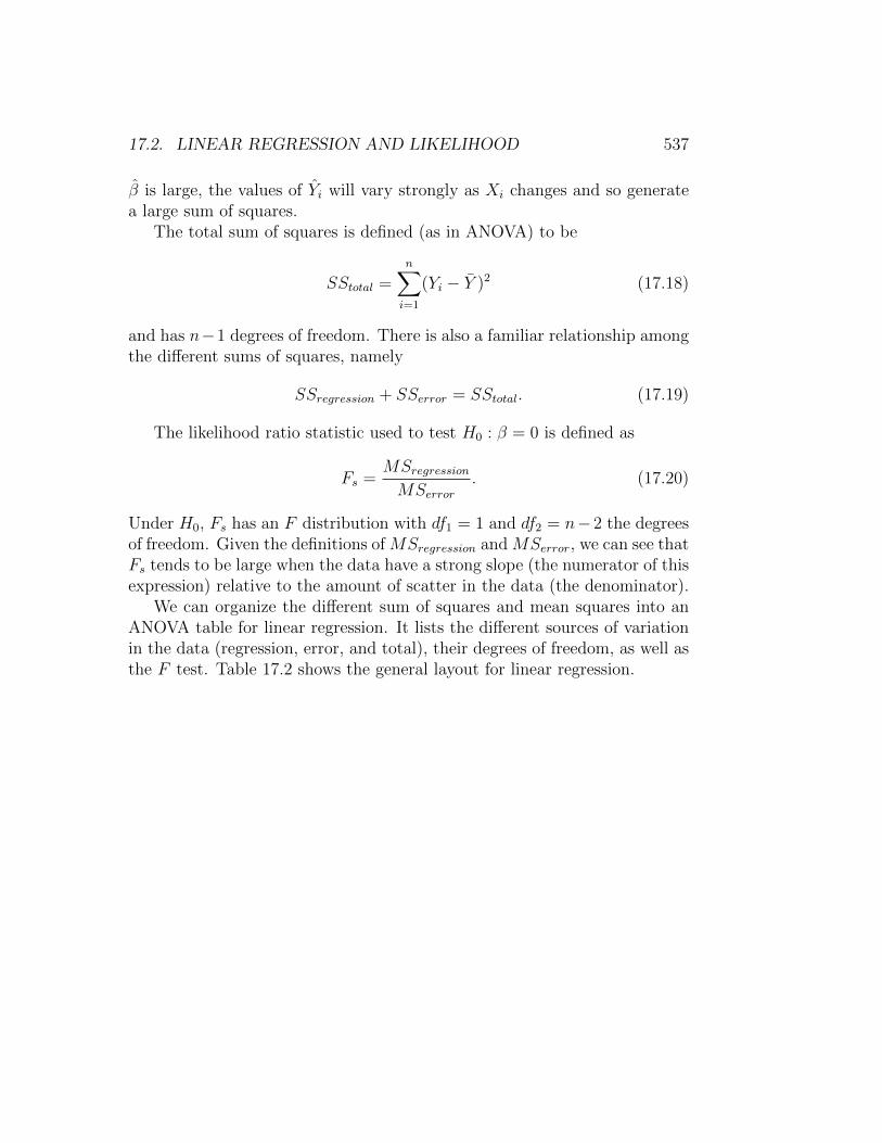
The total sum of squares is defined (as in ANOVA) to be
SStotal =n∑i=1
(Yi − Y )2 (17.18)
and has n−1 degrees of freedom. There is also a familiar relationship amongthe different sums of squares, namely
SSregression + SSerror = SStotal. (17.19)
The likelihood ratio statistic used to test H0 : β = 0 is defined as
Fs =MSregressionMSerror
. (17.20)
Under H0, Fs has an F distribution with df1 = 1 and df2 = n− 2 the degreesof freedom. Given the definitions of MSregression and MSerror, we can see thatFs tends to be large when the data have a strong slope (the numerator of thisexpression) relative to the amount of scatter in the data (the denominator).
We can organize the different sum of squares and mean squares into anANOVA table for linear regression. It lists the different sources of variationin the data (regression, error, and total), their degrees of freedom, as well asthe F test. Table 17.2 shows the general layout for linear regression.
538CHAPTER
17.LIN
EAR
REGRESSIO
N
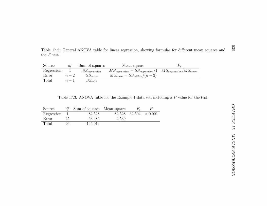
Table 17.2: General ANOVA table for linear regression, showing formulas for different mean squares andthe F test.
Source df Sum of squares Mean square FsRegression 1 SSregression MSregression = SSregression/1 MSregression/MSerrorError n− 2 SSerror MSerror = SSwithin/(n− 2)Total n− 1 SStotal
Table 17.3: ANOVA table for the Example 1 data set, including a P value for the test.
Source df Sum of squares Mean square Fs PRegression 1 82.528 82.528 32.504 < 0.001Error 25 63.486 2.539Total 26 146.014
17.2. LINEAR REGRESSION AND LIKELIHOOD 539
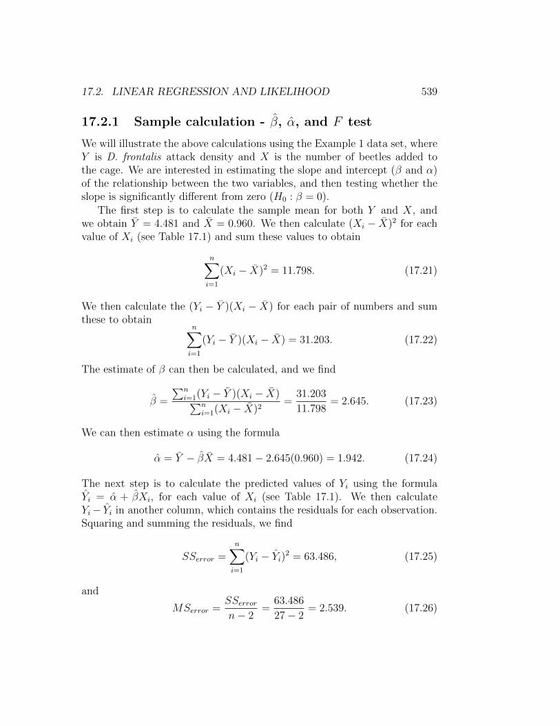
17.2.1 Sample calculation - β, α, and F test
We will illustrate the above calculations using the Example 1 data set, whereY is D. frontalis attack density and X is the number of beetles added tothe cage. We are interested in estimating the slope and intercept (β and α)of the relationship between the two variables, and then testing whether theslope is significantly different from zero (H0 : β = 0).
The first step is to calculate the sample mean for both Y and X, andwe obtain Y = 4.481 and X = 0.960. We then calculate (Xi − X)2 for eachvalue of Xi (see Table 17.1) and sum these values to obtain
n∑i=1
(Xi − X)2 = 11.798. (17.21)
We then calculate the (Yi − Y )(Xi − X) for each pair of numbers and sumthese to obtain
n∑i=1
(Yi − Y )(Xi − X) = 31.203. (17.22)
The estimate of β can then be calculated, and we find
β =
∑ni=1(Yi − Y )(Xi − X)∑n
i=1(Xi − X)2=
31.203
11.798= 2.645. (17.23)
We can then estimate α using the formula
α = Y − βX = 4.481− 2.645(0.960) = 1.942. (17.24)
The next step is to calculate the predicted values of Yi using the formulaYi = α + βXi, for each value of Xi (see Table 17.1). We then calculateYi− Yi in another column, which contains the residuals for each observation.Squaring and summing the residuals, we find
SSerror =n∑i=1
(Yi − Yi)2 = 63.486, (17.25)
and
MSerror =SSerrorn− 2
=63.486
27− 2= 2.539. (17.26)
540 CHAPTER 17. LINEAR REGRESSION
We next calculate a column consisting of (Yi− Y )2 for each observation, thensum these values to obtain
SSregression =n∑i=1
(Yi − Y )2 = 82.528, (17.27)
and soMSregression = SSregression/1 = 82.528. (17.28)
We are now in a position to calculate Fs, the statistic used to test H0 :β = 0. We have
Fs =MSregressionMSerror
=82.528
2.539= 32.504. (17.29)
Under H0, Fs has an F distribution with df1 = 1 and df2 = 27 − 2 = 25degrees of freedom. Using Table F, we find the P < 0.001. There is a highlysignificant effect of beetles numbers on the attack density of D. frontalis(F1,25 = 32.504, P < 0.001).
The last column in Table 17.1 calculates (Yi − Y )2, the components ofSStotal. Summing these components we obtain SStotal = 146.014. It can alsobe calculated using the formula SSregression + SSerror = SStotal. Table 17.3shows the completed ANOVA table.
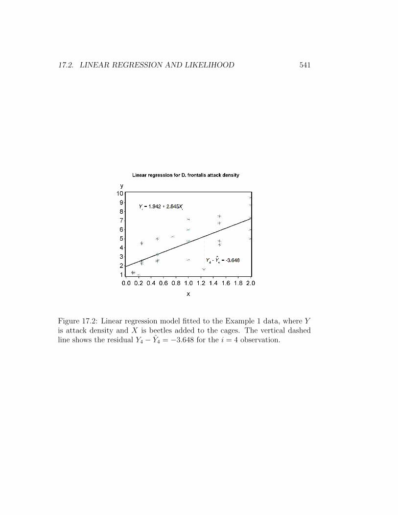
The observations for Example 1 and the fitted linear regression modelare shown in Fig. 17.2. The estimation procedure (maximum likelihood orleast squares) finds values of α and β that minimize the sum of the squareddifferences between the data points and the line. In particular, it minimizesthe sum of the squared residuals, where the residuals are Yi− Yi = Yi− (α+βXi).
17.2. LINEAR REGRESSION AND LIKELIHOOD 541
Figure 17.2: Linear regression model fitted to the Example 1 data, where Yis attack density and X is beetles added to the cages. The vertical dashedline shows the residual Y4 − Y4 = −3.648 for the i = 4 observation.
542 CHAPTER 17. LINEAR REGRESSION
17.3 Confidence and prediction intervals
In this section, we will examine confidence intervals for the parameters of theregression model, and for the mean value of Yi at a given value of Xi. Likeother confidence intervals, they provide a measure of the accuracy or reliabil-ity of an estimate, with wider intervals indicating lower accuracy (Chapter9). Another type of interval for linear regression are prediction intervals.These are used to set limits for future Yi values given some value of Xi. SeeDraper & Smith (1981) for further details.
The confidence interval for the slope β is based on β, the maximumlikelihood estimate of β, and the standard error of this estimate sβ, given bythe formula
sβ =
√σ2∑n
i=1(Xi − X)2, (17.30)
where σ2 = MSerror. Note that sβ depends on the scatter of the data around
the line (σ2) as well as the amount of variability in Xi. A study using alarger range of Xi values will thus provide a more accurate estimateof β, because it reduces sβ. Increasing the sample size n would alsoincrease the accuracy, by increasing the sum of squares in the denominatorfor sβ.
It can be shown that the quantity
β − βsβ
(17.31)
has a t distribution with n− 2 degrees of freedom, the same as for MSerror.This fact can be used to derive a confidence interval for β. Using Table T, wefirst find a value of cα,n−2 for n−2 degrees of freedom such that the followingequation is true:
P
[−cα,n−2 <
β − βsβ
< cα,n−2
]= 1− α. (17.32)
Rearranging this equation we obtain
P[β − cα,n−2sβ < β < β + cα,n−2sβ
]= 1− α. (17.33)
It follows that the interval
(β − cα,n−2sβ, β + cα,n−2sβ) (17.34)
17.3. CONFIDENCE AND PREDICTION INTERVALS 543
is a 100(1 − α)% confidence interval for β. The center of the confidenceinterval would be β.
We may also want to test various null hypotheses concerning β. Forexample, we may want to test H0 : β = β0 vs. H1 : β 6= β0, where β0 takessome value of interest. Similar to the approach in Chapter 10, we would usethe test statistic
Ts =β − β0
sβ. (17.35)
Under H0, Ts has a t distribution with n − 2 degrees of freedom, and wewould reject H0 for sufficiently large values of this statistic. For β0 = 0, thistest is equivalent to the F test we developed earlier for H0 : β = 0, and infact T 2
s = Fs. The t test is more general, however, because we can also testH0 : β = β0 for any value of β0.
It is possible to derive similar t tests and confidence intervals for theintercept parameter α. The t test is most commonly used to test H0 : α = 0.If the test is significant this implies an intercept different from zero. We willlet SAS handle the calculations here.
We can also derive a confidence interval for the theoretical mean of Yiat a given Xi value. Recall that according to the linear regression model,E[Yi] = α+βXi. Thus, Yi has a mean of µ = α+βXi for any Xi value. Theconfidence interval is based on Yi = α+ βXi, the predicted value of Yi at Xi.It also depends on the standard error sY of Y , which is given by the formula
sY =
√σ2
[1
n+
(Xi − X)2∑ni=1(Xi − X)2
]. (17.36)
Note that the standard error sY depends on the value of (Xi − X)2, whichis the squared distance of Xi from X. The farther Xi is from X, the largerthe value of sY .
Using methods similar to the confidence interval for β, it can be shownthat a 100(1− α) confidence interval for µ = α + βXi has the form
(Yi − cα,n−2sY , Yi + cα,n−2sY ). (17.37)
The interval will be broader for values of Xi far from X because sY will belarger. In other words, the precision of the confidence interval decreases withthe distance from X.
544 CHAPTER 17. LINEAR REGRESSION
Another type of interval associated with regression are prediction in-tervals. Here, we are trying to find an interval that contains a definedpercentage of future Yi values for a given value of Xi, hence the name pre-diction interval. These are similar in form to the intervals for the theoreticalmean µ = α + βXi, but are always wider because you are trying to enclosea single future observation rather than a mean value.
The prediction interval is based on Yi = α + βXi, the predicted value ofYi at Xi, and the standard error sY (1) of Yi, which is given by the formula
sY (1) =
√σ2
[1 +
1
n+
(Xi − X)2∑ni=1(Xi − X)2
]. (17.38)
Note the additional term (1+) within the square brackets, which makes thisstandard error larger than sY ). It also depends on the value of (Xi − X)2,and so the farther Xi is from X, the larger the value of sY (1). It can be shownthat a 100(1− α) prediction interval for a single future Yi has the form
(Yi − cα,n−2sY (1), Yi + cα,n−2sY (1)). (17.39)
17.3.1 Sample calculation - confidence and predictionintervals
We now illustrate the calculations for confidence intervals using the Example1 data. We earlier found that β = 2.645 and α = 1.942. To find a confidenceinterval for β, we first need to calculate sβ. From Table 17.1, we see that∑n
i=1(Xi − X)2 = 11.798, and we earlier calculated that σ2 = MSerror =2.539. Inserting these quantities into the formula for sβ, we find
sβ =
√σ2∑n
i=1(Xi − X)2=
√2.539
11.798= 0.464. (17.40)
For a 95% confidence interval and α = 0.05, the confidence interval for β hasthe form
(β − c0.05,n−2sβ, β + c0.05,n−2sβ) (17.41)
From Table T, with α = 0.05 and df = n − 2 = 27 − 2 = 25, we find thatc0.05,25 = 2.060. Inserting this value, β = 2.645, and sβ = 0.464 in thisformula, we obtain
(2.645− 2.060(0.464), 2.645 + 2.060(0.464)) (17.42)
17.3. CONFIDENCE AND PREDICTION INTERVALS 545
or(1.689, 3.601). (17.43)
We next find a confidence interval for the theoretical mean µ = α + βXi
at Xi = 0.5. For this value of Xi, we have
Yi = α + βXi = 1.942 + 2.645(0.5) = 3.265. (17.44)
From Table 17.1 we have∑n
i=1(Xi − X)2 = 11.798, and earlier found thatX = 0.960 and σ2 = MSerror = 2.539. Inserting these quantities into theformula for sY , we find that
sY =
√σ2
[1
n+
(Xi − X)2∑ni=1(Xi − X)2
](17.45)
=
√2.539
[1
27+
(0.5− 0.960)2
11.798
](17.46)
=
√2.539
[0.037 +
0.212
11.798
](17.47)
= 0.374. (17.48)
For a 95% confidence interval and α = 0.05, the confidence interval for thetheoretical mean µ = α + βXi has the form
(Y − c0.05,n−2sY , Y + c0.05,n−2sY ) (17.49)
From Table T with α = 0.05 and df = n − 2 = 27 − 2 = 25, we find thatc0.05,25 = 2.060. Inserting this value, Y = 3.265, and sY = 0.374 in thisformula, we find
(3.265− 2.060(0.374), 3.265 + 2.060(0.374)) (17.50)
or(2.495, 4.035). (17.51)
Lastly, we calculate a prediction interval for a single future observationYi at Xi = 0.5. For this value of Xi, we earlier calculated that
Yi = α + βXi = 1.942 + 2.645(0.5) = 3.265. (17.52)

546 CHAPTER 17. LINEAR REGRESSION
We again have∑n
i=1(Xi − X)2 = 11.798, X = 0.960 and σ2 = MSerror =2.539. Inserting these quantities into the formula for sY (1), we obtain
sY (1) =
√σ2
[1 +
1
n+
(Xi − X)2∑ni=1(Xi − X)2
](17.53)
=
√2.539
[1 +
1
27+
(0.5− 0.960)2
11.798
](17.54)
=
√2.539
[1 + 0.037 +
0.212
11.798
](17.55)
= 1.637. (17.56)
For a 95% prediction interval and α = 0.05, the interval has the form
(Y − c0.05,n−2sY (1), Y + c0.05,n−2sY (1)) (17.57)
From Table T with we have c0.05,25 = 2.060. Inserting c0.05,25 = 2.060, Y =3.265, and sY (1) = 1.637 in this formula, we obtain
(3.265− 2.060(1.637), 3.265 + 2.060(1.637)) (17.58)
or(−0.107, 6.637). (17.59)
Note this interval is much wider than the interval for the theoretical meanµ = α + βXi, which was (2.495, 4.035). This is because you are tryingto enclose a single future observation, a random variable Yi, rather than atheoretical mean.
17.4 R2 values
R2 values are a measure of how well a statistical model explains the data.Recall that the following relationship holds among the sum of squares inlinear regression:
SSregression + SSerror = SStotal. (17.60)
We can think of the different sum of squares as partitioning the variability inthe data into different sources. SSregression represents variability explained by
17.5. LINEAR REGRESSION FOR EXAMPLE 1 - SAS DEMO 547
the regression line, SSerror represents variability of the observations aroundthe regression line, while SStotal is the total amount of variability in thedata. The R2 value for a linear regression model is the proportion of totalvariability explained by the model, or
R2 =SSregressionSStotal
=SSregression
SSregression + SSerror. (17.61)
It is clear from this formula that R2 must range between 0 and 1 (0 ≤ R2 ≤1). For the Example 1 data, we have
R2 = 82.528/146.014 = 0.565. (17.62)
Thus, 56.5% of the variation is explained by the regression model for thesedata. Small R2 values indicate there is substantial variability in the data notexplained by the model, while large ones indicate the model explains mostof the variation.
More generally, we can define an R2 value for both ANOVA and regressionmodels as
R2 =SSmodelSStotal
=SSmodel
SSmodel + SSerror. (17.63)
For example, we have SSmodel = SSamong for one-way ANOVA while SSerror =SSwithin. The R2 value here is the proportion of the variation explained bythe one-way ANOVA model, in particular the variation among the groupmeans. The SAS output for proc glm provides an R2 for ANOVA models ofthis form.
17.5 Linear regression for Example 1 - SAS
demo
The linear regression analysis can be conducted using proc glm and a programsimilar in structure to ANOVA ones (see SAS program and output below).We first input the observations using a data step, applying transformations ifnecessary. The dependent variable Y is defined as the SAS variable y, whilethe independent variable X is defined as x. It is important to realizethat the actual names of these variables are not important - itis their position in proc gplot and proc glm that determines whichone is the dependent variable, and which is the independent one.
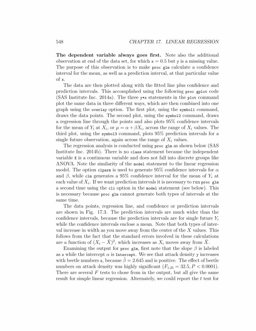
548 CHAPTER 17. LINEAR REGRESSION
The dependent variable always goes first. Note also the additionalobservation at end of the data set, for which x = 0.5 but y is a missing value.The purpose of this observation is to make proc glm calculate a confidenceinterval for the mean, as well as a prediction interval, at that particular valueof x.
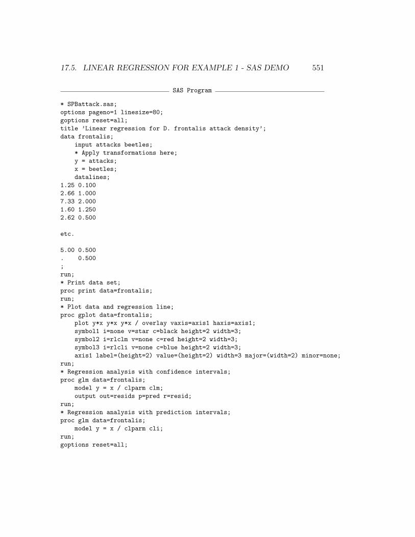
The data are then plotted along with the fitted line plus confidence andprediction intervals. This accomplished using the following proc gplot code(SAS Institute Inc. 2014a). The three y*x statements in the plot commandplot the same data in three different ways, which are then combined into onegraph using the overlay option. The first plot, using the symbol1 command,draws the data points. The second plot, using the symbol2 command, drawsa regression line through the points and also plots 95% confidence intervalsfor the mean of Yi at Xi, or µ = α+ βXi, across the range of Xi values. Thethird plot, using the symbol3 command, plots 95% prediction intervals for asingle future observation, again across the range of Xi values.
The regression analysis is conducted using proc glm as shown below (SASInstitute Inc. 2014b). There is no class statement because the independentvariable X is a continuous variable and does not fall into discrete groups likeANOVA. Note the similarity of the model statement to the linear regressionmodel. The option clparm is used to generate 95% confidence intervals for αand β, while clm generates a 95% confidence interval for the mean of Yi ateach value of Xi. If we want prediction intervals it is necessary to run proc glm
a second time using the cli option in the model statement (see below). Thisis necessary because proc glm cannot generate both types of intervals at thesame time.
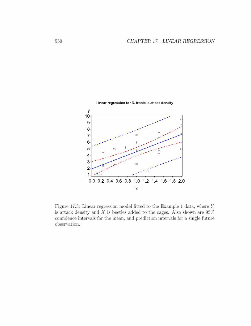
The data points, regression line, and confidence or prediction intervalsare shown in Fig. 17.3. The prediction intervals are much wider than theconfidence intervals, because the prediction intervals are for single future Yiwhile the confidence intervals enclose a mean. Note that both types of inter-val increase in width as you move away from the center of the X values. Thisfollows from the fact that the standard errors involved in these calculationsare a function of (Xi − X)2, which increases as Xi moves away from X.
Examining the output for proc glm, first note that the slope β is labeledas x while the intercept α is Intercept. We see that attack density y increaseswith beetle numbers x, because β = 2.645 and is positive. The effect of beetlenumbers on attack density was highly significant (F1,25 = 32.5, P < 0.0001).There are several F tests to chose from in the output, but all give the sameresult for simple linear regression. Alternately, we could report the t test for
17.5. LINEAR REGRESSION FOR EXAMPLE 1 - SAS DEMO 549
β (t25 = 5.70, P < 0.0001), which also tests H0 : β = 0. We see that R2 =0.565, indicating that 56.5% of the variation is explained by the regressionmodel.
The proc glm output also provides 95% confidence intervals for α and β.A 95% confidence interval for the mean of Yi at Xi = 0.5 is also given, andlabeled as 95% Confidence Limits for Mean Predicted Value. The second set ofoutput for proc glm contains a 95% prediction interval for a single future Yi atXi = 0.5, labeled as 95% Confidence Limits for Individual Predicted Value.
Note that the estimated intercept is some distance from zero (α = 1.942),and in fact the t test of H0 : α = 0 reported by SAS is highly significant(t25 = 3.59, P = 0.0014). This cannot really be true because the addition ofzero beetles should give you an attack density of zero. A more accurate (andpossibly non-linear) model would require that the intercept be zero.
This is a potential pitfall when using linear regression. Many biologicalphenomenon are approximately linear over some range of the data but theapproximation breaks down for more extreme values. A linear regressiondoes not take this possibility into account and so cannot provide a generalexplanation of some phenomena.
550 CHAPTER 17. LINEAR REGRESSION
Figure 17.3: Linear regression model fitted to the Example 1 data, where Yis attack density and X is beetles added to the cages. Also shown are 95%confidence intervals for the mean, and prediction intervals for a single futureobservation.
17.5. LINEAR REGRESSION FOR EXAMPLE 1 - SAS DEMO 551
SAS Program
* SPBattack.sas;
options pageno=1 linesize=80;
goptions reset=all;
title ’Linear regression for D. frontalis attack density’;
data frontalis;
input attacks beetles;
* Apply transformations here;
y = attacks;
x = beetles;
datalines;
1.25 0.100
2.66 1.000
7.33 2.000
1.60 1.250
2.62 0.500
etc.
5.00 0.500
. 0.500
;
run;
* Print data set;
proc print data=frontalis;
run;
* Plot data and regression line;
proc gplot data=frontalis;
plot y*x y*x y*x / overlay vaxis=axis1 haxis=axis1;
symbol1 i=none v=star c=black height=2 width=3;
symbol2 i=rlclm v=none c=red height=2 width=3;
symbol3 i=rlcli v=none c=blue height=2 width=3;
axis1 label=(height=2) value=(height=2) width=3 major=(width=2) minor=none;
run;
* Regression analysis with confidence intervals;
proc glm data=frontalis;
model y = x / clparm clm;
output out=resids p=pred r=resid;
run;
* Regression analysis with prediction intervals;
proc glm data=frontalis;
model y = x / clparm cli;
run;
goptions reset=all;

552 CHAPTER 17. LINEAR REGRESSION
title "Diagnostic plots to check ANOVA assumptions";
* Plot residuals vs. predicted values;
proc gplot data=resids;
plot resid*pred=1 / vaxis=axis1 haxis=axis1;
symbol1 v=star height=2 width=3;
axis1 label=(height=2) value=(height=2) width=3 major=(width=2) minor=none;
run;
* Normal quantile plot of residuals;
proc univariate noprint data=resids;
qqplot resid / normal waxis=3 height=4;
run;
quit;

17.5. LINEAR REGRESSION FOR EXAMPLE 1 - SAS DEMO 553
SAS Output
Linear regression for D. frontalis attack density 1
08:45 Sunday, November 14, 2010
Obs attacks beetles y x
1 1.25 0.100 1.25 0.100
2 2.66 1.000 2.66 1.000
3 7.33 2.000 7.33 2.000
4 1.60 1.250 1.60 1.250
5 2.62 0.500 2.62 0.500
etc.
27 5.00 0.500 5.00 0.500
28 . 0.500 . 0.500
Linear regression for D. frontalis attack density 2
08:45 Sunday, November 14, 2010
The GLM Procedure
Number of Observations Read 28
Number of Observations Used 27
Linear regression for D. frontalis attack density 3
08:45 Sunday, November 14, 2010
The GLM Procedure
Dependent Variable: y
Sum of
Source DF Squares Mean Square F Value Pr > F
Model 1 82.5283492 82.5283492 32.50 <.0001
Error 25 63.4855174 2.5394207
Corrected Total 26 146.0138667
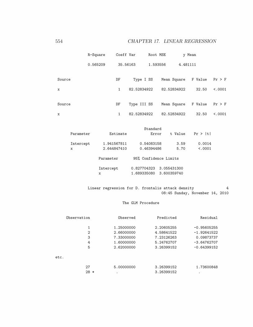
554 CHAPTER 17. LINEAR REGRESSION
R-Square Coeff Var Root MSE y Mean
0.565209 35.56163 1.593556 4.481111
Source DF Type I SS Mean Square F Value Pr > F
x 1 82.52834922 82.52834922 32.50 <.0001
Source DF Type III SS Mean Square F Value Pr > F
x 1 82.52834922 82.52834922 32.50 <.0001
Standard
Parameter Estimate Error t Value Pr > |t|
Intercept 1.941567811 0.54083158 3.59 0.0014
x 2.644847410 0.46394486 5.70 <.0001
Parameter 95% Confidence Limits
Intercept 0.827704323 3.055431300
x 1.689335080 3.600359740
Linear regression for D. frontalis attack density 4
08:45 Sunday, November 14, 2010
The GLM Procedure
Observation Observed Predicted Residual
1 1.25000000 2.20605255 -0.95605255
2 2.66000000 4.58641522 -1.92641522
3 7.33000000 7.23126263 0.09873737
4 1.60000000 5.24762707 -3.64762707
5 2.62000000 3.26399152 -0.64399152
etc.
27 5.00000000 3.26399152 1.73600848
28 * . 3.26399152 .
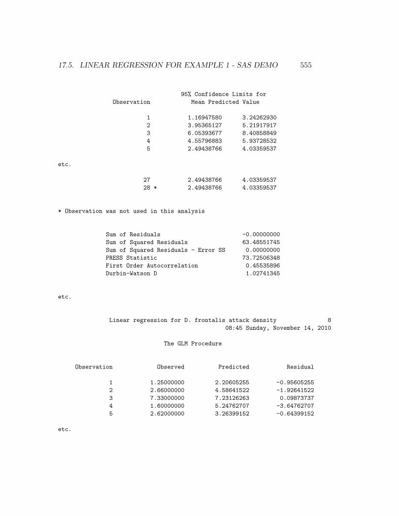
17.5. LINEAR REGRESSION FOR EXAMPLE 1 - SAS DEMO 555
95% Confidence Limits for
Observation Mean Predicted Value
1 1.16947580 3.24262930
2 3.95365127 5.21917917
3 6.05393677 8.40858849
4 4.55796883 5.93728532
5 2.49438766 4.03359537
etc.
27 2.49438766 4.03359537
28 * 2.49438766 4.03359537
* Observation was not used in this analysis
Sum of Residuals -0.00000000
Sum of Squared Residuals 63.48551745
Sum of Squared Residuals - Error SS 0.00000000
PRESS Statistic 73.72506348
First Order Autocorrelation 0.45535896
Durbin-Watson D 1.02741345
etc.
Linear regression for D. frontalis attack density 8
08:45 Sunday, November 14, 2010
The GLM Procedure
Observation Observed Predicted Residual
1 1.25000000 2.20605255 -0.95605255
2 2.66000000 4.58641522 -1.92641522
3 7.33000000 7.23126263 0.09873737
4 1.60000000 5.24762707 -3.64762707
5 2.62000000 3.26399152 -0.64399152
etc.
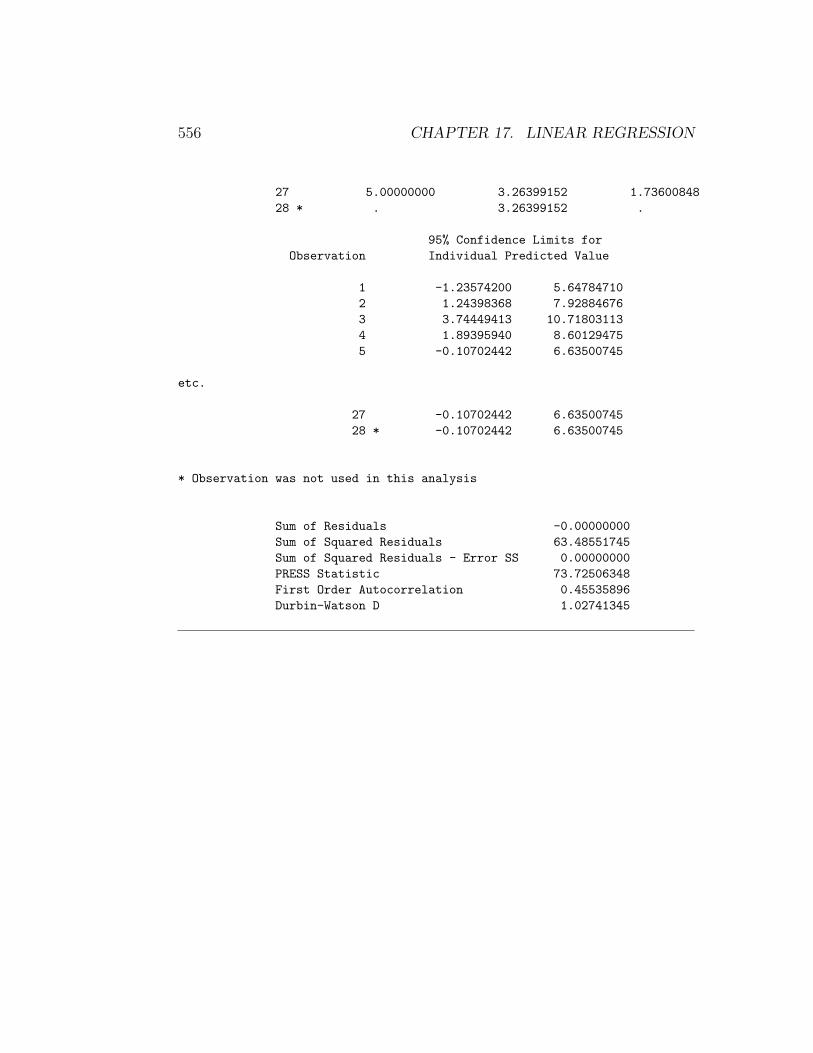
556 CHAPTER 17. LINEAR REGRESSION
27 5.00000000 3.26399152 1.73600848
28 * . 3.26399152 .
95% Confidence Limits for
Observation Individual Predicted Value
1 -1.23574200 5.64784710
2 1.24398368 7.92884676
3 3.74449413 10.71803113
4 1.89395940 8.60129475
5 -0.10702442 6.63500745
etc.
27 -0.10702442 6.63500745
28 * -0.10702442 6.63500745
* Observation was not used in this analysis
Sum of Residuals -0.00000000
Sum of Squared Residuals 63.48551745
Sum of Squared Residuals - Error SS 0.00000000
PRESS Statistic 73.72506348
First Order Autocorrelation 0.45535896
Durbin-Watson D 1.02741345
17.5. LINEAR REGRESSION FOR EXAMPLE 1 - SAS DEMO 557
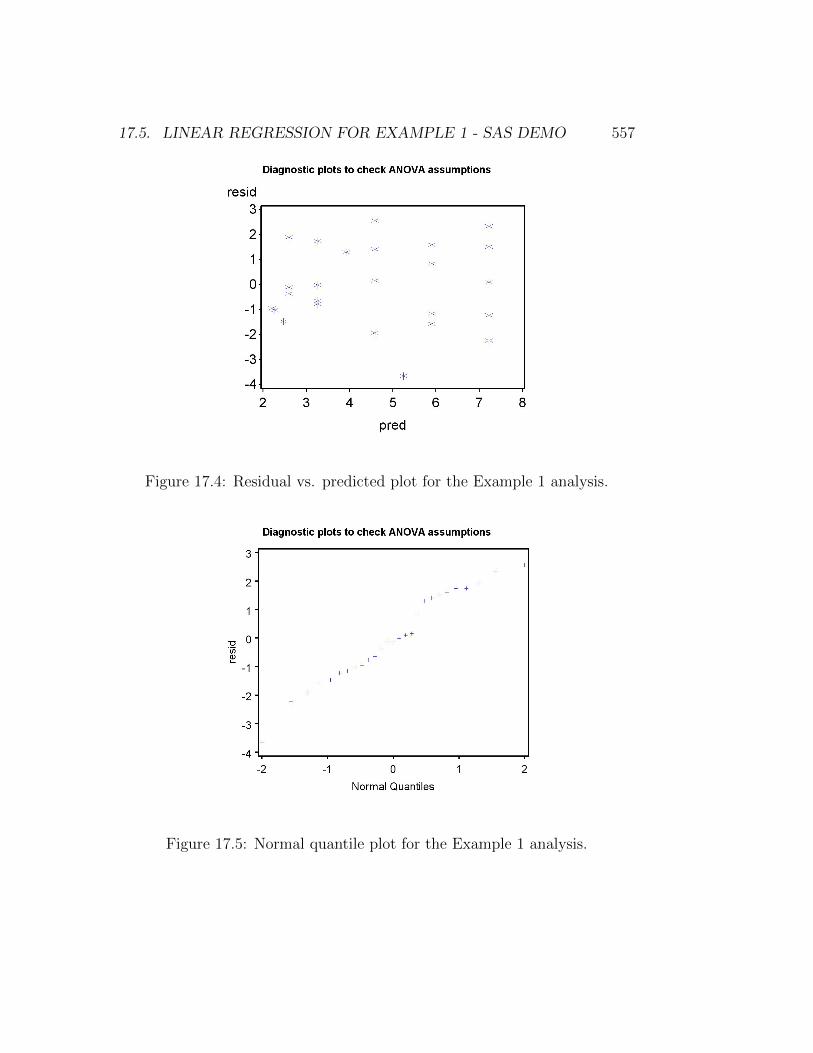
Figure 17.4: Residual vs. predicted plot for the Example 1 analysis.
Figure 17.5: Normal quantile plot for the Example 1 analysis.
558 CHAPTER 17. LINEAR REGRESSION
17.6 Assumptions and transformations
Linear regression makes the same assumptions as ANOVA, includ-ing homogeneity of variances and normality, and the same typesof plots can be used to assess them. If the homogeneity of variancesassumption is satisfied, the points in a residual vs. predicted plot shouldbe equally scattered across the range of predicted values. Outliers can alsobe identified using this plot. The normality assumption can be evaluatedusing a normal quantile plot of the residuals, with a straight diagonal lineindicating this assumption is satisfied.
Examining the residuals from the Example 1 analysis, we see no obviouspattern in the residual vs. predicted plot, suggesting the homogeneity ofvariances assumption is satisfied (Fig. 17.4). No outliers were present. Thenormal quantile plot suggests the normality assumption is satisfied (Fig.17.5).
Linear regression makes another key assumption, namely thatthe relationship between Y and X is linear. This assumption can bechecked by examining a plot of Y vs. X as well as the residual vs. predictedplot (see examples below). What can be done if the relationship seems non-linear? We can sometimes fix this problem by applying a transformation toY , X, or both Y and X, so that linear regression can be applied to the trans-formed data. This use of transformations greatly extends the utilityof linear regression. Some commonly used transformations are log Y vs.X, log Y vs. logX, Y vs. logX, and 1/Y vs. X. A transformation thatlinearizes the data sometimes corrects for problems with the homogeneity ofvariances and normality assumptions.
A transformation may be selected based on prior information about thedata and system. For example, a conservation biologist may be interestedin the relationship between island area A and the number of species S onthe island, and previous studies suggest the relationship between log10 S andlog10A will be linear (MacArthur & Wilson 1967). Another approach is totry a number of transformations and chose the one that makes the data mostlinear. We will illustrate each approach with an example below.
In cases where no transformation can linearize the data, another possi-bility would be nonlinear regression (Juliano 1993). This type of analysisrequires that the user specify a model Y = f(X, θ1, θ2, . . .) + ε for the data,where f is a function with parameters θ1, θ2, . . . to be estimated. SAS imple-ments this type of nonlinear regression in proc nlin, while proc nlmixed allows
17.6. ASSUMPTIONS AND TRANSFORMATIONS 559
for nonlinear functions as well as random effects and nonnormal distributions.
17.6.1 Species-area data - SAS demo
For many organisms there is a relationship between a defined area of habitat,such as an island, and the number of species found there. If S is the numberof species, and A the area of habitat, then the model S = cAz seems todescribe many data sets (MacArthur & Wilson 1967). Taking the log10 ofboth sides of this equation, we obtain
log10 S = log10 c+ z log10A. (17.64)
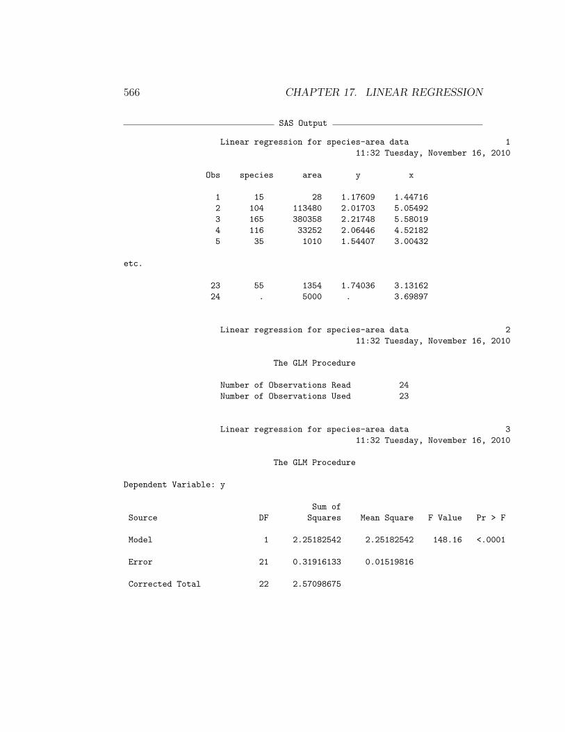
This form of the model is linear and suggests linear regression could be usedto analyze species-area data. The SAS program listed below shows howthese transformations can be applied to the bird fauna on archipelagos andislands of varying areas. The data are the number of species vs. island area(square miles) for 23 islands. The data were simulated to resemble Fig. 9in MacArthur & Wilson (1967). An extra observation is included with amissing value for the number of species, but an island area of 5000 squaremiles, to make proc glm calculate a confidence interval for the mean of thisisland.
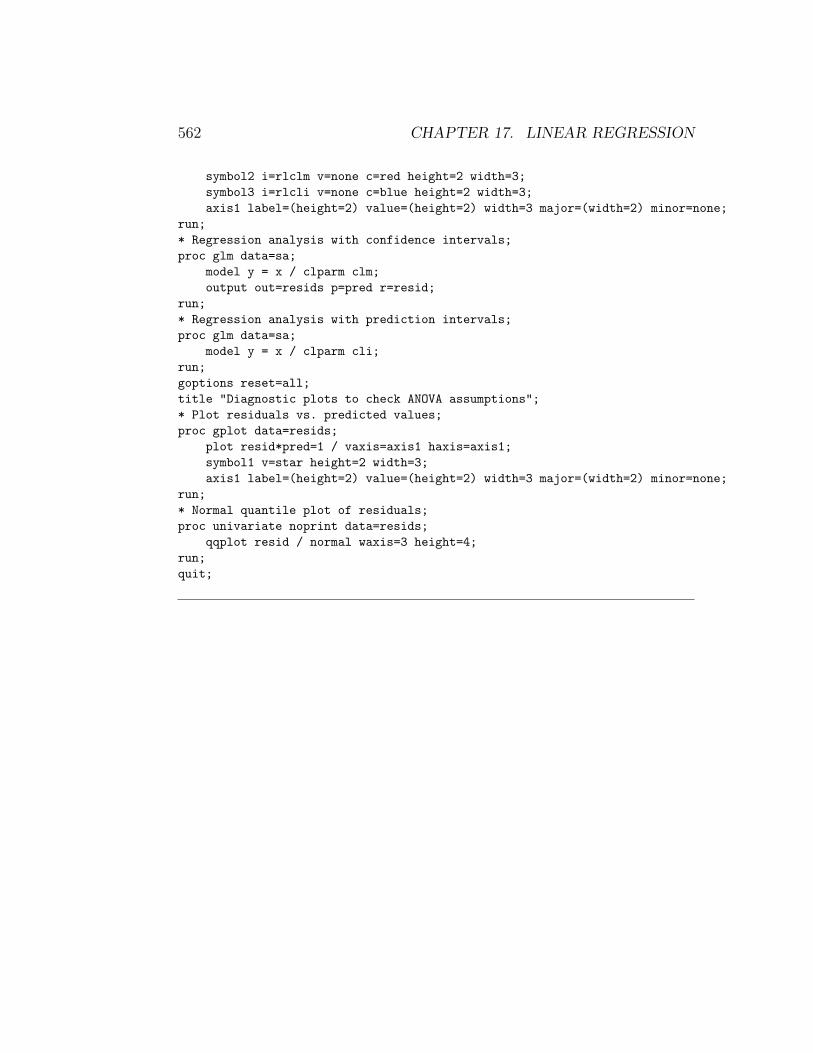
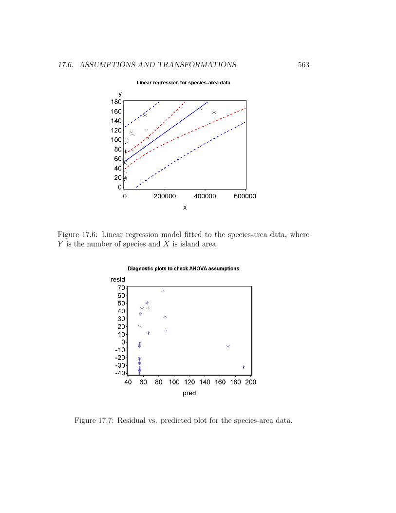
We first conduct the analysis without any transformation and examinethe gplot graph of Y vs. X, where Y is the number of species and X is islandarea (Fig. 17.6). Note the nonlinear nature of the relationship between thenumber of species and island area. This pattern is also reflected in theresidual vs. predicted plot (Fig. 17.7), which appears to be hump-shaped.Both plots suggest that a transformation is required for these data in orderto linearize the relationship between the two variables.
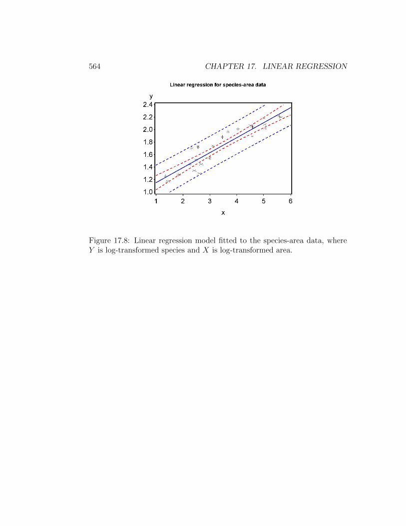
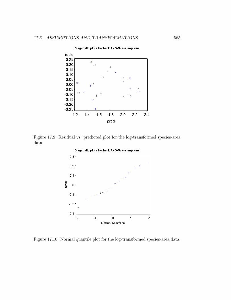
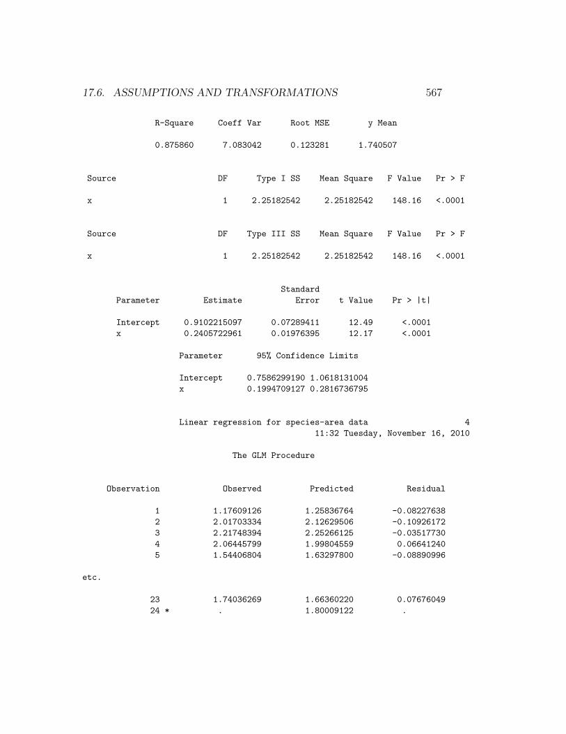
The picture improves after a log10 transformation is applied to bothspecies and area. We see that the graph of the transformed variables islinear (Fig. 17.8) and residual vs. predicted plot is featureless (Fig. 17.9).The normal quantile plot is also well-behaved (Fig. 17.10). Now that thevarious assumptions are satisfied we can interpret the rest of the SAS output(see below). We see that the number of species increases with island area(β = 0.241) and the effect is highly significant (F1,21 = 148.16, P < 0.0001).
In terms of the original model, where S = cAz, we see that β = 0.241 isalso an estimate of z. The R2 value is 0.876, indicating that 87.6% of thevariation is explained by the regression model. Confidence intervals are alsoprovided for the intercept and slope.
560 CHAPTER 17. LINEAR REGRESSION
The proc glm output also generates a predicted value Yi = 1.800 at Xi =3.699 (log10 5000 = 3.699). We need to convert this to the original scale
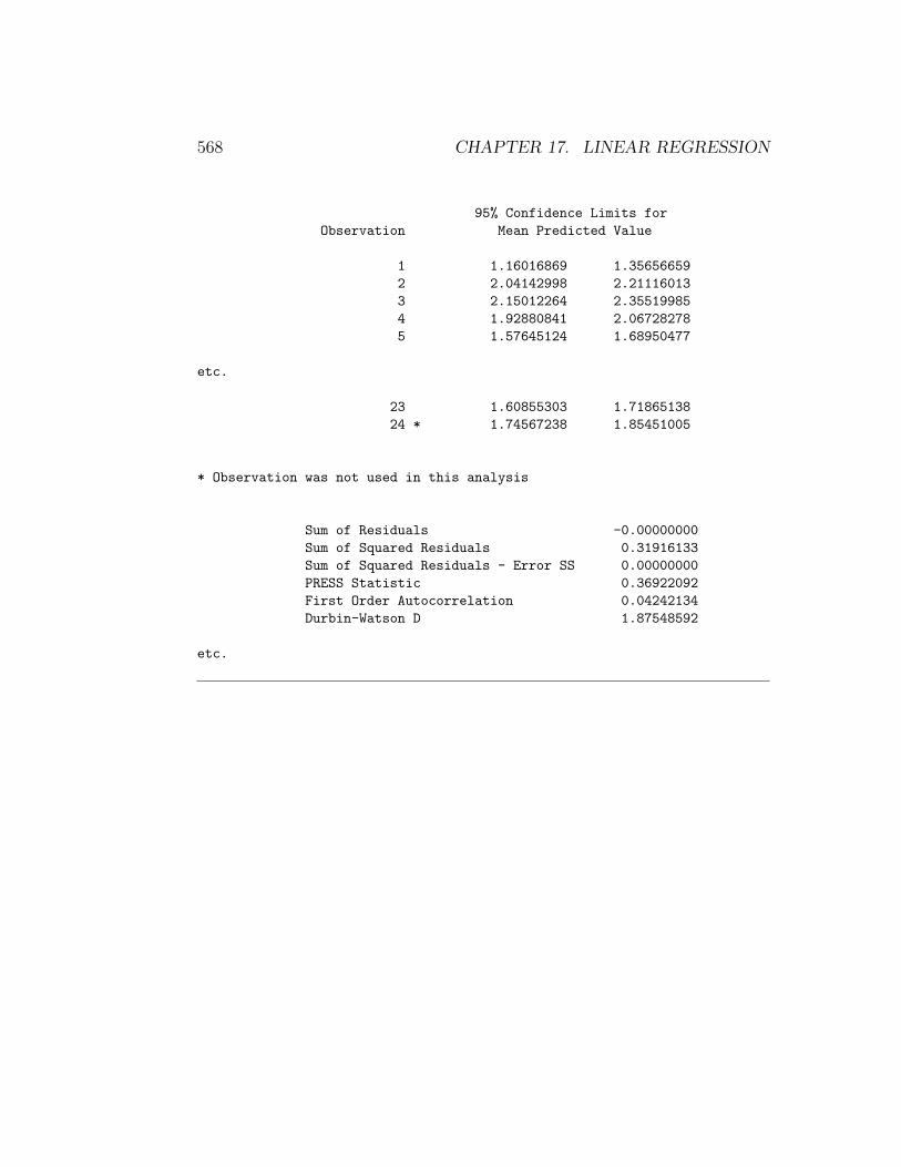
measurement using antilogs. We have Si = 10Yi = 101.800 = 63.10 species.So, we predict there would be 63 species on an island of 5000 square miles.The confidence interval for the mean is (1.746, 1.855), which we can similarlyconvert to (101.745, 101.855) or (55.72, 71.61).
17.6. ASSUMPTIONS AND TRANSFORMATIONS 561
SAS Program
* SAprob2.sas;
options pageno=1 linesize=80;
goptions reset=all;
title ’Linear regression for species-area data’;
data sa;
input species area;
* Apply transformations here;
y = log10(species);
x = log10(area);
datalines;
15 28
104 113480
165 380358
116 33252
35 1010
33 305
78 37620
93 4762
50 213
76 2976
18 23
28 186
20 423
121 108512
53 364
22 269
102 11163
28 487
158 445409
19 70
111 38309
152 100873
55 1354
. 5000
;
run;
* Print data set;
proc print data=sa;
run;
* Plot data and regression line;
proc gplot data=sa;
plot y*x=1 y*x=2 y*x=3 / overlay vaxis=axis1 haxis=axis1;
symbol1 i=none v=star c=black height=2 width=3;
562 CHAPTER 17. LINEAR REGRESSION
symbol2 i=rlclm v=none c=red height=2 width=3;
symbol3 i=rlcli v=none c=blue height=2 width=3;
axis1 label=(height=2) value=(height=2) width=3 major=(width=2) minor=none;
run;
* Regression analysis with confidence intervals;
proc glm data=sa;
model y = x / clparm clm;
output out=resids p=pred r=resid;
run;
* Regression analysis with prediction intervals;
proc glm data=sa;
model y = x / clparm cli;
run;
goptions reset=all;
title "Diagnostic plots to check ANOVA assumptions";
* Plot residuals vs. predicted values;
proc gplot data=resids;
plot resid*pred=1 / vaxis=axis1 haxis=axis1;
symbol1 v=star height=2 width=3;
axis1 label=(height=2) value=(height=2) width=3 major=(width=2) minor=none;
run;
* Normal quantile plot of residuals;
proc univariate noprint data=resids;
qqplot resid / normal waxis=3 height=4;
run;
quit;
17.6. ASSUMPTIONS AND TRANSFORMATIONS 563
Figure 17.6: Linear regression model fitted to the species-area data, whereY is the number of species and X is island area.
Figure 17.7: Residual vs. predicted plot for the species-area data.
564 CHAPTER 17. LINEAR REGRESSION
Figure 17.8: Linear regression model fitted to the species-area data, whereY is log-transformed species and X is log-transformed area.
17.6. ASSUMPTIONS AND TRANSFORMATIONS 565
Figure 17.9: Residual vs. predicted plot for the log-transformed species-areadata.
Figure 17.10: Normal quantile plot for the log-transformed species-area data.
566 CHAPTER 17. LINEAR REGRESSION
SAS Output
Linear regression for species-area data 1
11:32 Tuesday, November 16, 2010
Obs species area y x
1 15 28 1.17609 1.44716
2 104 113480 2.01703 5.05492
3 165 380358 2.21748 5.58019
4 116 33252 2.06446 4.52182
5 35 1010 1.54407 3.00432
etc.
23 55 1354 1.74036 3.13162
24 . 5000 . 3.69897
Linear regression for species-area data 2
11:32 Tuesday, November 16, 2010
The GLM Procedure
Number of Observations Read 24
Number of Observations Used 23
Linear regression for species-area data 3
11:32 Tuesday, November 16, 2010
The GLM Procedure
Dependent Variable: y
Sum of
Source DF Squares Mean Square F Value Pr > F
Model 1 2.25182542 2.25182542 148.16 <.0001
Error 21 0.31916133 0.01519816
Corrected Total 22 2.57098675
17.6. ASSUMPTIONS AND TRANSFORMATIONS 567
R-Square Coeff Var Root MSE y Mean
0.875860 7.083042 0.123281 1.740507
Source DF Type I SS Mean Square F Value Pr > F
x 1 2.25182542 2.25182542 148.16 <.0001
Source DF Type III SS Mean Square F Value Pr > F
x 1 2.25182542 2.25182542 148.16 <.0001
Standard
Parameter Estimate Error t Value Pr > |t|
Intercept 0.9102215097 0.07289411 12.49 <.0001
x 0.2405722961 0.01976395 12.17 <.0001
Parameter 95% Confidence Limits
Intercept 0.7586299190 1.0618131004
x 0.1994709127 0.2816736795
Linear regression for species-area data 4
11:32 Tuesday, November 16, 2010
The GLM Procedure
Observation Observed Predicted Residual
1 1.17609126 1.25836764 -0.08227638
2 2.01703334 2.12629506 -0.10926172
3 2.21748394 2.25266125 -0.03517730
4 2.06445799 1.99804559 0.06641240
5 1.54406804 1.63297800 -0.08890996
etc.
23 1.74036269 1.66360220 0.07676049
24 * . 1.80009122 .
568 CHAPTER 17. LINEAR REGRESSION
95% Confidence Limits for
Observation Mean Predicted Value
1 1.16016869 1.35656659
2 2.04142998 2.21116013
3 2.15012264 2.35519985
4 1.92880841 2.06728278
5 1.57645124 1.68950477
etc.
23 1.60855303 1.71865138
24 * 1.74567238 1.85451005
* Observation was not used in this analysis
Sum of Residuals -0.00000000
Sum of Squared Residuals 0.31916133
Sum of Squared Residuals - Error SS 0.00000000
PRESS Statistic 0.36922092
First Order Autocorrelation 0.04242134
Durbin-Watson D 1.87548592
etc.
17.6. ASSUMPTIONS AND TRANSFORMATIONS 569
17.6.2 Population growth rates - SAS demo
As another example of transformations, consider a study of the populationgrowth of phytophagous mites on leaf sections. An experiment is conductedin which leaf sections are inoculated with a range of mite densities and thenumber of offspring recorded one generation later. The number of offspringper initial mite is the finite growth of the population, usually symbolized asλ. The SAS program listed below gives the mite densities and the λ valuesfor this experiment.
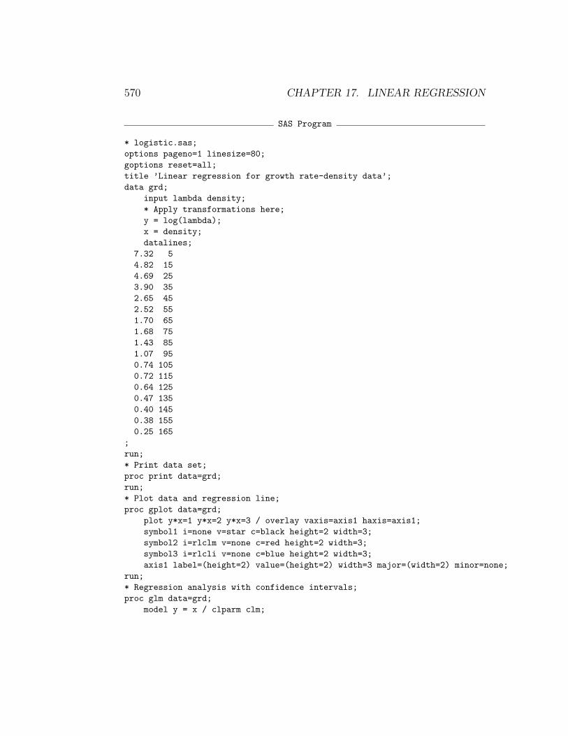
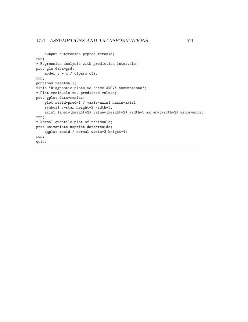
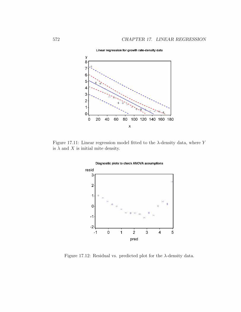
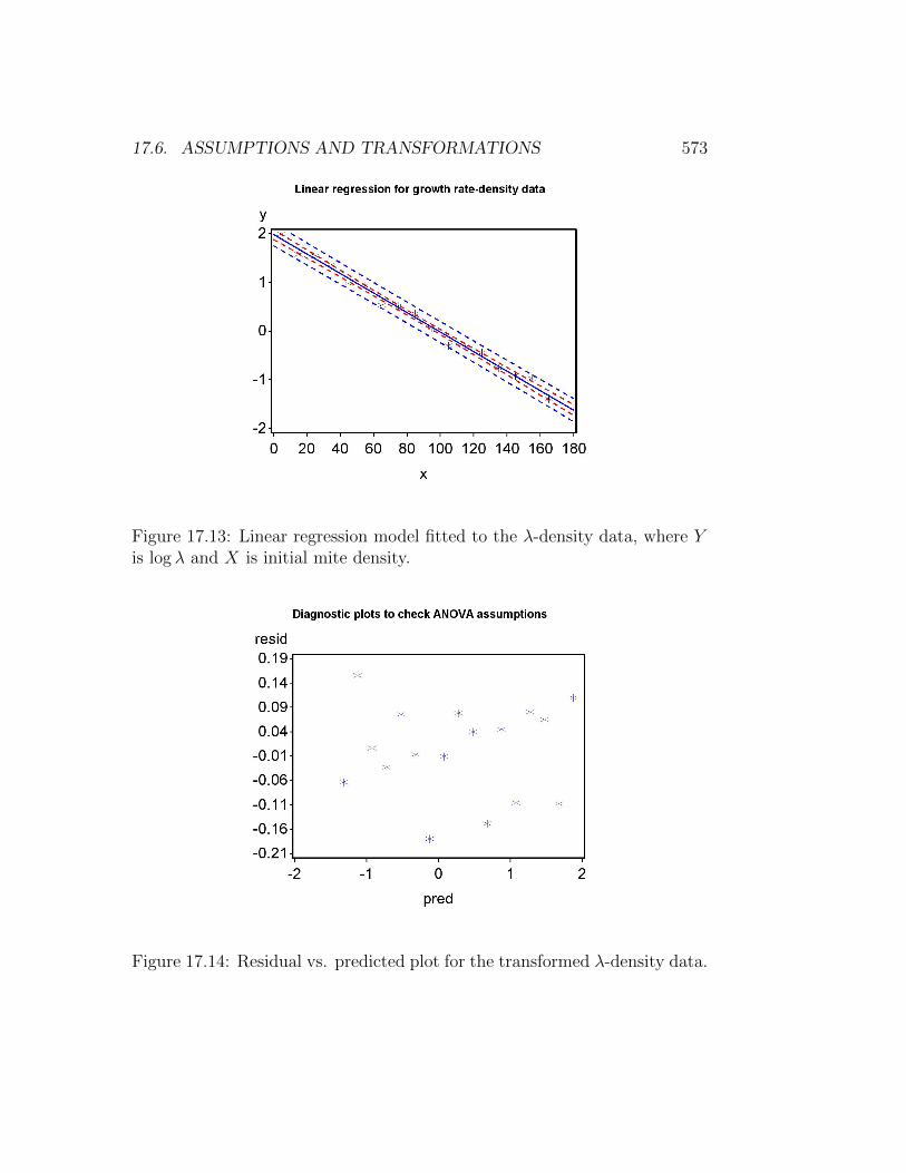
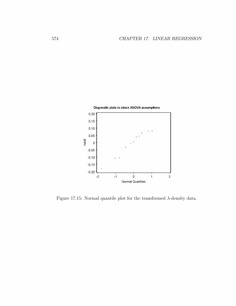
We first conduct the analysis without any transformation. Looking atthe plot of Y (λ) vs. X (density), we see a curvilinear relationship (Fig.17.11) that also appears in the residual vs. predicted plot (Fig. 17.12). Atransformation is clearly needed, but which one? A natural log transforma-tion usually a good starting point for population data, both for growth ratesand numbers. We begin by log-tranforming the dependent variable λ andexamining the plots (see program below). The graph after transformation islinear (Fig. 17.13) and the residual vs. predicted plot shows no pattern (Fig.17.14). The normal quantile plot is also adequate (Fig. 17.15).
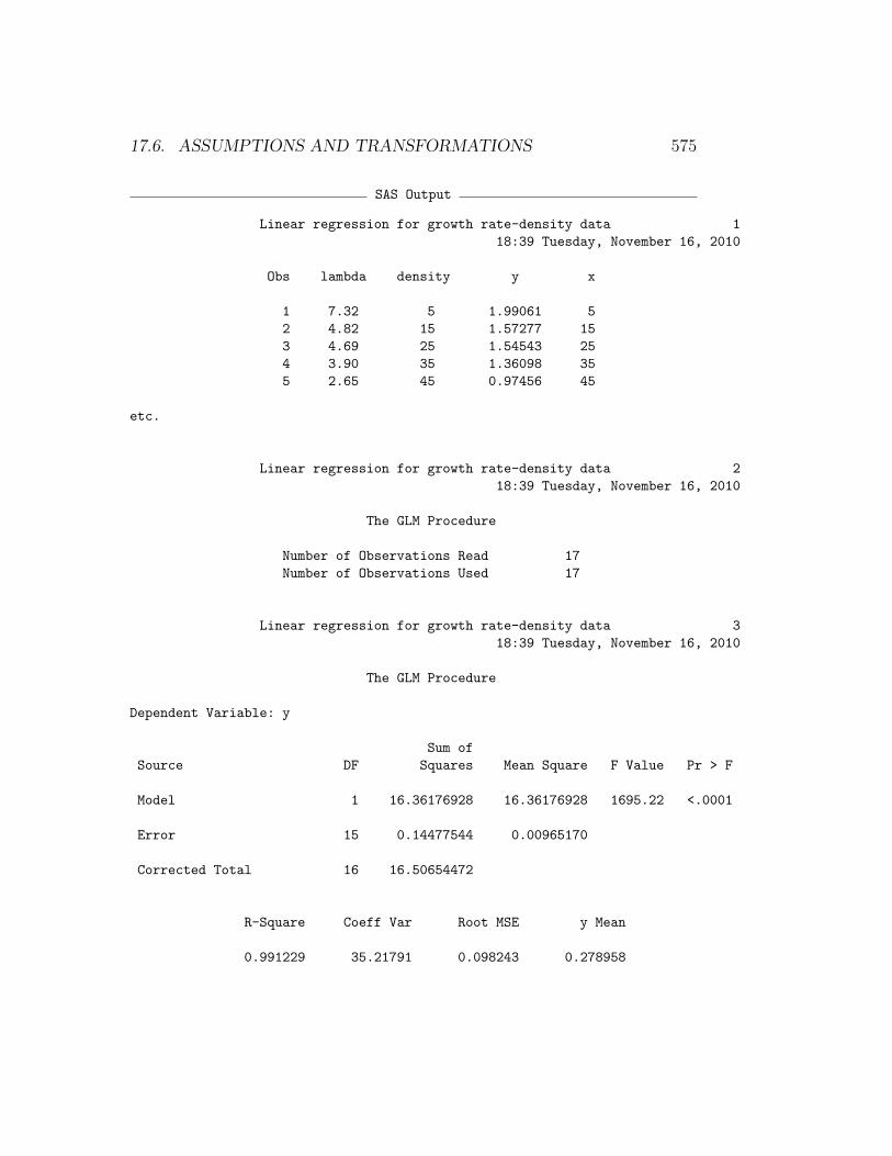
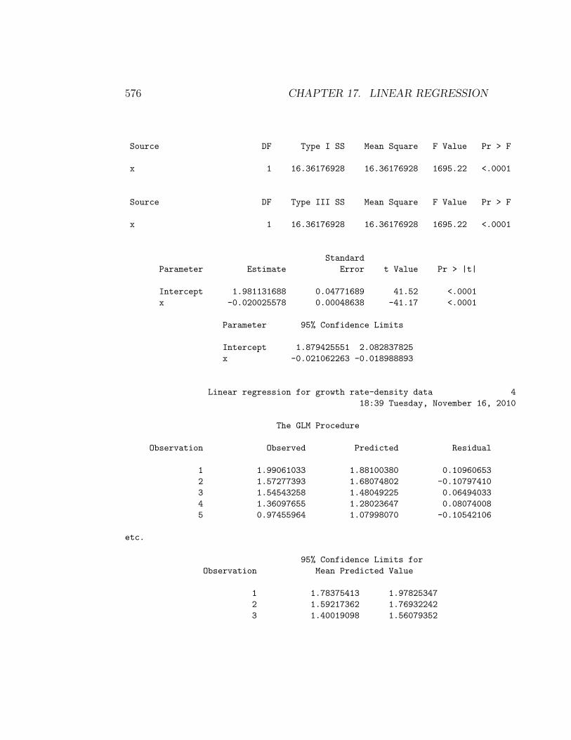
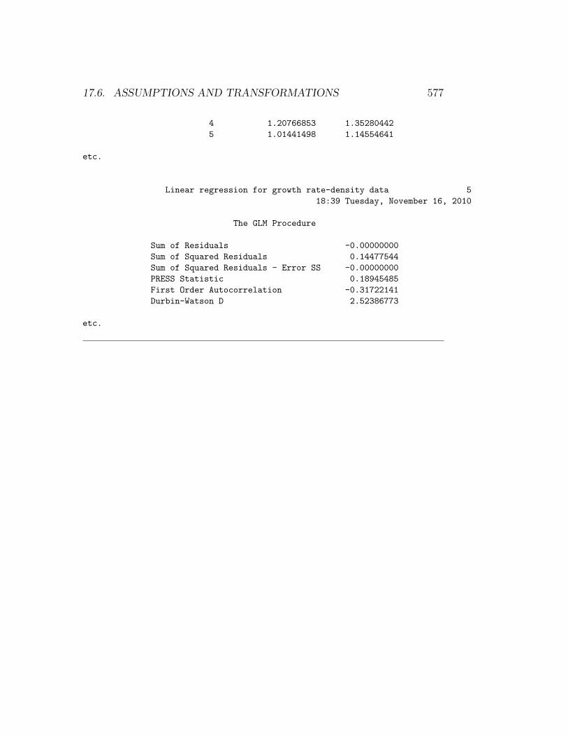
Interpreting the SAS output (see below), we see that λ decreases with mitedensity (β = −0.020) and the effect is highly significant (F1,15 = 1695.22, P <0.0001). The R2 value is 0.991, indicating that almost all the variation in thedata is explained by the regression line. It appears that the growth rate ofthe mites is adversely affected by their density, probably through competitionfor resources or other intraspecific interactions.
570 CHAPTER 17. LINEAR REGRESSION
SAS Program
* logistic.sas;
options pageno=1 linesize=80;
goptions reset=all;
title ’Linear regression for growth rate-density data’;
data grd;
input lambda density;
* Apply transformations here;
y = log(lambda);
x = density;
datalines;
7.32 5
4.82 15
4.69 25
3.90 35
2.65 45
2.52 55
1.70 65
1.68 75
1.43 85
1.07 95
0.74 105
0.72 115
0.64 125
0.47 135
0.40 145
0.38 155
0.25 165
;
run;
* Print data set;
proc print data=grd;
run;
* Plot data and regression line;
proc gplot data=grd;
plot y*x=1 y*x=2 y*x=3 / overlay vaxis=axis1 haxis=axis1;
symbol1 i=none v=star c=black height=2 width=3;
symbol2 i=rlclm v=none c=red height=2 width=3;
symbol3 i=rlcli v=none c=blue height=2 width=3;
axis1 label=(height=2) value=(height=2) width=3 major=(width=2) minor=none;
run;
* Regression analysis with confidence intervals;
proc glm data=grd;
model y = x / clparm clm;
17.6. ASSUMPTIONS AND TRANSFORMATIONS 571
output out=resids p=pred r=resid;
run;
* Regression analysis with prediction intervals;
proc glm data=grd;
model y = x / clparm cli;
run;
goptions reset=all;
title "Diagnostic plots to check ANOVA assumptions";
* Plot residuals vs. predicted values;
proc gplot data=resids;
plot resid*pred=1 / vaxis=axis1 haxis=axis1;
symbol1 v=star height=2 width=3;
axis1 label=(height=2) value=(height=2) width=3 major=(width=2) minor=none;
run;
* Normal quantile plot of residuals;
proc univariate noprint data=resids;
qqplot resid / normal waxis=3 height=4;
run;
quit;
572 CHAPTER 17. LINEAR REGRESSION
Figure 17.11: Linear regression model fitted to the λ-density data, where Yis λ and X is initial mite density.
Figure 17.12: Residual vs. predicted plot for the λ-density data.
17.6. ASSUMPTIONS AND TRANSFORMATIONS 573
Figure 17.13: Linear regression model fitted to the λ-density data, where Yis log λ and X is initial mite density.
Figure 17.14: Residual vs. predicted plot for the transformed λ-density data.
574 CHAPTER 17. LINEAR REGRESSION
Figure 17.15: Normal quantile plot for the transformed λ-density data.
17.6. ASSUMPTIONS AND TRANSFORMATIONS 575
SAS Output
Linear regression for growth rate-density data 1
18:39 Tuesday, November 16, 2010
Obs lambda density y x
1 7.32 5 1.99061 5
2 4.82 15 1.57277 15
3 4.69 25 1.54543 25
4 3.90 35 1.36098 35
5 2.65 45 0.97456 45
etc.
Linear regression for growth rate-density data 2
18:39 Tuesday, November 16, 2010
The GLM Procedure
Number of Observations Read 17
Number of Observations Used 17
Linear regression for growth rate-density data 3
18:39 Tuesday, November 16, 2010
The GLM Procedure
Dependent Variable: y
Sum of
Source DF Squares Mean Square F Value Pr > F
Model 1 16.36176928 16.36176928 1695.22 <.0001
Error 15 0.14477544 0.00965170
Corrected Total 16 16.50654472
R-Square Coeff Var Root MSE y Mean
0.991229 35.21791 0.098243 0.278958
576 CHAPTER 17. LINEAR REGRESSION
Source DF Type I SS Mean Square F Value Pr > F
x 1 16.36176928 16.36176928 1695.22 <.0001
Source DF Type III SS Mean Square F Value Pr > F
x 1 16.36176928 16.36176928 1695.22 <.0001
Standard
Parameter Estimate Error t Value Pr > |t|
Intercept 1.981131688 0.04771689 41.52 <.0001
x -0.020025578 0.00048638 -41.17 <.0001
Parameter 95% Confidence Limits
Intercept 1.879425551 2.082837825
x -0.021062263 -0.018988893
Linear regression for growth rate-density data 4
18:39 Tuesday, November 16, 2010
The GLM Procedure
Observation Observed Predicted Residual
1 1.99061033 1.88100380 0.10960653
2 1.57277393 1.68074802 -0.10797410
3 1.54543258 1.48049225 0.06494033
4 1.36097655 1.28023647 0.08074008
5 0.97455964 1.07998070 -0.10542106
etc.
95% Confidence Limits for
Observation Mean Predicted Value
1 1.78375413 1.97825347
2 1.59217362 1.76932242
3 1.40019098 1.56079352
17.6. ASSUMPTIONS AND TRANSFORMATIONS 577
4 1.20766853 1.35280442
5 1.01441498 1.14554641
etc.
Linear regression for growth rate-density data 5
18:39 Tuesday, November 16, 2010
The GLM Procedure
Sum of Residuals -0.00000000
Sum of Squared Residuals 0.14477544
Sum of Squared Residuals - Error SS -0.00000000
PRESS Statistic 0.18945485
First Order Autocorrelation -0.31722141
Durbin-Watson D 2.52386773
etc.
578 CHAPTER 17. LINEAR REGRESSION
17.7 Problems
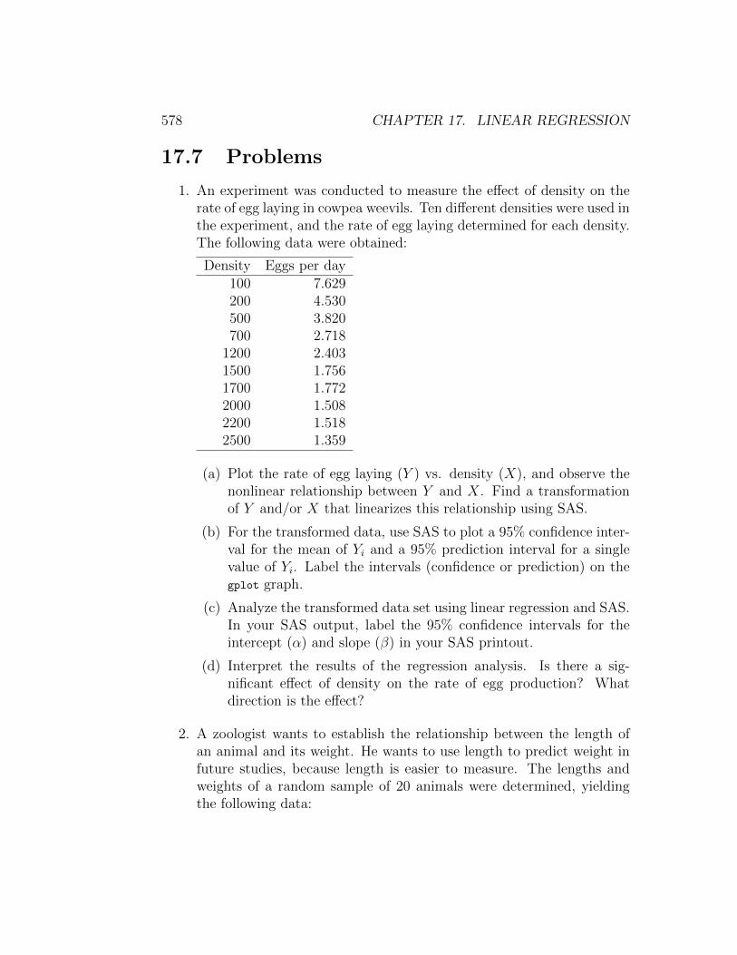
1. An experiment was conducted to measure the effect of density on therate of egg laying in cowpea weevils. Ten different densities were used inthe experiment, and the rate of egg laying determined for each density.The following data were obtained:
Density Eggs per day100 7.629200 4.530500 3.820700 2.718
1200 2.4031500 1.7561700 1.7722000 1.5082200 1.5182500 1.359
(a) Plot the rate of egg laying (Y ) vs. density (X), and observe thenonlinear relationship between Y and X. Find a transformationof Y and/or X that linearizes this relationship using SAS.
(b) For the transformed data, use SAS to plot a 95% confidence inter-val for the mean of Yi and a 95% prediction interval for a singlevalue of Yi. Label the intervals (confidence or prediction) on thegplot graph.
(c) Analyze the transformed data set using linear regression and SAS.In your SAS output, label the 95% confidence intervals for theintercept (α) and slope (β) in your SAS printout.
(d) Interpret the results of the regression analysis. Is there a sig-nificant effect of density on the rate of egg production? Whatdirection is the effect?
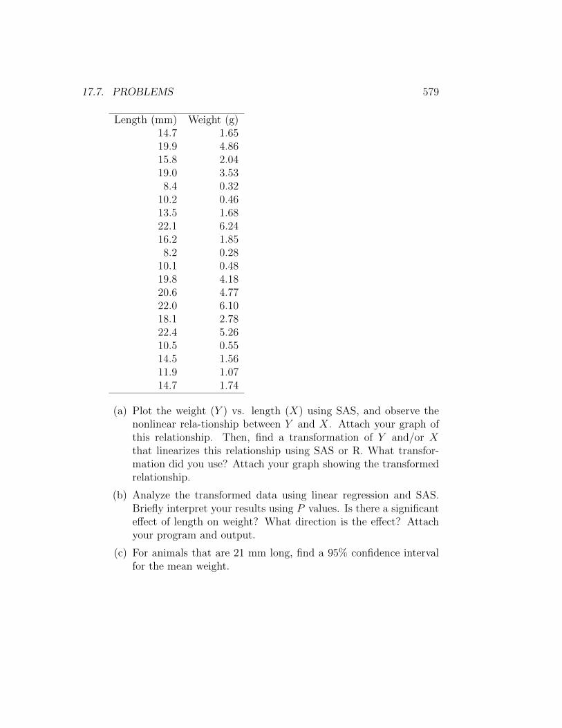
2. A zoologist wants to establish the relationship between the length ofan animal and its weight. He wants to use length to predict weight infuture studies, because length is easier to measure. The lengths andweights of a random sample of 20 animals were determined, yieldingthe following data:
17.7. PROBLEMS 579
Length (mm) Weight (g)14.7 1.6519.9 4.8615.8 2.0419.0 3.538.4 0.32
10.2 0.4613.5 1.6822.1 6.2416.2 1.858.2 0.28
10.1 0.4819.8 4.1820.6 4.7722.0 6.1018.1 2.7822.4 5.2610.5 0.5514.5 1.5611.9 1.0714.7 1.74
(a) Plot the weight (Y ) vs. length (X) using SAS, and observe thenonlinear rela-tionship between Y and X. Attach your graph ofthis relationship. Then, find a transformation of Y and/or Xthat linearizes this relationship using SAS or R. What transfor-mation did you use? Attach your graph showing the transformedrelationship.
(b) Analyze the transformed data using linear regression and SAS.Briefly interpret your results using P values. Is there a significanteffect of length on weight? What direction is the effect? Attachyour program and output.
(c) For animals that are 21 mm long, find a 95% confidence intervalfor the mean weight.
580 CHAPTER 17. LINEAR REGRESSION
17.8 References
MacArthur, R. H. & Wilson, E. O. (1967) The Theory of Island Biogeography.Princeton University Press, Princeton, NJ.
McCulloch, C. E. & Searle, S. R. (2001) Generalized, Linear, and MixedModels. John Wiley & Sons, Inc., New York, NY.
Reeve, J. D., Rhodes, D. J. & Turchin, P. (1998) Scramble competition insouthern pine beetle (Coleoptera: Scolytidae). Ecological Entomology 23:433-443.
SAS Institute Inc. (2014a) SAS/GRAPH 9.4: Reference, Third Edition.SAS Institute Inc., Cary, NC.
SAS Institute Inc. (2014b) SAS/STAT 13.2 Users Guide. SAS Institute Inc.,Cary, NC.
Searle, S. R. (1971) Linear Models. John Wiley & Sons, Inc., New York, NY.
Related Documents