Cg/Stability Map for the Reference H Cycle 3 Supersonic ...mln/ltrs-pdfs/NASA-99-cr209527.pdf · Cg/Stability Map for the Reference H Cycle 3 Supersonic Transport Concept Along the

NASA/CR-1999-209527

Cg/Stability Map for the Reference H Cycle 3Supersonic Transport Concept Along theHigh Speed Research Baseline Mission Profile

Daniel P. Giesy and David M. ChristhilfLockheed Martin Engineering & Sciences Company, Hampton, Virginia

December 1999

The NASA STI Program Office . . . in Profile

Since its founding, NASA has been dedicated

to the advancement of aeronautics and space

science. The NASA Scientific and Technical

Information (STI) Program Office plays a key

part in helping NASA maintain this

important role.

The NASA STI Program Office is operated by

Langley Research Center, the lead center for

NASA’s scientific and technical information.

The NASA STI Program Office provides

access to the NASA STI Database, the

largest collection of aeronautical and space

science STI in the world. The Program Office

is also NASA’s institutional mechanism for

disseminating the results of its research and

development activities. These results are

published by NASA in the NASA STI Report

Series, which includes the following report

types:

• TECHNICAL PUBLICATION. Reports of

completed research or a major significant

phase of research that present the results

of NASA programs and include extensive

data or theoretical analysis. Includes

compilations of significant scientific and

technical data and information deemed

to be of continuing reference value. NASA

counterpart of peer-reviewed formal

professional papers, but having less

stringent limitations on manuscript

length and extent of graphic

presentations.

• TECHNICAL MEMORANDUM.

Scientific and technical findings that are

preliminary or of specialized interest,

e.g., quick release reports, working

papers, and bibliographies that contain

minimal annotation. Does not contain

extensive analysis.

• CONTRACTOR REPORT. Scientific and

technical findings by NASA-sponsored

contractors and grantees.

• CONFERENCE PUBLICATION.

Collected papers from scientific and

technical conferences, symposia,

seminars, or other meetings sponsored or

co-sponsored by NASA.

• SPECIAL PUBLICATION. Scientific,

technical, or historical information from

NASA programs, projects, and missions,

often concerned with subjects having

substantial public interest.

• TECHNICAL TRANSLATION. English-

language translations of foreign scientific

and technical material pertinent to

NASA’s mission.

Specialized services that complement the

STI Program Office’s diverse offerings include

creating custom thesauri, building customized

databases, organizing and publishing

research results . . . even providing videos.

For more information about the NASA STI

Program Office, see the following:

• Access the NASA STI Program Home

Page at http://www.sti.nasa.gov

• Email your question via the Internet to

[email protected]

• Fax your question to the NASA STI

Help Desk at (301) 621-0134

• Telephone the NASA STI Help Desk at

(301) 621-0390

• Write to:

NASA STI Help Desk

NASA Center for AeroSpace Information

7121 Standard Drive

Hanover, MD 21076-1320

NASA/CR-1999-209527

Cg/Stability Map for the Reference H Cycle 3Supersonic Transport Concept Along the HighSpeed Research Baseline Mission Profile

Daniel P. Giesy and David M. ChristhilfLockheed Martin Engineering & Sciences Company, Hampton, Virginia

National Aeronautics and

Space Administration

Langley Research Center

Hampton, Virginia 23681-2199

Prepared for Langley Research Center

under Contract NAS1-96014

December 1999

Available from:

NASA Center for AeroSpace Information (CASI) National Technical Information Service (NTIS)

7121 Standard Drive 5285 Port Royal Road

Hanover, MD 21076-1320 Springfield, VA 22161-2171

(301) 621-0390 (703) 605-6000

Abstract

A comparison is made between the results of trimming a High Speed Civil Transport (H-SCT) concept along a reference mission profile using two trim modes. One mode uses thestabilator. The other mode uses fore and aft placement of the center of gravity. A comparisonis made of the throttle settings (cruise segments) or the total acceleration (ascent and descentsegments) and of the drag coefficient. The comparative stability of trimming using the twomodes is also assessed by comparing the stability margins and the placement of the lateral andlongitudinal eigenvalues.

IntroductionThe study reported in this document is a follow on study to the work reported by Chowdhry

and Buttrill in their memorandum [1]. In that report, they documented “a study performed toassess the bare airframe stability characteristics of a HSCT configuration and to investigate thebenefits, if any, of using an active fuel management system to reduce trim drag.” The study consistsof trimming the aircraft at each point along a reference mission profile (1) holding the x-cg atits nominal position and using the stabilator and (2) holding the stabilator at zero deflection andmoving the x-cg to trim. Stability and performance measures of the aircraft are compared at thetwo trim conditions at each point of the reference mission profile.

Ref. [1] studied the Reference H, cycle 1 HSCT concept. The present study uses theReference H Cycle 3 airplane (Ref. H-3) [2].

Reference Mission ProfileThe reference mission profile was taken from a TCA Configuration Description Document

[3, pp. A32 – A43]. It is described by a sample of 79 flight conditions divided into five segments:

Seg. 1Climb, 30 flight conditions (numbers 1 – 30).

Seg. 2Supersonic cruise, 13 flight conditions (numbers 31 – 43).

Seg. 3Supersonic descent, 16 flight conditions (numbers 44 – 59).

Seg. 4Subsonic cruise, 13 flight conditions (numbers 60 – 72).

Seg. 5Subsonic descent, 7 flight conditions (numbers 73 – 79).

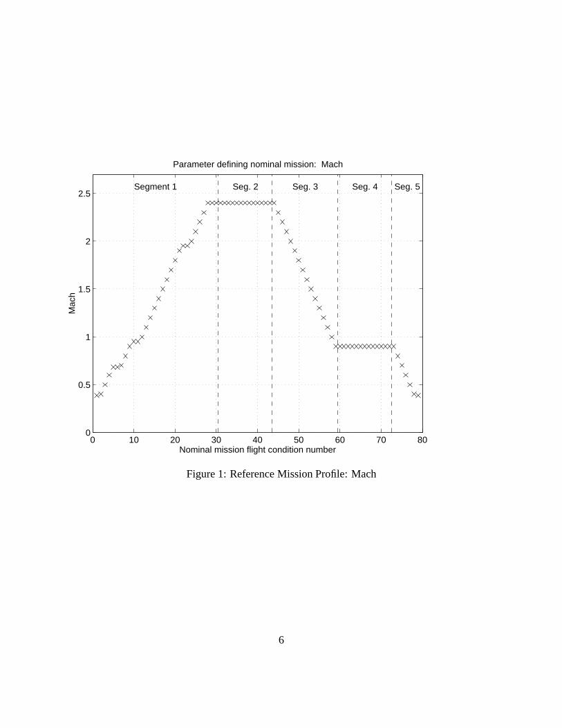
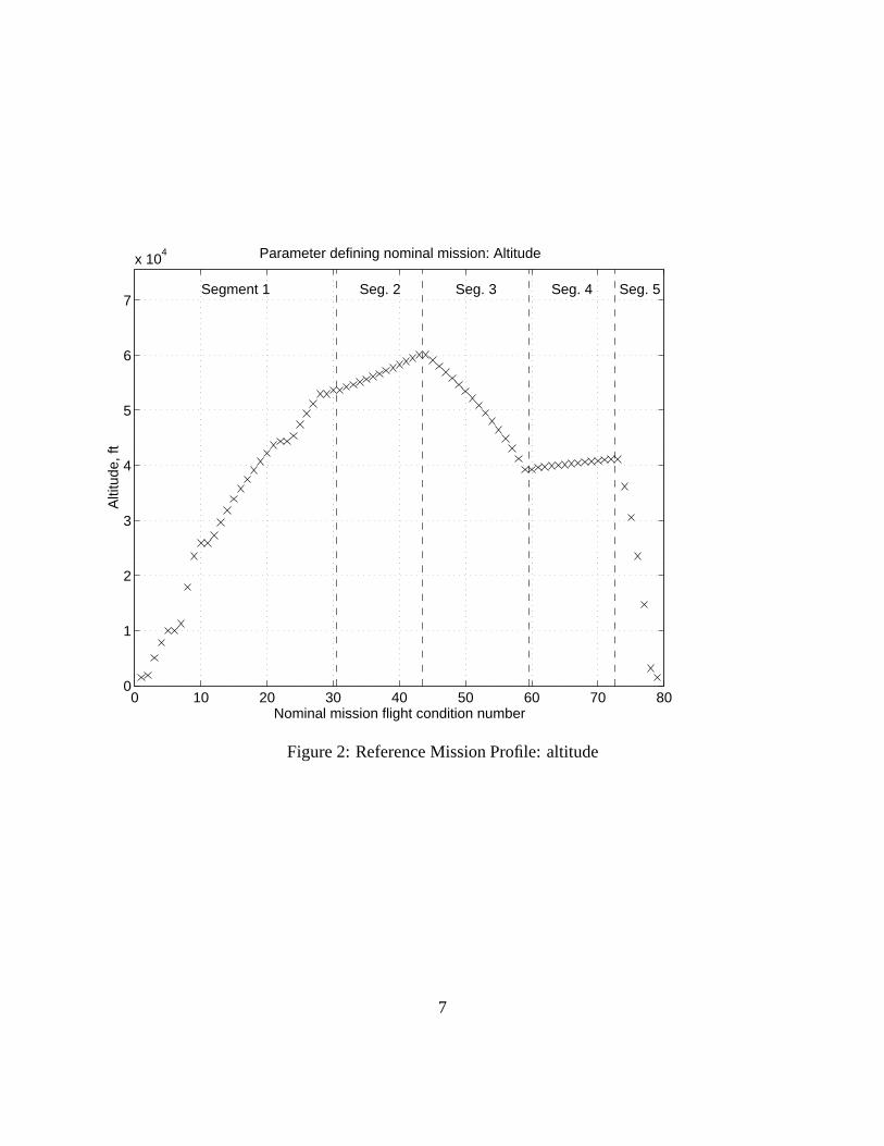
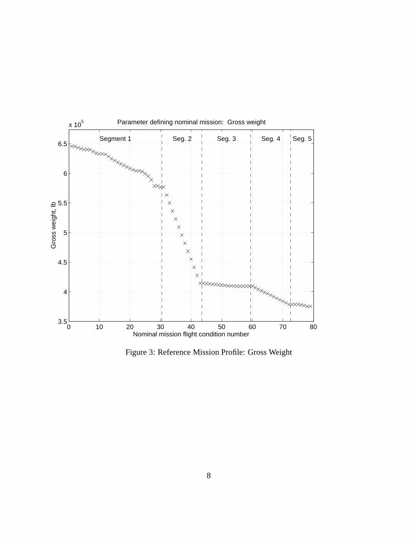
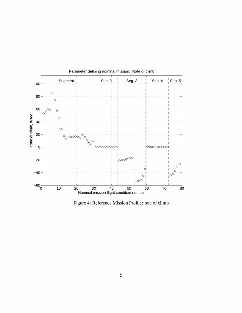
This mission profile was designed for the Technology Concept Airplane (TCA) which isheavier than Ref. H-3. To correct for this weight differential, the aircraft weights from the TCAmission profile have been multiplied by the factor 649914/740600 which is the ratio of the maxi-mum taxi weight of Ref. H-3 to that of TCA. Each flight condition of the reference mission profileis then defined by its Mach number, its altitude, its (scaled) weight, and its rate of climb. These areshown in Figs. 1 – 4.

Modeling and Analysis SoftwareThe model of Ref. H-3 and much of the analysis software was contained in an integrated

MATLAB/SIMULINK HSCT simulation [4]. The software modulerefhsim3 trim.m in [4]performed an analysis of the Ref. H-3 aircraft at each flight condition using specific values ofthe trim variables. For this analysis, the AUTOCGFLAG and the AUTOWTFLAG were turnedoff; weight was scheduled by the reference mission profile as already explained and the center

2

of gravity was determined by interpolation using the five standard mass sets as explained in thenext section. The AUTOFLAPFLAG was on, so that flaps followed their automatic schedule, andRIGID FLAG was off, so Quasi-Steady AeroElastic (QSAE) increments were incorporated. TheMATLAB Optimization Toolbox constrained optimization routineconstr.m was used to varythe trim variables to achieve the trim conditions. Once trim was achieved, the derivatives@CM=@�and@CL=@� were estimated using a central difference derivative approximation with�� = :1deg., further utilizingrefhsim3 trim.m . Stability margin (as a per cent of mean aerodynamicchord) was then calculated to be�100(@CM=@�)=(@CL=@�).

The trimmed aircraft was then linearized usinglinearmodel.m and refh-sim3 lin.m from [4]. Lateral and longitudinal eigenvalues were calculated by applying MAT-LAB built-in function eig to subblocks of the linear system matrix.

Trim DetailsIn all trim runs, the thrust multiplier was set to 1.09, so that maximum power available

was 109% of nominal maximum. This was suggested by Dr. Chris Gracey of LaRC based on hisexperience with calculating fuel optimal trajectories.

At all flight conditions, nominal X and Z positions of the center of gravity were determinedby linear interpolation using gross weight as the independent variable and using the simulationmass sets from [2, Table 3.1-1, Page 3-2]. The relevant data are (Z-CG data come from a Boeing-supplied FORTRAN subroutineDATAstatement):

Mass Set Gross Weight (lb) XCG BS(in) ZCG WL(in)M01 279,080 2153.5 201.50MFC 384,862 2139.2 207.46MCR 501,324 2155.7 203.15MIC 614,864 2132.2 200.59M13 649,914 2086.0 199.56

At each flight condition, the aircraft was trimmed in two different ways. In theStabilatortrimmedcase, the X-CG was held at its nominal value, and trim was achieved using the coupledstabilizer and elevator (withDELEV1 = DELEV2 = 2*DSTAB). In theCG trimmedcase, thestabilator was held at 0 degrees deflection, and the X-CG was moved to achieve trim.

In all trim cases the body axis X-velocity,u, the body axis Z-velocity,w, and the Euler pitchangle,�, were used as trim variables. The parameters gross weight and altitude were scheduled bythe flight condition.

In all trim cases, the trim constraints included constant angle of attack (_� = 0) and constantpitch rate (_q = 0). Mach and rate of climb were constrained to values scheduled by flight condition.

During climb (Seg. 1), throttle was set to max (100%) and during descent (Segs. 3 and 5),throttle was set to idle (3%). During the cruise segments (Segs. 2 and 4), an additional constraintwas imposed; total velocity was to be constant (_VT = 0). The throttle setting then became anadditional trim variable.

After trim was calculated, the stability margin was determined as previously noted. Thetrimmed aircraft was then linearized. The linearized states are:

1. Total Velocity,VT ,

3

2. Angle-of-attack,�,

3. Pitch rate,q,

4. Euler angle�,

5. Altitude,h,

6. Roll rate,p,

7. Yaw rate,r,

8. Bank angle�,

9. Sidslip angle�,

10. Euler angle ,

11. Latitude, and

12. Longitude.

Linearization of the trimmed aircraft produces a 12 by 12 state matrix,A. The longitudinaleigenvalues are found by taking the eigenvalues of the sub-matrix ofA consisting of the first 5 rowsand columns ofA. The lateral eigenvalues are found by taking the eigenvalues of the sub-matrixof A consisting of rows and columns 6 – 9 ofA.

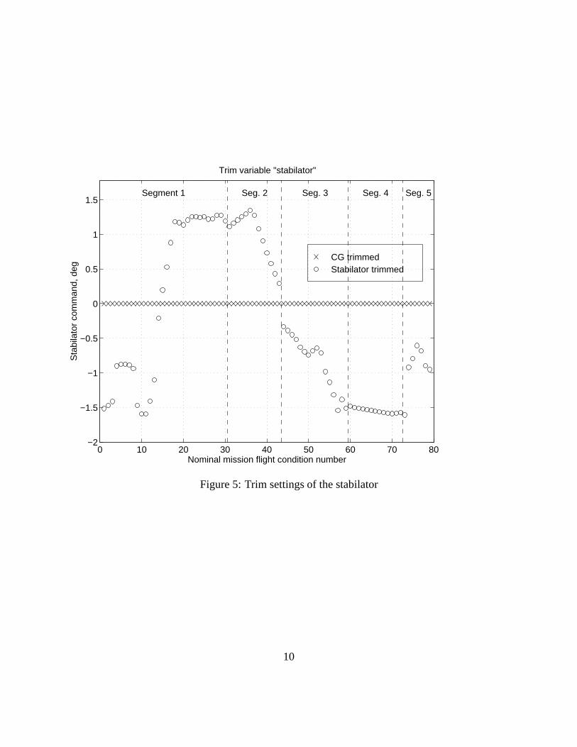
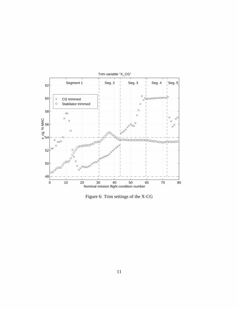
Trim ResultsTrim values of trim variables are shown in Figs. 5 – 10. Fig. 5 shows that, with the X-CG

held to its nominal position, trim can be established throughout the reference mission profile withstabilizer deflections of no more than about�1:5Æ (with coupled elevator deflections of up to about�3Æ). Fig. 6 shows the nominal X-CG schedule (circles) and the X-CG position needed to trim inthe absence of stabilator deflection (x’s). The horizontal dash-dot lines show the forward (48%)and aft (54%) X-CG limits as given in [2, Page B-8]. The nominal X-CG schedule takes it outsidethese limits during part of the supersonic cruise segment (Seg. 2). The trim position of the X-CG,however, exceeds the aft X-CG limit both more often and by a greater amount than the nominal.The elapsed time to fly from flight condition 8 to 15 (the last condition before the X-CG exceedsits aft limit until the first condition where the X-CG has returned to its limit) is 10 minutes 22seconds. Besides the question of whether one would want to exceed the limit by so much, there isthe question of whether one would want to include high enough capacity fuel pumping systems tomove the X-CG that rapidly. The X-CG trim position throughout the entire descent and subsoniccruise phase (Segs. 3 – 5) falls outside the aft limit, the excess becoming as much as 6% of meanaerodynamic chord.

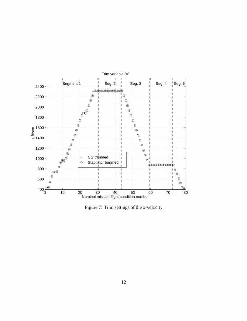
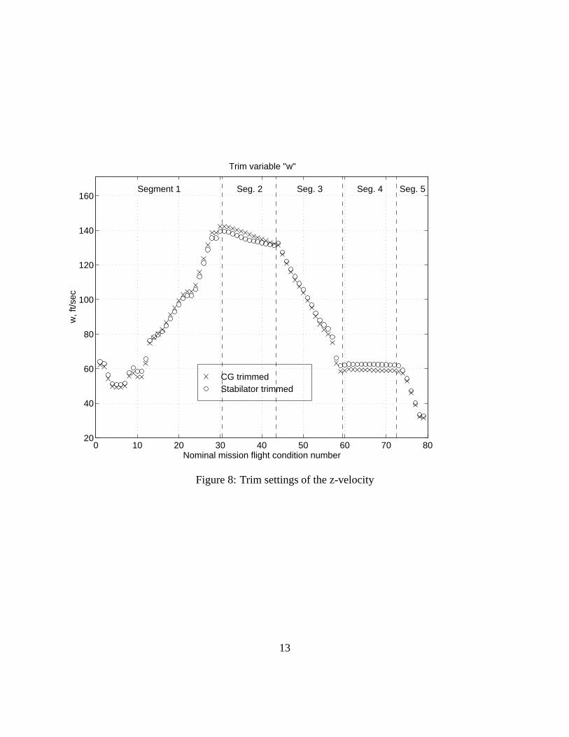
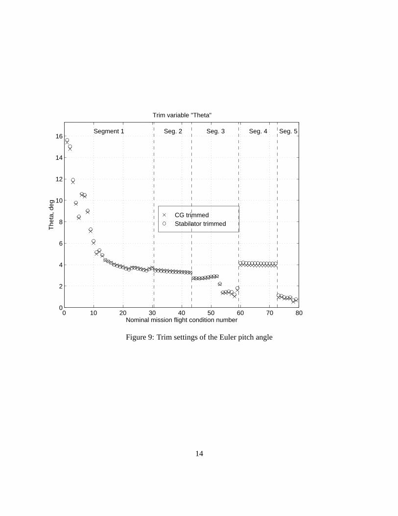
The value of trim variableu to trim the aircraft is shown in Fig. 7. It seems to be quiteinsensitive to whether the aircraft is trimmed by stabilator deflection or X-CG positioning. Thevalues of trim variablesw and�, shown in Figs. 8 and 9, show only slightly more sensitivity to thetrim mode.

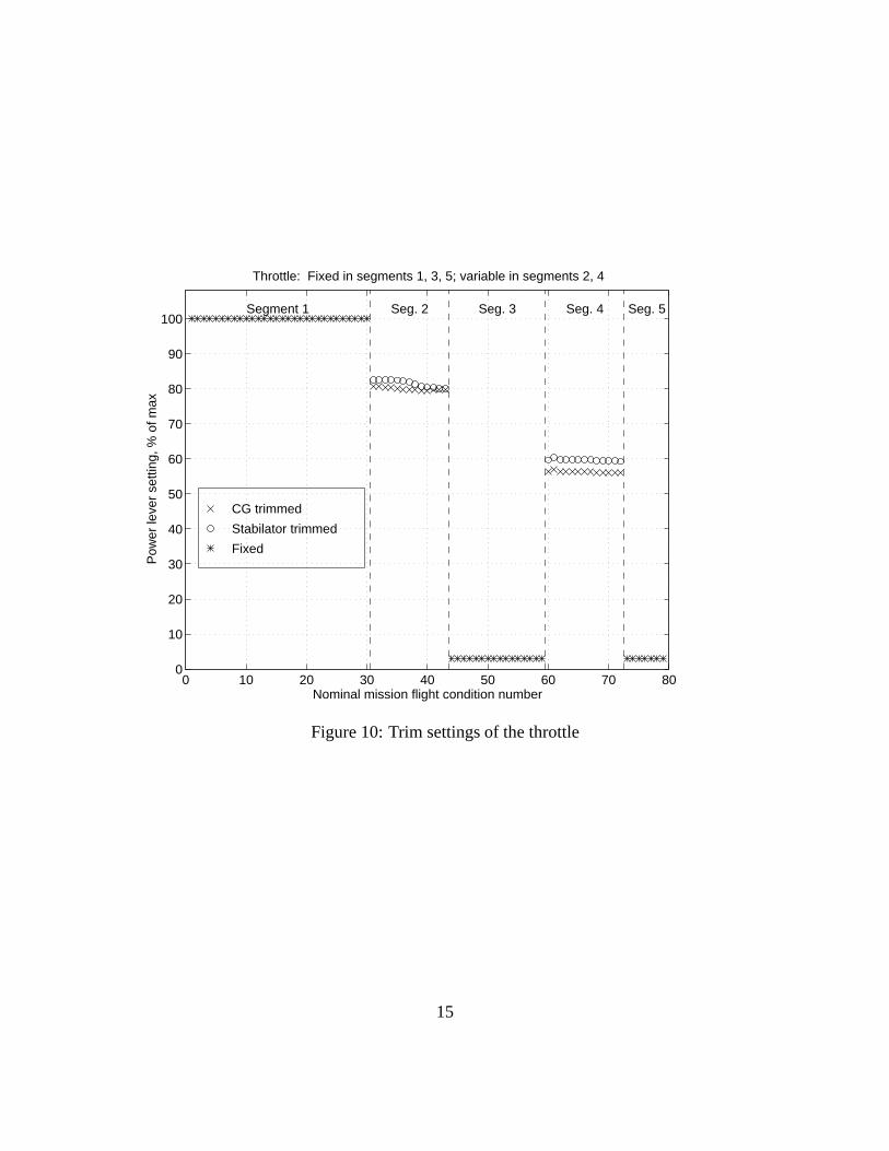
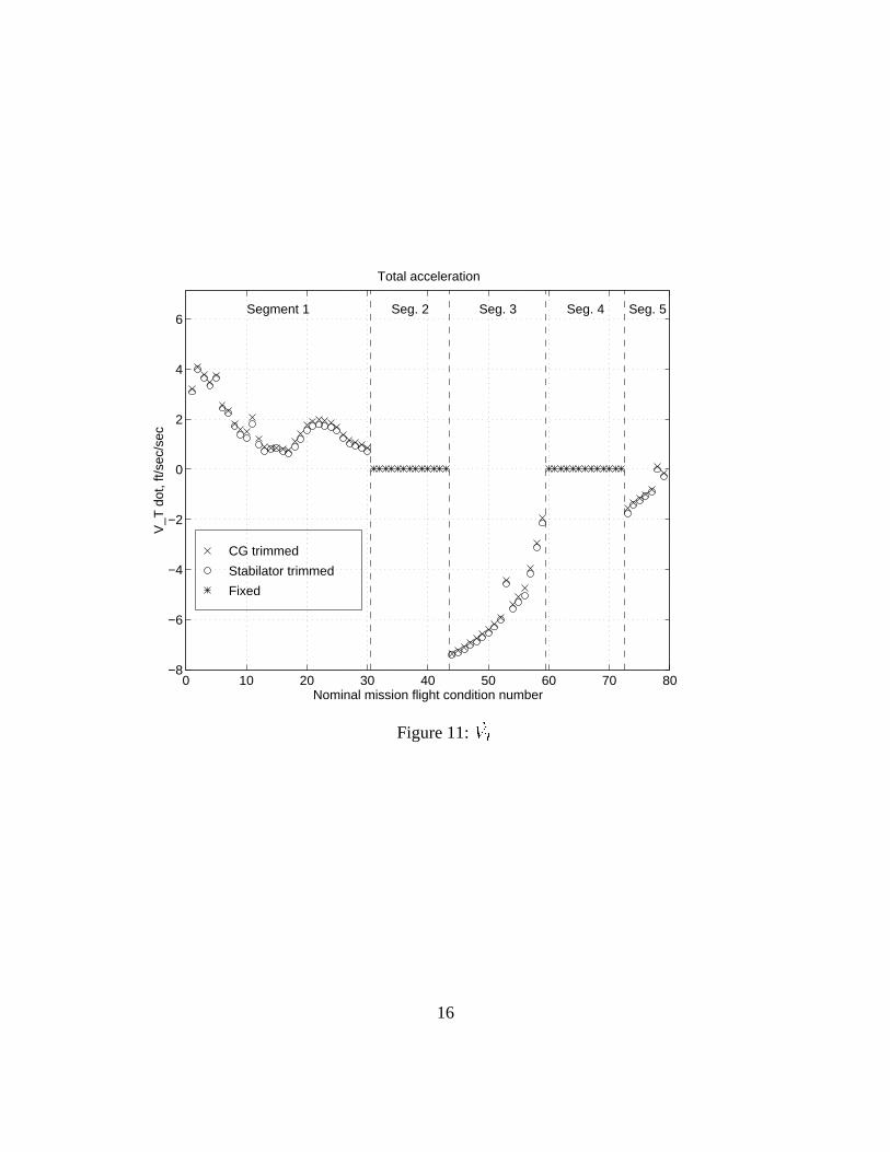
In the cruise segments, the power lever setting is used as an additional trim variable, sup-plemented by adding the constraint that the total acceleration should be zero (_VT = 0). Fig. 10

4

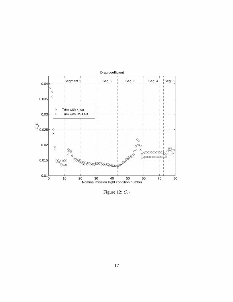
shows that the X-CG trimmed aircraft uses slightly less power in these segments. In the climb anddescent segments, Segs 1, 3, and 5, where the power setting is programmed to a fixed setting, theX-CG trimmed aircraft experiences slightly more acceleration (Fig. 11). Both of these phenomenaare attributable to the reduction in drag coefficient,CD, which is the result of trimming by varyingthe X-CG position as opposed to using the stabilator. This is shown in Fig. 12.

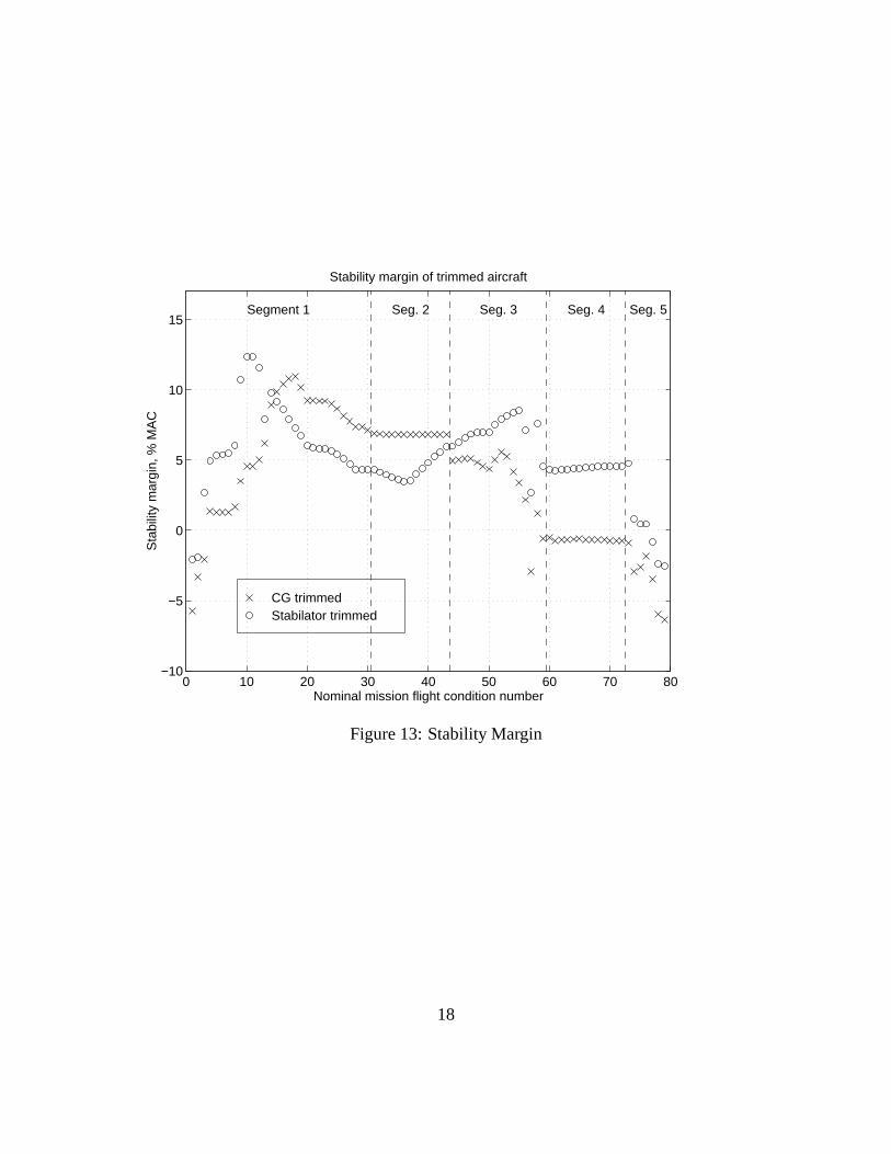
Stability ResultsStability margins for each trimmed condition are shown in Fig. 13. Although the results

between the two trim paradigms are mixed over the reference mission profile, the X-CG trimmedcase seems to have more tendency to go to a negative stability margin than the stabilator trimmedcase.

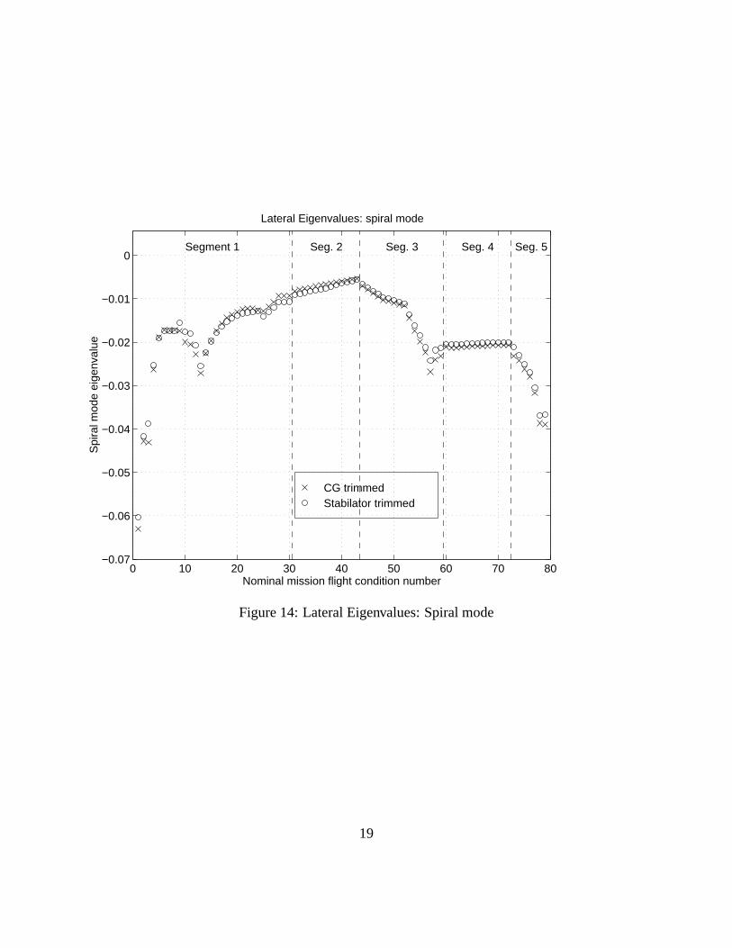
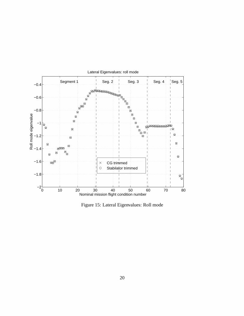
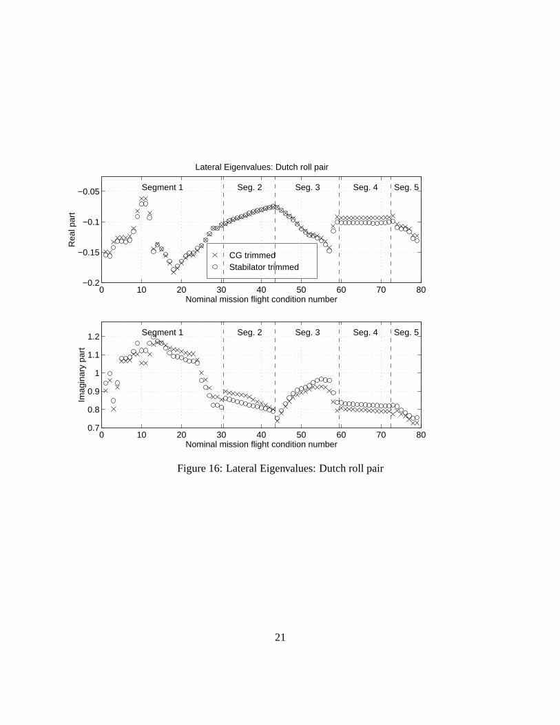
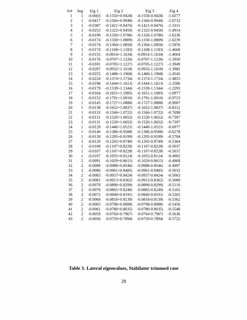
The lateral eigenvalues are well behaved, considerately separating into the conventionalspiral mode, roll mode, and Dutch roll pair. The spiral mode remains stable (Fig. 14), as doesthe roll mode which is shown in Fig. 15 and the Dutch roll pair whose real and imaginary partsare plotted as a function of flight condition number in Fig. 16. Dutch roll damping also seemsadequate.

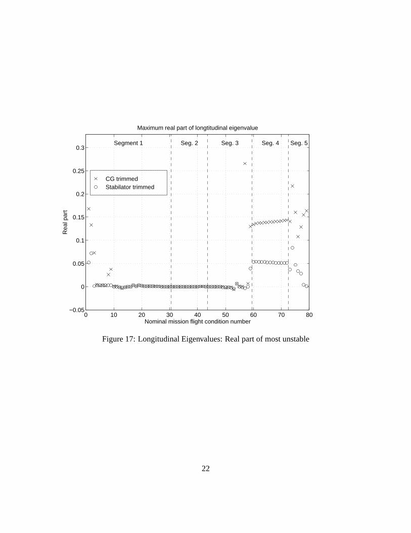
The longitudinal eigenvalues were not so readily identifiable. Fig. 17 shows the real partof the most unstable longitudinal eigenvalue. Fig. 18 gives a scatter plot of all the longitudinaleigenvalues with the two trim paradigms plotted separately. The raw eigenvalue data are tabulatedat the end of this report.

AcknowledgementThe authors are grateful to Dr. Christopher Gracey of NASA Langley Research Center for

his help in locating data for this study and in formulating the approach.

References

[1] Rajiv Singh Chowdhry and Carey Buttrill, “Reference-H Assessment: Bare Airframe Stabilityand Trim Drag Reduction,” Memo to GFC ITD, September 13, 1995.

[2] “High Speed Civil Transport Reference H – Cycle 3 Simulation Data Base.” A Boeing reportfor NASA Contract NAS1-20220, Task Assignment No. 36, WBS 4.3.5.1.2.1.

[3] “High Speed Research Program HSR II – Airframe task 20; Task 2.1 – Technology Integration;Sub-task 2.1.1.1 Refine Technology Concept Airplane: Configuration Description Document;Deliverable Report.” Approved by J. B. Coffey, BCAG; J. K. Wechsler, MDC; P. F. Sweetland,BCAG; H. R. Welge, MDC. Prepared for NASA Langley Research Center, NASA ContractNAS1-20220. April 1, 1996.

[4] Rajiv S. Chowdhry, “User’s Manual for MATLAB ReferenceH Cycle 3 Simulation Software”,December, 1996.

5

0 10 20 30 40 50 60 70 800

0.5

1

1.5

2

2.5

Nominal mission flight condition number

Mac

h

Parameter defining nominal mission: Mach

Segment 1 Seg. 2 Seg. 3 Seg. 4 Seg. 5

Figure 1: Reference Mission Profile: Mach

6

0 10 20 30 40 50 60 70 800

1

2

3

4

5

6

7

x 104


Alti

tude

, ft

Parameter defining nominal mission: Altitude


Figure 2: Reference Mission Profile: altitude

7

0 10 20 30 40 50 60 70 803.5

4

4.5

5

5.5

6

6.5

x 105


Gro

ss w

eigh

t, lb

Parameter defining nominal mission: Gross weight


Figure 3: Reference Mission Profile: Gross Weight

8

0 10 20 30 40 50 60 70 80−60

−40

−20

0

20

40

60

80

100


Rat

e of

clim

b, ft

/sec

Parameter defining nominal mission: Rate of climb


Figure 4: Reference Mission Profile: rate of climb

9

CG trimmed Stabilator trimmed

0 10 20 30 40 50 60 70 80−2

−1.5

−1

−0.5

0

0.5

1

1.5


Sta

bila

tor

com

man

d, d

eg

Trim variable "stabilator"


Figure 5: Trim settings of the stabilator

10


0 10 20 30 40 50 60 70 80

48

50

52

54

56

58

60

62


x_cg

, % M

AC

Trim variable "X_CG"


Figure 6: Trim settings of the X-CG

11


0 10 20 30 40 50 60 70 80400

600

800

1000

1200

1400

1600

1800

2000

2200

2400


u, ft

/sec

Trim variable "u"


Figure 7: Trim settings of the x-velocity

12


0 10 20 30 40 50 60 70 8020

40

60

80

100

120

140

160


w, f

t/sec

Trim variable "w"


Figure 8: Trim settings of the z-velocity

13


0 10 20 30 40 50 60 70 800

2

4

6

8

10

12

14

16


The

ta, d

eg

Trim variable "Theta"


Figure 9: Trim settings of the Euler pitch angle

14

CG trimmed

Stabilator trimmed

Fixed

0 10 20 30 40 50 60 70 800

10

20

30

40

50

60

70

80

90

100


Pow

er le

ver

setti

ng, %

of m

ax

Throttle: Fixed in segments 1, 3, 5; variable in segments 2, 4


Figure 10: Trim settings of the throttle

15

CG trimmed

Stabilator trimmed

Fixed

0 10 20 30 40 50 60 70 80−8

−6

−4

−2

0

2

4

6


V_T

dot

, ft/s

ec/s

ec

Total acceleration


Figure 11: _VT

16

Trim with x_cg Trim with DSTAB

0 10 20 30 40 50 60 70 800.01

0.015

0.02

0.025

0.03

0.035

0.04


C_D

Drag coefficient


Figure 12:CD

17


0 10 20 30 40 50 60 70 80−10

−5

0

5

10

15


Sta

bilit

y m

argi

n, %

MA

C

Stability margin of trimmed aircraft


Figure 13: Stability Margin

18


0 10 20 30 40 50 60 70 80−0.07

−0.06

−0.05

−0.04

−0.03

−0.02

−0.01

0


Spi

ral m

ode

eige

nval

ue

Lateral Eigenvalues: spiral mode


Figure 14: Lateral Eigenvalues: Spiral mode

19


0 10 20 30 40 50 60 70 80−2

−1.8

−1.6

−1.4

−1.2

−1

−0.8

−0.6

−0.4


Rol

l mod

e ei

genv

alue

Lateral Eigenvalues: roll mode


Figure 15: Lateral Eigenvalues: Roll mode

20


0 10 20 30 40 50 60 70 80−0.2

−0.15

−0.1

−0.05


Rea

l par

t

Lateral Eigenvalues: Dutch roll pair


0 10 20 30 40 50 60 70 800.7

0.8

0.9

1

1.1

1.2


Imag

inar

y pa

rt


Figure 16: Lateral Eigenvalues: Dutch roll pair

21


0 10 20 30 40 50 60 70 80−0.05

0

0.05

0.1

0.15

0.2

0.25

0.3


Rea

l par

t

Maximum real part of longtitudinal eigenvalue


Figure 17: Longitudinal Eigenvalues: Real part of most unstable

22

−1.6 −1.4 −1.2 −1 −0.8 −0.6 −0.4 −0.2 0 0.2 0.4−2

−1

0

1

2

Real part

Imag

inar

y pa

rt

Longitudinal eigenvalues, CG trimmed

−1.5 −1 −0.5 0 0.5−2

−1

0

1

2

Real part

Imag

inar

y pa

rt

Longitudinal eigenvalues, Stabilator trimmed

Figure 18: Longitudinal Eigenvalues: All

23

fc# Seg Eig 1 Eig 2 Eig 3 Eig 41 1 -0.0630 -0.1493+0.9023i -0.1493-0.9023i -1.03352 1 -0.0428 -0.1509+0.9580i -0.1509-0.9580i -1.08043 1 -0.0431 -0.1329+0.8018i -0.1329-0.8018i -1.33924 1 -0.0264 -0.1265+0.9223i -0.1265-0.9223i -1.49565 1 -0.0188 -0.1260+1.0645i -0.1260-1.0645i -1.62326 1 -0.0173 -0.1264+1.0663i -0.1264-1.0663i -1.62357 1 -0.0173 -0.1239+1.0697i -0.1239-1.0697i -1.59728 1 -0.0172 -0.1106+1.1023i -0.1106-1.1023i -1.46599 1 -0.0174 -0.0827+1.1024i -0.0827-1.1024i -1.4031

10 1 -0.0200 -0.0618+1.0538i -0.0618-1.0538i -1.391511 1 -0.0205 -0.0616+1.0540i -0.0616-1.0540i -1.391412 1 -0.0228 -0.0863+1.1031i -0.0863-1.1031i -1.393913 1 -0.0271 -0.1442+1.1536i -0.1442-1.1536i -1.449914 1 -0.0226 -0.1365+1.1651i -0.1365-1.1651i -1.484715 1 -0.0196 -0.1452+1.1675i -0.1452-1.1675i -1.359016 1 -0.0174 -0.1559+1.1521i -0.1559-1.1521i -1.230217 1 -0.0157 -0.1683+1.1366i -0.1683-1.1366i -1.099018 1 -0.0144 -0.1831+1.1271i -0.1831-1.1271i -0.973919 1 -0.0136 -0.1761+1.1244i -0.1761-1.1244i -0.902720 1 -0.0130 -0.1680+1.1181i -0.1680-1.1181i -0.833621 1 -0.0125 -0.1591+1.1091i -0.1591-1.1091i -0.772822 1 -0.0122 -0.1544+1.1038i -0.1544-1.1038i -0.742923 1 -0.0122 -0.1544+1.1038i -0.1544-1.1038i -0.742924 1 -0.0125 -0.1472+1.0714i -0.1472-1.0714i -0.698425 1 -0.0128 -0.1399+1.0004i -0.1399-1.0004i -0.632426 1 -0.0118 -0.1304+0.9612i -0.1304-0.9612i -0.583227 1 -0.0107 -0.1208+0.9172i -0.1208-0.9172i -0.541428 1 -0.0094 -0.1110+0.8687i -0.1110-0.8687i -0.509129 1 -0.0093 -0.1110+0.8687i -0.1110-0.8687i -0.509130 1 -0.0094 -0.1059+0.8542i -0.1059-0.8542i -0.494931 2 -0.0082 -0.1036+0.8968i -0.1036-0.8968i -0.500232 2 -0.0079 -0.0996+0.8916i -0.0996-0.8916i -0.503033 2 -0.0076 -0.0970+0.8875i -0.0970-0.8875i -0.506634 2 -0.0074 -0.0946+0.8835i -0.0946-0.8835i -0.509735 2 -0.0071 -0.0924+0.8794i -0.0924-0.8794i -0.512336 2 -0.0069 -0.0902+0.8753i -0.0902-0.8753i -0.514437 2 -0.0066 -0.0876+0.8674i -0.0876-0.8674i -0.519638 2 -0.0064 -0.0851+0.8535i -0.0851-0.8535i -0.528839 2 -0.0062 -0.0828+0.8427i -0.0828-0.8427i -0.538040 2 -0.0060 -0.0806+0.8320i -0.0806-0.8320i -0.547041 2 -0.0058 -0.0787+0.8213i -0.0787-0.8213i -0.555842 2 -0.0056 -0.0769+0.8103i -0.0769-0.8103i -0.564343 2 -0.0054 -0.0754+0.7999i -0.0754-0.7999i -0.5730

Table 1. Lateral eigenvalues, CG-trimmed case

24

fc# Seg Eig 1 Eig 2 Eig 3 Eig 444 3 -0.0070 -0.0762+0.7364i -0.0762-0.7364i -0.568345 3 -0.0079 -0.0809+0.7791i -0.0809-0.7791i -0.598346 3 -0.0087 -0.0856+0.8147i -0.0856-0.8147i -0.629647 3 -0.0094 -0.0902+0.8439i -0.0902-0.8439i -0.661748 3 -0.0103 -0.0951+0.8664i -0.0951-0.8664i -0.696849 3 -0.0105 -0.1024+0.8804i -0.1024-0.8804i -0.753750 3 -0.0110 -0.1097+0.8895i -0.1097-0.8895i -0.810151 3 -0.0113 -0.1152+0.8994i -0.1152-0.8994i -0.870452 3 -0.0116 -0.1203+0.9095i -0.1203-0.9095i -0.930053 3 -0.0144 -0.1214+0.9226i -0.1214-0.9226i -0.997754 3 -0.0174 -0.1231+0.9220i -0.1231-0.9220i -1.059455 3 -0.0199 -0.1271+0.9247i -0.1271-0.9247i -1.113656 3 -0.0224 -0.1325+0.9218i -0.1325-0.9218i -1.157957 3 -0.0268 -0.1425+0.9011i -0.1425-0.9011i -1.206458 3 -0.0240 -0.1075+0.8418i -0.1075-0.8418i -1.148659 3 -0.0232 -0.0920+0.7933i -0.0920-0.7933i -1.066360 4 -0.0210 -0.0939+0.8088i -0.0939-0.8088i -1.065061 4 -0.0214 -0.0941+0.8009i -0.0941-0.8009i -1.050762 4 -0.0213 -0.0940+0.8000i -0.0940-0.8000i -1.051863 4 -0.0212 -0.0941+0.7989i -0.0941-0.7989i -1.052464 4 -0.0211 -0.0941+0.7978i -0.0941-0.7978i -1.053165 4 -0.0210 -0.0941+0.7967i -0.0941-0.7967i -1.053866 4 -0.0209 -0.0941+0.7957i -0.0941-0.7957i -1.054567 4 -0.0208 -0.0941+0.7941i -0.0941-0.7941i -1.055268 4 -0.0208 -0.0941+0.7924i -0.0941-0.7924i -1.056069 4 -0.0208 -0.0941+0.7907i -0.0941-0.7907i -1.056870 4 -0.0207 -0.0938+0.7898i -0.0938-0.7898i -1.054971 4 -0.0207 -0.0931+0.7900i -0.0931-0.7900i -1.049172 4 -0.0207 -0.0924+0.7901i -0.0924-0.7901i -1.043473 5 -0.0232 -0.0903+0.7742i -0.0903-0.7742i -1.044774 5 -0.0243 -0.1043+0.7918i -0.1043-0.7918i -1.098075 5 -0.0262 -0.1070+0.7750i -0.1070-0.7750i -1.185676 5 -0.0280 -0.1081+0.7643i -0.1081-0.7643i -1.320677 5 -0.0318 -0.1115+0.7452i -0.1115-0.7452i -1.527278 5 -0.0387 -0.1216+0.7253i -0.1216-0.7253i -1.830979 5 -0.0389 -0.1236+0.7263i -0.1236-0.7263i -1.8739

Table 1 (concluded). Lateral eigenvalues, CG-trimmed case

25

fc# Seg Eig 1 Eig 2 Eig 3 Eig 4 Eig 51 1 0.1682 -0.0021 -0.0209+0.1220i -0.0209-0.1220i -1.13382 1 0.1335 0.0042 -0.0367+0.1312i -0.0367-0.1312i -1.05803 1 0.0732 -0.0052 -0.0574+0.0950i -0.0574-0.0950i -1.03644 1 0.0038+0.0634i 0.0038-0.0634i -0.0034 -0.6039+0.2934i -0.6039-0.2934i5 1 0.0017 0.0006+0.0426i 0.0006-0.0426i -0.6206+0.2855i -0.6206-0.2855i6 1 0.0026 0.0005+0.0429i 0.0005-0.0429i -0.6209+0.2866i -0.6209-0.2866i7 1 0.0019 0.0012+0.0458i 0.0012-0.0458i -0.6133+0.3017i -0.6133-0.3017i8 1 0.0264 -0.0121+0.0258i -0.0121-0.0258i -0.5714+0.3881i -0.5714-0.3881i9 1 0.0374 -0.0180+0.0154i -0.0180-0.0154i -0.6071+0.6670i -0.6071-0.6670i

10 1 0.0007+0.0752i 0.0007-0.0752i -0.0058 -0.6225+0.7989i -0.6225-0.7989i11 1 0.0006+0.0752i 0.0006-0.0752i -0.0060 -0.6223+0.7984i -0.6223-0.7984i12 1 -0.0016+0.0587i -0.0016-0.0587i -0.0094 -0.5890+0.9098i -0.5890-0.9098i13 1 -0.0039+0.0815i -0.0039-0.0815i -0.0054 -0.4855+1.0626i -0.4855-1.0626i14 1 -0.0015+0.0676i -0.0015-0.0676i -0.0026 -0.4910+1.2908i -0.4910-1.2908i15 1 -0.0003+0.0571i -0.0003-0.0571i -0.0012 -0.4681+1.3885i -0.4681-1.3885i16 1 -0.0001+0.0556i -0.0001-0.0556i -0.0010 -0.4422+1.4448i -0.4422-1.4448i17 1 0.0030 0.0016+0.0569i 0.0016-0.0569i -0.4131+1.4752i -0.4131-1.4752i18 1 0.0010 0.0008+0.0521i 0.0008-0.0521i -0.3823+1.5067i -0.3823-1.5067i19 1 0.0033 0.0006+0.0491i 0.0006-0.0491i -0.3626+1.4479i -0.3626-1.4479i20 1 0.0023 0.0007+0.0480i 0.0007-0.0480i -0.3424+1.3677i -0.3424-1.3677i21 1 0.0008+0.0475i 0.0008-0.0475i 0.0005 -0.3281+1.3679i -0.3281-1.3679i22 1 0.0009+0.0474i 0.0009-0.0474i 0.0001 -0.3212+1.3674i -0.3212-1.3674i23 1 0.0009+0.0474i 0.0009-0.0474i 0.0001 -0.3212+1.3674i -0.3212-1.3674i24 1 0.0009+0.0476i 0.0009-0.0476i -0.0007 -0.3094+1.3440i -0.3094-1.3440i25 1 0.0008+0.0470i 0.0008-0.0470i -0.0019 -0.2878+1.3070i -0.2878-1.3070i26 1 0.0007+0.0462i 0.0007-0.0462i -0.0021 -0.2703+1.2564i -0.2703-1.2564i27 1 0.0003+0.0447i 0.0003-0.0447i -0.0012 -0.2549+1.2098i -0.2549-1.2098i28 1 0.0002+0.0434i 0.0002-0.0434i -0.0029 -0.2425+1.1705i -0.2425-1.1705i29 1 0.0002+0.0434i 0.0002-0.0434i -0.0029 -0.2425+1.1705i -0.2425-1.1705i30 1 0.0002+0.0438i 0.0002-0.0438i -0.0029 -0.2360+1.1348i -0.2360-1.1348i31 2 0.0000+0.0441i 0.0000-0.0441i -0.0021 -0.2357+1.1014i -0.2357-1.1014i32 2 0.0000+0.0444i 0.0000-0.0444i -0.0022 -0.2348+1.0948i -0.2348-1.0948i33 2 -0.0000+0.0448i -0.0000-0.0448i -0.0023 -0.2345+1.0902i -0.2345-1.0902i34 2 -0.0000+0.0449i -0.0000-0.0449i -0.0022 -0.2343+1.0859i -0.2343-1.0859i35 2 -0.0000+0.0446i -0.0000-0.0446i -0.0021 -0.2341+1.0816i -0.2341-1.0816i36 2 0.0000+0.0443i 0.0000-0.0443i -0.0021 -0.2339+1.0772i -0.2339-1.0772i37 2 0.0001+0.0438i 0.0001-0.0438i -0.0021 -0.2332+1.0708i -0.2332-1.0708i38 2 0.0001+0.0432i 0.0001-0.0432i -0.0022 -0.2319+1.0624i -0.2319-1.0624i39 2 0.0002+0.0426i 0.0002-0.0426i -0.0022 -0.2305+1.0524i -0.2305-1.0524i40 2 0.0002+0.0420i 0.0002-0.0420i -0.0023 -0.2292+1.0422i -0.2292-1.0422i41 2 0.0003+0.0415i 0.0003-0.0415i -0.0024 -0.2278+1.0315i -0.2278-1.0315i42 2 0.0003+0.0410i 0.0003-0.0410i -0.0023 -0.2264+1.0205i -0.2264-1.0205i43 2 0.0002+0.0409i 0.0002-0.0409i -0.0022 -0.2250+1.0095i -0.2250-1.0095i

Table 2. Longitudinal eigenvalues, CG-trimmed case

26

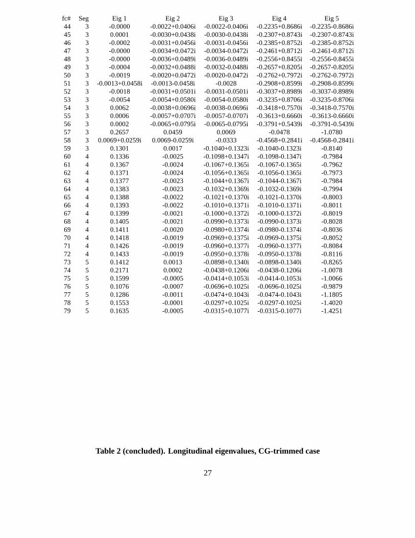
fc# Seg Eig 1 Eig 2 Eig 3 Eig 4 Eig 544 3 -0.0000 -0.0022+0.0406i -0.0022-0.0406i -0.2235+0.8686i -0.2235-0.8686i45 3 0.0001 -0.0030+0.0438i -0.0030-0.0438i -0.2307+0.8743i -0.2307-0.8743i46 3 -0.0002 -0.0031+0.0456i -0.0031-0.0456i -0.2385+0.8752i -0.2385-0.8752i47 3 -0.0000 -0.0034+0.0472i -0.0034-0.0472i -0.2461+0.8712i -0.2461-0.8712i48 3 -0.0000 -0.0036+0.0489i -0.0036-0.0489i -0.2556+0.8455i -0.2556-0.8455i49 3 -0.0004 -0.0032+0.0488i -0.0032-0.0488i -0.2657+0.8205i -0.2657-0.8205i50 3 -0.0019 -0.0020+0.0472i -0.0020-0.0472i -0.2762+0.7972i -0.2762-0.7972i51 3 -0.0013+0.0458i -0.0013-0.0458i -0.0028 -0.2908+0.8599i -0.2908-0.8599i52 3 -0.0018 -0.0031+0.0501i -0.0031-0.0501i -0.3037+0.8989i -0.3037-0.8989i53 3 -0.0054 -0.0054+0.0580i -0.0054-0.0580i -0.3235+0.8706i -0.3235-0.8706i54 3 0.0062 -0.0038+0.0696i -0.0038-0.0696i -0.3418+0.7570i -0.3418-0.7570i55 3 0.0006 -0.0057+0.0707i -0.0057-0.0707i -0.3613+0.6660i -0.3613-0.6660i56 3 0.0002 -0.0065+0.0795i -0.0065-0.0795i -0.3791+0.5439i -0.3791-0.5439i57 3 0.2657 0.0459 0.0069 -0.0478 -1.078058 3 0.0069+0.0259i 0.0069-0.0259i -0.0333 -0.4568+0.2841i -0.4568-0.2841i59 3 0.1301 0.0017 -0.1040+0.1323i -0.1040-0.1323i -0.814060 4 0.1336 -0.0025 -0.1098+0.1347i -0.1098-0.1347i -0.798461 4 0.1367 -0.0024 -0.1067+0.1365i -0.1067-0.1365i -0.796262 4 0.1371 -0.0024 -0.1056+0.1365i -0.1056-0.1365i -0.797363 4 0.1377 -0.0023 -0.1044+0.1367i -0.1044-0.1367i -0.798464 4 0.1383 -0.0023 -0.1032+0.1369i -0.1032-0.1369i -0.799465 4 0.1388 -0.0022 -0.1021+0.1370i -0.1021-0.1370i -0.800366 4 0.1393 -0.0022 -0.1010+0.1371i -0.1010-0.1371i -0.801167 4 0.1399 -0.0021 -0.1000+0.1372i -0.1000-0.1372i -0.801968 4 0.1405 -0.0021 -0.0990+0.1373i -0.0990-0.1373i -0.802869 4 0.1411 -0.0020 -0.0980+0.1374i -0.0980-0.1374i -0.803670 4 0.1418 -0.0019 -0.0969+0.1375i -0.0969-0.1375i -0.805271 4 0.1426 -0.0019 -0.0960+0.1377i -0.0960-0.1377i -0.808472 4 0.1433 -0.0019 -0.0950+0.1378i -0.0950-0.1378i -0.811673 5 0.1412 0.0013 -0.0898+0.1340i -0.0898-0.1340i -0.826574 5 0.2171 0.0002 -0.0438+0.1206i -0.0438-0.1206i -1.007875 5 0.1599 -0.0005 -0.0414+0.1053i -0.0414-0.1053i -1.006676 5 0.1076 -0.0007 -0.0696+0.1025i -0.0696-0.1025i -0.987977 5 0.1286 -0.0011 -0.0474+0.1043i -0.0474-0.1043i -1.180578 5 0.1553 -0.0001 -0.0297+0.1025i -0.0297-0.1025i -1.402079 5 0.1635 -0.0005 -0.0315+0.1077i -0.0315-0.1077i -1.4251

Table 2 (concluded). Longitudinal eigenvalues, CG-trimmed case

27

fc# Seg Eig 1 Eig 2 Eig 3 Eig 41 1 -0.0603 -0.1550+0.9428i -0.1550-0.9428i -1.02772 1 -0.0417 -0.1566+0.9948i -0.1566-0.9948i -1.07333 1 -0.0387 -0.1421+0.8476i -0.1421-0.8476i -1.33154 1 -0.0253 -0.1322+0.9450i -0.1322-0.9450i -1.49145 1 -0.0190 -0.1326+1.0786i -0.1326-1.0786i -1.62366 1 -0.0174 -0.1330+1.0809i -0.1330-1.0809i -1.62397 1 -0.0174 -0.1304+1.0850i -0.1304-1.0850i -1.59768 1 -0.0174 -0.1168+1.1183i -0.1168-1.1183i -1.46689 1 -0.0155 -0.0914+1.1634i -0.0914-1.1634i -1.4064

10 1 -0.0176 -0.0707+1.1226i -0.0707-1.1226i -1.395011 1 -0.0181 -0.0705+1.1227i -0.0705-1.1227i -1.394912 1 -0.0207 -0.0932+1.1618i -0.0932-1.1618i -1.398213 1 -0.0255 -0.1486+1.1968i -0.1486-1.1968i -1.454514 1 -0.0224 -0.1374+1.1734i -0.1374-1.1734i -1.485315 1 -0.0198 -0.1444+1.1613i -0.1444-1.1613i -1.358616 1 -0.0179 -0.1539+1.1344i -0.1539-1.1344i -1.229317 1 -0.0164 -0.1651+1.1085i -0.1651-1.1085i -1.097718 1 -0.0152 -0.1791+1.0910i -0.1791-1.0910i -0.972319 1 -0.0145 -0.1727+1.0888i -0.1727-1.0888i -0.900720 1 -0.0138 -0.1652+1.0837i -0.1652-1.0837i -0.831221 1 -0.0133 -0.1566+1.0722i -0.1566-1.0722i -0.769822 1 -0.0131 -0.1520+1.0652i -0.1520-1.0652i -0.739723 1 -0.0131 -0.1520+1.0652i -0.1520-1.0652i -0.739724 1 -0.0129 -0.1440+1.0521i -0.1440-1.0521i -0.697725 1 -0.0140 -0.1386+0.9588i -0.1386-0.9588i -0.627826 1 -0.0130 -0.1295+0.9199i -0.1295-0.9199i -0.578427 1 -0.0120 -0.1202+0.8749i -0.1202-0.8749i -0.536428 1 -0.0108 -0.1107+0.8228i -0.1107-0.8228i -0.503729 1 -0.0107 -0.1107+0.8228i -0.1107-0.8228i -0.503730 1 -0.0107 -0.1055+0.8124i -0.1055-0.8124i -0.490231 2 -0.0091 -0.1029+0.8615i -0.1029-0.8615i -0.496832 2 -0.0088 -0.0988+0.8546i -0.0988-0.8546i -0.499733 2 -0.0086 -0.0961+0.8485i -0.0961-0.8485i -0.503334 2 -0.0083 -0.0937+0.8424i -0.0937-0.8424i -0.506335 2 -0.0081 -0.0913+0.8362i -0.0913-0.8362i -0.508936 2 -0.0079 -0.0890+0.8299i -0.0890-0.8299i -0.511037 2 -0.0076 -0.0865+0.8240i -0.0865-0.8240i -0.516538 2 -0.0072 -0.0840+0.8191i -0.0840-0.8191i -0.526539 2 -0.0068 -0.0818+0.8139i -0.0818-0.8139i -0.536240 2 -0.0065 -0.0798+0.8088i -0.0798-0.8088i -0.545641 2 -0.0061 -0.0780+0.8035i -0.0780-0.8035i -0.554842 2 -0.0059 -0.0764+0.7967i -0.0764-0.7967i -0.563643 2 -0.0056 -0.0750+0.7894i -0.0750-0.7894i -0.5725

Table 3. Lateral eigenvalues, Stabilator trimmed case

28

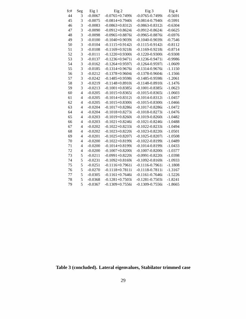
fc# Seg Eig 1 Eig 2 Eig 3 Eig 444 3 -0.0067 -0.0765+0.7499i -0.0765-0.7499i -0.569145 3 -0.0075 -0.0814+0.7940i -0.0814-0.7940i -0.599146 3 -0.0083 -0.0863+0.8312i -0.0863-0.8312i -0.630447 3 -0.0090 -0.0912+0.8624i -0.0912-0.8624i -0.662548 3 -0.0098 -0.0965+0.8876i -0.0965-0.8876i -0.697649 3 -0.0100 -0.1040+0.9039i -0.1040-0.9039i -0.754650 3 -0.0104 -0.1115+0.9142i -0.1115-0.9142i -0.811251 3 -0.0108 -0.1169+0.9218i -0.1169-0.9218i -0.871452 3 -0.0111 -0.1220+0.9300i -0.1220-0.9300i -0.930853 3 -0.0137 -0.1236+0.9471i -0.1236-0.9471i -0.998654 3 -0.0162 -0.1264+0.9597i -0.1264-0.9597i -1.060955 3 -0.0185 -0.1314+0.9676i -0.1314-0.9676i -1.115056 3 -0.0212 -0.1378+0.9604i -0.1378-0.9604i -1.156657 3 -0.0242 -0.1485+0.9598i -0.1485-0.9598i -1.206158 3 -0.0219 -0.1148+0.8910i -0.1148-0.8910i -1.147659 3 -0.0213 -0.1001+0.8385i -0.1001-0.8385i -1.062360 4 -0.0205 -0.1015+0.8365i -0.1015-0.8365i -1.060361 4 -0.0205 -0.1014+0.8312i -0.1014-0.8312i -1.045762 4 -0.0205 -0.1015+0.8300i -0.1015-0.8300i -1.046663 4 -0.0204 -0.1017+0.8286i -0.1017-0.8286i -1.047264 4 -0.0204 -0.1018+0.8273i -0.1018-0.8273i -1.047665 4 -0.0203 -0.1019+0.8260i -0.1019-0.8260i -1.048266 4 -0.0203 -0.1021+0.8246i -0.1021-0.8246i -1.048867 4 -0.0202 -0.1022+0.8233i -0.1022-0.8233i -1.049468 4 -0.0202 -0.1023+0.8220i -0.1023-0.8220i -1.050169 4 -0.0201 -0.1025+0.8207i -0.1025-0.8207i -1.050870 4 -0.0200 -0.1022+0.8199i -0.1022-0.8199i -1.048971 4 -0.0200 -0.1014+0.8199i -0.1014-0.8199i -1.043372 4 -0.0200 -0.1007+0.8200i -0.1007-0.8200i -1.037773 5 -0.0211 -0.0991+0.8220i -0.0991-0.8220i -1.039874 5 -0.0231 -0.1092+0.8169i -0.1092-0.8169i -1.093375 5 -0.0251 -0.1116+0.7961i -0.1116-0.7961i -1.180876 5 -0.0270 -0.1118+0.7811i -0.1118-0.7811i -1.316777 5 -0.0305 -0.1161+0.7646i -0.1161-0.7646i -1.522678 5 -0.0368 -0.1281+0.7503i -0.1281-0.7503i -1.824179 5 -0.0367 -0.1309+0.7556i -0.1309-0.7556i -1.8665

Table 3 (concluded). Lateral eigenvalues, Stabilator trimmed case

29

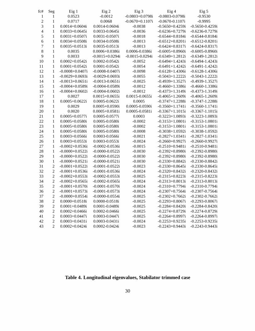
fc# Seg Eig 1 Eig 2 Eig 3 Eig 4 Eig 51 1 0.0523 -0.0012 -0.0803+0.0798i -0.0803-0.0798i -0.95302 1 0.0717 0.0068 -0.0670+0.1107i -0.0670-0.1107i -0.99953 1 0.0014+0.0604i 0.0014-0.0604i -0.0038 -0.5650+0.4259i -0.5650-0.4259i4 1 0.0033+0.0645i 0.0033-0.0645i -0.0036 -0.6236+0.7279i -0.6236-0.7279i5 1 0.0031+0.0507i 0.0031-0.0507i -0.0018 -0.6544+0.8184i -0.6544-0.8184i6 1 0.0034+0.0508i 0.0034-0.0508i -0.0013 -0.6512+0.8201i -0.6512-0.8201i7 1 0.0035+0.0513i 0.0035-0.0513i -0.0013 -0.6424+0.8317i -0.6424-0.8317i8 1 0.0035 0.0006+0.0386i 0.0006-0.0386i -0.6005+0.8960i -0.6005-0.8960i9 1 0.0033 -0.0015+0.0294i -0.0015-0.0294i -0.6349+1.2812i -0.6349-1.2812i

10 1 0.0002+0.0542i 0.0002-0.0542i -0.0052 -0.6494+1.4243i -0.6494-1.4243i11 1 0.0001+0.0542i 0.0001-0.0542i -0.0054 -0.6491+1.4242i -0.6491-1.4242i12 1 -0.0008+0.0407i -0.0008-0.0407i -0.0098 -0.6128+1.4306i -0.6128-1.4306i13 1 -0.0029+0.0693i -0.0029-0.0693i -0.0055 -0.5043+1.2222i -0.5043-1.2222i14 1 -0.0013+0.0651i -0.0013-0.0651i -0.0025 -0.4939+1.3527i -0.4939-1.3527i15 1 -0.0004+0.0589i -0.0004-0.0589i -0.0012 -0.4660+1.3386i -0.4660-1.3386i16 1 -0.0004+0.0602i -0.0004-0.0602i -0.0012 -0.4373+1.3149i -0.4373-1.3149i17 1 0.0027 0.0015+0.0655i 0.0015-0.0655i -0.4065+1.2609i -0.4065-1.2609i18 1 0.0005+0.0622i 0.0005-0.0622i 0.0005 -0.3747+1.2288i -0.3747-1.2288i19 1 0.0029 0.0005+0.0590i 0.0005-0.0590i -0.3560+1.1741i -0.3560-1.1741i20 1 0.0020 0.0005+0.0581i 0.0005-0.0581i -0.3367+1.1015i -0.3367-1.1015i21 1 0.0005+0.0577i 0.0005-0.0577i 0.0003 -0.3223+1.0893i -0.3223-1.0893i22 1 0.0005+0.0580i 0.0005-0.0580i -0.0002 -0.3153+1.0801i -0.3153-1.0801i23 1 0.0005+0.0580i 0.0005-0.0580i -0.0002 -0.3153+1.0801i -0.3153-1.0801i24 1 0.0005+0.0580i 0.0005-0.0580i -0.0008 -0.3038+1.0592i -0.3038-1.0592i25 1 0.0003+0.0566i 0.0003-0.0566i -0.0021 -0.2827+1.0341i -0.2827-1.0341i26 1 0.0003+0.0553i 0.0003-0.0553i -0.0024 -0.2660+0.9927i -0.2660-0.9927i27 1 -0.0002+0.0536i -0.0002-0.0536i -0.0015 -0.2510+0.9481i -0.2510-0.9481i28 1 -0.0000+0.0522i -0.0000-0.0522i -0.0030 -0.2392+0.8980i -0.2392-0.8980i29 1 -0.0000+0.0522i -0.0000-0.0522i -0.0030 -0.2392+0.8980i -0.2392-0.8980i30 1 -0.0000+0.0521i -0.0000-0.0521i -0.0030 -0.2330+0.8842i -0.2330-0.8842i31 2 -0.0001+0.0522i -0.0001-0.0522i -0.0023 -0.2330+0.8645i -0.2330-0.8645i32 2 -0.0001+0.0536i -0.0001-0.0536i -0.0024 -0.2320+0.8432i -0.2320-0.8432i33 2 -0.0002+0.0553i -0.0002-0.0553i -0.0025 -0.2315+0.8223i -0.2315-0.8223i34 2 -0.0002+0.0565i -0.0002-0.0565i -0.0024 -0.2313+0.8013i -0.2313-0.8013i35 2 -0.0001+0.0570i -0.0001-0.0570i -0.0024 -0.2310+0.7794i -0.2310-0.7794i36 2 -0.0001+0.0573i -0.0001-0.0573i -0.0024 -0.2307+0.7564i -0.2307-0.7564i37 2 -0.0000+0.0554i -0.0000-0.0554i -0.0025 -0.2302+0.7662i -0.2302-0.7662i38 2 0.0000+0.0518i 0.0000-0.0518i -0.0025 -0.2293+0.8067i -0.2293-0.8067i39 2 0.0001+0.0489i 0.0001-0.0489i -0.0025 -0.2284+0.8420i -0.2284-0.8420i40 2 0.0002+0.0466i 0.0002-0.0466i -0.0025 -0.2274+0.8729i -0.2274-0.8729i41 2 0.0003+0.0447i 0.0003-0.0447i -0.0025 -0.2264+0.8997i -0.2264-0.8997i42 2 0.0003+0.0431i 0.0003-0.0431i -0.0024 -0.2253+0.9235i -0.2253-0.9235i43 2 0.0002+0.0424i 0.0002-0.0424i -0.0023 -0.2243+0.9443i -0.2243-0.9443i

Table 4. Longitudinal eigenvalues, Stabilator trimmed case

30

fc# Seg Eig 1 Eig 2 Eig 3 Eig 4 Eig544 3 -0.0001 -0.0021+0.0390i -0.0021-0.0390i -0.2245+0.9566i -0.2245-0.9566i45 3 -0.0001 -0.0028+0.0412i -0.0028-0.0412i -0.2320+0.9771i -0.2320-0.9771i46 3 -0.0003 -0.0028+0.0424i -0.0028-0.0424i -0.2400+0.9950i -0.2400-0.9950i47 3 -0.0002 -0.0031+0.0435i -0.0031-0.0435i -0.2480+1.0096i -0.2480-1.0096i48 3 -0.0004 -0.0031+0.0439i -0.0031-0.0439i -0.2581+1.0166i -0.2581-1.0166i49 3 -0.0008 -0.0028+0.0434i -0.0028-0.0434i -0.2686+1.0147i -0.2686-1.0147i50 3 -0.0018+0.0420i -0.0018-0.0420i -0.0023 -0.2793+1.0082i -0.2793-1.0082i51 3 -0.0013+0.0418i -0.0013-0.0418i -0.0031 -0.2938+1.0500i -0.2938-1.0500i52 3 -0.0024 -0.0026+0.0452i -0.0026-0.0452i -0.3071+1.0761i -0.3071-1.0761i53 3 -0.0044+0.0498i -0.0044-0.0498i -0.0065 -0.3280+1.0833i -0.3280-1.0833i54 3 0.0061 -0.0028+0.0548i -0.0028-0.0548i -0.3489+1.0788i -0.3489-1.0788i55 3 -0.0003 -0.0047+0.0531i -0.0047-0.0531i -0.3700+1.0654i -0.3700-1.0654i56 3 -0.0015 -0.0060+0.0552i -0.0060-0.0552i -0.3953+0.9568i -0.3953-0.9568i57 3 -0.0033 -0.0065+0.0552i -0.0065-0.0552i -0.4098+0.5658i -0.4098-0.5658i58 3 0.0001+0.0339i 0.0001-0.0339i -0.0205 -0.4705+0.9422i -0.4705-0.9422i59 3 0.0390 0.0044 -0.0476 -0.4832+0.6328i -0.4832-0.6328i60 4 0.0533 -0.0061 -0.0444 -0.4849+0.6366i -0.4849-0.6366i61 4 0.0539 -0.0059 -0.0451 -0.4785+0.6342i -0.4785-0.6342i62 4 0.0535 -0.0058 -0.0447 -0.4775+0.6355i -0.4775-0.6355i63 4 0.0531 -0.0058 -0.0445 -0.4765+0.6368i -0.4765-0.6368i64 4 0.0528 -0.0058 -0.0442 -0.4754+0.6380i -0.4754-0.6380i65 4 0.0525 -0.0057 -0.0439 -0.4743+0.6392i -0.4743-0.6392i66 4 0.0522 -0.0056 -0.0436 -0.4732+0.6403i -0.4732-0.6403i67 4 0.0517 -0.0056 -0.0433 -0.4721+0.6414i -0.4721-0.6414i68 4 0.0513 -0.0055 -0.0430 -0.4711+0.6424i -0.4711-0.6424i69 4 0.0509 -0.0055 -0.0426 -0.4700+0.6433i -0.4700-0.6433i70 4 0.0508 -0.0054 -0.0427 -0.4692+0.6420i -0.4692-0.6420i71 4 0.0511 -0.0052 -0.0432 -0.4693+0.6386i -0.4693-0.6386i72 4 0.0514 -0.0052 -0.0435 -0.4694+0.6352i -0.4694-0.6352i73 5 0.0367 0.0046 -0.0459 -0.4676+0.6315i -0.4676-0.6315i74 5 0.0838 0.0008 -0.1140 -0.4353+0.1319i -0.4353-0.1319i75 5 0.0472 0.0005 -0.0693 -0.3120 -0.617076 5 0.0340 0.0000 -0.0495 -0.3303 -0.691977 5 0.0286 -0.0023 -0.0581 -0.1644 -0.972878 5 0.0045 -0.0070+0.0579i -0.0070-0.0579i -0.1213 -1.205979 5 0.0006 -0.0083+0.0480i -0.0083-0.0480i -0.1204 -1.2215

Table 4 (continued). Longitudinal eigenvalues, Stabilator trimmed case

31

Form ApprovedOMB No. 0704-0188

Public reporting burden for this collection of information is estimated to average 1 hour per response, including the time for reviewing instructions, searching existing data sources,gathering and maintaining the data needed, and completing and reviewing the collection of information. Send comments regarding this burden estimate or any other aspect of thiscollection of information, including suggestions for reducing this burden, to Washington Headquarters Services, Directorate for Information Operations and Reports, 1215 JeffersonDavis Highway, Suite 1204, Arlington, VA 22202-4302, and to the Office of Management and Budget, Paperwork Reduction Project (0704-0188), Washington, DC 20503.

1

4

9

1

1

1

1

1

N

REPORT DOCUMENTATION PAGE

. AGENCY USE ONLY (Leave blank) 2.

. SPONSORING/MONITORING AGENC

2a. DISTRIBUTION/AVAILABILITY STA

7. SECURITY CLASSIFICATIONOF REPORT

SN 7540-01-280-5500

Lockheed Martin EngineeriLangley Program OfficeHampton, VA 23681-2199

National Aeronautics and SLangley Research CenterHampton, VA 23681-2199

Unclassified–UnlimitedSubject Category 08Availability: NASA CASI (

Unclassified

REPORT DATE 3.

December 1999

Y NAME(S) AND ADDRESS(ES)

TEMENT

18. SECURITY CLASSIFICATIONOF THIS PAGE

ng & Sciences Co.

pace Administration

Distribution: Nons301) 621-0390

Unclassified

REPORT TYPE AND DATES COVERED

Contractor Report
FUNDING NUMBERS . TITLE AND SUBTITLE 5.
. AUTHOR(S)

Cg/Stability Map for the Reference H Cycle 3 Supersonic Transport ConcAlong the High Speed Research Baseline Mission Profile

8

1

1

19. SECURITY CLASSIFIOF ABSTRACT

tandard

Unclassified

eptC NAS1-96014WU 537-07-24-21WBS 4.3.5

6

7. PERFORMING ORGANIZATION NAME(S) AND ADDRESS(ES)

Daniel P. Giesy and David M. Christhilf

. PERFORMING ORGANIZATIONREPORT NUMBER

0. SPONSORING/MONITORINGAGENCY REPORT NUMBER

C

NASA/CR-1999-209527

1. SUPPLEMENTARY NOTES

Langley Technical Monitor: Carey S. Buttrill

2b. DISTRIBUTION CODE

a ref-ft place-total

g usingitudinal

3. ABSTRACT (Maximum 200 words)

A comparison is made between the results of trimming a High Speed Civil Transport (HSCT) concept alongerence mission profile using two trim modes. One mode uses the stabilator. The other mode uses fore and ament of the center of gravity. A comparison is make of the throttle settings (cruise segments) or theacceleration (ascent and descent segments) and of the drag coefficient. The comparative stability of trimminthe two modes is also assessed by comparing the stability margins and the placement of the lateral and longeigenvalues.

4. SUBJECT TERMS 1

1

High Speed Civil Transport; High speed supersonic transport; Longitudinal trVariable center of gravity; Stability

ATION 2

SP2

5. NUMBER OF PAGES

6. PRICE CODE

im; 37

A03
0. LIMITATION
OF ABSTRACT

tandard Form 298 (Rev. 2-89)rescribed by ANSI Std. Z39-1898-102

UL

Cg/Stability Map for the Reference H Cycle 3 Supersonic ...mln/ltrs-pdfs/NASA-99-cr209527.pdf · Cg/Stability Map for the Reference H Cycle 3 Supersonic Transport Concept Along the

Documents