California Wildlife Habitat Relationships

California Wildlife Habitat Relationships Program California Department of Fish and Game

HABITAT SUITABILITY MODELS FOR USE WITH ARC/INFO: VAGRANT SHREW

CWHR Technical Report No. 23 Sacramento, CA June 1995

i

CWHR Technical Report No. 23 June 1995

HABITAT SUITABILITY MODELS FOR USE WITH ARC/INFO: VAGRANT SHREW

by

Irene C. Timossi Ellen L. Woodard Reginald H. Barrett

Department of Environmental Science, Policy, and Management University of California Berkeley, CA 94720

and the Sierra Nevada Ecosystem Project

California Wildlife Habitat Relationships Program California Department of Fish and Game

1807 13th Street, Suite 202 Sacramento, CA 95814

Suggested Citation: Timossi, I. C., E. L. Woodard, and R. H. Barrett. 1995. Habitat suitability models for use

ii

with ARC/INFO: Vagrant shrew. Calif. Dept. of Fish and Game, CWHR Program, Sacramento, CA. CWHR Tech. Report No. 23. 22 pp.

PREFACE

This document is part of the California Wildlife Habitat Relationships (CWHR) System operated and maintained by the California Department of Fish and Game (CDFG) in cooperation with the California Interagency Wildlife Task Group (CIWTG). This information will be useful for environmental assessments and wildlife habitat management.

The structure and style of this series is basically consistent with the "Habitat Suitability Index Models" or "Bluebook" series produced by the USDI, Fish and Wildlife Service (FWS) since 1981. Moreover, models previously published by the FWS form the basis of the current models for all species for which a "Bluebook" is available. As is the case for the "Bluebook" series, this CWHR series is not copyrighted because it is intended that the information should be as freely available as possible. In fact, it is expected that these products will evolve rapidly over the next decade.

This document consists of two major sections. The Habitat Use Information functions as an up-to-date review of our current understanding regarding the basic habitat requirements of the species. This section typically builds on prior publications, including the FWS "Bluebook" series. However, the Habitat Suitability Index (HSI) Model section is quite different from previously published models. All models in this CWHR series are designed as macros (AML computer programs) for use with ARC/INFO geographic information system (GIS) software running on a UNIX platform. As such, they represent a step up in model realism in that spatial issues can be dealt with explicitly. They are "Level II" models in contrast to the "Level I" (matrix) models initially available in the CWHR System. For example, issues such as habitat fragmentation and distance to habitat elements may be dealt with in spatially explicit "Level II" models. Unfortunately, a major constraint remains the unavailability of mapped habitat information most useful in defining a given species' habitat. For example, there are no readily available maps of snag density. Consequently, the models in this series are compromises between the need for more accurate models and the cost of mapping essential habitat characteristics. It is hoped that such constraints will diminish in time.

While "Level II" models incorporate spatial issues, they build on "Level I", nonspatial models maintained in the CWHR System. As the matrix models are field tested, and occasionally modified, these changes will be expressed in the spatial models as well. In other words, the continually evolving "Level I" models are an integral component of the GIS-based, spatial models. To use these "Level II" models one must have (1) UNIX-based ARC/INFO with GRID module, (2) digitized coverages of CWHR habitat types for the area under study and

iii

habitat element maps as required for a given species, (3) the AML presented in this document, and (4) a copy of the CWHR database. Digital copies of AMLs are available from the CWHR Coordinator at the CDFG.

Unlike many HSI models produced for the FWS, this series produces maps of habitat suitability with four classes of habitat quality: (1) None; (2) Low; (3) Medium; and (4) High. These maps must be considered hypotheses in need of testing rather than proven cause and effect relationships, and proper use of the CWHR System requires that field testing be done. The maps are only an initial "best guess" which professional wildlife biologists can use to optimize their field sampling. Reliance on the maps without field testing is risky even if the habitat information is accurate.

The CDFG and CIWTG strongly encourage feedback from users of this model and other CWHR components concerning improvements and other suggestions that may increase the utility and effectiveness of this habitat-based approach to wildlife management planning.

ACKNOWLEDGMENTS

The primary credit for this document must go to the field biologists and naturalists that have published the body of literature on the ecology and natural history of this species. They are listed in the References section. Ecological information of this sort is generally very expensive and time-consuming to obtain. Yet this basic ecological understanding is exactly what is needed most if the goal of accurately predicting changes in distribution and abundance of a particular species is ever to be achieved. The CWHR System is designed to facilitate the use of existing information by practicing wildlife biologists. We hope it will also stimulate funding for basic ecological research. Funding for producing this model was provided by the California Department of Forestry and Fire Protection and the University of California Agricultural Experiment Station.

We thank Barry Garrison, Karyn Sernka, and Sandie Martinez of the California Department of Fish and Game for their assistance in typing, editing, and producing this report.

iv

TABLE OF CONTENTS

PREFACE............................................................................................................................ iii

ACKNOWLEDGMENTS ................................................................................................... iv

HABITAT USE INFORMATION ........................................................................................1General......................................................................................................................1Food .........................................................................................................................1Water ........................................................................................................................1Cover ........................................................................................................................1Reproduction.............................................................................................................2Interspersion and Composition ...................................................................................2Special Considerations ...............................................................................................3

HABITAT SUITABILITY INDEX (HSI) MODEL ...............................................................3Model Applicability....................................................................................................3

Geographic Area............................................................................................3Season...........................................................................................................3Cover Types..................................................................................................3Minimum Habitat Area ...................................................................................3Verification Level...........................................................................................3

Model Description .....................................................................................................4Overview.......................................................................................................4Cover component. .........................................................................................4Distance to Water ..........................................................................................4Species Distribution........................................................................................5Spatial Analysis..............................................................................................5Definitions......................................................................................................5

Application of the Model............................................................................................7Problems with the Approach ......................................................................................8

Cost ..............................................................................................................8Dispersal Distance..........................................................................................8Day to Day Distance. .....................................................................................8

SOURCES OF OTHER MODELS .......................................................................................8

v

REFERENCES .....................................................................................................................9

APPENDIX 1: Vagrant Shrew Macro.................................................................................11

vi

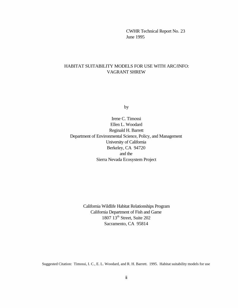
VAGRANT SHREW (Sorex vagrans)

HABITAT USE INFORMATION

General

The vagrant shrew (Sorex vagrans) is found from southern British Columbia south along the coast to northern California. The range extends inland through western Montana and Wyoming, Utah, western Colorado, through eastern Arizona and western New Mexico. In California, the vagrant shrew is common to abundant in the Sierra Nevada and Cascades from the Oregon border to northern Inyo County, and along the coast from the Oregon border to Monterey Bay. Vagrant shrews can be found in California from sea level to 3,750 m (12,000 ft) in a variety of habitats (Burt and Grossenheider 1976; Zeiner et al. 1990).

Food

Vagrant shrews feed mainly on invertebrates such as insects, insect larvae, worms, snails, slugs, and spiders. They also eat fungi, small mammals, roots, young shoots, and probably seeds (Moore 1940; Clothier 1955; Whitaker and Maser 1976; Zeiner et al 1990). Whitaker et al. (1983) reported they ate more flying insects and caterpillars, and fewer terrestrial insects and worms, when grazing pressure was heavy.

They forage under litter on moist surfaces, underground, and in moist accumulations of dead plant material. They often forage in the runways of voles (Microtus spp.) (Whitaker and Maser 1976). They actively forage 24 hours a day.

Water

This species may require water. Clothier (1955) reported that vagrant shrews were not found farther than 180 m (600 ft) from water. In Colorado, Spencer and Pettus (1966) captured shrews an average of 45 m (148 ft) from water. They decided that habitat structure was more important in determining shrew distribution than proximity of water. In a study in California, Ingles (1961) found shrews only in moist habitats.

Cover

Vagrant shrews prefer dense litter or ground cover (Hawes 1977; Zeiner et al. 1990). They do not tunnel in soil like many other shrew species, but create tunnels in leaf litter or ground cover, or use vole runways. Terry (1981) found a positive correlation between vagrant shrew abundance and the depth of the soil organic layer and the humus depth.

1

They are often found in patchy, open areas with wet microhabitats such as damp meadows and stream banks. Along the coast, the vagrant shrew prefers more open, grassy situations than the forest dwelling shrews S. pacificus and S. trowbridgii. In the Sierra Nevada, the vagrant shrew tends to occur at lower elevations and have a weaker relationship to water than the dusky shrew (Sorex monticolus) (Ingles 1961; Spencer and Pettus 1966; Hennings and Hoffmann 1977). In Washington, Terry (1981) found that vagrant shrew abundance was negatively correlated with tall tree cover and percent shrub cover. In Colorado, Spencer and Pettus (1966) found this shrew utilizing wet meadow-bog habitat more than the surrounding forest or clear-cut areas. Ingles (1961) found few vagrant shrews outside of wet meadows in a California study.

S. v. haliocetes is restricted to salt marshes in San Francisco Bay. These shrews prefer a low, dense cover of Salicornia, and occur in low densities (Williams 1986).

Reproduction

The vagrant shrew makes a nest of dry grass, moss, or other materials under logs, roots, or dense vegetation. Brood nests are usually round or oval, 9-14 cm (3.5-5.5 in) in diameter and 5-7 cm (2.0-2.8 in) in height. Construction consists of a loose outer layer and a more compact inner layer. Inner nesting chambers are from 2-3 cm (0.8-1.2 in) in diameter, with one or two exits (Hooven et al. 1975; Zeiner et al. 1990).

After a 20-day gestation period, most young are born from March to May. There may be a second peak of births in August and September. Litter size averages 6 with a range of 2-9 young. There are one to two (rarely three) litters per year. The young are weaned 16-20 days after birth. Females may breed in their first year, and the maximum life span is about 16 months. Most shrews do not live to breed a second year (Clothier 1955; Hooven et al. 1975; Zeiner et al. 1990).

Interspersion and Composition

Breeding home ranges for vagrant shrews averaged 0.33 ha (0.82 ac) and ranged from 0.07-0.53 ha (0.18-1.3 ac) (Hawes 1977). Nonbreeding home ranges averaged 0.10 ha (0.26 ac) and ranged from 0.05-0.20 ha (0.13-0.49 ac) (Hawes 1977). Juvenile home ranges were similar to those of nonbreeding adults.

Adult vagrant shrews are solitary except for the breeding season, when there is extensive home range overlap. Adults begin defending their home ranges from other adults (not juveniles) in late summer and continue to do so until the next mating season (Zeiner et al. 1990).

2

Special Considerations

S. v. halicoetes is restricted to salt marshes in the San Francisco Bay area. Most suitable habitat has been lost to development. The vagrant shrew occurs in low densities and may require protection. S.v. halicoetes is a California Species of Special concern (Williams 1986).

HABITAT SUITABILITY INDEX (HSI) MODEL

Model Applicability

Geographic Area

The California Wildlife Habitat Relationships (CWHR) System (Airola 1988; Mayer and Laudenslayer; 1988, Zeiner et al. 1990) contains habitat ratings for each habitat type predicted to be occupied by vagrant shrew in California.

Season

This model is designed to predict the suitability of habitat for vagrant shrews throughout the year. The model works best at predicting habitat suitability for breeding habitat..

Cover Types

This model can be used anywhere in California for which an ARC/INFO map of CWHR habitat types exists. The CWHR System contains suitability ratings for reproduction, cover, and feeding for all habitats vagrant shrews are predicted to occupy. These ratings can be used in conjunction with the ARC/INFO habitat map to model wildlife habitat suitability.

Minimum Habitat Area

Minimum habitat area is defined as the minimum amount of contiguous habitat required before a species will occupy an area. Specific information on minimum areas required for vagrant shrew was not found in the literature. This model assumes two home ranges is the minimum area required to support a vagrant shrew population during the breeding season.

Verification Level

The spatial model presented here has not been verified in the field. The CWHR suitability

3

values used are based on a combination of literature searches and expert opinion. We strongly encourage field testing of both the CWHR database and this spatial model.

Model Description

Overview

This model uses CWHR habitat type as the main factor determining suitability of an area for this species.

A CWHR habitat type map must be constructed in ARC/INFO GRID format as a basis for the model. The GRID module of ARC/INFO was used because of its superior functionality for spatial modeling. Only crude spatial modeling is possible in the vector portion of the ARC/INFO program, and much of the modeling done here would have been impossible without the abilities of the GRID module. In addition to more sophisticated modeling, the GRID module’s execution speed is very rapid, allowing a complex model to run in less than 30 minutes.

The following sections document the logic and assumptions used to interpret habitat suitability.

Cover Component

A CWHR habitat map must be constructed. The mapped data (coverage) must be in ARC/INFO GRID format. A grid is a GIS coverage composed of a matrix of information. When the grid coverage is created, the size of the grid cell should be determined based on the resolution of the habitat data and the home range size of the species with the smallest home range in the study. You must be able to map the home range of the smallest species with reasonable accuracy. However, if the cell size becomes too small, data processing time can increase considerably. We recommend a grid cell size of 30 m (98 ft). Each grid cell can be assigned attributes. The initial map must have an attribute identifying the CWHR habitat type of each grid cell. A CWHR suitability value is assigned to each grid cell in the coverage based on its habitat type. Each CWHR habitat is rated as high, medium, low or of no value for each of three life requisites: reproduction; feeding; and cover. The geometric mean value of the three suitability values was used to determine the base value of each cell for this analysis.

Distance to Wate.

No water requirement was found for this species.

Species Distribution

4

The study area must be manually compared to the range maps in the CWHR Species Notes (Zeiner et al. 1990) to ensure that it is within the species' range. All grid cells outside the species' range have a suitability of zero.

Spatial Analysis

Ideally, a spatial model of distribution should operate on coverages containing habitat element information of primary importance to a species. For example, in the case of woodpeckers, the size and density of snags as well as the vegetation type would be of great importance. For many small rodents, the amount and size of dead and down woody material would be important. Unfortunately, the large cost involved in collecting microhabitat (habitat element) information and keeping it current makes it likely that geographic information system (GIS) coverages showing such information will be unavailable for extensive areas into the foreseeable future.

The model described here makes use of readily available information such as CWHR habitat type, elevation, slope, aspect, roads, rivers, streams and lakes. The goal of the model is to eliminate areas that are unlikely to be utilized by the species and lessen the value of marginally suitable areas. It does not attempt to address all the microhabitat issues discussed above, nor does it account for other environmental factors such as toxins, competitors or predators. If and when such information becomes available, this model could be modified to make use of it.

In conclusion, field surveys will likely discover that the species is not as widespread or abundant as predictions by this model suggest. The model predicts potentially available habitat. There are a variety of reasons why the habitat may not be utilized.

Definitions

Home Range: the area regularly used for all life activities by an individual during the season(s) for which this model is applicable.

Dispersal Distance: the distance an individual will disperse to establish a new home range. In this model it is used to determine if Potential Colony Habitat will be utilized.

Day to Day Distance: the distance an individual is willing to travel on a daily or semi-daily basis to utilize a distant resource (Potential Day to Day Habitat). The distance used in the model is the home range radius. This is determined by calculating the radius of a circle with an area of one home range.

5

Core Habitat: a contiguous area of habitat of medium or high quality that has an area greater than two home ranges. This habitat is in continuous use by the species. The species is successful enough in this habitat to produce offspring that may disperse from this area to the Colony Habitat or Other Habitat.

Potential Colony Habitat: a contiguous area of habitat of medium or high quality that has an area between one and two home ranges. It is not necessarily used continuously by the species. The distance from a core area will affect how often Potential Colony Habitat is utilized.

Colony Habitat: Potential Colony Habitat that is within the dispersal distance of the species. These areas receive their full original value unless they are further than three home range radii from a core area. These distant areas receive a value of low since there is a low probability that they will be utilized regularly.

Potential Day to Day Habitat: an area of high or medium quality habitat less than one home range, or habitat of low quality of any size. This piece of habitat alone is too small or of inadequate quality to be Core Habitat.

Day to Day Habitat: Potential Day to Day Habitat that is close enough to Core or Colony Habitat can be utilized by individuals moving out from those areas on a day to day basis. The grid cell must be within Day to Day Distance of Core or Colony Habitat.

Other Habitat: contiguous areas of low value habitat larger than two home ranges in size, including small areas of high and medium quality habitat that may be imbedded in them, are included as usable habitat by the species. Such areas may act as “sinks” because long-term reproduction may not match mortality.

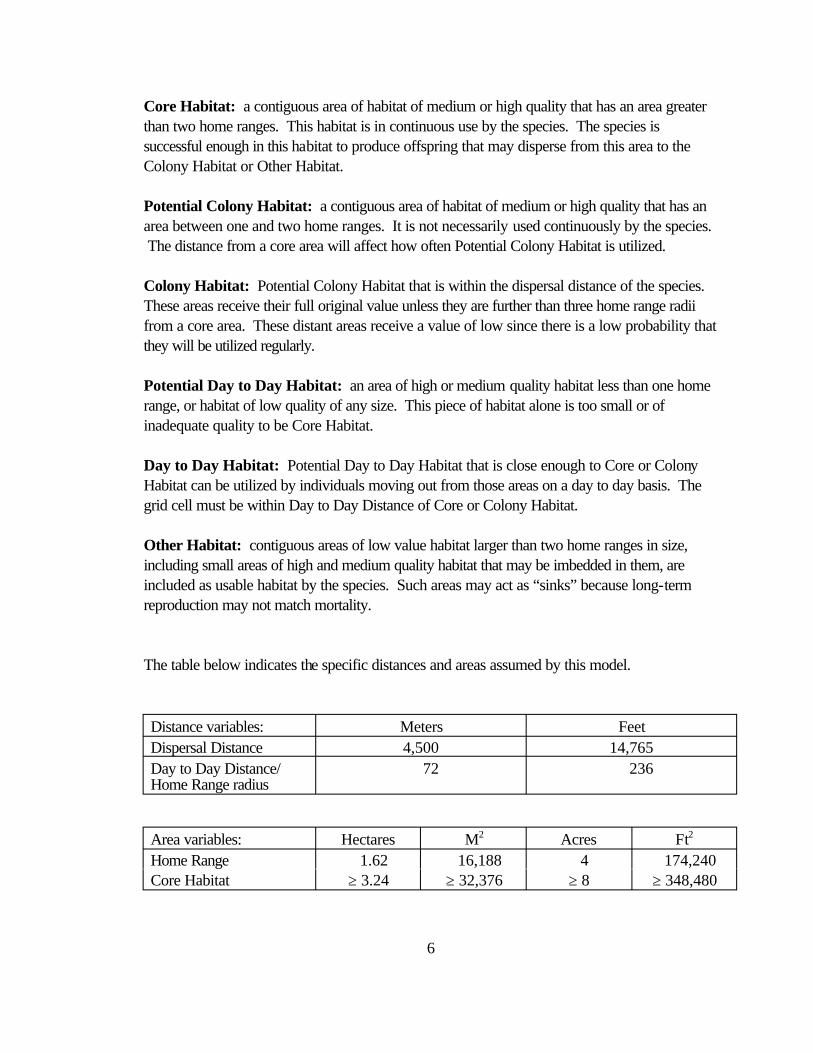
The table below indicates the specific distances and areas assumed by this model.

Distance variables: Meters Feet Dispersal Distance 4,500 14,765 Day to Day Distance/ 72 236 Home Range radius

Area variables: Hectares M2 Acres Ft2

Home Range 1.62 16,188 4 174,240 Core Habitat ‡ 3.24 ‡ 32,376 ‡ 8 ‡ 348,480

6

Application of the Model

A copy of the ARC/INFO AML can be found in Appendix 1. The steps carried out by the macro are as follows:

1. Determine Core Habitat: this is done by first converting all medium quality habitat to high quality habitat and removing all low value habitat. Then contiguous areas of habitat are grouped into regions. The area of each of the regions is determined. Those large enough (‡ two home ranges) are maintained in the Core Habitat coverage. If no Core Habitat is identified then the model will indicate no suitable habitat in the study area.

2. Identify Potential Colony Habitat: using the coverage from Step 1, determine which regions are one to two home ranges in size. These are Potential Colonies.

3. Identify Potential Day Use Habitat: using the coverage derived in Step 1, determine which areas qualify as Potential Day to Day Habitat.

4. Calculate the Cost Grid: since it is presumed to be more difficult for animals to travel through unsuitable habitat than suitable habitat, we use a cost grid to limit travel based on habitat suitability. The cost to travel is one for high or medium quality habitat. This means that to travel 1 m through this habitat costs 1 m of Dispersal Distance. The cost to travel through low quality habitat is two and unsuitable habitat costs four. This means that to travel 1 m through unsuitable habitat costs the species 4 m of Dispersal Distance.

5. Calculate the Cost Distance Grid: a cost distance grid containing the minimum cost to travel from each grid cell to the closest Core Habitat is then calculated using the Cost Grid (Step 4) and the Core Habitat (Step 1).

6. Identify Colony Habitat: based on the Cost Distance Grid (Step 5), only Potential Colony Habitat within the Dispersal Distance of the species to Core Habitat is retained. Colonies are close enough if any cell in the Colony is within the Dispersal Distance from Core Habitat. The suitability of any Colony located further than three home range radii from a Core Habitat is changed to low since it is unlikely it will be utilized regularly.

7. Create the Core + Colony Grid: combine the Core Habitat (Step 1) and the Colony Habitat (Step 6) and calculate the cost to travel from any cell to Core or Colony Habitat. This is used to determine which Potential Day to Day Habitat could be utilized.

7

8. Identify Day to Day Habitat: grid cells of Day to Day Habitat are only accessible to the species if they are within Day to Day Distance from the edge of the nearest Core or Colony Habitat. Add these areas to the Core + Colony Grid (Step 7).

9. Add Other Habitat: large areas (‡ two home ranges in size) of low value habitat, possibly with small areas of high and medium habitat imbedded in them may be utilized, although marginally. Add these areas back into the Core + Colony + Day to Day Grid (Step 8), if any exist, to create the grid showing areas that will potentially be utilized by the species. Each grid cell contains a one if it is utilized and a zero if it is not.

10. Restore Values: all areas that have been retained as having positive habitat value receive their original geometric mean value from the original geometric value grid (see Cover component section) with the exception of distant colonies. Distant colonies (colonies more than three home range radii distant) have their value reduced to low because of the low likelihood of utilization.

Problems with the Approach

Cost

The cost to travel across low suitability and unsuitable habitat is not known. It is likely that it is quite different for different species. This model incorporates a reasonable guess for the cost of movement. A small bird will cross unsuitable habitat much more easily than a small mammal. To some extent differences in agility between species is accounted for by different estimates of dispersal distances.

Dispersal Distance

The distance animals are willing to disperse from their nest or den site is not well understood. We have used distances from studies of the species or similar species when possible, otherwise first approximations are used. More research is urgently needed on wildlife dispersal.

Day to Day Distance

The distance animals are willing to travel on a day to day basis to use distant resources has not been quantified for most species. This issue is less of a concern than dispersal distance since the possible distances are much more limited, especially with small mammals, reptiles, and amphibians. Home range size is assumed to be correlated with this coefficient.

8

SOURCES OF OTHER MODELS

No other habitat models were found for the vagrant shrew.

REFERENCES

Airola, D.A. 1988. Guide to the California Wildlife Habitat Relationships System. Calif. Dept. of Fish and Game, Sacramento, California. 74 pp.

Clothier, R.R. 1955. Contribution to the life history of Sorex vagrans in Montana. J. Mamm. 36(2):214-221.

Hall, E.R. 1981. The Mammals of North America. 2nd ed. 2 vols. John Wiley and Sons, New York. 1271 pp.

Hawes, M.L. 1977, Home range, territoriality, and ecological separation in sympatric shrews, Sorex vagrans and Sorex obscurus. J. Mamm. 58(3): 354-367.

Hooven, E.F., R.F. Hoyer, and R.M. Storm. 1975. Notes on the vagrant shrew, Sorex vagrans, in the Willamette Valley of western Oregon. Northwest Sci. 49(3):163-173.

Ingles, L.G. 1961. Home range and habits of the wandering shrew. J. Mamm. 42(4): 455­462.

Ingles, L. 1965. Mammals of the Pacific States. Stanford Univ. Press, Stanford, California. 506 pp.

Maser, C., B.R. Mate, J.F. Franklin, and C.T. Dyrness. 1981. Natural history of Oregon coast mammals. USDA, For. Serv., Pac. NW For. and Range Expt. Stat., Gen. Tech. Rep. PNW-133.

Mayer, K.E., and W.F. Laudenslayer, Jr., eds. 1988. A guide to wildlife habitats of California. Calif. Dept. of Fish and Game, Sacramento, California. 166 pp.

Moore, A.W. 1940. Wild animal damage to seed and seedlings on cut-over Douglas-fir lands of Oregon and Washington. USDA Tech. Bull. No. 706. 27 pp.

Rudd, R.L. 1955. Age, sex, and weight comparisons in three species of shrews. J. Mamm. 36(3):323-339.

9

Spencer, A.W., and D. Pettus. 1966. Habitat preferences of five sympatric species of long-tailed shrews. Ecology 47(4):677-683. Terry, C.J. 1981. Habitat differentiation among three species of Sorex and Neurotrichus gibbsi in Washington. Amer. Midl. Natur. 106(1):119-125.

Whitaker, J.O. Jr., S.P. Crow, and C. Maser. 1983. Food of vagrant shrews (Sorex vagrans) from Grant County, Oregon, as related to livestock grazing pressures. Northwest Sci. 57(2):107-111.

Whitaker, J.O. Jr., C. Maser. 1976. Food habits of five western Oregon shrews. Northwest Sci. 50(2):102-107.

Williams, D.F. 1986. Mammalian species of special concern in California. Calif. Dept. Fish and Game, Sacramento, California. Wildl. Mgmt. Div. Admin. Rep. 86-1. 112 pp.

Zeiner, D.C., W.F. Laudenslayer, Jr., K.E. Mayer, and M. White, eds. 1990. California's Wildlife. Vol. 3. Mammals. Calif. Dept. Fish and Game, Sacramento, California. 407 pp.

10

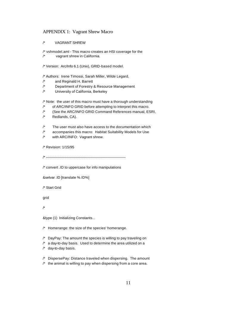
APPENDIX 1: Vagrant Shrew Macro

/* VAGRANT SHREW

/* vshmodel.aml - This macro creates an HSI coverage for the /* vagrant shrew in California.

/* Version: Arc/Info 6.1 (Unix), GRID-based model.

/* Authors: Irene Timossi, Sarah Miller, Wilde Legard, /* and Reginald H. Barrett /* Department of Forestry & Resource Management /* University of California, Berkeley

/* Note: the user of this macro must have a thorough understanding /* of ARC/INFO GRID before attempting to interpret this macro. /* (See the ARC/INFO GRID Command References manual, ESRI, /* Redlands, CA).

/* The user must also have access to the documentation which /* accompanies this macro: Habitat Suitability Models for Use /* with ARC/INFO: Vagrant shrew.

/* Revision: 1/15/95

/* ------------------------------------------------------------------­

/* convert .ID to uppercase for info manipulations

&setvar .ID [translate %.ID%]

/* Start Grid

grid

/*

&type (1) Initializing Constants...

/* Homerange: the size of the species' homerange.

/* DayPay: The amount the species is willing to pay traveling on /* a day-to-day basis. Used to determine the area utilized on a /* day-to-day basis.

/* DispersePay: Distance traveled when dispersing. The amount /* the animal is willing to pay when dispersing from a core area.

11

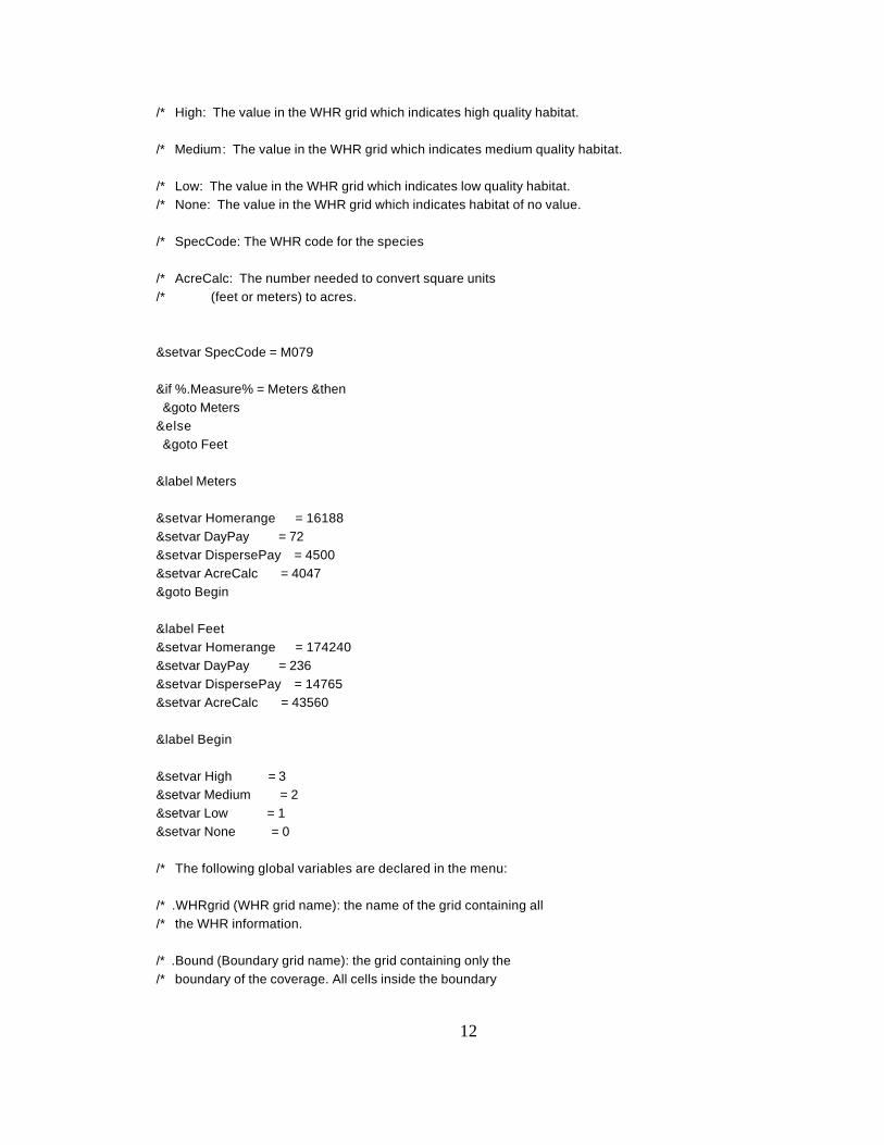
/* High: The value in the WHR grid which indicates high quality habitat.

/* Medium: The value in the WHR grid which indicates medium quality habitat.

/* Low: The value in the WHR grid which indicates low quality habitat. /* None: The value in the WHR grid which indicates habitat of no value.

/* SpecCode: The WHR code for the species

/* AcreCalc: The number needed to convert square units /* (feet or meters) to acres.

&setvar SpecCode = M079

&if %.Measure% = Meters &then &goto Meters &else &goto Feet

&label Meters

&setvar Homerange = 16188 &setvar DayPay = 72 &setvar DispersePay = 4500 &setvar AcreCalc = 4047 &goto Begin

&label Feet &setvar Homerange = 174240 &setvar DayPay = 236 &setvar DispersePay = 14765 &setvar AcreCalc = 43560

&label Begin

&setvar High = 3 &setvar Medium = 2 &setvar Low = 1 &setvar None = 0

/* The following global variables are declared in the menu:

/* .WHRgrid (WHR grid name): the name of the grid containing all /* the WHR information.

/* .Bound (Boundary grid name): the grid containing only the /* boundary of the coverage. All cells inside the boundary

12

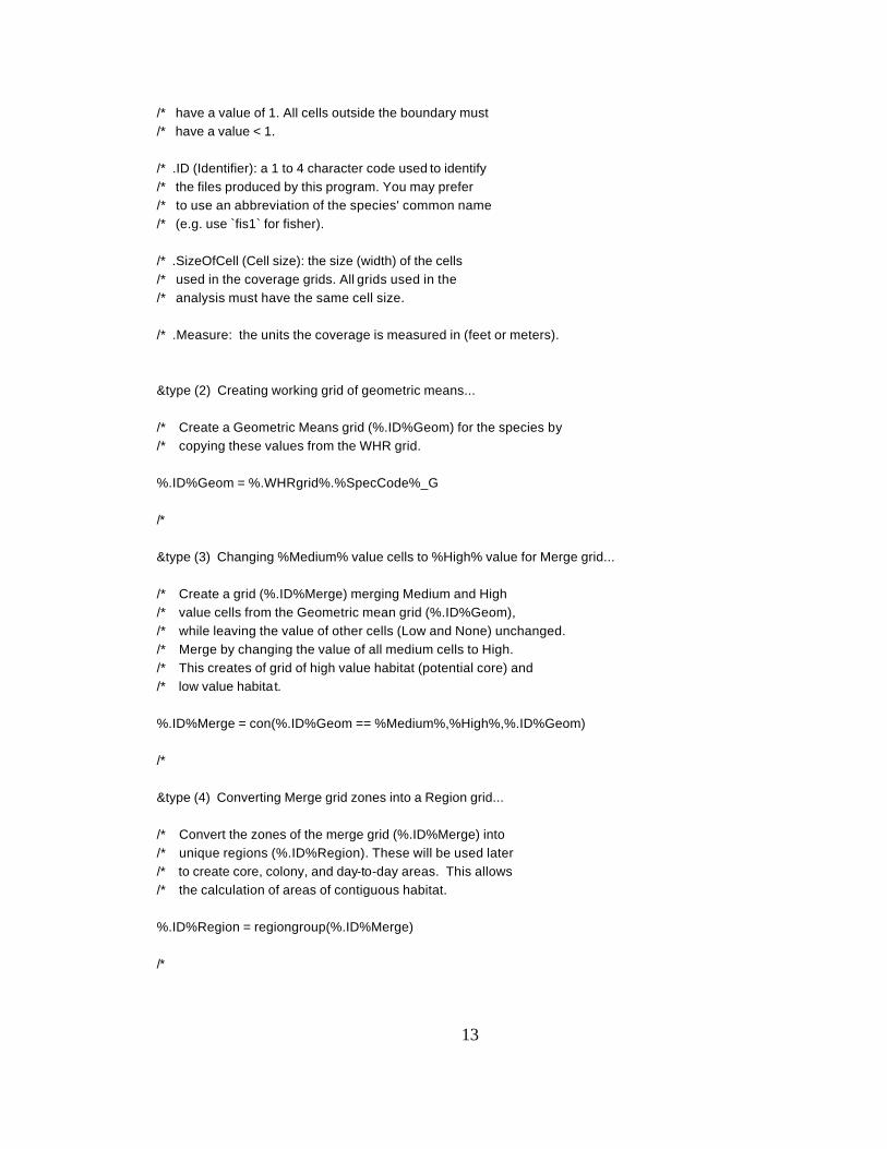
/* have a value of 1. All cells outside the boundary must /* have a value < 1.

/* .ID (Identifier): a 1 to 4 character code used to identify /* the files produced by this program. You may prefer /* to use an abbreviation of the species' common name /* (e.g. use `fis1` for fisher).

/* .SizeOfCell (Cell size): the size (width) of the cells /* used in the coverage grids. All grids used in the /* analysis must have the same cell size.

/* .Measure: the units the coverage is measured in (feet or meters).

&type (2) Creating working grid of geometric means...

/* Create a Geometric Means grid (%.ID%Geom) for the species by /* copying these values from the WHR grid.

%.ID%Geom = %.WHRgrid%.%SpecCode%_G

/*

&type (3) Changing %Medium% value cells to %High% value for Merge grid...

/* Create a grid (%.ID%Merge) merging Medium and High /* value cells from the Geometric mean grid (%.ID%Geom), /* while leaving the value of other cells (Low and None) unchanged. /* Merge by changing the value of all medium cells to High. /* This creates of grid of high value habitat (potential core) and /* low value habitat.

%.ID%Merge = con(%.ID%Geom == %Medium%,%High%,%.ID%Geom)

/*

&type (4) Converting Merge grid zones into a Region grid...

/* Convert the zones of the merge grid (%.ID%Merge) into /* unique regions (%.ID%Region). These will be used later /* to create core, colony, and day-to-day areas. This allows /* the calculation of areas of contiguous habitat.

%.ID%Region = regiongroup(%.ID%Merge)

/*

13

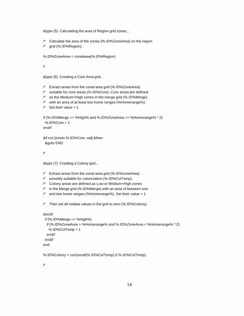
&type (5) Calculating the area of Region grid zones...

/* Calculate the area of the zones (%.ID%ZoneArea) on the region /* grid (%.ID%Region).

%.ID%ZoneArea = zonalarea(%.ID%Region)

/*

&type (6) Creating a Core Area grid...

/* Extract areas from the zonal area grid (%.ID%ZoneArea) /* suitable for core areas (%.ID%Core). Core areas are defined /* as the Medium+High zones in the merge grid (%.ID%Merge) /* with an area of at least two home ranges (%Homerange%). /* Set their value = 1.

if (%.ID%Merge == %High% and %.ID%ZoneArea >= %Homerange% * 2) %.ID%Core = 1 endif

&if not [exists %.ID%Core -vat] &then &goto END

/*

&type (7) Creating a Colony grid...

/* Extract areas from the zonal area grid (%.ID%zoneArea) /* possibly suitable for colonization (%.ID%ColTemp). /* Colony areas are defined as Low or Medium+High zones /* in the Merge grid (%.ID%Merge) with an area of between one /* and two home ranges (%Homerange%). Set their value = 1.

/* Then set all nodata values in the grid to zero (%.ID%Colony).

docell if (%.ID%Merge == %High%) if (%.ID%ZoneArea > %Homerange% and %.ID%ZoneArea < %Homerange% * 2)

%.ID%ColTemp = 1 endif

endif end

%.ID%Colony = con(isnull(%.ID%ColTemp),0,%.ID%ColTemp)

/*

14

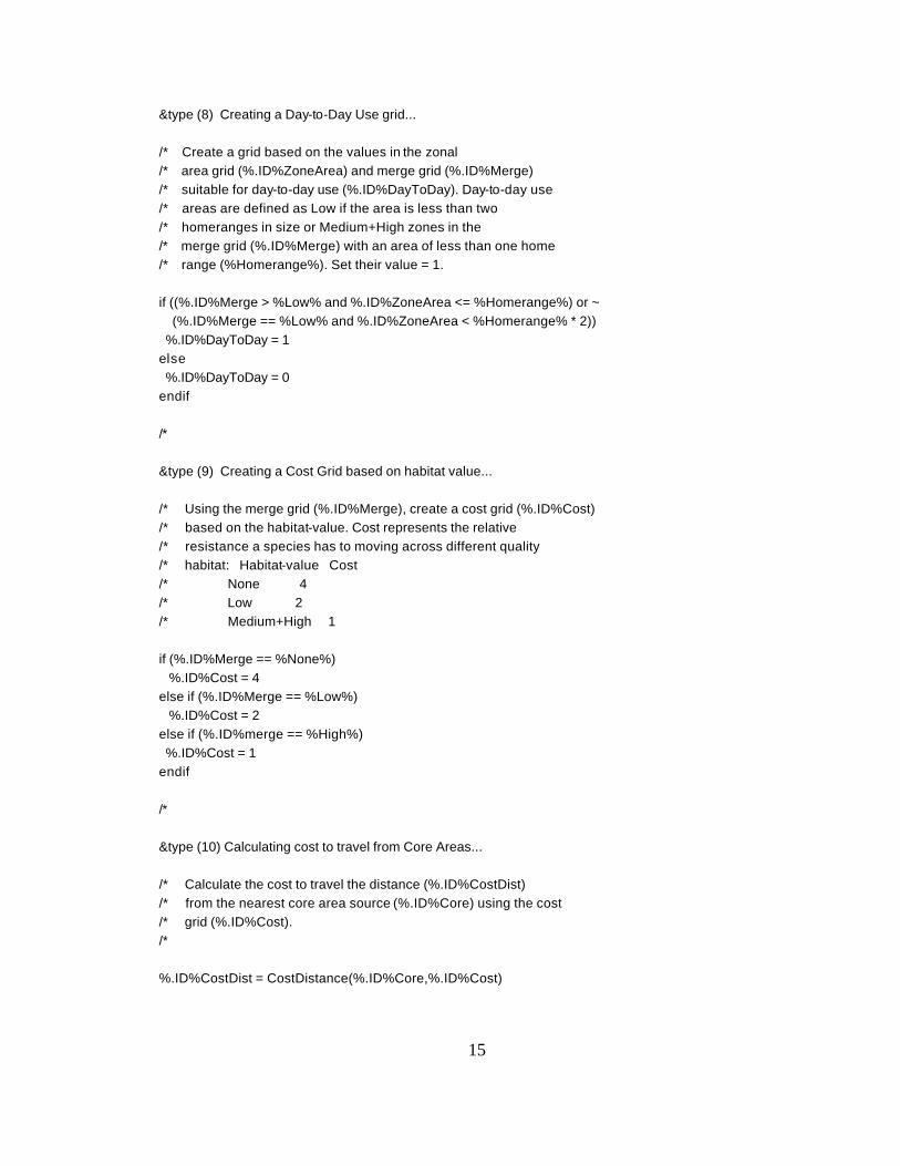
&type (8) Creating a Day-to-Day Use grid...

/* Create a grid based on the values in the zonal /* area grid (%.ID%ZoneArea) and merge grid (%.ID%Merge) /* suitable for day-to-day use (%.ID%DayToDay). Day-to-day use /* areas are defined as Low if the area is less than two /* homeranges in size or Medium+High zones in the /* merge grid (%.ID%Merge) with an area of less than one home /* range (%Homerange%). Set their value = 1.

if ((%.ID%Merge > %Low% and %.ID%ZoneArea <= %Homerange%) or ~ (%.ID%Merge == %Low% and %.ID%ZoneArea < %Homerange% * 2))

%.ID%DayToDay = 1 else %.ID%DayToDay = 0 endif

/*

&type (9) Creating a Cost Grid based on habitat value...

/* Using the merge grid (%.ID%Merge), create a cost grid (%.ID%Cost) /* based on the habitat-value. Cost represents the relative /* resistance a species has to moving across different quality /* habitat: Habitat-value Cost /* None 4 /* Low 2 /* Medium+High 1

if (%.ID%Merge == %None%) %.ID%Cost = 4

else if (%.ID%Merge == %Low%) %.ID%Cost = 2

else if (%.ID%merge == %High%) %.ID%Cost = 1 endif

/*

&type (10) Calculating cost to travel from Core Areas...

/* Calculate the cost to travel the distance (%.ID%CostDist)/* from the nearest core area source (%.ID%Core) using the cost/* grid (%.ID%Cost). /*

%.ID%CostDist = CostDistance(%.ID%Core,%.ID%Cost)

15

/*

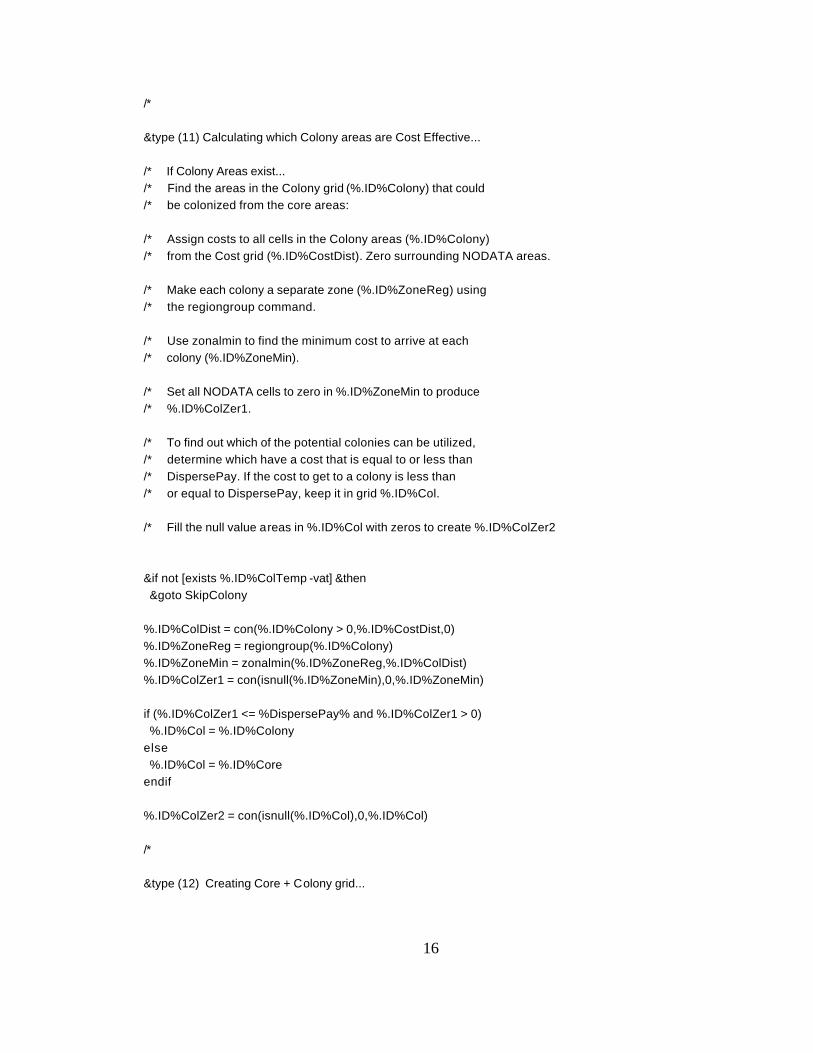
&type (11) Calculating which Colony areas are Cost Effective...

/* If Colony Areas exist.../* Find the areas in the Colony grid (%.ID%Colony) that could

/* be colonized from the core areas:

/* Assign costs to all cells in the Colony areas (%.ID%Colony) /* from the Cost grid (%.ID%CostDist). Zero surrounding NODATA areas.

/* Make each colony a separate zone (%.ID%ZoneReg) using

/* the regiongroup command.

/* Use zonalmin to find the minimum cost to arrive at each

/* colony (%.ID%ZoneMin).

/* Set all NODATA cells to zero in %.ID%ZoneMin to produce

/* %.ID%ColZer1.

/* To find out which of the potential colonies can be utilized,/* determine which have a cost that is equal to or less than

/* DispersePay. If the cost to get to a colony is less than

/* or equal to DispersePay, keep it in grid %.ID%Col.

/* Fill the null value areas in %.ID%Col with zeros to create %.ID%ColZer2

&if not [exists %.ID%ColTemp -vat] &then &goto SkipColony

%.ID%ColDist = con(%.ID%Colony > 0,%.ID%CostDist,0)%.ID%ZoneReg = regiongroup(%.ID%Colony)%.ID%ZoneMin = zonalmin(%.ID%ZoneReg,%.ID%ColDist)%.ID%ColZer1 = con(isnull(%.ID%ZoneMin),0,%.ID%ZoneMin)

if (%.ID%ColZer1 <= %DispersePay% and %.ID%ColZer1 > 0) %.ID%Col = %.ID%Colony else %.ID%Col = %.ID%Core endif

%.ID%ColZer2 = con(isnull(%.ID%Col),0,%.ID%Col)

/*

&type (12) Creating Core + Colony grid...

16

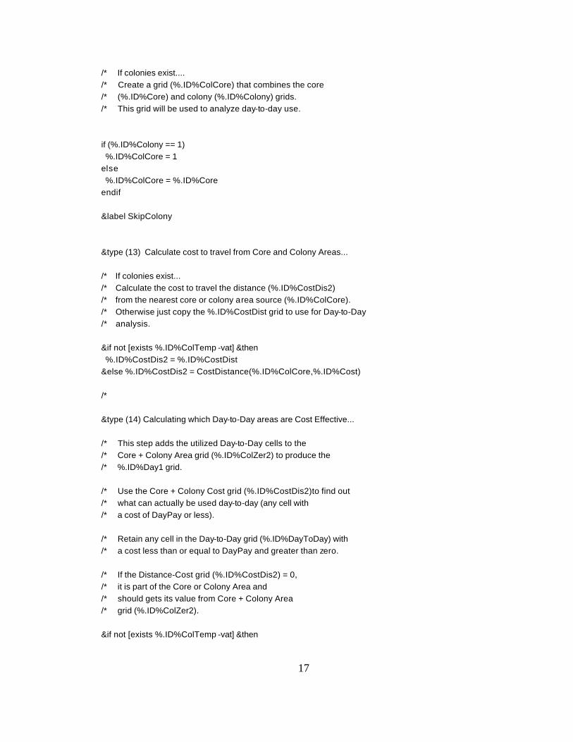
/* If colonies exist..../* Create a grid (%.ID%ColCore) that combines the core /* (%.ID%Core) and colony (%.ID%Colony) grids./* This grid will be used to analyze day-to-day use.

if (%.ID%Colony == 1) %.ID%ColCore = 1 else %.ID%ColCore = %.ID%Core endif

&label SkipColony

&type (13) Calculate cost to travel from Core and Colony Areas...

/* If colonies exist.../* Calculate the cost to travel the distance (%.ID%CostDis2)/* from the nearest core or colony area source (%.ID%ColCore)./* Otherwise just copy the %.ID%CostDist grid to use for Day-to-Day

/* analysis.

&if not [exists %.ID%ColTemp -vat] &then %.ID%CostDis2 = %.ID%CostDist &else %.ID%CostDis2 = CostDistance(%.ID%ColCore,%.ID%Cost)

/*

&type (14) Calculating which Day-to-Day areas are Cost Effective...

/* This step adds the utilized Day-to-Day cells to the /* Core + Colony Area grid (%.ID%ColZer2) to produce the /* %.ID%Day1 grid.

/* Use the Core + Colony Cost grid (%.ID%CostDis2)to find out /* what can actually be used day-to-day (any cell with /* a cost of DayPay or less).

/* Retain any cell in the Day-to-Day grid (%.ID%DayToDay) with /* a cost less than or equal to DayPay and greater than zero.

/* If the Distance-Cost grid (%.ID%CostDis2) = 0, /* it is part of the Core or Colony Area and /* should gets its value from Core + Colony Area /* grid (%.ID%ColZer2).

&if not [exists %.ID%ColTemp -vat] &then

17

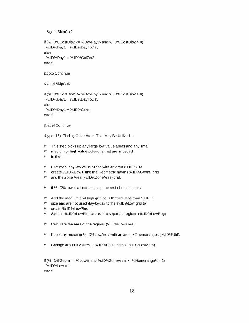
&goto SkipCol2

if (%.ID%CostDis2 <= %DayPay% and %.ID%CostDis2 > 0) %.ID%Day1 = %.ID%DayToDay else %.ID%Day1 = %.ID%ColZer2 endif

&goto Continue

&label SkipCol2

if (%.ID%CostDis2 <= %DayPay% and %.ID%CostDis2 > 0) %.ID%Day1 = %.ID%DayToDay else %.ID%Day1 = %.ID%Core endif

&label Continue

&type (15) Finding Other Areas That May Be Utilized....

/* This step picks up any large low value areas and any small /* medium or high value polygons that are imbeded /* in them.

/* First mark any low value areas with an area > HR * 2 to /* create %.ID%Low using the Geometric mean (%.ID%Geom) grid /* and the Zone Area (%.ID%ZoneArea) grid.

/* if %.ID%Low is all nodata, skip the rest of these steps.

/* Add the medium and high grid cells that are less than 1 HR in /* size and are not used day-to-day to the %.ID%Low grid to /* create %.ID%LowPlus /* Split all %.ID%LowPlus areas into separate regions (%.ID%LowReg)

/* Calculate the area of the regions (%.ID%LowArea).

/* Keep any region in %.ID%LowArea with an area > 2 homeranges (%.ID%Util).

/* Change any null values in %.ID%Util to zeros (%.ID%LowZero).

if (%.ID%Geom == %Low% and %.ID%ZoneArea >= %Homerange% * 2) %.ID%Low = 1 endif

18

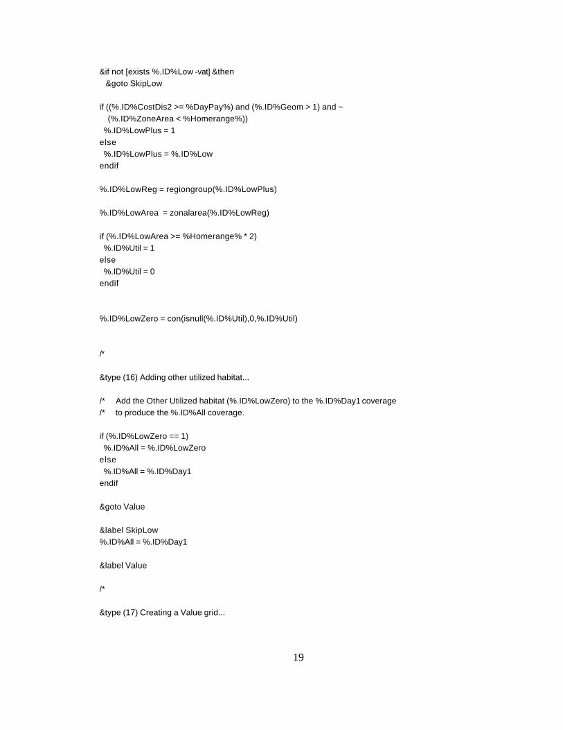
&if not [exists %.ID%Low -vat] &then &goto SkipLow

if ((%.ID%CostDis2 >= %DayPay%) and (%.ID%Geom > 1) and ~ (%.ID%ZoneArea < %Homerange%))

%.ID%LowPlus = 1 else %.ID%LowPlus = %.ID%Low endif

%.ID%LowReg = regiongroup(%.ID%LowPlus)

%.ID%LowArea = zonalarea(%.ID%LowReg)

if (%.ID%LowArea >= %Homerange% * 2) %.ID%Util = 1 else %.ID%Util = 0

endif

%.ID%LowZero = con(isnull(%.ID%Util),0,%.ID%Util)

/*

&type (16) Adding other utilized habitat...

/* Add the Other Utilized habitat (%.ID%LowZero) to the %.ID%Day1 coverage /* to produce the %.ID%All coverage.

if (%.ID%LowZero == 1) %.ID%All = %.ID%LowZero else %.ID%All = %.ID%Day1 endif

&goto Value

&label SkipLow %.ID%All = %.ID%Day1

&label Value

/*

&type (17) Creating a Value grid...

19

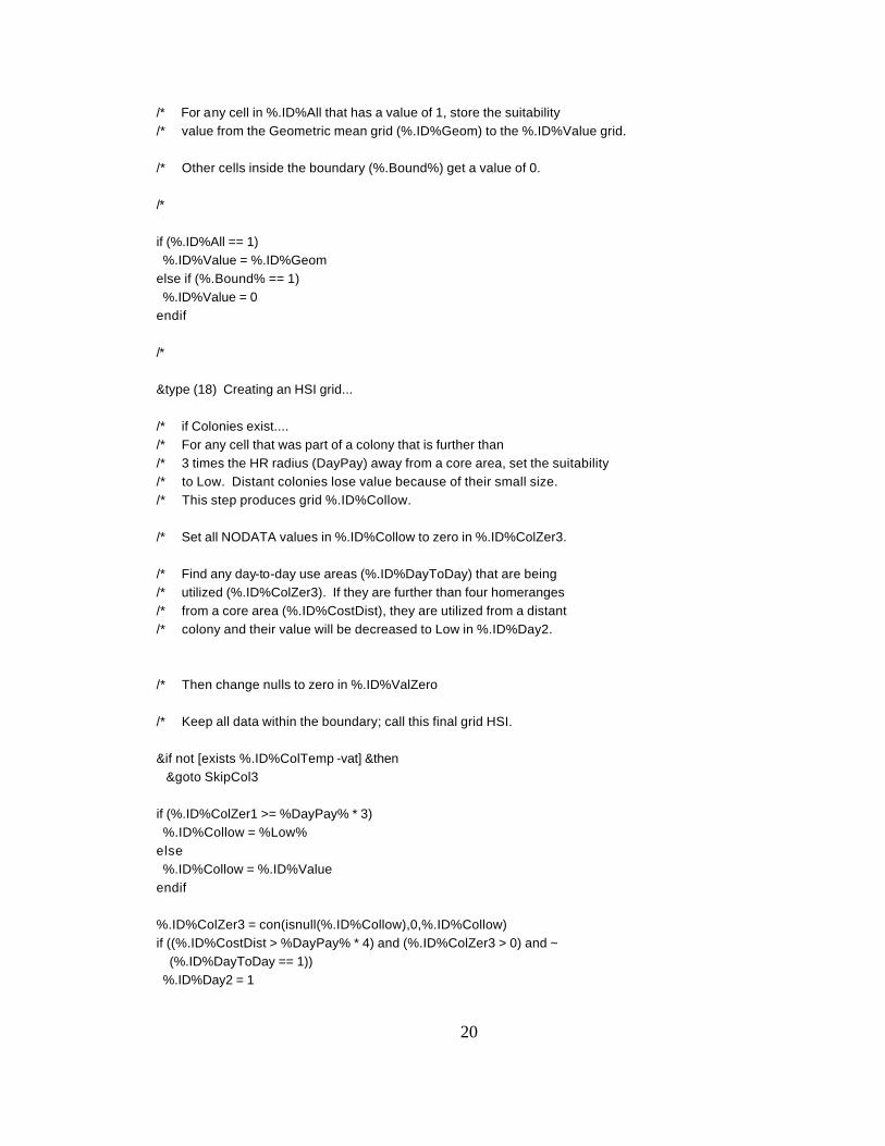
/* For any cell in %.ID%All that has a value of 1, store the suitability /* value from the Geometric mean grid (%.ID%Geom) to the %.ID%Value grid.

/* Other cells inside the boundary (%.Bound%) get a value of 0.

/*

if (%.ID%All == 1) %.ID%Value = %.ID%Geom else if (%.Bound% == 1) %.ID%Value = 0 endif

/*

&type (18) Creating an HSI grid...

/* if Colonies exist..../* For any cell that was part of a colony that is further than

/* 3 times the HR radius (DayPay) away from a core area, set the suitability

/* to Low. Distant colonies lose value because of their small size./* This step produces grid %.ID%Collow.

/* Set all NODATA values in %.ID%Collow to zero in %.ID%ColZer3.

/* Find any day-to-day use areas (%.ID%DayToDay) that are being

/* utilized (%.ID%ColZer3). If they are further than four homeranges

/* from a core area (%.ID%CostDist), they are utilized from a distant/* colony and their value will be decreased to Low in %.ID%Day2.

/* Then change nulls to zero in %.ID%ValZero

/* Keep all data within the boundary; call this final grid HSI.

&if not [exists %.ID%ColTemp -vat] &then &goto SkipCol3

if (%.ID%ColZer1 >= %DayPay% * 3) %.ID%Collow = %Low% else %.ID%Collow = %.ID%Value endif

%.ID%ColZer3 = con(isnull(%.ID%Collow),0,%.ID%Collow) if ((%.ID%CostDist > %DayPay% * 4) and (%.ID%ColZer3 > 0) and ~

(%.ID%DayToDay == 1)) %.ID%Day2 = 1

20

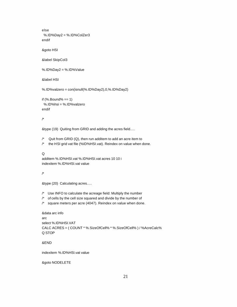
else %.ID%Day2 = %.ID%ColZer3 endif

&goto HSI

&label SkipCol3

%.ID%Day2 = %.ID%Value

&label HSI

%.ID%valzero = con(isnull(%.ID%Day2),0,%.ID%Day2)

if (%.Bound% == 1) %.ID%hsi = %.ID%valzero endif

/*

&type (19) Quiting from GRID and adding the acres field.....

/* Quit from GRID (Q), then run additem to add an acre item to /* the HSI grid vat file (%ID%HSI.vat). Reindex on value when done.

Q additem %.ID%HSI.vat %.ID%HSI.vat acres 10 10 i indexitem %.ID%HSI.vat value

/*

&type (20) Calculating acres.....

/* Use INFO to calculate the acreage field: Multiply the number /* of cells by the cell size squared and divide by the number of /* square meters per acre (4047). Reindex on value when done.

&data arc info arc select %.ID%HSI.VAT CALC ACRES = ( COUNT * %.SizeOfCell% * %.SizeOfCell% ) / %AcreCalc% Q STOP

&END

indexitem %.ID%HSI.vat value

&goto NODELETE

21

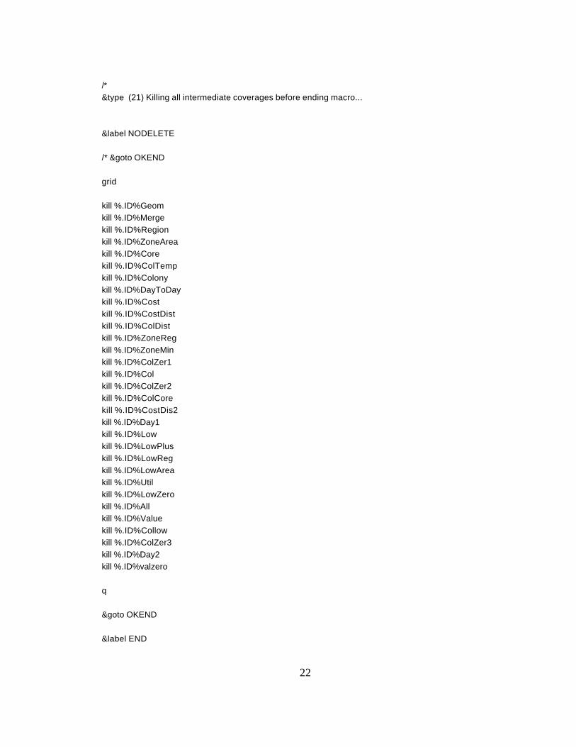
/*&type (21) Killing all intermediate coverages before ending macro...

&label NODELETE

/* &goto OKEND

grid

kill %.ID%Geom

kill %.ID%Merge

kill %.ID%Region

kill %.ID%ZoneArea

kill %.ID%Core

kill %.ID%ColTemp

kill %.ID%Colony

kill %.ID%DayToDay

kill %.ID%Costkill %.ID%CostDistkill %.ID%ColDistkill %.ID%ZoneReg

kill %.ID%ZoneMin

kill %.ID%ColZer1

kill %.ID%Colkill %.ID%ColZer2

kill %.ID%ColCore

kill %.ID%CostDis2

kill %.ID%Day1

kill %.ID%Low

kill %.ID%LowPlus

kill %.ID%LowReg

kill %.ID%LowArea

kill %.ID%Utilkill %.ID%LowZero

kill %.ID%Allkill %.ID%Value

kill %.ID%Collow

kill %.ID%ColZer3

kill %.ID%Day2

kill %.ID%valzero

q

&goto OKEND

&label END

22

&type **

&type **

&type NO CORE AREAS EXIST, EXITING MACRO

&type **

&type **

kill %.ID%Core

kill %.ID%Region

kill %.ID%ZoneArea

kill %.ID%Merge

kill %.ID%Geom

quit

&label OKEND

&type -------------- All done! ----------------

&return

23