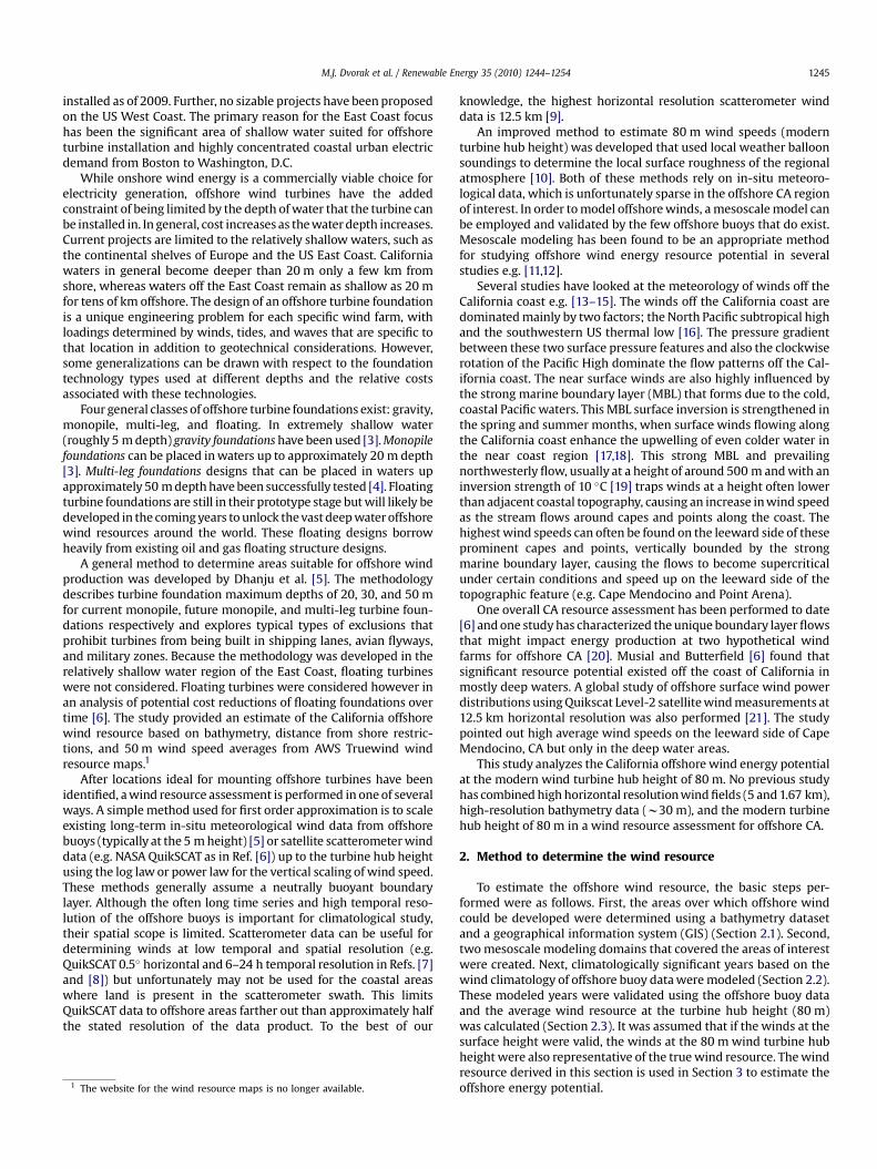
California offshore wind energy potential (Renewable Energy

lable at ScienceDirect

Renewable Energy 35 (2010) 1244–1254

Contents lists avai

Renewable Energy

journal homepage: www.elsevier .com/locate/renene

California offshore wind energy potential

Michael J. Dvorak a,*, Cristina L. Archer b, Mark Z. Jacobson a

a Department of Civil and Environmental Engineering, Stanford University, Stanford, CA, USAb Department of Geological and Environmental Sciences, California State University Chico, Chico, CA, USA

a r t i c l e i n f o

Article history:Received 20 April 2009Accepted 10 November 2009Available online 9 December 2009

Keywords:Offshore wind energyCaliforniaResource assessmentMM5BathymetryMesoscale modeling

* Corresponding author. Atmosphere/Energy ProYamasaki Environment & Energy Building – 4020, StTel.: þ1 650 454 5243; fax: þ1 650 723 7058.

E-mail address: [email protected] (M.J. Dvorak

0960-1481/$ – see front matter � 2009 Elsevier Ltd.doi:10.1016/j.renene.2009.11.022

a b s t r a c t

This study combines multi-year mesoscale modeling results, validated using offshore buoys with high-resolution bathymetry to create a wind energy resource assessment for offshore California (CA). Thesiting of an offshore wind farm is limited by water depth, with shallow water being generally preferableeconomically. Acceptable depths for offshore wind farms are divided into three categories: �20 m depthfor monopile turbine foundations, �50 m depth for multi-leg turbine foundations, and �200 m depth fordeep water floating turbines. The CA coast was further divided into three logical areas for analysis:Northern, Central, and Southern CA. A mesoscale meteorological model was then used at high horizontalresolution (5 and 1.67 km) to calculate annual 80 m wind speeds (turbine hub height) for each area,based on the average of the seasonal months January, April, July, and October of 2005/2006 and theentirety of 2007 (12 months). A 5 MW offshore wind turbine was used to create a preliminary resourceassessment for offshore CA. Each geographical region was then characterized by its coastal transmissionaccess, water depth, wind turbine development potential, and average 80 m wind speed. Initial estimatesshow that 1.4–2.3 GW, 4.4–8.3 GW, and 52.8–64.9 GW of deliverable power could be harnessed fromoffshore CA using monopile, multi-leg, and floating turbine foundations, respectively. A single proposedwind farm near Cape Mendocino could deliver an average 800 MW of gross renewable power and reduceCA’s current carbon emitting electricity generation 4% on an energy basis. Unlike most of California’s landbased wind farms which peak at night, the offshore winds near Cape Mendocino are consistently fastthroughout the day and night during all four seasons.

� 2009 Elsevier Ltd. All rights reserved.

1. Introduction

This paper quantifies the California (CA) offshore wind energyresource using three years of high-resolution mesoscale weathermodeling data, locates shallow offshore areas where turbines couldbe erected using high-resolution bathymetry data, and calculatesthe overall energy and average power that could be obtained fromoffshore wind turbines. Wind power represents the fastest growingrenewable energy resource, growing by 29% in 2008 alone to120,798 MW of installed capacity worldwide. Offshore wind powergrew at an even faster rate of 32% in 2008 with 1471 MW installedexclusively in the seas of Europe but still only represented 1.2% ofthe installed total worldwide [1].

Offshore wind turbines are subject to several additionalconstraints when compared to onshore wind turbines: (1) the cost of

gram, Jerry Yang & Akikoanford, CA 94305-4121, USA.

).

All rights reserved.

mounting the turbine to the sea floor is expensive and limitedcurrently to shallow water depths, (2) undersea electrical trans-mission cable per unit distance is more expensive than overhead-land based transmission lines, (3) offshore weather and waveconditions can cause installation delays as rented equipment isforced to sit idle, and (4) maintenance costs of offshore turbines arehigher. Although offshore wind turbines can be more costly to installand operate, they offer several distinct advantages over their onshorecounterparts: (1) in general, they can be installed closer to coastalurban load centers, where most electrical energy demand exists, (2)transmission constraints and congestion are eased because offshorewind farms can be built closer to load centers, (3) offshore winds arefaster and more consistent at lower vertical heights due to thereduced surface roughness over the ocean, and (4) offshore turbinesand components are not limited by roadway shipping constraints, sohigher capacity turbines can be installed. A detailed cost–benefitanalysis between onshore and offshore wind has been performed [2],highlighting situations where offshore turbines installations areadvantageous to onshore ones.

Although many offshore wind farms have been proposed in theUS particularly off the US East Coast, no offshore turbines have been

M.J. Dvorak et al. / Renewable Energy 35 (2010) 1244–1254 1245

installed as of 2009. Further, no sizable projects have been proposedon the US West Coast. The primary reason for the East Coast focushas been the significant area of shallow water suited for offshoreturbine installation and highly concentrated coastal urban electricdemand from Boston to Washington, D.C.

While onshore wind energy is a commercially viable choice forelectricity generation, offshore wind turbines have the addedconstraint of being limited by the depth of water that the turbine canbe installed in. In general, cost increases as the water depth increases.Current projects are limited to the relatively shallow waters, such asthe continental shelves of Europe and the US East Coast. Californiawaters in general become deeper than 20 m only a few km fromshore, whereas waters off the East Coast remain as shallow as 20 mfor tens of km offshore. The design of an offshore turbine foundationis a unique engineering problem for each specific wind farm, withloadings determined by winds, tides, and waves that are specific tothat location in addition to geotechnical considerations. However,some generalizations can be drawn with respect to the foundationtechnology types used at different depths and the relative costsassociated with these technologies.

Four general classes of offshore turbine foundations exist: gravity,monopile, multi-leg, and floating. In extremely shallow water(roughly 5 m depth) gravity foundations have been used [3]. Monopilefoundations can be placed in waters up to approximately 20 m depth[3]. Multi-leg foundations designs that can be placed in waters upapproximately 50 m depth have been successfully tested [4]. Floatingturbine foundations are still in their prototype stage but will likely bedeveloped in the coming years to unlock the vast deep water offshorewind resources around the world. These floating designs borrowheavily from existing oil and gas floating structure designs.

A general method to determine areas suitable for offshore windproduction was developed by Dhanju et al. [5]. The methodologydescribes turbine foundation maximum depths of 20, 30, and 50 mfor current monopile, future monopile, and multi-leg turbine foun-dations respectively and explores typical types of exclusions thatprohibit turbines from being built in shipping lanes, avian flyways,and military zones. Because the methodology was developed in therelatively shallow water region of the East Coast, floating turbineswere not considered. Floating turbines were considered however inan analysis of potential cost reductions of floating foundations overtime [6]. The study provided an estimate of the California offshorewind resource based on bathymetry, distance from shore restric-tions, and 50 m wind speed averages from AWS Truewind windresource maps.1

After locations ideal for mounting offshore turbines have beenidentified, a wind resource assessment is performed in one of severalways. A simple method used for first order approximation is to scaleexisting long-term in-situ meteorological wind data from offshorebuoys (typically at the 5 m height) [5] or satellite scatterometer winddata (e.g. NASA QuikSCAT as in Ref. [6]) up to the turbine hub heightusing the log law or power law for the vertical scaling of wind speed.These methods generally assume a neutrally buoyant boundarylayer. Although the often long time series and high temporal reso-lution of the offshore buoys is important for climatological study,their spatial scope is limited. Scatterometer data can be useful fordetermining winds at low temporal and spatial resolution (e.g.QuikSCAT 0.5� horizontal and 6–24 h temporal resolution in Refs. [7]and [8]) but unfortunately may not be used for the coastal areaswhere land is present in the scatterometer swath. This limitsQuikSCAT data to offshore areas farther out than approximately halfthe stated resolution of the data product. To the best of our

1 The website for the wind resource maps is no longer available.

knowledge, the highest horizontal resolution scatterometer winddata is 12.5 km [9].

An improved method to estimate 80 m wind speeds (modernturbine hub height) was developed that used local weather balloonsoundings to determine the local surface roughness of the regionalatmosphere [10]. Both of these methods rely on in-situ meteoro-logical data, which is unfortunately sparse in the offshore CA regionof interest. In order to model offshore winds, a mesoscale model canbe employed and validated by the few offshore buoys that do exist.Mesoscale modeling has been found to be an appropriate methodfor studying offshore wind energy resource potential in severalstudies e.g. [11,12].

Several studies have looked at the meteorology of winds off theCalifornia coast e.g. [13–15]. The winds off the California coast aredominated mainly by two factors; the North Pacific subtropical highand the southwestern US thermal low [16]. The pressure gradientbetween these two surface pressure features and also the clockwiserotation of the Pacific High dominate the flow patterns off the Cal-ifornia coast. The near surface winds are also highly influenced bythe strong marine boundary layer (MBL) that forms due to the cold,coastal Pacific waters. This MBL surface inversion is strengthened inthe spring and summer months, when surface winds flowing alongthe California coast enhance the upwelling of even colder water inthe near coast region [17,18]. This strong MBL and prevailingnorthwesterly flow, usually at a height of around 500 m and with aninversion strength of 10 �C [19] traps winds at a height often lowerthan adjacent coastal topography, causing an increase in wind speedas the stream flows around capes and points along the coast. Thehighest wind speeds can often be found on the leeward side of theseprominent capes and points, vertically bounded by the strongmarine boundary layer, causing the flows to become supercriticalunder certain conditions and speed up on the leeward side of thetopographic feature (e.g. Cape Mendocino and Point Arena).

One overall CA resource assessment has been performed to date[6] and one study has characterized the unique boundary layer flowsthat might impact energy production at two hypothetical windfarms for offshore CA [20]. Musial and Butterfield [6] found thatsignificant resource potential existed off the coast of California inmostly deep waters. A global study of offshore surface wind powerdistributions using Quikscat Level-2 satellite wind measurements at12.5 km horizontal resolution was also performed [21]. The studypointed out high average wind speeds on the leeward side of CapeMendocino, CA but only in the deep water areas.

This study analyzes the California offshore wind energy potentialat the modern wind turbine hub height of 80 m. No previous studyhas combined high horizontal resolution wind fields (5 and 1.67 km),high-resolution bathymetry data (w30 m), and the modern turbinehub height of 80 m in a wind resource assessment for offshore CA.

2. Method to determine the wind resource

To estimate the offshore wind resource, the basic steps per-formed were as follows. First, the areas over which offshore windcould be developed were determined using a bathymetry datasetand a geographical information system (GIS) (Section 2.1). Second,two mesoscale modeling domains that covered the areas of interestwere created. Next, climatologically significant years based on thewind climatology of offshore buoy data were modeled (Section 2.2).These modeled years were validated using the offshore buoy dataand the average wind resource at the turbine hub height (80 m)was calculated (Section 2.3). It was assumed that if the winds at thesurface height were valid, the winds at the 80 m wind turbine hubheight were also representative of the true wind resource. The windresource derived in this section is used in Section 3 to estimate theoffshore energy potential.

2 This corresponds to the installation of 45–80% more turbines. This increase is dueto the difference in which offshore areas have the necessary cutoff speed of n80 m of7.0 and 7.5 ms�1 respectively. This energy resource calculation method is explained indetail in Section3.

M.J. Dvorak et al. / Renewable Energy 35 (2010) 1244–12541246

2.1. Offshore areas suitable for development

To estimate the wind resource potential based on depth, thebathymetry data were classified by each type of turbine foundation;0–20 m for monopiles, 20–50 m for multi-leg, and 50–200 m forfloating turbines. These depths are used as turbine foundationconstraints throughout the study and coincide with the depths usedin the offshore wind assessment methodology [5], with the excep-tion that the 30 m ‘‘future’’ monopile class was ignored to simplifythe study and remain consistent with general experience to datewith monopile foundations (as reviewed in the Introduction). Wehave neglected gravity base turbine foundations, due to their limitedutility in CA’s generally deeper water. Deep water floating turbinefoundations were considered for 50–200 m depth, similar to Ref. [6].We only generalize depth classes here to roughly classify thepotential cost and technological requirements of developing windfarms in shallow versus deep water.

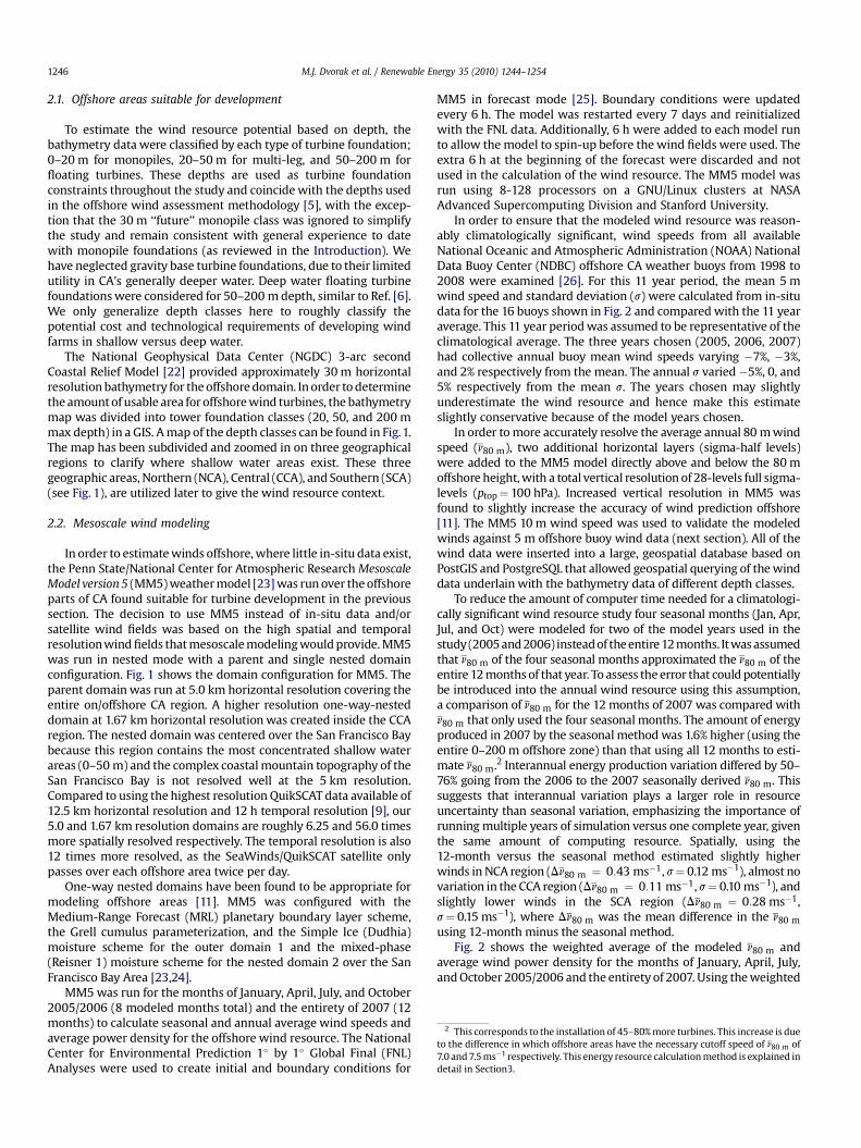
The National Geophysical Data Center (NGDC) 3-arc secondCoastal Relief Model [22] provided approximately 30 m horizontalresolution bathymetry for the offshore domain. In order to determinethe amount of usable area for offshore wind turbines, the bathymetrymap was divided into tower foundation classes (20, 50, and 200 mmax depth) in a GIS. A map of the depth classes can be found in Fig.1.The map has been subdivided and zoomed in on three geographicalregions to clarify where shallow water areas exist. These threegeographic areas, Northern (NCA), Central (CCA), and Southern (SCA)(see Fig. 1), are utilized later to give the wind resource context.

2.2. Mesoscale wind modeling

In order to estimate winds offshore, where little in-situ data exist,the Penn State/National Center for Atmospheric Research MesoscaleModel version 5 (MM5) weather model [23] was run over the offshoreparts of CA found suitable for turbine development in the previoussection. The decision to use MM5 instead of in-situ data and/orsatellite wind fields was based on the high spatial and temporalresolution wind fields that mesoscale modeling would provide. MM5was run in nested mode with a parent and single nested domainconfiguration. Fig. 1 shows the domain configuration for MM5. Theparent domain was run at 5.0 km horizontal resolution covering theentire on/offshore CA region. A higher resolution one-way-nesteddomain at 1.67 km horizontal resolution was created inside the CCAregion. The nested domain was centered over the San Francisco Baybecause this region contains the most concentrated shallow waterareas (0–50 m) and the complex coastal mountain topography of theSan Francisco Bay is not resolved well at the 5 km resolution.Compared to using the highest resolution QuikSCAT data available of12.5 km horizontal resolution and 12 h temporal resolution [9], our5.0 and 1.67 km resolution domains are roughly 6.25 and 56.0 timesmore spatially resolved respectively. The temporal resolution is also12 times more resolved, as the SeaWinds/QuikSCAT satellite onlypasses over each offshore area twice per day.

One-way nested domains have been found to be appropriate formodeling offshore areas [11]. MM5 was configured with theMedium-Range Forecast (MRL) planetary boundary layer scheme,the Grell cumulus parameterization, and the Simple Ice (Dudhia)moisture scheme for the outer domain 1 and the mixed-phase(Reisner 1) moisture scheme for the nested domain 2 over the SanFrancisco Bay Area [23,24].

MM5 was run for the months of January, April, July, and October2005/2006 (8 modeled months total) and the entirety of 2007 (12months) to calculate seasonal and annual average wind speeds andaverage power density for the offshore wind resource. The NationalCenter for Environmental Prediction 1� by 1� Global Final (FNL)Analyses were used to create initial and boundary conditions for

MM5 in forecast mode [25]. Boundary conditions were updatedevery 6 h. The model was restarted every 7 days and reinitializedwith the FNL data. Additionally, 6 h were added to each model runto allow the model to spin-up before the wind fields were used. Theextra 6 h at the beginning of the forecast were discarded and notused in the calculation of the wind resource. The MM5 model wasrun using 8-128 processors on a GNU/Linux clusters at NASAAdvanced Supercomputing Division and Stanford University.

In order to ensure that the modeled wind resource was reason-ably climatologically significant, wind speeds from all availableNational Oceanic and Atmospheric Administration (NOAA) NationalData Buoy Center (NDBC) offshore CA weather buoys from 1998 to2008 were examined [26]. For this 11 year period, the mean 5 mwind speed and standard deviation (s) were calculated from in-situdata for the 16 buoys shown in Fig. 2 and compared with the 11 yearaverage. This 11 year period was assumed to be representative of theclimatological average. The three years chosen (2005, 2006, 2007)had collective annual buoy mean wind speeds varying �7%, �3%,and 2% respectively from the mean. The annual s varied�5%, 0, and5% respectively from the mean s. The years chosen may slightlyunderestimate the wind resource and hence make this estimateslightly conservative because of the model years chosen.

In order to more accurately resolve the average annual 80 m windspeed (n80 m), two additional horizontal layers (sigma-half levels)were added to the MM5 model directly above and below the 80 moffshore height, with a total vertical resolution of 28-levels full sigma-levels (ptop¼ 100 hPa). Increased vertical resolution in MM5 wasfound to slightly increase the accuracy of wind prediction offshore[11]. The MM5 10 m wind speed was used to validate the modeledwinds against 5 m offshore buoy wind data (next section). All of thewind data were inserted into a large, geospatial database based onPostGIS and PostgreSQL that allowed geospatial querying of the winddata underlain with the bathymetry data of different depth classes.

To reduce the amount of computer time needed for a climatologi-cally significant wind resource study four seasonal months (Jan, Apr,Jul, and Oct) were modeled for two of the model years used in thestudy (2005 and 2006) instead of the entire 12 months. It was assumedthat n80 m of the four seasonal months approximated the n80 m of theentire 12 months of that year. To assess the error that could potentiallybe introduced into the annual wind resource using this assumption,a comparison of n80 m for the 12 months of 2007 was compared withn80 m that only used the four seasonal months. The amount of energyproduced in 2007 by the seasonal method was 1.6% higher (using theentire 0–200 m offshore zone) than that using all 12 months to esti-mate n80 m.2 Interannual energy production variation differed by 50–76% going from the 2006 to the 2007 seasonally derived n80 m. Thissuggests that interannual variation plays a larger role in resourceuncertainty than seasonal variation, emphasizing the importance ofrunning multiple years of simulation versus one complete year, giventhe same amount of computing resource. Spatially, using the12-month versus the seasonal method estimated slightly higherwinds in NCA region (Dn80 m ¼ 0:43 ms�1, s¼ 0.12 ms�1), almost novariation in the CCA region (Dn80 m ¼ 0:11 ms�1, s¼ 0.10 ms�1), andslightly lower winds in the SCA region (Dn80 m ¼ 0:28 ms�1,s¼ 0.15 ms�1), where Dn80 m was the mean difference in the n80 musing 12-month minus the seasonal method.

Fig. 2 shows the weighted average of the modeled n80 m andaverage wind power density for the months of January, April, July,and October 2005/2006 and the entirety of 2007. Using the weighted

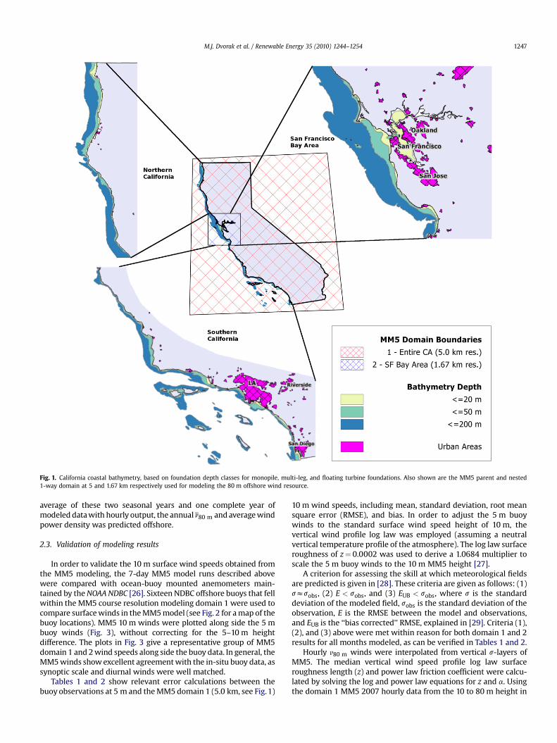
Fig. 1. California coastal bathymetry, based on foundation depth classes for monopile, multi-leg, and floating turbine foundations. Also shown are the MM5 parent and nested1-way domain at 5 and 1.67 km respectively used for modeling the 80 m offshore wind resource.

M.J. Dvorak et al. / Renewable Energy 35 (2010) 1244–1254 1247

average of these two seasonal years and one complete year ofmodeled data with hourly output, the annual n80 m and average windpower density was predicted offshore.

2.3. Validation of modeling results

In order to validate the 10 m surface wind speeds obtained fromthe MM5 modeling, the 7-day MM5 model runs described abovewere compared with ocean-buoy mounted anemometers main-tained by the NOAA NDBC [26]. Sixteen NDBC offshore buoys that fellwithin the MM5 course resolution modeling domain 1 were used tocompare surface winds in the MM5 model (see Fig. 2 for a map of thebuoy locations). MM5 10 m winds were plotted along side the 5 mbuoy winds (Fig. 3), without correcting for the 5–10 m heightdifference. The plots in Fig. 3 give a representative group of MM5domain 1 and 2 wind speeds along side the buoy data. In general, theMM5 winds show excellent agreement with the in-situ buoy data, assynoptic scale and diurnal winds were well matched.

Tables 1 and 2 show relevant error calculations between thebuoy observations at 5 m and the MM5 domain 1 (5.0 km, see Fig. 1)

10 m wind speeds, including mean, standard deviation, root meansquare error (RMSE), and bias. In order to adjust the 5 m buoywinds to the standard surface wind speed height of 10 m, thevertical wind profile log law was employed (assuming a neutralvertical temperature profile of the atmosphere). The log law surfaceroughness of z¼ 0.0002 was used to derive a 1.0684 multiplier toscale the 5 m buoy winds to the 10 m MM5 height [27].

A criterion for assessing the skill at which meteorological fieldsare predicted is given in [28]. These criteria are given as follows: (1)szsobs, (2) E < sobs, and (3) EUB < sobs, where s is the standarddeviation of the modeled field, sobs is the standard deviation of theobservation, E is the RMSE between the model and observations,and EUB is the ‘‘bias corrected’’ RMSE, explained in [29]. Criteria (1),(2), and (3) above were met within reason for both domain 1 and 2results for all months modeled, as can be verified in Tables 1 and 2.

Hourly v80 m winds were interpolated from vertical s-layers ofMM5. The median vertical wind speed profile log law surfaceroughness length (z) and power law friction coefficient were calcu-lated by solving the log and power law equations for z and a. Usingthe domain 1 MM5 2007 hourly data from the 10 to 80 m height in

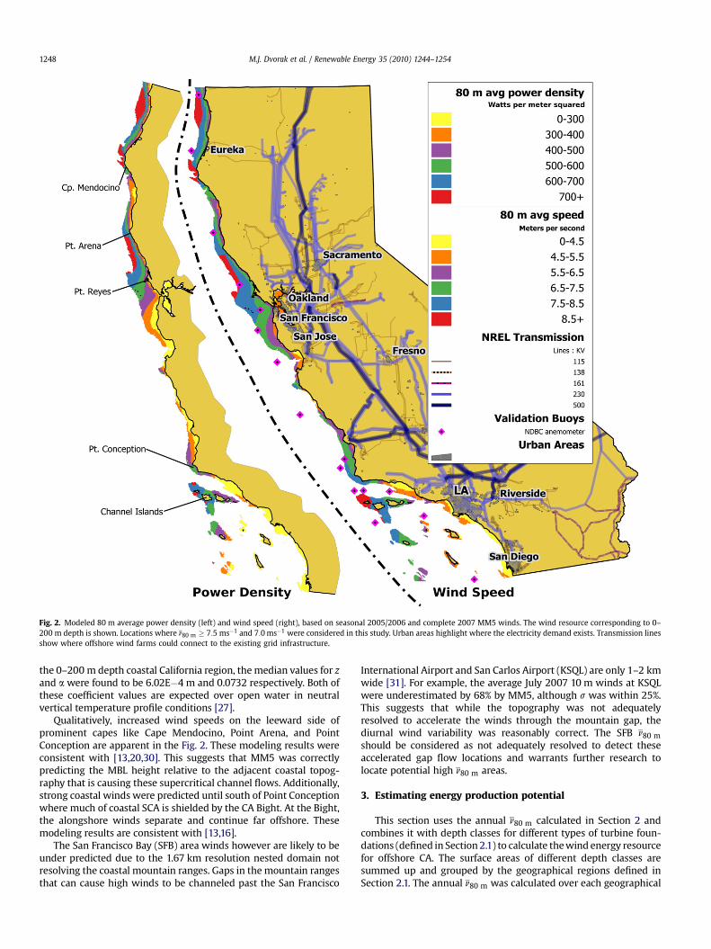
Fig. 2. Modeled 80 m average power density (left) and wind speed (right), based on seasonal 2005/2006 and complete 2007 MM5 winds. The wind resource corresponding to 0–200 m depth is shown. Locations where n80 m � 7:5 ms�1 and 7:0 ms�1 were considered in this study. Urban areas highlight where the electricity demand exists. Transmission linesshow where offshore wind farms could connect to the existing grid infrastructure.

M.J. Dvorak et al. / Renewable Energy 35 (2010) 1244–12541248

the 0–200 m depth coastal California region, the median values for zand a were found to be 6.02E�4 m and 0.0732 respectively. Both ofthese coefficient values are expected over open water in neutralvertical temperature profile conditions [27].

Qualitatively, increased wind speeds on the leeward side ofprominent capes like Cape Mendocino, Point Arena, and PointConception are apparent in the Fig. 2. These modeling results wereconsistent with [13,20,30]. This suggests that MM5 was correctlypredicting the MBL height relative to the adjacent coastal topog-raphy that is causing these supercritical channel flows. Additionally,strong coastal winds were predicted until south of Point Conceptionwhere much of coastal SCA is shielded by the CA Bight. At the Bight,the alongshore winds separate and continue far offshore. Thesemodeling results are consistent with [13,16].

The San Francisco Bay (SFB) area winds however are likely to beunder predicted due to the 1.67 km resolution nested domain notresolving the coastal mountain ranges. Gaps in the mountain rangesthat can cause high winds to be channeled past the San Francisco

International Airport and San Carlos Airport (KSQL) are only 1–2 kmwide [31]. For example, the average July 2007 10 m winds at KSQLwere underestimated by 68% by MM5, although s was within 25%.This suggests that while the topography was not adequatelyresolved to accelerate the winds through the mountain gap, thediurnal wind variability was reasonably correct. The SFB n80 mshould be considered as not adequately resolved to detect theseaccelerated gap flow locations and warrants further research tolocate potential high n80 m areas.

3. Estimating energy production potential

This section uses the annual n80 m calculated in Section 2 andcombines it with depth classes for different types of turbine foun-dations (defined in Section 2.1) to calculate the wind energy resourcefor offshore CA. The surface areas of different depth classes aresummed up and grouped by the geographical regions defined inSection 2.1. The annual n80 m was calculated over each geographical

Fig. 3. 16-Months of representative 10 m height MM5 winds and the 5 m height NDBC buoy winds. The first two rows are from Domain 1 (5 km resolution, CA inclusive) and the lasttwo rows are from Domain 2 (1.67 km resolution, San Francisco Bay Area). Buoy station number and year-month are indicated on each individual. See Fig. 2 for location of the NDBCbuoys.

M.J. Dvorak et al. / Renewable Energy 35 (2010) 1244–1254 1249

region and depth class. Specifications from a representative 5 MWoffshore turbine were used to calculate how many turbines could bebuilt in each region. These turbine specifications were also used tocalculate the capacity factor (CF) over each region/depth class andannual energy/power estimates based on the annual n80 m found ineach region (Section 3.1). The regional implications of the offshorewind energy resource, based on transmission access and electricitydemand are discussed in Section 3.2. Finally, the utility of an examplewind farm in some of the best offshore wind resource and shallowwater is shown (Section 3.3). Hourly power production of the windfarm is explored, to illustrate the potential usefulness of thisresource.

3.1. Calculation of wind resource at different depths

Using the n80 m calculated in Section 2, offshore areas wheren80 m � 7:5 and 7:0 ms�1 were selected for potential turbinedevelopment. The 7.5 ms�1 cutoff was chosen to coincide with theNational Renewable Energy Laboratory (NREL) Class 5 resource,with a average power density of 500 W/m2 [32]. The 7.0 ms�1 cutoffwas chosen to include the future possibility of an offshore windturbine that could utilize lower wind speeds (NREL Class 4). Thegeospatial intersection of the NGDC bathymetry data and the annualmodeled wind resource greater than 7.5 and 7.0 ms�1 is the basis forthe surface areas in Table 3.

To simplify the offshore wind resource assessment, the averagewind speeds were grouped by ocean depth and cutoff wind speed,shown in Table 3. In order to calculate annual energy production,it was necessary to pick a specific turbine model. The REpower5M, 5 MW wind turbine with a 126 diameter at 80 m height waschosen [33]. Although the hub height for the offshore REpower 5M,is 90–100 m, this study used the slightly more conservative 80 mheight. The wind speed would be approximately 1.7% faster atthe 100 m height, based on the vertical wind profile log law(z¼ 0.0002) [27].

In order to determine how much water surface area would berequired for each turbine, a 4-diameter by 7-diameter spacing [27]

was chosen between turbines, where the turbine diameter is126 m. Each REpower 5M turbine would require 0.44 km2 of areaper turbine. In order to account for the water surface area thatwould potentially be unusable due to shipping lanes, restrictedwildlife preservation areas, viewshed considerations, etc., a 33%exclusionary factor for all possible turbine areas was included ineach nameplate capacity and energy calculation. We used a 33%exclusionary factor in lieu of a complete exclusion zone assessmentbased on a study by Kempton et al. [34]. That study found that thesum of the avian flyways, waste areas, beach nourishment borrowareas, and shipping lanes was 35% of the available water area from0 to 40 m and 10% at the 50–100 m depth waters, making our 33%exclusionary factor conservative for the mostly deep Californiaoffshore areas. Future studies should look at the details of eacharea’s exclusion zones, in order to more precisely calculate amountof usable surface area. Table 4 shows the nameplate capacity of eachgeographical region and depth class.

The n80 m calculated in the previous section was used to deter-mine turbine CF, which in turn yielded an annual energy andaverage power output at each offshore site with suitable windresource and shallow water. The CFs for the proposed wind farmswere estimated using Eq. (1)

Capacity Factor ¼ 0:087� Vavgðm=sÞ � PratedðkWÞD2ðmÞ

(1)

which states the relationship between mean wind speed (Vavg),rated power (Prated) and rotor diameter (D) [27], using the turbinedimensions for the REpower 5M turbine. This equation has beenshown to apply to a wide variety of wind turbine types [35] and wasalso utilized in three wind resource studies [20,35,36].

We have assumed a Rayleigh distribution over time of winds atthe 80 m hub height by using the CF Eq. (1) explained in [27]. Theerror of using Eq. (1) to calculate CF was estimated by integratingthe hourly power output from the REpower 5M turbine for all theMM5 model data from 2007 in the 0–200 m depth region. Usingdomain 1 (see Fig. 1) grid points where n80 m � 7:5 ms�1 corre-sponding to NREL Class 5 winds (500–600 Wm�2), the CF method

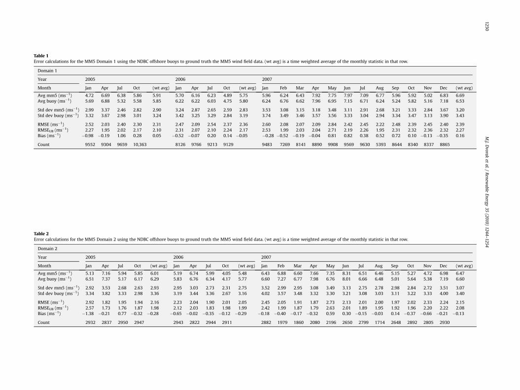
Table 1Error calculations for the MM5 Domain 1 using the NDBC offshore buoys to ground truth the MM5 wind field data. (wt avg) is a time weighted average of the monthly statistic in that row.

Domain 1

Year 2005 2006 2007

Month Jan Apr Jul Oct (wt avg) Jan Apr Jul Oct (wt avg) Jan Feb Mar Apr May Jun Jul Aug Sep Oct Nov Dec (wt avg)

Avg mm5 (ms�1) 4.72 6.69 6.38 5.86 5.91 5.70 6.16 6.23 4.89 5.75 5.96 6.24 6.43 7.92 7.75 7.97 7.09 6.77 5.96 5.92 5.02 6.83 6.69Avg buoy (ms�1) 5.69 6.88 5.32 5.58 5.85 6.22 6.22 6.03 4.75 5.80 6.24 6.76 6.62 7.96 6.95 7.15 6.71 6.24 5.24 5.82 5.16 7.18 6.53

Std dev mm5 (ms�1) 2.99 3.37 2.46 2.82 2.90 3.24 2.87 2.65 2.59 2.83 3.53 3.08 3.15 3.18 3.48 3.11 2.91 2.68 3.21 3.33 2.84 3.67 3.20Std dev buoy (ms�1) 3.32 3.67 2.98 3.01 3.24 3.42 3.25 3.29 2.84 3.19 3.74 3.49 3.46 3.57 3.56 3.33 3.04 2.94 3.34 3.47 3.13 3.90 3.43

RMSE (ms�1) 2.52 2.03 2.40 2.30 2.31 2.47 2.09 2.54 2.37 2.36 2.60 2.08 2.07 2.09 2.84 2.42 2.45 2.22 2.48 2.39 2.45 2.40 2.39RMSEUB (ms�1) 2.27 1.95 2.02 2.17 2.10 2.31 2.07 2.10 2.24 2.17 2.53 1.99 2.03 2.04 2.71 2.19 2.26 1.95 2.31 2.32 2.36 2.32 2.27Bias (ms�1) �0.98 �0.19 1.06 0.28 0.05 �0.52 �0.07 0.20 0.14 �0.05 �0.28 �0.52 �0.19 �0.04 0.81 0.82 0.38 0.52 0.72 0.10 �0.13 �0.35 0.16

Count 9552 9304 9659 10,363 8126 9766 9213 9129 9483 7269 8141 8890 9908 9569 9630 5393 8644 8340 8337 8865

Table 2Error calculations for the MM5 Domain 2 using the NDBC offshore buoys to ground truth the MM5 wind field data. (wt avg) is a time weighted average of the monthly statistic in that row.

Domain 2

Year 2005 2006 2007

Month Jan Apr Jul Oct (wt avg) Jan Apr Jul Oct (wt avg) Jan Feb Mar Apr May Jun Jul Aug Sep Oct Nov Dec (wt avg)

Avg mm5 (ms�1) 5.13 7.16 5.94 5.85 6.01 5.19 6.74 5.99 4.05 5.48 6.43 6.88 6.60 7.66 7.35 8.31 6.51 6.46 5.15 5.27 4.72 6.98 6.47Avg buoy (ms�1) 6.51 7.37 5.17 6.17 6.29 5.83 6.76 6.34 4.17 5.77 6.60 7.27 6.77 7.98 6.76 8.01 6.66 6.48 5.01 5.64 5.38 7.19 6.60

Std dev mm5 (ms�1) 2.92 3.53 2.68 2.63 2.93 2.95 3.03 2.73 2.31 2.75 3.52 2.99 2.95 3.08 3.49 3.13 2.75 2.78 2.98 2.84 2.72 3.51 3.07Std dev buoy (ms�1) 3.34 3.82 3.33 2.98 3.36 3.19 3.44 3.36 2.67 3.16 4.02 3.57 3.48 3.32 3.30 3.21 3.08 3.03 3.11 3.22 3.33 4.00 3.40

RMSE (ms�1) 2.92 1.82 1.95 1.94 2.16 2.23 2.04 1.90 2.01 2.05 2.45 2.05 1.91 1.87 2.73 2.13 2.01 2.00 1.97 2.02 2.33 2.24 2.15RMSEUB (ms�1) 2.57 1.73 1.76 1.87 1.98 2.12 2.03 1.83 1.98 1.99 2.42 1.99 1.87 1.79 2.63 2.01 1.89 1.95 1.92 1.96 2.20 2.22 2.08Bias (ms�1) �1.38 �0.21 0.77 �0.32 �0.28 �0.65 �0.02 �0.35 �0.12 �0.29 �0.18 �0.40 �0.17 �0.32 0.59 0.30 �0.15 �0.03 0.14 �0.37 �0.66 �0.21 �0.13

Count 2932 2837 2950 2947 2943 2822 2944 2911 2882 1979 1860 2080 2196 2650 2799 1714 2648 2892 2805 2930

M.J.D

voraket

al./Renew

ableEnergy

35(2010)

1244–12541250

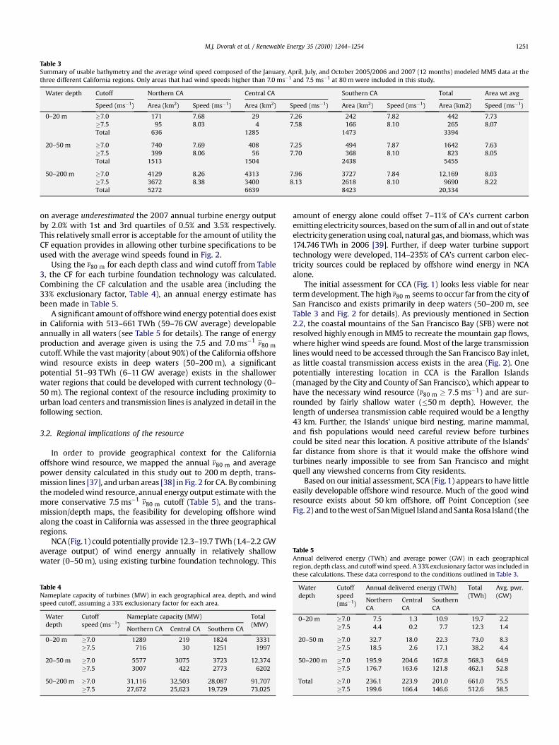
Table 3Summary of usable bathymetry and the average wind speed composed of the January, April, July, and October 2005/2006 and 2007 (12 months) modeled MM5 data at thethree different California regions. Only areas that had wind speeds higher than 7.0 ms�1 and 7.5 ms�1 at 80 m were included in this study.

Water depth Cutoff Northern CA Central CA Southern CA Total Area wt avg

Speed (ms�1) Area (km2) Speed (ms�1) Area (km2) Speed (ms�1) Area (km2) Speed (ms�1) Area (km2) Speed (ms�1)

0–20 m �7.0 171 7.68 29 7.26 242 7.82 442 7.73�7.5 95 8.03 4 7.58 166 8.10 265 8.07Total 636 1285 1473 3394

20–50 m �7.0 740 7.69 408 7.25 494 7.87 1642 7.63�7.5 399 8.06 56 7.70 368 8.10 823 8.05Total 1513 1504 2438 5455

50–200 m �7.0 4129 8.26 4313 7.96 3727 7.84 12,169 8.03�7.5 3672 8.38 3400 8.13 2618 8.10 9690 8.22Total 5272 6639 8423 20,334

Table 5Annual delivered energy (TWh) and average power (GW) in each geographicalregion, depth class, and cutoff wind speed. A 33% exclusionary factor was included in

M.J. Dvorak et al. / Renewable Energy 35 (2010) 1244–1254 1251

on average underestimated the 2007 annual turbine energy outputby 2.0% with 1st and 3rd quartiles of 0.5% and 3.5% respectively.This relatively small error is acceptable for the amount of utility theCF equation provides in allowing other turbine specifications to beused with the average wind speeds found in Fig. 2.

Using the n80 m for each depth class and wind cutoff from Table3, the CF for each turbine foundation technology was calculated.Combining the CF calculation and the usable area (including the33% exclusionary factor, Table 4), an annual energy estimate hasbeen made in Table 5.

A significant amount of offshore wind energy potential does existin California with 513–661 TWh (59–76 GW average) developableannually in all waters (see Table 5 for details). The range of energyproduction and average given is using the 7.5 and 7.0 ms�1 n80 mcutoff. While the vast majority (about 90%) of the California offshorewind resource exists in deep waters (50–200 m), a significantpotential 51–93 TWh (6–11 GW average) exists in the shallowerwater regions that could be developed with current technology (0–50 m). The regional context of the resource including proximity tourban load centers and transmission lines is analyzed in detail in thefollowing section.

3.2. Regional implications of the resource

In order to provide geographical context for the Californiaoffshore wind resource, we mapped the annual n80 m and averagepower density calculated in this study out to 200 m depth, trans-mission lines [37], and urban areas [38] in Fig. 2 for CA. By combiningthe modeled wind resource, annual energy output estimate with themore conservative 7.5 ms�1 n80 m cutoff (Table 5), and the trans-mission/depth maps, the feasibility for developing offshore windalong the coast in California was assessed in the three geographicalregions.

NCA (Fig.1) could potentially provide 12.3–19.7 TWh (1.4–2.2 GWaverage output) of wind energy annually in relatively shallowwater (0–50 m), using existing turbine foundation technology. This

Table 4Nameplate capacity of turbines (MW) in each geographical area, depth, and windspeed cutoff, assuming a 33% exclusionary factor for each area.

Waterdepth

Cutoffspeed (ms�1)

Nameplate capacity (MW) Total(MW)

Northern CA Central CA Southern CA

0–20 m �7.0 1289 219 1824 3331�7.5 716 30 1251 1997

20–50 m �7.0 5577 3075 3723 12,374�7.5 3007 422 2773 6202

50–200 m �7.0 31,116 32,503 28,087 91,707�7.5 27,672 25,623 19,729 73,025

amount of energy alone could offset 7–11% of CA’s current carbonemitting electricity sources, based on the sum of all in and out of stateelectricity generation using coal, natural gas, and biomass, which was174.746 TWh in 2006 [39]. Further, if deep water turbine supporttechnology were developed, 114–235% of CA’s current carbon elec-tricity sources could be replaced by offshore wind energy in NCAalone.

The initial assessment for CCA (Fig. 1) looks less viable for nearterm development. The high n80 m seems to occur far from the city ofSan Francisco and exists primarily in deep waters (50–200 m, seeTable 3 and Fig. 2 for details). As previously mentioned in Section2.2, the coastal mountains of the San Francisco Bay (SFB) were notresolved highly enough in MM5 to recreate the mountain gap flows,where higher wind speeds are found. Most of the large transmissionlines would need to be accessed through the San Francisco Bay inlet,as little coastal transmission access exists in the area (Fig. 2). Onepotentially interesting location in CCA is the Farallon Islands(managed by the City and County of San Francisco), which appear tohave the necessary wind resource (n80 m � 7:5 ms�1) and are sur-rounded by fairly shallow water (�50 m depth). However, thelength of undersea transmission cable required would be a lengthy43 km. Further, the Islands’ unique bird nesting, marine mammal,and fish populations would need careful review before turbinescould be sited near this location. A positive attribute of the Islands’far distance from shore is that it would make the offshore windturbines nearly impossible to see from San Francisco and mightquell any viewshed concerns from City residents.

Based on our initial assessment, SCA (Fig. 1) appears to have littleeasily developable offshore wind resource. Much of the good windresource exists about 50 km offshore, off Point Conception (seeFig. 2) and to the west of San Miguel Island and Santa Rosa Island (the

these calculations. These data correspond to the conditions outlined in Table 3.

Waterdepth

Cutoffspeed(ms�1)

Annual delivered energy (TWh) Total(TWh)

Avg. pwr.(GW)

NorthernCA

CentralCA

SouthernCA

0–20 m �7.0 7.5 1.3 10.9 19.7 2.2�7.5 4.4 0.2 7.7 12.3 1.4

20–50 m �7.0 32.7 18.0 22.3 73.0 8.3�7.5 18.5 2.6 17.1 38.2 4.4

50–200 m �7.0 195.9 204.6 167.8 568.3 64.9�7.5 176.7 163.6 121.8 462.1 52.8

Total �7.0 236.1 223.9 201.0 661.0 75.5�7.5 199.6 166.4 146.6 512.6 58.5

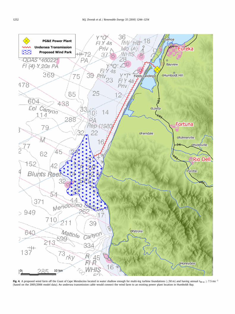
Fig. 4. A proposed wind farm off the Coast of Cape Mendocino located in water shallow enough for multi-leg turbine foundations (�50 m) and having annual n80 m � 7:5 ms�1

(based on the 2005/2006 model data). An undersea transmission cable would connect the wind farm to an existing power plant location in Humboldt Bay.

M.J. Dvorak et al. / Renewable Energy 35 (2010) 1244–12541252

M.J. Dvorak et al. / Renewable Energy 35 (2010) 1244–1254 1253

Channel Islands). Winds south and east of Point Conception aresignificantly reduced. Although alongshore coastal winds flowstrongly until Point Conception, much of SCA is shielded by the CABight, where the alongshore winds separate and continue faroffshore, leaving the Los Angeles area with little coastal wind. Itshould be noted however that the SCA coast does provide severalexcellent grid interconnection points and significant electricaldemand.

3.3. Example offshore wind farm

To illustrate the possible utility that an offshore wind farm couldprovide to the California grid, an example offshore wind farm wascreated, located off Cape Mendocino (see map in Fig. 4). The proposedwind farm is located in water �50 m deep and could be developedtoday with existing turbine foundation technologies. Eureka is anidea location for this project because some existing (albeit small)115 kV power lines cross the coastal mountains eastward to the maintransmission corridor in the California central valley. Additionally, anexisting power plant in Humboldt Bay would provide an ideal loca-tion to connect the sea transmission to the local electric grid.

The annual n80 m calculated using the January, April, July, andOctober 2005/2006 80 m wind speeds from MM5 (8 modeledmonths total) was 8.23 ms�1, which corresponds to a 40% CF usingEq. (1) with the REpower 5M turbine. The wind farm would be mostactive however during the summer months, when the average 80 mwind speed calculated from the July 2005 and 2006 MM5 data is9.67 ms�1; a 53% CF during the summer months using Eq. (1) withthe REpower 5M turbine.

The time of day when wind power peaks is important because thesummer peak electric demand occurs late in the afternoon, around5:00 pm [40]. Electricity generated during peak demand periods ismore valuable than electricity generated during off peak periods,both for air pollution emissions reductions and monetary value. Inorder to analyze how offshore wind power might fit into the Cal-ifornia electric grid, n80 m winds were averaged by hour over theeight seasonal months of the 2005/2006 MM5 model data andshown in Fig. 5. The summertime winds, denoted by the ‘‘July’’ line inFig. 5 are fast and consistent throughout the day. These summer

July

OctoberJanuary

April

Cape Mendocino

hour of day (PST)

0 4 8 12 16 20 24

80-m

win

d sp

eed

(m/s

)

11

10

9

8

7

6

Fig. 5. Mean n80 m winds group by hour of the day (PST) for the proposed wind farmoff the NCA coast (Fig. 4), based on the MM5 output for the 2005/2006 months ofJanuary, April, July, and October.

winds would dovetail extremely well with California electricitydemand during the summer months. Unlike most California landbased wind farms which peak at night, the offshore winds off CapeMendocino are consistent throughout the day during the summermonths [24].

The proposed Cape Mendocino wind farm is 138 km2 and couldaccommodate approximately 300 REpower 5M 5.0 MW wind turbines,with a total project rated capacity of 1500 MW (using a 4-diameterby 7-diameter turbine spacing, as well as a 33% exclusionary factor).The clean energy contribution of this wind farm would be quitesignificant in cleaning California’s electricity supply. The annualenergy output from this project alone could be 6.91 TWh annually,corresponding to an average power output of 790 MW. This windfarm alone could replace 4.0% (gross) of California’s current carbonemitting electric generation (using the carbon emitting electricitygeneration from in and out of state resources of 174.746 TWh in 2006from [39]).

4. Conclusions

Despite the steep bathymetry off the California (CA) coast,significant development potential exists for offshore wind energy. Bylooking at the depth of the water more closely, with a higher reso-lution bathymetry dataset, it was possible to find some areas thatwere previously overlooked for offshore wind power development.This study also qualitatively looked at transmission capacity andpopulation centers to build a context for the offshore wind resourcein CA. It was found that Northern California (NCA) had the best 80 mwind resource but the least transmission capacity compared to otherparts of the state. Some NCA’s resource could be developed today,using existing turbine foundation technology.

Central California will likely require the development of floatingturbines for large scale offshore wind development. Some shallowwater area (�50 m) with good wind resource potential does existnear the Farallon Islands however. The relatively shallow SanFrancisco Bay was not resolved highly enough in the mesoscalemodel to draw conclusive results and warrants further investigation.

The Southern California (SCA) region will more than likely requirethe development of floating turbines for large scale offshore turbinedevelopment. Most of the viable wind resource exists far offshore indeep water and would require lengthy undersea transmission lines.

In sum, including all current and future turbine foundationtechnologies (0–200 m depth), based on the n80 m wind speedcutoffs of 7.5 ms�1 and 7.0 ms�1 between 174% and 224% respec-tively of CA electricity needs (including in-state plus importedgeneration, 294.865 TWh in 2006) could be provided with offshorewind energy alone [39]. Using only currently available turbine towersupport technologies (0–50 m depth), between 17% and 31%respectively of CA electricity need could be provided.

An example wind farm was proposed near Cape Mendocino andthe city of Eureka in water shallow enough to develop offshore windturbines with existing turbine foundation technology. This1500 MW, 300 turbine wind farm located in some of the best Cal-ifornia offshore wind resource could replace up to 4.0% of its currentcarbon emitting electricity generation sources and would delivernearly 800 MW of deliverable renewable power on average. Unlikemost of California land based wind farms which peak at night, theoffshore winds near Cape Mendocino are consistently fast duringday and night for all four seasons.

Acknowledgments

We would like to thank (in alphabetical order) James Doyle,Crystal Dvorak, Jeffery Greenblatt, Tracy Haack, Nick Jenkins, Qing-fang Jiang, Willett Kempton, Martin Ralph, and Zachary Westgate for

M.J. Dvorak et al. / Renewable Energy 35 (2010) 1244–12541254

helpful comments. We would also like to thank John Taylor, forassistance with the MM5 modeling. Thank you to the NationalAeronautics and Space Administration (NASA) Advanced Super-computing (NAS) Division and National Center for AtmosphericResearch’s (NCAR) Computational & Information Systems Laboratory(CISL) for access to computational resources and global weatherdatasets respectively, used in the mesoscale modeling. Support forthis work came from NASA, the Charles H. Leavell Fellowship, andPrecourt Energy Efficiency Center.

References

[1] Global Wind Energy Council. Global wind 2008 report. Available from: http://www.gwec.net/fileadmin/documents/Publications/Report_2008/Global_Wind_2008_Report.pdf; 2009.

[2] Snyder B, Kaiser MJ. Ecological and economic cost–benefit analysis of offshorewind energy. Renewable Energy 2009;34:1567–78.

[3] Henderson AR, Morgan C, Smith B, Sorensen HC, Barthelmie RJ, Boesmans B.Offshore wind energy in Europe – a review of the state-of-the-art. WindEnergy 2003;6:35–52.

[4] Talisman Energy. Beatrice wind farm demonstrator project. Available from:http://www.beatricewind.co.uk/Uploads/Downloads/BEATRICE_WINDFARM.pdf; 2006 [accessed 24.01.07].

[5] Dhanju A, Whitaker P, Kempton W. Assessing offshore wind resources: anaccessible methodology. Renew Energy 2008;33:55–64.

[6] Musial W, Butterfield S. Future for offshore wind energy in the United States.In: Proc. of EnergyOcean 2004. Available from: http://www.nrel.gov/docs/fy04osti/36313.pdf; 2004.

[7] Sørensen B. A new method for estimating off-shore wind potentials. Inter-national Journal of Green Energy 2008;5:139–47.

[8] Pimenta F, Kempton W, Garvine R. Combining meteorological stations andsatellite data to evaluate the offshore wind power resource of SoutheasternBrazil. Renewable Energy 2008;33:2375–87.

[9] Jet Propulsion Laboratory. Available from: QuikSCAT science data productuser’s manual, D-18053-Rev A. Available from: ftp://podaac.jpl.nasa.gov/ocean_wind/quikscat/L2B12/doc/QSUG_v3.pdf; 2006.

[10] Archer CL, Jacobson MZ. Spatial and temporal distributions of U.S. winds andwind power at 80 m derived from measurements. Journal of GeophysicalResearch 2003;108:4289.

[11] Beran J, Claveri L, Lange B, von Bremen L. Offshore wind modelling and forecast.In: Proc. of the 6th WRF/15th MM5 users’ workshop. Available from: http://www.mmm.ucar.edu/wrf/users/workshops/WS2005/abstracts/Session3/30-Beran.pdf; 2005.

[12] Jimenez B, Durante F, Lange B, Kreutzer T, Tambke J. Offshore wind resourceassessment with WAsP and MM5: comparative study for the German Bight.Wind Energy 2007;10:121–34.

[13] Dorman C, Winant C. Buoy observations of the atmosphere along the westcoast of the United States, 1981–1990. Journal of Geophysical Research1995;100:16029.

[14] Archer CL, Jacobson MZ, Ludwig FL. The Santa Cruz eddy. Part I: observationsand statistics. Monthly Weather Review 2005;133:767.

[15] Haack T, Burk SD, Hodur RM. U.S. west coast surface heat fluxes, wind stress,and wind stress curl from a mesoscale model. Monthly Weather Review2005;133:3202–16.

[16] Halliwell GR. The large-scale coastal wind field along the west coast of NorthAmerica 1981–1982. Journal of Geophysical Research 1987;92:1861.

[17] Beardsley RC. Local atmospheric forcing during the coastal ocean dynamicsexperiment 1. A description of the marine boundary layer and atmospheric

conditions over a northern California upwelling region. Journal of GeophysicalResearch 1987;92:1467.

[18] Taylor SV, Cayan DR, Graham NE, Georgakakos KP. Northerly surface windsover the eastern North Pacific Ocean in spring and summer. Journal ofGeophysical Research 2008;113:D02110.

[19] Ralph FM, Neiman PJ, Persson POG, Bane JM, Cancillo ML, Wilczak JM, et al.Kelvin waves and internal bores in the marine boundary layer inversion andtheir relationship to coastally trapped wind reversals. Monthly WeatherReview 2000;128:283–300.

[20] Jiang Q, Doyle JD, Haack T, Dvorak MJ, Archer CL, Jacobson MZ. Exploring windenergy potential off the California coast. Geophysical Research Letters2008;35:L20819.

[21] Liu WT, Tang W, Xie X. Wind power distribution over the ocean. GeophysicalResearch Letters 2008;35.

[22] National Oceanographic and Atmospheric Administration, NationalGeophysical Data Center. National geophysical data center coastal reliefmodel, 3-arc second. Available from: http://www.ngdc.noaa.gov/mgg/coastal/coastal.html; 2000.

[23] Grell GA, Dudhia J, Stauffer DR. A description of the fifth-generation PennState/NCAR mesoscale model (MM5); 1994. p. 117.

[24] Fripp M, Wiser R. Analyzing the effects of temporal wind patterns on the valueof wind-generated electricity at different sites in California and the Northwest,LBNL-60152; 2006.

[25] National Center for Environmental Prediction. NCEP global troposphericanalyses, 1�1, daily 15 Sep 1999–present (ds083.2); 2007.

[26] National Oceanic and Atmospheric Administration, National Data BuoyCenter; 2008.

[27] Masters GM. Renewable and efficient electric power systems. Hoboken, NJ:John Wiley & Sons; 2004.

[28] Pielke Sr RA. Mesoscale meteorological modeling. San Diego: AcademicPress; 2002.

[29] Keyser D, Anthes RA. The applicability of a mixed-layer model of the planetaryboundary layer to real-data forecasting. Monthly Weather Review1977;105:1351–71.

[30] Winant CD, Dorman CE, Friehe CA, Beardsley RC. The marine layer offNorthern California: an example of supercritical channel flow. Journal of theAtmospheric Sciences 1988;45:3588–605.

[31] Gilliam H. Weather of the San Francisco Bay region. Berkeley: University ofCalifornia Press; 2002.

[32] Elliot D, Schwartz M. Development and validation of high-resolution statewind resource maps for the United States. NREL/TP-500-38127. Availablefrom: http://www.nrel.gov/docs/fy05osti/38127.pdf; 2005.

[33] REpower Sytems AG. REpower systems AG: 5 M goes offshore: the countdownis running. Available from: http://www.repower.de/index.php?id¼369&L¼1;2007 [accessed 15.06.07].

[34] Kempton W, Archer CL, Dhanju A, Garvine RW, Jacobson MZ. Large CO2reductions via offshore wind power matched to inherent storage in energyend-uses. Geophysical Research Letters 2007;34:2817.

[35] Archer CL, Jacobson MZ. Evaluation of global wind power. Journal ofGeophysical Research 2005;110:1.

[36] Yue C, Yang M. Exploring the potential of wind energy for a coastal state.Energy Policy 2009;37:3925–40.

[37] Federal Emergency Management Agency. Transmission lines for conterminousUnited States (115 kV and above). Distributed by the National Renewable EnergyLaboratory. Available from: http://www.nrel.gov/gis/data_analysis.html; 1993.

[38] U.S. Geological Survey. Urban areas of the United States. Available from: http://nationalatlas.gov/mld/urbanap.html; 2001.

[39] California Energy Commission. 2006 Net system power report. Available from:http://www.energy.ca.gov/2007publications/CEC-300-2007-007/CEC-300-2007-007.PDF; 2007 [accessed 22.10.09].

[40] Price H, Cable R. Parabolic trough power for the California competitive market.Available from: http://www.p2pays.org/ref/18/17978.pdf; 2001.