An Introduction to Acoustics S.W. Rienstra & A. Hirschberg Eindhoven University of Technology 22 January 2012 This is an extended and revised edition of IWDE 92-06. Comments and corrections are gratefully accepted. This file may be used and printed, but for personal or educational purposes only. c S.W. Rienstra & A. Hirschberg 2004.

Welcome message from author
This document is posted to help you gain knowledge. Please leave a comment to let me know what you think about it! Share it to your friends and learn new things together.
Transcript

An Introduction to Acoustics
S.W. Rienstra & A. HirschbergEindhoven University of Technology
22 January 2012
This is an extended and revised edition of IWDE 92-06.
Comments and corrections are gratefully accepted.
This file may be used and printed, but for personal or educational purposes only.
c© S.W. Rienstra & A. Hirschberg 2004.


Contents
Preface
1 Some fluid dynamics 1
1.1 Conservation laws and constitutive equations. . . . . . . . . . . . . . . . . . . . . 1
1.2 Approximations and alternative forms of the conservation laws for ideal fluids. . . . . 4
2 Wave equation, speed of sound, and acoustic energy 8
2.1 Order of magnitude estimates. . . . . . . . . . . . . . . . . . . . . . . . . . . . . 8
2.2 Wave equation for a uniform stagnant fluid and compactness . . . . . . . . . . . . . 11
2.2.1 Linearization and wave equation. . . . . . . . . . . . . . . . . . . . . . . . 11
2.2.2 Simple solutions. . . . . . . . . . . . . . . . . . . . . . . . . . . . . . . . . 13
2.2.3 Compactness. . . . . . . . . . . . . . . . . . . . . . . . . . . . . . . . . . 14
2.3 Speed of sound. . . . . . . . . . . . . . . . . . . . . . . . . . . . . . . . . . . . . 15
2.3.1 Ideal gas. . . . . . . . . . . . . . . . . . . . . . . . . . . . . . . . . . . . . 15
2.3.2 Water . . . . . . . . . . . . . . . . . . . . . . . . . . . . . . . . . . . . . . 16
2.3.3 Bubbly liquid at low frequencies. . . . . . . . . . . . . . . . . . . . . . . . 16
2.4 Influence of temperature gradient. . . . . . . . . . . . . . . . . . . . . . . . . . . 18
2.5 Influence of mean flow. . . . . . . . . . . . . . . . . . . . . . . . . . . . . . . . . 19
2.6 Sources of sound. . . . . . . . . . . . . . . . . . . . . . . . . . . . . . . . . . . . 19
2.6.1 Inverse problem and uniqueness of sources. . . . . . . . . . . . . . . . . . . 19
2.6.2 Mass and momentum injection. . . . . . . . . . . . . . . . . . . . . . . . . 20
2.6.3 Lighthill’s analogy . . . . . . . . . . . . . . . . . . . . . . . . . . . . . . . 21
2.6.4 Vortex sound . . . . . . . . . . . . . . . . . . . . . . . . . . . . . . . . . . 24
2.7 Acoustic energy . . . . . . . . . . . . . . . . . . . . . . . . . . . . . . . . . . . . 25
2.7.1 Introduction. . . . . . . . . . . . . . . . . . . . . . . . . . . . . . . . . . . 25
2.7.2 Kirchhoff’s equation for quiescent fluids. . . . . . . . . . . . . . . . . . . . 26
2.7.3 Acoustic energy in a non-uniform flow. . . . . . . . . . . . . . . . . . . . . 29
2.7.4 Acoustic energy and vortex sound. . . . . . . . . . . . . . . . . . . . . . . . 30
ii Contents
3 Green’s functions, impedance, and evanescent waves 33
3.1 Green’s functions. . . . . . . . . . . . . . . . . . . . . . . . . . . . . . . . . . . . 33
3.1.1 Integral representations. . . . . . . . . . . . . . . . . . . . . . . . . . . . . 33
3.1.2 Remarks on finding Green’s functions. . . . . . . . . . . . . . . . . . . . . . 35
3.2 Acoustic impedance . . . . . . . . . . . . . . . . . . . . . . . . . . . . . . . . . . 36
3.2.1 Impedance and acoustic energy. . . . . . . . . . . . . . . . . . . . . . . . . 37
3.2.2 Impedance and reflection coefficient. . . . . . . . . . . . . . . . . . . . . . 37
3.2.3 Impedance and causality. . . . . . . . . . . . . . . . . . . . . . . . . . . . 38
3.2.4 Impedance and surface waves. . . . . . . . . . . . . . . . . . . . . . . . . . 40
3.2.5 Acoustic boundary condition in the presence of mean flow . . . . . . . . . . . 41
3.2.6 Surface waves along an impedance wall with mean flow. . . . . . . . . . . . 43
3.2.7 Instability, ill-posedness, and a regularization. . . . . . . . . . . . . . . . . . 45
3.3 Evanescent waves and related behaviour. . . . . . . . . . . . . . . . . . . . . . . . 46
3.3.1 An important complex square root. . . . . . . . . . . . . . . . . . . . . . . 46
3.3.2 The Walkman. . . . . . . . . . . . . . . . . . . . . . . . . . . . . . . . . . 47
3.3.3 Ill-posed inverse problem. . . . . . . . . . . . . . . . . . . . . . . . . . . . 48
3.3.4 Typical plate pitch. . . . . . . . . . . . . . . . . . . . . . . . . . . . . . . . 48
3.3.5 Snell’s law . . . . . . . . . . . . . . . . . . . . . . . . . . . . . . . . . . . 48
3.3.6 Silent vorticity . . . . . . . . . . . . . . . . . . . . . . . . . . . . . . . . . 50
4 One dimensional acoustics 53
4.1 Plane waves . . . . . . . . . . . . . . . . . . . . . . . . . . . . . . . . . . . . . . 53
4.2 Basic equations and method of characteristics. . . . . . . . . . . . . . . . . . . . . 54
4.2.1 The wave equation. . . . . . . . . . . . . . . . . . . . . . . . . . . . . . . 54
4.2.2 Characteristics. . . . . . . . . . . . . . . . . . . . . . . . . . . . . . . . . . 55
4.2.3 Linear behaviour . . . . . . . . . . . . . . . . . . . . . . . . . . . . . . . . 56
4.2.4 Non-linear simple waves and shock waves. . . . . . . . . . . . . . . . . . . 60
4.3 Source terms. . . . . . . . . . . . . . . . . . . . . . . . . . . . . . . . . . . . . . 62
4.4 Reflection at discontinuities . . . . . . . . . . . . . . . . . . . . . . . . . . . . . . 65
4.4.1 Jump in characteristic impedanceρc . . . . . . . . . . . . . . . . . . . . . . 65
4.4.2 Monotonic change in pipe cross section. . . . . . . . . . . . . . . . . . . . 66
4.4.3 Orifice and high amplitude behaviour. . . . . . . . . . . . . . . . . . . . . . 67
4.4.4 Multiple junction . . . . . . . . . . . . . . . . . . . . . . . . . . . . . . . . 70
4.4.5 Reflection at a small air bubble in a pipe. . . . . . . . . . . . . . . . . . . . 71
4.5 Attenuation of an acoustic wave by thermal and viscous dissipation . . . . . . . . . . 74
4.5.1 Reflection of a plane wave at a rigid wall. . . . . . . . . . . . . . . . . . . . 74
4.5.2 Viscous laminar boundary layer. . . . . . . . . . . . . . . . . . . . . . . . 77
RienstraHirschberg 22nd January 2012, 10:14

Contents iii
4.5.3 Damping in ducts with isothermal walls.. . . . . . . . . . . . . . . . . . . . 78
4.6 One dimensional Green’s function. . . . . . . . . . . . . . . . . . . . . . . . . . . 80
4.6.1 Infinite uniform tube . . . . . . . . . . . . . . . . . . . . . . . . . . . . . . 80
4.6.2 Finite uniform tube . . . . . . . . . . . . . . . . . . . . . . . . . . . . . . . 81
4.7 Aero-acoustical applications. . . . . . . . . . . . . . . . . . . . . . . . . . . . . . 81
4.7.1 Sound produced by turbulence. . . . . . . . . . . . . . . . . . . . . . . . . 81
4.7.2 An isolated bubble in a turbulent pipe flow. . . . . . . . . . . . . . . . . . . 84
4.7.3 Reflection of a wave at a temperature inhomogeneity. . . . . . . . . . . . . . 85
5 Resonators and self-sustained oscillations 90
5.1 Self-sustained oscillations, shear layers and jets. . . . . . . . . . . . . . . . . . . . 90
5.2 Some resonators. . . . . . . . . . . . . . . . . . . . . . . . . . . . . . . . . . . . 96
5.2.1 Introduction . . . . . . . . . . . . . . . . . . . . . . . . . . . . . . . . . . 96
5.2.2 Resonance in duct segment. . . . . . . . . . . . . . . . . . . . . . . . . . . 96
5.2.3 The Helmholtz resonator (quiescent fluid). . . . . . . . . . . . . . . . . . . 101
5.2.4 Non-linear losses in a Helmholtz resonator. . . . . . . . . . . . . . . . . . . 104
5.2.5 The Helmholtz resonator in the presence of a mean flow. . . . . . . . . . . . 104
5.3 Green’s function of a finite duct. . . . . . . . . . . . . . . . . . . . . . . . . . . . 105
5.4 Self-sustained oscillations of a clarinet. . . . . . . . . . . . . . . . . . . . . . . . . 107
5.4.1 Introduction . . . . . . . . . . . . . . . . . . . . . . . . . . . . . . . . . . 107
5.4.2 Linear stability analysis. . . . . . . . . . . . . . . . . . . . . . . . . . . . . 108
5.4.3 Rayleigh’s Criterion. . . . . . . . . . . . . . . . . . . . . . . . . . . . . . . 109
5.4.4 Time domain simulation . . . . . . . . . . . . . . . . . . . . . . . . . . . . 110
5.5 Some thermo-acoustics. . . . . . . . . . . . . . . . . . . . . . . . . . . . . . . . . 111
5.5.1 Introduction . . . . . . . . . . . . . . . . . . . . . . . . . . . . . . . . . . 111
5.5.2 Modulated heat transfer by acoustic flow and Rijke tube. . . . . . . . . . . . 112
5.6 Flow induced oscillations of a Helmholtz resonator. . . . . . . . . . . . . . . . . . 116
6 Spherical waves 124
6.1 Introduction . . . . . . . . . . . . . . . . . . . . . . . . . . . . . . . . . . . . . . 124
6.2 Pulsating and translating sphere. . . . . . . . . . . . . . . . . . . . . . . . . . . . 124
6.3 Multipole expansion and far field approximation. . . . . . . . . . . . . . . . . . . . 129
6.4 Method of images and influence of walls on radiation. . . . . . . . . . . . . . . . . 133
6.5 Lighthill’s theory of jet noise. . . . . . . . . . . . . . . . . . . . . . . . . . . . . . 135
6.6 Sound radiation by compact bodies in free space. . . . . . . . . . . . . . . . . . . . 138
6.6.1 Introduction . . . . . . . . . . . . . . . . . . . . . . . . . . . . . . . . . . 138
6.6.2 Tailored Green’s function. . . . . . . . . . . . . . . . . . . . . . . . . . . . 139
6.6.3 Curle’s method . . . . . . . . . . . . . . . . . . . . . . . . . . . . . . . . . 140
6.7 Sound radiation from an open pipe termination. . . . . . . . . . . . . . . . . . . . 143
RienstraHirschberg 22nd January 2012, 10:14

iv Contents
7 Duct acoustics 148
7.1 General formulation . . . . . . . . . . . . . . . . . . . . . . . . . . . . . . . . . . 148
7.2 Cylindrical ducts . . . . . . . . . . . . . . . . . . . . . . . . . . . . . . . . . . . . 150
7.3 Rectangular ducts. . . . . . . . . . . . . . . . . . . . . . . . . . . . . . . . . . . . 153
7.4 Impedance wall . . . . . . . . . . . . . . . . . . . . . . . . . . . . . . . . . . . . 154
7.4.1 Behaviour of complex modes. . . . . . . . . . . . . . . . . . . . . . . . . . 154
7.4.2 Attenuation . . . . . . . . . . . . . . . . . . . . . . . . . . . . . . . . . . . 155
7.5 Annular hard-walled duct modes in uniform mean flow. . . . . . . . . . . . . . . . . 158
7.6 Behaviour of soft-wall modes and mean flow. . . . . . . . . . . . . . . . . . . . . . 161
7.7 Source expansion. . . . . . . . . . . . . . . . . . . . . . . . . . . . . . . . . . . . 163
7.7.1 Modal amplitudes. . . . . . . . . . . . . . . . . . . . . . . . . . . . . . . . 163
7.7.2 Rotating fan. . . . . . . . . . . . . . . . . . . . . . . . . . . . . . . . . . . 163
7.7.3 Tyler and Sofrin rule for rotor-stator interaction. . . . . . . . . . . . . . . . . 164
7.7.4 Point source in a lined flow duct. . . . . . . . . . . . . . . . . . . . . . . . . 166
7.7.5 Point source in a duct wall. . . . . . . . . . . . . . . . . . . . . . . . . . . 168
7.7.6 Vibrating duct wall . . . . . . . . . . . . . . . . . . . . . . . . . . . . . . . 170
7.8 Reflection and transmission at a discontinuity in diameter . . . . . . . . . . . . . . . 170
7.8.1 The iris problem. . . . . . . . . . . . . . . . . . . . . . . . . . . . . . . . . 173
7.9 Reflection at an unflanged open end. . . . . . . . . . . . . . . . . . . . . . . . . . 173
8 Approximation methods 177
8.1 Webster’s horn equation. . . . . . . . . . . . . . . . . . . . . . . . . . . . . . . . 178
8.2 Multiple scales . . . . . . . . . . . . . . . . . . . . . . . . . . . . . . . . . . . . . 180
8.3 Helmholtz resonator with non-linear dissipation. . . . . . . . . . . . . . . . . . . . 184
8.4 Slowly varying ducts. . . . . . . . . . . . . . . . . . . . . . . . . . . . . . . . . . 188
8.5 Reflection at an isolated turning point. . . . . . . . . . . . . . . . . . . . . . . . . 191
8.6 Ray acoustics in temperature gradient. . . . . . . . . . . . . . . . . . . . . . . . . 194
8.7 Refraction in shear flow . . . . . . . . . . . . . . . . . . . . . . . . . . . . . . . . 198
8.8 Matched asymptotic expansions. . . . . . . . . . . . . . . . . . . . . . . . . . . . 199
8.9 Duct junction . . . . . . . . . . . . . . . . . . . . . . . . . . . . . . . . . . . . . . 205
8.10 Co-rotating line-vortices. . . . . . . . . . . . . . . . . . . . . . . . . . . . . . . . 208
RienstraHirschberg 22nd January 2012, 10:14
Contents v
9 Effects of flow and motion 212
9.1 Uniform mean flow, plane waves and edge diffraction. . . . . . . . . . . . . . . . . 212
9.1.1 Lorentz or Prandtl-Glauert transformation. . . . . . . . . . . . . . . . . . . 212
9.1.2 Plane waves. . . . . . . . . . . . . . . . . . . . . . . . . . . . . . . . . . . 213
9.1.3 Half-plane diffraction problem. . . . . . . . . . . . . . . . . . . . . . . . . 213
9.2 Moving point source and Doppler shift. . . . . . . . . . . . . . . . . . . . . . . . . 215
9.3 Rotating monopole and dipole with moving observer. . . . . . . . . . . . . . . . . 217
9.4 Ffowcs Williams & Hawkings equation for moving bodies. . . . . . . . . . . . . . . 219
Appendix 223
A Integral laws and related results 223
A.1 Reynolds’ transport theorem. . . . . . . . . . . . . . . . . . . . . . . . . . . . . . 223
A.2 Conservation laws . . . . . . . . . . . . . . . . . . . . . . . . . . . . . . . . . . . 223
A.3 Normal vectors of level surfaces. . . . . . . . . . . . . . . . . . . . . . . . . . . . 224
B Order of magnitudes: O and o. 225
C Fourier transforms and generalized functions 226
C.1 Fourier transforms . . . . . . . . . . . . . . . . . . . . . . . . . . . . . . . . . . . 226
C.1.1 Causality condition. . . . . . . . . . . . . . . . . . . . . . . . . . . . . . . 229
C.1.2 Phase and group velocity. . . . . . . . . . . . . . . . . . . . . . . . . . . . 232
C.2 Generalized functions . . . . . . . . . . . . . . . . . . . . . . . . . . . . . . . . . 232
C.2.1 Introduction. . . . . . . . . . . . . . . . . . . . . . . . . . . . . . . . . . . 232
C.2.2 Formal definition . . . . . . . . . . . . . . . . . . . . . . . . . . . . . . . . 233
C.2.3 The delta function and other examples. . . . . . . . . . . . . . . . . . . . . 234
C.2.4 Derivatives . . . . . . . . . . . . . . . . . . . . . . . . . . . . . . . . . . . 235
C.2.5 Fourier transforms. . . . . . . . . . . . . . . . . . . . . . . . . . . . . . . . 236
C.2.6 Products. . . . . . . . . . . . . . . . . . . . . . . . . . . . . . . . . . . . . 236
C.2.7 Higher dimensions and Green’s functions. . . . . . . . . . . . . . . . . . . . 237
C.2.8 Surface distributions. . . . . . . . . . . . . . . . . . . . . . . . . . . . . . . 238
C.3 Fourier series. . . . . . . . . . . . . . . . . . . . . . . . . . . . . . . . . . . . . . 239
C.3.1 The Fast Fourier Transform. . . . . . . . . . . . . . . . . . . . . . . . . . . 242
D Bessel functions 244
E Free field Green’s functions 252
RienstraHirschberg 22nd January 2012, 10:14

vi Contents
F Summary of equations for fluid motion 253
F.1 Conservation laws and constitutive equations. . . . . . . . . . . . . . . . . . . . . . 253
F.2 Acoustic approximation. . . . . . . . . . . . . . . . . . . . . . . . . . . . . . . . . 255
F.2.1 Inviscid and isentropic . . . . . . . . . . . . . . . . . . . . . . . . . . . . . 255
F.2.2 Perturbations of a mean flow. . . . . . . . . . . . . . . . . . . . . . . . . . 256
F.2.3 Myers’ Energy Corollary. . . . . . . . . . . . . . . . . . . . . . . . . . . . 257
F.2.4 Zero mean flow. . . . . . . . . . . . . . . . . . . . . . . . . . . . . . . . . 258
F.2.5 Time harmonic . . . . . . . . . . . . . . . . . . . . . . . . . . . . . . . . . 258
F.2.6 Irrotational isentropic flow . . . . . . . . . . . . . . . . . . . . . . . . . . . 258
F.2.7 Uniform mean flow. . . . . . . . . . . . . . . . . . . . . . . . . . . . . . . 259
G Answers to exercises. 261
Bibliography 272
Index 283
RienstraHirschberg 22 January 2012, 10:14

Preface
Acoustics was originally the study of small pressure waves in air which can be detected by the humanear:sound. The scope of acoustics has been extended to higher and lowerfrequencies: ultrasound andinfrasound. Structural vibrations are now often included in acoustics. Also the perception of soundis an area of acoustical research. In our present introduction we will limit ourselves to the originaldefinition and to the propagation in fluids like air and water.In such a case acoustics is a part offluiddynamics.
A major problem of fluid dynamics is that the equations of motion are non-linear. This implies that anexact general solution of these equations is not available.Acoustics is a first order approximation inwhich non-linear effects are neglected. In classical acoustics the generation of sound is considered tobe a boundary condition problem. The sound generated by a loudspeaker or any unsteady movementof a solid boundary are examples of the sound generation mechanism in classical acoustics. In thepresent course we will also include someaero-acousticprocesses of sound generation: heat transferand turbulence. Turbulence is a chaotic motion dominated bynon-linear convective forces. An ac-curate deterministic description of turbulent flows is not available. The key of the famous Lighthilltheory of sound generation by turbulence is the use of an integral equation which is much more suit-able to introducing approximations than a differential equation. We therefore discuss in some detailthe use of Green’s functions to derive integral equations.
Next to Lighthill’s approach which leads to order of magnitude estimate of sound production bycomplex flows we also describe briefly the theory of vortex sound which can be used when a simpledeterministic description is available for a flow at low Machnumbers (for velocities small comparedto the speed of sound).
In contrast to most textbooks we have put more emphasis on duct acoustics, both in relation to itsgeneration by pipe flows, and with respect to more advanced theory on modal expansions and approx-imation methods. This is particular choice is motivated by industrial applications like aircraft enginesand gas transport systems.
This course is inspired by the book of Dowling and Ffowcs Williams: “Sound and Sources of Sound”[52]. We also used the lecture notes of the course on aero- andhydroacoustics given by Crighton,Dowling, Ffowcs Williams, Heckl and Leppington [42].
Among the literature on acoustics the book of Pierce [173] isan excellent introduction available for alow price from the Acoustical Society of America.
In the preparation of the lecture notes we consulted variousbooks which cover different aspects of theproblem [14, 16, 18, 37, 48, 70, 87, 93, 99, 112, 121, 143, 158,166, 169, 214, 226].

1 Some fluid dynamics
1.1 Conservation laws and constitutive equations
In fluid dynamics we consider gas and liquids as a continuum: we assume that we can define a “fluidparticle” which is large compared to molecular scales but small compared to the other length scalesin our problem. We can describe the fluid motion by using the laws of mass, momentum and energyconservation applied to an elementary fluid particle. The integral form of the equations of conservationare given in Appendix A. Applying these laws to an infinitesimal volume element yields the equationsin differential form, which assumes that the fluid properties are continuous and that derivatives exist.In some cases we will therefore use the more general integrallaws. A conservation law in differentialform may be written as the time derivative of the density of a property plus the divergence of the fluxof this property being equal to the source per unit volume of this property in the particle [14, 166, 173,214, 226].
In differential form1 we have for the mass conservation:
∂ρ
∂t+ ∇·(ρv) = m, or
∂ρ
∂t+ ∂
∂xi(ρvi ) = m, (1.1)
whereρ is the fluid density andv = (vi ) is the flow velocity at positionx = (xi ) and timet . Inprinciple we will consider situations where mass is conserved and so in generalm = 0. The masssource termm can, however, be used as a representation for a complex process which we do not wantto describe in detail. For example, the action of a pulsatingsphere or of heat injection may be wellapproximated by such a mass source term.
The momentum conservation law is2:
∂
∂t(ρv)+ ∇·(P + ρvv) = f + mv, or
∂
∂t(ρvi )+ ∂
∂x j(Pj i + ρv j vi ) = fi + mvi , (1.2)
where f = ( fi ) is an external force density (like the gravitational force), P = (Pi j ) is minus thefluid stress tensor, and the issuing mass adds momentum by an amount ofmv. In some cases one canrepresent the effect of an object like a propeller by a force density f acting on the fluid as a source ofmomentum.
When we apply equation (1.1) we obtain3 for (1.2)
ρ∂v
∂t+ ∇·(P)+ ρv ·∇v = f , or ρ
∂vi
∂t+ ∂Pj i
∂x j+ ρv j
∂vi
∂x j= fi . (1.3)
1For convenience later we present the basic conservation laws here both in the Gibbs notation and the Cartesian tensornotation. In the latter, the summation over the values 1,2,3is understood with respect to all suffixes which appear twicein agiven term. See also the appendix of [14].
2The dyadic product of two vectorsv andw is the tensorvw = (viw j ).3(ρv)t + ∇·(ρvv) = ρtv + ρvt + ∇·(ρv)v + ρ(v·∇)v = [ρt + ∇·(ρv)]v + ρ[vt + (v·∇)v].
2 1 Some fluid dynamics
The fluid stress tensor is related to the pressurep and the viscous stress tensorτ = (τi j ) by therelationship:
P = p I − τ , or Pi j = p δi j − τi j (1.4)
where I = (δi j ) is the unit tensor, andδi j the Kronecker4 delta. In most of the applications whichwe consider in the sequel, we can neglect the viscous stresses. When this is not the case one usuallyassumes a relationship betweenτ and the deformation rate of the fluid element, expressed in the rate-of-strain tensor∇v + (∇v)T. It should be noted that a characteristic of a fluid is that it opposes a rateof deformation, rather than the deformation itself, as in the case of a solid. When this relation is linearthe fluid is described as Newtonian and the resulting momentum conservation equation is referred toas the Navier-Stokes equation. Even with such a drastic simplification, for compressible fluids as weconsider in acoustics, the equations are quite complicated. A considerable simplification is obtainedwhen we assume Stokes’ hypothesis, that the fluid is in local thermodynamic equilibrium, so that thepressurep and the thermodynamic pressure are equivalent. In such a case we have:
τ = η(∇v + (∇v)T)− 23η(∇·v)I, or τi j = η
(∂vi
∂x j+ ∂v j
∂xi
)− 2
3η
(∂vk
∂xk
)δi j (1.5)
whereη is the dynamic viscosity. Equation (1.5) is what we call a constitutive equation. The viscosityη is determined experimentally and depends in general on the temperatureT and the pressurep.At high frequencies the assumption of thermodynamic equilibrium may partially fail resulting in adissipation related to volume changes∇·v which is described with a volume viscosity parameter notsimply related toη [236, 173]. These effects are also significant in the propagation of sound in dustygases or in air over large distances [226].
In general (m = 0) the energy conservation law is given by ([14, 166, 226]):
∂
∂tρ(e+ 1
2v2)
+ ∇·(ρv(e+ 1
2v2)
)= −∇·q − ∇·(pv)+ ∇·(τ ·v)+ f ·v (1.6)
or∂
∂tρ(e+ 1
2v2)
+ ∂
∂xi
(ρvi (e+ 1
2v2)
)= −∂qi
∂xi− ∂
∂xi(pvi )+ ∂
∂xi(τi j v j )+ fivi
wherev = |v|, e is the internal energy per unit of mass5 andq is the heat flux due to heat conduction.A commonly used linear constitutive equation forq is Fourier’s law:
q = −K∇T, (1.7)
where K is the heat conductivity which depends on the pressurep and temperatureT . Using thefundamental law of thermodynamics for a reversible process:
Tds = de+ p d(ρ−1) (1.8)
and the equation for mechanical energy, obtained by taking the inner product of the momentum con-servation law (equation 1.2) withv, we obtain the equation for the entropy6
ρT(∂s
∂t+ v ·∇s
)= −∇·q + τ :∇v, or ρT
(∂s
∂t+ vi
∂s
∂xi
)= −∂qi
∂xi+ τi j
∂v j
∂xi(1.9)
4 δi j = 1 if i = j , δi j = 0 if i 6= j .5We call thisthe specific internal energy, and simplythe energywhen there is no ambiguity.6τ :∇v = ∇·(τ ·v)− v·(∇·τ ) sinceτ is symmetric. Note the convention(∇v)i j = ∂
∂xiv j .
RienstraHirschberg 22 January 2012, 10:14
1.1 Conservation laws and constitutive equations 3
wheres is the specific entropy or entropy per unit of mass. When heat conduction∇·q and viscousdissipationτ :∇v may be neglected, the flow isisentropic7. This means that the entropys of a fluidparticle remains constant:
∂s
∂t+ v ·∇s = 0. (1.10)
Except for regions near walls this approximation will appear to be quite reasonable for most of theapplications considered. If initially the entropy is equalto a constant values0 throughout the fluid, itretains this value, and we have simply a flow of uniform and constant entropys = s0. Note that someauthors define this type of flow isentropic.
Equations (1.1–1.10) still contain more unknowns than equations. As closure condition we introducean additional constitutive equation, for examplee = e(ρ, s), which implies with equation (1.8):
p = ρ2
(∂e
∂ρ
)
s
(1.11a)
T =(∂e
∂s
)
ρ
(1.11b)
In many cases we will specify an equation of statep = p(ρ, s) rather thane = e(ρ, s). In differentialform this becomes:
dp = c2dρ +(∂p
∂s
)
ρ
ds (1.12)
where
c2 =(∂p
∂ρ
)
s
(1.13)
is the square of the isentropic speed of soundc. While equation (1.13) is a definition of the thermody-namic variablec(ρ, s), we will see thatc indeed is a measure for the speed of sound. When the sameequation of statec(ρ, s) is valid for the entire flow we say that the fluid ishomogeneous. When thedensity depends only on the pressure we call the fluidbarotropic. When the fluid is homogeneous andthe entropy uniform (ds = 0) we call the flowhomentropic.
In the following chapters we will use the heat capacity at constant volumeCV which is defined for areversible process by
CV =(∂e
∂T
)
V
. (1.14)
For anideal gas the energye is a function of the temperature only
e(T) =∫ T
0CV dT. (1.15)
For an ideal gas with constant heat capacities we will often use the simplified relation
e = CV T. (1.16)
We call this aperfect gas. Expressions for the pressurep and the speed of soundc will be given insection 2.3. A justification for some of the simplifications introduced will be given in chapter 2 wherewe will consider the order of magnitude of various effects and derive the wave equation. Before goingfurther we consider some useful approximations and some different notations for the basic equationsgiven above.
7When heat transfer is negligible, the flow isadiabatic. It is isentropic when it is adiabaticAND reversible.
RienstraHirschberg 22 January 2012, 10:14
4 1 Some fluid dynamics
1.2 Approximations and alternative forms of the conservation laws forideal fluids
Using the definition of convective (or total) derivative8 D/Dt :
D
Dt= ∂
∂t+ v ·∇ (1.17)
we can write the mass conservation law (1.1) in the absence ofa source(m = 0) in the form:
1
ρ
Dρ
Dt= −∇·v (1.18)
which clearly shows that the divergence of the velocity∇·v is a measure for the relative changein density of a fluid particle. Indeed, the divergence corresponds to the dilatation rate9 of the fluidparticle which vanishes when the density is constant. Hence, if we can neglect density changes, themass conservation law reduces to:
∇·v = 0. (1.19)
This is the continuity equation forincompressiblefluids. The mass conservation law (1.18) simplyexpresses the fact that a fluid particle has a constant mass.
We can write the momentum conservation law for a frictionless fluid (∇·τ negligible) as:
ρDv
Dt= −∇ p + f . (1.20)
This is Euler’s equation, which corresponds to the second law of Newton (force = mass× accelera-tion) applied to a specific fluid element with a constant mass.The mass remains constant because weconsider a specific material element. In the absence of friction there are no tangential stresses actingon the surface of the fluid particle. The motion is induced by the normal stresses (pressure force)−∇ pand the bulk forcesf . The corresponding energy equation for a gas is
Ds
Dt= 0 (1.10)
which states that the entropy of a particle remains constant. This is a consequence of the fact that heatconduction is negligible in a frictionless gas flow. The heatand momentum transfer are governed bythe same processes of molecular collisions. The equation ofstate commonly used in an isentropic flowis
Dp
Dt= c2 Dρ
Dt(1.21)
wherec = c(ρ, s), a function ofρ and s, is measured or derived theoretically. Note that in thisequation
c2 =(∂p
∂ρ
)
s
(1.13)
8The total derivative Df/Dt of a function f = f (xi , t) and velocity fieldvi denotes just the ordinary time derivatived f/dt of f (xi (t), t) for a pathxi = xi (t) defined by
.xi = vi , i.e.moving with a particle alongxi = xi (t).
9Dilatation rate = rate of relative volume change.
RienstraHirschberg 22 January 2012, 10:14
1.2 Approximations and alternative forms of the conservation laws for ideal fluids 5
is not necessarily a constant.
Under reasonably general conditions [142, p.53] the velocity v, like any vector field, can be split intoan irrotational part and a solenoidal part:
v = ∇ϕ + ∇×9, ∇·9 = 0, or vi = ∂ϕ
∂xi+ εi j k
∂9k
∂x j,∂9 j
∂x j= 0, (1.22)
whereϕ is a scalar velocity potential,9 = (9i ) a vectorial velocity potential or vector stream func-tion, andεi j k the permutation symbol10. A flow described by the scalar potential only (v = ∇ϕ) iscalled a potential flow. This is an important concept becausethe acoustic aspects of the flow are linkedto ϕ. This is seen from the fact that∇·(∇×9) = 0 so that the compressibility of the flow is describedby the scalar potentialϕ. We have from (1.18):
1
ρ
Dρ
Dt= −∇2ϕ. (1.23)
From this it is obvious that the flow related to the acoustic field is an irrotational flow. A usefuldefinition of the acoustic field is therefore: the unsteady component of the irrotational flow field∇ϕ.The vector stream function describes the vorticityω = ∇×v in the flow, because∇×∇ϕ = 0. Hencewe have11:
ω = ∇×(∇×9) = −∇29. (1.24)
It can be shown that the vorticityω corresponds to twice the angular velocity� of a fluid particle.Whenρ = ρ(p) is a function ofp only, like in a homentropic flow (uniform constant entropy ds = 0),and in the absence of tangential forces due to the viscosity (τ = 0), we can eliminate the pressure anddensity from Euler’s equation by taking the curl of this equation, to obtain
∂ω
∂t+ v ·∇ω = ω·∇v − ω∇·v + 1
ρ∇× f . (1.25)
We see that vorticity of the particle is changed either by stretching12 or by a non-conservative externalforce field. In a two-dimensional incompressible flow (∇·v = 0), with velocity v = (vx, vy,0),the vorticityω = (0,0, ωz) is not affected by stretching because there is no flow component in thedirection ofω. Apart from the source term∇× f , the momentum conservation law reduces to a purelykinematic law. Hence we can say that9 (andω) is linked to the kinematic aspects of the flow.
Using the definition of the specific enthalpyi :
i = e+ p
ρ(1.26)
and the fundamental law of thermodynamics (1.8) we find for a homentropic flow (homogeneous fluidwith ds = 0):
di = dp
ρ. (1.27)
10 εi j k =
+1 if i j k = 123, 231, or 312,
−1 if i j k = 321, 132, or 213,
0 if any two indices are alike
Note thatv×w = (εi j k v jwk).
11 For any vector fieldA: ∇×(∇×A) = ∇(∇· A)− ∇2 A.12The stretching of an incompressible particle of fluid implies by conservation of angular momentum an increase of
rotation, because the particle’s lateral dimension is reduced. In a viscous flow tangential forces due to the viscous stress dochange the fluid particle angular momentum, because they exert a torque on the fluid particle.
RienstraHirschberg 22 January 2012, 10:14
6 1 Some fluid dynamics
Hence we can write Euler’s equation (1.20) as:
Dv
Dt= −∇i + 1
ρf . (1.28)
We define the total specific enthalpyB (Bernoulli constant) of the flow by:
B = i + 12v
2. (1.29)
The total enthalpyB corresponds to the enthalpy which is reached in a hypothetical fully reversibleprocess when the fluid particle is decelerated down to a zero velocity (reservoir state). Using the vectoridentity13:
(v ·∇)v = 12∇v
2 + ω×v (1.30)
we can write Euler’s equation (1.20) in Crocco’s form:
∂v
∂t= −∇B − ω×v + 1
ρf (1.31)
which will be used when we consider the sound production by vorticity. The accelerationω×v cor-responds to the acceleration of Coriolis experienced by an observer moving with the particle which isrotating at an angular velocity of� = 1
2ω.
When the flow is irrotational in the absence of external force( f = 0), with v = ∇ϕ and henceω = ∇×∇ϕ = 0, we can rewrite (1.28) into:
∂∇ϕ∂t
+ ∇B = 0,
which may be integrated to Bernoulli’s equation:
∂ϕ
∂t+ B = g(t), (1.32a)
or∂ϕ
∂t+ 1
2v2 +
∫dp
ρ= g(t) (1.32b)
whereg(t) is a function determined by boundary conditions. As only thegradient ofϕ is important(v = ∇ϕ) we can, without loss of generality, absorbg(t) into ϕ and useg(t) = 0. In acoustics theBernoulli equation will appear to be very useful. We will seein section 2.7 that for a homentropicflow we can write the energy conservation law (1.10) in the form:
∂
∂t(ρB − p)+ ∇·(ρvB) = f ·v , (1.33a)
or∂
∂t
(ρ(e+ 1
2v2)
)+ ∇·(ρvB) = f ·v . (1.33b)
13[(v·∇)v]i =∑
j v j∂∂x j
vi
RienstraHirschberg 22 January 2012, 10:14
1.2 Approximations and alternative forms of the conservation laws for ideal fluids 7
Exercises
a) Derive Euler’s equation (1.20) from the conservation laws (1.1) and (1.2).
b) Derive the entropy conservation law (1.10) from the energy conservation law (1.6) and the second lawof thermodynamics (1.8).
c) Derive Bernoulli’s equation (1.32b) from Crocco’s equation (1.31).
d) Is the trace13 Pi i of the stress tensorPi j always equal to the thermodynamic pressurep = (∂e/∂ρ−1)s?
e) Consider, as a model for a water pistol, a piston pushing with a constant accelerationa water from a tube1 with surface areaA1 and length 1 through a tube 2 of surfaceA2 and length 2. Calculate the forcenecessary to move the piston if the water compressibility can be neglected and the water forms a freejet at the exit of tube 2. Neglect the non-uniformity of the flow in the transition region between the twotubes. What is the ratio of the pressure drop over the two tubes att = 0?
RienstraHirschberg 22 January 2012, 10:14
2 Wave equation, speed of sound, and acoustic energy
2.1 Order of magnitude estimates
Starting from the conservation laws and the constitutive equations given in section 1.2 we will obtainafter linearization a wave equation in the next section. This implies that we can justify the approx-imation introduced in section 1.2, (homentropic flow), and that we can show that in general, soundis a small perturbation of a steady state, so that second order effects can be neglected. We there-fore consider here some order of magnitude estimates of the various phenomena involved in soundpropagation.
We have defined sound as a pressure perturbationp′ which propagates as a wave and which is de-tectable by the human ear. We limit ourselves to air and water. In dry air at 20◦C the speed of soundc is 344 m/s, while in water a typical value of 1500 m/s is found. In section 2.3 we will discuss thedependence of the speed of sound on various parameters (suchas temperature,etc.). For harmonicpressure fluctuations, the typical range of frequency of thehuman ear is:
20 Hz6 f 6 20 kHz. (2.1)
The maximum sensitivity of the ear is around 3 kHz, (which corresponds to a policeman’s whistle!).Sound involves a large range of power levels:
– when whispering we produce about 10−10 Watts,– when shouting we produce about 10−5 Watts,– a jet airplane at take off produces about 105 Watts.
In view of this large range of power levels and because our earhas roughly a logarithmic sensitivitywe commonly use the decibel scale to measure sound levels. The Sound Power Level (PWL) is givenin decibel (dB) by:
PWL = 10 log10(Power/10−12W). (2.2)
The Sound Pressure Level (SPL) is given by:
SPL= 20 log10(p′rms/pref) (2.3)
wherep′rms is the root mean square of the acoustic pressure fluctuationsp′, and wherepref = 2·10−5Pa
in air andpref = 10−6 Pa in other media. The sound intensityI is defined as the energy flux (powerper surface area) corresponding to sound propagation. The Intensity Level (IL) is given by:
IL = 10 log10(I /10−12 W/m2). (2.4)
The reference pressure level in airpref = 2·10−5Pa corresponds to the threshold of hearing at 1 kHz fora typical human ear. The reference intensity levelI ref = 10−12W/m2 is related to thisp′
ref = 2·10−5Pain air by the relationship valid for progressive plane waves:
I = p′2rms/ρ0c0 (2.5)
2.1 Order of magnitude estimates 9
whereρ0c0 = 4·102 kg/m2s for air under atmospheric conditions. Equation (2.5) willbe derived later.
The threshold of pain1 (140 dB) corresponds in air to pressure fluctuations ofp′rms = 200 Pa. The
corresponding relative density fluctuationsρ ′/ρ0 are given at atmospheric pressurep0 = 105 Pa by:
ρ ′/ρ0 = p′/γ p0 6 10−3 (2.6)
whereγ = CP/CV is the ratio of specific heats at constant pressure and volumerespectively. Ingeneral, by defining the speed of sound following equation 1.13, the relative density fluctuations aregiven by:
ρ ′
ρ0= 1
ρ0c20
p′ = 1
ρ0
(∂ρ
∂p
)
s
p′. (2.7)
The factor 1/ρ0c20 is the adiabatic bulk compressibility modulus of the medium. Since for waterρ0 =
103 kg/m3 andc0 = 1.5 · 103 m/s we see thatρ0c20 ' 2.2 · 109 Pa, so that a compression wave of
10 bar corresponds to relative density fluctuations of order10−3 in water. Linear theory will thereforeapply to such compression waves. When large expansion wavesare created in water the pressure candecrease below the saturation pressure of the liquid and cavitation bubbles may appear, which resultsin strongly non-linear behaviour. On the other hand, however, since the formation of bubbles in purewater is a slow process, strong expansion waves (negative pressures of the order of 103 bar!) can besustained in water before cavitation appears.
For acoustic waves in a stagnant medium, a progressive planewave involves displacement of fluidparticles with a velocityu′ which is given by (as we will see in equations 2.20a, 2.20b):
u′ = p′/ρ0c0. (2.8)
The factorρ0c0 is called the characteristic impedance of the fluid. By dividing (2.8) byc0 we see byusing (1.13) in the formp′ = c2
0ρ′ that the acoustic Mach numberu′/c0 is a measure for the relative
density variationρ ′/ρ0. In the absence of mean flow(u0 = 0) this implies that a convective term suchasρ(v ·∇)v in the momentum conservation (1.20) is of second order and can be neglected in a linearapproximation.
The amplitude of the fluid particle displacementδ corresponding to harmonic wave propagation at acircular frequencyω = 2π f is given by:
δ = |u′|/ω. (2.9)
Hence, for f = 1 kHz we have in air:
SPL = 140 dB, p′rms = 2 · 102 Pa, u′ = 5 · 10−1 m/s, δ = 8 · 10−5 m,
SPL = 0 dB, p′rms = 2 · 10−5 Pa, u′ = 5 · 10−8 m/s, δ = 1 · 10−11 m.
In order to justify a linearization of the equations of motion, the acoustic displacementδ should besmall compared to the characteristic length scaleL in the geometry considered. In other words, theacoustical Strouhal numberSra = L/δ should be large. In particular, ifδ is larger than the radius ofcurvatureR of the wall at edges the flow will separate from the wall resulting into vortex shedding.So a small acoustical Strouhal numberR/δ implies that non-linear effects due to vortex shedding areimportant. This is a strongly non-linear effect which becomes important with decreasing frequency,becauseδ increases whenω decreases.
1The SPL which we can only endure for a very short period of timewithout the risk of permanent ear damage.
RienstraHirschberg 22 January 2012, 10:14
10 2 Wave equation, speed of sound, and acoustic energy
We see from the data given above that the particle displacement δ can be significantly smaller thanthe molecular mean free pathwhich in air at atmospheric pressure is about 5· 10−8 m. It shouldbe noted that a continuum hypothesis as assumed in chapter 1 does apply to sound even at such lowamplitudes becauseδ is not the relevant length scale. The continuum hypothesis is valid if we candefine an air particle which is small compared to the dimensions of ourmeasuring device(eardrum,diameterD = 5mm) or to thewave lengthλ, but large compared to the mean free path¯ = 5·10−8 m.It is obvious that we can satisfy this condition since forf = 20 kHz the wave length:
λ = c0/ f (2.10)
is still large (λ ' 1.7 cm) compared to¯. In terms of our ear drum we can say that although adisplacement ofδ = 10−11 m of an individual molecule cannot be measured, the same displacementaveraged over a large amount of molecules at the ear drum can be heard as sound.
It appears that for harmonic signals of frequencyf = 1kHz the threshold of hearingp′ref = 2·10−5 Pa
corresponds to the thermal fluctuationsp′th of the atmospheric pressurep0 detected by our ear. This
result is obtained by calculating the number of moleculesN colliding within half an oscillation periodwith our eardrum2: N ∼ nD2c0/2 f , wheren is the air molecular number density3. As N ' 1020 andp′
th ' p0/√
N we find thatp′th ' 10−5 Pa.
In gases the continuum hypothesis is directly coupled to theassumption that the wave is isentropicand frictionless. Both the kinematic viscosityν = η/ρ and the heat diffusivitya = K/ρCP of a gasare typically of the order ofc ¯, the product of sound speedc and mean free path. This is relatedto the fact thatc is in a gas a measure for the random (thermal) molecular velocities that we knowmacroscopically as heat and momentum diffusion. Therefore, in gases the absence of friction goestogether with isentropy. Note that this is not the case in fluids. Here, isothermal rather than isentropicwave propagation is common for normal frequencies.
As a result from this relationν ∼ c ¯, the ratio between the acoustic wave lengthλ and the mean freepath ¯, which is an acoustic Knudsen number, can also be interpreted as an acoustic Fourier number:
λ
¯ = λc
ν= λ2 f
ν. (2.11)
This relates the diffusion length(ν/ f )1/2 for viscous effects to the acoustic wave lengthλ. Moreover,this ratio can also be considered as an unsteady Reynolds numberRet :
Ret =
∣∣∣ρ ∂u′
∂t
∣∣∣∣∣∣η∂
2u′
∂x2
∣∣∣∼ λ2 f
ν, (2.12)
which is for a plane acoustic wave just the ratio between inertial and viscous forces in the momentumconservation law. For airν = 1.5·10−5m2/s so that forf = 1kHz we haveRet = 4·107. We thereforeexpect viscosity to play a significant rôle only if the sound propagates over distances of 107 wavelengths or more (3· 103 km for f = 1 kHz). In practice the kinematic viscosity appears to be a ratherunimportant effect in the attenuation of waves in free space. The main dissipation mechanism is the
2The thermal velocity of molecules may be estimated to be equal to c0.3n is calculated for an ideal gas with molar massM from: n = NA ρ/M = NA p/M RT = p/RT (see section 2.3)
whereNA is the Avogadro number
RienstraHirschberg 22 January 2012, 10:14

2.2 Wave equation for a uniform stagnant fluid and compactness 11
departure from thermodynamic equilibrium, due to the relatively long relaxation times of molecularmotion associated to the internal degrees of freedom (rotation, vibration). This effect is related to theso-called bulk or volume viscosity which we quoted in chapter 1.
In general the attenuation of sound waves increases with frequency. This explains why we hear thelower frequencies of an airplane more and more accentuated as it flies from near the observation point(e.g.the airport) away to large distances (10 km).
In the presence of walls the viscous dissipation and thermalconduction will result into a significantattenuation of the waves over quite short distances. The amplitude of a plane wave travelling along atube of cross-sectional surface areaA and perimeterL p will decrease with the distancex along thetube following an exponential factore−αx, where the damping coefficientα is given at reasonably highfrequencies (A/L p � √
ν/ω butω√
A/c0 < 1) by [173]:
α = L p
2Ac
√π f ν
(1 + γ − 1√
ν/a
). (2.13)
(This equation will be derived in section 4.5.) For airγ = CP/CV = 1.4 while ν/a = 0.72. For amusical instrument at 400 Hz, such as the clarinet,α = 0.05m−1 so that a frictionless approximation isnot a very accurate but still a fair first approximation. As a general rule, at low amplitudes the viscousdissipation is dominant in woodwind instruments at the fundamental (lowest) playing frequency. Athigher frequencies the radiation losses which we will discuss later (chapter 6) become dominant.Similar arguments hold for water, except that because the temperature fluctuations due to compressionare negligible, the heat conduction is not significant even in the presence of walls (γ = 1).
A small ratioρ ′/ρ0 of acoustic density fluctuationsρ ′ to the mean densityρ0 implies that over dis-tances of the order of a few wave lengths non-linear effects are negligible. When dissipation is verysmall acoustic waves can propagate over such large distances that non-linear effects always becomesignificant (we will discuss this in section 4.2).
2.2 Wave equation for a uniform stagnant fluid and compactness
2.2.1 Linearization and wave equation
In the previous section we have seen that in what we call acoustic phenomena the density fluctuationsρ ′/ρ0 are very small. We also have seen that the fluid velocity fluctuationv′ associated with the wavepropagation, of the order of(ρ ′/ρ0)c0, are also small. This justifies the use of a linear approximationof the equations describing the fluid motion which we presented in chapter 1.
Even with the additional assumption that the flow is frictionless, the equations one obtains may still becomplex if we assume a non-uniform mean flow or a non-uniform density distributionρ0. A derivationof general linearized wave equations is discussed by Pierce[173] and Goldstein [70].
We first limit ourselves to the case of acoustic perturbations (p′, ρ ′, s′, v′ . . .) of a stagnant(u0 = 0)uniform fluid (p0, ρ0, s0, . . .). Such conditions are also described in the literature as aquiescentfluid.
RienstraHirschberg 22 January 2012, 10:14
12 2 Wave equation, speed of sound, and acoustic energy
In a quiescent fluid the equations of motion given in chapter 1simplify to:
∂ρ ′
∂t+ ρ0∇·v′ = 0 (2.14a)
ρ0∂v′
∂t+ ∇ p′ = 0 (2.14b)
∂s′
∂t= 0 (2.14c)
where second order terms in the perturbations have been neglected. The constitutive equation (1.13)becomes:
p′ = c20ρ
′. (2.15)
By subtracting the time derivative of the mass conservationlaw (2.14a) from the divergence of themomentum conservation law (2.14b) we eliminatev′ to obtain:
∂2ρ ′
∂t2− ∇2 p′ = 0. (2.16)
Using the constitutive equationp′ = c20ρ
′ (2.15) to eliminate eitherρ ′ or p′ yields the wave equations:
∂2p′
∂t2− c2
0∇2 p′ = 0 (2.17a)
or
∂2ρ ′
∂t2− c2
0∇2ρ ′ = 0. (2.17b)
Using thelinearizedBernoulli equation:
∂ϕ′
∂t+ p′
ρ0= 0 (2.18)
which should be valid because the acoustic field is irrotational4, we can derive from (2.17a) a waveequation for∂ϕ′/∂t . We find therefore thatϕ′ satisfies the same wave equation as the pressure and thedensity:
∂2ϕ′
∂t2− c2
0∇2ϕ′ = 0. (2.19)
Taking the gradient of (2.19) we obtain a wave equation for the velocityv′ = ∇ϕ′. Although a ratherabstract quantity, the potentialϕ′ is convenient for many calculations in acoustics. The linearizedBernoulli equation (2.18) is used to translate the results obtained forϕ′ into less abstract quantitiessuch as the pressure fluctuationsp′.
4In the case considered this property follows from the fact that∇×(ρ0∂∂t v
′ + ∇ p) = ρ0∂∂t (∇×v′) = 0. In general this
property is imposed by the definition of the acoustic field.
RienstraHirschberg 22 January 2012, 10:14
2.2 Wave equation for a uniform stagnant fluid and compactness 13
2.2.2 Simple solutions
Two of the most simple and therefore most important solutions to the wave equation are d’Alembert’ssolution in one and three dimensions. In 1-D we have the general solution
p′ = f (x − c0t)+ g(x + c0t), (2.20a)
v′ = 1
ρ0c0
(f (x − c0t)− g(x + c0t)
), (2.20b)
where f andg are determined by boundary and initial conditions, but otherwise they are arbitrary.The velocityv′ is obtained from the pressurep′ by using the linearized momentum equation (2.14b).As is seen from the respective argumentsx ± c0t , the “ f ”-part corresponds to a right-running wave(in positivex-direction) and the “g”-part to a left-running wave. This solution is especially useful todescribe low frequency sound waves in hard-walled ducts, and free field plane waves. To allow for ageneral orientation of the coordinate system, a free field plane wave is in general written as
p′ = f (n·x − c0t), v′ = nρ0c0
f (n·x − c0t), (2.21)
where the direction of propagation is given by the unit vector n. Rather than only left- and right-running waves as in the 1-D case, in free field any sum (or integral) over directionsn may be taken.A time harmonic plane wave of frequencyω is usually written in complex form5 as
p′ = Aeiωt−ik·x, v′ = kρ0ω
Aeiωt−ik·x, c20|k|2 = ω2, (2.22)
where the wave-number vector, or wave vector,k = nk = n ωc0
, indicates the direction of propagationof the wave (at least, in the present uniform and stagnant medium).
In 3-D we have a general solution for spherically symmetric waves (i.e. depending only on radialdistancer ). They are rather similar to the 1-D solution, because the combinationrp(r, t) happens tosatisfy the 1-D wave equation (see section 6.2). Since the outward radiated wave energy spreads outover the surface of a sphere, the inherent 1/r -decay is necessary from energy conservation arguments.
It should be noted, however, that unlike in the 1-D case, the corresponding radial velocityv′r is rather
more complicated. The velocity should be determined from the pressure by time-integration of themomentum equation (2.14b), written in radial coordinates.
We have for pressure and radial velocity
p′ = 1
rf (r − c0t)+ 1
rg(r + c0t), (2.23a)
v′r = 1
ρ0c0
(1
rf (r − c0t)− 1
r 2F(r − c0t)
)− 1
ρ0c0
(1
rg(r + c0t)− 1
r 2G(r + c0t)
), (2.23b)
whereF(z) =∫
f (z)dz andG(z) =∫
g(z)dz. Usually we have only outgoing waves, which meansfor any physical solution that the field vanishes before sometime t0 (causality). Hence,f (z) = 0 forz = r − c0t ≥ r − c0t0 ≥ −c0t0 becauser ≥ 0, andg(z) = 0 for anyz = r + c0t ≤ r + c0t0. Sinceris not restricted from above, this implies that
g(z) ≡ 0 for all z.
5The physical quantity considered is described by the real part.
RienstraHirschberg 22 January 2012, 10:14
14 2 Wave equation, speed of sound, and acoustic energy
This solution (2.23a,2.23b) is especially useful to describe the field of small symmetric sources(monopoles), modelled in a point. Furthermore, by differentiation to the source position other solu-tions of the wave equation can be generated (of dipole-type and higher). For example, since∂
∂x r = xr ,
we have
p′ = x
r 2
(f ′(r − c0t)− 1
rf (r − c0t)
), (2.24a)
v′r = 1
ρ0c0
x
r 2
(f ′(r − c0t)− 2
rf (r − c0t)+ 2
r 2F(r − c0t)
), (2.24b)
where f ′ denotes the derivative off to its argument.
Since the rôle ofr andt is symmetric in f and anti-symmetric ing, we may formulate the causalitycondition in t also as a boundary condition inr . A causal wave vanishes outside a large sphere, ofwhich the radius grows linearly in time with velocityc0. This remains true for any field in free spacefrom a source of finite size, because far away the field simplifies to that of a point source (althoughnot necessarily spherically symmetric).
In the case of the idealization of a time-harmonic field we cannot apply this causality condition di-rectly, but we can use a slightly modified form of the boundarycondition inr , calledSommerfeld’sradiation condition:
limr→∞
r(∂p′
∂t+ c0
∂p′
∂r
)= 0. (2.25)
A more general discussion on causality for a time-harmonic field will be given in section C.1.1. Thegeneral solution of sound radiation from spheres may be found in [143, ch7.2].
2.2.3 Compactness
In regions –for example at boundaries– where the acoustic potentialϕ′ varies significantly over dis-tancesL which are short compared to the wave lengthλ, the acoustic flow can locally be approx-imated as an incompressible potential flow. Such a region is called compact, and a source of size,much smaller thanλ, is acompact source. For a more precise definition we should assume that we candistinguish a typical time scaleτ or frequencyω and length scaleL in the problem. In dimensionlessform the wave equation is then:
3∑
i=1
∂2ϕ′
∂ x2i
= (He)2∂2ϕ′
∂ t2, He = L
c0τ= ωL
c0= 2πL
λ= kL (2.26)
wheret = t/τ = ωt andxi = xi /L . The dimensionless numberHe is called the Helmholtz number.Whenτ andL are well chosen,∂2ϕ′/∂ t2 and∂2ϕ′/∂ x2
i are of the same order of magnitude, and thecharacter of the wave motion is completely described byHe. In a compact region we have:
He � 1. (2.27)
This may occur, as suggested above, near a singularity wherespatial gradients become large, or atlow frequencies when time derivatives become small. Withinthe compact region the time derivatives,being multiplied by the smallHe, may be ignored and the potential satisfies to leading order theLaplace equation:
∇2ϕ′ = 0 (2.28)
RienstraHirschberg 22 January 2012, 10:14
2.3 Speed of sound 15
which describes an incompressible potential flow (∇·v′ = 0). This allows us to use incompressiblepotential flow theory to derive the local behaviour of an acoustic field in a compact region. If thecompact region is embedded in a larger acoustic region of simpler nature, it acts on the scale of thelarger region as a point source, usually allowing a relatively simple acoustic field. By matching thelocal incompressible approximation to this “far field” solution (spherical waves, plane waves), thesolutions may be determined. The matching procedure is usually carried out almost intuitively in thefirst order approximation. Higher order approximations areobtained by using the method of MatchedAsymptotic Expansions (section 8.8, [42]).
2.3 Speed of sound
2.3.1 Ideal gas
In the previous section we have assumed that the speed of sound c20 = (∂p/∂ρ)s is constant. However,
in many interesting casesc0 is non-uniform in space and this affects the propagation of waves. Wetherefore give here a short review of the dependence of the speed of sound in gas and water on someparameters like temperature.
Air at atmospheric pressure behaves as an ideal gas. The equation of state for an ideal gas is:
p = ρRT, (2.29)
where p is the pressure,ρ is the density andT is the absolute temperature.R is the specific gasconstant6 which is related to the Boltzmann constantkB = 1.38066· 10−23 J/K and the AvogadronumberNA = 6.022· 1023 mol−1 by:
R = kBNA/M, (2.30)
whereM is the molar mass of the gas (in kg/mol). For airR = 286.73 J/kg K. For an ideal gas wehave further the relationship:
R = CP − CV , (2.31)
whereCP andCV are the specific heats at constant pressure and volume, respectively. For an idealgas the internal energye depends only on the temperature [166], with (1.15) leading to de = CV dT ,so that by using the second law of thermodynamics, we find for an isentropic process(ds = 0):
CV dT = −p d(ρ−1) ordT
T= R
CV
dρ
ρ. (2.32)
By using (2.29) and (2.31) we find for an isentropic process:
dρ
ρ+ dT
T= dp
p= γ
dρ
ρ, (2.33)
where:
γ = CP/CV (2.34)
6The universal gas constant is:R = kBNA = 8.31431 J/K mol.
RienstraHirschberg 22 January 2012, 10:14

16 2 Wave equation, speed of sound, and acoustic energy
is the specific-heat ratio. Comparison of (2.33) with the definition of the speed of soundc2 = (∂p/∂ρ)syields:
c = (γ p/ρ)1/2 or c = (γ RT)1/2. (2.35)
We see from this equation that the speed of sound of an ideal gas of given chemical compositiondepends only on the temperature. For a mixture of ideal gaseswith mole fractionXi of componentithe molar massM is given by:
M =∑
i
Mi Xi (2.36)
whereMi is the molar mass of componenti . The specific-heat ratioγ of the mixture can be calculatedby:
γ =∑
Xi γi /(γi − 1)∑Xi /(γi − 1)
(2.37)
becauseγi /(γi − 1) = Mi Cp,i /R andγi = Cp,i /CV,i . For airγ = 1.402, whilst the speed of soundat T = 273.15 K is c = 331.45 m/s. Moisture in air will only slightly affect the speed of sound butwill drastically affect the damping, due to departure from thermodynamic equilibrium [226].
The temperature dependence of the speed of sound is responsible for spectacular differences in soundpropagation in the atmosphere. For example, the vertical temperature stratification of the atmosphere(from colder near the ground to warmer at higher levels) thatoccurs on a winter day with fresh fallensnow refracts the sound back to the ground level, in a way thatwe hear traffic over much largerdistances than on a hot summer afternoon. These refraction effects will be discussed in section 8.6.
2.3.2 Water
For pure water, the speed of sound in the temperature range 273 K to 293 K and in the pressure range105 to 107 Pa can be calculated from the empirical formula [173]:
c = c0 + a(T − T0)+ bp (2.38)
wherec0 = 1447 m/s,a = 4.0 m/sK, T0 = 283.16 K andb = 1.6 · 10−6 m/sPa. The presence of saltin sea water does significantly affect the speed of sound.
2.3.3 Bubbly liquid at low frequencies
Also the presence of air bubbles in water can have a dramatic effect on the speed of sound ([113, 42]).The speed of sound is by definition determined by the “mass” density ρ and the isentropic bulkmodulus:
Ks = ρ
(∂p
∂ρ
)
s
(2.39)
which is a measure for the “stiffness” of the fluid. The speed of soundc, given by:
c = (Ks/ρ)12 (2.40)
RienstraHirschberg 22 January 2012, 10:14
2.3 Speed of sound 17
increases with increasing stiffness, and decreases with increasing inertia (densityρ). In a one-dimensional model consisting of a discrete massM connected by a spring of constantK, we canunderstand this behaviour intuitively. This mass-spring model was used by Newton to derive equation(2.40), except for the fact that he used the isothermal bulk modulusKT rather thanKs. This resultedin an error ofγ 1/2 in the predicted speed of sound in air which was corrected by Laplace [226].
A small fraction of air bubbles present in water considerably reduces the bulk modulusKs, while at thesame time the densityρ is not strongly affected. As theKs of the mixture can approach that for pureair, one observes in such mixtures velocities of sound much lower than in air (or water). The behaviourof air bubbles at high frequencies involves a possible resonance which we will discuss in chapter 4and chapter 6. We now assume that the bubbles are in mechanical equilibrium with the water, whichallows a low frequency approximation. Combining this assumption with (2.40), following Crighton[42], we derive an expression for the soundspeedc of the mixture as a function of the volume fractionβ of gas in the water. The densityρ of the mixture is given by:
ρ = (1 − β)ρ` + βρg, (2.41)
whereρ` andρg are the liquid and gas densities. If we consider a small change in pressure dp weobtain:
dρ
dp= (1 − β)
dρ`dp
+ βdρg
dp+ (ρg − ρ`)
dβ
dp(2.42)
where we assume both the gas and the liquid to compress isothermally [42]. If no gas dissolves in theliquid, so that the mass fraction(βρg/ρ) of gas remains constant, we have:
ρgdβ
dp+ β
dρg
dp− βρg
ρ
dρ
dp= 0. (2.43)
Using the notationc2 = dp/dρ, c2g = dp/dρg andc2
` = dp/dρ`, we find by elimination of dβ/dpfrom (2.42) and (2.43):
1
ρc2= 1 − β
ρ`c2`
+ β
ρgc2g
. (2.44)
It is interesting to see that for small values ofβ the speed of soundc drops drastically fromc` atβ = 0towards a value lower thancg. The minimum speed of sound occurs atβ = 0.5, and at 1 bar we findfor example in a water/air mixturec ' 24 m/s! In the case ofβ not being close to zero or unity, wecan use the fact thatρgc2
g � ρ`c2` andρg � ρ`, to approximate (2.44) by:
ρc2 'ρgc2
g
β, or c2 '
ρgc2g
β(1 − β)ρ`. (2.45)
The gas fraction determines the bulk modulusρgc2g/β of the mixture, while the water determines the
density(1 − β)ρ`. Hence, we see that the presence of bubbles around a ship may dramatically affectthe sound propagation near the surface. Air bubbles are alsointroduced in sea water near the surfaceby surface waves. The dynamics of bubbles involving oscillations (see chapter 4 and chapter 6) appearto induce spectacular dispersion effects [42], which we have ignored here.
RienstraHirschberg 22 January 2012, 10:14

18 2 Wave equation, speed of sound, and acoustic energy
2.4 Influence of temperature gradient
In section 2.2 we derived a wave equation (2.17a) for an homogeneous stagnant medium. We haveseen in section 2.3 that the speed of sound in the atmosphere is expected to vary considerably as aresult of temperature gradients. In many cases, when the acoustic wave length is small compared tothe temperature gradient length (distance over which a significant temperature variation occurs) wecan still use the wave equation (2.17a). It is however interesting to derive a wave equation in the moregeneral case: for a stagnant ideal gas with an arbitrary temperature distribution.
We start from the linearized equations for the conservationof mass, momentum and energy for astagnant gas:
∂ρ ′
∂t+ ∇·(ρ0v
′) = 0 (2.46a)
ρ0∂v′
∂t+ ∇ p′ = 0 (2.46b)
∂s′
∂t+ v′ ·∇s0 = 0, (2.46c)
whereρ0 ands0 vary in space. The constitutive equation for isentropic flow(Ds/Dt = 0):
Dp
Dt= c2 Dρ
Dt
can be written as7:
∂p′
∂t+ v′ ·∇ p0 = c2
0
(∂ρ ′
∂t+ v′ ·∇ρ0
). (2.47)
Combining (2.47) with the continuity equation (2.46a) we find:
(∂p′
∂t+ v′ ·∇ p0
)+ ρ0c
20∇·v′ = 0. (2.48)
If we consider temperature gradients over a small height (ina horizontal tube for example) so that thevariation inp0 can be neglected(∇ p0/p0 � ∇T0/T0), we can approximate (2.48) by:
∇·v′ = − 1
ρ0c20
∂p′
∂t.
Taking the divergence of the momentum conservation law (2.46b) yields:
∂
∂t(∇·v′)+ ∇·
( 1
ρ0∇ p′
)= 0.
By elimination of∇·v′ we obtain:
∂2p′
∂t2− c2
0ρ0∇·( 1
ρ0∇ p′
)= 0. (2.49)
For an ideal gasc20 = γ p0/ρ0, and since we assumedp0 to be uniform, we have thatρ0c2
0, given by:
ρ0c20 = γ p0
7Why do we not use (2.15)?
RienstraHirschberg 22 January 2012, 10:14
2.5 Influence of mean flow 19
is a constant so that equation (2.49) can be written in the form:
∂2p′
∂t2− ∇·(c2
0∇ p′) = 0. (2.50)
This is a rather complex wave equation, sincec0 is non-uniform. We will in section 8.6 considerapproximate solutions for this equation in the case(∇c0/ω) � 1 and for large propagation distances.This approximation is called geometrical or ray acoustics.
It is interesting to note that, unlike in quiescent (i.e. uniform and stagnant) fluids, the wave equation(2.50) for the pressure fluctuationp′ in a stagnant non-uniform ideal gas is not valid for the densityfluctuations. This is because here the density fluctuationsρ ′ not only relate to pressure fluctuations butalso to convective effects (2.47). Which acoustic variableis selected to work with is only indifferentin a quiescent fluid. This will be elaborated further in the discussion on the sources of sound in section2.6.
2.5 Influence of mean flow
See also Appendix F. In the presence of a mean flow that satisfies
∇·ρ0v0 = 0, ρ0v0·∇v0 = −∇ p0, v0·∇s0 = 0, v0·∇ p0 = c20v0·∇ρ0,
the linearized conservation laws, and constitutive equation for isentropic flow, become (withoutsources):
∂ρ ′
∂t+ v0·∇ρ ′ + v′ ·∇ρ0 + ρ0∇·v′ + ρ ′∇·v0 = 0 (2.51a)
ρ0
(∂v′
∂t+ v0·∇v′ + v′ ·∇v0
)+ ρ ′v0·∇v0 = −∇ p′ (2.51b)
∂s′
∂t+ v0·∇s′ + v′ ·∇s0 = 0. (2.51c)
∂p′
∂t+ v0·∇ p′ + v′ ·∇ p0 = c2
0
(∂ρ ′
∂t+ v0·∇ρ ′ + v′ ·∇ρ0
)+ c2
0
(v0·∇ρ0
)( p′
p0− ρ ′
ρ0
)
(2.51d)
A wave equation can only be obtained from these equations if simplifying assumptions are introduced.For a uniform medium with uniform flow velocityv0 6= 0 we obtain
( ∂∂t
+ v0·∇)2p′ − c2
0∇2 p′ = 0 (2.52)
where ∂∂t + v0·∇ denotes a time derivative moving with the mean flow.
2.6 Sources of sound
2.6.1 Inverse problem and uniqueness of sources
Until now we have focused our attention on the propagation ofsound. As starting point for the deriva-tion of wave equations we have used the linearized equationsof motion and we have assumed that the
RienstraHirschberg 22 January 2012, 10:14
20 2 Wave equation, speed of sound, and acoustic energy
mass source termm and the external force densityf in (1.1) and (1.2) were absent. Without these re-strictions we still can (under specific conditions) derive awave equation. The wave equation will nowbe non-homogeneous,i.e. it will contain a source termq. For example, we may find in the absence ofmean flow:
∂2p′
∂t2− c2
0∇2 p′ = q. (2.53)
Often we will consider situations where the sourceq is concentrated in a limited region of spaceembedded in a stagnant uniform fluid. As we will see later the acoustic field p′ can formally bedetermined for a given source distributionq by means of a Green’s function. This solutionp′ is unique.It should be noted that the so-called inverse problem of determining q from the measurement ofp′
outside the source region does not have a unique solution without at least some additional informationon the structure of the source. This statement is easily verified by the construction of another soundfield, for example [64]:p′ + F , for any smooth functionF that vanishes outside the source region(i.e. F = 0 whereverq = 0), for exampleF ∝ q itself! This field is outside the source region exactlyequal to the original fieldp′. On the other hand, it isnot the solution of equation (2.53), because itsatisfies a wave equation with another source:
( ∂2
∂t2− c2
0∇2)(p′ + F) = q +( ∂2
∂t2− c2
0∇2)F. (2.54)
In general this source is not equal toq. This proves that the measurement of the acoustic field outsidethe source region is not sufficient to determine the source uniquely [52].
2.6.2 Mass and momentum injection
As a first example of a non-homogeneous wave equation we consider the effect of the mass sourcetermm on a uniform stagnant fluid. We further assume that a linear approximation is valid. Considerthe inhomogeneous equation of mass conservation
∂
∂tρ + ∇·(ρv) = m (2.55)
and a linearized form of the equation of momentum conservation
∂
∂t(ρv)+ ∇ p′ = f . (2.56)
The sourcem consists of mass of densityρm of volume fractionβ = β(x, t) injected at a rate
m = ∂
∂t(βρm). (2.57)
The source region is whereβ 6= 0. Since the injected mass displaces the original massρ f by the same(but negative) amount of volume, the total fluid density is
ρ = βρm + (1 − β)ρ f (2.58)
where the injected matter does not mix with the original fluid. Substitute (2.58) in (2.55) and eliminateβρm
∂
∂tρ f + ∇·(ρv) = ∂
∂t(βρ f ). (2.59)
RienstraHirschberg 22 January 2012, 10:14

2.6 Sources of sound 21
Eliminateρv from (2.56) and (2.59)
∂2
∂t2ρ f − ∇2 p′ = ∂2
∂t2(βρ f )− ∇· f . (2.60)
If we assume, for simplicity, thatp′ = c20ρ
′f everywhere, whereρ ′
f is the fluctuating part ofρ f whichcorresponds to the sound field outside the source region, then
1
c20
∂2
∂t2p′ − ∇2 p′ = ∂2
∂t2(βρ f )− ∇· f (2.61)
which shows that mass injection is a source of sound, primarily because of the displacement of a vol-ume fractionβ of the original fluidρ f . Hence injecting mass with a large densityρm is not necessarilyan effective source of sound.
We see from (2.61) that acontinuous injection of massof constant density does not produce sound,because∂2βρ f /∂t2 vanishes. In addition, it can be shown in an analogous way that in linear approxi-mation the presence of auniform force field(a uniform gravitational field, for example) does not affectthe sound field in a uniform stagnant fluid.
2.6.3 Lighthill’s analogy
We now indicate how a wave equation with aerodynamic source terms can be derived. The mostfamous wave equation of this type is the equation of Lighthill.
The notion of “analogy” refers here to the idea of representing a complex fluid mechanical processthat acts as an acoustic source by an acoustically equivalent source term. For example, one may modela clarinet as an idealized resonator formed by a closed pipe,with the effect of the flow through themouth piece represented by a mass source at one end. In that particular case we express by this analogythe fact that the internal acoustic field of the clarinet is dominated by a standing wave correspondingto a resonance of the (ideal) resonator.
While Lighthill’s equation is formally exact (i.e. derivedwithout approximation from the Navier-Stokes equations), it is only useful when we consider the case of a limited source region embedded ina uniform stagnant fluid. At least we assume that the listenerwhich detects the acoustic field at a pointx at timet is surrounded by a uniform stagnant fluid characterized by a speed of soundc0. Hence theacoustic field at the listener should accurately be described by the wave equation:
∂2ρ ′
∂t2− c2
0∇2ρ ′ = 0 (2.17b)
where we have chosenρ ′ as the acoustic variable as this will appear to be the most convenientchoice for problems like the prediction of sound produced byturbulence. The key idea of the so-called “aero-acoustic analogy” of Lighthill is that we now derive from the exact equations of motiona non-homogeneous wave equation with the propagation part as given by (2.17b). Hence the uniformstagnant fluid with sound speedc0, densityρ0 and pressurep0 at the listener’s location is assumedto extend into the entire space, and any departure from the “ideal” acoustic behaviour predicted by(2.17b) is equivalent to a source of sound for the observer [117, 118, 176, 81].
RienstraHirschberg 22 January 2012, 10:14
22 2 Wave equation, speed of sound, and acoustic energy
By taking the time derivative of the mass conservation law (1.1) and eliminating∂m/∂t as in (2.59)we find:
∂2
∂t∂xi(ρvi ) = ∂m
∂t− ∂2ρ
∂t2= −∂
2ρ f
∂t2+ ∂2βρ f
∂t2. (2.62)
By taking the divergence of the momentum conservation law (1.2) we find:
∂2
∂t∂xi(ρvi ) = − ∂2
∂xi ∂x j(Pi j + ρvi v j )+ ∂ f i
∂xi. (2.63)
Hence we find from (2.62) and (2.63) the exact relation:
∂2ρ f
∂t2= ∂2
∂xi ∂x j(Pi j + ρvi v j )+ ∂2βρ f
∂t2− ∂ f i
∂xi. (2.64)
Becauseρ f = ρ0 + ρ ′ where onlyρ ′ varies in time we can construct a wave equation forρ ′ bysubtracting from both sides of (2.63) a termc2
0(∂2ρ ′/∂x2
i ) where in order to be meaningfulc0 is notthe local speed of sound but that at thelistener’s location.
In this way we have obtained the famous equation of Lighthill:
∂2ρ ′
∂t2− c2
0∂ρ ′
∂xi= ∂2Ti j
∂xi ∂x j+ ∂2βρ f
∂t2− ∂ fi
∂xi(2.65)
where Lighthill’s stress tensorTi j is defined by:
Ti j = Pi j + ρvi v j − (c20ρ
′ + p0)δi j . (2.66)
We used
c20∂2ρ ′
∂x2i
= ∂2(c20ρ
′δi j )
∂xi ∂x j(2.67)
which is exact becausec0 is a constant. Making use of definition (1.4) we can also write:
Ti j = ρvi v j − τi j + (p′ − c20ρ
′)δi j (2.68)
which is the usual form in the literature8. In equation (2.68) we distinguish three basic aero-acousticprocesses which result in sources of sound:
– the non-linear convective forces described by the Reynoldsstress tensorρviv j ,– the viscous forcesτi j ,– the deviation from a uniform sound velocityc0 or the deviation from an isentropic behaviour(p′ − c2
0ρ′).
8The perturbations are defined as the deviation from the uniform reference state(ρ0, p0): ρ′ = ρ−ρ0, andp′ = p− p0.
RienstraHirschberg 22 January 2012, 10:14
2.6 Sources of sound 23
As no approximations have been made, equation (2.65) is exact and not easier to solve than the orig-inal equations of motion. In fact, we have used four equations: the mass conservation and the threecomponents of the momentum conservation to derive a single equation. We are therefore certainly notcloser to a solution unless we introduce some additional simplifying assumptions.
The usefulness of (2.65) is that we can introduce some crude simplifications which yield an order ofmagnitude estimate forρ ′. Such estimation procedure is based on the physical interpretation of thesource term. However, a key step of Lighthill’s analysis is to delay this physical interpretation untilan integral equation formulation of (2.65) has been obtained. This is an efficient approach because anorder of magnitude estimate of∂2Ti j /∂xi ∂x j involves the estimation of spatial derivatives which isvery difficult, while, as we will see, in an integral formulation we will need only an estimate for anaverage value ofTi j in order to obtain some relevant information on the acousticfield.
This crucial step was not recognized before the original papers of Lighthill [117, 118]. For a givenexperimental or numerical set of data on the flow field in the source region, the integral formulationof Lighthill’s analogy often provides a maximum amount of information about the generated acousticfield.
Unlike in the propagation in a uniform fluid the choice of the acoustic variable appeared already inthe presence of a temperature gradient (section 2.4) to affect the character of the wave equation. If wederive a wave equation forp′ instead ofρ ′, the structure of the source terms will be different. In somecases it appears to be more convenient to usep′ instead ofρ ′. This is the case when unsteady heatrelease occurs such as in combustion problems. Starting from equation (2.64) in the form:
∂2p
∂x2i
= ∂2ρ
∂t2+ ∂2
∂xi ∂x j(τi j − ρvi v j )
where we assumed thatm = 0 and f = 0, we find by subtraction ofc−20 (∂2/∂t2)p′ on both sides:
1
c20
∂2 p′
∂t2− ∂2 p′
∂x2i
= ∂2
∂xi ∂x j(ρvi v j − τi j )+ ∂2 p0
∂x2i
+ ∂2
∂t2
( p′
c20
− ρ ′)
(2.69)
where the term∂2 p0/∂x2i vanishes becausep0 is a constant.
Comparing (2.65) with (2.69) shows that the deviation from an isentropic behaviour leads to a sourceterm of the type(∂2/∂x2
i )(p′ − c2
0ρ′) when we chooseρ ′ as the acoustic variable, while we find
a term(∂2/∂t2)(p′/c20 − ρ ′) when we choosep′ as the acoustic variable. Henceρ ′ is more appro-
priate to describe the sound generation due to non-uniformity as for example the so-called acoustic“Bremsstrahlung” produced by the acceleration of a fluid particle with an entropy different from themain flow. The sound production by unsteady heat transfer or combustion is easier to describe in termsof p′ (Howe [81]).
We see that(∂/∂t)(p′/c20 − ρ ′) acts as a mass source termm, which is intuitively more easily un-
derstood (Crightonet al. [42]) when using the thermodynamic relation (1.12) appliedto a movingparticle:
Dp
Dt= c2 Dρ
Dt+
(∂p
∂s
)
ρ
Ds
Dt. (1.12)
We find from (1.12) that:
D
Dt
(p′
c20
− ρ ′)
=(
c2
c20
− 1
)Dρ ′
Dt+ ρ2
c20
(∂T
∂ρ
)
s
Ds′
Dt(2.70)
RienstraHirschberg 22 January 2012, 10:14
24 2 Wave equation, speed of sound, and acoustic energy
where we made use of the thermodynamic relation:(∂p
∂s
)
ρ
= ρ2
(∂T
∂ρ
)
s
(2.71)
derived from the fundamental law of thermodynamics (1.8) inthe form:
de = T ds − p d(ρ−1). (1.8)
As a final result, using the mass conservation law, we find
−∂2ρe
∂t2= ∂
∂t
[(c2
c20
− 1 + ρe
ρ
)Dρ ′
Dt+ ρ2
c20
(∂T
∂ρ
)
s
Ds′
Dt+ ∇·(vρe)
](2.72)
where the “excess density”ρe is defined as:
ρe = ρ ′ − p′
c20
.
In a free jet the first term in−∂2ρe/∂t2 vanishes for an ideal gas with constant heat capacity (becausec2/c2
0 − 1+ ρe/ρ = 0). We see that sound is produced both by spatial density variations∇·(vρe) andas a result of non-isentropic processes(ρ2/c2
0)(∂T/∂ρ)s(Ds′/Dt), like combustion.
2.6.4 Vortex sound
While Lighthill’s analogy is very convenient for obtainingorder of magnitude estimates of the soundproduced by various processes, this formulation is not veryconvenient when one considers the soundproduction by a flow which is, on its turn, influenced by the acoustic field. In Lighthill’s procedure theflow is assumed9 to be known, with any feedback from the acoustic field to the flow somehow alreadyincluded. When such a feedback is significant, and in generalfor homentropic low Mach numberflow, the aerodynamic formulation of Powell [176], Howe [81]and Doak [50] based on the conceptof vortex sound is most appropriate. This is due to the fact that the vorticityω = ∇×v is a veryconvenient quantity to describe a low Mach number flow.
Considering a homentropic non-conductive frictionless fluid, we start our derivation of a wave equa-tion from Euler’s equation in Crocco’s form:
∂v
∂t+ ∇B = −ω×v (1.31)
whereB = i + 12v
2, and the continuity equation:
1
ρ
Dρ
Dt= −∇·v. (1.18)
Taking the divergence of (1.31) and the time derivative of (1.18) we obtain by subtraction:
∂
∂t
(1
ρ
Dρ
Dt
)− ∇2B = ∇·(ω×v). (2.73)
9This is not a necessary condition for the use of Lighthill’s analogy. It is the commonly used procedure in which wederive information on the acoustic field from data on the flow in the source region.
RienstraHirschberg 22 January 2012, 10:14

2.7 Acoustic energy 25
As the entropy is constant (ds = 0) we have, with (1.12) and (1.27):
∂
∂t
(1
c2
Di
Dt
)− ∇2B = ∇·(ω×v). (2.74)
This can be rewritten as
1
c2
D20 B′
Dt− ∇2B′ = ∇·(ω×v)+ 1
c2
D20 B′
Dt− ∂
∂t
(1
c2
Di
Dt
)(2.75)
whereB′ = B − B0 and D0Dt = ∂
∂t + U0·∇. For the reference flowU0 we choose a potential flow withstagnation enthalpyB0.
At low Mach numberM = v/c0 we have the inhomogeneous wave equation:
1
c20
D20 B′
Dt2− ∇2B′ = ∇·(ω×v) (2.76)
which explicitly stresses the fact that the vorticityω is responsible for the generation of sound. (Note:i ′ = p′/ρ0 andB′ = i ′ + v0·v′.) Some of the implications of (2.76) will be considered in more detailin the next section. The use of a vortex sound formulation is particularly powerful when a simplifiedvortex model is available for the flow considered. Examples of such flows are discussed by Howe [81],Disselhorst & van Wijngaarden [49], Peters & Hirschberg [170], and Howe [86].
In free space for a compact source region Powell [175] has derived this analogy directly fromLighthill’s analogy. The result is that the Coriolis forcef c = ρ0(ω×v) appears to act as an ex-ternal force on the acoustic field. Considering Crocco’s equation (1.31) with this interpretation Howe[82, 85] realized that the natural reference of the analogy is a potential flow rather than the quiescentfluid of Lighthill’s analogy. There is then no need to assume free field conditions nor a compact sourceregion. Howe [81] therefore proposes to define the acoustic field as the unsteady scalar potential flowcomponent of the flow:
ua = ∇ϕ′
whereϕ′ = ϕ − ϕ0 andϕ0 is the steady scalar potential.
At high Mach numbers, when the source is not compact, both Lighthill’s and Howe’s analogy becomeless convenient. Alternative formulations have been proposed and are still being studied [148].
2.7 Acoustic energy
2.7.1 Introduction
Acoustic energy is a difficult concept because it involves second order terms in the perturbations likethe kinetic energy density12ρ0v
′2. Historically an energy conservation law was first derived by Kirch-hoff for stagnant uniform fluids. He started from the linearized conservation laws (2.51a–2.51d). Sucha procedure is ad-hoc, and the result, an energy expression of the approximation, is not an approx-imation of the total energy, since a small perturbation expansion of the full non-linear fluid energyconservation law (1.6) will contain zeroth and first order terms and potentially relevant second ordertermsO((ρ ′/ρ0)
2) which are dropped with the linearization of the mass and momentum equations.
RienstraHirschberg 22 January 2012, 10:14
26 2 Wave equation, speed of sound, and acoustic energy
However, it appears that for a quiescent fluid these zeroth, first and neglected second order termsare (in a sense) not important and an acoustic energy conservation equation may be derived which isindeed the same as found by Kirchhoff [173].
This approach may be extended to non-uniform flows as long as they are homentropic and irrotational.Things become much less obvious in the presence of a non-uniform mean flow including entropyvariations and vorticity. If required, the zeroth, first andneglected second order terms of the expansionmay still be ignored, as Myers showed [150], but now at the expense of a resulting energy equationwhich is not a conservation law any more. The only way to obtain some kind of acoustic energyconservation equation (implying definitions for acoustic energy density and flux) is to redirect certainparts to the “right hand side” to become source or sink terms.In such a case the question of definition,in particular which part of the field is to be called acoustic,is essential and until now it remains subjectof discussion.
As stated before, we will consider as acoustical only that part of the field which is related to densityvariations and an unsteady (irrotational) potential flow. Pressure fluctuations related to vorticity, whichdo not propagate, are often referred to in the literature as “pseudo sound”. In contrast to this approachJenvey [96] calls any pressure fluctuations “acoustic”, which of course results in a different definitionof acoustic energy.
The foregoing approach of generalized expressions for acoustic energy for homentropic [150] andmore general nonuniform flows [151, 152] by expanding the energy equation for small perturbationsis due to Myers. We will start our analysis with Kirchhoff’s equation for an inviscid non-conductingfluid, and extend the results to those obtained by Myers. Finally we will consider a relationship be-tween vorticity and sound generation in a homentropic uniform inviscid non-conducting fluid at lowMach numbers, derived by Howe [82].
2.7.2 Kirchhoff’s equation for quiescent fluids
We start from the linearized mass and momentum conservationlaws for a quiescent inviscid andnon-conducting fluid:
∂ρ ′
∂t+ ρ0∇·v′ = m′, (2.77a)
ρ0∂v′
∂t+ ∇ p′ = f ′, (2.77b)
where we assumed thatf ′ and m′ are of acoustic order. Since we assumed the mean flow to bequiescent and uniform there is no mean mass source (m0 = 0) or force (f 0 = 0). From the assumptionof homentropy (ds = 0) we have10
p′ = c20ρ
′. (2.15)
After multiplying (2.77a) byp′/ρ0 and (2.77b) byv′, adding the two equations, and utilizing theforegoing relation (2.15) between density and pressure, weobtain the equation
1
2ρ0c20
∂p′2
∂t+ 1
2ρ0∂v′2
∂t+ ∇·(p′v′) = p′m′
ρ0+ v′ · f ′ (2.78)
10Note that in order to keep equation (2.15) valid we have implicitly assumed that the injected mass corresponding tom′
has the same thermodynamic properties as the original fluid.The flow would otherwise not be homentropic! In this casem′/ρ0 corresponds to the injected volume fractionβ of equation (2.57).
RienstraHirschberg 22 January 2012, 10:14
2.7 Acoustic energy 27
which can be interpreted as a conservation law for the acoustic energy
∂E
∂t+ ∇· I = −D (2.79)
if we DEFINE the acoustic energy densityE, the energy flux or intensity11 I and the dissipationD as:
E = p′2
2ρ0c20
+ ρ0v′2
2, (2.80a)
I = p′v′, (2.80b)
D = − p′m′
ρ0− v′ · f ′. (2.80c)
In integral form this conservation law (2.79) can be writtenfor a fixed control volumeV enclosed bya surfaceSwith outer normaln as
d
dt
∫∫∫
V
E dx +∫∫
S
I ·n dσ = −∫∫∫
V
D dx, (2.81)
where we have used the theorem of Gauss to transform∫∫∫
∇· I dx into a surface integral. For aperiodic acoustic field the average〈E〉 of the acoustic energy over a period is constant. Hence we find
P =∫∫
S
〈I ·n〉 dσ = −∫∫∫
V
〈D〉 dx, (2.82)
whereP is the acoustic power flow across the volume surfaceS. The left-hand side of (2.82) simplycorresponds with the mechanical work performed by the volume injection(m′/ρ0) and the externalforce field f ′ on the acoustic field. This formula is useful because we can consider the effect of themovement of solid boundaries like a piston or a propeller represented by source termsm′ and f ′.We will at the end of this chapter use formula (2.82) to calculate the acoustic power generated by acompact vorticity field.
We will now derive the acoustic energy equation starting from the original nonlinear energy conser-vation law (1.6). We consider the perturbation of a uniform quiescent fluid without mass source term(v0 = 0, m = 0, f0 = 0, p0 andρ0 constant). We start with equation (1.6) in standard conservationform:
∂
∂t
(ρe+ 1
2ρv2
)+ ∇·
(v(ρe+ 1
2ρv2 + p
))= −∇·q + ∇·(τ ·v)+ f ·v, (2.83)
where we note that the total fluid energy density is
Etot = ρe+ 1
2ρv2, (2.84a)
and the total fluid energy flux is
I tot = v(ρe+ 1
2ρv2 + p). (2.84b)
11There is no uniformity in the nomenclature. Some authors define the acoustic intensity as the acoustic energy flux,others as the time-averaged acoustic energy flux.
RienstraHirschberg 22 January 2012, 10:14
28 2 Wave equation, speed of sound, and acoustic energy
We have dropped here the mass source termm because, in contrast to the force densityf , it does notcorrespond to any physical process.
For future reference we state here some related forms, a.o. related to the entropy variation of the fluid.Using the continuity equation we obtain
ρD
Dt
(e+ v2
2
)= −∇·(pv)− ∇·q + ∇·(τ ·v)+ f ·v, (2.85)
which by using the fundamental law of thermodynamics (1.8) may yield an equation for the changein entropys of the fluid:
ρTDs
Dt− p
ρ
Dρ
Dt+ ρ
2
Dv2
Dt= −∇·(pv)− ∇·q + ∇·(τ ·v)+ f ·v. (2.86)
By subtraction of the inner product of the momentum conservation equation with the velocity, thismay be further recast into
ρTDs
Dt= −∇·q + τ :∇v. (2.87)
In the absence of friction (τ = 0) and heat conduction (q = 0) we have the following equations forenergy and entropy:
ρD
Dt
(e+ 1
2v2
)= −∇·(pv)+ f ·v (2.88)
Ds
Dt= 0. (2.89)
We return to the energy equation in standard conservation form, without friction and heat conduction:
∂
∂t
(ρe+ 1
2ρv2
)+ ∇·
(v(ρe+ 1
2ρv2 + p)
)= v · f . (2.90)
From the fundamental law of thermodynamics (1.8):
T ds = de+ p d(ρ−1) (1.8)
we have for isentropic perturbations:
(∂e
∂ρ
)
s
= p
ρ2, and so
(∂ρe
∂ρ
)
s
= e+ p
ρ= i,
(∂2ρe
∂ρ2
)
s
= 1
ρ
(∂p
∂ρ
)
s
= c2
ρ,
wherei is the enthalpy (1.26) or heat function. We can now expand thetotal energy density, energyflux and source for acoustic (i.e. isentropic) perturbations up to second order, to find (v0 = 0):
ρe+ 12ρv
2 = ρ0e0 + i0ρ′ + 1
2ρ0c02(ρ ′
ρ0
)2+ 1
2ρ0v′2, (2.91a)
v(ρe+ 12ρv
2 + p) = v′(i0ρ0 + i0ρ′ + p′), (2.91b)
v · f = v′ · f ′. (2.91c)
Noting that the steady state is constant, and using the equation of mass conservation
∂ρ ′
∂t+ ∇·(ρ0v
′ + ρ ′v′) = 0
RienstraHirschberg 22 January 2012, 10:14
2.7 Acoustic energy 29
in (2.90), with (2.91a–2.91c) substituted in it, we find thatthe zeroth and first order terms inρ ′/ρ0
vanish so that (2.90) becomes within an accuracy ofO((ρ ′/ρ0)3):
∂
∂t
( p′2
2ρ0c20
+ ρ0v′2
2
)+ ∇·(p′v′) = v′ · f ′, (2.92)
which demonstrates that Kirchhoff’s acoustic energy conservation law (2.79) is not only an energy-like relation of the approximate equations, but indeed alsothe consistent acoustic approximation ofthe energy equation of the full fluid mechanical problem.
2.7.3 Acoustic energy in a non-uniform flow
The method of Myers [150] to develop a more general acoustic energy conservation law followssimilar lines as the discussion of the previous section. We consider a homentropic flow (ds = 0, sothat de = (p/ρ2)dρ) with v0 6= 0. In this case the total enthalpyB = e+ p/ρ + 1
2v2 appears to be a
convenient variable. In terms ofB the energy conservation law (2.90) becomes:
∂
∂t(ρB − p)+ ∇·(ρBv) = v · f . (2.93)
The momentum conservation law in Crocco’s form (1.31) also involvesB:
∂v
∂t+ ∇B + ω×v = f /ρ. (2.94)
By subtractingρ0v0 times the momentum conservation law (2.94) plusB0 times the continuity equa-tion (1.18) from the energy conservation law (2.93), substituting the steady state momentum conser-vation law:
∇B0 + ω0×v0 = f 0/ρ0, (2.95)
subtracting the steady state limit of the resulting equation, and using the vector identityv ·(ω×v) = 0,Myers obtained the following energy corollary:
∂E∗
∂t+ ∇· I∗ = −D∗ (2.96)
whereE∗, I∗ andD∗ are defined by:
E∗ = ρ(B − B0)− (p − p0)− ρ0v0·(v − v0) (2.97a)
I∗ = (ρv − ρ0v0)(B − B0) (2.97b)
D∗ = (ρv − ρ0v0)·(ω×v − ω0×v0)− (v − v0)·( f − f 0)
− (1 − ρ0/ρ)v0· f − (1 − ρ/ρ0)v · f 0. (2.97c)
These auxiliary quantitiesE∗, I∗ andD∗ have the important property, as Myers showed, that their ze-roth and first order terms in the acoustic perturbation expansion in(ρ ′/ρ0) vanish, while the quadraticterms areonly a function of the mean flow and acoustic (first order) quantities. As a result, the second
RienstraHirschberg 22 January 2012, 10:14
30 2 Wave equation, speed of sound, and acoustic energy
order approximation of the exact quantitiesE∗, I∗ andD∗ yield (for homentropic flow) a generalacoustic energy definition12:
E = c20ρ
′2
2ρ0+ ρ0v
′2
2+ ρ ′v0·v′ (2.98a)
I = (ρ0v′ + ρ ′v0)
(c20ρ
′
ρ0+ v0·v′
)(2.98b)
D = −ρ0v0·(ω′×v′)− ρ ′v′ ·(ω0×v0)− (v′ + ρ ′v0/ρ0)·( f ′ − ρ ′ f 0/ρ0). (2.98c)
This equation is identical to the acoustic energy conservation law derived by Goldstein [70] startingfrom the linearized equations of motion (withf 0 = 0). It is important to note that, on the one hand,we have indeed obtained expressions entirely in first order quantities; on the other hand, however,these expressions represent only an acoustic energy conservation law if we adopt the definition thatvorticity is non-acoustic and embodies possible acoustic sources or sinks. The present expressions forhomentropic flow are further generalized by Myers in recent papers [151] and [152].
2.7.4 Acoustic energy and vortex sound
Averaging (2.96) over one period for a periodic acoustic field and integrating over space yields, iff = 0:
P =∫∫
S
〈I ·n〉 dσ = −∫∫∫
V
〈ρ0v0·(ω′×v′)+ ρ ′v′ ·(ω0×v0)〉 dx (2.99)
whereP is the acoustic power generated by the flow. It is interestingto compare this expression withthe one derived by Howe [82] for a low Mach number compact vorticity distributionω in free spacein the presence of compact solid surfaces:
P = −∫∫∫
V
ρ0〈(ω×v)·ua〉 dx (2.100)
whereua is the acoustic velocity defined as the part of the unsteady velocity field v′ which is thegradient of a potential (irrotational∇×ua = 0). While (2.99) is not restricted to low Mach numbers itonly allows small time dependent perturbationsω′ of the time average vorticityω0 and in this sense ismore restrictive than Howe’s formula. Furthermore, (2.99)is difficult to interpret physically becausev′ includes the solenoidal velocity perturbationsω′ = ∇×v′.
Howe’s equation (2.100) has a simple physical interpretation which in the same way as Lighthill’stheory can be called an aero-acoustic analogy (vortex sound). In the absence of vorticity the flow ofan inviscid and non-conducting fluid is described by Bernoulli’s equation (1.32b):
∂ϕ
∂t+ B = 0. (1.32b)
If in the same way as in Lighthill’s analogy13 we extend the potential flowv = ∇ϕ in a region wherevorticity is present (ω 6= 0) then we can think of the vorticity term(ω×v) in Crocco’s equation:
∂v
∂t+ ∇B = −ω×v (1.28)
12Use the vector identitya·(b×c) = −c·(b×a).13In Lighthill’s analogy the uniform quiescent fluid at the listener is extended into the source region.
RienstraHirschberg 22 January 2012, 10:14
2.7 Acoustic energy 31
equivalent to an external force fieldf acting on the potential flow (acoustic field). Hence we have:
f = −ρ(ω×v) (2.101)
which is the density of the Coriolis force acting on the fluid particle as a result of the fluid rotation. Fora compact region at low Mach numbers we can neglect density variation and use the approximation:
f = −ρ0(ω×v). (2.102)
In the absence of mean flow outside the source region we see by application of the integral form ofKirchhoff’s energy equation (2.82) that we recover Howe’s formula (2.100):
P =∫∫∫
V
〈 f ·ua〉 dx. (2.103)
This could also have been deduced from a comparison of the wave equation (2.76) in which weintroduced the approximationB′ = i ′ = p′/ρ0 becausev0 = 0:
1
c20
∂2 p′
∂t2− ∇2 p′ = ρ0∇·(ω×v) (2.104)
and the wave equation (2.61) (without mass injection,m = 0):
1
c20
∂2 p′
∂t2− ∇2 p′ = −∇· f . (2.105)
This corresponds to Powell’s approximation of the vortex sound theory in which we neglect terms oforderM both in the wave region and in the source region (B′ = p′/ρ0).
In the presence of a uniform flow outside the source region, Goldstein [70] finds the wave equation:
1
c20
D20 p′
Dt2− ∇2 p′ = −∇· f (2.106)
where
D0
Dt= ∂
∂t+ v0·∇.
The energy equation corresponding to (2.106) is forf 0 = 0:
P =∫∫∫
V
⟨(ua + ρ ′
ρ0v0
)· f
⟩dx (2.107)
which suggests a generalization of Howe’s equation withf = ρ0(ω×v):
P = −ρ0
∫∫∫
V
⟨(ω×v)·
(ua + ρ ′
ρ0v0
)⟩dx, (2.108)
which corresponds with the use ofB′ = p′/ρ0 + ua ·v0 as acoustical variable, andI = B′(ρv)′ as theintensity with(ρv)′ = ρ0ua + ρ ′v0 the fluctuation of mass flux.
RienstraHirschberg 22 January 2012, 10:14

32 2 Wave equation, speed of sound, and acoustic energy
This generalization of Howe’s equation is indeed derived byJenvey [96]. Although the above discus-sion provides an intuitive interpretation of Jenvey’s result, it is not obvious that Jenvey’s definition ofacoustic field agrees with Howe’s definition. The range of validity of this energy corollary is thereforenot obvious.
In practice Howe’s energy corollary is convenient because it is formulated by an integral. Similar toLighthill’s analogy in integral form, it is not sensitive to“random errors” in the model. Integrationover the volume and averaging over a period of oscillation smooths out such errors.
Exercises
a) Calculate the minimum speed of sound of air/water mixtures at a depth of 100 m below sea surface.Assume a temperatureT0 = 300 K. Is it true that this speed of sound is independent of thegas as long asγ = Cp/CV is the same?
b) Derive (2.93) from (2.90).
c) Is the choice ofc0 in the analogy of Lighthill arbitrary?
d) Does the acoustic source∂2
∂t2 (p′/c2
0 − ρ′) vanish for isentropic flows?
e) Is the acoustic variableρ′ the most convenient choice to describe the sound productionby unsteadycombustion at low Mach numbers?
f) Is the definition of acoustic intensityI = p′v′ valid in the presence of a mean flow?
g) Is it correct that when usingB′ as acoustic variable instead ofp′, one obtains a more accurate predictionof vortex sound in a compact region with locally a high Mach number?
h) Is the equationp′ = c20ρ
′ always valid in a stagnant fluid?
i) Is it correct that the acoustic impedanceρc of an ideal gas depends only on the pressurep?
RienstraHirschberg 22 January 2012, 10:14

3 Green’s functions, impedance, and evanescent waves
3.1 Green’s functions
3.1.1 Integral representations
Using Green’s theorem we can construct an integral equationwhich combines the effect of sources,propagation, boundary conditions and initial conditions in a simple formula. The Green’s functionG(x, t|y, τ ) is the pulse response of the wave equation:
∂2G
∂t2− c2
0∂2G
∂x2i
= δ(x − y)δ(t − τ). (3.1)
Note that the Green’s function is a generalized function! (See Appendix C.) The pulseδ(x− y)δ(t−τ)is released at the source pointy at timeτ andG is measured at the observation pointx at timet . Thedefinition of G is further completed by specifying suitable boundary conditions at a surfaceS withouter normaln enclosing the volumeV in which x and y are localized:
n·∇G + bG = 0. (3.2)
Furthermore, one usually assumes a causality condition forG that there is no field other than due totheδ-source:
G(x, t|y, τ ) = 0 and∂
∂tG(x, t|y, τ ) = 0 (3.3)
for t < τ . When the boundary conditions defining the Green’s functioncoincide with those of thephysical problem considered the Green’s function is calleda “tailored” Green’s function. The integralequation is in such a case a convolution of the sourceq(y, τ ) with the pulse responseG(x, t|y, τ ). Ofcourse, if the sourceq is known (and not dependent on the field) this integral equation is at the sametime just the solution of the problem. A tailored Green’s function is, in general, not easy to find. Itwill, therefore, appear that sometimes, for certain specific problems, the choice of a Green’s functionwhich is not tailored is more convenient.
Before we can discuss this, we have to consider some general properties of Green’s functions, such asthe important reciprocity relation:
G(x, t|y, τ ) = G(y,−τ |x,−t). (3.4)
For the free field this relation follows immediately from symmetry and causality. In general [142],this property can be derived by starting from the definition of the two Green’s functionsG1 =G(x, t|y1, τ1) andG2 = G(x,−t|y2,−τ2):
∂2G1
∂t2− c2
0∂2G1
∂x2i
= δ(x − y1)δ(t − τ1) (3.5a)
34 3 Green’s functions, impedance, and evanescent waves
and∂2G2
∂t2− c2
0∂2G2
∂x2i
= δ(x − y2)δ(t − τ2). (3.5b)
Multiplying (3.5a) byG2 and subtracting (3.5b) multiplied byG1 yields after integration overx andtin V from t = −∞ until a timet ′ larger thanτ1 andτ2:
∫ t ′
−∞
∫∫∫
V
{[G2∂2G1
∂t2− G1
∂2G2
∂t2
]− c2
0
[G2∂2G1
∂x2i
− G1∂2G2
∂x2i
]}dx dt
= G(y1,−τ1|y2,−τ2) − G(y2, τ2|y1, τ1). (3.6)
Partial integration of the left-hand side yields:
∫∫∫
V
[G2∂G1
∂t− G1
∂G2
∂t
]dx
∣∣∣∣t=t ′
t=−∞− c2
0
∫ t ′
−∞
∫∫
S
[G2∂G1
∂xi− G1
∂G2
∂xi
]ni dσdt = 0 (3.7)
where the first integral vanishes because fort = −∞ bothG1 andG2 vanish because of the causalitycondition (3.3). Att = t ′ the first integral vanishes because−t ′ is earlier than−τ2 (t ′ > τ2) andtherefore bothG2 = G(x,−t ′|y2,−τ2) = 0 and∂G2/∂t|t=t ′ = 0 because of causality. The secondintegral vanishes becauseG1 andG2 satisfy the same boundary conditions on boundaryS. Replacingy1 andτ1 by y andτ and y2 andτ2 by x andt in the right-hand side of (3.6) yields (3.4).
We now will prove that the Green’s functionG(x, t|y, τ ) also satisfies the equation:
∂2G
∂τ 2− c2
0∂2G
∂y2i
= δ(x − y)δ(t − τ). (3.8)
We first note that because of the symmetry ofδ(t − τ) the time-reversed functionG(x,−t|y,−τ)satisfies (3.1):
∂2
∂t2G(x,−t|y,−τ)− c2
0∂2
∂x2i
G(x,−t|y,−τ) = δ(x − y)δ(t − τ). (3.9)
Using now the reciprocity relation (3.4) and interchangingthe notationx ↔ y and t ↔ τ we find(3.8).
We have now all that is necessary to obtain a formal solution to the wave equation:
∂2ρ ′
∂τ 2− c2
0∂2ρ ′
∂y2i
= q(y, τ ). (3.10)
After subtracting equation 3.8, multiplied byρ ′(y, τ ), from equation (3.10), multiplied byG(x, t|y, τ ),and then integration toy overV and toτ between+t0 andt , we obtain:
ρ ′(x, t) =∫ t+
t0
∫∫∫
V
q(y, τ )G(x, t|y, τ )dydτ+∫ t+
t0
∫∫∫
V
[ρ ′(y, τ )
∂2G
∂τ 2−G
∂2ρ ′(y, τ )∂τ 2
]dydτ
− c20
∫ t+
t0
∫∫∫
V
[ρ ′(y, τ )
∂2G
∂y2i
− G∂2ρ ′(y, τ )
∂y2i
]dydτ. (3.11)
RienstraHirschberg 22 January 2012, 10:14

3.1 Green’s functions 35
Partial integration over the time of the second integral andover the space of the third integral in theright-hand side of (3.11) yields:
ρ ′(x, t) =∫ t
t0
∫∫∫
V
q(y, τ )G(x, t|y, τ )dydτ−c20
∫ t
t0
∫∫
S
[ρ ′(y, τ )
∂G
∂yi−G
∂ρ ′(y, τ )∂yi
]ni dσdτ
−
∫∫∫
V
[ρ ′(y, τ )
∂G
∂τ− G
∂ρ ′(y, τ )∂τ
]dy
τ=t0
(3.12)
where the second integral vanishes for a tailored Green’s function and the third integral represents theeffect of the initial conditions atτ = t0. For a tailored Green’s function, and ift0 = −∞, we have thesuperposition principle over elementary sources which we expect intuitively:
ρ ′(x, t) =∫ t
−∞
∫∫∫
V
q(y, τ )G(x, t|y, τ )dydτ. (3.13)
In chapter 4 and 6 we will again reconsider the Green’s functions in more detail. For the present timewe should remember that (3.12) or (3.13) is only an explicit solution of the wave equation ifq is given.When the sound sourceq depends on the acoustic fieldρ ′ these equations are integral equations ratherthan an explicit solution.
Even in such a case the integral representation is useful because we have split up the problem intoa purely linear problem of finding a Green’s function and a second problem of solving an integralequation. Also as stated earlier the integral equation is most convenient for introducing approximationsbecause integration tends to smooth out the errors of the approximations.
The treatment given here is taken from the textbook of Morse and Feshbach [142]. An integral for-mula for the convective wave equation (2.52) and the corresponding Green’s function and integralformulation are found in Goldstein [70].
3.1.2 Remarks on finding Green’s functions
In general, a (tailored) Green’s function is only marginally easier to find than the full solution ofan inhomogeneous linear partial differential equation. Therefore, it is not possible to give a generalrecipe how to find a Green’s function for a given problem. Sometimes an expansion in eigenfunctionor modes (like in duct acoustics; see chapter 7) is possible.
It is, however, important to note that very often we can simplify a problem already, for example byintegral representations as above, by using free field Green’s functions,i.e. the Green’s function ofthe problem without the usually complicating boundaries. If the medium is uniform in all directions,the only independent variables are the distance to the source |x − y| and time lagt − τ . Furthermore,the delta-function source may be rendered into a more easilytreated form by spatial Fourier transfor-mation. Examples are given in Appendix C.2.7 and section 4.6, while a table is given in AppendixE.
RienstraHirschberg 22 January 2012, 10:14
36 3 Green’s functions, impedance, and evanescent waves
3.2 Acoustic impedance
A useful quantity in acoustics is impedance. It is a measure of the amount by which the motion inducedby a pressure applied to a surface is impeded. Or in other words: a measure of the lumpiness of thesurface. Since frictional forces are, by and large, proportional to velocity, a natural choice for thismeasure is the ratio between pressure and velocity1. A quantity, however, that would vary with time,and depend on the initial values of the signal is not very interesting. Therefore, impedance is definedvia the Fourier transformed signal as:
Z(x;ω) = p(x;ω)v(x;ω)·nS(x)
(3.14)
at a pointx on a surfaceSwith unit normal vectornS pointing into2 the surface. The impedance is acomplex number and a function ofω and position. The real part is called theresistance, the imaginarypart is called thereactance, and its inverse 1/Z is called theadmittance.
In the most general situation the ratioZ = p/(v ·nS) is just a number, with a limited relevance.We cannot consider the impedanceZ as a property of the surfaceS, becauseZ dependsalsoon theacoustic field. However, this is not the case for the class of so-calledlocally reactinglinear surfaces.The response of such a surface to an acoustic wave is linear and pointwise, with the result that theimpedance is indeed the same for any solution, and thereforea property of the surface alone.
Mathematically it is important to note that an impedance boundary condition is of “mixed type”. Viathe general Green’s function representation
p =∫∫
S
(p∇G + i kρ0c0vG
)·nS dσ (3.15a)
the Helmholtz equation reduces to an integral equation inp if surfaceShas an impedanceZ:
p =∫∫
S
(∇G·nS + i kρ0c0
ZG
)p dσ. (3.15b)
Sometimes it is instructive to describe the coupling between two adjacent regions of an acoustic fieldby means of an equivalent impedance. Suppose we place between these regions (say, region 1 andregion 2) a fictitious interface, with an impedance such, that the presence of the surface would generatethe same sound field in region 1 as there exists without surface. In that case we could say that the effectof region 2 onto region 1 is described by this impedance.
For example, a free field plane waveeiωt−ikx, with k = ω/c0 and satisfying iωρ0v + ∇ p = 0, wouldnot be reflected by a screen, positioned parallel to they, z-plane, if this screen has the impedanceZ = ρ0c0. So for plane waves and in the far field (where the waves becomeapproximately plane) thefluid may be said to have the impedanceρ0c0. This inherent impedance of the fluid is used to makeZdimensionless leading to thespecific impedance Z/ρ0c0.
1In mechanics, impedance denotes originally the ratio between a force amplitude and a velocity amplitude. In sometexts, the ratio acoustic pressure/velocity is therefore called “impedance per area” or specific impedance. We reservethenomenclature “specific impedance” to the (dimensionless) ratio of the impedance and the fluid impedanceρ0c0.
2Note that usually the normal vector of a surface is defined outof the surface.
RienstraHirschberg 22 January 2012, 10:14
3.2 Acoustic impedance 37
Many other examples are found in 1-dimensional (pipe-) models of acoustic systems where local 3-dimensional behaviour is “packed” in an effective impedance. It may be worthwhile to note that forsuch models many authors find it convenient to divideZ by the surfaceS of the pipe cross section.In such a case the impedance is the ratio of the acoustic pressure p and the volume flux(u·n)Sleaving the control volume. The one-dimensional approach then allows the use of all mathematicaltools developed for electrical circuits if we assumep to be the equivalent of the electric voltage,(u·n)S the equivalent of the electric current, and a tube to correspond to a transmission line. Further,a compact volume is the equivalent of a capacity, and a compact orifice is a self induction. The pressuredifference is in linear approximation due to the inertia of the air in the orifice and hence proportionalto the acceleration(∂/∂t)(u·n) (section 4.4.3).
3.2.1 Impedance and acoustic energy
For a quiescent fluid the acoustic power flow across a surfaceS is for a time-harmonic field (2.82)
P =∫∫
S
ω
2π
2π/ω∫
0
Re(
p eiωt)
Re((v ·nS) eiωt
)dt dσ
=∫∫
S
1
4( pv∗ + p∗v)·nS dσ (3.16a)
=∫∫
S
1
2Re( p∗v ·nS)dσ. (3.16b)
If the surface has an impedanceZ this becomes
P =∫∫
S
1
2Re(Z)|v ·nS|2 dσ. (3.17)
Hence, the real part of the impedance (the resistance) is related to the energy flow: if Re(Z) > 0 (forω ∈ R), the surface ispassiveand absorbs energy; if Re(Z) < 0, it is activeand produces energy.
3.2.2 Impedance and reflection coefficient
If we consider the acoustic field forx < 0 in a tube at low frequencies, we can write
p(x, t) = p(x)eiωt = p+ eiωt−ikx +p− eiωt+ikx (3.18)
wherek = ω/c0, p+ is the amplitude of the wave incident atx = 0 from x < 0 andp− is the ampli-tude of the wave reflected atx = 0 by an impedanceZ. Using the linearized momentum conservationlaw ρ0(∂v/∂t) = −∂p/∂x we find:
v(x) = 1
ρ0c0
(p+ e−ikx −p− eikx
). (3.19)
If we define the reflection coefficientR at x = 0 as:
R = p−/p+ (3.20)
RienstraHirschberg 22 January 2012, 10:14

38 3 Green’s functions, impedance, and evanescent waves
we see that becauseZ = p(0)/v(0) :
R = Z − ρ0c0
Z + ρ0c0. (3.21)
In two dimensions we have a similar result. Consider a plane wave (amplitudep+), propagating in thedirection(cosϑ, sinϑ) whereϑ is the angle with the positivex-axis (c.f. Fig. 3.6), and approachingfrom y < 0 an impedance wall aty = 0. Here it reflects into a wave (amplitudep−) propagating inthe direction(cosϑ,− sinϑ). The pressure field is given by
p(x, y) = e−ikx cosϑ(
p+ e−ikysinϑ +p− eikysinϑ). (3.22)
The y-component of the velocity is
v(x, y) = sinϑ
ρ0c0e−ikx cosϑ
(p+ e−ikysinϑ −p− eikysinϑ
), (3.23)
so we have for the impedance
Z = p(x,0)
v(x,0)= ρ0c0
sinϑ
p+ + p−
p+ − p− = ρ0c0
sinϑ
1 + R
1 − R, (3.24)
and for the reflection coefficient
R = Z sinϑ − ρ0c0
Z sinϑ + ρ0c0. (3.25)
The impedance with no reflection (of a plane surface) is thusZ = ρ0c0/ sinϑ .
3.2.3 Impedance and causality
In order to obtain a causal solution of a problem defined by boundary conditions expressed in termsof an impedanceZ, the impedance should have a particular form.
Consider an arbitrary plane wavepi = f (t − x/c0) incident fromx < 0, and reflecting intopr =g(t + x/c0) by an impedance wall atx = 0, with impedanceZ(ω). The total acoustic field is givenfor x < 0 by:
p(x, t) = f (t − x/c0)+ g(t + x/c0), (3.26a)
v(x, t) = 1
ρ0c0
(f (t − x/c0)− g(t + x/c0)
). (3.26b)
The reflected waveg is determined via the impedance condition, and therefore via the Fourier trans-forms of thep andv. As we have seen above (equation 3.21), we have for the Fourier transforms fandg:
g(ω) = Z(ω)− ρ0c0
Z(ω)+ ρ0c0f (ω). (3.27)
RienstraHirschberg 22 January 2012, 10:14

3.2 Acoustic impedance 39
More information can be obtained, however, if we transform the boundary condition back to the timedomain
p(0, t) =∫ ∞
−∞p(0, ω)eiωt dω (3.28a)
=∫ ∞
−∞Z(ω)v(0, ω)eiωt dω (3.28b)
leading to the convolution product:
p(0, t) = 1
2π
∫ ∞
−∞z(t − τ)v(0, τ )dτ (3.29)
where
z(t) =∫ ∞
−∞Z(ω)eiωt dω. (3.30)
Sincep(0, t) should only depend on the values ofv(0, t) of the past(τ < t), the Fourier transformz(t) of the impedanceZ(ω) has to satisfy thecausality condition:
z(t) = 0 for t < 0. (3.31)
Of course, the same applies to the admittance 1/Z(ω), when we expressv(0, t) in p(0, t). This re-quires, under conditions as given in theorem (C.1) (p.229),
Z(ω) and 1/Z(ω) are analytic in Im(ω) < 0. (3.32)
Furthermore, since bothp andv are real,z has to be real, which implies thatZ has to satisfy thereality condition:
Z∗(ω) = Z(−ω) for ω ∈ R. (3.33)
Indeed, the mass-spring-damper system, given by
Z(ω) = R + iωm − i K/ω, (3.34)
satisfies the reality condition if all parameters are real, but is only causal, with zeros and poles in theupper complex half plane, if all parameters are positive or zero.
Equation (3.29) yields an integral equation forg if we use equations (3.26a) and (3.26b) to eliminatep andv:
f (t)+ g(t) = 1
2πρ0c0
∫ ∞
−∞z(t − τ)
(f (τ )− g(τ )
)dτ. (3.35)
For any incident wave starting at some finite time(t = 0) we have f (t) = 0 for t < 0, so that all inall the infinite integral reduces to an integration over the interval[0, t]:
f (t)+ g(t) = 1
2πρ0c0
∫ t
0z(t − τ)
(f (τ )− g(τ )
)dτ. (3.36)
For any timet , g(t) is built up from f (t) and the history off andg along[0, t].
RienstraHirschberg 22 January 2012, 10:14
40 3 Green’s functions, impedance, and evanescent waves
As an example, consider an impedance wall of Helmholtz resonator type which is widely used in turbofan aircraft engine inlets [190]. Such a wall is described (see next chapter) by:
Z(ω) = ρ0c0
(R + iωm − i cot
(ωLc0
)). (3.37)
whereR,m, L > 0. Note that indeedZ∗(ω) = Z(−ω). If we write ωLc0
= ξ − iη and c0mL = α, then
Re( Z
ρ0c0
)= R + αη + coth(η)
1 + cot(ξ)2
cot(ξ)2 + coth(η)2> 0
for η > 0, soZ is free from zeros in Im(ω) < 0. From the causality condition it follows that the polesof cotg(ωL
c0) belong to the upper half of the complexω-plane. Hence, we can Fourier transformZ back
to the time domain (C.34) to find:
z(t)
2πρ0c0= Rδ(t)+ mδ′(t)+ δ(t)+ 2
∞∑
n=1
δ(t − 2nL
c0
)(3.38)
whereδ′(t) denotes the derivative ofδ(t). Substitution of (3.38) in (3.36) shows thatg can be ex-pressed as a finite sum.
3.2.4 Impedance and surface waves
Part of sound that is scattered by an impedance wall may be confined to a thin layer near the wall,and behave like a surface wave [23, 243, 51, 157, 7, 181, 47, 222, 238, 195, 4], similar to the type ofevanescent waves discussed in section 3.3. Examples of these type of solutions are found as irregularmodes in lined ducts (section 7.4), or as sound that propagates with less than the usual 1/r 2-decayalong an acoustically coated surface.
Consider in(x, y)-space,y > 0, a harmonic pressure fieldp(x, y)eiωt , satisfying
∇2 p + k2p = 0, with i k p(x,0) = Z ∂∂y p(x,0)
whereZ denotes the specific impedance (scaled onρ0c0) of the wall y = 0, andk = ω/c0. Suitablesolutions are
p(x, y) = Ae−(ikαx±ikγ y), γ (α) =√
1 − α2
whereα is to be determined. The solutions we are interested in remain restricted to the wall, whichmeans that± Im(γ ) 6 0. The sign ofγ depends of course on our definition of the square root. In orderto have one and the same expression for allα, i.e. ∝ e−(ikαx+ikγ y), it is therefore most convenient toselect the branch and branch cuts ofγ such that Im(γ ) 6 0 everywhere (see equation 3.51 and figure3.5). From the boundary condition it follows that the only solutions that can occur have to satisfy
γ (α) = −Z−1.
It follows that the only impedances that may bear a surface wave have to satisfy
Im(Z) 6 0.
The complex values of scaled wave numberα, corresponding to these solutions, are given by
α = ±√
1 − Z−2. (3.39)
Trajectories of these wave numbers, as function ofZ, are plotted in figure 3.1. To include all complexvalues ofZ, we have drawn two fan-shaped families of curves: one for fixed Re(Z) and one forfixed Im(Z). Note that un-attenuated waves occur for purely imaginaryZ. The thickness of the layeroccupied by the wave is of the ordery = O(λ| Im(Z)|), whereλ = 2π/k, the free field wave length.
RienstraHirschberg 22 January 2012, 10:14
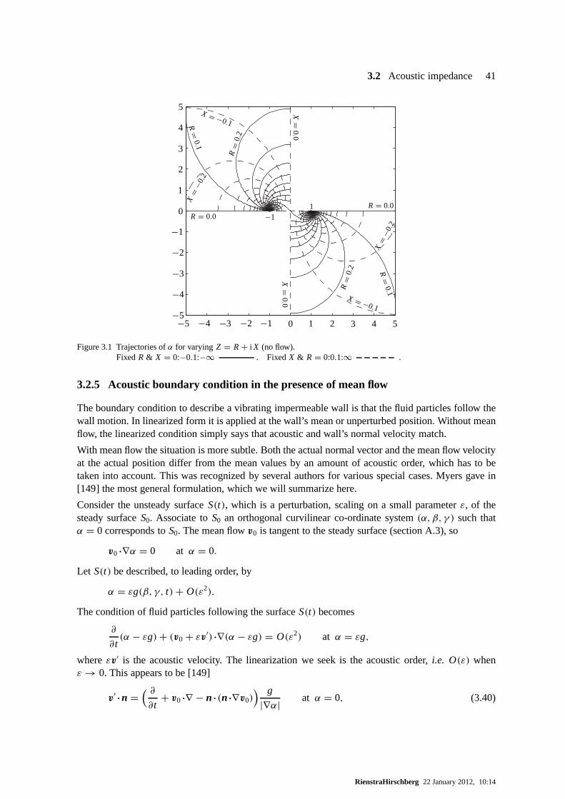
3.2 Acoustic impedance 41
X=
0.0
X=
0.0
X = −0.1
X = −0.1
X=
−0.2
X=
−0.2
R = 0.0
R = 0.0
R=
0.1
R=
0.1
R=
0.2
R=
0.2
1−1
5
5
4
4
3
3
2
2
1
1
0
0
−1
−1
−2
−2
−3
−3
−4
−4−5−5
Figure 3.1 Trajectories ofα for varying Z = R + i X (no flow).Fixed R & X = 0:−0.1:−∞ . FixedX & R = 0:0.1:∞ .
3.2.5 Acoustic boundary condition in the presence of mean flow
The boundary condition to describe a vibrating impermeablewall is that the fluid particles follow thewall motion. In linearized form it is applied at the wall’s mean or unperturbed position. Without meanflow, the linearized condition simply says that acoustic andwall’s normal velocity match.
With mean flow the situation is more subtle. Both the actual normal vector and the mean flow velocityat the actual position differ from the mean values by an amount of acoustic order, which has to betaken into account. This was recognized by several authors for various special cases. Myers gave in[149] the most general formulation, which we will summarizehere.
Consider the unsteady surfaceS(t), which is a perturbation, scaling on a small parameterε, of thesteady surfaceS0. Associate toS0 an orthogonal curvilinear co-ordinate system(α, β, γ ) such thatα = 0 corresponds toS0. The mean flowv0 is tangent to the steady surface (section A.3), so
v0·∇α = 0 at α = 0.
Let S(t) be described, to leading order, by
α = εg(β, γ, t)+ O(ε2).
The condition of fluid particles following the surfaceS(t) becomes
∂
∂t(α − εg)+ (v0 + εv′)·∇(α − εg) = O(ε2) at α = εg,
whereεv′ is the acoustic velocity. The linearization we seek is the acoustic order,i.e. O(ε) whenε → 0. This appears to be [149]
v′ ·n =( ∂∂t
+ v0·∇ − n·(n·∇v0)) g
|∇α| at α = 0, (3.40)
RienstraHirschberg 22 January 2012, 10:14
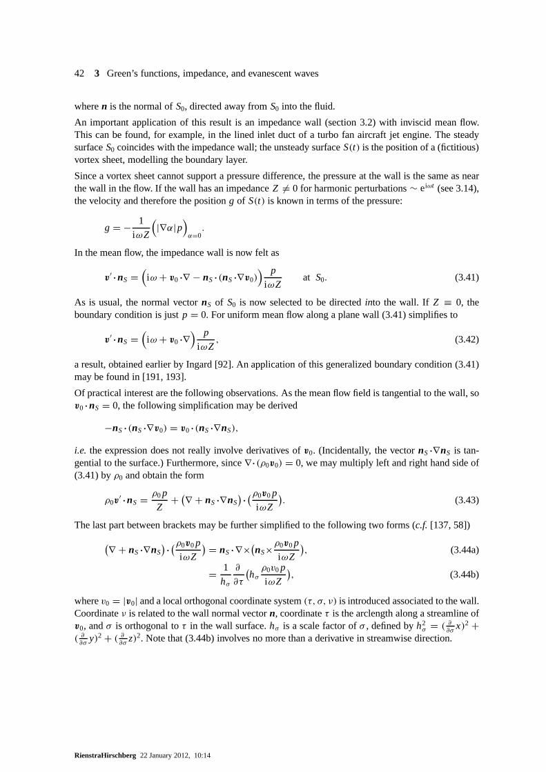
42 3 Green’s functions, impedance, and evanescent waves
wheren is the normal ofS0, directed away fromS0 into the fluid.
An important application of this result is an impedance wall(section 3.2) with inviscid mean flow.This can be found, for example, in the lined inlet duct of a turbo fan aircraft jet engine. The steadysurfaceS0 coincides with the impedance wall; the unsteady surfaceS(t) is the position of a (fictitious)vortex sheet, modelling the boundary layer.
Since a vortex sheet cannot support a pressure difference, the pressure at the wall is the same as nearthe wall in the flow. If the wall has an impedanceZ 6= 0 for harmonic perturbations∼ eiωt (see 3.14),the velocity and therefore the positiong of S(t) is known in terms of the pressure:
g = − 1
iωZ
(|∇α|p
)α=0.
In the mean flow, the impedance wall is now felt as
v′ ·nS =(iω + v0·∇ − nS·(nS·∇v0)
) p
iωZat S0. (3.41)
As is usual, the normal vectornS of S0 is now selected to be directedinto the wall. If Z ≡ 0, theboundary condition is justp = 0. For uniform mean flow along a plane wall (3.41) simplifies to
v′ ·nS =(iω + v0·∇
) p
iωZ, (3.42)
a result, obtained earlier by Ingard [92]. An application ofthis generalized boundary condition (3.41)may be found in [191, 193].
Of practical interest are the following observations. As the mean flow field is tangential to the wall, sov0·nS = 0, the following simplification may be derived
−nS·(nS·∇v0) = v0·(nS·∇nS),
i.e. the expression does not really involve derivatives ofv0. (Incidentally, the vectornS·∇nS is tan-gential to the surface.) Furthermore, since∇·(ρ0v0) = 0, we may multiply left and right hand side of(3.41) byρ0 and obtain the form
ρ0v′ ·nS = ρ0p
Z+
(∇ + nS·∇nS
)·(ρ0v0 p
iωZ
). (3.43)
The last part between brackets may be further simplified to the following two forms (c.f. [137, 58])
(∇ + nS·∇nS
)·(ρ0v0p
iωZ
)= nS·∇×
(nS×
ρ0v0p
iωZ
), (3.44a)
= 1
hσ
∂
∂τ
(hσρ0v0 p
iωZ
), (3.44b)
wherev0 = |v0| and a local orthogonal coordinate system(τ, σ, ν) is introduced associated to the wall.Coordinateν is related to the wall normal vectorn, coordinateτ is the arclength along a streamline ofv0, andσ is orthogonal toτ in the wall surface.hσ is a scale factor ofσ , defined byh2
σ = ( ∂∂σ
x)2 +( ∂∂σ
y)2 + ( ∂∂σ
z)2. Note that (3.44b) involves no more than a derivative in streamwise direction.
RienstraHirschberg 22 January 2012, 10:14
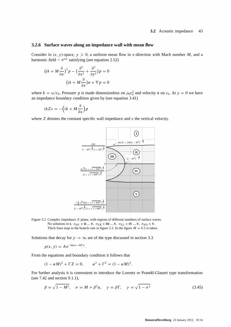
3.2 Acoustic impedance 43
3.2.6 Surface waves along an impedance wall with mean flow
Consider in(x, y)-space,y > 0, a uniform mean flow inx-direction with Mach numberM, and aharmonic field∼ eiωt satisfying (see equation 2.52)
(i k + M
∂
∂x
)2p −
( ∂2
∂x2+ ∂2
∂y2
)p = 0
(i k + M
∂
∂x
)v + ∇ p = 0
wherek = ω/c0. Pressurep is made dimensionless onρ0c20 and velocityv on c0. At y = 0 we have
an impedance boundary condition given by (see equation 3.41)
i k Zv = −(i k + M
∂
∂x
)p
whereZ denotes the constant specific wall impedance andv the vertical velocity.
2M i
(1 − M2)32 (1 + M2)
12
0
4√
2(1 +
√1 + 8M2 ) 1
2
(3 +
√1 + 8M2 ) 3
2
−i 12
√2 M
(3 +
√1 + 8M2 ) 3
2
(1 − M2) 3
2(1 +
√1 + 8M2 ) 1
2
(1 − M2)− 3
2
Im(Z) = 2M(1 − M2)− 3
2
I
IIIII
IV
V
Figure 3.2 Complex impedanceZ-plane, with regions of different numbers of surface waves.No solutions inI , σH I ∈ II . . . V , σS R∈ III . . . V , σSL ∈ IV . . . V , σH S ∈ V.Thick lines map to the branch cuts in figure 3.3. In the figureM = 0.5 is taken.
Solutions that decay fory → ∞ are of the type discussed in section 3.3
p(x, y) = Ae−ikαx−ik0y .
From the equations and boundary condition it follows that
(1 − αM)2 + 0Z = 0, α2 + 02 = (1 − αM)2.
For further analysis it is convenient to introduce the Lorentz or Prandtl-Glauert type transformation(see 7.42 and section 9.1.1),
β =√
1 − M2, σ = M + β2α, γ = β0, γ =√
1 − σ 2 (3.45)
RienstraHirschberg 22 January 2012, 10:14
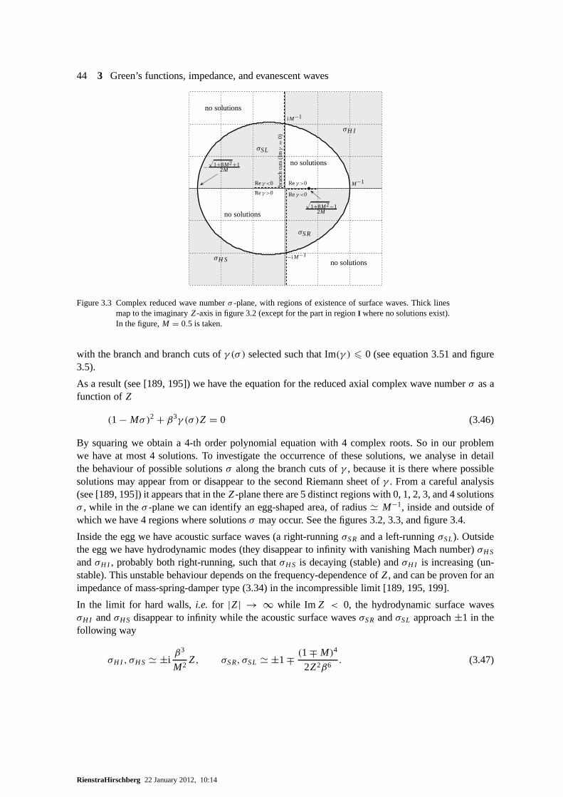
44 3 Green’s functions, impedance, and evanescent waves
i M−1
−i M−1
M−1
−√
1+8M2+12M
√1+8M2−1
2M
σSL
σH I
σH S
σSR
no solutions
no solutions
no solutions
no solutions
bra
nch
cuts
(Imγ
=0
)
Reγ>0
Reγ<0
Reγ<0
Reγ>0
Figure 3.3 Complex reduced wave numberσ -plane, with regions of existence of surface waves. Thick linesmap to the imaginaryZ-axis in figure 3.2 (except for the part in regionI where no solutions exist).In the figure,M = 0.5 is taken.
with the branch and branch cuts ofγ (σ ) selected such that Im(γ ) 6 0 (see equation 3.51 and figure3.5).
As a result (see [189, 195]) we have the equation for the reduced axial complex wave numberσ as afunction of Z
(1 − Mσ )2 + β3γ (σ )Z = 0 (3.46)
By squaring we obtain a 4-th order polynomial equation with 4complex roots. So in our problemwe have at most 4 solutions. To investigate the occurrence ofthese solutions, we analyse in detailthe behaviour of possible solutionsσ along the branch cuts ofγ , because it is there where possiblesolutions may appear from or disappear to the second Riemannsheet ofγ . From a careful analysis(see [189, 195]) it appears that in theZ-plane there are 5 distinct regions with 0, 1, 2, 3, and 4 solutionsσ , while in theσ -plane we can identify an egg-shaped area, of radius' M−1, inside and outside ofwhich we have 4 regions where solutionsσ may occur. See the figures 3.2, 3.3, and figure 3.4.
Inside the egg we have acoustic surface waves (a right-running σS R and a left-runningσSL). Outsidethe egg we have hydrodynamic modes (they disappear to infinity with vanishing Mach number)σH S
andσH I , probably both right-running, such thatσH S is decaying (stable) andσH I is increasing (un-stable). This unstable behaviour depends on the frequency-dependence ofZ, and can be proven for animpedance of mass-spring-damper type (3.34) in the incompressible limit [189, 195, 199].
In the limit for hard walls,i.e. for |Z| → ∞ while Im Z < 0, the hydrodynamic surface wavesσH I andσH S disappear to infinity while the acoustic surface wavesσS R andσSL approach±1 in thefollowing way
σH I , σH S ' ±iβ3
M2Z, σS R, σSL ' ±1 ∓ (1 ∓ M)4
2Z2β6. (3.47)
RienstraHirschberg 22 January 2012, 10:14

3.2 Acoustic impedance 45
i
i
1 + i
Z = 0
Z = 1
−0.4i
1 − 0.4i
−i
1 − i
1 − i
−2i
−2i
1 − 2i
1 − 2i
−3i
−3i
1 − 3i
1 − 3i
−3.6i
1 − 3.6i
5
5
4
4
2
2
3
3
1
1
0
0
−1
−1
−2
−2
−3
−3
−4
−4−5−5
Figure 3.4 Trajectories ofσ for varying Z = R + i X andM = 0.5.Fixed R & X = −∞:0.2:∞ . FixedX & R = 0:0.2:∞ .
3.2.7 Instability, ill-posedness, and a regularization
Although the Ingard-Myers limit of a vanishing mean flow boundary layer is very reasonable for afixed frequency, with all pertaining wavelengths being muchlonger than the boundary layer thickness,it is totally useless [22, 20] in time domain [198].
The problem is that if we gradually reduce the boundary layer, one of the above hydrodynamic surfacewaves changes from a convective instability (a positive growth rate for at least part of the wave numberspectrum but always with a group velocity directed downstream) to an absolute instability (positive,0, and negative group velocities yielding unstable behaviour everywhere) [199]. At the same time thegrowth rate increases until it becomes infinite in the Ingard-Myers limit of a vanishing boundary layer.This implies that in time domain, any perturbation excites in zero time an infinitely large instability.A model or mathematical problem with this property is calledill-posed.
The (presumably) convective instability has been observedexperimentally [8], but the absolute insta-bility probably only numerically [31]. The reason appears to be [199] that the critical boundary layerthickness, where the instability of the system changes fromconvective to absolute, is in any practicalsituation so small (several microns) that is has never been realised.
One way to cure this problem of the Ingard-Myers model is to regularise the boundary condition byincluding the effect of a boundary layer of very thin but non-zero thicknessh. For example like in
RienstraHirschberg 22 January 2012, 10:14
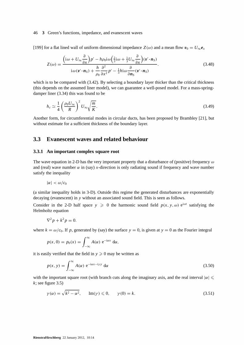
46 3 Green’s functions, impedance, and evanescent waves
[199] for a flat lined wall of uniform dimensional impedanceZ(ω) and a mean flowv0 = U∞ex
Z(ω) =
(iω + U∞
∂
∂x
)p′ − hρ0iω
(23iω + 1
3U∞∂
∂x
)(v′ ·nS)
iω(v′ ·nS)+ h
ρ0
∂2
∂x2p′ − 1
3hiω∂
∂nS(v′ ·nS)
. (3.48)
which is to be compared with (3.42). By selecting a boundary layer thicker than the critical thickness(this depends on the assumed liner model), we can guarantee awell-posed model. For a mass-spring-damper liner (3.34) this was found to be
hc ' 1
4
(ρ0U∞
R
)2
U∞
√m
K. (3.49)
Another form, for circumferential modes in circular ducts,has been proposed by Brambley [21], butwithout estimate for a sufficient thickness of the boundary layer.
3.3 Evanescent waves and related behaviour
3.3.1 An important complex square root
The wave equation in 2-D has the very important property thata disturbance of (positive) frequencyωand (real) wave numberα in (say)x-direction is only radiating sound if frequency and wave numbersatisfy the inequality
|α| < ω/c0
(a similar inequality holds in 3-D). Outside this regime thegenerated disturbances are exponentiallydecaying (evanescent) iny without an associated sound field. This is seen as follows.
Consider in the 2-D half spacey > 0 the harmonic sound fieldp(x, y, ω) eiωt satisfying theHelmholtz equation
∇2 p + k2p = 0.
wherek = ω/c0. If p, generated by (say) the surfacey = 0, is given aty = 0 as the Fourier integral
p(x,0) = p0(x) =∫ ∞
−∞A(α) e−iαx dα,
it is easily verified that the field iny > 0 may be written as
p(x, y) =∫ ∞
−∞A(α) e−iαx−iγ y dα (3.50)
with the important square root (with branch cuts along the imaginary axis, and the real interval|α| 6k; see figure 3.5)
γ (α) =√
k2 − α2, Im(γ ) 6 0, γ (0) = k. (3.51)
RienstraHirschberg 22 January 2012, 10:14
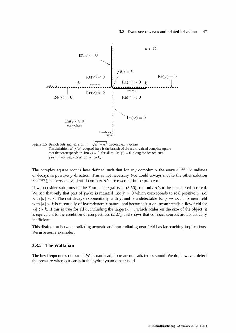
3.3 Evanescent waves and related behaviour 47
real axis
imaginaryaxis
• •
HHHj
QQQk
?6
����
γ (0) = k
k−k
Im(γ ) = 0
Im(γ ) = 0Im(γ ) 6 0
everywhere
Re(γ ) = 0
Re(γ ) = 0Re(γ ) > 0
Re(γ ) > 0Re(γ ) < 0
branch cut
Re(γ ) < 0
branch cut
α ∈ C
Figure 3.5 Branch cuts and signs ofγ =√
k2 − α2 in complex α-plane.The definition ofγ (α) adopted here is the branch of the multi-valued complex squareroot that corresponds to Im(γ ) 6 0 for all α. Im(γ ) = 0 along the branch cuts.γ (α) ' −iα sign(Reα) if |α| � k,
The complex square root is here defined such that for any complex α the wavee−iαx−iγ y radiatesor decays in positivey-direction. This is not necessary (we could always invoke the other solution∼ e+iγ y), but very convenient if complexα’s are essential in the problem.
If we consider solutions of the Fourier-integral type (3.50), the onlyα’s to be considered are real.We see that only that part ofp0(x) is radiated intoy > 0 which corresponds to real positiveγ , i.e.with |α| < k. The rest decays exponentially withy, and is undetectable fory → ∞. This near fieldwith |α| > k is essentially of hydrodynamic nature, and becomes just an incompressible flow field for|α| � k. If this is true for allα, including the largestα−1, which scales on the size of the object, itis equivalent to the condition of compactness (2.27), and shows that compact sources are acousticallyinefficient.
This distinction between radiating acoustic and non-radiating near field has far reaching implications.We give some examples.
3.3.2 The Walkman
The low frequencies of a small Walkman headphone are not radiated as sound. We do, however, detectthe pressure when our ear is in the hydrodynamic near field.
RienstraHirschberg 22 January 2012, 10:14
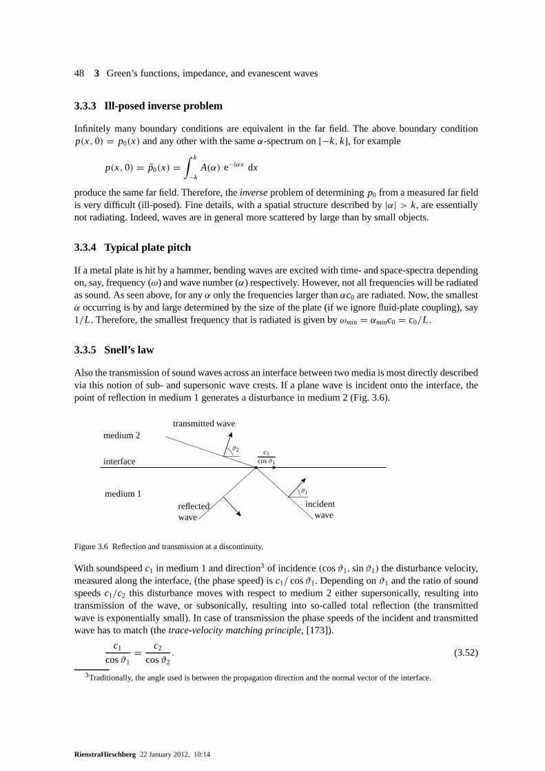
48 3 Green’s functions, impedance, and evanescent waves
3.3.3 Ill-posed inverse problem
Infinitely many boundary conditions are equivalent in the far field. The above boundary conditionp(x,0) = p0(x) and any other with the sameα-spectrum on[−k, k], for example
p(x,0) = p0(x) =∫ k
−kA(α) e−iαx dx
produce the same far field. Therefore, theinverseproblem of determiningp0 from a measured far fieldis very difficult (ill-posed). Fine details, with a spatial structure described by|α| > k, are essentiallynot radiating. Indeed, waves are in general more scattered by large than by small objects.
3.3.4 Typical plate pitch
If a metal plate is hit by a hammer, bending waves are excited with time- and space-spectra dependingon, say, frequency (ω) and wave number (α) respectively. However, not all frequencies will be radiatedas sound. As seen above, for anyα only the frequencies larger thanαc0 are radiated. Now, the smallestα occurring is by and large determined by the size of the plate (if we ignore fluid-plate coupling), say1/L. Therefore, the smallest frequency that is radiated is given byωmin = αminc0 = c0/L.
3.3.5 Snell’s law
Also the transmission of sound waves across an interface between two media is most directly describedvia this notion of sub- and supersonic wave crests. If a planewave is incident onto the interface, thepoint of reflection in medium 1 generates a disturbance in medium 2 (Fig. 3.6).
ϑ1
ϑ2 c1
cosϑ1
reflectedwave
incidentwave
transmitted wave
medium 1
medium 2
interface
Figure 3.6 Reflection and transmission at a discontinuity.
With soundspeedc1 in medium 1 and direction3 of incidence(cosϑ1, sinϑ1) the disturbance velocity,measured along the interface, (the phase speed) isc1/ cosϑ1. Depending onϑ1 and the ratio of soundspeedsc1/c2 this disturbance moves with respect to medium 2 either supersonically, resulting intotransmission of the wave, or subsonically, resulting into so-called total reflection (the transmittedwave is exponentially small). In case of transmission the phase speeds of the incident and transmittedwave has to match (thetrace-velocity matching principle, [173]).
c1
cosϑ1= c2
cosϑ2. (3.52)
3Traditionally, the angle used is between the propagation direction and the normal vector of the interface.
RienstraHirschberg 22 January 2012, 10:14
3.3 Evanescent waves and related behaviour 49
This is equivalent to Snell’s law ([52, 173]), from which we can determine the angleθ2 of the trans-mitted wave with the interface.
For the amplitudes (the reflection and transmission coefficients) we have to do a bit more. See forexample the next problem.
Snellius along an air-bulk interface
If the interface is between air and a dissipative bulk absorber, covered with a top plate, the idea is thesame, but we need a more precise calculation.
Suppose we have in the airy < 0
iωρ− + ρ0∇·v− = 0,
iωρ0v− + ∇ p− = 0,
p− = c20ρ−,
(3.53)
while the bulkabsorber iny > 0 is described by the model
iω�ρ+ + ρ0∇·v+ = 0,
(iωρe + σ )v+ + ∇ p+ = 0,
p+ = c2eρ+.
(3.54)
At the interfacey = 0 we have a pressure jump due to the top plate and continuity ofmass
p−(x,0) − p+(x,0) = − Z
iωρ0
∂
∂yp−(x,0),
∂
∂yp−(x,0) = ζ
∂
∂yp+(x,0), ζ = ρ0
ρe − iσ/ω.
(3.55)
Eliminatev to get
∇2 p + k2 p = 0, k = ω
c0, y < 0
∇2 p + µ2 p = 0, µ = ω
ce
√�
ζ, y > 0
(3.56)
Assume incident a plane wave of unit amplitude iny < 0, propagation in(cosφ, sinφ)-direction, anda reflected wave, together given by
p−(x, y) = e−ikx cosφ−ikysinφ +Re−ikx cosφ+iky sinφ (3.57)
Assume the following transmitted wave iny > 0, which is caused by the incident wave and thereforehas the samex-dependence (the trace-velocity matching principle)
p+(x, y) = f (y)e−ikx cosφ (3.58)
From the equation forp+ it follows that f (y) = T e−iγ y with γ 2 = µ2 − k2 cos2φ. Since thetransmitted wave is decaying fory → ∞, we choose the branch of the square root with Im(γ ) 6 0.
p+(x, y) = T e−ikx cosφ−iγ y, γ =√µ2 − k2 cos2 φ, Im γ 6 0. (3.59)
RienstraHirschberg 22 January 2012, 10:14
50 3 Green’s functions, impedance, and evanescent waves
The direction of the transmitted wave is thus
(k cosφ,Reγ )√k2 cos2 φ + (Reγ )2
. (3.60)
From the interface conditions we have
(1 + R)e−ikx cosφ −T e−ikx cosφ = (Z/ρ0c0)(1 − R) sinφ e−ikx cosφ
−i k(1 − R) sinφ e−ikx cosφ = −i ζγ T e−ikx cosφ
with solution
R =
Z
ρ0c0+ k
ζγ− 1
sinφZ
ρ0c0+ k
ζγ+ 1
sinφ
, T =2
k
ζγ
Z
ρ0c0+ k
ζγ+ 1
sinφ
(3.61)
This solution includes the previous problem of a simple change in sound speedc0.
3.3.6 Silent vorticity
The field of a moving point source may be entirely acoustical,with essentially no other than convec-tion effects. It is, however, possible, and physically indeed usual, that a fluctuating moving line forcegenerates a surface or sheet of trailing vorticity. This vorticity is generated in addition of the acousticfield and is itself also of acoustic order, but, apart from some coupling effects, silent. Typical examplesare (the trailing edge of) a fluctuating wing, a propeller blade, or a flag pole in the wind. The amountof generated vorticity is not a priori known but depends on details of the vortex shedding process (e.g.described by the Kutta condition), usually not included in an acoustic model. Indeed, this vorticitysolution comes into the problem as an eigensolution as soon as continuity of the potential along meanflow streamlines is released as condition. A potential discontinuity corresponds to a vortex sheet.
Although convected vorticity is silent (it exists without pressure fluctuations) its presence may stillbe acoustically important. Near a solid surface (typicallythe surface from which the vorticity is shed)the velocity corresponding to the free vorticity cannot exist, as the field has to satisfy the vanishingnormal velocity condition. This induces a fluctuating pressure along the surface which radiates out assound, apparently from the surface but of course really the vorticity is the source. Examples are thewhistling sound produced by a thin pipe or wire in the wind (aeolian sound), and the trailing edgenoise – as far as it is due to shed-vorticity – from a blunt-edged airfoil. See for example [186].
We will not consider the generation process here in detail, but only indicate the presence of the eigen-solution for a distinct source far upstream.
Consider in a 2D medium a uniform mean flow(U,0) with velocity perturbations∇ϕ and pressureperturbationsp small enough for linearization. Bernoulli’s equation and the mass conservation equa-tion become then
ρ0∂ϕ
∂t+ ρ0U
∂ϕ
∂x+ p = 0, (3.62a)
∂p
∂t+ U
∂p
∂x+ ρ0c
20∇2ϕ = 0, (3.62b)
ϕ → 0 for |y| → ∞. (3.62c)
RienstraHirschberg 22 January 2012, 10:14
3.3 Evanescent waves and related behaviour 51
This may be combined to a wave equation, although the hydrodynamic field is more easily recognizedin the present form4. Possible eigensolutions (solutions without source) for the free field problem (nosolid objects) are given by
p(x, y, t) = 0 (3.63a)
ϕ(x, y, t) = f (x − Ut, y) (3.63b)
∇2 f (x, y) = 0. (3.63c)
for suitable functionsf (x, y). A non-trivial solution f decaying both fory → ∞ and y → −∞is not possible if f is continuous, but if we allowf to be discontinuous along, say,y = 0 (anysurface parallel to the mean flow is possible), of course under the additional conditions aty = 0of a continuous pressurep and continuous vertical velocity∂ϕ/∂y, then we may find with Fouriertransformation
ϕ(x, t) =∫ ∞
−∞F(α) sign(y)e−α|y|−iα(x−Ut) dα. (3.64)
This discontinuity relates to a concentrated layer of vorticity (vortex sheet), and is a typical (hydrody-namic) phenomenon of acoustics with mean flow. The shedding of vorticity (on the scale of the linearacoustics) would not occur without mean flow.
For a harmonic force (for example, a Von Kármán vortex streetmodelled by an undulating vortexsheet) with frequencyω we have only one wave numberα = ω/U in the problem:
ϕ(x, t) = F0 sign(y)exp(iωt − i
ω
Ux − ω
U|y|
). (3.65)
This important parameterω/U is called the “hydrodynamic wave number”. Together with a suitablelength scaleL it yields the dimensionless numberωL/U called “Strouhal number”.
It may be noted that this hydrodynamic field has an averaged intensity, directed inx-direction, equalto (note thatp ≡ 0)
〈I ·ex〉 = 1
2Uρ0
∣∣∣∂ϕ∂x
∣∣∣2
= ω2
U2|F0|2 e−2 ωU |y| .
The total power output in flow direction is then∫ ∞
−∞〈I ·ex〉 dy = ω
U|F0|2. (3.66)
In the case of an acoustic field (for example the field that triggered the vortices associated to thehydrodynamic field) the intensity has a non-zero component in y-direction, and in addition to thepurely hydrodynamic power (3.66) some acoustic energy disappears into, or appears from, the vortexsheety = 0. See section 9.1.3 and [115, 186, 85, 188, 72].
4Equations (3.62a,3.62b) may be combined to the convected wave equation
c20∇2ϕ − (ϕt t + 2Uϕxt + U2ϕxx) = 0
which reduces under the Prandtl-Glauert transformation (see 7.42)ϕ(x, y, t) = ψ(X, y, T) with X = x/β, T = βt +Mx/c0β, M = U/c0, β = √
(1 − M2) to the ordinary wave equation forψ , and a pressure given byp = −ρ0(ψT +UψX)/β. In this way we may obtain from any no-flow solutionψ a solution to the problem with flow. However, care shouldbe taken.
An integrable singularity in∇ψ , as would occur at a sharp edge, corresponds without flow to a finite pressure. With flowit corresponds to a singular pressure (from theψX-term). If this is physically unacceptable, for example if the edge is atrailing edge and the sound field induces the shedding of vorticity, a Kutta condition of finite pressure is required and thesolution is to be modified to include the field of the shed vorticity (a discontinuousϕ).
RienstraHirschberg 22 January 2012, 10:14
52 3 Green’s functions, impedance, and evanescent waves
Exercises
a) Consider the sound produced by thunder, modelled as an infinite line source, fired impulsively. Explainthe typical long decay after the initial crack.
b) Consider in (x, y, z)-space the planez = 0, covered uniformly with point sources which are all firedinstantaneously att = τ :δ(t −τ )δ(x−x0)δ(y− y0)δ(z) (z0 = 0). Calculate the sound field at some distance away from the plane.
c) Consider an infinite equidistant row of harmonically oscillating line sources∑n δ(x − nd)δ(y) eiωt , placed in thex, z-plane a distanced from each other. Show that constructive
interference in the far field will only occur in directions with an angleθ such that
kdcosθ = 2πm; m = 0,1,2, . . .
wherek = ω/c0.
d) The same question for a row of alternating line sources.
e) What is the dimension ofδ(x) if x denotes a physical coordinate with dimension “length”?
f) Prove the identities (C.36a) and (C.36b).
g) Consider a finite volumeV with surfaceS and outward surface normaln. On V is defined a smoothvector fieldv. Prove, by using surface distributions, Gauss’ theorem∫
V∇·v dx =
∫
Sv ·n dσ.
h) Work out the expression (3.36) for the reflected waveg in the case of formula (3.38) withm = 0.
i) We define an ideal open end as a position at whichp = 0 in a tube. Calculate reflection coefficientRand impedanceZ for such an open end.
j) The same question for an ideal closed end defined byv = 0.
k) Given a uniform duct betweenx = −∞ andx = 0, with impedanceZ0 of the planex = 0 seen fromthex < 0 side. CalculateZL , the impedance of the planex = −L, seen fromx < 0.
l) Prove causality of the impedanceZ(ω) = R+ iωm − i K/ω. Find the inverse Fourier transform of bothZ andY = 1/Z.
m) Determine the reflection coefficientR of a harmonic plane wave
p(x) = e−ik·x +Re−i k·x, v(x) = kρ0�
e−ik·x +Rkρ0�
e−i k·x
with k = k(cosϑ, sinϑ), k = k(cosϑ,− sinϑ), k = ‖k‖, c0k = �, � = ω − u0k cosϑ , incident fromy < 0 in a mean flowv0 = (u0,0) against a wall aty = 0 with impedanceZ. What is the impedancewith R = 0?
RienstraHirschberg 22 January 2012, 10:14
4 One dimensional acoustics
4.1 Plane waves
Plane waves are waves in which the acoustic field only dependson the spatial coordinate (say:x) inthe direction of propagation:p(x, t), ρ(x, t), v(x, t), ... . Such waves may emerge, for example, asapproximations for spheric waves at large distance from a point source, or as waves propagating at afrequency lower than a critical frequencyfc called the cut-off frequency in a hard-walled pipe. As wewill see from the discussion in section 6.4 and section 7.2 the cut-off frequencyfc is of the order ofc0/2d whered is the pipe width (or diameter). The exact value offc depends on the shape of the pipecross section.
If we can neglect friction, then below the cut-off frequency, the (propagating part of the) acoustic fieldin a pipe consists only of plane waves. The condition for the validity of a frictionless approximationyields a lower bound for the frequency we can consider. At high frequencies, the effect of viscosity isconfined to boundary layers of thicknessδA = (2ν/ω)1/2 (whereν = η/ρ is the kinematic viscosity ofthe fluid) near the walls. In order to make a plane wave approximation reasonable we should have thinviscous boundary layers:δA/d � 1. Hence the frequency range in which a plane wave approximationis valid in a pipe is given by:
2ν
πd2� f <
c0
2d.
For air ν = 1.5 × 10⁻⁵ m2/s while for water a typical value isν = 10−6 m2/s. Hence we see thata plane wave approximation will in air be valid over the threedecades of the audio range for a pipewith a diameterd = O(10−2 m). (Check what happens for larger pipes.) This implies thatsuch anapproximation should be interesting when studying pulsations in pipe systems, musical acoustics,speech production, etc.
We therefore focus our attention in this chapter onthe one-dimensional approximation of duct acous-tics. For simplicity we will also assume that any mean flowu0 = u0(x) is also one dimensional. Wewill consider simple models for the boundary conditions. Wewill assume that the side walls are rigid.This implies that there is no transmission of sound through these walls. This is a drastic assumptionwhich excludes any application of our theory to the prediction of environmental noise induced bypipe flows. In such cases the transmission of the sound from the internal flow to the environment is acrucial factor. A large amplitude in the pipe may be harmlessif the acoustic energy stays inside thepipe! Extensive treatment of this transmission problem is given by Norton [158] and Reethof [184].In general the transmission of sound through elastic structures is described in detail by Cremer andHeckl [36], and Junger and Feit [100]. We further ignore thiscrucial problem.
In principle the approximation we will use is limited to pipes with uniform cross sectionsA or, as wewill see in section 8.4, to pipes with slowly varying cross sections (dA/dx �
√A � λ). The most
interesting applications of our approximation will concern sound generated in compact regions as aresult of sudden changes in cross section or localized fluid injection. As we consider low frequencies
54 4 One dimensional acoustics
( f < c0/2d) a region with a length of the order of the pipe widthd will be by definition compact.We will treat these regions separately, taking possible three dimensional effects into account. The(inner-) solution in the compact region is approximated by that of an incompressible flow or a regionof uniform pressure1.
The boundary conditions for this compact region are relatedto the plane wave regions by means ofintegral conservation laws (Appendix A). In this way we willconsider a large variety of phenomena(temperature discontinuities, jumps in cross sections, multiple junctions, air bubbles, turbulence...).In the present chapter we will assume an infinitely long or semi-infinite pipe. This is a pipe whichis so long that as a result of friction the waves travelling towards the pipe end do not induce signif-icant reflections. This will in fact exclude the accumulation of acoustic energy and phenomena likeresonance. This effect is discussed in the next chapter.
A consequence of this assumption is that the acoustic field will not have a large amplitude and thatwe can usually neglect the influence of the acoustic field on a source. The flow is calculated locallywith our previously discussed compact region approximation ignoring any acoustical feedback. Thisexcludes fascinating effects such as whistling. These effects will be discussed in chapter 5.
If the end of the pipe is part of the problem, we will include this end by a linear boundary condition ofimpedance type. The acoustic impedance is a general linear relation in the frequency domain betweenvelocity and pressure,i.e. a convolution product in the time domain (section 3.2). Since pressurecannot depend on the future of the velocity (orvice versa) the discussion of such a linear boundarycondition involves the concept of causality (section 3.2).
We will show how the Green’s function formalism can be used toobtain information on aero-acoustic sound generation by turbulence and to estimate thescattering of sound by a temperaturenon-uniformity. These problems will be reconsidered laterfor free field conditions in chapter 6. It willthen be interesting to see how strong the effect of the confinement is by a comparison of the resultsobtained in this chapter and chapter 5 with those obtained inchapter 6.
Convective effects on the wave propagation will be discussed in chapter 9. We restrict ourselves nowto very low mean flow Mach numbers outside the source regions.
4.2 Basic equations and method of characteristics
4.2.1 The wave equation
We consider a one-dimensional flow in a pipe with uniform cross section. If we neglect friction theconservation laws of mass and momentum are for a one dimensional flow given by:
∂ρ
∂t+ u
∂ρ
∂x+ ρ
∂u
∂x= ∂(ρβ)
∂t(4.1a)
ρ(∂u
∂t+ u
∂u
∂x
)+ ∂p
∂x= fx (4.1b)
whereρβ corresponds to an external mass injection in the flow andfx is an external force per unitvolume.
1For example, the air density fluctuations in an oscillating acoustically compact air bubble in water cannot be neglected,but we can assume that they are uniform within the bubble.
RienstraHirschberg 22 January 2012, 10:14

4.2 Basic equations and method of characteristics 55
We assume now that the field consists of a uniform state (ρ0, p0,u0), plus a perturbation (ρ ′, p′,u′)small enough to allow linearization:
ρ = ρ0 + ρ,′ (4.2a)
p = p0 + p′, (4.2b)
u = u0 + u′. (4.2c)
∂β/∂t and fx, being the cause of the perturbation, must therefore by definition be small. We substitute(4.2a–4.2c) in (4.1a) and (4.1b). Neglecting second and higher order terms we obtain the linearizedequations:
∂ρ ′
∂t+ u0
∂ρ ′
∂x+ ρ0
∂u′
∂x= ρ0
∂β
∂t(4.3a)
ρ0∂u′
∂t+ ρ0u0
∂u′
∂x+ ∂p′
∂x= fx (4.3b)
We can eliminateρ ′ by using the constitutive equation:
p′ = c20ρ
′ (4.4)
which implies that we assume a homentropic flow.
A one-dimensional wave equation is obtained by subtractingthe divergence of the momentum con-servation law (4.3b) from the convected time derivative(∂t + u0∂x) of mass conservation law (4.3a)(to eliminateu′):
( ∂∂t
+ u0∂
∂x
)2p′ − c2
0∂2 p′
∂x2= c2
0
(ρ0∂2β
∂t2− ∂ fx
∂x
). (4.5)
4.2.2 Characteristics
As an alternative we now show the wave equation in characteristic form. This allows a simple geo-metrical interpretation of the solution of initial condition and boundary condition problems with thehelp of a so-called(x, t) diagram. In acoustics this procedure is just equivalent with other procedures.However, when considering high amplitude wave propagation(non-linear acoustics or gas dynam-ics) the method of characteristic will still allow an analytical solution to many interesting problems[226, 112, 166]. Also the characteristics play a crucial rôle in numerical solutions as they determineoptimal discretization schemes, and in particular their conditions of stability.
Using the constitutive equation
∂p
∂t+ u
∂p
∂x= c2
(∂ρ∂t
+ u∂ρ
∂x
)
we can write the mass conservation law (4.1a) as:
1
ρc
(∂p
∂t+ u
∂p
∂x
)+ c
∂u
∂x= c
ρ
∂(ρβ)
∂t
RienstraHirschberg 22 January 2012, 10:14
56 4 One dimensional acoustics
by addition, respectively subtraction, of the momentum conservation law (4.1b) divided byρ, we findthe non-linear wave equation in characteristic form:
( ∂∂t
+ (u ± c)∂
∂x
)(u ±
∫dp
ρc
)= fx
ρ± c
ρ
∂(ρβ)
∂t.
In the absence of source terms this simply states that along the characteristicsc± the Riemann invariant0± is conserved:
0+ = u′ +∫
dp
ρc= constant alongc+ =
{(x, t)
∣∣∣ dx
dt= u + c
}(4.6a)
0− = u′ −∫
dp
ρc= constant alongc− =
{(x, t)
∣∣∣ dx
dt= u − c
}(4.6b)
In the presence of source terms we have:
0± − 0±0 =
∫
c±
(ρ0c
20
∂β
∂t± c0 fx
)dt (4.7)
where the integration is along the respective characteristic. For an ideal gas with constant specific heatwe find by using the fact that the flow is isentropic:
∫dp
ρc= 2c
γ − 1.
In linear approximation in the absence of sources we have
0± = u′ ± p′
ρ0c0along the lines defined byc± : dx
dt= u0 ± c0.
4.2.3 Linear behaviour
In the absence of source terms (the homogeneous problem) we can write the linear perturbationp′ asthe sum of two wavesF andG travelling in opposite directions (along thec+ andc− characteristics):
p′ = F (x − (c0 + u0)t)+ G(x + (c0 − u0)t), (4.8a)
u′ = 1
ρ0c0
(F (x − (c0 + u0)t)− G(x + (c0 − u0)t)
). (4.8b)
This solution can be readily verified by substitution into the homogeneous wave equation. The func-tionsF andG are determined by the initial and boundary conditions. As anexample we consider twosimple problems for the particular case of a quiescent fluidu0 = 0.
Let us first consider a semi-infinite pipe closed by a rigid piston moving with a velocityup(t) startingat t = 0 andx = 0. If up/c0 � 1 we can use an acoustic approximation to solve the problem. Usingthe method of characteristics we first observe in a(x, t) diagram (figure 4.1) that there are two regionsfor x > 0:
region I below the linex = c0t
and
region II above the linex = c0t .
RienstraHirschberg 22 January 2012, 10:14
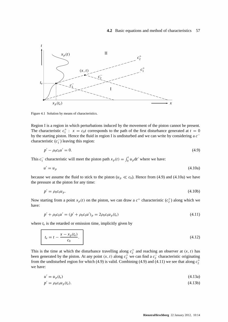
4.2 Basic equations and method of characteristics 57
xp(te)
te
xp(t)
(x, t)
c−1
c−2
c+1
c+2
I
II
x-
t
6
Figure 4.1 Solution by means of characteristics.
Region I is a region in which perturbations induced by the movement of the piston cannot be present.The characteristicc+
1 : x = c0t corresponds to the path of the first disturbance generated att = 0by the starting piston. Hence the fluid in region I is undisturbed and we can write by considering ac−
characteristic (c−1 ) leaving this region:
p′ − ρ0c0u′ = 0. (4.9)
Thisc−1 characteristic will meet the piston pathxp(t) =
∫ t0 updt ′ where we have:
u′ = up (4.10a)
because we assume the fluid to stick to the piston (up � c0). Hence from (4.9) and (4.10a) we havethe pressure at the piston for any time:
p′ = ρ0c0up. (4.10b)
Now starting from a pointxp(t) on the piston, we can draw ac+ characteristic (c+2 ) along which we
have:
p′ + ρ0c0u′ = (p′ + ρ0c0u′)p = 2ρ0c0up(te) (4.11)
wherete is the retarded or emission time, implicitly given by
te = t − x − xp(te)
c0. (4.12)
This is the time at which the disturbance travelling alongc+2 and reaching an observer at(x, t) has
been generated by the piston. At any point(x, t) alongc+2 we can find ac−
2 characteristic originatingfrom the undisturbed region for which (4.9) is valid. Combining (4.9) and (4.11) we see that alongc+
2we have:
u′ = up(te) (4.13a)
p′ = ρ0c0up(te). (4.13b)
RienstraHirschberg 22 January 2012, 10:14
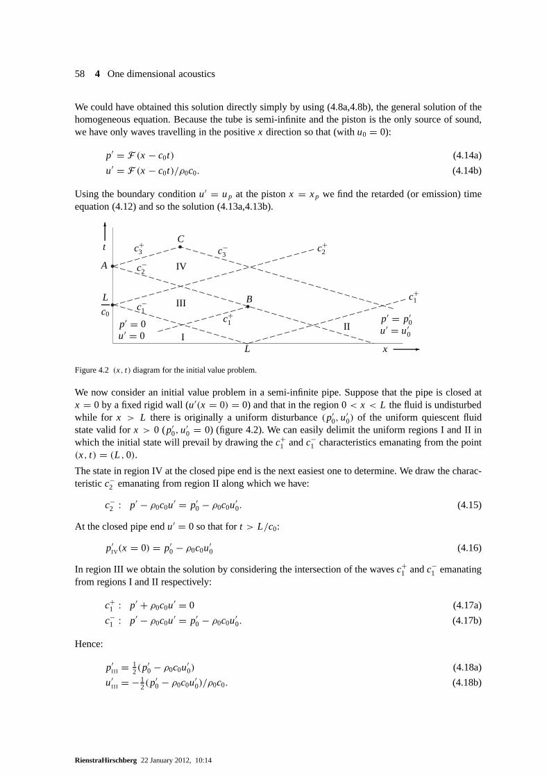
58 4 One dimensional acoustics
We could have obtained this solution directly simply by using (4.8a,4.8b), the general solution of thehomogeneous equation. Because the tube is semi-infinite andthe piston is the only source of sound,we have only waves travelling in the positivex direction so that (withu0 = 0):
p′ = F (x − c0t) (4.14a)
u′ = F (x − c0t)/ρ0c0. (4.14b)
Using the boundary conditionu′ = up at the pistonx = xp we find the retarded (or emission) timeequation (4.12) and so the solution (4.13a,4.13b).
L
c0
A
C
B
t
6
IV
III
c+3 c−
3
c−2
c+2
c−1
Ip′ = 0u′ = 0
L
c+1
c+1
IIp′ = p′
0u′ = u′
0
x -
Figure 4.2 (x, t) diagram for the initial value problem.
We now consider an initial value problem in a semi-infinite pipe. Suppose that the pipe is closed atx = 0 by a fixed rigid wall (u′(x = 0) = 0) and that in the region 0< x < L the fluid is undisturbedwhile for x > L there is originally a uniform disturbance(p′
0,u′0) of the uniform quiescent fluid
state valid forx > 0 (p′0,u
′0 = 0) (figure 4.2). We can easily delimit the uniform regions I and II in
which the initial state will prevail by drawing thec+1 andc−
1 characteristics emanating from the point(x, t) = (L ,0).
The state in region IV at the closed pipe end is the next easiest one to determine. We draw the charac-teristicc−
2 emanating from region II along which we have:
c−2 : p′ − ρ0c0u′ = p′
0 − ρ0c0u′0. (4.15)
At the closed pipe endu′ = 0 so that fort > L/c0:
p′IV(x = 0) = p′
0 − ρ0c0u′0 (4.16)
In region III we obtain the solution by considering the intersection of the wavesc+1 andc−
1 emanatingfrom regions I and II respectively:
c+1 : p′ + ρ0c0u′ = 0 (4.17a)
c−1 : p′ − ρ0c0u′ = p′
0 − ρ0c0u′0. (4.17b)
Hence:
p′III = 1
2(p′0 − ρ0c0u′
0) (4.18a)
u′III = −1
2(p′0 − ρ0c0u′
0)/ρ0c0. (4.18b)
RienstraHirschberg 22 January 2012, 10:14
4.2 Basic equations and method of characteristics 59
Finally for any point in the region IV above the linex = c0(t − L/c0) we have:
c+3 : p′ + ρ0c0u′ = p′
0 − ρ0c0u′0 (4.19a)
c−3 : p′ − ρ0c0u′ = p′
0 − ρ0c0u′0 (4.19b)
so that we have:
u′IV = 0 (4.20a)
p′IV = p′
0 − ρ0c0u′0 (4.20b)
as we already found at the closed pipe end (x = 0). Of course we could have solved this problemwithout an(x, t) diagram, but this requires quite an intellectual effort.
From the previous two examples simple rules are obtained to use an(x, t) diagram in combinationwith the method of characteristics:
a) Indicate on thex andt axis the initial and boundary conditions.
b) Draw the characteristics delimiting the undisturbed regions in which the initial conditions pre-vail.
c) Consider reflection of these boundary characteristics atboundary conditions. (Contact surfacedelimiting regions of different uniform statep0, ρ0, c0, ... will be discussed in section 4.4.) Thisyields a further subdivision of the(x, t) plane in uniform regions.
d) Determine the state at the boundaries at the moment the first message from the initial conditionsarrives.
e) Determine the state in regions where two characteristicsof opposite familiesc+ andc− ema-nating from regions where the solution is known meet.
While for initial value problems the method of characteristics is most efficient, we will use Fourieranalysis when we consider boundary condition problems. Fora steady harmonic perturbation equation(4.8a,4.8b) becomes:
p′ = p+ eiωt−ikx +p− eiωt+ikx (4.21a)
u′ = 1
ρ0c0(p+ eiωt−ikx −p− eiωt+ikx). (4.21b)
wherep± are amplitudes which are functions ofω, andk is the wave number(k = ω/c0).
RienstraHirschberg 22 January 2012, 10:14
60 4 One dimensional acoustics
4.2.4 Non-linear simple waves and shock waves
A general solution of the non-linear one dimensional homentropic flow equations can only be obtainedby numerical methods. In the particular case of a wave propagating into a uniform region the solutionis considerably simplified by the fact that the characteristics emanating from the uniform region allcarry a uniform message. We will show that as a consequence ofthis the other characteristics in thiswave are straight lines in the (x, t)-plane. Such a wave is called a simple wave.
Let us for example consider a wave propagating alongc+-characteristics which meetsc−-waves em-anating from a uniform region. The message carried by thec−-characteristics is:
0− = u −∫
dp
ρc= 0−
0 for all c−. (4.22)
If we now consider ac+-characteristic in the simple wave, we have in addition that0+ is equal toanother constant, specific to that particularc+:
0+ = u +∫
dp
ρc. (4.23)
Addition and subtraction of (4.22) and (4.23) yields, alongthec+, the result
u = 12(0
+ + 0−0 ), (4.24a)∫
dp
ρc= 1
2(0+ − 0−
0 ). (4.24b)
Hence, the velocityu is constant along thec+ considered. As in addition to the thermodynamic quan-tity
∫(dp/ρc) also the entropys is constant along thec+ (because the flow is homentropic), we
conclude that all thermodynamic variables2 are constant along thec+. In particular the speed of soundc =
√(∂p/∂ρ)s is constant along ac+ in the simple wave. Therefore, the slope(u + c) of the c+
characteristic is constant, and the characteristic is a straight line in an(x, t)-diagram.
As an example of an application we consider the simple wave generated forx > 0 by a given boundarycondition p(0, t) at x = 0, assuming a uniform quiescent fluid (u0 = 0) with a speed of soundc = c0
for t < 0. The sound speedc(0, t) at x = 0 is calculated by using the equation of state
p
p0=
( ρρ0
)γ
which implies
c
c0=
( p
p0
) γ−12γ.
The message from thec−-characteristics implies
u = 2c0
γ − 1
( c
c0− 1
)= 2c0
γ − 1
(( p
p0
) γ−12γ − 1
).
We can now easily construct the simple wave by drawing at eachtime t thec+-characteristic emanat-ing from x = 0. We see from these equations that a compression∂
∂t p(0, t) > 0 implies an increase
2For a homogeneous fluid the thermodynamic state is fully determined by two thermodynamic variables.
RienstraHirschberg 22 January 2012, 10:14
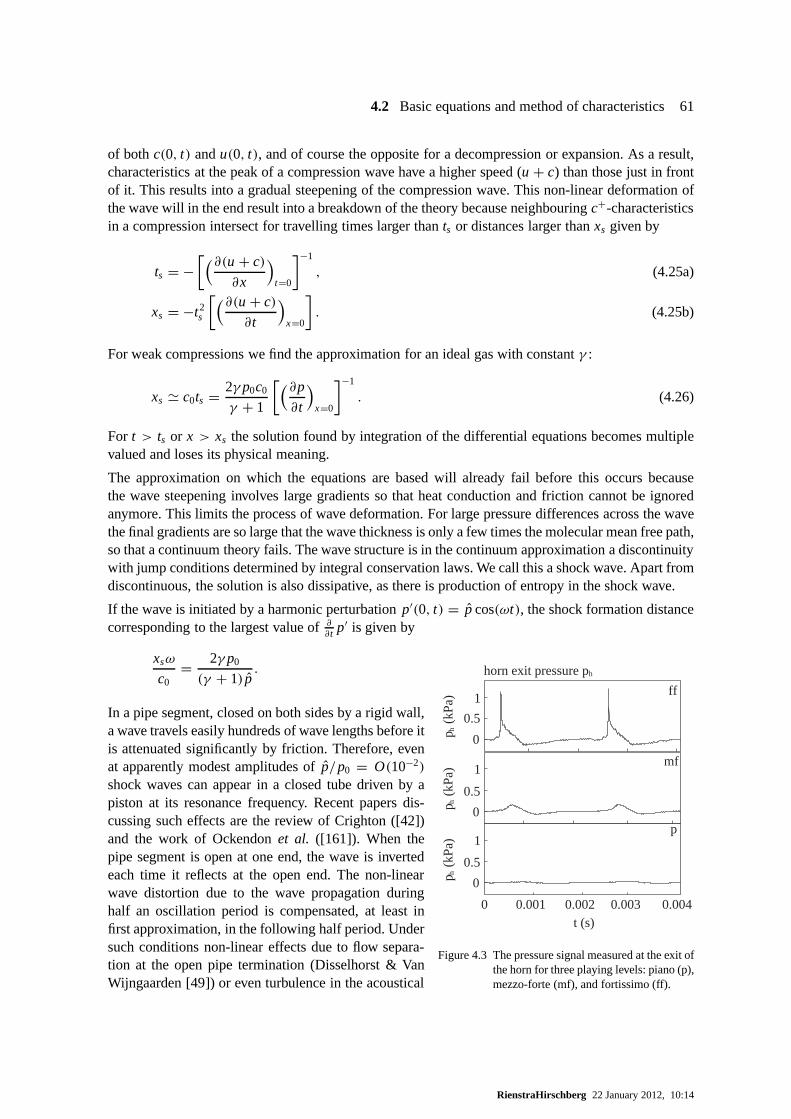
4.2 Basic equations and method of characteristics 61
of bothc(0, t) andu(0, t), and of course the opposite for a decompression or expansion. As a result,characteristics at the peak of a compression wave have a higher speed (u + c) than those just in frontof it. This results into a gradual steepening of the compression wave. This non-linear deformation ofthe wave will in the end result into a breakdown of the theory because neighbouringc+-characteristicsin a compression intersect for travelling times larger thants or distances larger thanxs given by
ts = −[(∂(u + c)
∂x
)t=0
]−1
, (4.25a)
xs = −t2s
[(∂(u + c)
∂t
)x=0
]. (4.25b)
For weak compressions we find the approximation for an ideal gas with constantγ :
xs ' c0ts = 2γ p0c0
γ + 1
[(∂p
∂t
)x=0
]−1
. (4.26)
For t > ts or x > xs the solution found by integration of the differential equations becomes multiplevalued and loses its physical meaning.
The approximation on which the equations are based will already fail before this occurs becausethe wave steepening involves large gradients so that heat conduction and friction cannot be ignoredanymore. This limits the process of wave deformation. For large pressure differences across the wavethe final gradients are so large that the wave thickness is only a few times the molecular mean free path,so that a continuum theory fails. The wave structure is in thecontinuum approximation a discontinuitywith jump conditions determined by integral conservation laws. We call this a shock wave. Apart fromdiscontinuous, the solution is also dissipative, as there is production of entropy in the shock wave.
If the wave is initiated by a harmonic perturbationp′(0, t) = p cos(ωt), the shock formation distancecorresponding to the largest value of∂
∂t p′ is given by
xsω
c0= 2γ p0
(γ + 1) p.
ff
mf
p
horn exit pressure ph
1
0.5
0
1
0.5
0
0.5
1
0p h(k
Pa)
p h(k
Pa)
p h(k
Pa)
t (s)0.001 0.002 0.003 0.0040
Figure 4.3 The pressure signal measured at the exit ofthe horn for three playing levels: piano (p),mezzo-forte (mf), and fortissimo (ff).
In a pipe segment, closed on both sides by a rigid wall,a wave travels easily hundreds of wave lengths before itis attenuated significantly by friction. Therefore, evenat apparently modest amplitudes ofp/p0 = O(10−2)
shock waves can appear in a closed tube driven by apiston at its resonance frequency. Recent papers dis-cussing such effects are the review of Crighton ([42])and the work of Ockendonet al. ([161]). When thepipe segment is open at one end, the wave is invertedeach time it reflects at the open end. The non-linearwave distortion due to the wave propagation duringhalf an oscillation period is compensated, at least infirst approximation, in the following half period. Undersuch conditions non-linear effects due to flow separa-tion at the open pipe termination (Disselhorst & VanWijngaarden [49]) or even turbulence in the acoustical
RienstraHirschberg 22 January 2012, 10:14

62 4 One dimensional acoustics
boundary layer ([133], [235], [3], [55]) can appear before non-linear wave distortion becomes domi-nant.
However, when the pipe is driven by a strongly non-harmonic pressure signalp′(0, t), the wave steep-ening may lead to a shock wave formation before the open end has been reached. This may, forexample, occur in a trombone where the pressure at the exit ofthe horn shows very sharp peaks, asshown in figure (4.3). The increase of the wave distortion with the amplitude explains in such a mu-sical instrument the increase of brightness (the higher harmonics) of the sound with increasing soundlevel (Hirschberg [77]). In open-air loudspeaker horns wave propagate in non-linear way. In mufflersof combustion engines shock waves are also common.
When the non-linear deformation is small, the generation ofthe first harmonicp1 at 2ω0 by a signalp, originally harmonic with frequencyω0, is given by [173]:
p1
p= x
2xs(4.27)
4.3 Source terms
While fx is a source term in (4.1b) which can be realized by non-uniform gravitational or electro-magnetic forces, the source term∂2(ρβ)/∂t2 in (4.1a) does not correspond to the creation of mass(because we consider non-relativistic conditions). Henceif we introduce a source term∂2(ρβ)/∂t2
this term will be a representation of a complex process whichwe include in the 1-D inviscid flowmodel as a source term. For example the effect of fluid injection through a porous side wall in the pipecan be considered by assuming a source term in a uniformly filled pipe with rigid impermeable walls.
In the case offx we may also find useful to summarize the effect of a complex flowsuch as theflow around a ventilation fan by assuming a localized momentum source in a one dimensional model.This is called an actuator disk model. Of course, this kind ofrepresentation of a complex processby a simple source is only possible if we can find a model to calculate this source. This is onlyattractive if a simplified model or an order of magnitude estimate can be used. When the source regionis compact we will be able to find such simple relationships between a simplified local flow modeland the corresponding 1-D sources by applying integral conservation laws over the source regionand neglecting variations in emission time over the source region. The general treatment of the aero-acoustic sources has already been given in section 2.6. We focus here on some additional featureswhich we will use in our applications of the theory.
In a compact region of lengthL and fixed volumeV enclosed by a surfaceS, we will use the conser-vation laws for mass and momentum in integral form (App. A):
d
dt
∫∫∫
V
ρ dx +∫∫
S
ρv ·n dσ = 0 (4.28a)
d
dt
∫∫∫
V
ρv dx +∫∫
S
(P + ρvv)·n dσ =∫∫∫
V
f dx (4.28b)
whereP is the stress tensor (Pi j ).
Within the volumeV we describe the flow here in full three dimensional detail, so(4.28a) has nosource term. However, the source term∂2(ρβ)/∂t2 in the one dimensional representation of the mass
RienstraHirschberg 22 January 2012, 10:14

4.3 Source terms 63
conservation law is supposed to include the effect of the volume integral(d/dt)∫∫∫
ρ dx. In orderto understand this we compare the actual source region with a1-dimensional representation of thissource region (figure 4.4). Integration of (4.1a) over the source region yields for a uniform pipe cross
6?
A
L-�
ϕex
n� n-
SV
1 2
Figure 4.4 One dimensional representation of source region.
section:∫ L
0
∂ρ
∂tdx + (ρu)2 − (ρu)1 =
∫ L
0
∂(ρβ)
∂tdx. (4.29)
If we assumeL to be small compared to the acoustic wave length (compact) and the source term∂2(ρβ)/∂t2 to be uniform we can write in linearized form :
∂β
∂t= 1u′δ(x − y) (4.30)
for a small source region aroundx = y. The value of1u′ = (u′2 − u′
1) to be used in (4.30) is foundby application of (4.28a) to the actual situation. If we assume the flow to be uniform at the planes 1and 2 of cross-sectionA, where it enters and leaves the volumeV , we obtain:
A[(ρu)2 − (ρu)1] = − d
dt
∫∫∫
V
ρ dx + ϕex (4.31)
whereϕex is the externally injected mass flux intoV through the side walls. For identical fluids at bothsides and in linearized approximation for a compact source region we have:
Aρ01u′ = − d
dt
∫∫∫
V
ρ ′ dx + ϕex. (4.32)
Since typical wavelengths are much larger than the compact source region, density and pressure gra-dients are negligible and we can replace the volume integralby the averaged value. We can write fora homentropic flow
1u′ = − V
Aρ0c20
dp′
dt+ ϕex
Aρ0.
In a similar way, if we can neglect the volume contribution(d/dt)∫∫∫
ρv dx to the integral conserva-tion law, we obtain in linear approximation (neglectingρ0u′
22 andρ0u′
12):
fx = 1p′δ(x − y). (4.33)
RienstraHirschberg 22 January 2012, 10:14

64 4 One dimensional acoustics
This source term for the 1-dimensional wave equation can be used as a representation of a complexflow such as that around a ventilation fan.
As an example of a sound source we consider now the effect of the convection of a small fluid particlewith a densityρ and speed of soundc (different fromρ0 andc0) passing through a sudden change inpipe cross section in which we assume a steady isentropic andsubsonic flowu0(x) (figure 4.5). We
123456789012123456789012123456789012123456789012123456789012123456789012123456789012123456789012
A u0(x)
Figure 4.5 Particle convected with the main flowu0(x) through a nozzle.
will first consider the problem by using the linearized form of the integral conservation laws for smalldifferences in density and speed of sound ((ρ − ρ0)/ρ0 � 1 and(c − c0)/c0 � 1). A more formaldiscussion of this effect is given by Morfey in [139].
If the volumeVp of the fluid particle is much smaller than the nozzle volumeV and if the propertiesof the fluid particle do not differ much from that of the rest ofthe fluid, we can assume that the particleis convected with the undisturbed steady flow velocityu0(x). As the particle is small the pressure overthe particle will be uniform and in first approximation equalto the main flow pressurep0(x). p0(x) isgiven by Bernoulli’s equation:
p0(x)+ 12ρ0u
20(x) = constant. (4.34)
The variation in pressurep0(x) will induce a volume variation of the particle, additional to that of themean flow, which is related to the variation in the fluid compressibility
K = 1
ρ
(∂ρ∂p
)S
= 1
ρc2(4.35)
by:
A1u′ = −(K − K0)Vpd
dtp0(xp(t)) (4.36)
which implies a source term:
∂β
∂t= −K − K0
AVp
d
dtp0(xp(t))δ(x − y) (4.37)
where:
up = .x p= u0(xp). (4.38)
because we assume that the particle is convected with the mean flow velocity u0. Furthermore theparticle will exert an additional force on the fluid due to thedensity difference (ρ− ρ0) which impliesa force source term:
fx = 1p′δ(x − y) = −ρ − ρ0
AVp
Dup
Dtδ(x − y) = −ρ − ρ0
AVpu0
du0
dxδ(x − y). (4.39)
RienstraHirschberg 22 January 2012, 10:14

4.4 Reflection at discontinuities 65
This force is due to the difference in inertia between the particle and its environment. Note that for anideal gas the compressibilityK is given by:
K = 1
γ p. (4.40)
Hence for a small particle in this linear approximation the volume source term (4.37) is due to adifference inγ . This term vanishes if we consider the convection of a hot gasparticle (not chemicallydifferent from the environment) which we call an entropy spot. In that case sound production will bedue to the difference of inertia between the entropy spot andthe surrounding fluid. Howe [81] refersto this as acoustical “Bremsstrahlung”.
In a similar way we can describe the effect of a slow variationof the tube cross section areaA onsound waves of low frequency (i.e. d
dx A �√
A � λ). With some care we can derive a suitable one-dimensional approximation, called Webster’s horn equation, to describe the wave propagation (seesection 8.5). To leading order the momentum conservation law is not affected by the cross sectionvariation. The mass conservation law, however, becomes:
∂ρ ′
∂t+ ρ0
A
∂Au′
∂x= 0 (4.41)
This can be interpreted as the linearized continuity equation (4.3a) with a volume source term
∂β
∂t= u′
A
∂A
∂x(4.42)
4.4 Reflection at discontinuities
4.4.1 Jump in characteristic impedanceρc
The procedure described in the previous section to incorporate sources in a compact region into a onedimensional model can also be applied to determine jump conditions over discontinuities in a pipe. Itshould be noted that a mathematically more sound derivation, allowing also higher order corrections,is obtained by using the method of Matched Asymptotic Expansions. This will be worked out in moredetail in chapter 8.
x
ρ1c1 ρ2c2
x=y1 2
Figure 4.6 Jump in acoustic impedance.
We first consider an abrupt change atx = y in speed of soundc and densityρ between two media, 1and 2, in a pipe with uniform cross section (figure 4.6). Considering a thin control volume (betweenthe dotted lines 1 and 2), enclosing the contact surface between the two media and moving with thefluid, we find from the laws of mass and momentum conservation,respectively
1u′ = u′2 − u′
1 = 0, (4.43a)
1p′ = p′2 − p′
1 = 0. (4.43b)
RienstraHirschberg 22 January 2012, 10:14

66 4 One dimensional acoustics
By using the general solution (4.8a,4.8b) of the homogeneous wave equation, we have atx = y forthe jump conditions in the pressure and velocity, respectively:
F1(y − c1t)+ G1(y + c1t) = F2(y − c2t)+ G2(y + c2t), (4.44a)F1(y − c1t)− G1(y + c1t)
ρ1c1= F2(y − c2t)− G2(y + c2t)
ρ2c2. (4.44b)
If, for example, we have a source atx < y generating an incident waveF1, in a tube of infinite lengthso thatG2 = 0, we obtain
G1(x + c1t) = RF1(2y − (x + c1t)
), (4.45a)
F2(x − c2t) = TF1((1 − c1
c2)y + c1
c2(x − c2t)
), (4.45b)
where R = ρ2c2 − ρ1c1
ρ2c2 + ρ1c1, T = 2ρ2c2
ρ2c2 + ρ1c1.
The factorR betweenG1 andF1 is called the reflection coefficient and the factorT betweenF2 andF1
the transmission coefficient. We observe that ifρ1c1 = ρ2c2 the acoustic wave is not reflected at thecontact discontinuity. Inspection of (4.44a,4.44b) forρ1c1 = ρ2c2 also shows that the only solution isF1 = F2 andG1 = G2. This corresponds to results obtained already in section 3.2 when consideringharmonic waves.
4.4.2 Monotonic change in pipe cross section
We now consider a compact transition in pipe cross sectionalarea fromA1 to A2. If the flow is
A1 A2
12
L
Figure 4.7 Abrupt cross sectional area change.
homentropic and there is no flow separation (vorticity is zero) the pressure difference1p′ = p′2 − p′
1across the discontinuity can be calculated by using the incompressible unsteady Bernoulli equation(1.32b):
1p′ = 12ρ0(u
′1
2 − u′2
2)− ρ0∂∂t1ϕ, (4.46)
where1ϕ = ϕ2 − ϕ1 is the potential difference. In linear approximation:
1p′ ' −ρ0∂∂t1ϕ. (4.47)
For a compact smooth change in cross section as in figure (4.7)we have continuity of fluxA1u′1 =
A(x)u′(x), while the potential difference can be estimated as1ϕ =∫ 2
1 u′ dx ' u′1
∫ 21 (A1/A(x))dx ∼
RienstraHirschberg 22 January 2012, 10:14

4.4 Reflection at discontinuities 67
u′1L. The pressure difference1p′ is of the order ofρ0ωu′
1L, which is negligible whenLω/c0 � 1. Wethen have a pressure uniform over the entire region. Note that while this is a very crude approximation,this is a stronger result than just a continuity condition (see section 4.4.4). This condition1p′ = 0can be combined with the linearized mass conservation law inthe low frequency approximation
ρ0A1u′1 = ρ0A2u′
2 (4.48)
to calculate the reflection at a pipe discontinuity.
4.4.3 Orifice and high amplitude behaviour
Instead of a monotonic variation of the pipe areaA we consider an orifice placed in the pipe with anopening areaAd and a thicknessL (figure 4.8). We start with the problem of acoustic wave propagationthrough a stagnant fluid (u0 = 0). In principle, if we use the approximations (4.47) and (4.48) and if we
12345678901234567890123456789011234567890123456789012345678901123456789012345678901234567890112345678901234567890123456789011234567890123456789012345678901123456789012345678901234567890112345678901234567890123456789011234567890123456789012345678901123456789012345678901234567890112345678901234567890123456789011234567890123456789012345678901
12345678901234567890123456789011234567890123456789012345678901123456789012345678901234567890112345678901234567890123456789011234567890123456789012345678901123456789012345678901234567890112345678901234567890123456789011234567890123456789012345678901123456789012345678901234567890112345678901234567890123456789011234567890123456789012345678901
A Ad
L
Figure 4.8 Orifice.
neglect the potential jump1ϕ, we see that the orifice will be completely “transparent” to the acousticwaves. However, ifAd � A we find experimentally a significant effect of such an orifice which isdue to the inertia of the air in the opening. Assuming a uniform velocity and an incompressible flowwithout friction we have from (4.47):
1p′ ' −ρ0A
AdL∂u′
∂t. (4.49)
whereu′ is the acoustic velocity in the pipe. We could also simply have obtained this result by con-sidering the pressure difference1p′ necessary to accelerate the mass of fluid (ρ0Ad L) in the orificeand noticing that the particle velocity in the orifice is given by:
u′d = A
Adu′. (4.50)
In practice (4.49) yields a lower bound for the pressure dropacross the orifice because we neglectedthe inertia of the air in the region outside the orifice. This effect can be taken into account by intro-ducing an “end correction”δ on both sides:
Leff = L + 2δ (4.51)
whereδ appears to be of the order of(Ad/π)1/2. Typically (8/3π)(Ad/π)
1/2 for a circular orifice anda larger value for a slit [91]. This explains why a thin orifice(L → 0) also affects the propagation ofacoustic waves in a pipe. For a circular orifice of radiusa in a thin plate we haveLeff = πa/2 (see[173]).
RienstraHirschberg 22 January 2012, 10:14
68 4 One dimensional acoustics
If we consider a narrow orifice the local velocityu′d in the orifice may become quite large. When the
acoustic particle displacementu′d/ω becomes comparable to the radius of curvature of the edges atthe
entrance and the exit of the orifice non-linear effects and friction will result into acoustically inducedvortex shedding [94, 95, 49, 44]. When the fluid particle displacement becomes comparable to thediameter of the orifice(Ad/π)
1/2u′d/ω = O(1) the vortex shedding can be described in terms of the
formation of a free jet, by assuming that there is no pressuredifference across the boundaries of thejet. The shear layers enclosing the jet are not capable of sustaining a pressure difference. Furthermore,if Ad/A � 1 we assume that the kinetic energy in the flow1
2ρu′d
2 is lost upon deceleration of thejet by turbulent mixing with the air in the pipe. This impliesthat in addition to the linear terms inBernoulli we should add the non-linear effects:
1p′ = −ρ0A
AdL∂u′
∂t− 1
2ρ( A
Adu′
)2. (4.52)
A typical feature of this effect is that the pressure1p′ has now a component12ρu′
d2 which is in phase
with the acoustic velocity, and therefore will involve (acoustic) energy losses that were absent in thesituations discussed until now. These losses are due to the fact that the kinetic energy in the jet isdissipated by turbulence.
The model proposed here appears quite reasonable but in manycases the surface area of the jet issmaller thanAd which implies additional losses[44]. This effect can be as much as a factor 2. The jetcontraction by a factor 2 corresponds to the so called vena contracta at an unflanged pipe entrance.For a thin orifice with sharp edges the jet cross section is a factor π
π+2 narrower than the orifice. Whenthe edges are rounded off the contraction effect disappearsrapidly.
It is interesting to consider now how a mean flow affects the acoustic properties of an orifice. Weassume that the mean flow velocityu0 in the pipe is so small compared to the speed of soundc0
that we can neglect all convective effects on the wave propagation (u0/c0 � 1). As the orifice hasa small aperture(Ad/A), the mean flow velocity in the orifice is significant. We assumea stationaryfrictionless and incompressible flow. The assumption of a frictionless flow fails, however, to describethe flow at the exit of the orifice where as a result of friction the flow separates from the wall and afree jet of surface areaAd is formed.
Assuming further no pressure difference between the jet andits environment we can write for the totalpressure difference1 p0:
1p0 = −12ρ
( A
Adu0
)2. (4.53)
For acoustic velocity fluctuationsu′ we have, neglecting the higher order terms inu′:
1p′ = −ρ0A
AdL∂u′
∂t− ρ0
( A
Ad
)2u0u′. (4.54)
We see from this equation that even in the linear approximation energy is transferred (ρ0(A/Ad)2u0u′2)
from the acoustic field to the flow (where it is dissipated by turbulence). This effect is of course aresult of the forceρ0(ω×v) in Howe’s analogy (section 2.6). The vorticity responsiblefor this islocated in the shear layer that confines the free jet. We will describe the formation of a free jet insection 5.1. The consequence of this effect is that an orificeplaced in a tube with a mean flow is avery efficient damping mechanism. This device is indeed useddownstream of a compressor in orderto avoid the low frequency pulsations that may be induced by the compressor into the pipe system. As
RienstraHirschberg 22 January 2012, 10:14

4.4 Reflection at discontinuities 69
explained by Bechert [10], for any orifice placed at the end ofa pipe one can find a Mach number atwhich the reflection coefficient for long acoustic waves vanishes. Such an orifice acts thus an anechoictermination for low frequencies!
A beautiful property of this damping mechanism is that it is not frequency dependent as long asthe frequency is low enough. This is not the case with the effect of friction and heat transfer whichare strongly frequency dependent (equation 3.13), in a way that at low frequencies friction is quiteinefficient.
u0
u0
a)
b)
Figure 4.9 Vortex shedding at an orifice.
It is interesting, however, to note that under special flow conditions an orifice can produce sound as aresult of vortex shedding. This occurs in particular if the orifice has sharp edges at the entrance wherethe vortices are shed [6] (figure 4.9a) or when the edges are rounded at the downstream side [246, 76](figure 4.9b).
The frequency of the sound produced by the vortex shedding issuch that the period of oscillationroughly corresponds to the travel time of a vortex through the orifice (a Strouhal numberSr =f L/(Au0/Ad) = O(1)). When this sound source couples with a resonator (see next chapter) largeamplitudes may be generated. This is an explanation for human whistling [246, 216]. Flow instabil-ities of this type also occur around pipe arrays such as used in heat exchangers [18]. Whistling cor-responds to self-sustained flow instabilities. In the case of an externally imposed acoustic wave, theperiodic vortex shedding is a non-linear phenomenon which will generate higher harmonics. Hence,suppressing low frequency-pulsations (being mechanically dangerous) with an orifice may be paid bythe generation of high frequency noise which is an environmental problem.
A generalization of the procedure which we introduced intuitively for the orifice can be obtained foran arbitrary compact discontinuity in a pipe system. The acoustical effect of this discontinuity can
RienstraHirschberg 22 January 2012, 10:14
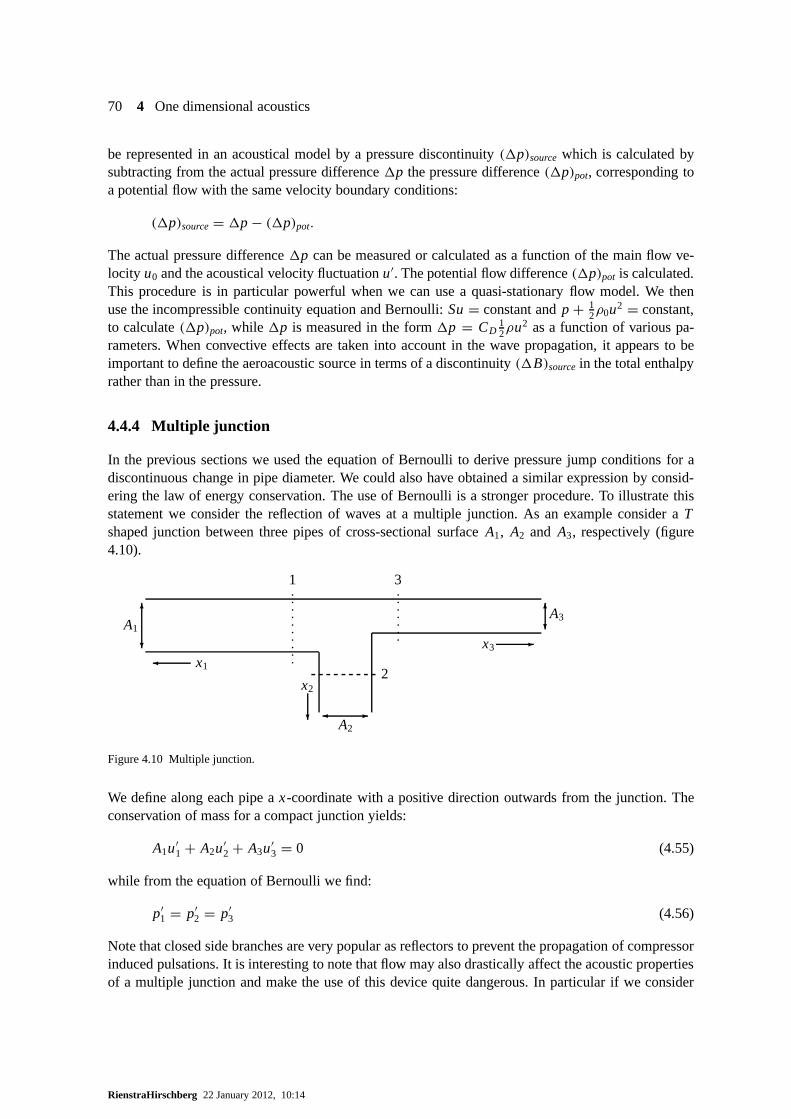
70 4 One dimensional acoustics
be represented in an acoustical model by a pressure discontinuity (1p)source which is calculated bysubtracting from the actual pressure difference1p the pressure difference(1p)pot, corresponding toa potential flow with the same velocity boundary conditions:
(1p)source= 1p − (1p)pot.
The actual pressure difference1p can be measured or calculated as a function of the main flow ve-locity u0 and the acoustical velocity fluctuationu′. The potential flow difference(1p)pot is calculated.This procedure is in particular powerful when we can use a quasi-stationary flow model. We thenuse the incompressible continuity equation and Bernoulli:Su= constant andp + 1
2ρ0u2 = constant,to calculate(1p)pot, while1p is measured in the form1p = CD
12ρu2 as a function of various pa-
rameters. When convective effects are taken into account inthe wave propagation, it appears to beimportant to define the aeroacoustic source in terms of a discontinuity (1B)sourcein the total enthalpyrather than in the pressure.
4.4.4 Multiple junction
In the previous sections we used the equation of Bernoulli toderive pressure jump conditions for adiscontinuous change in pipe diameter. We could also have obtained a similar expression by consid-ering the law of energy conservation. The use of Bernoulli isa stronger procedure. To illustrate thisstatement we consider the reflection of waves at a multiple junction. As an example consider aTshaped junction between three pipes of cross-sectional surface A1, A2 and A3, respectively (figure4.10).
?
6A1 ?
6A3
-�A2
1 3
2� x1
-x3
?
x2
Figure 4.10 Multiple junction.
We define along each pipe ax-coordinate with a positive direction outwards from the junction. Theconservation of mass for a compact junction yields:
A1u′1 + A2u′
2 + A3u′3 = 0 (4.55)
while from the equation of Bernoulli we find:
p′1 = p′
2 = p′3 (4.56)
Note that closed side branches are very popular as reflectorsto prevent the propagation of compressorinduced pulsations. It is interesting to note that flow may also drastically affect the acoustic propertiesof a multiple junction and make the use of this device quite dangerous. In particular if we consider
RienstraHirschberg 22 January 2012, 10:14
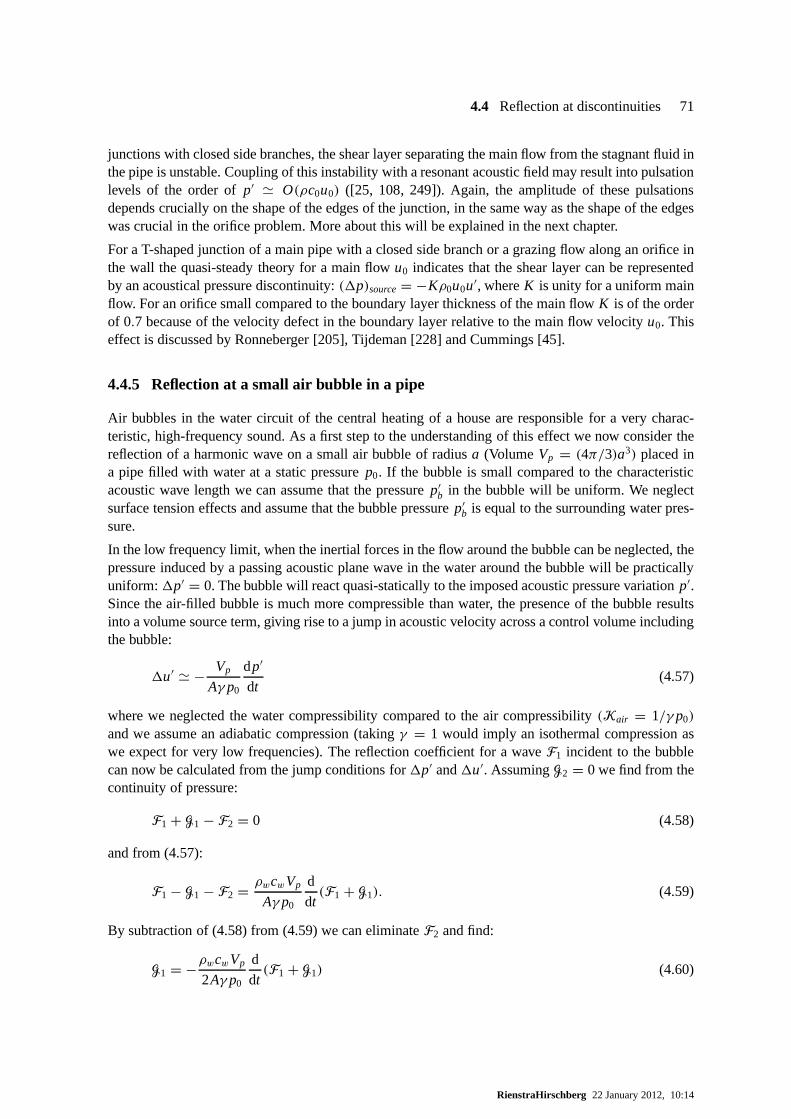
4.4 Reflection at discontinuities 71
junctions with closed side branches, the shear layer separating the main flow from the stagnant fluid inthe pipe is unstable. Coupling of this instability with a resonant acoustic field may result into pulsationlevels of the order ofp′ ' O(ρc0u0) ([25, 108, 249]). Again, the amplitude of these pulsationsdepends crucially on the shape of the edges of the junction, in the same way as the shape of the edgeswas crucial in the orifice problem. More about this will be explained in the next chapter.
For a T-shaped junction of a main pipe with a closed side branch or a grazing flow along an orifice inthe wall the quasi-steady theory for a main flowu0 indicates that the shear layer can be representedby an acoustical pressure discontinuity:(1p)source= −Kρ0u0u′, whereK is unity for a uniform mainflow. For an orifice small compared to the boundary layer thickness of the main flowK is of the orderof 0.7 because of the velocity defect in the boundary layer relative to the main flow velocityu0. Thiseffect is discussed by Ronneberger [205], Tijdeman [228] and Cummings [45].
4.4.5 Reflection at a small air bubble in a pipe
Air bubbles in the water circuit of the central heating of a house are responsible for a very charac-teristic, high-frequency sound. As a first step to the understanding of this effect we now consider thereflection of a harmonic wave on a small air bubble of radiusa (Volume Vp = (4π/3)a3) placed ina pipe filled with water at a static pressurep0. If the bubble is small compared to the characteristicacoustic wave length we can assume that the pressurep′
b in the bubble will be uniform. We neglectsurface tension effects and assume that the bubble pressurep′
b is equal to the surrounding water pres-sure.
In the low frequency limit, when the inertial forces in the flow around the bubble can be neglected, thepressure induced by a passing acoustic plane wave in the water around the bubble will be practicallyuniform:1p′ = 0. The bubble will react quasi-statically to the imposed acoustic pressure variationp′.Since the air-filled bubble is much more compressible than water, the presence of the bubble resultsinto a volume source term, giving rise to a jump in acoustic velocity across a control volume includingthe bubble:
1u′ ' − Vp
Aγ p0
dp′
dt(4.57)
where we neglected the water compressibility compared to the air compressibility(Kair = 1/γ p0)
and we assume an adiabatic compression (takingγ = 1 would imply an isothermal compression aswe expect for very low frequencies). The reflection coefficient for a waveF1 incident to the bubblecan now be calculated from the jump conditions for1p′ and1u′. AssumingG2 = 0 we find from thecontinuity of pressure:
F1 + G1 − F2 = 0 (4.58)
and from (4.57):
F1 − G1 − F2 = ρwcwVp
Aγ p0
d
dt(F1 + G1). (4.59)
By subtraction of (4.58) from (4.59) we can eliminateF2 and find:
G1 = −ρwcwVp
2Aγ p0
d
dt(F1 + G1) (4.60)
RienstraHirschberg 22 January 2012, 10:14
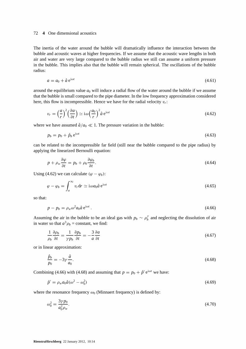
72 4 One dimensional acoustics
The inertia of the water around the bubble will dramaticallyinfluence the interaction between thebubble and acoustic waves at higher frequencies. If we assume that the acoustic wave lengths in bothair and water are very large compared to the bubble radius we still can assume a uniform pressurein the bubble. This implies also that the bubble will remain spherical. The oscillations of the bubbleradius:
a = a0 + a eiωt (4.61)
around the equilibrium valuea0 will induce a radial flow of the water around the bubble if we assumethat the bubble is small compared to the pipe diameter. In thelow frequency approximation consideredhere, this flow is incompressible. Hence we have for the radial velocity vr :
vr =(a
r
)2(∂a
∂t
)' iω
(a0
r
)2a eiωt (4.62)
where we have assumeda/a0 � 1. The pressure variation in the bubble:
pb = p0 + pb eiωt (4.63)
can be related to the incompressible far field (still near thebubble compared to the pipe radius) byapplying the linearized Bernoulli equation:
p + ρw∂ϕ
∂t= pb + ρ0
∂ϕb
∂t. (4.64)
Using (4.62) we can calculate(ϕ − ϕb):
ϕ − ϕb =∫ ∞
avr dr ' iωa0a eiωt (4.65)
so that:
p − pb = ρwω2a0a eiωt . (4.66)
Assuming the air in the bubble to be an ideal gas withpb ∼ ργ
b and neglecting the dissolution of airin water so thata3ρb = constant, we find:
1
ρb
∂ρb
∂t= 1
γ pb
∂pb
∂t= −3
a
∂a
∂t(4.67)
or in linear approximation:
pb
p0= −3γ
a
a0. (4.68)
Combining (4.66) with (4.68) and assuming thatp = p0 + p′ eiωt we have:
p′ = ρwa0a(ω2 − ω20) (4.69)
where the resonance frequencyω0 (Minnaert frequency) is defined by:
ω20 = 3γ p0
a20ρw
. (4.70)
RienstraHirschberg 22 January 2012, 10:14

4.4 Reflection at discontinuities 73
The reflection coefficientR = G1/F1 can now be calculated in a similar way as from (4.58) and (4.59)with the modified source term1u′ = 4π iωa2
0a A−1 eiωt . Since1p′ = 0, we have:
F1 + G1 − F2 = 0 (4.71a)
and
F1 − G1 − F2 = ρwcw4π iωa0(F1 + G1)
Aρw(ω2 − ω20)
(4.71b)
or
R = G1
F1= −
(1 + A(ω2 − ω2
0)
2π iωcwa0
)−1. (4.72)
We see that at resonanceω = ω0 the wave is fully reflected by the bubble, and the reflection coefficientis R = −1. We have of course obtained such a dramatic result because we have neglected all thedissipation mechanisms which can limit the amplitude of thebubble oscillation. The compressibilityof the water flow around the bubble yields already such a mechanism which limits the amplitude of theoscillation at the resonance frequencyω0. This is, however, only one of the many amplitude-limitingmechanisms.
For small bubbles, when the diffusion length for heat transfer into the bubble is comparable to the bub-ble radius, heat transfer is a significant energy loss [177].This occurs for:a = O((Kair/ωρairCP)
1/2).For larger bubbles heat transfer is negligible. For smallerbubbles the compression occurs isothermallyand one should putγ = 1 in the theory. However, the change ofγ from 1.4 to 1 does not introducedamping. It is only in the intermediate range that the heat flux results in a significant rate of vol-ume change in phase with the acoustic pressure. (As it is the work W =
∫p′dV =
∫ T0 p′(dV/dt)dt
which determines the losses, a volumeV proportional top′ implies for a periodic oscillationW ∼∫ T0 p′(dp′/dt)dt = 0.)
Another limitation of the amplitude of the oscillation is the highly non-linear behaviour of the pres-sure for oscillation amplitudesa comparable toa0. If a → 0 the pressure in the bubble increasesdramatically(pb ∼ a−3γ ). Linear theory fails and the bubble may start showing chaotic behaviour(referred to as acoustical chaos) [113].
As an isolated air bubble already has a strong effect on the acoustics of a water filled tube, a largeamount of bubbles will have a dramatic effect. In section 2.3we already considered the low frequencylimit for the speed of sound in a bubbly liquid. We have seen that a small volume fraction of bubblescan considerably reduce the speed of sound. This is due to thelarge compressibility of the air in thebubbles. Asω reachesω0 this effect will become dramatic resulting in a full reflection of the waves(speed of sound zero) [42, 100]. In the frequency rangeω0 < ω < ω0cw/cair no wave propagation ispossible in an ideal bubbly liquid. Above the anti-resonance frequencyω0cw/cair the bubble movementis in opposition to the applied pressure fluctuations. The radius increases when the pressure increases.This is just opposite to the low frequency behaviour (figure 4.11). As a result the bubbly mixture willbe stiffer than water, andc > cw! Sound speeds of up to 2500 m/s were indeed observed in bubblywater withβ = 2 × 10⁻⁴ !
Another fascinating effect of bubble resonance is its role in the very specific, universal, sound thatrain is known to generate when it hits a water surface [178]. First it should be noted that bubbleoscillation is such an efficient source of sound that any rainimpact sound is dominated by it. Now, inspite of the wide range of velocities and sizes of rain drops that occurs, the universality of the sound
RienstraHirschberg 22 January 2012, 10:14
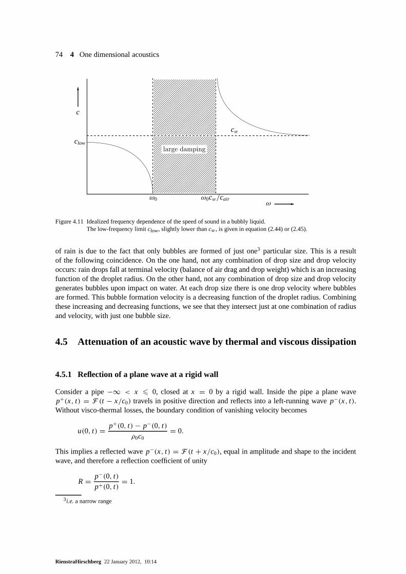
74 4 One dimensional acoustics
123456789012345678901234567890123456789012345678901234567890123456789012345678901234567890123456789012345678901234567890123456789012345678901234567890123456789012345678901234567890123456789012345678901234567890123456789012345678901234567890123456789012345678901234567890123456789012345678901234567890123456789012345678901234567890123456789012345678901234567890123456789012345678901234567890123456789012345678901234567890123456789012345678901234567890123456789012345678901234567890123456789012345678901234567890123456789012345678901234567890123456789012345678901234567890123456789012345678901234567890123456789012345678901234567890123456789012345678901234567890123456789012345678901234567890123456789012345678901234567890123456789012345678901234567890123456789012345678901234567890123456789012345678901234567890
1
123456789012345678901234567890123456789012345678901234567890123456789012345678901234567890123456789012345678901234567890123456789012345678901234567890123456789012345678901234567890123456789012345678901234567890123456789012345678901234567890123456789012345678901234567890123456789012345678901234567890123456789012345678901234567890123456789012345678901234567890123456789012345678901234567890123456789012345678901234567890123456789012345678901234567890123456789012345678901234567890123456789012345678901234567890123456789012345678901234567890123456789012345678901234567890123456789012345678901234567890123456789012345678901234567890123456789012345678901234567890123456789012345678901234567890123456789012345678901234567890123456789012345678901234567890123456789012345678901234567890123456789012345678901234567890123456789012345678901234567890
c
6
cw
clowlarge damping
ω0 ω0cw/cairω -
Figure 4.11 Idealized frequency dependence of the speed of sound in a bubbly liquid.The low-frequency limitclow, slightly lower thancw , is given in equation (2.44) or (2.45).
of rain is due to the fact that only bubbles are formed of just one3 particular size. This is a resultof the following coincidence. On the one hand, not any combination of drop size and drop velocityoccurs: rain drops fall at terminal velocity (balance of airdrag and drop weight) which is an increasingfunction of the droplet radius. On the other hand, not any combination of drop size and drop velocitygenerates bubbles upon impact on water. At each drop size there is one drop velocity where bubblesare formed. This bubble formation velocity is a decreasing function of the droplet radius. Combiningthese increasing and decreasing functions, we see that theyintersect just at one combination of radiusand velocity, with just one bubble size.
4.5 Attenuation of an acoustic wave by thermal and viscous dissipation
4.5.1 Reflection of a plane wave at a rigid wall
Consider a pipe−∞ < x 6 0, closed atx = 0 by a rigid wall. Inside the pipe a plane wavep+(x, t) = F (t − x/c0) travels in positive direction and reflects into a left-running wavep−(x, t).Without visco-thermal losses, the boundary condition of vanishing velocity becomes
u(0, t) = p+(0, t) − p−(0, t)
ρ0c0= 0.
This implies a reflected wavep−(x, t) = F (t + x/c0), equal in amplitude and shape to the incidentwave, and therefore a reflection coefficient of unity
R = p−(0, t)
p+(0, t)= 1.
3i.e.a narrow range
RienstraHirschberg 22 January 2012, 10:14
4.5 Attenuation of an acoustic wave by thermal and viscous dissipation 75
In reality unsteady heat transfer at the wall will act as a sink of sound, slightly reducing the reflectioncoefficient. This heat transfer is a result from the difference between the wall temperatureTw, whichremains practically constant, and the bulk temperatureT of the gas, which varies with the adiabaticpressure fluctuationsp′ = p+ + p−. We will limit our analysis to small temperature differences(T − Tw) and small departures from the quiescent reference state. This allows a linearized theory, sothat we can consider the reflection of a harmonic wave, denoted in complex form as
p(x, t) = p(x)e−iωt
with amplitude p outside the neighbourhood of the wall being given byp(x) = p+ e−ikx + p− eikx.(Likewise, in the following the hatted quantities with “ˆ ” will denote their corresponding,x-dependent, complex amplitudes.)
We define(see also section 8.8) the thermal boundary layer thicknessδT as the width of the regionnear the wall in which the rate of increase of internal energyis just balancing the net rate of heatconduction (in this region the wave equation is not valid):
(ρ0Cp
∂
∂tT ∼ ωρ0CpT ′
)'
(K0
∂2
∂x2T ∼ K0
T ′
δ2T
).
Hence, the characteristic length scale for the thermal boundary layer is
δT =√
2K0
ωρ0Cp. (4.73)
We will now calculate the temperature profile within the thermal boundary layer. This will allow us tocalculate the deviationρe = ρ − p/c2
0 between the density fluctuations in the boundary layer and thedensity fluctuationsp/c2
0 corresponding to adiabatic compression of an ideal acoustic flow as foundoutside the boundary layer. This excess densityρe has to be supplied by a fluid flow towards thewall at the edge of the boundary layer. This velocityu∞ can be interpreted by an observer, outsidethe boundary layer, as due to a displacementdT of the rigid wall in a hypothetical fluid without heatconduction. The work performed by this “virtual” wall displacement on the acoustic field correspondsto the sound dissipation by the thermal conduction in the boundary layer.
This approximation is based on the key assumption that the acoustic wave length is much larger thanthe thicknessδT of the thermal boundary layer:ωδT/c0 � 1. In such a case we can assume at the edgeof the boundary layer a uniform adiabatic flow,(du/dx)∞ = 0, of a uniform fluid (p∞, ρ∞). The non-uniformity associated with the acoustic wave propagation is negligible on the length scale we consider.The boundary layer flow is described by the one-dimensional conservation laws (1.1,1.2,1.6,1.7) inlinearized form:
iωρ = −ρ0du
dx, (4.74a)
iωρ0u = −dp
dx+ 4
3η0
d2u
dx2, (4.74b)
iωCVρ0T = −p0du
dx+ K0
d2T
dx2. (4.74c)
Since in a liquid acoustic wave propagation is isothermal wecan limit our analysis to a gas. We assumean ideal gas with:
p
p0= ρ
ρ0+ T
T0.
RienstraHirschberg 22 January 2012, 10:14
76 4 One dimensional acoustics
The boundary conditions are given by:
T(0) = Tw, u(0) = 0,T∞T0
= γ − 1
γ
p∞p0,
p(x) → p∞ = p+ + p− (x/δT → −∞),
where we have introduced, for generality, the fluctuation ofthe wall temperatureTw. After the studyof the reflection of a wave at an isothermal wall (Tw = 0) we can use the same theory to calculate thesound generated by fluctuations of the wall temperature (Tw 6= 0).
After eliminating u from the energy equation by using the mass conservation law,and eliminatingρby means of an ideal gas law, we obtain
iω( T
T0− γ − 1
γ
p
p0
)= a0
d2
dx2
( T
T0
)
wherea0 = K0/ρ0Cp is the heat diffusivity coefficient. In terms of the excess density, with
ρe
ρ0= 1
ρ0
(ρ − p
c20
)= ρ
ρ0− p
γ p0= γ − 1
γ
p
p0− T
T0,
this equation becomes
iωρe
ρ0= a0
d2
dx2
( ρe
ρ0
)− a0
γ − 1
γ
d2
dx2
( p
p0
).
Combining the momentum and mass conservation laws we have
ω2ρ = −d2 p
dx2+ 4
3η0
d3u
dx3.
Assuming that viscosity is not dominant – which we can check from the solution to be obtained – wesee that
d2
dx2
( p
p0
)' −ω
2ρ
p0= −ω
2γ
c20
ρ
ρ0.
The relative pressure variation across the boundary layer (4.73) is of the order of
p − p∞p0
∼ ω2δ2T
c20
( ρρ0
)
while ρe/ρ0 is of the same order of magnitude asρ/ρ0, becauseγ − 1 = O(1). This implies that ifwe neglect terms of the order ofω2δ2
T/c20, we have
iωρe
ρ0= a0
d2
dx2
( ρe
ρ0
).
This equation has the solution
ρe
ρ0=
[ρe
ρ0
]
w
exp((1 + i )x/δT
)(4.75)
where
[ρe
ρ0
]
w
= γ − 1
γ
p∞p0
− TwT0.
RienstraHirschberg 22 January 2012, 10:14
4.5 Attenuation of an acoustic wave by thermal and viscous dissipation 77
Using the equation of mass conservation, the velocityu(−δT ) at the edge of the boundary layer isgiven by the integral of the density across the boundary layer as follows. (Note that we have chosenthe positivex-direction towards the wall.)
u(0)− u(−δT ) = −iω∫ 0
−δT
ρ
ρ0dx.
The difference between this velocity and the velocity−iω(ρ∞/ρ0)δT that would occur in the absenceof heat conduction, can be interpreted as a fictitious wall velocity uT given by
uT = iωdT = iω∫ 0
−δT
ρ − ρ∞ρ0
dx = iω∫ 0
−∞
ρe
ρ0dx,
wheredT is the fictitious wall displacement amplitude. Substitution of solution (4.75) yields
dT = 12(1 − i )δT
[ ρe
ρ0
]w, (4.76a)
= 12(1 − i )δT
γ − 1
γ
p∞p0
if Tw = 0 (an isothermal wall). (4.76b)
For an isothermal wall (Tw = 0) these wall effects, leading to the effective velocityuT , have thesame effect to the incident acoustic wave as an impedance of the wall. This equivalent impedanceZT , defined as the ratio of the acoustic pressure fluctuationsp∞ at the wall and the flow velocityuT
directed towards the wall (c.f. Eq. 3.14), is then given by
ZT = p∞uT
= p∞
iωdT
= ρ0c0(1 − i )c0
(γ − 1)ωδT
The corresponding time averaged acoustic intensity is found to be
〈IT 〉 = 〈p′u′〉 = 12 Re(1/ZT )| p∞|2 = 1
4(γ − 1)ωδT
ρ0c20
| p∞|2
which indicates an energy flux from the acoustic field towardsthe wall and therefore an absorption ofenergy.
4.5.2 Viscous laminar boundary layer
The viscous attenuation of a plane acoustic wave propagating along a pipe can often be describedin a similar way as the thermal attenuation by means of a displacement thicknessdV of the wall. Weconsider first the simple case of a laminar boundary layer in the case of wave propagation in a stagnantand uniform fluid. The wave propagates in thex-direction and induces an acoustic velocity parallel tothe wall which has an amplitudeu∞ in the bulk of the flow. The no-slip condition at the wall,uw = 0,induces a viscous boundary layer of thickness
δV =√
2ν0/ω = δT
√Pr . (4.77)
RienstraHirschberg 22 January 2012, 10:14
78 4 One dimensional acoustics
wherePr = ν0ρ0Cp/K0 is Prandtl’s number. This viscous boundary layer is usuallyreferred to as theStokes layer. Neglecting terms of the order of(ωδV/c0)
2 we can write thex-momentum conservationlaw in the boundary layer as
iωρ0u = η0d2u
dy2,
wherey is the direction normal to and towards the wall (soy ≤ 0). They-momentum conservationlaw reduces to the pressure being uniform across the viscousboundary layer. The boundary conditionsare
u(0) = uw = 0, u(y) → u∞ if y/δV → −∞.
The solution is then
u = u∞
[1 − exp
((1 + i )y
δV
)]. (4.78)
The displacement thicknessdV is defined as the fictitious wall position for which the acoustical massflux of a uniform flow with the velocityu∞ is equal to the actual mass flow. This implies:
dV =∫ ∞
0
(1 − u
u∞
)dy = −1
2(1 − i )δV . (4.79)
4.5.3 Damping in ducts with isothermal walls.
In section 4.5.1 we have considered the attenuation of an acoustic wave that reflects normally to a wall.This attenuation was due to the heat conduction in the thermal boundary layer. In the previous section4.5.2 we have described the laminar viscous boundary layer associated to a plane wave propagatingalong a duct (parallel to the wall). In a gas such a propagation will also induce a thermal boundarylayer, determined by the pressure fluctuationsp′
∞ in the bulk of the flow. The expression for thedisplacement thicknessdT derived in section 4.5.1 can be applied.
Using the concept of displacement thickness we will calculate the attenuation of a plane wave travel-ling in x-direction along a pipe of cross-sectional areaA and cross-sectional perimeterL p. We assumethat the boundary layers are thin compared to the pipe diameter.
The bulk of the flow is described by the following plane wave, satisfying Euler’s equation in linearapproximation:
p′∞ = p∞ eiωt−ikx, iωρ0u
′∞ = i kp′
∞,
wherek is a complex wave number (the imaginary part will describe the attenuation). Incorporatingthe displacement thickness to the mass conservation law integrated over the pipe cross section yields(Lighthill [121])
∂
∂t
[ρ∞(A + L pdT )
]= ∂
∂x
[ρ∞u∞(A + L pdV )
]
In linear approximation for a harmonic wave this becomes
iω( p∞
c20
A + ρ0L pdT
)= i kρ0u∞(A + L pdV)
RienstraHirschberg 22 January 2012, 10:14

4.5 Attenuation of an acoustic wave by thermal and viscous dissipation 79
where we made use of the isentropic relationshipp∞ = c20ρ∞. After substitution of the expressions
for the displacement thicknessdT (4.76b) anddV (4.79)
dT = 12(1 − i )δT
γ − 1
γ
p∞p0, and dV = −1
2(1 − i )δV ,
and elimination ofu∞ by means of the Euler’s equation, we find a homogeneous linearequation forp∞, which yields the dispersion relation
k2
k20
=A + 1
2(1 − i )(γ − 1)L pδT
A − 12(1 − i )L pδV
,
wherek0 = ω/c0. Expanding this expression for smallδT andδV (using the fact thatδV/δT =√
Pr =O(1)) and retaining the first order term, we obtain the result of Kirchhoff
k − k0 = 14(1 − i )
L p
AδVk0
(1 + (γ − 1)
δT
δV
), (4.80)
which corresponds to equation (2.13). More accurate expressions at low frequencies, when the acous-tical boundary layers are not thin, are discussed by Tijdeman [227] and Kergomard [104]. At highfrequencies the viscosity becomes significant also in the bulk of the flow (Pierce [173]).
At high amplitudes (u∞δV/ν ≥ 400) the acoustical boundary layer becomes turbulent (Merkli [133],Eckmann [55], Akhavan [3], Verzicco [235]). In such a case the damping becomes essentially non-linear. Akhavan [3] presents results indicating that a quasi-stationary turbulent flow model provides afair first guess of the wall shear stress.
For an isothermal (liquid) flow the quasi-steady approximation yields
k2 − k20 = −1
4 i k0L p
Ac f u∞
where the friction coefficientc f is defined (and determined) by
c f = − 4A
L p12ρ0U2
0
dp0
dx
which relates the mean pressure pressure gradient (dp0/dx) to the stagnation pressure12ρ0U20 of a
mean flow through the pipe. Note that since(k − k0) depends on the amplitudeu∞ of the acousticalvelocity this model implies a non-linear damping. The transition from laminar to turbulent dampingcan therefore be a mechanism for saturation of self-sustained oscillations (see chapter 5).
For smooth pipes, Prandtl proposed a correlation formula for c f as a function of the Reynolds num-ber of the flow. The influence of wall roughness is described inthe Moody diagram. Such data arediscussed by Schlichting [214]. In the case of a turbulent gas flow the thermal dissipation is rathercomplex. This makes a low frequency limit difficult to establish. In the presence of a mean flow var-ious approximations describing the interaction between the acoustic waves and the turbulent mainflow have been discussed by Ronneberger [206] and Peters [171]. The formula of Kirchhoff derivedabove appears to be valid at low Mach numbers (U0/c0 � 1) as long as the Stokes viscous boundarylayer thicknessδV remains less than the laminar sublayerδL ' 15ν/
√τwρ0 of the turbulent main flow
(where the wall shear stressτw = c f18ρ0U2
0 ).
WhenδL � δV , we can use a quasi-stationary approximation. The transition from the high frequencylimit to the quasi-stationary limit is discussed in detail by Ronneberger [206] and Peters [170].Thesereferences also provide information about the Mach number dependence of the wave number.
RienstraHirschberg 22 January 2012, 10:14

80 4 One dimensional acoustics
4.6 One dimensional Green’s function
4.6.1 Infinite uniform tube
We consider a one dimensional approximation for the propagation of waves in a pipe. This approxi-mation will be valid only if the frequencies generated by thesources of sound in the pipe are lowerthan the cut-off frequency. As the acoustic field observed atpositionx far from a source placed aty isinduced by a plane wave, the observer position in the cross section of the pipe is indifferent. Apply-ing the reciprocity principle (section 3.1) we see that in the low frequency approximation the signalobserved atx should also be indifferent for the position of the source in the cross section of the tubeat y. Hence as the source position within a cross section is indifferent we can consider the source tobe smeared out over this cross section resulting in a 1-dimensional source. We therefore look for thecorresponding one-dimensional Green’s functiong(x, t|y, τ ) defined by:
∂2g
∂t2− c2
0∂2g
∂x2= δ(t − τ)δ(x − y). (4.81)
Comparison of this wave equation with the wave equation (4.5) in the presence of source termρ0∂β/∂tand forcesfx:
∂2p′
∂t2− c2
0∂2 p′
∂x2= c2
0
(ρ0∂2β
∂t2− ∂ fx
∂x
)(4.5)
indicates that we can assume that (4.81) is a particular caseof (4.5) for fx = 0 and:
∂β
∂t= 1
ρ0 c20
H (t − τ)δ(x − y). (4.82)
For an infinitely long tube the solution is:
g(x, t|y, τ ) =
1
2c0H
(t − τ + x − y
c0
)for x < y,
1
2c0H
(t − τ − x − y
c0
)for x > y.
(4.83)
This result is obtained intuitively by using (4.30) which implies thatg is the pressure wave generatedby a piston moving with a velocityu′ = (2ρ0c2
0)−1H (t − τ) for x = y + ε and a second piston with
a velocityu′ = −(2ρ0c20)
−1H (t − τ) for x = y − ε. Equations (4.83) are then obtained by using themethod of characteristics (section 4.2).
Of course, the above result (4.83) is more efficiently written as:
g(x, t|y, τ ) = 1
2c0H
(t − τ − |x − y|
c0
). (4.84)
The combinationt − |x − y|/c0 is the time at which the signal observed at(x, t) has been emitted bythe source aty. This time is called the retarded or emission timete:
te = t − |x − y|c0
. (4.85)
RienstraHirschberg 22 January 2012, 10:14

4.7 Aero-acoustical applications 81
4.6.2 Finite uniform tube
We can also fairly easily construct a Green’s function for a semi-infinite pipe (x < L) terminatedat x = L by an ideal open end at which by definitiong(L , t|y, τ ) = 0. By constructing the wavereflecting at this ideal open end with the method of characteristics we find:
g(x, t|y, τ ) = 1
2c0
{H
(t − τ + x − y
c0
)+ H
(t − τ − x − y
c0
)
−H(t − τ + x + y − 2L
c0
)}(4.86)
which we can also write forx < L as:
g(x, t|y, τ ) = 1
2c0
{H
(t − τ − |x − y|
c0
)− H
(t − τ − |x + y − 2L|
c0
)}. (4.87)
This solution could also have been obtained by assuming the pipe to be part of an infinitely longpipe, in which at the pointx = 2L − y a second point source is placed with opposite sign of andsynchronous with the original point source atx = y. This second source, calledimage source, isconstructed such that it generates the field due to reflectionby the boundary atx = L in the originalproblem, and therefore brings into effect the boundary condition at x = L. Thismethod of imagescanbe generalized to the case of a finite pipe segment (0< x < L). In such a case we will have to considerthe contribution of an infinite number of images corresponding to the reflections of the original wavesat the boundaries. For example, the field in a finite pipe with hard walled ends is equivalent with thefield in an infinite pipe with equal sources inx = −y, ±2L ± y, ±4L ± y, . . . . This comes down toa right-hand-side of equation 4.81 of
∞∑
n=−∞δ(t − τ)
(δ(x − y − 2nL)+ δ(x + y − 2nL)
)
and a solution
g(x, t|y, τ ) = 1
2c0
∞∑
n=−∞
{H
(t − τ − |x − y − 2nL|
c0
)+ H
(t − τ − |x + y − 2nL|
c0
)}.
(4.88)
The Green’s function is clearly more complex now. Furthermore, the addition of mass by the sourcein the finite volume results into a (roughly) linear growth ofg in t . (Verify this for x = y = 1
2 L andτ = 0.) This is of particular interest in the time-harmonic case. When the end conditions are such thatmultiple reflections are physically relevant they imply that constructive and destructive interferenceswill select waves corresponding to standing wave patterns or resonances of the tube. This problemwill be discussed further in the next chapter.
4.7 Aero-acoustical applications
4.7.1 Sound produced by turbulence
We consider a turbulent jet in an infinitely extended pipe (figure 4.12). We suppose that the jet diameter
RienstraHirschberg 22 January 2012, 10:14
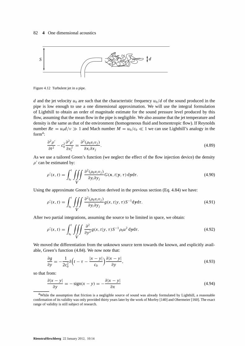
82 4 One dimensional acoustics
S
6
?
d6?
Figure 4.12 Turbulent jet in a pipe.
d and the jet velocityu0 are such that the characteristic frequencyu0/d of the sound produced in thepipe is low enough to use a one dimensional approximation. Wewill use the integral formulationof Lighthill to obtain an order of magnitude estimate for thesound pressure level produced by thisflow, assuming that the mean flow in the pipe is negligible. We also assume that the jet temperature anddensity is the same as that of the environment (homogeneous fluid and homentropic flow). If ReynoldsnumberRe = u0d/ν � 1 and Mach numberM = u0/c0 � 1 we can use Lighthill’s analogy in theform4:
∂2ρ ′
∂t2− c2
0∂2ρ ′
∂x2i
= ∂2(ρ0vi v j )
∂xi ∂x j. (4.89)
As we use a tailored Green’s function (we neglect the effect of the flow injection device) the densityρ ′ can be estimated by:
ρ ′(x, t) =∫ t
t0
∫∫∫
V
∂2(ρ0vi v j )
∂yi∂y jG(x, t|y, τ )dydτ. (4.90)
Using the approximate Green’s function derived in the previous section (Eq. 4.84) we have:
ρ ′(x, t) =∫ t
t0
∫∫∫
V
∂2(ρ0vi v j )
∂yi∂y jg(x, t|y, τ )S−1dydτ. (4.91)
After two partial integrations, assuming the source to be limited in space, we obtain:
ρ ′(x, t) =∫ t
t0
∫∫∫
V
∂2
∂y2g(x, t|y, τ )S−1ρ0u
2 dydτ. (4.92)
We moved the differentiation from the unknown source term towards the known, and explicitly avail-able, Green’s function (4.84). We now note that:
∂g
∂y= − 1
2c20
δ(t − τ − |x − y|
c0
)∂|x − y|∂y
, (4.93)
so that from:
∂|x − y|∂y
= − sign(x − y) = −∂|x − y|∂x
(4.94)
4While the assumption that friction is a negligible source ofsound was already formulated by Lighthill, a reasonableconfirmation of its validity was only provided thirty years later by the work of Morfey [140] and Obermeier [160]. The exactrange of validity is still subject of research.
RienstraHirschberg 22 January 2012, 10:14

4.7 Aero-acoustical applications 83
we have the following important symmetry in the Green’s function of an infinite pipe:
∂g
∂y= −∂g
∂x. (4.95)
We substitute this result in (4.92). Since the integration is to the source positiong, we can now removeone of the differentiations tox from the integral, resulting in the expression:
ρ ′(x, t) = ∂
∂x
∫ t
t0
∫∫∫
V
ρ0u2
2Sc20δ(te − τ) sign(x − y)dydτ. (4.96)
with te = t − |x − y|/c0. The time integration can now be carried out:
ρ ′(x, t) = ∂
∂x
∫∫∫
V
1
2Sc20[ρ0u
2]τ=te sign(x − y)dy (4.97)
where we used the property (C.26) of theδ-function. At sufficiently large distances the only lengthscale in the solution is the characteristic wave lengthc0d/u0 corresponding to the characteristic fre-quency5 u0/d of the turbulence in the jet. Hence we can estimate:
∂
∂x' 1
c0
∂
∂t∼ u0
c0d= M0
d. (4.98)
Because the sound production by turbulence decreases very fast with decreasing mean flow velocity,the volume of the free jet contributing to the sound production is limited to a region of the order ofd3. In this region the turbulent velocity fluctuations are of the order ofu0. Hence we find at largedistances:
ρ ′ ∼ M0
d
ρ0u20
2Sc20d3 (4.99)
implying:
ρ ′2 ∼(1
2ρ0M3
0d2/S)2. (4.100)
This is the result obtained by Ffowcs Williams [63]. This Mach number dependence has indeed beenobserved in a pipe downstream of an orifice for sufficiently high Mach numbers. At low Mach numbersthe sound production is dominated by the dipole contribution of O(M4) due to the interaction of theflow with the orifice [134].
A discussion of the sound production by confined circular jets is provided by Reethof [184] for ar-bitrary jet Mach numbers. Reethof finds for subsonic jets (M0 < 1) a ratio of the radiated powerto the flow powerηac = 3 × 10⁻⁴M3
0 . For supersonic jets (M0 > 1) typical values areηac =1.6 × 10⁻³(M2
0 − 1)1/2. In that case the Mach number is taken fromM20 = 2
γ−1[(p1/p2)(γ−1)/γ − 1],
wherep1/p2 is the ratio of the pressure across the orifice.
The dependence of the sound production on the jet geometry isdiscussed by Verge [234] andHirschberg [78]. For planar jets issued from a slit of heighth the typical frequencies are of theorder of 0.03u0/h (Bjørnø [15], Sato [213]). This implies that correlations developed for subsoniccircular jets are useless for planar jets.
5We assume a jet with circular cross section.
RienstraHirschberg 22 January 2012, 10:14

84 4 One dimensional acoustics
4.7.2 An isolated bubble in a turbulent pipe flow
Consider an isolated bubble of radiusa0 small compared to the pipe diameterD. Assume a turbulentpipe flow. The sound produced by the turbulence will, locally, be enhanced by the presence of thebubble. If we assume that the frequencies in the turbulence,typically O(u0/D), are much smallerthan the bubble resonance frequencyω0, we can calculate the sound produced by the interaction ofthe bubble with the turbulence.
The Green’s function is calculated by using the reciprocityprinciple. We consider the acoustic re-sponse of the bubble for a plane wave emitted from the observer positionx towards the bubble. Forthe sake of simplicity we consider this incident wave to be harmonic pin = pin eiωt−ikx. The bubblepressure responsepb is, as is shown in 5.4.5 (use (4.72) withpin = F1 and p′ = F2), given by:
pb = −
(ω0
ω
)2
1 −(ω0
ω
)2− 2π i a0cw
Sω
pin. (4.101)
Using Bernoulli and the continuity equation we can calculate the pressure distribution around thebubble:
p − pb = −ρwiω(ϕ − ϕb) (4.102)
where:
ϕ − ϕb =∫ r
a0
iωaa20
r 2dr = iωaa0
(1 − a0
r
). (4.103)
Furthermore, we have:
a
a0= − pb
3γ p0, (4.104)
so thatp(r ) is given by:
p = pb
(1 −
( ωω0
)2(1 − a0
r
))=
1 −(ω0
ω
)2− a0
r
1 −(ω0
ω
)2− 2π i a0cw
Sω
pin. (4.105)
Taking for pin the Fourier transform of(2c0S)−1H (t − τ − |x − y|/c0) we obtain asp the FouriertransformG(x|y) of the Green’s functionG(x, t|y, τ ):
G(x|y) = e−iωτ−ik|x−y|
2iωcwS·
1 −(ω0
ω
)2− a0
r
1 −(ω0
ω
)2− 2π i a0cw
Sω
. (4.106)
Using Lighthill’s analogy we now can compare the response ofthe pipe to turbulence, with and with-out bubble. We obtain by partial integration:
ρ ′ =∫ t
t0
∫∫∫
V
ρ0vi v j∂2G
∂yi∂y jdydτ. (4.107)
RienstraHirschberg 22 January 2012, 10:14
4.7 Aero-acoustical applications 85
If we consider a small turbulent spot in the direct neighbourhood of the bubble the ratio of the re-sponses is given by:
∂2Gb
∂r 2
∂2G0
∂y2
=
∂2Gb
∂r 2
∂2G0
∂x2
=
c2wa0
ω2r 3
1 −(ω0
ω
)2− 2π i a0cw
Sω
. (4.108)
At the resonance frequencyω0 this yields a factor(a0S/4πr 3)(ρwc2w/3γ p0)
12 while for low fre-
quencies we find(a0/r )3(ρwc2w/3γ p0). If r = O(a0) we see that the sound produced by turbulence in
the neighbourhood of the bubble will be dramatically enhanced.
The major contribution of the bubble turbulence interaction will be at low frequencies. An importantreason for this is that for typical conditions in water flow, the length scale of vortices correspondingto pressure fluctuations at the bubble resonance frequencyω0/2π is much smaller than the bubbleradius [43]. In such a case these pressure fluctuations are averaged out at the bubble surface and donot have any significant contribution to the spherical oscillations of the bubble. An example of soundproduction by bubbles in a pipe flow is the typical sound of a central heating system when air ispresent in the pipes. Also the romantic sound of water streams and fountains is dominated by bubbles.In those cases, however, we have a three-dimensional environment.
4.7.3 Reflection of a wave at a temperature inhomogeneity
As a last example of the use of the integral equation based on the Green’s function formalism weconsider the interaction of a wave with a limited region in which the gas temperatureT(x) is non-uniform (0< x < L). We assume the pipe to be horizontal and that gravity is negligible. Hence, atrest the pressure is uniform. The gas density is given by:
ρ/ρ0 = T/T0 (4.109)
and the speed of soundc is given by:
c/c0 = (T/T0)12 (4.110)
whereρ0, T0 and c0 are the properties of the uniform region. We now further assume that|T −T0|/T0 � 1 so that we can use a linear approximation in which we assume that the scattered soundwave p′′ is weak compared to the amplitudep′
i of the incident wave. In such a case we can writep′ = p′
in + p′′, so that the linearized 1-D wave equation (2.50):
∂2p′
∂t2− ∂
∂x
(c2∂p′
∂x
)= 0
can be approximated by:
∂2p′′
∂t2− c2
0
∂2 p′′
∂x2= ∂
∂x
((c2 − c2
0)∂p′
in
∂x
). (4.111)
The source term has been linearized by assuming that the pressure fluctuations are equal to the (undis-turbed) incident wave amplitude. It is the source term considered by Powell [176] for the descriptionof sound scattering at entropy spots.
RienstraHirschberg 22 January 2012, 10:14
86 4 One dimensional acoustics
Using the integral formulation (3.13) and the one dimensional Green’s functiong we find:
p′′ =∫ ∞
−∞
∫ L
0
∂
∂y(c2 − c2
0)∂p′
in
∂yg dydτ. (4.112)
Partial integration yields
p′′ = −∫ ∞
−∞
∫ L
0(c2 − c2
0)∂p′
in
∂y
∂g
∂ydydτ. (4.113)
From equation (4.84) we have
∂g
∂y= 1
2c20
sign(x − y)δ(te − τ) (4.114)
(with te = t − |x − y|/c0) and hence
p′′ = − 1
2c20
∫ L
0sign(x − y)(c2 − c2
0)
∫ ∞
−∞δ(te − τ)
∂p′in
∂ydτdy
= − 1
2c20
∫ L
0sign(x − y)(c2 − c2
0)∂
∂yp′
in(y, te)dy. (4.115)
If we take for example
p′in = pin H (x − c0t) (4.116)
and use the relationc2/c20 = T/T0, then we have for (say)x < 0
p′′ = 14 pin
∫ L
0
T − T0
T0δ(
y − x + c0t
2
)dy (4.117)
=
14 pin
T(12(x + c0t))− 1
T0if 0 < x + c0t < 2L
0 otherwise.
Exercises
a) Show that for an acoustic wave travelling in the negativex direction we have:
u′ = −p′/ρ0c0.
b) Consider a rigid piston at(x = 0) separating the fluid I forx < 0 from the fluid II atx > 0 in aninfinitely long pipe of 10−2 m2 cross section. Assume that the piston oscillates with a frequencyω andan amplitudea. Calculate the force necessary to move the piston as a function of time (ρ0,I = 1.2kg/m3,c0,I = 344 m/s,ρ0,II = 1.8 kg/m3 andc0,II = 279 m/s,ω = 103 rad/s,a = 10−3 m). Use linear theoryand verify if it is indeed valid.
c) Water hammer effect:Consider a steady flow of water in a rigid horizontal pipe which we stop suddenly by closing a valve.Calculate the pressure on both sides of the valve for flow velocities of 0.01 m/s and 1 m/s. What is theforce on the valve for a pipe cross section surface of 10−2 m2.
RienstraHirschberg 22 January 2012, 10:14
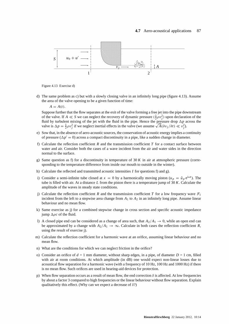
4.7 Aero-acoustical applications 87
1234567890123456789012345678901123456789012345678901234567890112345678901234567890123456789011234567890123456789012345678901123456789012345678901234567890112345678901234567890123456789011234567890123456789012345678901123456789012345678901234567890112345678901234567890123456789011234567890123456789012345678901123456789012345678901234567890112345678901234567890123456789011234567890123456789012345678901123456789012345678901234567890112345678901234567890123456789011234567890123456789012345678901123456789012345678901234567890112345678901234567890123456789011234567890123456789012345678901123456789012345678901234567890112345678901234567890123456789011234567890123456789012345678901123456789012345678901234567890112345678901234567890123456789011234567890123456789012345678901123456789012345678901234567890112345678901234567890123456789011234567890123456789012345678901123456789012345678901234567890112345678901234567890123456789011234567890123456789012345678901123456789012345678901234567890112345678901234567890123456789011234567890123456789012345678901123456789012345678901234567890112345678901234567890123456789011234567890123456789012345678901
123456789012345678901123456789012345678901123456789012345678901123456789012345678901123456789012345678901123456789012345678901123456789012345678901123456789012345678901123456789012345678901123456789012345678901123456789012345678901123456789012345678901123456789012345678901123456789012345678901123456789012345678901123456789012345678901123456789012345678901123456789012345678901123456789012345678901123456789012345678901123456789012345678901123456789012345678901123456789012345678901123456789012345678901123456789012345678901123456789012345678901
S u0 + u′
v j A
1 2
Figure 4.13 Exercise d)
d) The same problem as c) but with a slowly closing valve in an infinitely long pipe (figure 4.13). Assumethe area of the valve opening to be a given function of time:
A = A(t).
Suppose further that the flow separates at the exit of the valve forming a free jet into the pipe downstreamof the valve. IfA � S we can neglect the recovery of dynamic pressure(1
2ρv2j ) upon declaration of the
fluid by turbulent mixing of the jet with the fluid in the pipe. Hence the pressure drop1p across thevalve is1p = 1
2ρv2j if we neglect inertial effects in the valve (we assume
√A(∂v j /∂ t) � v2
j ).
e) Sow that, in the absence of aero-acoustic sources, the conservation of acoustic energy implies a continuityof pressure (1p′ = 0) across a compact discontinuity in a pipe, like a sudden change in diameter.
f) Calculate the reflection coefficientR and the transmission coefficientT for a contact surface betweenwater and air. Consider both the cases of a wave incident fromthe air and water sides in the directionnormal to the surface.
g) Same question as f) for a discontinuity in temperature of 30 K in air at atmospheric pressure (corre-sponding to the temperature difference from inside our mouth to outside in the winter).
h) Calculate the reflected and transmitted acoustic intensities I for questions f) and g).
i) Consider a semi-infinite tube closed atx = 0 by a harmonically moving piston (up = up eiωt ). Thetube is filled with air. At a distanceL from the piston there is a temperature jump of 30K . Calculate theamplitude of the waves in steady state conditions.
j) Calculate the reflection coefficientR and the transmission coefficientT for a low frequency waveF1incident from the left to a stepwise area change fromA1 to A2 in an infinitely long pipe. Assume linearbehaviour and no mean flow.
k) Same exercise as j) for a combined stepwise change in crosssection and specific acoustic impedancejump1ρc of the fluid.
l) A closed pipe end can be considered as a change of area such,that A2/A1 → 0, while an open end canbe approximated by a change withA2/A1 → ∞. Calculate in both cases the reflection coefficientR,using the result of exercise j).
m) Calculate the reflection coefficient for a harmonic wave atan orifice, assuming linear behaviour and nomean flow.
n) What are the conditions for which we can neglect friction in the orifice?
o) Consider an orifice ofd = 1 mm diameter, without sharp edges, in a pipe, of diameterD = 1 cm, filledwith air at room conditions. At which amplitude (in dB) one would expect non-linear losses due toacoustical flow separation for a harmonic wave (with a frequency of 10 Hz, 100 Hz and 1000 Hz) if thereis no mean flow. Such orifices are used in hearing-aid devices for protection.
p) When flow separation occurs as a result of mean flow, the end correctionδ is affected. At low frequenciesby about a factor 3 compared to high frequencies or the linearbehaviour without flow separation. Explainqualitatively this effect. (Why can we expect a decrease ofδ?)
RienstraHirschberg 22 January 2012, 10:14

88 4 One dimensional acoustics
q) Consider a waveG1(t + x1/c0) incident on a junction of three semi-infinite tubes (with cross sectionsA1,A2, andA3). Assuming no other incident wave (G2 = G3 = 0) calculate the reflection and transmis-sion coefficients.
r) Consider a pipe of cross sectional areaA1 (A1 = A3) with a closed side branch of sectionA2 and oflengthL (figure 4.14). Calculate the reflection and transmission coefficientsR = F1/G1 andT = F3/G1
6
?
L
A1 A3
A2
� x1-x3
?
x2
Figure 4.14 Tube with closed side branch.
for an incident harmonic wave
G1 = eiωt+ikx1
if we assume thatG3 = 0. The wave numberk is defined ask = ω/c0. What are the conditions for whichR = 0 ? What are the conditions for whichR = 1 ? What are the conditions for whichR = −1?
s) Calculate the low frequency limit of the reflection coefficient R = F1/G1 for an air bubble of 1 mm in apipe of 1 cm diameter for a harmonic wave of frequencyω. Assumep0 = 1 bar.
t) Calculate the pressurepb in an air bubble of mean radiusa0 in water for an incident wavepin =pin eiωt−ikx in a pipe of cross sectionAp � a2
0.
u) In the model described above (section 4.4.5) the pressurein the bubble is assumed to be uniform. Is thisa reasonable approximation for an air bubble of 1 mm radius inwater up to the resonance frequencyω0for p0 = 1 bar?
v) In the above model the acoustic pressure imposed on the bubble by the incident acoustic field is assumedto be uniform across the pipe diameter. Is this a reasonable approximation for a bubble with a radiusa0 =1 mm placed in a pipe of diameterD= 1 cm filled with water at ambient pressure? Assume a frequencyω = ω0.
w) In the above model we assumed the bubble to be small compared to the pipe diameter, and far from thewalls. Estimateω0 for a bubble placed at the wall.
x) Is the model valid for a bubble which is large compared to the pipe diameter? Why?
y) Determine the physical dimensions of the Green’s function by substitution in the wave equation (4.81).
z) Verify (4.84) by Fourier transformation of (4.81) and then using section C.1.
A) Construct the Fourier transformed Green’s function for asemi-infinite (x < L) tube terminated atx = Lby an impedanceZL .
B) Construct the Fourier transformed Green’s function for asource placed left from a small bubble placedin an infinite tube.
C) Show that for low frequenciesG(x, t| y, τ ) = g(x, t|y, τ )/S for |x − y| �√
S in a tube of uniformcross sectionS.
D) Explain (4.95) in terms of the effect of displacement of the source or observer on the Green’s functionfor an infinite tube.
RienstraHirschberg 22 January 2012, 10:14
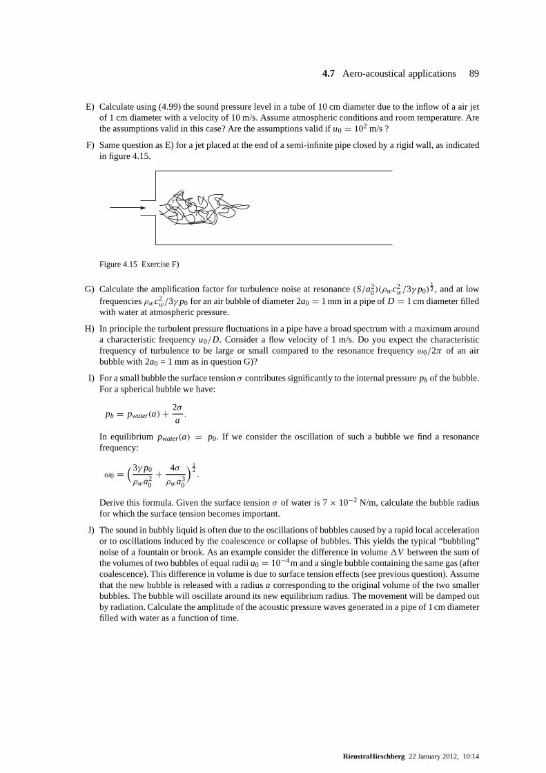
4.7 Aero-acoustical applications 89
E) Calculate using (4.99) the sound pressure level in a tube of 10 cm diameter due to the inflow of a air jetof 1 cm diameter with a velocity of 10 m/s. Assume atmosphericconditions and room temperature. Arethe assumptions valid in this case? Are the assumptions valid if u0 = 102 m/s ?
F) Same question as E) for a jet placed at the end of a semi-infinite pipe closed by a rigid wall, as indicatedin figure 4.15.
Figure 4.15 Exercise F)
G) Calculate the amplification factor for turbulence noise at resonance(S/a20)(ρwc2
w/3γ p0)12 , and at low
frequenciesρwc2w/3γ p0 for an air bubble of diameter 2a0 = 1 mm in a pipe ofD = 1 cm diameter filled
with water at atmospheric pressure.
H) In principle the turbulent pressure fluctuations in a pipehave a broad spectrum with a maximum arounda characteristic frequencyu0/D. Consider a flow velocity of 1 m/s. Do you expect the characteristicfrequency of turbulence to be large or small compared to the resonance frequencyω0/2π of an airbubble with 2a0 = 1 mm as in question G)?
I) For a small bubble the surface tensionσ contributes significantly to the internal pressurepb of the bubble.For a spherical bubble we have:
pb = pwater(a)+2σ
a.
In equilibrium pwater(a) = p0. If we consider the oscillation of such a bubble we find a resonancefrequency:
ω0 =(3γ p0
ρwa20
+ 4σ
ρwa30
) 12.
Derive this formula. Given the surface tensionσ of water is 7× 10⁻² N/m, calculate the bubble radiusfor which the surface tension becomes important.
J) The sound in bubbly liquid is often due to the oscillationsof bubbles caused by a rapid local accelerationor to oscillations induced by the coalescence or collapse ofbubbles. This yields the typical “bubbling”noise of a fountain or brook. As an example consider the difference in volume1V between the sum ofthe volumes of two bubbles of equal radiia0 = 10−4m and a single bubble containing the same gas (aftercoalescence). This difference in volume is due to surface tension effects (see previous question). Assumethat the new bubble is released with a radiusa corresponding to the original volume of the two smallerbubbles. The bubble will oscillate around its new equilibrium radius. The movement will be damped outby radiation. Calculate the amplitude of the acoustic pressure waves generated in a pipe of 1cm diameterfilled with water as a function of time.
RienstraHirschberg 22 January 2012, 10:14

5 Resonators and self-sustained oscillations
5.1 Self-sustained oscillations, shear layers and jets
When using Lighthill’s analogy to estimate the intensity ofthe sound produced by a turbulent flowin section 4.7.1 we have assumed that the sound source is independent of the acoustic field. Thisassumption was not justified but it seems reasonable if the acoustic velocities in the flow are “smallenough”. In fact this hypothesis breaks down in a large number of very interesting cases. In manyof these cases the acoustic feedback (influence of the sound field on the sound source) results in theoccurrence of a sharply defined harmonic oscillation, due tothe instability of the flow. Whistling,jet-screech and reheat-buzz are examples of such oscillations. In general the maintenance of suchoscillations implies the existence of a feedback loop as shown in figure 5.1.
edge hydrodynamicinstability
acousticresonator
hydrodynamic feedback
acoustic feedback
Figure 5.1 Flow-acoustic oscillator.
In most cases the acoustic field interacts with an intrinsically unstable hydrodynamic flow (jet, shearlayer) at a sharp edge where the flow separates from the wall. This separation point appears to be alocalized region where the acoustic flow and the hydrodynamic flow are strongly coupled. We willnow consider this interaction in some detail.
1234567123456712345671234567123456712345671234567
−∂p
∂r
ρv2
r
v
Figure 5.2 Flow in a bend.
In principle, if the flow were frictionless and is described accuratelyby a potential flow, the velocity at an edge would be infinitelylarge.This can be understood by considering the flow in a pipe at a bend(figure 5.2).
The fluid particles passing the bend feel a centrifugal forceρu2ϑ/r per
unit volume. If the flow is stationary it is obvious that thereshould bea centripetal force compensating the centrifugal force. Ina frictionlessflow the only force available is the pressure gradient−∂p/∂r . Hence,we see that the pressure at the outer wall in the bend should belargerthan at the inner wall. Using the equation of Bernoulli for a stationaryincompressible flow(p + 1
2ρv2 = constant) we conclude that the
velocity is larger at the inner wall than at the outer wall! (See figure 5.3.)
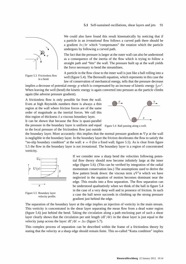
5.1 Self-sustained oscillations, shear layers and jets 91
rv
Figure 5.3 Frictionless flowin a bend.
We could also have found this result kinematically by noticing that ifa particle in anirrotational flow follows a curved path there should bea gradient∂v/∂r which “compensates” the rotation which the particleundergoes by following a curved path.
The fact that the pressure is larger at the outer wall can alsobe understoodas a consequence of the inertia of the flow which is trying to follow astraight path and “hits” the wall. The pressure built up at the wall yieldsthe force necessary to bend the streamlines.
A particle in the flow close to the inner wall is just like a ballrolling into awell (figure 5.4). The Bernoulli equation, which representsin this case thelaw of conservation of mechanical energy, tells that the pressure decrease
implies a decrease of potential energyp which is compensated by an increase of kinetic energy12ρv
2.When leaving the well (bend) the kinetic energy is again converted into pressure as the particle climbsagain (the adverse pressure gradient).
v v
v
Figure 5.4 Ball passing along a well.
A frictionless flow is only possible far from the wall.Even at high Reynolds numbers there is always a thinregion at the wall where friction forces are of the sameorder of magnitude as the inertial forces. We call thisthin region of thicknessδ a viscous boundary layer.It can be shown that because the flow is quasi-parallelthe pressure in the boundary layer is uniform and equalto the local pressure of the frictionless flow just outsidethe boundary layer. More accurately: this implies that the normal pressure gradientn·∇ p at the wallis negligible in the boundary layer. In the boundary layer the friction decelerates the flow to satisfy the“no-slip boundary condition” at the wall:v = 0 (for a fixed wall; figure 5.5). As is clear from figure5.5 the flow in the boundary layer is not irrotational. The boundary layer is a region of concentratedvorticity.
123456789012345678901234567890121234567890123456789012345678901234567890123456789012345678901212345678901234567890123456789012345678901234567890123456789012123456789012345678901234567890123456789012345678901234567890121234567890123456789012345678901234567890123456789012345678901212345678901234567890123456789012345678901234567890123456789012123456789012345678901234567890
U0
U (y)δ
x
y
Figure 5.5 Boundary layervelocity profile.
If we consider now a sharp bend the velocities following poten-tial flow theory should now become infinitely large at the inneredge (figure 5.6). (This can be verified by integration of the radialmomentum conservation law.) The assumptions used to derivetheflow pattern break down: the viscous termη∇2v which we haveneglected in the equation of motion becomes dominant near theedge. This results into a flow separation. The flow separationcanbe understood qualitatively when we think of the ball in figure 5.4in the case of a very deep well and in presence of friction. In sucha case the ball never succeeds in climbing up the strong pressuregradient just behind the edge.
The separation of the boundary layer at the edge implies an injection of vorticity in the main stream.This vorticity is concentrated in the shear layer separating the mean flow from a dead water region(figure 5.6) just behind the bend. Taking the circulation along a path enclosing part of such a shearlayer clearly shows that the circulation per unit length(d0/d`) in the shear layer is just equal to thevelocity jump across the layer: d0/d` = 1v (figure 5.7).
This complex process of separation can be described within the frame of a frictionless theory bystating that the velocity at a sharp edge should remain finite. This so-called “Kutta condition” implies
RienstraHirschberg 22 January 2012, 10:14

92 5 Resonators and self-sustained oscillations
1234567890123456789012345612345678901234567890123456123456789012345678901234561234567890123456789012345612345678901234567890123456123456789012345678901234561234567890123456789012345612345678901234567890123456123456789012345678901234561234567890123456789012345612345678901234567890123456123456789012345678901234561234567890123456789012345612345678901234567890123456123456789012345678901234561234567890123456789012345612345678901234567890123456123456789012345678901234561234567890123456789012345612345678901234567890123456123456789012345678901234561234567890123456789012345612345678901234567890123456123456789012345678901234561234567890123456789012345612345678901234567890123456
123456789012345678901234567890123456789012345678901234567890123456789012345678901234567890123456789012345678901234567890123456789012345678901234567890123456789012345678901234567890123456789012345678901234567890123456789012345678901234567890123456789012345678901234567890123456789012345678901234567890123456789012345678901234567890123456789012345678901234567890123456789012345678901234567890123456789012345678901234567890123456789012345678901234567890123456789012345678901234567890123456789012345678901234567890123456789012345678901234567890123456789012345678901234567890123456789012345678901234567890123456789012345678901234567890123456789012345678901234567890123456789012345678901234567890123456789012345678901234567890123456789012345678901234567890123456789012345678901234567890
1234567890123456789012345678901212345678901234123456789012345678901234567890121234567890123412345678901234567890123456789012123456789012341234567890123456789012345678901212345678901234123456789012345678901234567890121234567890123412345678901234567890123456789012123456789012341234567890123456789012345678901212345678901234123456789012345678901234567890121234567890123412345678901234567890123456789012123456789012341234567890123456789012345678901212345678901234123456789012345678901234567890121234567890123412345678901234567890123456789012123456789012341234567890123456789012345678901212345678901234123456789012345678901234567890121234567890123412345678901234567890123456789012123456789012341234567890123456789012345678901212345678901234123456789012345678901234567890121234567890123412345678901234567890123456789012123456789012341234567890123456789012345678901212345678901234123456789012345678901234567890121234567890123412345678901234567890123456789012123456789012341234567890123456789012345678901212345678901234123456789012345678901234567890121234567890123412345678901234567890123456789012123456789012341234567890123456789012345678901212345678901234123456789012345678901234567890121234567890123412345678901234567890123456789012123456789012341234567890123456789012345678901212345678901234123456789012345678901234567890121234567890123412345678901234567890123456789012123456789012341234567890123456789012345678901212345678901234123456789012345678901234567890121234567890123412345678901234567890123456789012123456789012341234567890123456789012345678901212345678901234123456789012345678901234567890121234567890123412345678901234567890123456789012123456789012341234567890123456789012345678901212345678901234123456789012345678901234567890121234567890123412345678901234567890123456789012123456789012341234567890123456789012345678901212345678901234123456789012345678901234567890121234567890123412345678901234567890123456789012123456789012341234567890123456789012345678901212345678901234123456789012345678901234567890121234567890123412345678901234567890123456789012123456789012341234567890123456789012345678901212345678901234
12345678901234567890123456789012123456789012345678123456789012345678901234567890121234567890123456781234567890123456789012345678901212345678901234567812345678901234567890123456789012123456789012345678123456789012345678901234567890121234567890123456781234567890123456789012345678901212345678901234567812345678901234567890123456789012123456789012345678123456789012345678901234567890121234567890123456781234567890123456789012345678901212345678901234567812345678901234567890123456789012123456789012345678123456789012345678901234567890121234567890123456781234567890123456789012345678901212345678901234567812345678901234567890123456789012123456789012345678123456789012345678901234567890121234567890123456781234567890123456789012345678901212345678901234567812345678901234567890123456789012123456789012345678123456789012345678901234567890121234567890123456781234567890123456789012345678901212345678901234567812345678901234567890123456789012123456789012345678123456789012345678901234567890121234567890123456781234567890123456789012345678901212345678901234567812345678901234567890123456789012123456789012345678123456789012345678901234567890121234567890123456781234567890123456789012345678901212345678901234567812345678901234567890123456789012123456789012345678123456789012345678901234567890121234567890123456781234567890123456789012345678901212345678901234567812345678901234567890123456789012123456789012345678123456789012345678901234567890121234567890123456781234567890123456789012345678901212345678901234567812345678901234567890123456789012123456789012345678123456789012345678901234567890121234567890123456781234567890123456789012345678901212345678901234567812345678901234567890123456789012123456789012345678123456789012345678901234567890121234567890123456781234567890123456789012345678901212345678901234567812345678901234567890123456789012123456789012345678123456789012345678901234567890121234567890123456781234567890123456789012345678901212345678901234567812345678901234567890123456789012123456789012345678123456789012345678901234567890121234567890123456781234567890123456789012345678901212345678901234567812345678901234567890123456789012123456789012345678123456789012345678901234567890121234567890123456781234567890123456789012345678901212345678901234567812345678901234567890123456789012123456789012345678
a) b)
Figure 5.6 Sharp bend. a) potential flow; b) actual flow.
123456789012345678901234561234567890123456789012345612345678901234567890123456123456789012345678901234561234567890123456789012345612345678901234567890123456123456789012345678901234561234567890123456789012345612345678901234567890123456123456789012345678901234561234567890123456789012345612345678901234567890123456123456789012345678901234561234567890123456789012345612345678901234567890123456123456789012345678901234561234567890123456789012345612345678901234567890123456123456789012345678901234561234567890123456789012345612345678901234567890123456123456789012345678901234561234567890123456789012345612345678901234567890123456
>v = U0 ex
�
-?
6-�d`
v = 0
shear layer
d0 =∮v · ds = −U0d`
Figure 5.7 Circulation in the shear layer
that a thin shear layer should be shed at the edge. The shear layer contains a distribution of vorticitysuch that the velocity induced at the edge by the vorticity just compensates the singularity of thepotential flow (which would exist in absence of shear layer).
It can be shown that this condition also implies that the shear layer is shed tangentially to the wallat the side of the edge where the flow velocity is the largest. The validity of a Kutta condition foran unsteady flow has been the subject of quite a long controversy. At this moment for a sharp edgethis is an accepted principle. Hence if next to a stationary flow we impose an unsteady potential flow(acoustic perturbation) the amount of vorticity shed at theedge will be modulated because we modifythe singular potential flow at the edge.
We see therefore that within a potential flow theory the sharpedges play a crucial rôle because theyare locations at which a potential flow can generate vorticity.1 It is not surprising therefore that innature the feedback from the acoustic field on a flow will oftenbe concentrated at an edge.
Self-sustained oscillations imply an amplification of the acoustic perturbations of the main flow byflow instability (this is the energy supply in the feedback loop). The instability of a thin shear layercan be understood by considering as a model an infinitely longrow of line vortices in a 2-D flow(figure 5.8).
The velocity induced by a line vortex of strength0 is calculated using Biot-Savart’s law:
uϑ = 0
2πr, (5.1)
wherer is the distance between the point at which we consider the velocity and the vortex. As we seein figure 5.8a a row of vortices is (meta)stable because the velocity induced on a given vortex by the
1In a two dimensional frictionless incompressible flow Dω/Dt = 0 so that there is no interaction between the vorticaland potential flow which can changeω within the flow.
RienstraHirschberg 22 January 2012, 10:14

5.1 Self-sustained oscillations, shear layers and jets 93
0
0
v = 0
2π
( 1
1`+ 1
21`+ · · ·
)
1`
v = − 0
2π
( 1
1`+ 1
21`+ · · ·
)
v = 10
2π1`0′ +10
v = − 10
2π1`
Figure 5.8 Instability of a vortex row induced by a non-uniformity of d0/d`.
vortices left of the point are just compensated by the velocities induced by the vortices at the right (bysymmetry). This is, however, a metastable situation as any perturbation will induce a growing flowinstability. For example a lateral displacement of one of the vortices out of the row is sufficient. Hencewe understand (figure 5.8b) that a modulation of the vorticity by acoustic perturbations can induce aroll up of the shear layer into a vortex structure as shown in figure 5.9.
Figure 5.9 Shear layer instability.
The most unstable type of flows is the flow between two shear layers of opposite vorticity: jets andwakes (figure 5.10). A wake appears to be so unstable that whenfriction forces are sufficiently small(above a certain Reynolds number) it is absolutely unstable[88]. Hence, any perturbation will resultin a break up of the wake structure shown in figure 5.10. A typical result of this is the occurrence ofvortices, periodically shed from a cylinder forRe > 50, which is known as the Von Kármán vortexstreet [18]. This periodic vortex shedding is responsible for the typical whistle of an empty luggagegrid on a car. A jet left alone (free jet) will also exhibit some specific oscillations at moderate Reynoldsnumbers (Re = O(103)) [16]. Turbulence will, however, kill any clear structure at higher Reynoldsnumbers. A jet needs a little help to start whistling. However, there are many ways to persuade him towhistle!
RienstraHirschberg 22 January 2012, 10:14
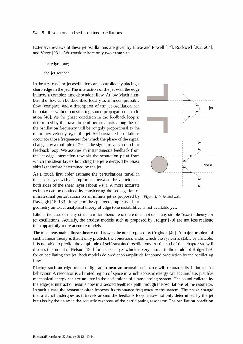
94 5 Resonators and self-sustained oscillations
Extensive reviews of these jet oscillations are given by Blake and Powell [17], Rockwell [202, 204],and Verge [231]. We consider here only two examples:
– the edge tone;
– the jet screech.
jet
wake
Figure 5.10 Jet and wake.
In the first case the jet oscillations are controlled by placing asharp edge in the jet. The interaction of the jet with the edgeinduces a complex time dependent flow. At low Mach num-bers the flow can be described locally as an incompressibleflow (compact) and a description of the jet oscillation canbe obtained without considering sound propagation or radi-ation [40]. As the phase condition in the feedback loop isdetermined by the travel time of perturbations along the jet,the oscillation frequency will be roughly proportional to themain flow velocityV0 in the jet. Self-sustained oscillationsoccur for those frequencies for which the phase of the signalchanges by a multiple of 2π as the signal travels around thefeedback loop. We assume an instantaneous feedback fromthe jet-edge interaction towards the separation point fromwhich the shear layers bounding the jet emerge. The phaseshift is therefore determined by the jet.
As a rough first order estimate the perturbations travel inthe shear layer with a compromise between the velocities atboth sides of the shear layer (about1
2V0). A more accurateestimate can be obtained by considering the propagation ofinfinitesimal perturbations on an infinite jet as proposed byRayleigh [16, 183]. In spite of the apparent simplicity of thegeometry an exact analytical theory of edge tone instabilities is not available yet.
Like in the case of many other familiar phenomena there does not exist any simple “exact” theory forjet oscillations. Actually, the crudest models such as proposed by Holger [79] are not less realisticthan apparently more accurate models.
The most reasonable linear theory until now is the one proposed by Crighton [40]. A major problem ofsuch a linear theory is that it only predicts the conditions under which the system is stable or unstable.It is not able to predict the amplitude of self-sustained oscillations. At the end of this chapter we willdiscuss the model of Nelson [156] for a shear-layer which is very similar to the model of Holger [79]for an oscillating free jet. Both models do predict an amplitude for sound production by the oscillatingflow.
Placing such an edge tone configuration near an acoustic resonator will dramatically influence itsbehaviour. A resonator is a limited region of space in which acoustic energy can accumulate, just likemechanical energy can accumulate in the oscillations of a mass-spring system. The sound radiated bythe edge-jet interaction results now in a second feedback path through the oscillations of the resonator.In such a case the resonator often imposes its resonance frequency to the system. The phase changethat a signal undergoes as it travels around the feedback loop is now not only determined by the jetbut also by the delay in the acoustic response of the participating resonator. The oscillation condition
RienstraHirschberg 22 January 2012, 10:14
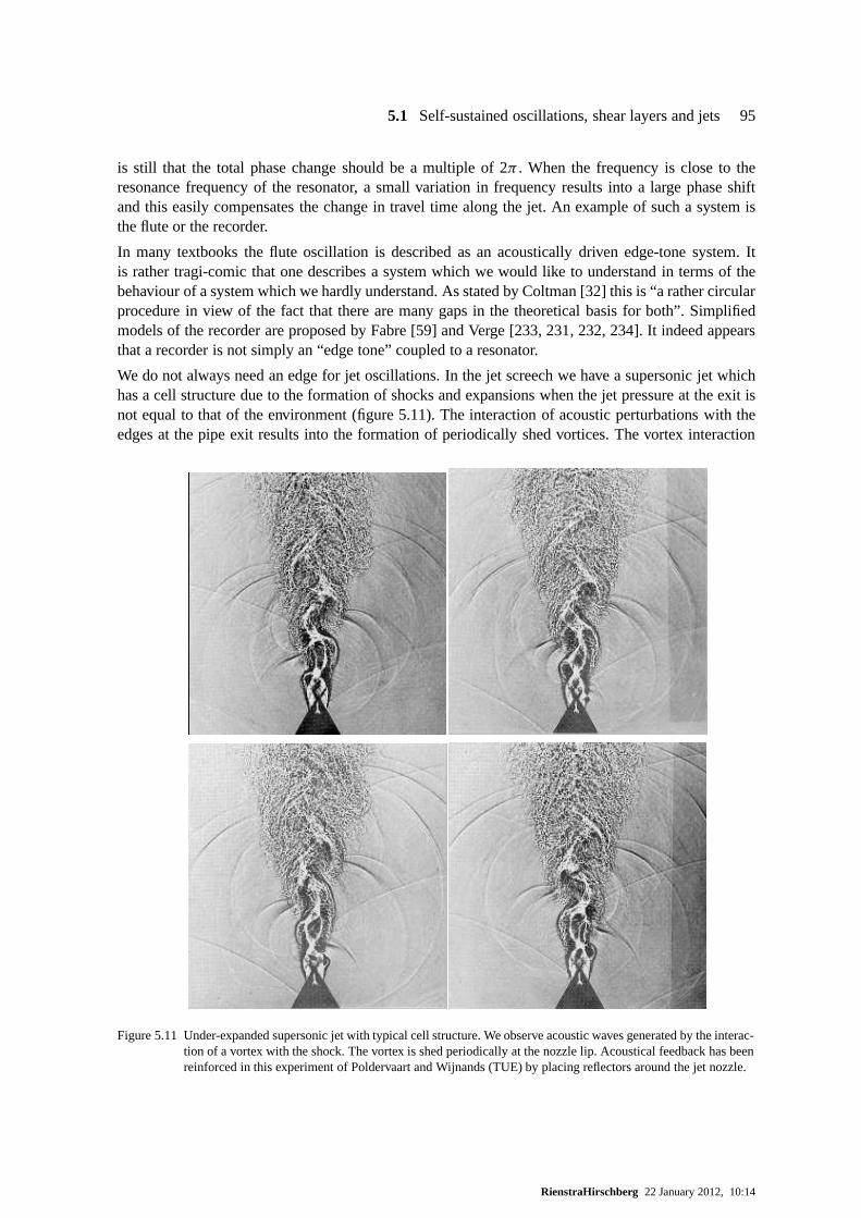
5.1 Self-sustained oscillations, shear layers and jets 95
is still that the total phase change should be a multiple of 2π . When the frequency is close to theresonance frequency of the resonator, a small variation in frequency results into a large phase shiftand this easily compensates the change in travel time along the jet. An example of such a system isthe flute or the recorder.
In many textbooks the flute oscillation is described as an acoustically driven edge-tone system. Itis rather tragi-comic that one describes a system which we would like to understand in terms of thebehaviour of a system which we hardly understand. As stated by Coltman [32] this is “a rather circularprocedure in view of the fact that there are many gaps in the theoretical basis for both”. Simplifiedmodels of the recorder are proposed by Fabre [59] and Verge [233, 231, 232, 234]. It indeed appearsthat a recorder is not simply an “edge tone” coupled to a resonator.
We do not always need an edge for jet oscillations. In the jet screech we have a supersonic jet whichhas a cell structure due to the formation of shocks and expansions when the jet pressure at the exit isnot equal to that of the environment (figure 5.11). The interaction of acoustic perturbations with theedges at the pipe exit results into the formation of periodically shed vortices. The vortex interaction
Figure 5.11 Under-expanded supersonic jet with typical cell structure. We observe acoustic waves generated by the interac-tion of a vortex with the shock. The vortex is shed periodically at the nozzle lip. Acoustical feedback has beenreinforced in this experiment of Poldervaart and Wijnands (TUE) by placing reflectors around the jet nozzle.
RienstraHirschberg 22 January 2012, 10:14

96 5 Resonators and self-sustained oscillations
with a shock wave appears to generate strong acoustic pulses. In particular the interaction with thethird cell appears to result into a localized periodic source of sound. The acoustic wave travels backtowards the pipe exit via the quiescent environment of the jet. This feedback loop can be blockedby placing a wall of absorbing material around the jet [174, 204]. This reduces the jet oscillations,demonstrating that the feedback loop described is the one which controls the jet oscillations. A reviewof some related supersonic flow oscillations is given by Jungowski [101].
Many of the features observed in a jet oscillation can also beobserved in a shear layer separating auniform main flow from a dead water region in a cavity [203] (closed side branch in a pipe system oropen roof of a car). We will discuss these types of oscillations after we have discussed the acousticsof some elementary type of acoustic resonators.
5.2 Some resonators
5.2.1 Introduction
Before considering other types of acoustically controlledflow instabilities we will focus our attentionon the acoustic resonator. This is an essential step becausein many applications the identification ofthe resonator is sufficient to find a cure to self-sustained oscillations. Furthermore resonators are alsoused to impede the propagation of sound or to enhance absorption. An example of this behaviour isthe reflection of acoustic waves by an air bubble in a pipe filled with water (section 4.4.5). We startour discussion with explaining the occurrence of resonancein a duct segment. We then will discussthe behaviour of the Helmholtz resonator.
5.2.2 Resonance in duct segment
We will first discuss the behaviour of a pipe segment excited by an oscillating piston. The most effi-cient way to do this is to consider this behaviour in linear approximation for a harmonically oscillatingpiston. We will see at the end of this section that at criticalfrequencies the theory does not providea solution if we neglect friction. In the time domain we can understand this so-called resonance be-haviour more easily. For this reason we will start our discussion by considering the problem in thetime domain.
Consider a pipe segment 0< x < L closed atx = L by a rigid wall (u·n = 0) and atx = 0 by anoscillating piston with a velocityup(t):
up = upE(t) at x = 0 (5.2)
where, in order to simplify the notation, we introduced in this subsection the auxiliary function
E(t) = H (t)eiωt . (5.3)
We assume thatup/c0 � 1 so that an acoustic approximation is valid. We consider only plane waves(ωA1/2/c0 � 1) and we neglect friction and heat transfer ((ν/ωA)1/2 � 1). The piston starts oscil-lating att = 0 and we assume that initially the fluid in the pipe is quiescent and uniform (u0 = 0). Insuch a case at least for short times the linear (acoustic) approximation is valid. We can now calculatethe acoustic field by using the method of characteristics as described in section 4.2. We will describe
RienstraHirschberg 22 January 2012, 10:14

5.2 Some resonators 97
t
x
I
II
III
IV
V
VI
t=x/c0
t=(2L−x)/c0
t=(2L+x)/c0
t=(4L−x)/c0
t=(4L+x)/c0
Figure 5.12 Wave pattern induced by a moving piston atx = 0, starting att = 0.
the calculation in detail. However, a reader only interested in the final result can jump to the finalresult, equation (5.16). The(x, t) diagram is shown in figure 5.12.
In region I we have a quiescent fluid:
pI = 0 and uI = 0. (5.4)
In region II we have thec+ waves generated at the piston:
pII = p+II
(t − x
c0
). (5.5)
Using the boundary conditionuII = up for x = 0 we find:
p+II (t) = ρ0c0up(t) = ρ0c0upE(t). (5.6)
In region III we have a superposition of thec+ waves emanating from region II and thec− wavesgenerated at the wallx = L:
pIII = p+II
(t − x
c0
)+ p−
III
(t + x − L
c0
). (5.7)
p−III can be determined by application of the boundary conditionuIII = 0 atx = L:
upE(t − L
c0
)− 1
ρ0c0p−
III (t) = 0. (5.8)
Hence we have:
pIII = ρ0c0up
{E
(t − x
c0
)+ E
(t + x − 2L
c0
)}. (5.9)
In region IV we have a superposition of thec− waves from region III and thec+ waves generated atthe pistonx = 0:
pIV = p−III
(t + x − L
c0
)+ p+
IV
(t − x
c0
). (5.10)
RienstraHirschberg 22 January 2012, 10:14

98 5 Resonators and self-sustained oscillations
p+IV is determined by applying the boundary conditionuIV = up at x = 0:
upE(t − 2L
c0
)− 1
ρ0c0p+
IV (t) = upE(t) (5.11)
and so we find:
pIV = ρ0c0up
{E
(t − x
c0
)+ E
(t + x − 2L
c0
)+ E
(t − x + 2L
c0
)}. (5.12)
In region V we have thec+ waves from region IV superimposed on thec− waves generated at the wallx = L:
pV = p+IV
(t − x
c0
)+ p−
V
(t + x − L
c0
). (5.13)
As before,p−V is determined by applying the boundary conditionuV = 0 atx = L. We find:
pV = ρ0c0up
{E
(t − x
c0
)+ E
(t + x − 2L
c0
)+ E
(t − x + 2L
c0
)+ E
(t + x − 4L
c0
)}. (5.14)
If we now limit ourselves to the positionx = 0 we see that after each period of time 2L/c0 a newwave is added to the original waves reflected at the wall and piston. These original waves have nowan additional phase of 2kL, wherek = ω/c0.
Substitutingx = 0 in (5.13) and generalizing the structure of the formula we find for 2N L/c0 < t <2(N + 1)L/c0:
p2N = 2ρ0c0up eiωt
{N∑
n=0
e−2iknL H(t − 2nL
c0
)− 1
2
}. (5.15)
This structure could also have been obtained by using the method of images described in section 4.6.2.We consider the piston as a volume source placed atx = 0+. Placing image sources in an infinitelyextended tube atx = ±2nL/c0 and summing up all the waves generated yields:
p = ρ0c0upE(t − |x|
c0
)+ ρ0c0up
∞∑
n=1
{E
(t − |x − 2nL|
c0
)+ E
(t − |x + 2nL|
c0
)}. (5.16)
Note that this series contains always only a finite number of non-zero terms, because for largen theargument of the Heaviside function inE becomes negative. So we have (fort > 0)
p
ρ0c0upe−iωt = e−ikx
N1∑
n=0
e−2iknL + eikxN2∑
n=1
e−2iknL,
N1 =⌊c0t − x
2L
⌋, N2 =
⌊c0t + x
2L
⌋,
wherebqc denotes the integer part ofq. It may be verified that after substitution ofx = 0 in (5.16)we find (5.15), withN = bc0t/2Lc. The geometric series may be summed2, so we obtain:
p
ρ0c0upe−iωt =
e−ikx 1 − e−2ik(N1+1)L
1 − e−2ikL+ eikx−2ikL 1 − e−2ikN2L
1 − e−2ikLif kL 6= π`,
e−ikx(N1 + 1)+ eikx N2 if kL = π`,
(5.17)
2Note that:N∑
n=0
an =
1 − aN+1
1 − aif a 6= 1,
N + 1 if a = 1,
N∑
n=1
an =
a1 − aN
1 − aif a 6= 1,
N if a = 1.
RienstraHirschberg 22 January 2012, 10:14
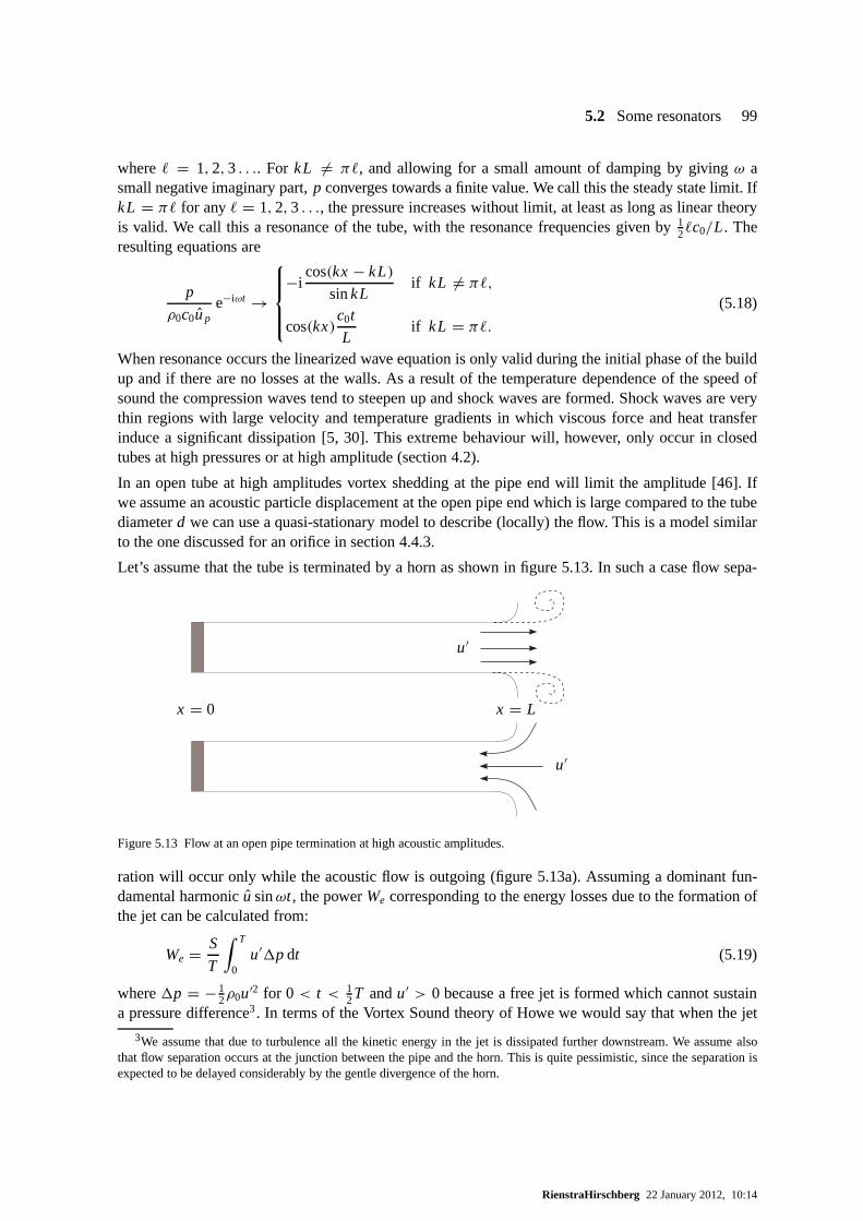
5.2 Some resonators 99
where` = 1,2,3 . . .. For kL 6= π`, and allowing for a small amount of damping by givingω asmall negative imaginary part,p converges towards a finite value. We call this the steady state limit. IfkL = π` for any` = 1,2,3 . . ., the pressure increases without limit, at least as long as linear theoryis valid. We call this a resonance of the tube, with the resonance frequencies given by12`c0/L. Theresulting equations are
p
ρ0c0upe−iωt →
−icos(kx − kL)
sinkLif kL 6= π`,
cos(kx)c0t
Lif kL = π`.
(5.18)
When resonance occurs the linearized wave equation is only valid during the initial phase of the buildup and if there are no losses at the walls. As a result of the temperature dependence of the speed ofsound the compression waves tend to steepen up and shock waves are formed. Shock waves are verythin regions with large velocity and temperature gradientsin which viscous force and heat transferinduce a significant dissipation [5, 30]. This extreme behaviour will, however, only occur in closedtubes at high pressures or at high amplitude (section 4.2).
In an open tube at high amplitudes vortex shedding at the pipeend will limit the amplitude [46]. Ifwe assume an acoustic particle displacement at the open pipeend which is large compared to the tubediameterd we can use a quasi-stationary model to describe (locally) the flow. This is a model similarto the one discussed for an orifice in section 4.4.3.
Let’s assume that the tube is terminated by a horn as shown in figure 5.13. In such a case flow sepa-
x = 0 x = L
u′
u′
Figure 5.13 Flow at an open pipe termination at high acousticamplitudes.
ration will occur only while the acoustic flow is outgoing (figure 5.13a). Assuming a dominant fun-damental harmonicu sinωt , the powerWe corresponding to the energy losses due to the formation ofthe jet can be calculated from:
We = S
T
∫ T
0u′1p dt (5.19)
where1p = −12ρ0u′2 for 0 < t < 1
2T andu′ > 0 because a free jet is formed which cannot sustaina pressure difference3. In terms of the Vortex Sound theory of Howe we would say that when the jet
3We assume that due to turbulence all the kinetic energy in thejet is dissipated further downstream. We assume alsothat flow separation occurs at the junction between the pipe and the horn. This is quite pessimistic, since the separationisexpected to be delayed considerably by the gentle divergence of the horn.
RienstraHirschberg 22 January 2012, 10:14

100 5 Resonators and self-sustained oscillations
is formed during the outflow there is a deviation from potential flow resulting intop′ = p′ex, while
potential flow theory would predictp′ = p′ex − 1
2ρ0u′2. This is due to the vorticity in the jet whichresults into a source of sound, that we can represent by a pressure source1p = −1
2ρ0u′2.
For 12T < t < T andu′ < 0 we have:
1p = 0 (5.20)
because we have a potential inflow into the pipe. Hence:
We ' −12ρ0u3S
T
∫ 12 T
0sin3ωt dt = − 1
3πρ0u
3S. (5.21)
The amplitude of the acoustic field in the tube can now be estimated by assuming that the lossesWe
at the open end balance the acoustic powerWp delivered by the piston:
Wp = S
T
∫ T
0up p′(x = 0)dt. (5.22)
Assuming that friction losses at the pipe wall are negligible we have:
Wp ' 12 Supρ0c0u, (5.23)
whereu is measured at the open pipe exit. Hence we find fromWe + Wp = 0:
u
c0=
√3π
2
up
c0. (5.24)
The model proposed here is valid when the Strouhal number based on the diameter and the acousticalvelocity is smaller than 1,i.e.ωd < u.
The non-linear behaviour of resonators, occurring for example with flow separation, makes such de-vices efficient sound absorbers. Sound is “caught” by the resonator and dissipated by vortex shedding.
In many cases the most significant losses are friction lossesat the wall. We will discuss the influence ofradiation from an open pipe end in section 6.7. When a plane wave approximation is valid a harmonicacoustic field in a pipe with uniform cross section can in the absence of mean flow still be describedby:
p′ = p+ eiωt−ikx +p− eiωt+ikx . (5.25)
The wave numberk, however, is now complex and is in first order approximation given by:
k = k0 + (1 − i )α (5.26)
wherek0 = ω/c0 andα is the damping coefficient given by equation (2.13), derivedin section 4.5.(In a liquid one should assumeγ ' 1.)
Damping also affects the impedanceZc of an infinite tube. To leading order approximation one finds[121]:
Zc = p′
u′ = ±Z0k0
k(5.27)
RienstraHirschberg 22 January 2012, 10:14
5.2 Some resonators 101
where the sign indicates the direction of the wave propagation (+x or −x) andZ0 = ρ0c0. We furthersee that wave speedc is affected:
c = c0Re(k)
k0(5.28)
While friction is relatively easily taken into account for harmonic waves, in the time domain frictioninvolves a convolution integral which makes the solution ofproblems more difficult to analyse [30].We will now further limit our discussion to the case of harmonic waves. Hence we seek only for asteady state solution and we assume that linear acoustics isvalid.
As an example we consider a piston with a velocityup = up eiωt at x = 0 exciting a tube of crosssectionS closed atx = L by a rigid wall. We neglect the radiation losses atx = L (which we willdiscuss further in section 6.7). The boundary conditions atx = 0 andx = L can be written in termsof equation (5.25) as:
up = p+ − p−
Zc(5.29)
and
0 = p+ e−ikL −p− eikL (5.30)
so that we find:
p+ = Zcup
1 − e−2ikL. (5.31)
In contrast to our earlier examplep+ does not become infinitely large with resonance becausek iscomplex. The impedanceZp seen by the piston atx = 0 is given by:
Zp = p+ + p−
up= −i Zc cotg(kL). (5.32)
Upon resonance, Re(k) = nπ/L with n = 1,2,3, ..., we find for the caseαL � 1:
Zp ' Zc
αL. (5.33)
When the damping(αL) predicted by laminar boundary layer theory is small the oscillation am-plitudes may become so large that the acoustical boundary layers become turbulent. This implies anon-linear energy dissipation as discussed in section 4.5.3.
5.2.3 The Helmholtz resonator (quiescent fluid)
The resonance conditions for a duct segment (5.25) imply that the tube length should be of the orderof magnitude of the acoustic wave length (kL = O(1)). In many technical applications this wouldimply that resonators used to absorb sound should be large (and expensive). A solution to this problemis to use a non-uniform pipe in the shape of a bottle. When the bottle is small compared to the acousticwave length (for low frequencies), the body of the bottle acts as an acoustic spring while the neck ofthe bottle is an acoustic mass (figure 5.14).
RienstraHirschberg 22 January 2012, 10:14

102 5 Resonators and self-sustained oscillations
SbV p′
in
u′in ' 0
u′n
`
p′ex
Sn
Km
Figure 5.14 Helmholtz resonator as mass-spring system.
If the cross-sectional areaSb of the bottle is large compared to the cross sectional areaSn of the neck,the acoustic velocities in the bottle will be small comparedto those in the neck. Hence we may infirst order approximation assume that the pressure and density perturbationsp′
in andρ ′in in the bottle
are uniform. Furthermore, as we have assumed the bottle neck(length`) to be acoustically compact,i.e. short compared to the wave length,k` � 1, we can neglect compressibility and integrate theline integral of the momentum equation along a streamline from a point inside to a point outside asfollows. Use identity (1.30) and the fact thatω×v is orthogonal to a streamline to obtain
ρ0
∫ ex
in
∂v′
∂t·ds + 1
2ρ0(u
′ex
2 − u′in
2)+ (p′ex − p′
in) =∫ ex
inµ∇v′ ·ds (5.34)
Assuming that the streamline does not change in time (for example the center streamline) we have∫ ex
in
∂v′
∂t·ds = d
dt
∫ ex
inv′ ·ds (5.35)
The velocity line integral evidently scales on a typical length times a typical velocity. If friction effectsare minor and the velocity is reasonably uniform, we can use the neck velocityu′
n with a correspondinglength being the neck length, added by a small end correctionδ (4.51) to take into account the inertiaof the acoustic flow at both ends just outside the neck (insideand outside the resonator); see section5.2.3.1. Then we have:
∫ ex
inv′ ·ds = (`+ 2δ)u′
n. (5.36)
The stress term line integral is far more difficult to assess.Apart fromu′n itself, it will depend on flow
profile, Reynolds number, wall heat exchange, turbulence, separation from sharp edges, and maybemore. For the moment we will take these effects together in a resistance factorR, which will a prioribe assumed to be relatively small, to have resonance and a small decay per period in the first place.
∫ ex
inµ∇v′ ·ds = −Ru′
n (5.37)
Due to separation from the outer exit, we have with outflowuin ' 0 with uex = u′n jetting out, while
similarly during inflow,uex ' 0 with uin = u′n jetting into the cavity. The pressure in the jets, however,
has to remain equal to the surrounding pressure (p′ex andp′
in respectively) because the boundary of thejet cannot support a pressure difference. Therefore, we have altogether
ρ0(`+ 2δ)d
dtu′
n + 1
2ρ0u
′n|u′
n| + Ru′n = p′
in − p′ex (5.38)
In order to have a second equation betweenp′n andu′
n we apply the integral mass conservation lawon the volumeV of the bottle. The change of mass must be equal to the flux through the bottle neck,
RienstraHirschberg 22 January 2012, 10:14
5.2 Some resonators 103
which is in linearised form for the density perturbationρ ′in:
Vdρ ′
in
dt= −ρu′
nSn ' −ρ0u′nSn. (5.39)
Assuming an adiabatic compression of the fluid in the bottle we can eliminateρ ′in by using the consti-
tutive equation:
p′in = c2
0ρ′in. (5.40)
Elimination ofρ ′in andu′
n from (5.38) by using (5.39) and (5.40) yields:
(`+ 2δ)V
c20Sn
d2 p′in
dt2+ V2
2ρ0c40S2
n
dp′in
dt
∣∣∣∣dp′
in
dt
∣∣∣∣ + RV
ρ0c20Sn
dp′in
dt+ p′
in = p′ex. (5.41)
When the damping is small, there exist solutions without external forcingp′ex, i.e. resonance solutions.
(`+ 2δ)V
c20Sn
d2 p′in
dt2+ p′
in = 0.
Hence we see that the Helmholtz resonator reacts as a mass-spring system with a resonance frequencyω0 given by:
ω20 = Snc2
0
(`+ 2δ)V. (5.42)
When the amplitude is small, the damping will in general be linear. For larger amplitudes the dampingwill be nonlinear, which among other things generates otherharmonics than the frequency of thedriving force; see section 5.2.4. A spectacular effect of additional damping occurs when the flow inthe neck is superimposed on a mean flow, forcing vortex shedding from the exit even without nonlinearterms; see section 5.2.5.
5.2.3.1 Intermezzo: End correction
If, as is the case in many technical applications, an orifice is used instead of bottle neck (` = 0), theuse of a reasonable estimate forδ is important. For an orifice with a circular aperture we have in thelimit of small k
δ = 0.85( Sn
π
) 12. (5.43)
For an unflanged thin-walled open-pipe end we can use for small k the approximation:
δ = 0.61( Sn
π
) 12. (5.44)
See also section 6.7. Values ofδ for various other geometries are given by Ingard [91].
RienstraHirschberg 22 January 2012, 10:14
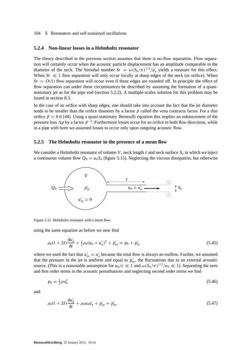
104 5 Resonators and self-sustained oscillations
5.2.4 Non-linear losses in a Helmholtz resonator
The theory described in the previous section assumes that there is no-flow separation. Flow separa-tion will certainly occur when the acoustic particle displacement has an amplitude comparable to thediameter of the neck. The Strouhal numberSr = ω(Sn/π)
1/2/u′n yields a measure for this effect.
WhenSr � 1 flow separation will only occur locally at sharp edges of theneck (or orifice). WhenSr = O(1) flow separation will occur even if these edges are rounded off. In principle the effect offlow separation can under these circumstances be described by assuming the formation of a quasi-stationary jet as for the pipe end (section 5.2.2). A multiple-scales solution for this problem may befound in section 8.3.
In the case of an orifice with sharp edges, one should take intoaccount the fact that the jet diametertends to be smaller than the orifice diameter by a factorβ called the vena contracta factor. For a thinorifice β ' 0.6 [44]. Using a quasi-stationary Bernoulli equation this implies an enhancement of thepressure loss1p by a factorβ−2. Furthermore losses occur for an orifice in both flow directions, whilein a pipe with horn we assumed losses to occur only upon outgoing acoustic flow.
5.2.5 The Helmholtz resonator in the presence of a mean flow
We consider a Helmholtz resonator of volumeV , neck length and neck surfaceSn in which we injecta continuous volume flowQ0 = u0Sn (figure 5.15). Neglecting the viscous dissipation, but otherwise
Q0
V
p′in
u′in ' 0
`
u0 + u′n Sn
Figure 5.15 Helmholtz resonator with a mean flow.
using the same equation as before we now find
ρ0(`+ 2δ)du′
n
dt+ 1
2ρ0(u0 + u′n)
2 + p′ex = p0 + p′
in (5.45)
where we used the fact thatu′ex = u′
n because the total flow is always an outflow. Further, we assumedthat the pressure in the jet is uniform and equal top′
ex, the fluctuations due to an external acousticsource. (This is a reasonable assumption foru0/c � 1 andω(Sn/π)
1/2/u0 � 1). Separating the zeroand first order terms in the acoustic perturbations and neglecting second order terms we find
p0 = 12ρu2
0 (5.46)
and
ρ0(`+ 2δ)du′
n
dt+ ρ0u0u′
n + p′ex = p′
in. (5.47)
RienstraHirschberg 22 January 2012, 10:14

5.3 Green’s function of a finite duct 105
Using the linearized mass conservation law we have neglecting terms of order(u0/c0)2:
Vdρ ′
in
dt= −(ρ0u
′n + ρ ′
exu0)Sn. (5.48)
Eliminating ρ ′in by using the constitutive equationp′
in = c20ρ
′in and eliminatingp′
in from (5.47) and(5.48) we find:
d2u′n
dt2+ u0
`+ 2δ
du′n
dt+ ω2
0un = −ω20M0
ρ0c0p′
ex − 1
ρ0(`+ 2δ)
dp′ex
dt.
ω0 is defined by equation (5.42) andM0 = u0/c0. For a harmonic excitationp′ex = pexeiωt we find:
ρ0c0un
pex= − M0 + iω1ω/ω
20
1 − (ω/ω0)2 + i M0ω1ω/ω20
(5.49)
whereω1 = c0/(`+2δ). We see that the mean flow induces a damping factor which we might a priorinot have expected because we did not assume friction losses nor heat transfer.
The key assumption which has introduced damping is that we have assumed that the pressure pertur-bation at the pipe exit is equal to the environment pressure perturbationpex. This is true, because theflow leaves the exit as a jet4, which implies separation of the flow at the pipe exit and a Kutta conditionto be added to an inviscid model (section 5.1)! This implies that a varying exit velocityun modulatesthe vorticity shed at the edges of the pipe exit, which is, on its turn, a loss of kinetic energy for theacoustic field. This confirms that the Kutta condition is indeed a quite significant assumption [39].
5.3 Green’s function of a finite duct
Formally, the Green’s function of a finite duct can be obtained if we neglect friction and losses at thepipe terminations by using the method of images (section 4.6.2 and section 5.2.2). For a pipe segment0 < x < L closed by rigid walls a source atx = y in the pipe segment is represented by a row ofsources (in an infinitely long pipe) at positions given by (figure 5.16)
xn = ±(2n + 1)L ± y; n = 0,1,2,3, ... (5.50)
The Green’s function is the sum of all the contributions of these sources:
Figure 5.16 Images of source atx = y.
4A very interesting proof of the fact that a quasi-stationarysubsonic free jet cannot sustain any pressure difference withthe environment is provided by Shapiro [217].
RienstraHirschberg 22 January 2012, 10:14

106 5 Resonators and self-sustained oscillations
g(x, t|y, τ ) = 1
2c0
∞∑
n=0
{H
(t − τ + x + (2n + 1)L − y
c0
)
+ H(t − τ + x + (2n + 1)L + y
c0
)
+ H(t − τ − x − (2n + 1)L − y
c0
)
+ H(t − τ − x − (2n + 1)L + y
c0
)}. (5.51)
It is clear that such a formal solution has no simple physicalinterpretation.
Another representation for the 1-D Green’s function on[0, L] that might be useful in some applica-tions is found by a series expansion of the Fourier transformg of g:
g =∞∑
n=0
An fn(x) (5.52)
in a suitable basis{ fn}. In this case we willnot start from elementary solutions of the wave equation.The functionsfn we will consider will (only) satisfy the boundary conditions atx = 0 andx = L, sothat their sum will automatically satisfy these conditionsif this sum converges uniformly. Hence wewill construct now atailoredGreen’s function (section 3.1). Furthermore, it is evidently necessary thatthe basis{ fn} is complete, and convenient that it is orthogonal to some suitable inner product. Let’snow for simplicity assume that the pipe segment is limited bya rigid wall atx = 0 and an impedanceZL at x = L. Consider:
fn = sin(Knx) (5.53)
with Kn determined by the equation
tan(Y)
Y= i
ZL
kL(5.54)
with KnL = Y. Note that forn → ∞ (ZL 6= 0)
KnL ' (n + 12)π + ikL
(n + 12)πZL
+ ... (5.55)
so that for largen, fn approaches the Fourier-sine series basis. The number of solutions between 0 and(n+ 1
2)π (for n → ∞) is not always exactlyn. Depending onZL/kL it may differ by 1. For example,if ZL/kL = i C andC is real, there is no purely imaginary solutionY = iσ with tanh(σ )/σ = −C ifC > 0 or C < −1, and exactly one solution if−1 < C < 0, which disappears to infinity ifC → 0.Finally, we note that{ fn} is orthogonal to theL2 inner product:
( fn, fm) =∫ L
0fn(x) fm(x)dx. (5.56)
(Note:not .. f ∗m(x) ..), which is easily seen by direct integration:
If n 6= m:∫ L
0sin(Knx) sin(Kmx)dx = sin(KnL − KmL)
2(Kn − Km)− sin(KnL + KmL)
2(Kn + Km)= 0 (5.57)
RienstraHirschberg 22 January 2012, 10:14

5.4 Self-sustained oscillations of a clarinet 107
after application of (5.54).If n = m:
∫ L
0sin2(Knx)dx = 1
2 L − sin(2KnL)
4Kn= 3n. (5.58)
We now seek an expression for the Green’s function, defined by:
d2g
dx2+ k2g = −δ(x − y)
c20
(5.59)
in the form (5.52). Substitution of the series, multiplication left- and right-hand side byfm, and inte-grating over[0, L] yields (because of orthogonality):
(k2 − K 2m)3mAm = − fm(y)/c
20. (5.60)
Hence we have:
g(x, y) = 1
c20
∞∑
n=0
fn(x) fn(y)
(K 2n − k2)3n
. (5.61)
We see explicitly that:
i) the Green’s function is indeed symmetric inx and y (source and observation points) as statedearlier in section 3.1 (reciprocity), and
ii) any source with a frequencyω = Kn c0 (so thatKn = k) yields an infinite field, in otherwords: resonance. Note that in generalKn is complex, so that such a source strength increasesexponentially in time.
When the frequencyω of the source is close to a resonance frequency this resonance will dominate theresponse of the pipe segment and we can use a single mode approximation of the Green’s function.This is the approximation which we will use when discussing the thermo-acoustic oscillations in apipe segment (Rijke tube, section 5.5).
5.4 Self-sustained oscillations of a clarinet
5.4.1 Introduction
The coupling of acoustic oscillations to mechanical vibrations is a technically important problem[240]. In some case such a coupling can cause the failure of a security valve. Instead of looking ata technical application we are going to consider a musical instrument. The model used is very crudeand only aims at illustrating the principles of two methods of analysis:
– the stability analysis;
– the temporal simulation.
In the first case we consider a linear model and deduce the minimal blowing pressure necessary toobtain self-sustained oscillations. In the second case we consider a simplified non-linear model de-veloped by McIntyreet al. [129] which can be used for time domain simulation. The aim ofthesimplification is to allow for a real time simulation of a clarinet! We will restrict our discussion to theprinciple of the solution of the problem. The results of the calculations can be found in the literature.
RienstraHirschberg 22 January 2012, 10:14
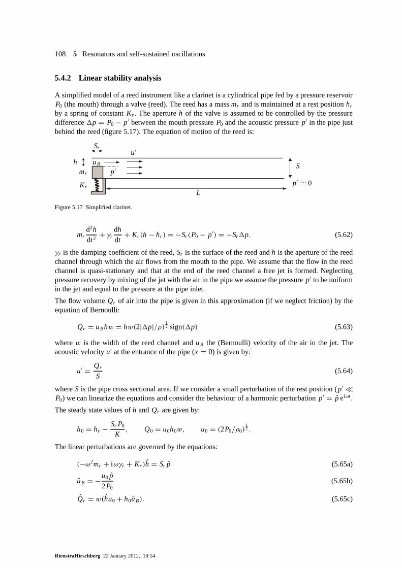
108 5 Resonators and self-sustained oscillations
5.4.2 Linear stability analysis
A simplified model of a reed instrument like a clarinet is a cylindrical pipe fed by a pressure reservoirP0 (the mouth) through a valve (reed). The reed has a massmr and is maintained at a rest positionhr
by a spring of constantKr . The apertureh of the valve is assumed to be controlled by the pressuredifference1p = P0 − p′ between the mouth pressureP0 and the acoustic pressurep′ in the pipe justbehind the reed (figure 5.17). The equation of motion of the reed is:
h uB
mr
Kr
Sr
p′
u′
L
S
p′ ' 0
Figure 5.17 Simplified clarinet.
mrd2h
dt2+ γr
dh
dt+ Kr (h − hr ) = −Sr (P0 − p′) = −Sr1p. (5.62)
γr is the damping coefficient of the reed,Sr is the surface of the reed andh is the aperture of the reedchannel through which the air flows from the mouth to the pipe.We assume that the flow in the reedchannel is quasi-stationary and that at the end of the reed channel a free jet is formed. Neglectingpressure recovery by mixing of the jet with the air in the pipewe assume the pressurep′ to be uniformin the jet and equal to the pressure at the pipe inlet.
The flow volumeQr of air into the pipe is given in this approximation (if we neglect friction) by theequation of Bernoulli:
Qr = uBhw = hw(2|1p|/ρ) 12 sign(1p) (5.63)
wherew is the width of the reed channel anduB the (Bernoulli) velocity of the air in the jet. Theacoustic velocityu′ at the entrance of the pipe (x = 0) is given by:
u′ = Qr
S(5.64)
whereS is the pipe cross sectional area. If we consider a small perturbation of the rest position (p′ �P0) we can linearize the equations and consider the behaviour of a harmonic perturbationp′ = p eiωt .
The steady state values ofh andQr are given by:
h0 = hr − Sr P0
K, Q0 = u0h0w, u0 = (2P0/ρ0)
12 .
The linear perturbations are governed by the equations:
(−ω2mr + iωγr + Kr )h = Sr p (5.65a)
uB = −u0 p
2P0(5.65b)
Qr = w(hu0 + h0uB). (5.65c)
RienstraHirschberg 22 January 2012, 10:14
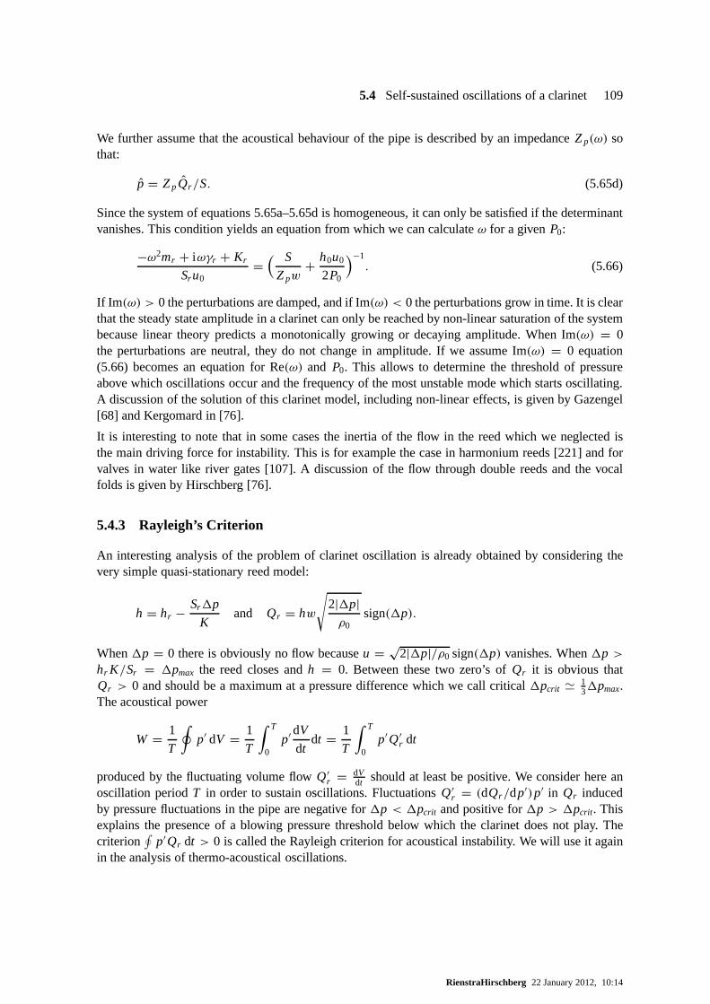
5.4 Self-sustained oscillations of a clarinet 109
We further assume that the acoustical behaviour of the pipe is described by an impedanceZp(ω) sothat:
p = ZpQr /S. (5.65d)
Since the system of equations 5.65a–5.65d is homogeneous, it can only be satisfied if the determinantvanishes. This condition yields an equation from which we can calculateω for a givenP0:
−ω2mr + iωγr + Kr
Sr u0=
( S
Zpw+ h0u0
2P0
)−1. (5.66)
If Im (ω) > 0 the perturbations are damped, and if Im(ω) < 0 the perturbations grow in time. It is clearthat the steady state amplitude in a clarinet can only be reached by non-linear saturation of the systembecause linear theory predicts a monotonically growing or decaying amplitude. When Im(ω) = 0the perturbations are neutral, they do not change in amplitude. If we assume Im(ω) = 0 equation(5.66) becomes an equation for Re(ω) and P0. This allows to determine the threshold of pressureabove which oscillations occur and the frequency of the mostunstable mode which starts oscillating.A discussion of the solution of this clarinet model, including non-linear effects, is given by Gazengel[68] and Kergomard in [76].
It is interesting to note that in some cases the inertia of theflow in the reed which we neglected isthe main driving force for instability. This is for example the case in harmonium reeds [221] and forvalves in water like river gates [107]. A discussion of the flow through double reeds and the vocalfolds is given by Hirschberg [76].
5.4.3 Rayleigh’s Criterion
An interesting analysis of the problem of clarinet oscillation is already obtained by considering thevery simple quasi-stationary reed model:
h = hr − Sr1p
Kand Qr = hw
√2|1p|ρ0
sign(1p).
When1p = 0 there is obviously no flow becauseu =√
2|1p|/ρ0 sign(1p) vanishes. When1p >hr K/Sr = 1pmax the reed closes andh = 0. Between these two zero’s ofQr it is obvious thatQr > 0 and should be a maximum at a pressure difference which we call critical 1pcrit ' 1
31pmax.The acoustical power
W = 1
T
∮p′ dV = 1
T
∫ T
0p′ dV
dtdt = 1
T
∫ T
0p′Q′
r dt
produced by the fluctuating volume flowQ′r = dV
dt should at least be positive. We consider here anoscillation periodT in order to sustain oscillations. FluctuationsQ′
r = (dQr /dp′)p′ in Qr inducedby pressure fluctuations in the pipe are negative for1p < 1pcrit and positive for1p > 1pcrit . Thisexplains the presence of a blowing pressure threshold belowwhich the clarinet does not play. Thecriterion
∮p′Qr dt > 0 is called the Rayleigh criterion for acoustical instability. We will use it again
in the analysis of thermo-acoustical oscillations.
RienstraHirschberg 22 January 2012, 10:14

110 5 Resonators and self-sustained oscillations
5.4.4 Time domain simulation
Early attempts to describe the non-linearity of a clarinet were based on a modal expansion of theacoustic field in the pipe. This implies that the Green’s function was approximated by taking thecontribution of a few (one to three) modes5 into account (equation (5.61)). The typical procedure isfurther to assume a weak non-linearity which implies that a perturbation method like the method ofaveraging can be used to calculate the time dependence of themodes [67]. A full solution is obtainedby the method of harmonic balance discussed by Gilbert [69].
As stated by McIntyre [129] the non-linearity in a clarinet is not weak. In fact the most spectacularnon-linearity is due to the limited movement of the reed uponclosing. The collision of the reed againstthe wall of the mouthpiece can result in a chaotic behaviour [68]. The key feature of a clarinet mouth-piece is that this abrupt non-linearity is replaced by a softer non-linearity because upon touching thewall the reed gradually closes as it is bent on the curved wallof the mouthpiece (called the lay) andits stiffness increases because the oscillating part is becoming shorter.
However, the high resonance frequency of the reedω2r = Kr /mr suggests that a quasi-stationary
model of the reed could be a fair first approximation. Hence McIntyre [129] proposes to use thesteady approximation of (5.62):
Kr (h − hr ) = −Sr (P0 − p′) = −Sr1p (5.67)
combined with (5.63), (5.64) and (5.65d). The numerical procedure is further based on the knowledgethat the acoustic pressurep′ at the reed is composed of an outgoing wavep+ and an incoming wavep− (result of the reflection of earlierp+ wave at the pipe end):
p′ = p+ + p−. (5.68)
The pipe has a characteristic impedanceZc (= ρ0c0 when friction is neglected) so that:
u′ = p+ − p−
Zc. (5.69)
If we now define the reflection functionr (t) as the acoustic wavep− induced by a pressure pulsep+ = δ(t), we find:
p− = r ∗ p+ (5.70)
where∗ indicates a convolution (equation C.10). Elimination ofp+ andp− from (5.68)–(5.70) yields:
p′ = Zcu′ + r ∗(Zcu
′ + p′) (5.71)
whereu′ is calculated at each time step by using (5.63), (5.66), and (5.67):
u′ = w
S
(hr − Sr1p
Kr
)(2|1p|ρ0
) 12
sign(1p). (5.72)
The solution is obtained by integrating (5.71) step by step,using the previous value ofp′ to calculateu′ in the convolution of the right-hand side (5.71).
5Standing waves in the pipe closed at the reed end.
RienstraHirschberg 22 January 2012, 10:14
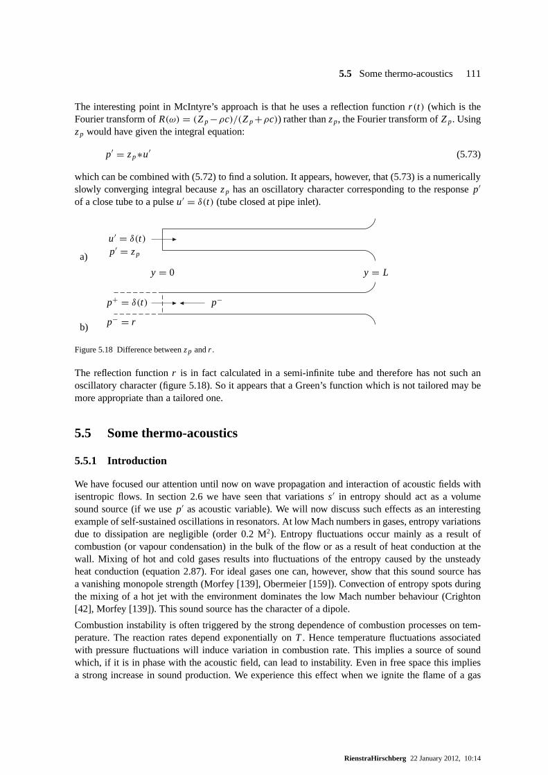
5.5 Some thermo-acoustics 111
The interesting point in McIntyre’s approach is that he usesa reflection functionr (t) (which is theFourier transform ofR(ω) = (Zp−ρc)/(Zp+ρc)) rather thanzp, the Fourier transform ofZp. Usingzp would have given the integral equation:
p′ = zp∗u′ (5.73)
which can be combined with (5.72) to find a solution. It appears, however, that (5.73) is a numericallyslowly converging integral becausezp has an oscillatory character corresponding to the responsep′
of a close tube to a pulseu′ = δ(t) (tube closed at pipe inlet).
u′ = δ(t)p′ = zp
p+ = δ(t) p−
p− = r
a)
b)
y = 0 y = L
Figure 5.18 Difference betweenzp andr .
The reflection functionr is in fact calculated in a semi-infinite tube and therefore has not such anoscillatory character (figure 5.18). So it appears that a Green’s function which is not tailored may bemore appropriate than a tailored one.
5.5 Some thermo-acoustics
5.5.1 Introduction
We have focused our attention until now on wave propagation and interaction of acoustic fields withisentropic flows. In section 2.6 we have seen that variationss′ in entropy should act as a volumesound source (if we usep′ as acoustic variable). We will now discuss such effects as aninterestingexample of self-sustained oscillations in resonators. At low Mach numbers in gases, entropy variationsdue to dissipation are negligible (order 0.2 M2). Entropy fluctuations occur mainly as a result ofcombustion (or vapour condensation) in the bulk of the flow oras a result of heat conduction at thewall. Mixing of hot and cold gases results into fluctuations of the entropy caused by the unsteadyheat conduction (equation 2.87). For ideal gases one can, however, show that this sound source hasa vanishing monopole strength (Morfey [139], Obermeier [159]). Convection of entropy spots duringthe mixing of a hot jet with the environment dominates the lowMach number behaviour (Crighton[42], Morfey [139]). This sound source has the character of adipole.
Combustion instability is often triggered by the strong dependence of combustion processes on tem-perature. The reaction rates depend exponentially onT . Hence temperature fluctuations associatedwith pressure fluctuations will induce variation in combustion rate. This implies a source of soundwhich, if it is in phase with the acoustic field, can lead to instability. Even in free space this impliesa strong increase in sound production. We experience this effect when we ignite the flame of a gas
RienstraHirschberg 22 January 2012, 10:14
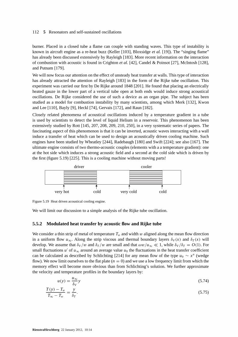
112 5 Resonators and self-sustained oscillations
burner. Placed in a closed tube a flame can couple with standing waves. This type of instability isknown in aircraft engine as a re-heat buzz (Keller [103], Bloxsidgeet al. [19]). The “singing flame”has already been discussed extensively by Rayleigh [183]. More recent information on the interactionof combustion with acoustic is found in Crightonet al. [42], Candel & Poinsot [27], McIntosh [128],and Putnam [179].
We will now focus our attention on the effect of unsteady heattransfer at walls. This type of interactionhas already attracted the attention of Rayleigh [183] in theform of the Rijke tube oscillation. Thisexperiment was carried our first by De Rijke around 1848 [201]. He found that placing an electricallyheated gauze in the lower part of a vertical tube open at both ends would induce strong acousticaloscillations. De Rijke considered the use of such a device asan organ pipe. The subject has beenstudied as a model for combustion instability by many scientists, among which Merk [132], Kwonand Lee [110], Bayly [9], Heckl [74], Gervais [172], and Raun[182].
Closely related phenomena of acoustical oscillations induced by a temperature gradient in a tubeis used by scientists to detect the level of liquid Helium in areservoir. This phenomenon has beenextensively studied by Rott [145, 207, 208, 209, 210, 250], in a very systematic series of papers. Thefascinating aspect of this phenomenon is that it can be inverted, acoustic waves interacting with a wallinduce a transfer of heat which can be used to design an acoustically driven cooling machine. Suchengines have been studied by Wheatley [244], Radebaugh [180] and Swift [224]; see also [167]. Theultimate engine consists of two thermo-acoustic couples (elements with a a temperature gradient): oneat the hot side which induces a strong acoustic field and a second at the cold side which is driven bythe first (figure 5.19) [225]. This is a cooling machine without moving parts!
driver cooler
very hot cold very cold cold
Figure 5.19 Heat driven acoustical cooling engine.
We will limit our discussion to a simple analysis of the Rijketube oscillation.
5.5.2 Modulated heat transfer by acoustic flow and Rijke tube
We consider a thin strip of metal of temperatureTw and widthw aligned along the mean flow directionin a uniform flow u∞. Along the strip viscous and thermal boundary layersδV(x) and δT (x) willdevelop. We assume thatδV/w andδT/w are small and thatωw/u∞ � 1, while δV/δT = O(1). Forsmall fluctuationsu′ of u∞ around an average valueu0 the fluctuations in the heat transfer coefficientcan be calculated as described by Schlichting [214] for any mean flow of the typeu0 ∼ xn (wedgeflow). We now limit ourselves to the flat plate (n = 0) and we use a low frequency limit from which thememory effect will become more obvious than from Schlichting’s solution. We further approximatethe velocity and temperature profiles in the boundary layersby:
u(y) = u∞δV
y (5.74)
T(y)− TwT∞ − Tw
= y
δT. (5.75)
RienstraHirschberg 22 January 2012, 10:14

5.5 Some thermo-acoustics 113
Such an approximation is only valid for low frequencies and small perturbation amplitudes, corre-sponding toωw/u∞ � 1 andu′/u0 � 1. Outside the boundary layers the flow is uniform. In thisapproximation the viscous stressτw at the wall is given by:
τw = ηu∞δV
(5.76)
and the heat transferq at the wall by:
q = −K(∂T
∂y
)y=0
= −KT∞ − TwδT
. (5.77)
Using an integral formulation of the conservation law in boundary layer approximation we find [214]:
[ ∂∂t
+ 1
3u∞
∂
∂x
]δ2
V = 4ν − 2δ2V
u∞
∂u∞∂t
(5.78a)
[ ∂∂t
+ 2
3u∞
( δT
δV
) ∂∂x
]δ2
T = 4a + 1
3u∞
( δT
δV
)3 ∂
∂xδ2
V for δT < δV (5.78b)
[ ∂∂t
+ u∞(1 −
( δT
δV
)2) ∂∂x
]δ2
T = 4a − u∞(2
3− δT
δV
) ∂∂xδ2
V for δT > δV (5.78c)
wherea is the thermal diffusivity of the gas:
a = K
ρCP. (5.79)
Note that we have used the assumption(Tw − T∞)/T∞ � 1 in order to keep the equations simple.This is certainly a very crude approximation in a Rijke tube.The boundary conditions are:
δV(0) = δT (0) = 0 atx = 0. (5.80)
In air we havePr < 1 and hence in generalδV < δT . We will, however, use further the assumptionPr = 1 because we do not expect an essentially different physicalbehaviour.
The stationary solution of (5.78a) is:
δV =(12νx
u0
) 12
(5.81)
while δT can be calculated from (5.78b):
δT = δV . (5.82)
Using the notationδ0 = δT = δV for the stationary solution we find in linear approximation:
[ ∂∂t
+ 1
3u0∂
∂x
]δ′
V = − δ0
u0
∂u′
∂t− 1
3u0
(δ′V
δ0+ u′
u0
)∂δ0
∂x(5.83a)
[ ∂∂t
+ 2
3u0∂
∂x
]δ′
T = +1
3u0∂δ′
V
∂x+ 1
3u0
(δ′V − δ′
T
δ0− u′
u0
)∂δ0
∂x, (5.83b)
RienstraHirschberg 22 January 2012, 10:14
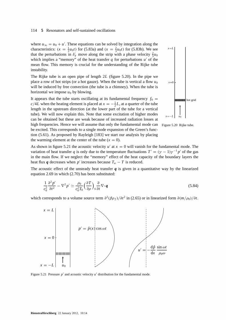
114 5 Resonators and self-sustained oscillations
hot grid
x=L
x=0
x=−L u0
6
Figure 5.20 Rijke tube.
whereu∞ = u0 + u′. These equations can be solved by integration along thecharacteristics:(x = 1
3u0t) for (5.83a) and(x = 23u0t) for (5.83b). We see
that the perturbations inδ′T move along the strip with a phase velocity2
3u0
which implies a “memory” of the heat transferq for perturbationsu′ of themean flow. This memory is crucial for the understanding of theRijke tubeinstability.
The Rijke tube is an open pipe of length 2L (figure 5.20). In the pipe weplace a row of hot strips (or a hot gauze). When the tube is vertical a flowu0
will be induced by free convection (the tube is a chimney). When the tube ishorizontal we imposeu0 by blowing.
It appears that the tube starts oscillating at its fundamental frequency f0 =c/4L when the heating element is placed atx = −1
2 L, at a quarter of the tubelength in the upstream direction (at the lower part of the tube for a verticaltube). We will now explain this. Note that some excitation ofhigher modescan be obtained but these are weak because of increased radiation losses athigh frequencies. Hence we will assume that only the fundamental mode canbe excited. This corresponds to a single mode expansion of the Green’s func-tion (5.61). As proposed by Rayleigh [183] we start our analysis by placingthe warming element at the center of the tube (x = 0).
As shown in figure 5.21 the acoustic velocityu′ at x = 0 will vanish for the fundamental mode. Thevariation of heat transferq is only due to the temperature fluctuationsT ′ = (γ − 1)γ −1 p′ of the gasin the main flow. If we neglect the “memory” effect of the heat capacity of the boundary layers theheat fluxq decreases whenp′ increases becauseTw − T is reduced.
The acoustic effect of the unsteady heat transferq is given in a quantitative way by the linearizedequation 2.69 in which (2.70) has been substituted:
1
c20
∂2 p′
∂t2− ∇2 p′ ' ρ0
c20T0
(∂T
∂ρ
)S
∂
∂t∇·q (5.84)
which corresponds to a volume source term∂2(βρ f )/∂t2 in (2.65) or in linearized form∂(m/ρ0)/∂t .
x = L
x = 0
x = −L u0
p′ = p(x) cosωt
u′ = −dp
dx
sinωt
ρ0ω
Figure 5.21 Pressurep′ and acoustic velocityu′ distribution for the fundamental mode.
RienstraHirschberg 22 January 2012, 10:14
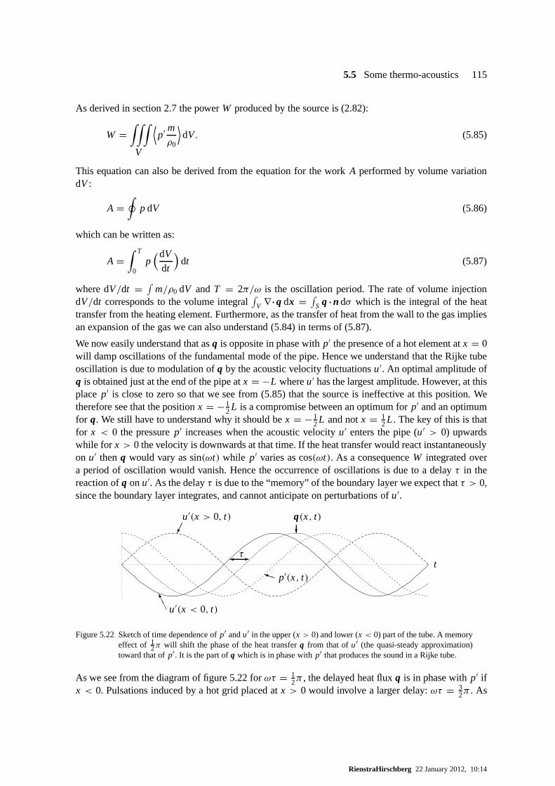
5.5 Some thermo-acoustics 115
As derived in section 2.7 the powerW produced by the source is (2.82):
W =∫∫∫
V
⟨p′ m
ρ0
⟩dV. (5.85)
This equation can also be derived from the equation for the work A performed by volume variationdV :
A =∮
p dV (5.86)
which can be written as:
A =∫ T
0p
(dV
dt
)dt (5.87)
where dV/dt =∫
m/ρ0 dV andT = 2π/ω is the oscillation period. The rate of volume injectiondV/dt corresponds to the volume integral
∫V ∇·q dx =
∫S q ·n dσ which is the integral of the heat
transfer from the heating element. Furthermore, as the transfer of heat from the wall to the gas impliesan expansion of the gas we can also understand (5.84) in termsof (5.87).
We now easily understand that asq is opposite in phase withp′ the presence of a hot element atx = 0will damp oscillations of the fundamental mode of the pipe. Hence we understand that the Rijke tubeoscillation is due to modulation ofq by the acoustic velocity fluctuationsu′. An optimal amplitude ofq is obtained just at the end of the pipe atx = −L whereu′ has the largest amplitude. However, at thisplacep′ is close to zero so that we see from (5.85) that the source is ineffective at this position. Wetherefore see that the positionx = −1
2 L is a compromise between an optimum forp′ and an optimumfor q. We still have to understand why it should bex = −1
2 L and notx = 12 L. The key of this is that
for x < 0 the pressurep′ increases when the acoustic velocityu′ enters the pipe (u′ > 0) upwardswhile for x > 0 the velocity is downwards at that time. If the heat transferwould react instantaneouslyon u′ thenq would vary as sin(ωt) while p′ varies as cos(ωt). As a consequenceW integrated overa period of oscillation would vanish. Hence the occurrence of oscillations is due to a delayτ in thereaction ofq onu′. As the delayτ is due to the “memory” of the boundary layer we expect thatτ > 0,since the boundary layer integrates, and cannot anticipateon perturbations ofu′.
u′(x > 0, t)���
q(x, t)?
u′(x < 0, t)AAK
τ�-
p′(x, t)PPit
Figure 5.22 Sketch of time dependence ofp′ andu′ in the upper (x > 0) and lower (x < 0) part of the tube. A memoryeffect of 1
2π will shift the phase of the heat transferq from that ofu′ (the quasi-steady approximation)toward that ofp′. It is the part ofq which is in phase withp′ that produces the sound in a Rijke tube.
As we see from the diagram of figure 5.22 forωτ = 12π , the delayed heat fluxq is in phase withp′ if
x < 0. Pulsations induced by a hot grid placed atx > 0 would involve a larger delay:ωτ = 32π . As
RienstraHirschberg 22 January 2012, 10:14
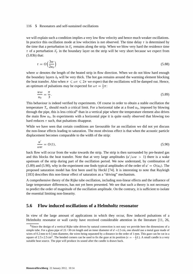
116 5 Resonators and self-sustained oscillations
we will explain such a condition implies a very low flow velocity and hence much weaker oscillations.In practice this oscillation mode at low velocities is not observed. The time delayτ is determined bythe time that a perturbation inδ′
T remains along the strip. When we blow very hard the residencetimeτ of a perturbationδ′
T in the boundary layer on the strip will be very short because we expect from(5.83b) that:
τ = O( 3w
2u0
)(5.88)
wherew denotes the length of the heated strip in flow direction. Whenwe do not blow hard enoughthe boundary layersδ0 will be very thick. The hot gas remains around the warming element blockingthe heat transfer. Also whenπ 6 ωτ 6 2π we expect that the oscillations will be damped out. Hence,an optimum of pulsations may be expected forωτ = 1
2π :
wω
u0= π
3. (5.89)
This behaviour is indeed verified by experiments. Of course in order to obtain a stable oscillation thetemperatureTw should reach a critical limit. For a horizontal tube at a fixedu0, imposed by blowingthrough the pipe, this is less critical6 than in a vertical pipe where the temperature element also drivesthe main flowu0. In experiments with a horizontal pipe it is quite easily observed that blowing toohard reducesτ such, that pulsations disappear.
While we have seen that certain conditions are favourable for an oscillation we did not yet discussthe non-linear effects leading to saturation. The most obvious effect is that when the acoustic particledisplacement becomes comparable to the width of the strip:
u′
ωw= O(1), (5.90)
back flow will occur from the wake towards the strip. The stripis then surrounded by pre-heated gasand this blocks the heat transfer. Note that at very large amplitudes (u′/ωw > 1) there is a wakeupstream of the strip during part of the oscillation period.We now understand, by combination of(5.89) and (5.90), why in the experiment one finds typical amplitudes of the order ofu′ = O(u0). Theproposed saturation model has first been used by Heckl [74]. It is interesting to note that Rayleigh[183] describes this non-linear effect of saturation as a “driving” mechanism.
A comprehensive theory of the Rijke tube oscillation, including non-linear effects and the influence oflarge temperature differences, has not yet been presented.We see that such a theory is not necessaryto predict the order of magnitude of the oscillation amplitude. On the contrary, it is sufficient to isolatethe essential limiting non-linearity.
5.6 Flow induced oscillations of a Helmholtz resonator
In view of the large amount of applications in which they occur, flow induced pulsations of aHelmholtz resonator or wall cavity have received considerable attention in the literature [11, 26,
6Since the design of a vertical Rijke tube driven by natural convection is not easy we provide here the dimensions of asimple tube. For a glass pipe of 2L=30 cm length and an inner diameter ofd =2.5 cm, one should use a metal gaze made ofwires of 0.2 mm to 0.5 mm diameter, the wires being separated by a distance in the order of 1 mm. This gaze can be cut in asquare of 2.5×2.5 cm2. The bended corners can be used to fix the gaze at its position (x = −1
2 L). A small candle is a verysuitable heat source. The pipe will produce its sound after the candle is drawn back.
RienstraHirschberg 22 January 2012, 10:14
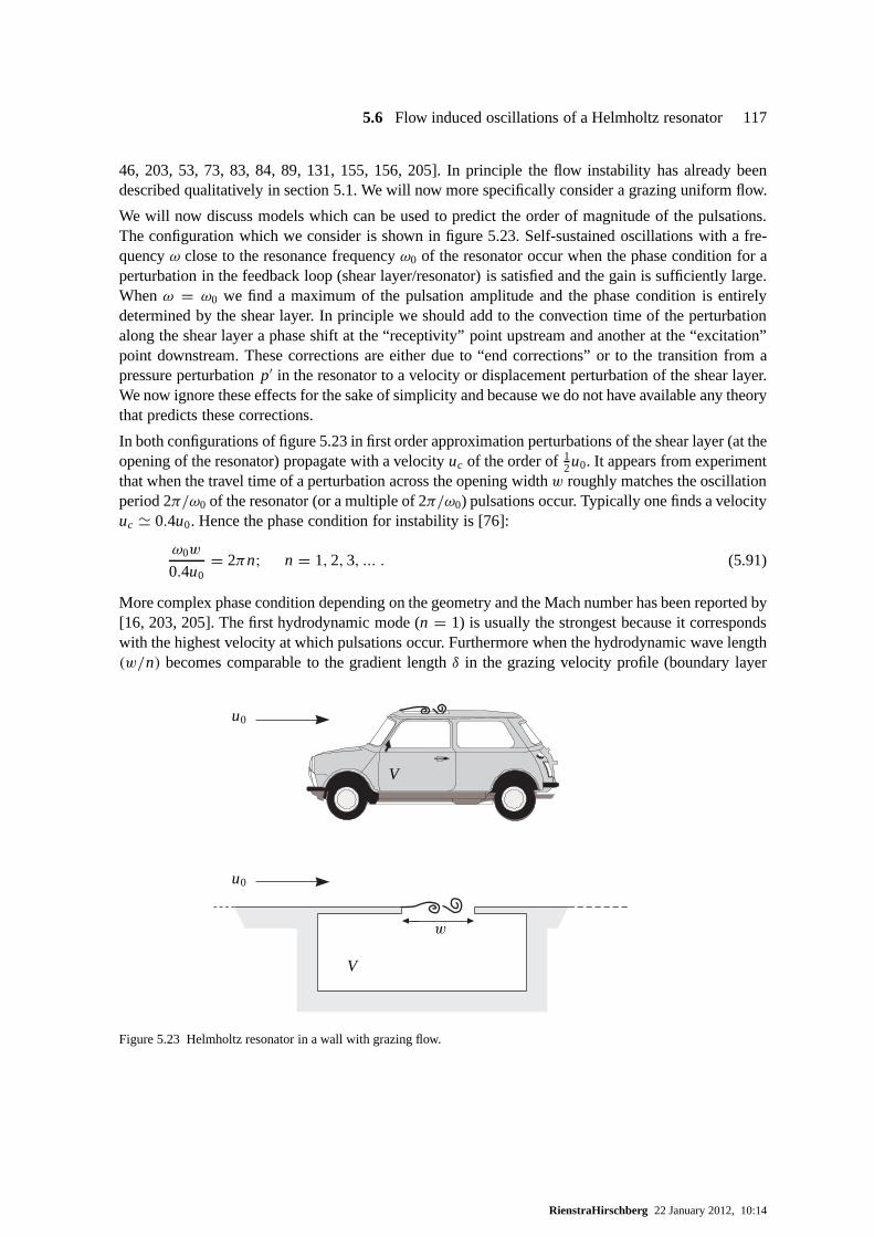
5.6 Flow induced oscillations of a Helmholtz resonator 117
46, 203, 53, 73, 83, 84, 89, 131, 155, 156, 205]. In principle the flow instability has already beendescribed qualitatively in section 5.1. We will now more specifically consider a grazing uniform flow.
We will now discuss models which can be used to predict the order of magnitude of the pulsations.The configuration which we consider is shown in figure 5.23. Self-sustained oscillations with a fre-quencyω close to the resonance frequencyω0 of the resonator occur when the phase condition for aperturbation in the feedback loop (shear layer/resonator)is satisfied and the gain is sufficiently large.Whenω = ω0 we find a maximum of the pulsation amplitude and the phase condition is entirelydetermined by the shear layer. In principle we should add to the convection time of the perturbationalong the shear layer a phase shift at the “receptivity” point upstream and another at the “excitation”point downstream. These corrections are either due to “end corrections” or to the transition from apressure perturbationp′ in the resonator to a velocity or displacement perturbationof the shear layer.We now ignore these effects for the sake of simplicity and because we do not have available any theorythat predicts these corrections.
In both configurations of figure 5.23 in first order approximation perturbations of the shear layer (at theopening of the resonator) propagate with a velocityuc of the order of12u0. It appears from experimentthat when the travel time of a perturbation across the opening widthw roughly matches the oscillationperiod 2π/ω0 of the resonator (or a multiple of 2π/ω0) pulsations occur. Typically one finds a velocityuc ' 0.4u0. Hence the phase condition for instability is [76]:
ω0w
0.4u0= 2πn; n = 1,2,3, ... . (5.91)
More complex phase condition depending on the geometry and the Mach number has been reported by[16, 203, 205]. The first hydrodynamic mode (n = 1) is usually the strongest because it correspondswith the highest velocity at which pulsations occur. Furthermore when the hydrodynamic wave length(w/n) becomes comparable to the gradient lengthδ in the grazing velocity profile (boundary layer
u0
u0
V
V
w
Figure 5.23 Helmholtz resonator in a wall with grazing flow.
RienstraHirschberg 22 January 2012, 10:14
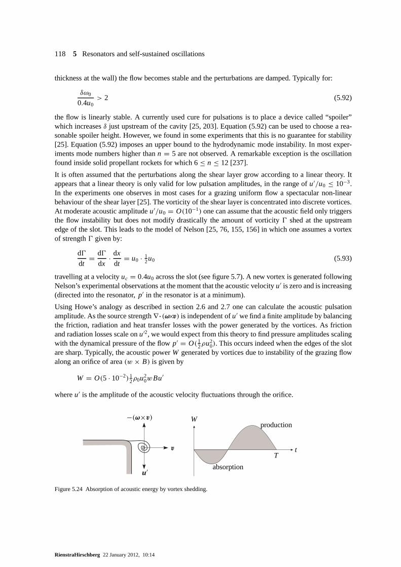
118 5 Resonators and self-sustained oscillations
thickness at the wall) the flow becomes stable and the perturbations are damped. Typically for:
δω0
0.4u0> 2 (5.92)
the flow is linearly stable. A currently used cure for pulsations is to place a device called “spoiler”which increasesδ just upstream of the cavity [25, 203]. Equation (5.92) can beused to choose a rea-sonable spoiler height. However, we found in some experiments that this is no guarantee for stability[25]. Equation (5.92) imposes an upper bound to the hydrodynamic mode instability. In most exper-iments mode numbers higher thann = 5 are not observed. A remarkable exception is the oscillationfound inside solid propellant rockets for which 6≤ n ≤ 12 [237].
It is often assumed that the perturbations along the shear layer grow according to a linear theory. Itappears that a linear theory is only valid for low pulsation amplitudes, in the range ofu′/u0 ≤ 10−3.In the experiments one observes in most cases for a grazing uniform flow a spectacular non-linearbehaviour of the shear layer [25]. The vorticity of the shearlayer is concentrated into discrete vortices.At moderate acoustic amplitudeu′/u0 = O(10−1) one can assume that the acoustic field only triggersthe flow instability but does not modify drastically the amount of vorticity 0 shed at the upstreamedge of the slot. This leads to the model of Nelson [25, 76, 155, 156] in which one assumes a vortexof strength0 given by:
d0
dt= d0
dx· dx
dt= u0 · 1
2u0 (5.93)
travelling at a velocityuc = 0.4u0 across the slot (see figure 5.7). A new vortex is generated followingNelson’s experimental observations at the moment that the acoustic velocityu′ is zero and is increasing(directed into the resonator,p′ in the resonator is at a minimum).
Using Howe’s analogy as described in section 2.6 and 2.7 one can calculate the acoustic pulsationamplitude. As the source strength∇·(ω×v) is independent ofu′ we find a finite amplitude by balancingthe friction, radiation and heat transfer losses with the power generated by the vortices. As frictionand radiation losses scale onu′2, we would expect from this theory to find pressure amplitudesscalingwith the dynamical pressure of the flowp′ = O(1
2ρu20). This occurs indeed when the edges of the slot
are sharp. Typically, the acoustic powerW generated by vortices due to instability of the grazing flowalong an orifice of area(w × B) is given by
W = O(5 · 10−2)12ρ0u2
0wBu′
whereu′ is the amplitude of the acoustic velocity fluctuations through the orifice.
−(ω×v)
v
u′
W
t
absorption
production
T
Figure 5.24 Absorption of acoustic energy by vortex shedding.
RienstraHirschberg 22 January 2012, 10:14
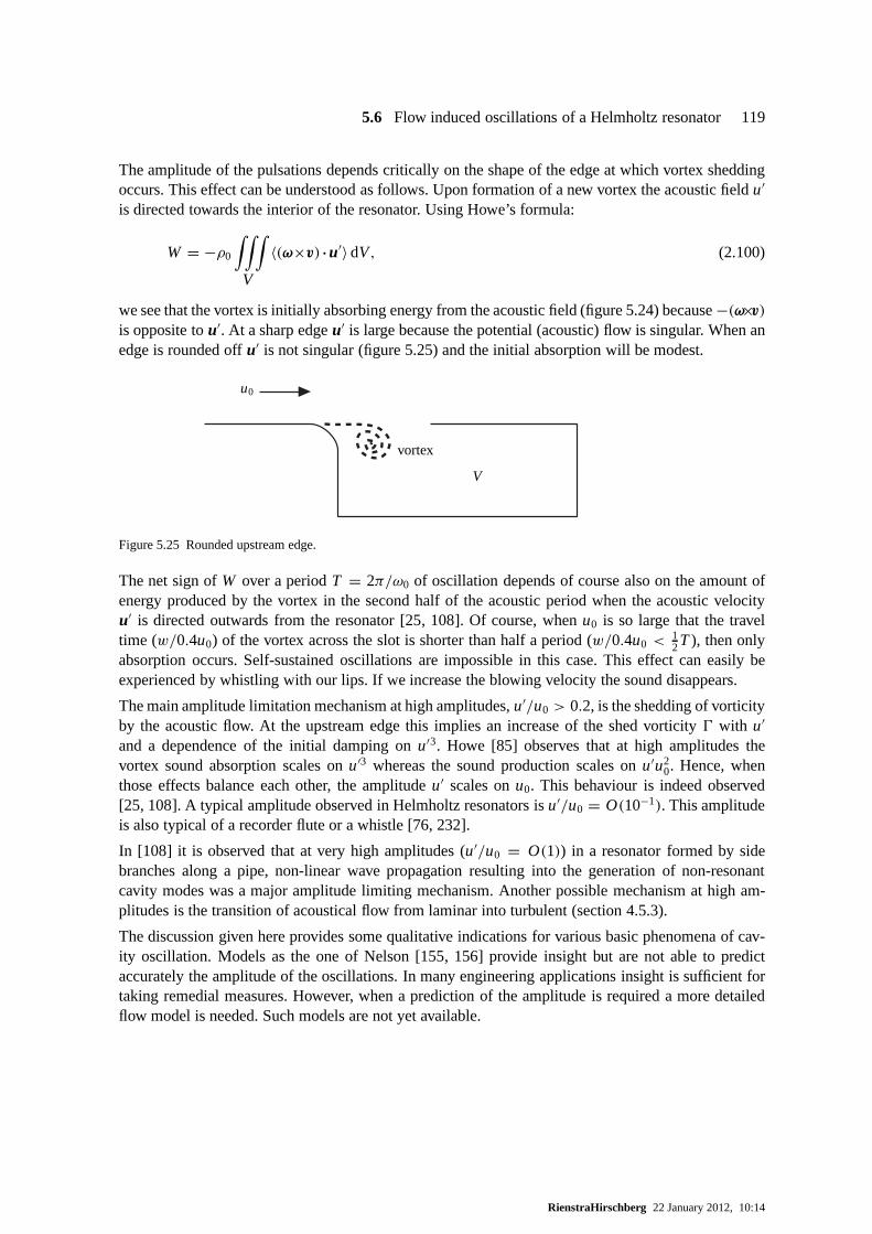
5.6 Flow induced oscillations of a Helmholtz resonator 119
The amplitude of the pulsations depends critically on the shape of the edge at which vortex sheddingoccurs. This effect can be understood as follows. Upon formation of a new vortex the acoustic fieldu′
is directed towards the interior of the resonator. Using Howe’s formula:
W = −ρ0
∫∫∫
V
〈(ω×v)·u′〉 dV, (2.100)
we see that the vortex is initially absorbing energy from theacoustic field (figure 5.24) because−(ω×v)is opposite tou′. At a sharp edgeu′ is large because the potential (acoustic) flow is singular. When anedge is rounded offu′ is not singular (figure 5.25) and the initial absorption willbe modest.
u0
vortex
V
Figure 5.25 Rounded upstream edge.
The net sign ofW over a periodT = 2π/ω0 of oscillation depends of course also on the amount ofenergy produced by the vortex in the second half of the acoustic period when the acoustic velocityu′ is directed outwards from the resonator [25, 108]. Of course, whenu0 is so large that the traveltime (w/0.4u0) of the vortex across the slot is shorter than half a period (w/0.4u0 <
12T), then only
absorption occurs. Self-sustained oscillations are impossible in this case. This effect can easily beexperienced by whistling with our lips. If we increase the blowing velocity the sound disappears.
The main amplitude limitation mechanism at high amplitudes, u′/u0 > 0.2, is the shedding of vorticityby the acoustic flow. At the upstream edge this implies an increase of the shed vorticity0 with u′
and a dependence of the initial damping onu′3. Howe [85] observes that at high amplitudes thevortex sound absorption scales onu′3 whereas the sound production scales onu′u2
0. Hence, whenthose effects balance each other, the amplitudeu′ scales onu0. This behaviour is indeed observed[25, 108]. A typical amplitude observed in Helmholtz resonators isu′/u0 = O(10−1). This amplitudeis also typical of a recorder flute or a whistle [76, 232].
In [108] it is observed that at very high amplitudes (u′/u0 = O(1)) in a resonator formed by sidebranches along a pipe, non-linear wave propagation resulting into the generation of non-resonantcavity modes was a major amplitude limiting mechanism. Another possible mechanism at high am-plitudes is the transition of acoustical flow from laminar into turbulent (section 4.5.3).
The discussion given here provides some qualitative indications for various basic phenomena of cav-ity oscillation. Models as the one of Nelson [155, 156] provide insight but are not able to predictaccurately the amplitude of the oscillations. In many engineering applications insight is sufficient fortaking remedial measures. However, when a prediction of theamplitude is required a more detailedflow model is needed. Such models are not yet available.
RienstraHirschberg 22 January 2012, 10:14
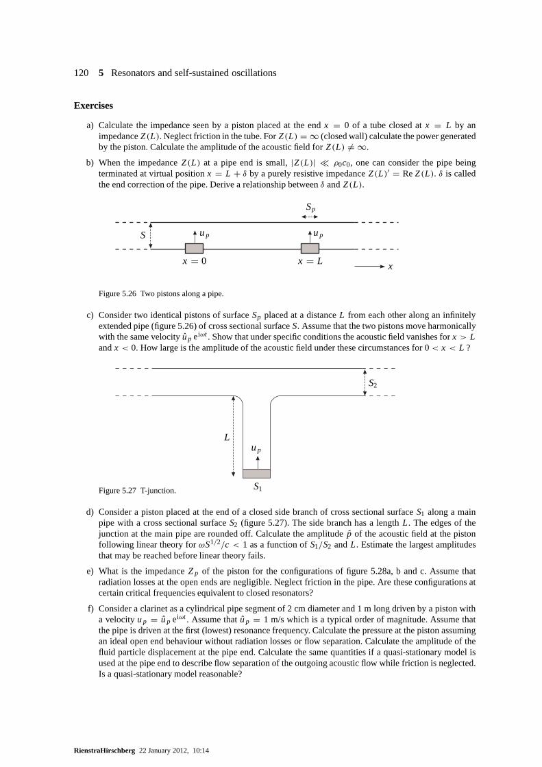
120 5 Resonators and self-sustained oscillations
Exercises
a) Calculate the impedance seen by a piston placed at the endx = 0 of a tube closed atx = L by animpedanceZ(L). Neglect friction in the tube. ForZ(L) = ∞ (closed wall) calculate the power generatedby the piston. Calculate the amplitude of the acoustic field for Z(L) 6= ∞.
b) When the impedanceZ(L) at a pipe end is small,|Z(L)| � ρ0c0, one can consider the pipe beingterminated at virtual positionx = L + δ by a purely resistive impedanceZ(L)′ = ReZ(L). δ is calledthe end correction of the pipe. Derive a relationship between δ andZ(L).
x = 0 x = L x
S up up
Sp
Figure 5.26 Two pistons along a pipe.
c) Consider two identical pistons of surfaceSp placed at a distanceL from each other along an infinitelyextended pipe (figure 5.26) of cross sectional surfaceS. Assume that the two pistons move harmonicallywith the same velocityup eiωt . Show that under specific conditions the acoustic field vanishes forx > Landx < 0. How large is the amplitude of the acoustic field under thesecircumstances for 0< x < L ?
S2
S1
up
L
Figure 5.27 T-junction.
d) Consider a piston placed at the end of a closed side branch of cross sectional surfaceS1 along a mainpipe with a cross sectional surfaceS2 (figure 5.27). The side branch has a lengthL. The edges of thejunction at the main pipe are rounded off. Calculate the amplitude p of the acoustic field at the pistonfollowing linear theory forωS1/2/c < 1 as a function ofS1/S2 andL. Estimate the largest amplitudesthat may be reached before linear theory fails.
e) What is the impedanceZp of the piston for the configurations of figure 5.28a, b and c. Assume thatradiation losses at the open ends are negligible. Neglect friction in the pipe. Are these configurations atcertain critical frequencies equivalent to closed resonators?
f) Consider a clarinet as a cylindrical pipe segment of 2 cm diameter and 1 m long driven by a piston witha velocityup = up eiωt . Assume thatup = 1 m/s which is a typical order of magnitude. Assume thatthe pipe is driven at the first (lowest) resonance frequency.Calculate the pressure at the piston assumingan ideal open end behaviour without radiation losses or flow separation. Calculate the amplitude of thefluid particle displacement at the pipe end. Calculate the same quantities if a quasi-stationary model isused at the pipe end to describe flow separation of the outgoing acoustic flow while friction is neglected.Is a quasi-stationary model reasonable?
RienstraHirschberg 22 January 2012, 10:14

5.6 Flow induced oscillations of a Helmholtz resonator 121
a)
p′ ' 0
L
S2
Lup
S1
©1
©2 ©3
b)
S S
S S
L2L
Lup
©1
©2 ©3
©4
©5
c)
p′ ' 0 p′ ' 0
L LS
Sup©1 ©2
Figure 5.28 Coupled T-junctions.
g) A pipe segment with a different cross sectional areaS2 than the cross sectionS1 of the rest of the pipecan be used as a filter to prevent the propagation of waves generated by a piston. Two solutions can beconsideredS2 > S1 andS1 < S2 (figure 5.29a and b). Assuming an ideal open end atx = L1 + L2 + L3,provide a set of equations from which we can calculate the amplitude of the acoustic velocityu endat thepipe end for a given velocityup of the piston.
h) Introduction:A possible 3-D model for a kettle drum consists of a cavity in free space, with acoustic perturbations
upp′ ' 0
L1 L2 L3
S1 S2 S1
upp′ ' 0S1 S2 S1
L1 L2 L3
Figure 5.29 Resonators in a pipe.
RienstraHirschberg 22 January 2012, 10:14
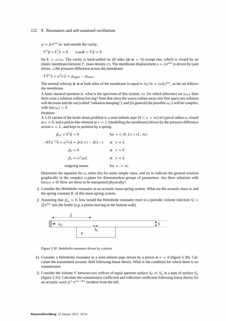
122 5 Resonators and self-sustained oscillations
p = peiωt in- and outside the cavity:
∇2 p + k2 p = 0, iωρ0u + ∇ p = 0
for k = ω/c0. The cavity is hard-walled on all sides (u·n = 0) except one, which is closed by anelastic membrane (tensionT , mass densityσ ). The membrane displacementη = η eiωt is driven by (anddrives...) the pressure difference across the membrane:
T∇2η + ω2σ η = pupper− plower
The normal velocityu·n at both sides of the membrane is equal to∂η/∂ t = iωη eiωt , as the air followsthe membrane.
A basic musical question is: what is the spectrum of this system, i.e. for which (discrete) set{ωn} doesthere exist a solution without forcing? Note that since the waves radiate away into free space any solutionwill decrease and die out (called “radiation damping”), and(in general) the possibleωn’s will be complex,with Im(ωn) > 0.
Problem:A 1-D variant of the kettle drum problem is a semi-infinite pipe (06 x < ∞) of typical radiusa, closedatx = 0, and a piston-like element atx = L (modelling the membrane) driven by the pressure differenceacrossx = L, and kept in position by a spring.
pxx + k2 p = 0 for x ∈ (0, L) ∪ (L,∞)
−8T a−2η + ω2σ η = p(L+)− p(L−) at x = L
px = 0 at x = 0
px = ω2ρ0η at x = L
outgoing waves forx → ∞.
Determine the equation forω, solve this for some simple cases, and try to indicate the general solutiongraphically in the complexω-plane for dimensionless groups of parameters. Are there solutions withIm(ω) = 0? How are these to be interpreted physically?
i) Consider the Helmholtz resonator as an acoustic mass-spring system. What are the acoustic massm andthe spring constantK of this mass-spring system.
j) Assuming thatp′ex = 0, how would the Helmholtz resonator react to a periodic volume injectionQ =
Q eiωt into the bottle (e.g.a piston moving in the bottom wall).
L
up
SnV
S
Figure 5.30 Helmholtz resonator driven by a piston.
k) Consider a Helmholtz resonator in a semi-infinite pipe driven by a piston atx = 0 (figure 5.30). Cal-culate the transmitted acoustic field following linear theory. What is the condition for which there is notransmission.
l) Consider the volumeV between two orifices of equal aperture surfaceSd � Sp in a pipe of surfaceSp
(figure 5.31). Calculate the transmission coefficient and reflection coefficient following linear theory foran acoustic wavep+ eiωt−ikx incident from the left.
RienstraHirschberg 22 January 2012, 10:14
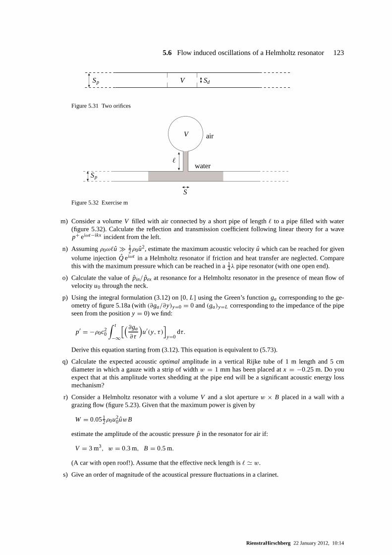
5.6 Flow induced oscillations of a Helmholtz resonator 123
Sp V Sd
Figure 5.31 Two orifices
S
V
`
air
waterSp
Figure 5.32 Exercise m
m) Consider a volumeV filled with air connected by a short pipe of length` to a pipe filled with water(figure 5.32). Calculate the reflection and transmission coefficient following linear theory for a wavep+ eiωt−ikx incident from the left.
n) Assumingρ0ω`u � 12ρ0u2, estimate the maximum acoustic velocityu which can be reached for given
volume injectionQ eiωt in a Helmholtz resonator if friction and heat transfer are neglected. Comparethis with the maximum pressure which can be reached in a1
4λ pipe resonator (with one open end).
o) Calculate the value ofpin/ pex at resonance for a Helmholtz resonator in the presence of mean flow ofvelocityu0 through the neck.
p) Using the integral formulation (3.12) on[0, L] using the Green’s functionga corresponding to the ge-ometry of figure 5.18a (with(∂ga/∂y)y=0 = 0 and(ga)y=L corresponding to the impedance of the pipeseen from the positiony = 0) we find:
p′ = −ρ0c20
∫ t
−∞
[(∂ga
∂τ
)u′(y, τ )
]y=0
dτ.
Derive this equation starting from (3.12). This equation isequivalent to (5.73).
q) Calculate the expected acousticoptimal amplitude in a vertical Rijke tube of 1 m length and 5 cmdiameter in which a gauze with a strip of widthw = 1 mm has been placed atx = −0.25 m. Do youexpect that at this amplitude vortex shedding at the pipe endwill be a significant acoustic energy lossmechanism?
r) Consider a Helmholtz resonator with a volumeV and a slot aperturew × B placed in a wall with agrazing flow (figure 5.23). Given that the maximum power is given by
W = 0.0512ρ0u2
0uwB
estimate the amplitude of the acoustic pressurep in the resonator for air if:
V = 3 m3, w = 0.3 m, B = 0.5 m.
(A car with open roof!). Assume that the effective neck length is` ' w.
s) Give an order of magnitude of the acoustical pressure fluctuations in a clarinet.
RienstraHirschberg 22 January 2012, 10:14
6 Spherical waves
6.1 Introduction
In the previous chapter we have considered the low frequencyapproximation of the acoustics ofpipes and resonators. Radiation of sound from such systems was assumed to be a small effect forthe internal acoustic field, and therefore could be neglected in our analysis. However, if sound wouldnot escape we would not hear it. Hence, for the calculation ofenvironmental noise the radiation iscrucial. Furthermore, as sound often is transferred through walls, the vibration of elastic structures isan essential part of the radiation path. To keep things manageable we will assume that the vibratingobjects are small compared to the wave length (compact bodies) and that we radiate sound into anunbounded homogeneous quiescent fluid (free space).
Starting from an exact solution of the acoustic field inducedby the pulsation and translation of a sphere(section 6.2) we will derive an expression for the free field Green’s functionG0 (6.36,6.37). Taylor’sseries expansion ofG0 will be used to introduce the concepts of monopole, dipole, quadrupole, etc,and multipole expansion (section 6.3). The method of imageswill appear to be a very powerful toolto get insight into the effect of boundaries on radiation (section 6.4). After a summary of the classicalapplication of Lighthill’s analogy to free jets (section 6.5) we will consider the radiation of a compactbody by using Curle’s formalism (section 6.6). This will be used to get insight into the sound generatedby a ventilator. Finally the radiation from an open pipe termination will be discussed (section 6.7).
Note. Two-dimensional acoustic waves have a complex structure asmay be seen from the Green’sfunctions given in Appendix E (see the discussion by Dowlinget al. [52]).
6.2 Pulsating and translating sphere
The wave equation in 3-D allows quite complex solutions. However, for the particular case of a spher-ically symmetric acoustic field the wave equation reduces to:
1
c20
∂2 p′
∂t2− 1
r 2
∂
∂r
(r 2∂p′
∂r
)= 0 (6.1)
wherer is the distance between the observation point and the origin. The key for solving (6.1) is thatwe can formulate a 1-D wave equation for (rp′):
1
c20
∂2(rp′)
∂t2− ∂2(rp′)
∂r 2= 0. (6.2)
This result can easily be understood because acoustic energy scales withp′2 (equation 2.80a). Hence,as the surface of a spherical wave increases withr 2 the amplitudep′(r ) should decrease asr −1 to keepenergy constant as the wave propagates.
6.2 Pulsating and translating sphere 125
Compared to 1-D waves the relationship between pressurep′ and acoustic velocityv′ now showsa drastically new behaviour which depends on the ratio ofr and the acoustic wave length. In threedimensions we have a region withkr � 1 called “near field” in which we find a behaviour ofv′ whichis close to that of an incompressible flow, while forkr � 1 we find a “far field” region in which thewaves behave locally as plane waves. The radius of curvatureof the wave front is large compared tothe wave length.
These features may be derived from the radial component of the (linearized) momentum conservationlaw:
ρ0∂v′
∂t= −∂p′
∂r(6.3a)
and the linearized mass conservation law:
∂(ρ ′r 2)
∂t= −ρ0
∂(v′r 2)
∂r. (6.3b)
The mass in a volume shell 4πr 2dr changes as a result of the difference between 4πr 2v′ and 4π(r +dr )2v′(r + dr ) in flux. We eliminateρ ′ by using the constitutive equationp′ = c2
0ρ′, and eliminatev′
by subtracting the time derivative ofr 2 times the momentum equation (6.3a) from the spatial derivativeof the mass equation (6.3b). This yields the wave equation (6.1).
The general, formal solution of (6.2) is:
rp′ = F(t − r
c0
)+ G
(t + r
c0
), (6.4)
combining an outgoing waveF and an incoming waveG. Far away there is no incoming wave, so wedefinethe “free field” as the region for whichG = 0. This result of a vanishing incoming wave in freespace may also be formulated as a boundary condition atr → ∞ (2.23a,2.23b,2.25).
As already stated, the acoustic velocityv′ has a rather complex behaviour, in contrast with the 1-Dsituation. This behaviour is found by substitution of (6.4)into the momentum conservation law (6.3a):
ρ0∂v′
∂t= 1
r 2F
(t − r
c0
)+ 1
c0rF ′
(t − r
c0
). (6.5)
We now observe that the first term of (6.5) corresponds, forr/c0 much smaller than the typical inherenttime scale, to an incompressible flow behaviour (r 2v′ = constant) while the second term correspondsto wave-like phenomena. Only the second term does contribute to the acoustic energy flux〈I 〉 =〈p′v′〉. This may be verified by substitution of a harmonic solution into (6.5):
p′ = p eiωt = A
4πreiωt−ikr (6.6)
we find
v = p
iωρ0r+ p
ρ0c0= p
ρ0c0
(− i
kr+ 1
). (6.7)
The first term inv is 12π out of phase withp and therefore does not contribute to〈I 〉 = 〈p′v′〉. Hence:
〈p′v′〉 = 14(v p∗ + v∗ p) = p p∗
2ρ0c0. (6.8)
RienstraHirschberg 22 January 2012, 10:14
126 6 Spherical waves
A very systematic discussion of this fundamental solution is given by Lighthill [121].
Using (6.5) we can now determine the acoustic field generatedby a pulsating sphere of radiusa(t). If(∂a/∂t)/c0 � 1, we can use linear acoustics, while the movement of the sphere boundary yields theequation derived from (6.5):
ρ0∂2a
∂t2= 1
a2F
(t − a
c0
)+ 1
c0aF ′
(t − a
c0
). (6.9)
For a compact sphere the first term is dominating(a(∂2a/∂t2)/c20 � 1). We find exactly the result
which we could anticipate from (2.61), the second derivative to time of the volume of the sphere isthe source of sound.
A steady expansion of the sphere (∂a/∂t = constant) does not (in this approximation) generate sound.The second term of (6.9) is dominating for large sphere radii(a(∂2a/∂t2)/c2
0 � 1). In such a case theaction of the wall movement is that of a piston which generates plane waves. For harmonic oscillationsof the sphere(a = a0+a eiωt), the amplitudeA of the radiated field is found from (6.6) by substitutionof v = iωa in (6.7) atr = a0.
p(a0) = A
4πa0e−ika0 = − ω2ρ0a
1 + i ka0.
Hence
p(r ) = − ω2ρ0aa0
(1 + i ka0)2e−ik(r−a0) . (6.10)
We can also determine the acoustic impedanceZ
Z(ω) = p(a0)
v(a0)= p(a0)
iωa(6.11)
Using (6.7) we find:
Z
ρ0c0= i ka0
1 + i ka0= i ka0 + (ka0)
2
1 + (ka0)2. (6.12)
We see that the real part of the radiation impedance of a compact sphere (ka0 � 1) is very small:
Re( Z
ρ0c0
)' (ka0)
2 (6.13)
Hence (see (3.17)) a compact vibrating object in free space will be a very ineffective source of sound.This effect becomes even more dramatic when we consider the radiation of a compact vibrating ob-ject of constant volume. The most simple example of this behaviour is a translating sphere of constantradiusa0. This is what we call a dipole radiation source, in contrast to the monopole source corre-sponding to a compact pulsating sphere.
The solution of the problem is easily obtained since we can generate from the spherically symmetricsolution (6.4) non-spherically symmetric solutions by taking a spatial derivative (see equation 2.24b).If ϕ′ is a (spherically symmetric) solution of the wave equation:
1
c20
∂2ϕ′
∂t2− ∇2ϕ′ = 0 (6.14)
RienstraHirschberg 22 January 2012, 10:14
6.2 Pulsating and translating sphere 127
then any derivative ofϕ′, such as(∂ϕ′/∂xi ) or (∂ϕ′/∂t), is also a solution:
1
c20
∂2
∂t2
(∂ϕ′
∂xi
)− ∇2
(∂ϕ′
∂xi
)= 0, (6.15)
in particular, any derivative of Eq. (6.6) is a solution. So if we try to find the field of a translatingsphere with velocityv0 (in x-direction), where at its surface the radial flow velocity isgiven by:
v′(a0, ϑ) = v0· ra0
∣∣∣|r |=a0
= v0 cosϑ. (6.16)
we can use the derivative in thex-direction. For a harmonic oscillationv0 = v0 eiωt with (v0/ωa0) � 1the pressure fieldp′ is given by:
p = A∂
∂x
(e−ikr
r
)= Acosϑ
∂
∂r
(e−ikr
r
)(6.17)
because∂ r∂x = cosϑ . This pressure is related to the acoustic velocityv′ by the momentum conservation
law (6.3a):
iωρ0v = −Acosϑ∂2
∂r 2
(e−ikr
r
). (6.18)
Using the boundary condition (6.16) forr = a0 we can now calculate the amplitudeA for given v0:
iωv0 = −A2 + 2ika0 − (ka0)
2
a30
e−ika0 (6.19)
so that the pressure field (6.17) can be written as:
p = −iωρ0v0a30 cosϑ
2 + 2ika0 − (ka0)2
∂
∂r
(e−ik(r−a0)
r
). (6.20)
In the limit of (ka0) � 1 we see that:
p ' −12(ka0)
2ρ0c0v0a0 cosϑ
r
(1 − i
kr
)e−ikr . (6.21)
Again we observe a near field behaviour with a pressure decreasing asr −2 and for which p is 12π
out of phase withv0. This pressure field simply corresponds to the inertia of theincompressible flowinduced by the movement of the fluid from the front towards theback of the moving sphere. From(6.21) forr = a0 with (ka0) � 1 we see that:
p(a0) ' 14ρ0c0v0 cosϑ
(2ika0 + i (ka0)
3 + (ka0)4) . (6.22)
Hence, as the drag on the sphere, which is in phase withv0, scales asa20 Re[ p(a0)], we see that the
acoustic power generated by the sphere scales asρ0c0v20a2
0(ka0)4. This is a factor(ka0)
2 weaker thanthe already weak radiation power of a compact pulsating sphere. So we now understand the need ofa body in string instruments or of a sound board in a piano. While the string is a compact oscillatingcylinder (row of oscillating spheres), which does not produce any significant sound directly, it inducesvibrations of a plate which has dimensions comparable with the acoustic wave length and hence is
RienstraHirschberg 22 January 2012, 10:14
128 6 Spherical waves
radiating with an acoustic impedanceρ0c0 which is a factor(ka0)4 more efficient than direct radiation
by the string.
Note. In order to provide a stable sound one should avoid in string instruments elastic resonances ofthe body which are close to that of the string. If this is not the case the two oscillators start a complexinteraction, which is called for a violin a “wolf tone”, because it has a chaotic behaviour [129].
Having discussed aspects of bubble acoustics in a pipe in section 4.4.5, we will now consider somespecific free field effects. Consider the oscillation of a compact air bubble in water as a response toan incident plane wavepin = pin eiωt−ikx in free space (deep under water). We can locally assumethe pressurepb in the bubble to be uniform and we assume a spherical oscillation of the bubble ofequilibrium radiusa0:
a = a0 + a eiωt . (6.23)
The pressure in the bubble is given by:
p′b = p′
in + p′r (a0) (6.24)
wherep′r (a0) is the acoustic pressure due to the spherical waves generated by the bubble oscillation.
We have neglected surface tension. Furthermore, we assume an ideal gas behaviour in the bubble:
p′b
p0= −3γ
a′
a0(6.25)
whereγ = 1 for isothermal compression andγ = CP/CV for isentropic compression.pr (a) is relatedto a by the impedance condition:
pr (a) = iωaZ (6.26)
andZ(ω) is given by equation (6.12). Hence combining (6.24) with (6.25) and (6.26) we find:
− 3γ p0
a0a = pin + iωaZ (6.27)
or:
pr (a0) = iωaZ = − pin
1 − i3γ p0
ωa0Z
(6.28)
and
pr = pr (a0)a0
re−ik(r−a0) . (6.29)
Using (6.12) we can write (6.28) as:
pr (a0) = − pin
1 −(ω0
ω
)2(1 + i ka0
) (6.30)
whereω0 is the Minnaert frequency defined by:
ω20 = 3γ p0
ρ0a20
. (6.31)
RienstraHirschberg 22 January 2012, 10:14

6.3 Multipole expansion and far field approximation 129
It is interesting to note that at resonance (ω = ω0) under typical conditions a bubble is compactbecause:
(k0a0)2 =
(ω0a0
c0
)2= 3γ p0
ρ0c20
(6.32)
is small as long asp0 � ρ0c20.
For waterρ0c20 = 2 × 10⁴ bar, hence up top0 = 100 bar one can still assume bubble oscillations
at resonance to be compact. Equation (6.30) has many interesting further applications [52, 113]. Forexample, sonar detection of fishes by using a sweeping incident sound frequency yields informationabout the size of fishes because the resonance frequencyω0 of the swim bladder yields informationon the sizea0 of the fish. Furthermore, at resonance sound is scattered quite efficiently:
pr = −ipin
k0re−ik(r−a0) . (6.33)
Hence the fish scatters sound with an effective cross sectionof the order of the acoustic wave lengthat ω0 (an effective increase of the cross section by a factor(k0a0)
−1). As we knowa0 from ω0 theintensity of the scattered field yields information on the amount of fish. Another fascinating effect ofbubble resonance is the very specific sound of rain impact on water [178].
6.3 Multipole expansion and far field approximation
The free field Green’s functionG0 defined by equation (3.1)
∂2G0
∂t2− c2
0
∑ ∂2G0
∂x2i
= δ(x − y)δ(t − τ) (3.1)
and the Sommerfeld radiation condition (2.25), may be foundin Appendix E, but can be derived asfollows. We start with considering the Fourier transformG0 of G0, with
G0 =∫ ∞
−∞G0 eiωt dω
and satisfying
∑ ∂2G0
∂x2i
+ k2G0 = − 1
2πc20
δ(x − y)e−iωτ , (6.34)
wherek = ω/c0. From symmetry arguments,G0 can only be a function of distancer = |x − y|, sothe solution of (6.34) has the form (see equation (6.6))
G0 = A
4πre−ikr (6.35)
where A is to be determined. Integration of (6.34) over a small sphere Bε around y, given by, say,r = ε, yields by application of Gauss’ theorem
∫∫∫
Bε
∑ ∂2G0
∂x2i
+ k2G0 dx =∫∫∫
Bε
− 1
2πc20
δ(x − y)e−iωτ dx =
∫∫
∂Bε
∑ ∂G0
∂xini dσ +
∫∫∫
Bε
k2G0 dx = 4πε2∂G0
∂r+ O(ε2) = −A + O(ε) = − 1
2πc20
e−iωτ
RienstraHirschberg 22 January 2012, 10:14

130 6 Spherical waves
whereni denotes the outward normal ofBε, and we used the fact thatε is small. If we letε → 0 wefind thatA = (2πc2
0)−1 e−iωτ . So we have:
G0 = e−iωτ−ikr
8π2c20r
= e−iω(τ+r/c0)
8π2c20r
(6.36)
(note the factor−1/2π difference with the Green’s function of a regular Helmholtzequation) and,using equation (C.33),
G0 = δ(t − τ − r/c0)
4πrc20
. (6.37)
In order to derive the general multipole expansion we will first consider the field at a single frequency.By using the free-field Green’s function (Appendix E) we find the acoustic field for a given time-harmonic source distributionq(x)eiωt in a finite volumeV to be given by
ρ ′ = p′
c20
=∫∫∫
V
q(y)G0(x|y)dy =∫∫∫
V
q(y)e−ikr
4πc20r
dy. (6.38)
Suppose the origin is chosen insideV . We are interested in the far field,i.e. |x| is large, and a compactsource,i.e. kL is small whereL is the typical diameter ofV. This double limit can be taken inseveral ways. As we are interested in the radiation properties of the source, which corresponds withk|x| > O(1), we will keepkx fixed. In that case the limit of smallk is the same as smally, and wecan expand in a Taylor series aroundy = 0
r =(|x|2 − 2(x · y)+ |y|2
)1/2 = |x|(1 − x· y
|x|2 + |y|22|x|2 − (x· y)2
2|x|4 + . . .)
= |x|(1 − |y|
|x| cosθ + 12
|y|2|x|2 sin2 θ + . . .
)
(whereθ is the angle betweenx and y) and
e−ikr
r= e−ik|x|
|x|(1 +
(1 + i k|x|
) 1
|x|23∑
j =1
x j y j + . . .)
=∞∑
l ,m,n=0
yl1ym
2 yn3
l ! m! n!
[∂ l+m+n
∂yl1∂ym
2 ∂yn3
e−ikr
r
]
y1=y2=y3=0
. (6.39)
As r is a symmetric function inx and y, this is equivalent to
e−ikr
r=
∞∑
l ,m,n=0
(−1)l+m+n
l ! m! n! yl1ym
2 yn3
∂ l+m+n
∂xl1∂xm
2 ∂xn3
e−ik|x|
|x| . (6.40)
The acoustic field is then given by
ρ ′ = 1
4πc20
∞∑
l ,m,n=0
(−1)l+m+n
l ! m! n!
∫∫∫
V
yl1ym
2 yn3 q(y)dy
∂ l+m+n
∂xl1∂xm
2 ∂xn3
e−ik|x|
|x| . (6.41)
As each term in the expansion is by itself a solution of the reduced wave equation, this series yieldsa representation in which the source is replaced by a sum of elementary sources (monopole, dipoles,
RienstraHirschberg 22 January 2012, 10:14
6.3 Multipole expansion and far field approximation 131
quadrupoles, in other words, multipoles) placed at the origin (y = 0). Expression (6.41) is the mul-tipole expansion of a field from a finite source in Fourier domain. From this result we can obtain thecorresponding expansion in time domain as follows.
With Green’s function (6.37) we have the acoustic field from asourceq(x, t)
ρ ′ =∫ ∞
−∞
∫∫∫
V
q(y, τ )δ(t − τ − r/c0)
4πrc20
dydτ =∫∫∫
V
q(y, t − r/c0)
4πrc20
dy (6.42)
If the dominating frequencies in the spectrum ofq(x, t) are low, such thatωL/c0 is small, we obtainby Fourier synthesis of (6.41) the multipole expansion in time domain (see Goldstein [70])
ρ ′ = 1
4πc20
∞∑
l ,m,n=0
(−1)l+m+n
l ! m! n!∂ l+m+n
∂xl1∂xm
2 ∂xn3
1
|x|
∫∫∫
V
yl1ym
2 yn3 q(y, t − |x|/c0)dy
=∞∑
l ,m,n=0
∂ l+m+n
∂xl1∂xm
2 ∂xn3
[(−1)l+m+n
4π |x|c20
µlmn(t − |x|/c0)
](6.43)
whereµlmn(t) is defined by:
µlmn(t) =∫∫∫
V
yl1ym
2 yn3
l ! m! n! q(y, t)dy. (6.44)
The (lmn)-th term of the expansion (6.43) is called a multipole of order 2l+m+n. Since each termis a function of|x| only, the partial derivatives toxi can be rewritten into expressions containingderivatives to|x|. In general, these expressions are rather complicated, so we will not try to givethe general formulas here. It is, however, instructive to consider the lowest orders in more detail asfollows.
The first term corresponds to the monopole:
ρ ′0 = µ0(t − |x|/c0)
4πc20|x|
(6.45)
where we wrote for brevityµ0 = µ000. We have concentrated the source at the origin and
µ0(t) =∫∫∫
V
q(y, t)dy. (6.46)
The next term is the dipole term:
ρ ′1 = −
3∑
i=1
xi
|x|∂
∂|x|(µ1,i (t − |x|/c0)
4πc20|x|
)(6.47)
where we wrote for brevity:µ1,1 = µ100, µ1,2 = µ010 andµ1,3 = µ001. If q is a point source thisdipole term is easily visualized as shown in figure 6.1.
The dipole of strengthµ1,i , which we should place at the origin (y = 0):
µ1,i (t) =∫∫∫
V
yi q(y, t)dy, (6.48)
RienstraHirschberg 22 January 2012, 10:14

132 6 Spherical waves
.....
Figure 6.1 First step in the multipole expansion of a point source.
is obtained by bringing the (point) sourceq towards the origin while increasing its strength and thatof the opposite (point) source−q at the origin in such a way that we keep|y|q constant.
A dipole field is not isotropic because in a direction normal to the vectory the two sources formingthe dipole just compensate each other, while in the other directions due to a difference in emissiontime there is a net acoustic field. This effect of the difference in retarded time (figure 6.2) between the
ϑ
y
x
x − y
y·x|x|
Figure 6.2 Retarded or emission time difference is( y·x/|x|)/c0 = (|y| cosϑ)/c0.
sources in the dipole simplifies in the far field as follows. Writing (6.47) as:
ρ ′1 = −
3∑
i=1
xi
|x|
∫∫∫
V
yi
4πc20
{− 1
c0|x|∂
∂tq(y, t − |x|/c0)− 1
|x|2 q(y, t − |x|/c0)
}dy (6.49)
we see that for large distances (k|x| � 1) the acoustic field due to the dipole contribution is given by:
ρ ′1 '
3∑
i=1
xi
4πc30|x|2
∂
∂t
∫∫∫
V
yi q(y, t − |x|/c0)dy =3∑
i=1
xi
4πc30|x|2
[ d
dteµ1,i (te)
]te=t−|x|/c0
(6.50)
whereµ1,i (t) is the dipole strength. If the source has a particular form, for example it represents aforce densityfi like in (2.65):
q(y, τ ) = −3∑
i=1
∂ f i
∂yi, (6.51)
we observe that the surface integral of the monopole term vanishes because we assumed a finitesource region, outside whichf = 0. We see that the force fieldfi is equivalent to an acoustic dipole
RienstraHirschberg 22 January 2012, 10:14
6.4 Method of images and influence of walls on radiation 133
of strength:
µ1,i =∫∫∫
V
fi dy (6.52)
which corresponds simply to the total forceF on V . In a similar way it is clear that the Lighthill stresstensorTi j induces a quadrupole field because from (2.65) we have:
q =3∑
i, j =1
∂2Ti j
∂yi∂y j.
By partial integration it follows that the strength of the quadrupole is:
µ2,i j =∫∫∫
V
Ti j dx, (6.53)
where we wrote for brevityµ2,11 = µ200, µ2,12 = µ110, µ2,13 = µ101, etc. . In the far field ap-proximation, where the retarded (or emission) time effect can be estimated by replacing(∂/∂|x|) by−c−1
0 (∂/∂t), we find for a quadrupole field
ρ ′ '3∑
i, j =1
xi x j
4πc20|x|3
1
c20
[ d2
dt2e
µ2,i j (te)]
te=t−|x|/c0
. (6.54)
6.4 Method of images and influence of walls on radiation
Using G0 we can build the Green’s function in presence of walls by using the method of images asdiscussed in section 4.6. The method of images is simple for aplane rigid wall and for a free surface.In the first case the boundary conditionv′ ·n = 0 is obtained by placing an image of equal strengthq at the image point of the source position (figure 6.3). For a free surface, defined by the conditionp′ = 0 (air/water interface seen from the water side), we place anopposite source−q at the imagepoint.
For a rigid wall atx1 = 0 we simply have the Green’s function:
G(x, t|y, τ ) = δ(t − τ − r/c0)
4πc20r
+ δ(t − τ − r ∗/c0)
4πc20r ∗ (6.55)
where
r =√(x1 − y1)2 + (x2 − y2)2 + (x3 − y3)2,
r ∗ =√(x1 + y1)2 + (x2 − y2)2 + (x3 − y3)2.
We easily see from figure 6.3 that a source placed close to a rigid wall will radiate as a source ofdouble strength (|y1|k � 1) while a source close to a free surface will radiate as a dipole.
When more than a wall is present the method of images can be used by successive reflections againstthe walls. This is illustrated in figure 6.4. When a harmonic source is placed half way between tworigid walls separated by a distanceh (at y = 1
2h) the radiated field is equivalent to that of an infinite
RienstraHirschberg 22 January 2012, 10:14
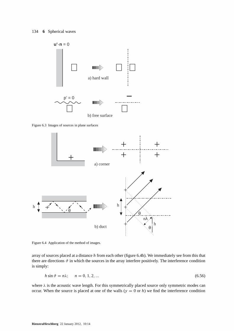
134 6 Spherical waves
+ ++
+ +−
b) free surface
a) hard wall
p’ = 0
u’.n = 0
Figure 6.3 Images of sources in plane surfaces
nλ
h
h
θ
θb) duct
a) corner
hθ
Figure 6.4 Application of the method of images.
array of sources placed at a distanceh from each other (figure 6.4b). We immediately see from this thatthere are directionsϑ in which the sources in the array interfere positively. The interference conditionis simply:
h sinϑ = nλ; n = 0,1,2, ... (6.56)
whereλ is the acoustic wave length. For this symmetrically placed source only symmetric modes canoccur. When the source is placed at one of the walls (y = 0 or h) we find the interference condition
RienstraHirschberg 22 January 2012, 10:14
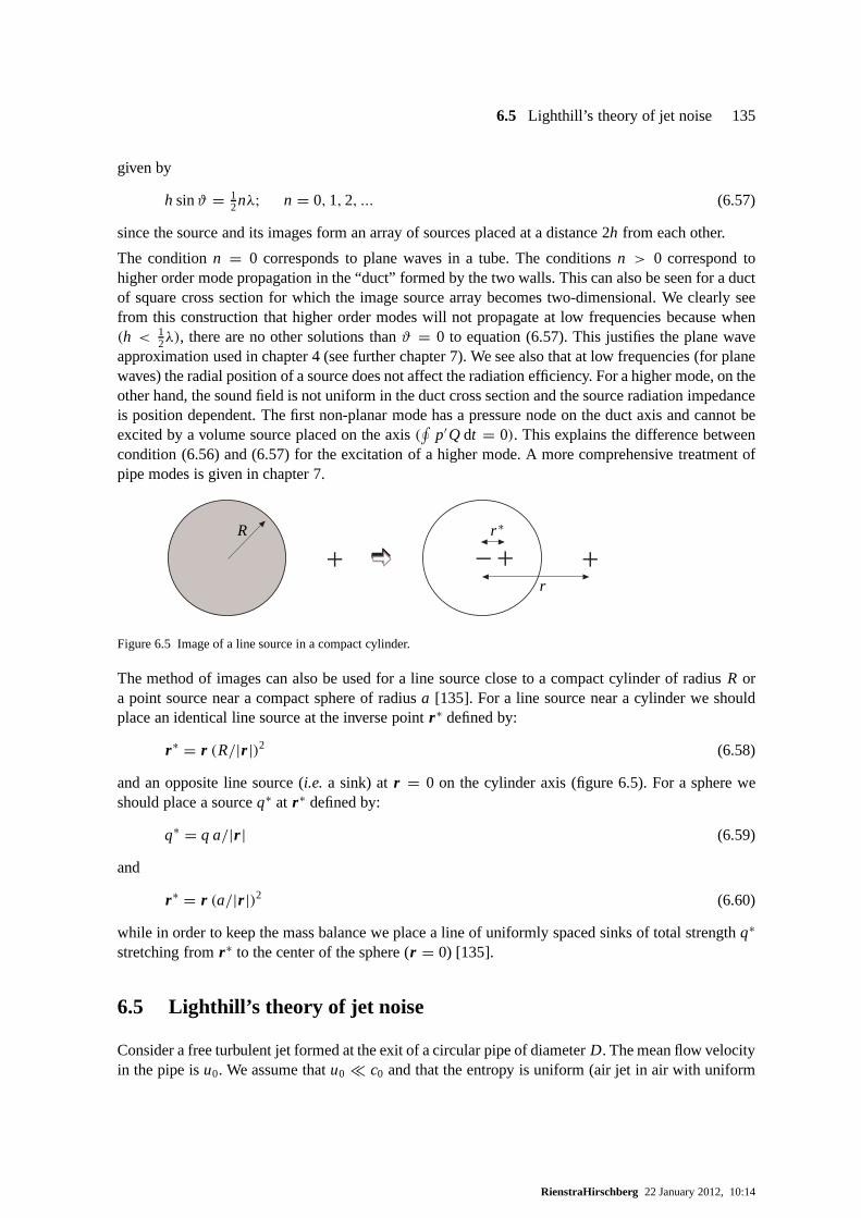
6.5 Lighthill’s theory of jet noise 135
given by
h sinϑ = 12nλ; n = 0,1,2, ... (6.57)
since the source and its images form an array of sources placed at a distance 2h from each other.
The conditionn = 0 corresponds to plane waves in a tube. The conditionsn > 0 correspond tohigher order mode propagation in the “duct” formed by the twowalls. This can also be seen for a ductof square cross section for which the image source array becomes two-dimensional. We clearly seefrom this construction that higher order modes will not propagate at low frequencies because when(h < 1
2λ), there are no other solutions thanϑ = 0 to equation (6.57). This justifies the plane waveapproximation used in chapter 4 (see further chapter 7). We see also that at low frequencies (for planewaves) the radial position of a source does not affect the radiation efficiency. For a higher mode, on theother hand, the sound field is not uniform in the duct cross section and the source radiation impedanceis position dependent. The first non-planar mode has a pressure node on the duct axis and cannot beexcited by a volume source placed on the axis(
∮p′Q dt = 0). This explains the difference between
condition (6.56) and (6.57) for the excitation of a higher mode. A more comprehensive treatment ofpipe modes is given in chapter 7.
R r∗
r
Figure 6.5 Image of a line source in a compact cylinder.
The method of images can also be used for a line source close toa compact cylinder of radiusR ora point source near a compact sphere of radiusa [135]. For a line source near a cylinder we shouldplace an identical line source at the inverse pointr∗ defined by:
r∗ = r (R/|r|)2 (6.58)
and an opposite line source (i.e. a sink) atr = 0 on the cylinder axis (figure 6.5). For a sphere weshould place a sourceq∗ at r∗ defined by:
q∗ = q a/|r| (6.59)
and
r∗ = r (a/|r|)2 (6.60)
while in order to keep the mass balance we place a line of uniformly spaced sinks of total strengthq∗
stretching fromr∗ to the center of the sphere (r = 0) [135].
6.5 Lighthill’s theory of jet noise
Consider a free turbulent jet formed at the exit of a circularpipe of diameterD. The mean flow velocityin the pipe isu0. We assume thatu0 � c0 and that the entropy is uniform (air jet in air with uniform
RienstraHirschberg 22 January 2012, 10:14
136 6 Spherical waves
temperature). The key idea of Lighthill was that the sound produced by the turbulence was originatedfrom a volume of orderD3 and that the influence of the pipe walls on the sound radiationcould beneglected.
In such a case combining (2.65) with (3.13) and using the freespace Green’s functionG0 given by(6.37) we find:
ρ ′(x, t) =t∫
−∞
∫∫∫
V
∂2Ti j
∂yi∂y jG0(x, t|y, τ )dydτ. (6.61)
Partial integration (twice) yields:
ρ ′(x, t) =t∫
−∞
∫∫∫
V
∂2G0
∂yi∂y jTi j (y, τ )dydτ. (6.62)
BecauseG0 is only a function ofr = |x − y| we have:
∂G0
∂yi= ∂G0
∂r
∂r
∂yi= −
(xi − yi
r
)∂G0
∂r= −∂G0
∂xi. (6.63)
Approaching the source towards the observation point has the same effect as approaching the obser-vation point towards the source. Hence we can write (6.62) as:
ρ ′(x, t) = ∂2
∂xi ∂x j
t∫
−∞
∫∫∫
V
G0(x, t|y, τ )Ti j (y, τ )dydτ. (6.64)
The integration variableyi does not interfere withxi . Using now (6.37) we can carry out the timeintegration:
ρ ′(x, t) = ∂2
∂xi ∂x j
∫∫∫
V
Ti j (y, t − r/c0)
4πc20r
dy. (6.65)
In the far field the only length scale is the wave length, hencewe have replaced the problem of theestimate of a space derivative(∂/∂yi ) at the source by the problem of the estimate of the characteristicfrequency of the produced sound. In the far field approximation we have:
ρ ′(x, t) ' xi x j
4πc20|x|2
∂2
c20∂t2
∫∫∫
V
Ti j (y, t − |x|/c0)
|x| dy. (6.66)
For high Reynolds number we can neglect the effect of viscosity (if it were not small turbulence wouldnot occur!). If we assume a homentropic compact flow we have (2.68):
Ti j ' ρ0viv j . (6.67)
The first estimates of Lighthill for a circular1 free jet are:
1See Bjørnø [15] for planar jets.
RienstraHirschberg 22 January 2012, 10:14

6.5 Lighthill’s theory of jet noise 137
– the characteristic time scale for large eddy’s in the flow is (D/u0).– the Reynolds stress scales asρu2
0.– the relevant volumeV is of orderD3.
Hence we should replace(∂/∂t) by u0/D in (6.66) and we find:
ρ ′(x, t) ∼ 1
4πc40
(u0
D
)2ρ0u20D3
|x| (6.68)
or in terms of intensityρ ′2 and Mach numberM0 = u0/c0:
ρ ′2 ∼( ρ0D
4π |x|)2
M80 . (6.69)
This is the celebrated 8-th power law of Lighthill which ".. represents a triumph of theory over ex-periment; before the publication ofU8, most reports of measured jet noise data gave aU4 variation,which was then quickly recognized, postU8, as associated with noise sourceswithin the engine itself,rather than with the jet exhaust turbulent mixing downstream of the engine. In fact, variation of in-tensity withU8 is now generally accepted asdefiningjet mixing noise .." (Crighton, l.c.); see figure6.6. Equation (6.69) tells us that turbulence in free space is a very ineffective source of sound. Whena more detailed description of the flow is used to estimateTi j one can also find the directivity patternof the radiation field [70, 16, 185]. This directivity pattern results from Doppler effects and refractionof the sound waves by the shear layer surrounding the jet.
300 650 1400 300014065
200
180
160
140
120
100
80
model curves
SP
L (d
B)
jet enginesrockets
U8
U3
U [m/s]
Figure 6.6 Sound power generated by a jet.
As the Mach number approaches unity the character of the sound production changes drasticallybecause the flow is not compact any more (D/λ ∼ M0) and because at higher Mach numbers shockwaves appear if the jet is not properly expanded. These shocks generate noise by interaction withturbulence (random vorticity) and vortices (coherent structures) [66].
Moreover, it is obvious that the generated power cannot growindefinitely with a powerM8. Thereis a natural maximum corresponding to the kinetic energy fluxin the jet 1
2ρu30 · π4 D2. This natural
upper bound prevails aboveM > 1 and the sound intensity scales aboveM > 1 asM30 . The typical
fraction of flow power transferred to the acoustic field at high Mach number by a properly expanded
RienstraHirschberg 22 January 2012, 10:14
138 6 Spherical waves
supersonic jet is 10−4 (M > 1). Following Goldstein [70] the acoustic powerW generated by asubsonic homentropic jet is given by
W18ρ0u3
0πD2= 8 × 10⁻⁵M5
0 . (6.70)
Hence at MachM0 = 0.1 we can estimate that only a fraction 10−9 of the hydrodynamic power istransferred to the acoustic field. This is the key of the problem of calculating the acoustic field froma numerical calculation of the flow pattern at low Mach numbers. In order to achieve this we haveto calculate the flow field within an accuracy which is far above the typical score (5%) of turbulencemodelling nowadays. However, the simple scaling law of Lighthill already tells us that in order toreduce turbulence noise we should reduce the Mach number. A very useful result as we will see fromexercise k) below.
Lighthill’s analogy in the form of equation (6.66) is often used to obtain acoustical information fromnumerical calculations of turbulent flow. Such calculations can be based on an incompressible modelwhich by itself does not include any acoustic component.
When the jet has a different entropy than the environment (hot jet or different fluid) the sound pro-duction at low Mach numbers is dominated by either Morfey’s dipole source term(∂/∂yi )((c2 −c2
0)/c20)(∂p′/∂yi ) or by a volume source term due to diffusion and heat transfer (entropy fluctuations).
When a hot gas with constant caloric properties is mixed withthe cold environment the monopolesound source is negligible compared to the dipole due to convective effects ([139]). One finds then asound power which at low Mach numbers scales atM6
0 . Upon increasing the Mach number the tur-bulent Reynolds stress can become dominant and a transitionto the cold jet behaviour(M8
0) can beobserved in some cases.
In hot jets with combustion, vapour condensation or strongly temperature dependent caloric gas prop-erties the monopole source dominates ([42]), and a typicalM4
0 scaling law is found forρ ′2.
The influence of the viscosity on the sound generation by a free jet has been studied by Morfey [140],Obermeier [160] and Iafrati [90].
6.6 Sound radiation by compact bodies in free space
6.6.1 Introduction
In principle, when a compact body is present in a flow we have two possible methods to calculatethe sound radiation when using Lighthill’s theory (section2.6). In the first case we use atailoredGreen’s function which is often easy to calculate in the far field approximation by using the reciprocityprinciple (3.4). In the second case we can use thefree fieldGreen’s functionG0 which implies thatwe should take surface contributions in equation (3.12) into account. This second method is calledCurle’s method [70, 16]. The advantage of the method of Curleis that we still can use the symmetryproperties ofG0 like:
∂G0
∂yi= −∂G0
∂xi. (6.71)
Furthermore, we will see that the surface terms have for compact rigid bodies quite simple physicalmeaning. We will see that the pulsation of the volume of the body is a volume source while the force
RienstraHirschberg 22 January 2012, 10:14

6.6 Sound radiation by compact bodies in free space 139
on the body is an aero-acoustic dipole. In this way we can in fact say that if we know the aerodynamic(lift and drag) force on a small propeller we can represent the system by the reaction force acting onthe fluid as an aero-acoustic source, ignoring further the presence of the body in the calculation of theradiation.
6.6.2 Tailored Green’s function
The method of tailored Green’s function has of course the nice feature of a simple integral equation(3.13). We will, however, in general not have a simple symmetry relation allowing to move the spacederivative outside the integral. The construction of the tailored Green’s function in the far field ap-proximation is in fact equivalent to considering the acoustic response of the body to a plane incidentwave. In applications like the effect of a bubble on turbulence noise we already did this for a bubblein a duct (section 4.7).
The method of images discussed in section 6.4 is an efficient procedure to construct a Green’s functionfor simple geometries. This is obvious when we consider a plane rigid wall. Using the reciprocityprinciple we send a plane wavep′
in and look at the resulting acoustic field in the source pointy. Theacoustic field iny is built out of the incident wavep′
in and the wave reflected at the surfacep′r . In the
method of images we simply assume thatp′r comes from an image source, as shown in figure 6.7.
a) b)
x x
y y
p′in
p′r
source
image
Figure 6.7 a) Acoustic response to a plane wave. b) Sound emitted by the source in the same observers direction.
When calculating the Green’s function we should take in freespace as amplitude of the incident wavep′
in the amplitude calculated from (6.37). For compact bodies orsources close to a surface we canneglect the variation in travel time ofp′
in over the source region and we find:
p′in = δ(−t + τ − |x|/c0)
4π |x|c20
(6.72)
where the signs oft andτ have been changed because of reciprocity relation (3.4). When consideringharmonic waves we have from (6.36) that:
pin = e−ikr
8π2c20r
(6.73)
where in the far field approximationr ' |x|. The Green’s function is found by adding the systemresponsep′
r (or pr ) to the incident wavep′in. Once a tailored Green’s function has been obtained we
RienstraHirschberg 22 January 2012, 10:14

140 6 Spherical waves
find by using (3.13):
ρ ′(x, t) =t∫
−∞
∫∫∫
V
q(y, τ )G(x, t|y, τ )dydτ. (3.13)
By partial integration and assuming that the sources are thevolume sources∂2Ti j /∂xi ∂x j as definedin (2.65) which are limited to a small region of space we find:
ρ ′(x, t) =t∫
−∞
∫∫∫
V
∂2G
∂yi∂y jTi j dydτ. (6.74)
Comparison of the space derivative of the tailored Green’s function with that of the free space Green’sfunctionG0 yields an amplification factorA of the radiated field:
A =∣∣∣ ∂
2G
∂yi∂y j
∣∣∣/∣∣∣ 1
c20
∂2G0
∂t2
∣∣∣ (6.75)
where we made use of the approximation∂2G0/∂xi ∂x j ' (∂2G0/∂t2)/c20 in the far field, and assumed
that the flow is not influenced by the foreign body (Ti j = constant).
Using this procedure one can show [16, 52, 70] that turbulence near the edge of a semi-infinite planeproduces a sound field for whichρ ′2 scales asM5
0 which implies forM0 � 1 a dramatic increase(by a factorM−3
0 ) compared to free field conditions. This contribution to trailing edge noise is veryimportant in aircraft noise and wind turbine noise.
6.6.3 Curle’s method
When we place a cylinder of diameterd in a turbulent jet with a main flow velocityu0, the cylinderwill not only enhance the radiation by the already present turbulence. A cylinder will affect the flow.Behind the cylinder at high Reynolds numbers we have an unstable wake. Above a Reynolds numberof Re = u0d/ν = 40 the wake structure is dominated by periodic vortex shedding if 40 6 Re 6
3 × 10⁵ and forRe > 3.5 × 10⁶ [16, 18, 75]. The frequencyfV of the vortex shedding is roughlygiven by:
fVd
u0= 0.2. (6.76)
Hence the sound produced by vortex shedding has in contrast with turbulence a well-defined fre-quency. The periodic shedding of vorticity causes an oscillating lift force on the cylinder, with anamplitudeL per unit length given by
L = −ρ00u0, (6.77)
where0 is the circulation of the flow around the cylinder. By definition the lift force is perpendicularto the mean flow direction(u0). In dimensionless form the lift is expressed as a lift coefficient CL :
CL = L12ρu2
0d. (6.78)
RienstraHirschberg 22 January 2012, 10:14
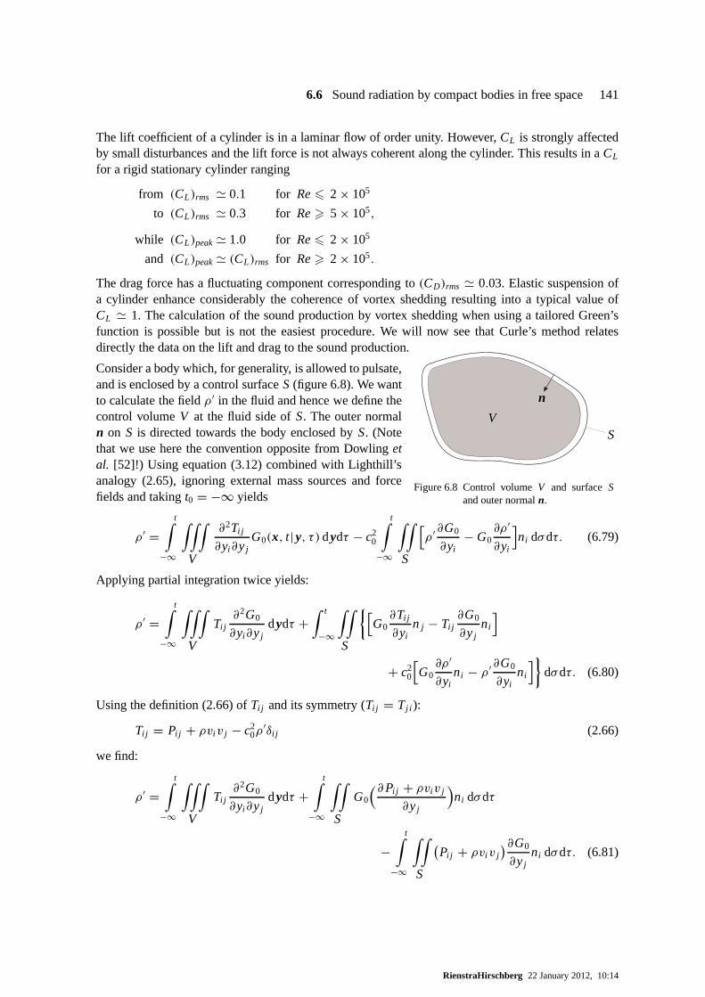
6.6 Sound radiation by compact bodies in free space 141
The lift coefficient of a cylinder is in a laminar flow of order unity. However,CL is strongly affectedby small disturbances and the lift force is not always coherent along the cylinder. This results in aCL
for a rigid stationary cylinder ranging
from (CL)rms ' 0.1 for Re6 2 × 10⁵
to (CL)rms ' 0.3 for Re> 5 × 10⁵,
while (CL)peak' 1.0 for Re6 2 × 10⁵
and (CL)peak' (CL)rms for Re> 2 × 10⁵.
The drag force has a fluctuating component corresponding to(CD)rms ' 0.03. Elastic suspension ofa cylinder enhance considerably the coherence of vortex shedding resulting into a typical value ofCL ' 1. The calculation of the sound production by vortex shedding when using a tailored Green’sfunction is possible but is not the easiest procedure. We will now see that Curle’s method relatesdirectly the data on the lift and drag to the sound production.
S
n
V
Figure 6.8 Control volumeV and surfaceSand outer normaln.
Consider a body which, for generality, is allowed to pulsate,and is enclosed by a control surfaceS (figure 6.8). We wantto calculate the fieldρ ′ in the fluid and hence we define thecontrol volumeV at the fluid side ofS. The outer normaln on S is directed towards the body enclosed byS. (Notethat we use here the convention opposite from Dowlingetal. [52]!) Using equation (3.12) combined with Lighthill’sanalogy (2.65), ignoring external mass sources and forcefields and takingt0 = −∞ yields
ρ ′ =t∫
−∞
∫∫∫
V
∂2Ti j
∂yi∂y jG0(x, t|y, τ )dydτ − c2
0
t∫
−∞
∫∫
S
[ρ ′ ∂G0
∂yi− G0
∂ρ ′
∂yi
]ni dσdτ. (6.79)
Applying partial integration twice yields:
ρ ′ =t∫
−∞
∫∫∫
V
Ti j∂2G0
∂yi∂y jdydτ +
∫ t
−∞
∫∫
S
{[G0∂Ti j
∂yin j − Ti j
∂G0
∂y jni
]
+ c20
[G0∂ρ ′
∂yini − ρ ′ ∂G0
∂yini
]}dσdτ. (6.80)
Using the definition (2.66) ofTi j and its symmetry (Ti j = Tj i ):
Ti j = Pi j + ρvi v j − c20ρ
′δi j (2.66)
we find:
ρ ′ =t∫
−∞
∫∫∫
V
Ti j∂2G0
∂yi∂y jdydτ +
t∫
−∞
∫∫
S
G0
(∂Pi j + ρviv j
∂y j
)ni dσdτ
−t∫
−∞
∫∫
S
(Pi j + ρvi v j
)∂G0
∂y jni dσdτ. (6.81)
RienstraHirschberg 22 January 2012, 10:14
142 6 Spherical waves
Using the momentum conservation law (1.2) in the absence of external forces (fi = 0):
∂
∂τ
(ρvi
)+ ∂
∂y j
(Pi j + ρvi v j
)= 0
and the symmetry ofG0 (6.70), we obtain:
ρ ′ =t∫
−∞
∫∫∫
V
Ti j∂2G0
∂xi ∂x jdydτ −
t∫
−∞
∫∫
S
G0∂(ρvi )
∂τni dσdτ
+t∫
−∞
∫∫
S
(Pi j + ρvi v j
)∂G0
∂x jni dσdτ. (6.82)
The spatial partial derivatives(∂/∂x j ) do not refer toy and can be taken outside the integral. In thefar field they can be approximated by the time derivatives−(x j /|x|)c−1
0 (∂/∂t). Furthermore, in thesecond integral in (6.82) we can make use of the general symmetry in the time coordinate of anyGreen’s function:
∂G
∂t= −∂G
∂τ. (6.83)
(The effect of listening later is the same as shooting earlier!) In order to use (6.83) we therefore firstmove the time derivative(∂/∂τ) from ρvi towardsG0 by partial integration. We finally obtain:
ρ ′ ' xi x j
|x|2c20
∂2
∂t2
∫ t
−∞
∫∫∫
V
Ti j G0 dydτ − ∂
∂t
∫ t
−∞
∫∫
S
ρvi G0ni dσdτ
− x j
c0|x|∂
∂t
t∫
−∞
∫∫
S
(Pi j + ρvi v j
)G0ni dσdτ. (6.84)
Using theδ-function inG0 of equation (6.37), we can carry out the time integrals and wehave Curle’stheorem
ρ ′ ' xi x j
4π |x|2c40
∂2
∂t2
∫∫∫
V
[Ti j
r
]t=te
dy − 1
4πc20
∂
∂t
∫∫
S
[ρvi ni
r
]t=te
dσ
− x j
4π |x|c30
∂
∂t
∫∫
S
[(Pi j + ρviv j
)ni
r
]t=te
dσ (6.85)
wherer = |x − y| and the retarded timete is
te = t − r/c0 ' t − |x|/c0. (6.86)
The first term in (6.85) is simply the turbulence noise as it would occur in absence of a foreign body(except for the fact that the control volumeV excludes the body).
The second term is the result of movement of the body. For a rigid body at a fixed position we havevi ni = v ·n = 0. This term is important when the body is pulsating. For a compact body we have then
RienstraHirschberg 22 January 2012, 10:14
6.7 Sound radiation from an open pipe termination 143
a simple volume source term. This term can be used to describethe flow out of a pipe. Note thatρ isthe fluid density just outside the control surface so that we consider the displacement of fluid aroundthe body, rather than a mass injection.
The last integral in (6.85) is the momentum flux through the surface and the pressure and viscousforces. For a fixed rigid bodyρvi v j = 0 becausev = 0 at a surface (“no slip” condition in viscousflow). In the case of a compact, fixed, and rigid body, we can neglect the emission time variation alongthe body, and we haver ' |x|. The instantaneous forceFi of the fluidon the body(lift and drag) isthen
Fi (te) '∫∫
S
[Pi j
]t=te
n j dσ. (6.87)
Hence, for a fixed rigid compact body we have:
ρ ′(x, t) = xi x j
4π |x|3c40
∂2
∂t2
∫∫∫
V
Ti j (y, t − |x|/c0)dy − x j
4π |x|2c30
∂
∂tF j (t − |x|/c0). (6.88)
6.7 Sound radiation from an open pipe termination
Horns and tubes are used as an impedance matching between a volume source and free space. We usesuch a device to speak! Without vocal tract the volume sourcedue to the vocal fold oscillation wouldbe a very inefficient source of sound. We consider now the radiation of sound from such a tube.
We know the behaviour of sound waves in a duct at low frequencies (chapter 4). We know how soundpropagates from a point source in free space. We are now able to find the radiation behaviour of a pipeend by matching the two solutions in a suitable way. If the frequency is low enough compared to thepipe diameter, the flow near the pipe end is incompressible ina region large enough to allow the pipeopening to be considered as a monopole sound source. The strength of this monopole is determinedby the pipe end velocityv′. For convenience, we assume that the pipe end is acoustically described forthe field inside the pipe by an impedanceZp. The pressurep′ in the pipe consists of a right-runningincident wave and a left-running reflected wave:
p′ = p+ + p−. (6.89)
The acoustic velocity in the pipe is related to the acoustic pressure in the pipe by:
v′ = v eiωt = p+ − p−
ρ0c0. (6.90)
Assuming a redistribution of the acoustic mass flowv′S through the pipe end with cross sectionS intothe surface of a compact sphere of radiusr and surface 4πr 2 (conservation of mass), we can calculatethe radiated power for a harmonic field in- and outside the pipe, by using (6.13):
I S = 〈p′v′〉S = 12 vv
∗ Re(Zp)S= 12
( S
4πr 2v)( S
4πr 2v∗
)(k2r 2ρ0c0)(4πr 2). (6.91)
From this conservation of energy relation we find for the realpart of the radiation impedanceZp ofan unflanged pipe:
Re(Zp) = 1
4πk2Sρ0c0 (6.92)
RienstraHirschberg 22 January 2012, 10:14
144 6 Spherical waves
which is for a pipe of radiusa:
Re(Zp) = 14(ka)2ρ0c0. (6.93)
This result is the low frequency limit of the well-known theory of Levine and Schwinger [116].
The imaginary part Im(Zp) takes into account the inertia of the air flow in the compact region justoutside the pipe. It appears that Im(Zp) is equal tokδ, whereδ is the so-called “end correction”. Thisseen as follows. Just outside the pipe end, in the near field ofthe monopole, the pressure is a factorρ0c0kr lower than the acoustic velocity, which is much smaller thantheρ0c0 of inside the pipe (seeequation 6.7). Therefore, the outside field forces the inside pressure to vanish at about the pipe end.Although the exact position of this fictitious pointx = δ (the “end correction”), where the wave in thepipe is assumed to satisfy the conditionp = 0, depends on geometrical details, it is a property of thepipe end and thereforeδ = O(a). This implies that the end correction amounts to leading order in kato nothing but a phase shift of the reflected wave and so to a purely imaginary impedanceZp. Up toorder(ka)2 this impedance can now be expressed as:
Zp = (i kδ + 14(ka)2)ρ0c0 (6.94)
where it appears that2:
0.61a 6 δ 6 0.85a (6.95)
for circular pipes [171]. The lower limit corresponds to an unflanged pipe while the upper limit corre-sponds to a pipe end with an infinite baffle (flanged). See also section 7.9.
Exercises
a) Note that the acoustic field generated by a compact translating sphere is a dipole (equation 6.21) we findthe typical cosϑ = xi yi /|x|| y| directivity. What are the source and the sink forming the dipole? (Explainqualitatively.)
b) A vortex ring with time dependent vorticity is a dipole. (Explain qualitatively.)
c) An electrical dipole radiates perpendicularly to the axis of the dipole. What is the reason for this differ-ence in directivity of electrical and acoustic dipoles?
d) Why is the boundary conditionp′ = 0 reasonable for acoustic waves reflecting at a water/air interface(on the water side)?
e) We have seen (section 6.2) that a translating sphere induces a dipole field. Moving parts of a rigidmachine also act as dipoles if they are compact. Explain why abody translating in an oscillatory mannerclose to the floor produces more sound when it moves horizontally than vertically.
f) The acoustic pressurep′ generated by a monopole close to a wall increases by a factor 2in comparisonwith free field conditions. Hence the radiatedI intensity increases by a factor 4. How much does thepower generated by the source increase?
g) The cut-off frequencyfc above which the first higher mode propagates in a duct with square cross sectionappears to be given by12λ = 1
2c0 fc = h. figure 6.4 suggests that this would bec0 fc = h for a sourceplaced in the middle of the duct. Explain the difference.
h) In a water channel with open surface sound does not propagate below a certain cut-off frequencyfc.Explain this and calculatefc for a square channel cross sectionh = 3 m.
2− 1π
∫ ∞0 log(2I1(x)K1(x))
dxx2 = 0.612701035. . . , 2
∫ ∞0 J1(x)
dxx2 = 8
3π = 0.848826363. . .
RienstraHirschberg 22 January 2012, 10:14
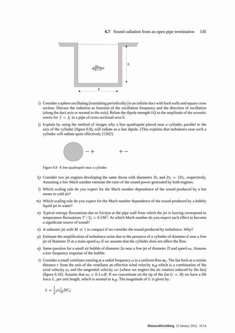
6.7 Sound radiation from an open pipe termination 145
h
h
i) Consider a sphere oscillating (translating periodically) in an infinite duct with hard walls and square crosssection. Discuss the radiation as function of the oscillation frequency and the direction of oscillation(along the duct axis or normal to the axis). Relate the dipolestrengthδQ to the amplitude of the acousticwaves for f < fc in a pipe of cross sectional areaS.
j) Explain by using the method of images why a line quadrupoleplaced near a cylinder, parallel to theaxis of the cylinder (figure 6.9), will radiate as a line dipole. (This explains that turbulence near such acylinder will radiate quite effectively [130]!)
Figure 6.9 A line quadrupole near a cylinder.
k) Consider two jet engines developing the same thrust with diametersD1 and D2 = 2D1, respectively.Assuming a low Mach number estimate the ratio of the sound power generated by both engines.
l) Which scaling rule do you expect for the Mach number dependence of the sound produced by a hotsteam in cold air?
m) Which scaling rule do you expect for the Mach number dependence of the sound produced by a bubblyliquid jet in water?
n) Typical entropy fluctuations due to friction at the pipe wall from which the jet is leaving correspond totemperature fluctuationsT ′/T0 ' 0.2M2. At which Mach number do you expect such effect to becomea significant source of sound?
o) A subsonic jet withM � 1 is compact if we consider the sound produced by turbulence.Why?
p) Estimate the amplification of turbulence noise due to the presence of a cylinder of diameterd near a freejet of diameterD at a main speedu0 if we assume that the cylinder does not affect the flow.
q) Same question for a small air bubble of diameter 2a near a free jet of diameterD and speedu0. Assumea low frequency response of the bubble.
r) Consider a small ventilator rotating at a radial frequencyω in a uniform flowu0. The fan feels at a certaindistancer from the axis of the ventilator an effective wind velocityveff which is a combination of theaxial velocityu0 and the tangential velocityωr (where we neglect the air rotation induced by the fan)(figure 6.10). Assume thatu0 = 0.1ωR. If we concentrate on the tip of the fan (r = R) we have a liftforceL, per unit length, which is normal toveff. The magnitude ofL is given by:
L = 1
2ρv2
effDCL
RienstraHirschberg 22 January 2012, 10:14
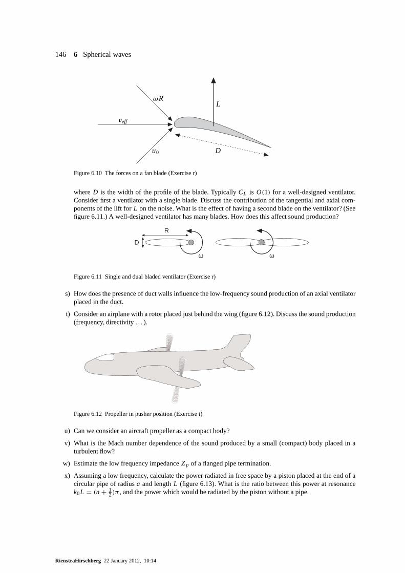
146 6 Spherical waves
u0
ωR
veff
L
D
Figure 6.10 The forces on a fan blade (Exercise r)
whereD is the width of the profile of the blade. TypicallyCL is O(1) for a well-designed ventilator.Consider first a ventilator with a single blade. Discuss the contribution of the tangential and axial com-ponents of the lift forL on the noise. What is the effect of having a second blade on theventilator? (Seefigure 6.11.) A well-designed ventilator has many blades. How does this affect sound production?
D
R
ω ω
Figure 6.11 Single and dual bladed ventilator (Exercise r)
s) How does the presence of duct walls influence the low-frequency sound production of an axial ventilatorplaced in the duct.
t) Consider an airplane with a rotor placed just behind the wing (figure 6.12). Discuss the sound production(frequency, directivity . . . ).
Figure 6.12 Propeller in pusher position (Exercise t)
u) Can we consider an aircraft propeller as a compact body?
v) What is the Mach number dependence of the sound produced bya small (compact) body placed in aturbulent flow?
w) Estimate the low frequency impedanceZp of a flanged pipe termination.
x) Assuming a low frequency, calculate the power radiated infree space by a piston placed at the end of acircular pipe of radiusa and lengthL (figure 6.13). What is the ratio between this power at resonancek0L = (n + 1
2)π , and the power which would be radiated by the piston without apipe.
RienstraHirschberg 22 January 2012, 10:14
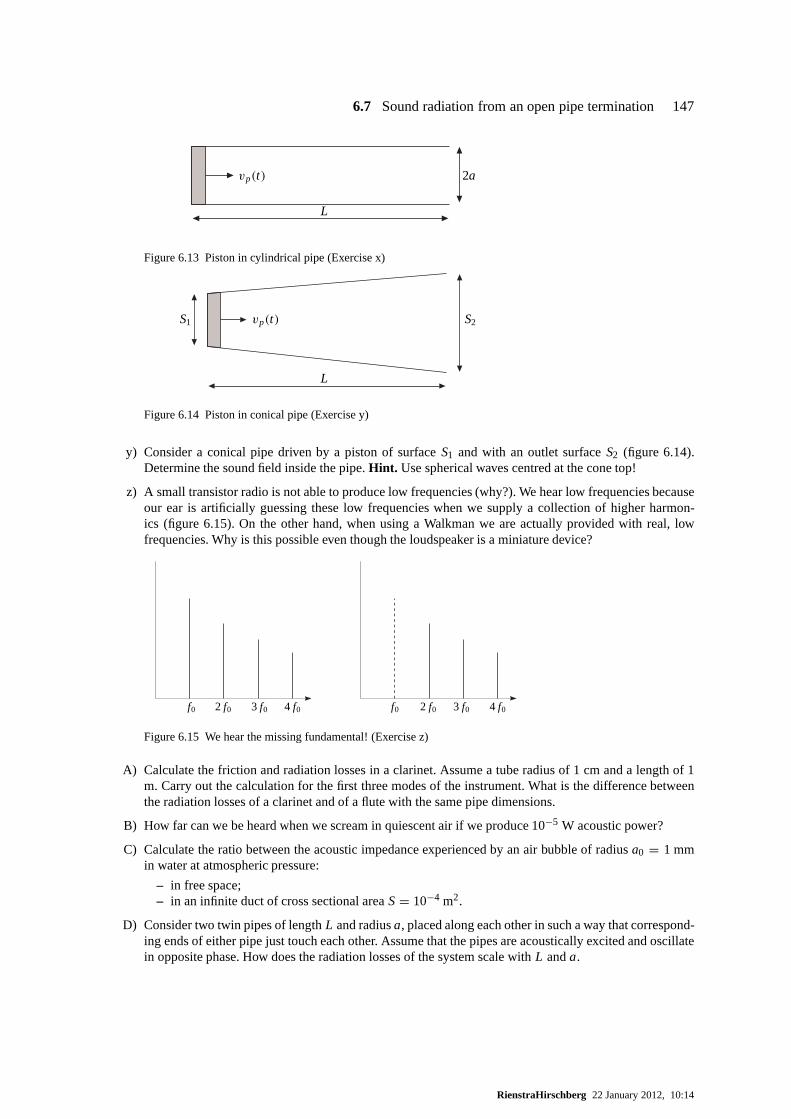
6.7 Sound radiation from an open pipe termination 147
vp(t)
L
2a
Figure 6.13 Piston in cylindrical pipe (Exercise x)
vp(t)
L
S1 S2
Figure 6.14 Piston in conical pipe (Exercise y)
y) Consider a conical pipe driven by a piston of surfaceS1 and with an outlet surfaceS2 (figure 6.14).Determine the sound field inside the pipe.Hint. Use spherical waves centred at the cone top!
z) A small transistor radio is not able to produce low frequencies (why?). We hear low frequencies becauseour ear is artificially guessing these low frequencies when we supply a collection of higher harmon-ics (figure 6.15). On the other hand, when using a Walkman we are actually provided with real, lowfrequencies. Why is this possible even though the loudspeaker is a miniature device?
f0 2 f0 3 f0 4 f0 f0 2 f0 3 f0 4 f0
Figure 6.15 We hear the missing fundamental! (Exercise z)
A) Calculate the friction and radiation losses in a clarinet. Assume a tube radius of 1 cm and a length of 1m. Carry out the calculation for the first three modes of the instrument. What is the difference betweenthe radiation losses of a clarinet and of a flute with the same pipe dimensions.
B) How far can we be heard when we scream in quiescent air if we produce 10−5 W acoustic power?
C) Calculate the ratio between the acoustic impedance experienced by an air bubble of radiusa0 = 1 mmin water at atmospheric pressure:
– in free space;– in an infinite duct of cross sectional areaS= 10−4 m2.
D) Consider two twin pipes of lengthL and radiusa, placed along each other in such a way that correspond-ing ends of either pipe just touch each other. Assume that thepipes are acoustically excited and oscillatein opposite phase. How does the radiation losses of the system scale withL anda.
RienstraHirschberg 22 January 2012, 10:14

7 Duct acoustics
In a duct of constant cross section the reduced wave (or Helmholtz) equation may be solved by meansof a series expansion in a particular family of solutions, called modes. They are related to the eigenso-lutions of the two-dimensional Laplace operator acting on across section. Therefore, the terminologyof modes contains many references to the corresponding eigenvalues.
Modes are interesting mathematically because they form, ingeneral, a complete basis by which anysolution can be represented. Physically, modes are interesting because they are solutions in their ownright, not just mathematical building blocks, and by their simple structure the usually complicatedbehaviour of the total field is more easily understood.
7.1 General formulation
The time-harmonic sound field in a duct of constant cross section with linear boundary conditionsthat are independent of the axial coordinate may be described by an infinite sum of special solutions,called modes, that retain their shape when travelling down the duct. They consist of an exponentialterm multiplied by the eigenfunctions of the Laplace operator corresponding to a duct cross section.
DA
∂A
n
x
y
z
Figure 7.1 A ductD of cross sectionA.
Consider the two-dimensional areaA with a smooth boundary∂A and an externally directed unitnormal n. For physical relevanceA should be simply connected, otherwise we would have severalindependent ducts. When we consider, for definiteness, thisarea be part of they, z-plane, it describesthe ductD (see Fig. 7.1) given by
D = {(x, y, z)|(y, z) ∈ A} (7.1)
with axial cross sections being copies ofA and where the normal vectorsn are the same for allx. Inthe usual complex notation (with+iωt–sign convention), the acoustic field
p(x, t) ≡ p(x, ω)eiωt , v(x, t) ≡ v(x, ω)eiωt (7.2)
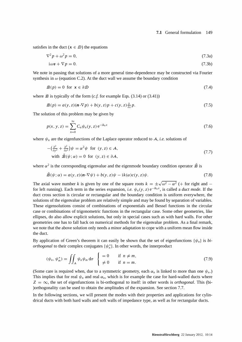
7.1 General formulation 149
satisfies in the duct (x ∈ D) the equations
∇2 p + ω2p = 0, (7.3a)
iωv + ∇ p = 0. (7.3b)
We note in passing that solutions of a more general time-dependence may be constructed via Fouriersynthesis inω (equation C.2). At the duct wall we assume the boundary condition
B(p) = 0 for x ∈ ∂D (7.4)
whereB is typically of the form (c.f. for example Eqs. (3.14) or (3.41))
B(p) = a(y, z)(n·∇ p)+ b(y, z)p + c(y, z) ∂∂x p. (7.5)
The solution of this problem may be given by
p(x, y, z) =∞∑
n=0
Cnψn(y, z)e−iknx (7.6)
whereψn are the eigenfunctions of the Laplace operator reduced toA, i.e.solutions of
−(∂2
∂y2 + ∂2
∂z2
)ψ = α2ψ for (y, z) ∈ A,
with B(ψ;α) = 0 for (y, z) ∈ ∂A,(7.7)
whereα2 is the corresponding eigenvalue and the eigenmode boundarycondition operatorB is
B(ψ;α) = a(y, z)(n·∇ψ)+ b(y, z)ψ − i k(α)c(y, z)ψ. (7.8)
The axial wave numberk is given by one of the square rootsk = ±√ω2 − α2 (+ for right and−
for left running). Each term in the series expansion,i.e.ψn(y, z)e−iknx, is called aduct mode. If theduct cross section is circular or rectangular and the boundary condition is uniform everywhere, thesolutions of the eigenvalue problem are relatively simple and may be found by separation of variables.These eigensolutions consist of combinations of exponentials and Bessel functions in the circularcase or combinations of trigonometric functions in the rectangular case. Some other geometries, likeellipses, do also allow explicit solutions, but only in special cases such as with hard walls. For othergeometries one has to fall back on numerical methods for the eigenvalue problem. As a final remark,we note that the above solution only needs a minor adaptationto cope with a uniform mean flow insidethe duct.
By application of Green’s theorem it can easily be shown thatthe set of eigenfunctions{ψn} is bi-orthogonalto their complex conjugates{ψ∗
n}. In other words, the innerproduct
(ψn, ψ∗m) =
∫∫
A
ψnψm dσ
{= 0 if n 6= m,
6= 0 if n = m.(7.9)
(Some care is required when, due to a symmetric geometry, each αn is linked to more than oneψn.)This implies that for realψn and realαn, which is for example the case for hard-walled ducts whereZ = ∞, the set of eigenfunctions is bi-orthogonal to itself: in other words isorthogonal. This (bi-)orthogonality can be used to obtain the amplitudes of the expansion. See section 7.7.
In the following sections, we will present the modes with their properties and applications for cylin-drical ducts with both hard walls and soft walls of impedancetype, as well as for rectangular ducts.
RienstraHirschberg 22 January 2012, 10:14
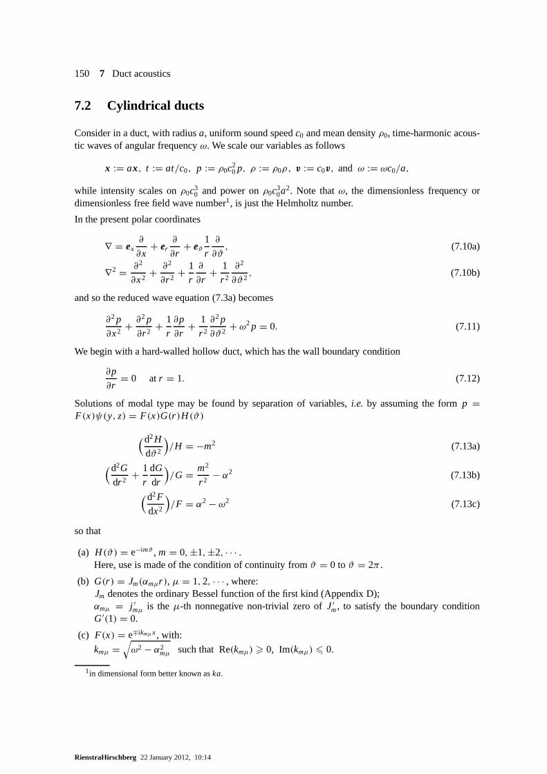
150 7 Duct acoustics
7.2 Cylindrical ducts
Consider in a duct, with radiusa, uniform sound speedc0 and mean densityρ0, time-harmonic acous-tic waves of angular frequencyω. We scale our variables as follows
x := ax, t := at/c0, p := ρ0c20 p, ρ := ρ0ρ, v := c0v, and ω := ωc0/a,
while intensity scales onρ0c30 and power onρ0c3
0a2. Note thatω, the dimensionless frequency ordimensionless free field wave number1, is just the Helmholtz number.
In the present polar coordinates
∇ = ex∂
∂x+ er
∂
∂r+ eϑ
1
r
∂
∂ϑ, (7.10a)
∇2 = ∂2
∂x2+ ∂2
∂r 2+ 1
r
∂
∂r+ 1
r 2
∂2
∂ϑ2, (7.10b)
and so the reduced wave equation (7.3a) becomes
∂2p
∂x2+ ∂2 p
∂r 2+ 1
r
∂p
∂r+ 1
r 2
∂2p
∂ϑ2+ ω2p = 0. (7.11)
We begin with a hard-walled hollow duct, which has the wall boundary condition
∂p
∂r= 0 atr = 1. (7.12)
Solutions of modal type may be found by separation of variables, i.e. by assuming the formp =F(x)ψ(y, z) = F(x)G(r )H (ϑ)
(d2H
dϑ2
)/H = −m2 (7.13a)
(d2G
dr 2+ 1
r
dG
dr
)/G = m2
r 2− α2 (7.13b)
(d2F
dx2
)/F = α2 − ω2 (7.13c)
so that
(a) H (ϑ) = e−imϑ , m = 0,±1,±2, · · · .Here, use is made of the condition of continuity fromϑ = 0 toϑ = 2π .
(b) G(r ) = Jm(αmµr ), µ = 1,2, · · · , where:Jm denotes the ordinary Bessel function of the first kind (Appendix D);αmµ = j ′
mµ is theµ-th nonnegative non-trivial zero ofJ ′m, to satisfy the boundary condition
G′(1) = 0.
(c) F(x) = e∓ikmµx, with:
kmµ =√ω2 − α2
mµ such that Re(kmµ) > 0, Im(kmµ) 6 0.
1in dimensional form better known aska.
RienstraHirschberg 22 January 2012, 10:14

7.2 Cylindrical ducts 151
Although technically speaking{α2m,µ} are the eigenvalues of (minus) the cross-sectional Laplaceop-
erator, it is common practice to refer toαmµ as the radial eigenvalue or radial modal wave number, tom as the circumferential eigenvalue or circumferential wavenumber, and tokmµ as the axial eigen-value or axial wave number. The associated solutions are called duct modes, and they form a completeset of building blocks suitable for constructing any sound field in a duct. At the same time, they areparticular shape-preserving solutions with easily interpretable properties.
Note that allαmµ andm are real, while only a finite number ofkmµ are real; see figure 7.2). The branch
-15
-10
-5
0
5
10
15
-8 -6 -4 -2 0 2 4 6 8
k05
k04
k03
k02 k01
−k05
−k04
−k03
−k02−k01
Figure 7.2 Complex axial wave numbers (m = 0,ω = 5).
we selected here of the complex square rootkmµ is such thate−ikmµx describes a right-running waveandeikmµx a left-running wave. This will be further clarified later.
These modes (normalized for convenience)
pmµ(x, r, ϑ) = Umµ(r )e−imϑ∓ikmµx, (7.14)
Umµ(r ) = Nmµ Jm(αmµr ),
Nmµ ={
12(1 − m2/α2
mµ)Jm(αmµ)2}−1/2
,
form (for fixed x) a complete set (inL2-norm over(r, ϑ)), so by superposition we can write anysolution as the following modal expansion:
p(x, r, ϑ) =∞∑
m=−∞
∞∑
µ=1
(Amµ e−ikmµx +Bmµ eikmµx)Umµ(r )e−imϑ .
(7.15)
The normalization factorNmµ is chosen such that a modal amplitudeAmµ scales with the energycontent of the corresponding mode (see below).
A surface of constant phase,i.e. mϑ + Re(kmµ)x = constant, is a helix of pitch 2πm/Re(kmµ); seefigure 7.3.
RienstraHirschberg 22 January 2012, 10:14

152 7 Duct acoustics
x-axis
Figure 7.3 Surface of constant phasemϑ + Re(kmµ)x.
An important special case is the plane wavem = 0,µ = 1, with
j ′01 = 0, α01 = 0, k01 = ω, N01 =
√2, p01 =
√2e−iωx .
In fact, this is the only non-trivial eigenvalue equal to zero. All others are greater, the smallest beinggiven by
j ′11 = 1.84118· · · .
Since the zeros ofJ ′m form an ever increasing sequence both inm and inµ (with j ′
mµ ' (µ+ 12m− 1
4)π
for µ → ∞) (see Appendix D), there are for anyω always a (finite)µ = µ0 andm = m0 beyondwhichα2
mµ > ω2, so thatkmµ is purely imaginary, and the mode decays exponentially inx.
So we see that there are always afinitenumber of modes withreal kmµ (see figure 7.2). Since they arethe only modes that propagate (see below), they are calledcut-on. The remaining infinite number ofmodes, withimaginary kmµ, are evanescent and therefore calledcut-off. This cut-on and cut-off modesare essentially similar to the radiating and evanescent waves discussed in section 3.3.
For low frequency,i.e. for
ω < j ′11 = 1.84118· · ·
all modes are cut-off except for the plane wave. In this case aplane wave approximation (i.e.consider-ing only the first mode) is applicable if we are far enough awayfrom any sources, changes in boundarycondition, or other scattering objects, for the generated evanescent modes to become negligible.
From the orthogonality relation2 of equation 7.9 (note that we have here a hard-walled duct)∫ 1
0
∫ 2π
0Umµ(r )e−imϑ
(Unν(r )e−inϑ
)∗r dϑdr = 2πδmnδµν (7.16)
we find by integration of the time-averaged axial intensity
〈I · ex〉 = 14(pu∗ + p∗u) = 1
2 Re(pu∗)
over a duct cross sectionx = constant the transmitted acoustic power
P = π
ω
∞∑
m=−∞
∞∑
µ=1
Re(kmµ)(|Amµ|2 − |Bmµ|2)+ 2 Im(kmµ) Im(A∗
mµBmµ)
. (7.17)
2 δi j = 1 if i = j , δi j = 0 if i 6= j
RienstraHirschberg 22 January 2012, 10:14
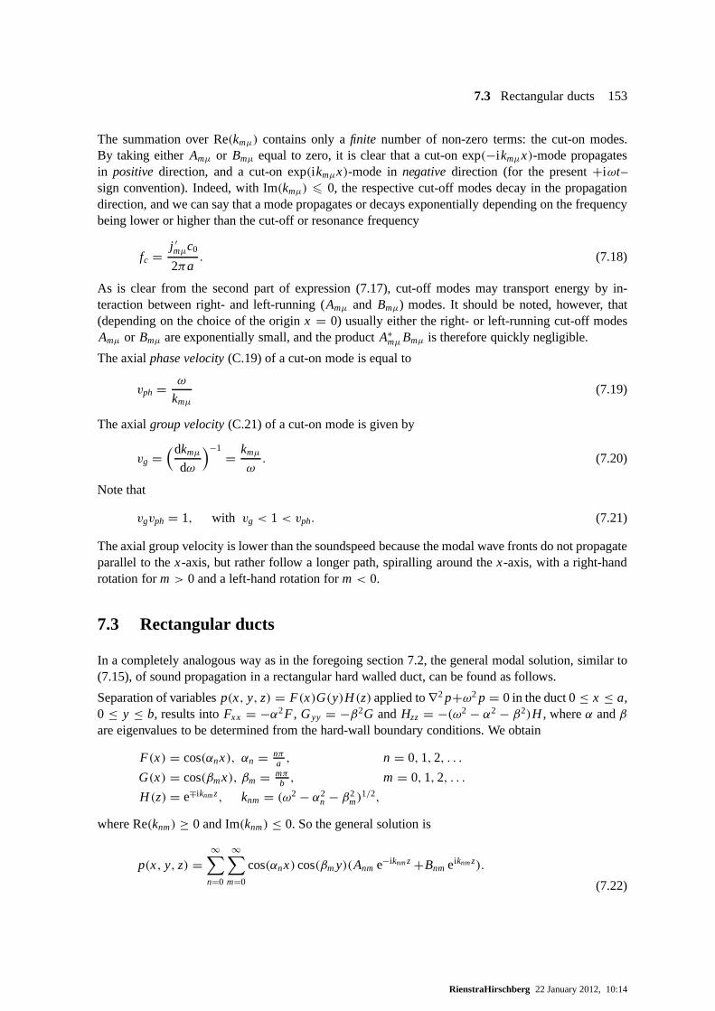
7.3 Rectangular ducts 153
The summation over Re(kmµ) contains only afinite number of non-zero terms: the cut-on modes.By taking eitherAmµ or Bmµ equal to zero, it is clear that a cut-on exp(−i kmµx)-mode propagatesin positivedirection, and a cut-on exp(i kmµx)-mode innegativedirection (for the present+iωt–sign convention). Indeed, with Im(kmµ) 6 0, the respective cut-off modes decay in the propagationdirection, and we can say that a mode propagates or decays exponentially depending on the frequencybeing lower or higher than the cut-off or resonance frequency
fc =j ′mµc0
2πa. (7.18)
As is clear from the second part of expression (7.17), cut-off modes may transport energy by in-teraction between right- and left-running (Amµ and Bmµ) modes. It should be noted, however, that(depending on the choice of the originx = 0) usually either the right- or left-running cut-off modesAmµ or Bmµ are exponentially small, and the productA∗
mµBmµ is therefore quickly negligible.
The axialphase velocity(C.19) of a cut-on mode is equal to
vph = ω
kmµ(7.19)
The axialgroup velocity(C.21) of a cut-on mode is given by
vg =(dkmµ
dω
)−1= kmµ
ω. (7.20)
Note that
vgvph = 1, with vg < 1< vph. (7.21)
The axial group velocity is lower than the soundspeed because the modal wave fronts do not propagateparallel to thex-axis, but rather follow a longer path, spiralling around the x-axis, with a right-handrotation form> 0 and a left-hand rotation form< 0.
7.3 Rectangular ducts
In a completely analogous way as in the foregoing section 7.2, the general modal solution, similar to(7.15), of sound propagation in a rectangular hard walled duct, can be found as follows.
Separation of variablesp(x, y, z) = F(x)G(y)H (z) applied to∇2 p+ω2 p = 0 in the duct 0≤ x ≤ a,0 ≤ y ≤ b, results intoFxx = −α2F , Gyy = −β2G andHzz = −(ω2 − α2 − β2)H , whereα andβare eigenvalues to be determined from the hard-wall boundary conditions. We obtain
F(x) = cos(αnx), αn = nπa , n = 0,1,2, . . .
G(x) = cos(βmx), βm = mπb , m = 0,1,2, . . .
H (z) = e∓iknmz, knm = (ω2 − α2n − β2
m)1/2,
where Re(knm) ≥ 0 and Im(knm) ≤ 0. So the general solution is
p(x, y, z) =∞∑
n=0
∞∑
m=0
cos(αnx) cos(βmy)(Anm e−iknmz +Bnm eiknmz).
(7.22)
RienstraHirschberg 22 January 2012, 10:14
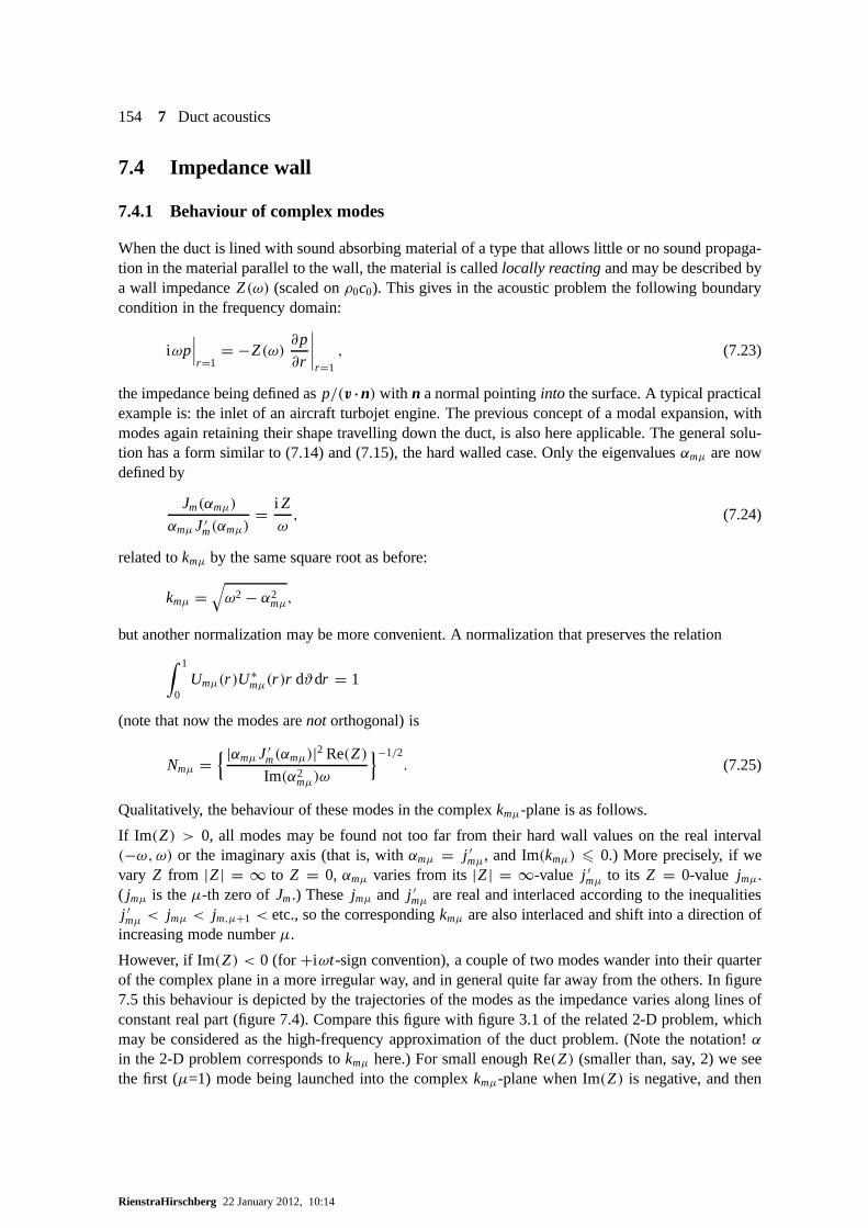
154 7 Duct acoustics
7.4 Impedance wall
7.4.1 Behaviour of complex modes
When the duct is lined with sound absorbing material of a typethat allows little or no sound propaga-tion in the material parallel to the wall, the material is called locally reactingand may be described bya wall impedanceZ(ω) (scaled onρ0c0). This gives in the acoustic problem the following boundarycondition in the frequency domain:
iωp∣∣∣r=1
= −Z(ω)∂p
∂r
∣∣∣∣r=1
, (7.23)
the impedance being defined asp/(v ·n) with n a normal pointinginto the surface. A typical practicalexample is: the inlet of an aircraft turbojet engine. The previous concept of a modal expansion, withmodes again retaining their shape travelling down the duct,is also here applicable. The general solu-tion has a form similar to (7.14) and (7.15), the hard walled case. Only the eigenvaluesαmµ are nowdefined by
Jm(αmµ)
αmµJ ′m(αmµ)
= i Z
ω, (7.24)
related tokmµ by the same square root as before:
kmµ =√ω2 − α2
mµ,
but another normalization may be more convenient. A normalization that preserves the relation
∫ 1
0Umµ(r )U
∗mµ(r )r dϑdr = 1
(note that now the modes arenot orthogonal) is
Nmµ ={ |αmµJ ′
m(αmµ)|2 Re(Z)
Im(α2mµ)ω
}−1/2. (7.25)
Qualitatively, the behaviour of these modes in the complexkmµ-plane is as follows.
If Im (Z) > 0, all modes may be found not too far from their hard wall values on the real interval(−ω,ω) or the imaginary axis (that is, withαmµ = j ′
mµ, and Im(kmµ) 6 0.) More precisely, if wevary Z from |Z| = ∞ to Z = 0, αmµ varies from its|Z| = ∞-value j ′
mµ to its Z = 0-value jmµ.( jmµ is theµ-th zero ofJm.) Thesejmµ and j ′
mµ are real and interlaced according to the inequalitiesj ′mµ < jmµ < jm,µ+1 < etc., so the correspondingkmµ are also interlaced and shift into a direction of
increasing mode numberµ.
However, if Im(Z) < 0 (for +iωt-sign convention), a couple of two modes wander into their quarterof the complex plane in a more irregular way, and in general quite far away from the others. In figure7.5 this behaviour is depicted by the trajectories of the modes as the impedance varies along lines ofconstant real part (figure 7.4). Compare this figure with figure 3.1 of the related 2-D problem, whichmay be considered as the high-frequency approximation of the duct problem. (Note the notation!αin the 2-D problem corresponds tokmµ here.) For small enough Re(Z) (smaller than, say, 2) we seethe first (µ=1) mode being launched into the complexkmµ-plane when Im(Z) is negative, and then
RienstraHirschberg 22 January 2012, 10:14

7.4 Impedance wall 155
6
real axis
imaginaryaxis Re(Z) =constant
Z ∈ C
Figure 7.4 Complex impedance plane.
returning as a (for example)µ=4 or 2 mode when Im(Z) is positive. We will call these irregular modessurface waves: their maximum is at the wall surface, and away from the wall they decay exponentially([189]). This is most purely the case for an imaginary impedanceZ = i X. See figure 7.6.
A solutionαmµ = i%mµ, %mµ real, may be found3 satisfying
Im(%mµ)
%mµ I ′m(%mµ)
= − X
ωif − ω
m< X < 0. (7.26)
The modal shape inr , described byJm(αmµr ) = i mIm(%mµr ), is exponentially restricted to the imme-diate neighbourhood ofr = 1 and indeed shows the surface wave character, since the modified Besselfunction Im(x) has exponential behaviour forx → ∞. It is interesting to note that the correspondingaxial wave numberkmµ = (ω2 + %2
mµ)1/2 is now larger thanω. Hence, the modal phase velocity is
smaller than the sound speed, which is indeed to be expected for anon-radiatingsurface wave. Thegroup velocity (7.20) depends onZ(ω).
7.4.2 Attenuation
Usually, lining is applied to reduce the sound level by dissipation. It is a simple exercise to verify thatthe time-averaged intensity at the wall directed into the wall ( i.e. the dissipated power density) of amode is
〈I ·er 〉 ∝ Im(α2mµ). (7.27)
A natural practical question is then: which impedanceZ gives the greatest reduction. This questionhas, however, many answers. In general, the optimum will depend on the source of the sound. Ifmore than one frequency contributes, we have to include the way Z = Z(ω) depends onω. Alsothe geometry may play a rôle. Although it is strictly speaking not dissipation, the net reduction maybenefit from reflections at discontinuities in the duct (hard/soft walls, varying cross section).
A simple approach would be to look at the reduction per mode, and to maximize the decay rate ofthe least attenuated mode,i.e. the one with thesmallest| Im(kmµ)|. A further simplification is basedon the observation that the decay rate Im(kmµ) of a mode increases with increasing order, so that a(relatively) large decay rate is obtained if the first and second mode (of the most relevantm) coalesce(Cremer’s optimum). This is obtained if also the derivativeto αmµ of (7.24) vanishes, yielding theadditional condition
J ′m(αmµ)
2 +(1 − m2
α2mµ
)Jm(αmµ)
2 = 0 (7.28)
3The functionh(z) = z I′m(z)/Im(z) increases monotonically inz, with h(0) = m, andh(z) ∼ z asz → ∞.
RienstraHirschberg 22 January 2012, 10:14
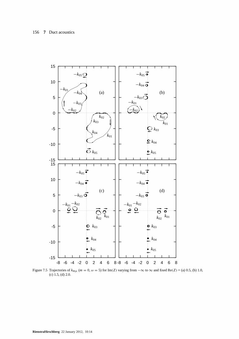
156 7 Duct acoustics
-15
-10
-5
0
5
10
15
-15
-10
-5
0
5
10
15
-8 -6 -4 -2 0 2 4 6 8 -8 -6 -4 -2 0 2 4 6 8
(a)
k01
k02k03
k04
k05
−k01
−k02
−k03
−k04
−k05
6
?
-
�
(b)
k01
k02
k03
k04
k05
−k01
−k02
−k03
−k04
−k05
AAU
AAK
-
-
-
�
�
�
(c)
k01k02
k03
k04
k05
−k01−k02
−k03
−k04
−k05
- -��
-
-
-
�
�
�
(d)
k01k02
k03
k04
k05
−k01−k02
−k03
−k04
−k05
- -��
-
-
-
�
�
�
Figure 7.5 Trajectories ofkmµ (m = 0,ω = 5) for Im(Z) varying from−∞ to ∞ and fixed Re(Z) = (a) 0.5, (b) 1.0,(c) 1.5, (d) 2.0.
RienstraHirschberg 22 January 2012, 10:14
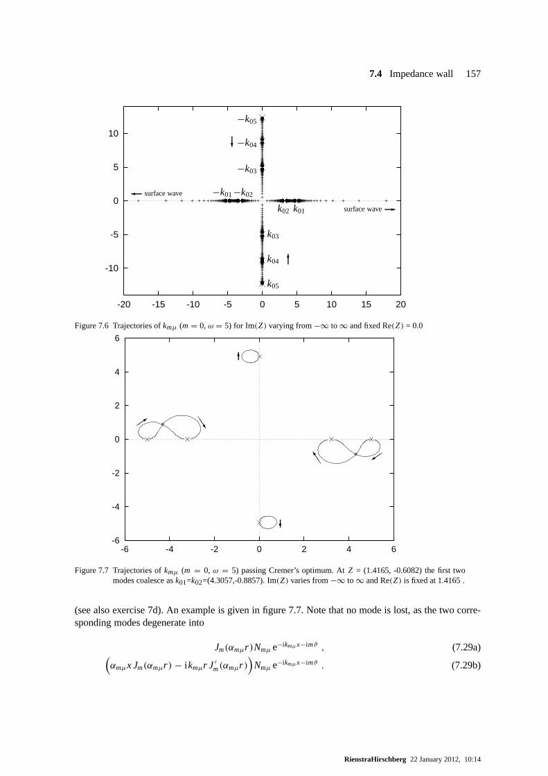
7.4 Impedance wall 157
-10
-5
0
5
10
-20 -15 -10 -5 0 5 10 15 20
k05
k04
k03
k02 k01
−k05
−k04
−k03
−k02−k01
-surface wave
� surface wave
6
?
Figure 7.6 Trajectories ofkmµ (m = 0,ω = 5) for Im(Z) varying from−∞ to ∞ and fixed Re(Z) = 0.0
-6
-4
-2
0
2
4
6
-6 -4 -2 0 2 4 6
°
°
��3
��+
JJ
JJ]
6
?
Figure 7.7 Trajectories ofkmµ (m = 0, ω = 5) passing Cremer’s optimum. AtZ = (1.4165, -0.6082) the first twomodes coalesce ask01=k02=(4.3057,-0.8857). Im(Z) varies from−∞ to ∞ and Re(Z) is fixed at 1.4165 .
(see also exercise 7d). An example is given in figure 7.7. Notethat no mode is lost, as the two corre-sponding modes degenerate into
Jm(αmµr )Nmµ e−ikmµx−imϑ , (7.29a)(αmµx Jm(αmµr )− i kmµr J ′
m(αmµr ))
Nmµ e−ikmµx−imϑ . (7.29b)
RienstraHirschberg 22 January 2012, 10:14
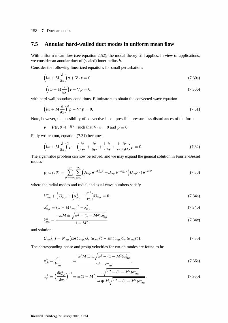
158 7 Duct acoustics
7.5 Annular hard-walled duct modes in uniform mean flow
With uniform mean flow (see equation 2.52), the modal theory still applies. In view of applications,we consider an annular duct of (scaled) inner radiush.
Consider the following linearized equations for small perturbations(iω + M
∂
∂x
)p + ∇ ·v = 0, (7.30a)
(iω + M
∂
∂x
)v + ∇ p = 0, (7.30b)
with hard-wall boundary conditions. Eliminatev to obtain the convected wave equation(iω + M
∂
∂x
)2p − ∇2 p = 0, (7.31)
Note, however, the possibility of convective incompressible pressureless disturbances of the form
v = F(r, θ)e−i ωM x, such that∇ ·v = 0 andp ≡ 0.
Fully written out, equation (7.31) becomes
(iω + M
∂
∂x
)2p −
( ∂2
∂x2+ ∂2
∂r 2+ 1
r
∂
∂r+ 1
r 2
∂2
∂ϑ2
)p = 0. (7.32)
The eigenvalue problem can now be solved, and we may expand the general solution in Fourier-Besselmodes
p(x, r, θ) =∞∑
m=−∞
∞∑
µ=1
(Amµ e−ik+
mµx +Bmµ e−ik−mµx
)Umµ(r )e−imθ (7.33)
where the radial modes and radial and axial wave numbers satisfy
U ′′mµ + 1
rU ′
mµ +(α2
mµ − m2
r 2
)Umµ = 0 (7.34a)
α2mµ = (ω − Mkmµ)
2 − k2mµ (7.34b)
k±mµ =
−ωM ±√ω2 − (1 − M2)α2
mµ
1 − M2(7.34c)
and solution
Umµ(r ) = Nmµ
(cos(τmµ)Jm(αmµr )− sin(τmµ)Ym(αmµr )
). (7.35)
The corresponding phase and group velocities for cut-on modes are found to be
v±ph = ω
k±mµ
=ω2M ± ω
√ω2 − (1 − M2)α2
mµ
ω2 − α2mµ
, (7.36a)
v±g =
(dk±mµ
dω
)−1= ±(1 − M2)
√ω2 − (1 − M2)α2
mµ
ω ∓ M√ω2 − (1 − M2)α2
mµ
. (7.36b)
RienstraHirschberg 22 January 2012, 10:14
7.5 Annular hard-walled duct modes in uniform mean flow 159
Due to the mean flow, the axial modal wave numbers are shifted to the left (M > 0), or right (M < 0),by a fixed amount of−ωM/(1 − M2), while the (dimensionless) cut-off frequency is lowered fromω = αmµ for no flow toω = αmµ
√1 − M2 with flow. So with flow more modes are possibly cut-on
than without. Note that (forM > 0) the rightrunning modes that become cut-on in this way (andonly these) have a negative real part of their axial wave number. Indeed, rightrunning modes with afrequency along the interval
αmµ
√1 − M2 < ω < αmµ
have phase velocities that areoppositeto their group velocities, the speed of information. The sameapplies for left-running modes ifM < 0. Sincev+
g > 0 andv−g < 0, this shows that it is not the sign
of kmµ but of its radical that corresponds with the direction of propagation [138];c.f. equation (7.42).
Eigenvaluesαmµ are determined via boundary conditionU ′mµ(1) = U ′
mµ(h) = 0
J ′m(α)Y
′m(αh)− J ′
m(αh)Y′m(α) = 0 (7.37)
The normalization is such that∫ 1
h U2(r )r dr = 1 (c.f. [188]), so
Nmµ =12
√2παmµ
{1 − m2/α2
mµ
J ′m(αmµ)2 + Y′
m(αmµ)2−
1 − m2/α2mµh2
J ′m(αmµh)2 + Y′
m(αmµh)2
} 12
(7.38)
and
τmµ = arctan{ J ′
m(αmµ)
Y′m(αmµ)
}. (7.39)
This implies the following choice of signs
cosτmµ = sign(Y′m(αmµ))
Y′m(αmµ)√
J ′m(αmµ)2 + Y′
m(αmµ)2, (7.40a)
sinτmµ = sign(Y′m(αmµ))
J ′m(αmµ)√
J ′m(αmµ)2 + Y′
m(αmµ)2, (7.40b)
with the advantage that it reduces to the expected limitNmµ Jm(αmµr ) for h → 0. Other choices, forexample without the factor sign(Y′
m), are also possible.
The modes are physically interesting because their shape remains the same. Mathematically, they areinteresting because they form a complete and orthonormalL2-basis for the solutions of the convectedwave equation (except for the pressureless convected perturbations):
∫ 2π
0
∫ 1
hUmµ(r )Unν(r )eimθ e−inθ r dr dθ = 2πδmnδµν (7.41)
It is convenient to introduce theLorentzor Prandtl-Glauerttype transformation (see 3.45 and section9.1.1)
β =√
1 − M2, x = βX, ω = β�, αmµ = �γmµ
k±mµ = ±�σmµ −�M
β, σmµ =
√1 − γ 2
mµ,(7.42)
RienstraHirschberg 22 January 2012, 10:14
160 7 Duct acoustics
whereσmµ is positive real or negative imaginary, then we have for pressure p and axial acousticvelocity v
p =∞∑
m=−∞
∞∑
µ=1
(Amµ e−i�σmµX +Bmµ ei�σmµX
)ei�M X Umµ(r )e−imθ (7.43a)
v =∞∑
m=−∞
∞∑
µ=1
( σmµ − M
1 − MσmµAmµ e−i�σmµX − σmµ + M
1 + MσmµBmµ ei�σmµX
)ei�M X Umµ(r )e−imθ
(7.43b)
This includes the important case of the plane wavem = 0,µ = 1, with α01 = 0, k±01 = ±ω/(1 ± M)
andU01 = (2/(1 − h2))1/2, such that
p(x, r, θ) =[
A01 e− iωx1+M +B01e
iωx1−M
]( 2
1 − h2
)1/2, (7.44a)
v(x, r, θ) =[
A01 e− iωx1+M −B01e
iωx1−M
]( 2
1 − h2
)1/2. (7.44b)
If we have at positionx = 0 a given pressure and axial velocity profilesP(0, r, θ) andV(0, r, θ), wecan expand these profiles in the following Fourier-Bessel series
P(0, r, θ) =∞∑
m=−∞
∞∑
µ=1
PmµUmµ(r )e−imθ , (7.45a)
V(0, r, θ) =∞∑
m=−∞
∞∑
µ=1
VmµUmµ(r )e−imθ , (7.45b)
where
Pmµ = 1
2π
∫ 2π
0
∫ 1
hP(0, r, θ)Umµ(r )eimθ r dr dθ, (7.46a)
Vmµ = 1
2π
∫ 2π
0
∫ 1
hV(0, r, θ)Umµ(r )eimθ r dr dθ. (7.46b)
If these pressure and velocity profiles satisfy the above propagation model of sound in uniform meanflow, the corresponding amplitudesAmµ andBmµ are found from identifying
Pmµ = Amµ + Bmµ, (7.47a)
Vmµ = σmµ − M
1 − MσmµAmµ − σmµ + M
1 + MσmµBmµ, (7.47b)
leading to
Amµ =(1 − Mσmµ)(σmµ + M)Pmµ + (1 − M2σ 2
mµ)Vmµ
2σmµ(1 − M2), (7.48a)
Bmµ =(1 + Mσmµ)(σmµ − M)Pmµ − (1 − M2σ 2
mµ)Vmµ
2σmµ(1 − M2). (7.48b)
RienstraHirschberg 22 January 2012, 10:14
7.6 Behaviour of soft-wall modes and mean flow 161
From the axial intensity in hard-walled flow duct
〈I x〉 = 12 Re
[(p + Mu)(u∗ + Mp∗)
](7.49)
we obtain the axial power:
P = πβ4∞∑
m=−∞
µ0∑
µ=1
σmµ
[ |Amµ|2(1 − Mσmµ)2
− |Bmµ|2(1 + Mσmµ)2
]+
+ 2πβ4∞∑
m=−∞
∞∑
µ=µ0+1
|σmµ|(1 + M2|σmµ|2)2
·[Im(AmµB∗
mµ)(1 − M2|σmµ|2) − Re(AmµB∗mµ)2M|σmµ|
](7.50)
whereµ0 is the number of cut-on modes. Note the coupling between left- and right-running cut-offmodes.
7.6 Behaviour of soft-wall modes and mean flow
Consider a cylindrical duct with soft wall of specific impedance Z and uniform mean flow of MachnumberM. For this configuration the acoustic field allows again modes, similar to the no-flow situa-tion, although their behaviour with respect to possible surface waves is more complicated [195].
We start with modes of the same form as for the hard wall case (equations 7.33 with 7.42, and 7.43a)for pressurep and radial velocityv
p = e−i�σ X+i�M X Jm(�γ r ), v = iβγ
1 − Mσe−i�σ X+i�M X J ′
m(�γ r ),
whereγ 2 + σ 2 = 1 and the sign selected ofσ depends (in general) on the direction of propagation.We dropped the exponentials with iωt and imθ . From the boundary condition (see equation 3.41)
iωZv =(iω + M ∂
∂x
)p
we find the equation for reduced axial wave numberσ for any givenZ, m, andω
(1 − Mσ )2Jm(�γ )− iβ3Zγ J ′m(�γ ) = 0. (7.51)
A graphical description of their behaviour as a function of Im Z (from +∞ down to−∞) and fixedReZ is given in the series of figures (7.8). For large enough frequency,ω, the behaviour of the modescan be classified as follows. Whenσ is near a hard-wall value, the mode described is really of acousticnature, extending radially through the whole duct. However, whenσ is far enough away from a hard-wall value, the imaginary part of�γ becomes significant. The complex Bessel functionJm(�γ r )becomes exponentially decaying away from the wall, and the mode is radially restricted to the ductwall region. In other words, it has become a surface wave, of two-dimensional nature, approximatelydescribed by the theory of section 3.2.6 (eqn. 3.46).
The “egg” (figure 3.3), indicating the location of possible surface waves in the 2D limit, is drawn inthe figures by a dotted line. The 2D surface wave solutions areindicated by black lines. The behaviourof the modes is to a certain extent similar to the no-flow situation (section 7.4.1, figures 7.5), althoughthe effect of the mean flow is that we have now 4 rather than 2 possible surface waves.
RienstraHirschberg 22 January 2012, 10:14
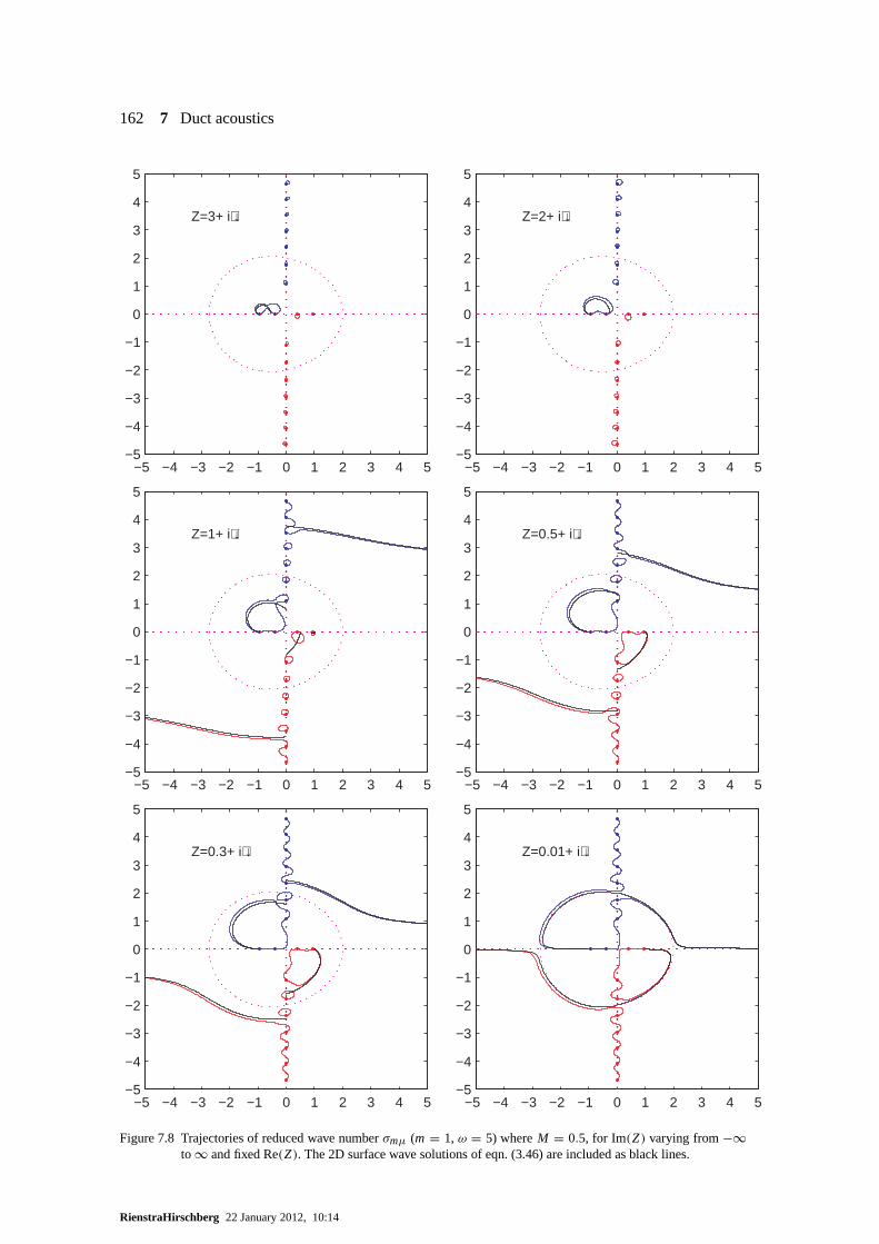
162 7 Duct acoustics
−5 −4 −3 −2 −1 0 1 2 3 4 5−5
−4
−3
−2
−1
0
1
2
3
4
5
Z=3+ i⋅↓
−5 −4 −3 −2 −1 0 1 2 3 4 5−5
−4
−3
−2
−1
0
1
2
3
4
5
Z=2+ i⋅↓
−5 −4 −3 −2 −1 0 1 2 3 4 5−5
−4
−3
−2
−1
0
1
2
3
4
5
Z=1+ i⋅↓
−5 −4 −3 −2 −1 0 1 2 3 4 5−5
−4
−3
−2
−1
0
1
2
3
4
5
Z=0.5+ i⋅↓
−5 −4 −3 −2 −1 0 1 2 3 4 5−5
−4
−3
−2
−1
0
1
2
3
4
5
Z=0.3+ i⋅↓
−5 −4 −3 −2 −1 0 1 2 3 4 5−5
−4
−3
−2
−1
0
1
2
3
4
5
Z=0.01+ i⋅↓
Figure 7.8 Trajectories of reduced wave numberσmµ (m = 1, ω = 5) whereM = 0.5, for Im(Z) varying from−∞to ∞ and fixed Re(Z). The 2D surface wave solutions of eqn. (3.46) are included asblack lines.
RienstraHirschberg 22 January 2012, 10:14
7.7 Source expansion 163
For large ReZ, the modes remain near their hard-wall values. For lower values of ReZ the behaviourbecomes more irregular. The modes change position with a neighbour, and some become temporarilya surface wave. The two hydrodynamic modes disappear to infinity for Im Z → −∞ like is describedin equation (3.47).
7.7 Source expansion
7.7.1 Modal amplitudes
A source atx = 0, defined by
p(x, r, ϑ)∣∣∣x=0
= p0(r, ϑ)
produces in a hard walled duct a sound field (7.15) with modal amplitudes given by (inx > 0)
Amµ = 1
2π
∫ 2π
0
∫ 1
0p0(r, ϑ)Umµ(r )eimϑ r dr dϑ (7.52a)
Bmµ = 0 (7.52b)
(use (7.16)), and the same inx < 0 but with A andB interchanged. Note that, similar to the evanes-cent waves of section 3.3, details of the source (averaged out for the lower modes in the process ofintegration), only contribute to higher order modes and do not generate sound if these modes arecut-off.
7.7.2 Rotating fan
Of practical interest, especially in aircraft noise reduction [229], is the following model of a propelleror fan with B identical blades, equally spaced1ϑ = 2π/B radians apart, rotating with angular speed�. If at some timet = 0 at a fixed positionx the field due to one blade is given by the shape functionq(ϑ, r ), then from periodicity the total field is described by
p(r, ϑ,0) = q(ϑ, r ) + q(ϑ −1ϑ, r )+ · · · + q(ϑ − (B − 1)1ϑ, r )
=B−1∑
k=0
q(ϑ − 2πk
B , r).
This function, periodic inϑ with period 2π/B, may be expanded in a Fourier series:
p(ϑ, r,0) =∞∑
n=−∞qn(r )e−inBϑ .
Since the field is associated to the rotor, it is a function ofϑ −�t . So at a timet
p(ϑ, r, t) =B−1∑
k=0
q(ϑ −�t − 2πk
B , r)
=∞∑
n=−∞qn(r )einB�t−inBϑ (7.53)
RienstraHirschberg 22 January 2012, 10:14
164 7 Duct acoustics
(with q−n = q∗n becausep is real). Evidently, the field is built up from harmonics of the blade passing
frequencyB�. Note that each frequencyω = nB� is now linked to a circumferential periodicitym = nB, and we jump with stepsB through the modalm-spectrum. Since the plane wave (m = 0) isgenerated with frequencyω = 0 it is acoustically not interesting, and we may ignore this component.An interesting consequence for a rotor in a duct is the observation that it is not obvious if there is(propagating) sound generated at all: the frequency must behigher than the cut-off frequency. For anyharmonic (n > 0) we have:
fm = m�
2π>
j ′m1c0
2πa(7.54)
which is for the tip Mach numberMtip the condition
Mtip = a�
c0>
j ′m1
m. (7.55)
Since the first zero ofJ ′m is always (slightly) larger thanm (Appendix D), it implies that the tip must
rotatesupersonically(Mtip > 1) for the fan to produce sound.
Of course, in practice a ducted fan with subsonically rotating blades will not be entirely silent. For ex-ample, ingested turbulence and the turbulent wake of the blades are not periodic and will therefore notfollow this cut-off reduction mechanism. On the other hand,if the perturbations resulting from bladethickness and lift forces alone are dominating as in aircraft engines, the present result is significant,and indeed the inlet fan noise level of many aircraft turbo fan engines is greatly enhanced at take offby the inlet fan rotating supersonically (together with other effects leading to the so-calledbuzzsawnoise([219])).
7.7.3 Tyler and Sofrin rule for rotor-stator interaction
The most important noise source of an aircraft turbo fan engine at inlet side is the noise due to inter-action between inlet rotor and neighbouring stator.
Behind the inlet rotor, or fan, a stator is positioned (figure7.9) to compensate for the rotation, or swirl,in the flow due to the rotor. The viscous and inviscid wakes from the rotor blades hit the stator vaneswhich results into the generation of sound ([215]). A very simple but at the same time very importantand widely used device to reduce this sound is the “Tyler and Sofrin selection rule” ([219, 229]). It isbased on elegant manipulation of Fourier series, and amounts to nothing more than a clever choice ofthe rotor blade and stator vane numbers, to link the first (few) harmonics of the sound to duct modesthat are cut-off and therefore do not propagate.
Consider the same rotor as above, withB identical blades, equally spaced1ϑ = 2π/B radians apart,rotating with angular speed�, and a stator withV identical vanes, equally spaced1ϑ = 2π/Vradians apart. First, we observe that the field generated by rotor-stator interaction must have the timedependence of the rotor, and is therefore built up from harmonics of the blade passing frequencyB�.Furthermore, it is periodic inϑ , so it may be written as
p(r, ϑ, t) =∞∑
n=−∞Qn(r, ϑ)einB�t =
∞∑
n=−∞
∞∑
m=−∞Qnm(r )einB�t−imϑ .
However, we can do better than that, because most of them-components are just zero. The field isperiodic inϑ with the stator periodicity 2π/V in such a way that when we travel with the rotor over
RienstraHirschberg 22 January 2012, 10:14

7.7 Source expansion 165
1 = far-field inlet2 = inlet plane3 = inlet duct4 = fan rotor5 = rotor-stator gap
16 = turbine exhaust duct17 = hot jet nozzle18 = far-field hot exit
6 = outlet guide vanes 7 = engine section stator 8 = bypass duct 9 = cold jet nozzle10 = far-field cold exit
11 = low-pressure compressor12 = high-pressure compressor13 = combustion chamber14 = high-pressure turbine15 = low-pressure turbine
stato
r
fan
radiation
gap 6
turbineexhaust ducthot jet
radiation
inlet duct
by-pass duct cold jet
7
41 5
10
8
12 15
1617
18
13 14
9
nacelle
acoustic lining
11
23
S.W. RienstracO
Figure 7.9 Sketch of high by-pass turbo fan engine. Note the fan (or inlet rotor), which produces with the stator (oroutlet guide vanes) the importantrotor-stator interactionnoise. This is to be attenuated by the acousticallylined walls of the inlet and bypass duct.
an angle1ϑ = 2π/V in a time step1t = 1ϑ/� the field must be the same:
p(r, ϑ, t) =∞∑
n=−∞
∞∑
m=−∞Qnm(r )einB�(t−1t)−im(ϑ−1ϑ) .
This yields for anym the restriction:−i nB�1t + i m1ϑ = 2π i k, or
m = kV + nB (7.56)
wherek is any integer, andn the harmonic of interest. By selectingB and V such that the lowest|m| possible is high enough for the harmonic of interest to be cut-off, this component is effectivelyabsent for a long enough inlet duct. In practice, only the first harmonic is reduced in this way. A recentdevelopment is that the second harmonic, which is usually cut-on, is reduced by selecting the modenumberm to be of opposite sign ofn, which means: counter rotating with respect to the rotor. Inthiscase the rotor itself acts as a shield obstructing the spiralling modes to leave the duct ([215]).
In detail: for a cut-offn-th harmonic (we only have to consider positiven) we need
nB�
2π<
j ′m1c0
2πaor nBMtip < j ′
m1.
Since typicallyMtip is slightly smaller than 1 andj ′m1 is slightly larger than|m| we get the analogue
of evanescent wave conditionk < |α| (section 3.3)
nB 6 |m| = |kV + nB|.
RienstraHirschberg 22 January 2012, 10:14

166 7 Duct acoustics
The only values ofkV for which this inequality is not satisfied automatically is in the interval−2nB<kV < 0. If we make the step sizeV big enough so that we avoid this interval fork = −1, we avoid itfor anyk. So we have finally the condition:V > 2nB.
Consider, as a realistic example, the following configuration of a rotor withB = 22 blades and a statorwith V = 55 vanes. The generatedm-modes are for the first two harmonics:
for n = 1: m = · · · , −33, 22, 77, · · · ,for n = 2: m = · · · , −11, 44, 99, · · · ,
which indeed corresponds to only cut-off modes of the first harmonic (m = 22 and larger) and acounter rotating cut-on second harmonic (m = −11).
7.7.4 Point source in a lined flow duct
Consider a cylindrical duct of non-dimensional radius 1, a mean flow of subsonic Mach numberM,and harmonic pressure and velocity perturbationsp of non-dimensional angular frequencyω. Thepressure is excited by a point source atx0, and satisfies the equation
∇2 p −(iω + M
∂
∂x
)2p = δ(x − x0), (7.57)
so p(x; x0) represents the Green’s function of the system. Note that we use theeiωt - convention. Theimpedance boundary condition atr = 1 (3.41), becomes in terms of the pressure
(iω + M
∂
∂x
)2p + iωZ
∂p
∂r= 0 at r = 1. (7.58)
For a hollow duct finiteness ofp is assumed atr = 0. Finally, we adopt radiation conditions that saysthat we only accept solutions that radiate away from the source positionx0.
We represent the delta-function by a generalized Fourier series inϑ and Fourier integral inx
δ(x − x0) = δ(r − r0)
r0
1
2π
∫ ∞
−∞e−iκ(x−x0) dκ
1
2π
∞∑
m=−∞e−im(ϑ−ϑ0) . (7.59)
where 0< r0 < 1, and write accordingly
p(x, r, ϑ) =∞∑
m=−∞e−im(ϑ−ϑ0) pm(r, x) =
∞∑
m=−∞e−im(ϑ−ϑ0)
∫ ∞
−∞pm(r, κ)e−iκ(x−x0) dκ. (7.60)
Substitution of (7.59) and (7.60) in (7.57) yields forpm
∂2 pm
∂r 2+ 1
r
∂ pm
∂r+
(α2 − m2
r 2
)pm = δ(r − r0)
4π2r0,
with
α2 = �2 − κ2, � = ω − κM.
This has solution
pm(r, κ) = A(κ)Jm(αr )+ 18π H (r − r0)
(Jm(αr0)Ym(αr )− Ym(αr0)Jm(αr )
)
RienstraHirschberg 22 January 2012, 10:14
7.7 Source expansion 167
where use is made of the Wronskian
Jm(x)Y′m(x)− Ym(x)J
′m(x) = 2
πx. (7.61)
A prime denotes a derivative to the argument,x. A(κ) is to be determined from the boundary condi-tions atr = 1, which is (assuming uniform convergence) per mode
i�2 pm + ωZ p′m = 0 at r = 1.
A prime denotes a derivative tor . This yields
A = 1
8π
[Ym(αr0)− i�2Ym(α)+ ωαZY′
m(α)
i�2Jm(α)+ ωαZ J′m(α)
Jm(αr0)
],
and thus
pm(r, κ) = Jm(αr<)i�2Gm(r>, α)+ ωZ Hm(r>, α)
8πEm(κ),
wherer> = max(r, r0), r< = min(r, r0) and
Em(κ) = i�2Jm(α)+ ωαZ J′m(α)
Gm(r, α) = Jm(α)Ym(αr )− Ym(α)Jm(αr )
Hm(r, α) = αJ ′m(α)Ym(αr )− αY′
m(α)Jm(αr )
By substituting the defining series we find thatGm and Hm are analytic functions ofα2, while bothEm and Jm(αr<) can be written asαm times an analytic function ofα2. As a result,pm(r, κ) is ameromorphic4 function ofκ. It has isolated polesκ = κ±
mµ, given by
Em(κ±mµ) = 0,
which is equivalent to (7.51). The final solution is found by Fourier back-transformation: close theintegration contour around the lower half plane forx > x0 to enclose the complex modal wavenumbers of the right-running modes, and the upper half planefor x < x0 to enclose the complexmodal wave numbers of the left-running modes. In figure 7.10 atypical location of the integrationcontour with no-flow modes is shown. See also figures 7.5, 7.6 and 7.8.
We define
Qmµ = ±[(κmµ +�mµM)
(1 − m2
α2mµ
−�4
mµ
(ωαmµZ)2
)− 2i M�mµ
ωZ
],
where+/− relates to right/left-running modes. With the result
dEm
dκ
∣∣∣∣κ=κmµ
= ±ωZ QmµJm(αmµ)
the integral is evaluated as a sum over the residues in the poles atκ = κ+mµ for x > x0 and atκ−
mµ forx < x0. From eigenvalue equationEm(κ
±mµ) = 0 and the Wronskian (7.61) we obtain
i�2mµGm(r>, αmµ)+ ωZ Hm(r>, αmµ) = − 2ωZ
π Jm(αmµ)Jm(αmµr>).
4A meromorphicfunction is analytic on the complex plane except for isolated poles.
RienstraHirschberg 22 January 2012, 10:14
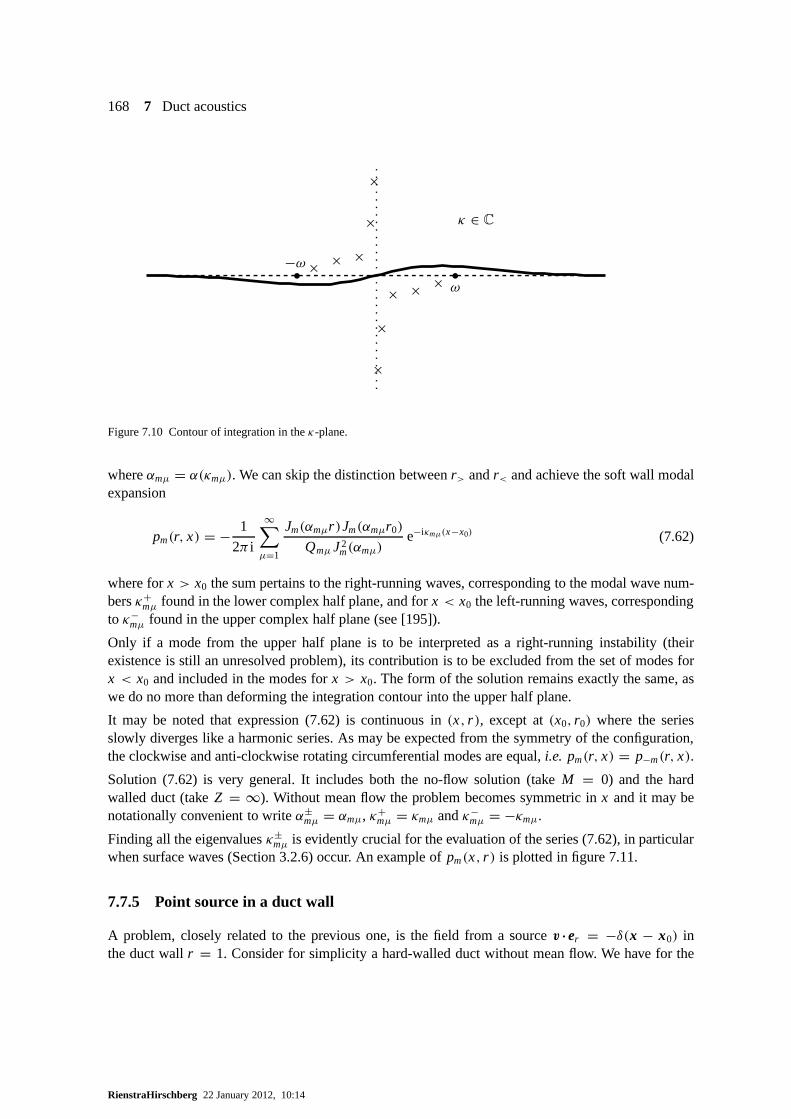
168 7 Duct acoustics
κ ∈ C
•ω
•−ω
××
×
×
×
×
×
×
×
×
Figure 7.10 Contour of integration in theκ-plane.
whereαmµ = α(κmµ). We can skip the distinction betweenr> andr< and achieve the soft wall modalexpansion
pm(r, x) = − 1
2π i
∞∑
µ=1
Jm(αmµr )Jm(αmµr0)
Qmµ J2m(αmµ)
e−iκmµ(x−x0) (7.62)
where forx > x0 the sum pertains to the right-running waves, correspondingto the modal wave num-bersκ+
mµ found in the lower complex half plane, and forx < x0 the left-running waves, correspondingto κ−
mµ found in the upper complex half plane (see [195]).
Only if a mode from the upper half plane is to be interpreted asa right-running instability (theirexistence is still an unresolved problem), its contribution is to be excluded from the set of modes forx < x0 and included in the modes forx > x0. The form of the solution remains exactly the same, aswe do no more than deforming the integration contour into theupper half plane.
It may be noted that expression (7.62) is continuous in(x, r ), except at(x0, r0) where the seriesslowly diverges like a harmonic series. As may be expected from the symmetry of the configuration,the clockwise and anti-clockwise rotating circumferential modes are equal,i.e. pm(r, x) = p−m(r, x).
Solution (7.62) is very general. It includes both the no-flowsolution (takeM = 0) and the hardwalled duct (takeZ = ∞). Without mean flow the problem becomes symmetric inx and it may benotationally convenient to writeα±
mµ = αmµ, κ+mµ = κmµ andκ−
mµ = −κmµ.
Finding all the eigenvaluesκ±mµ is evidently crucial for the evaluation of the series (7.62), in particular
when surface waves (Section 3.2.6) occur. An example ofpm(x, r ) is plotted in figure 7.11.
7.7.5 Point source in a duct wall
A problem, closely related to the previous one, is the field from a sourcev ·er = −δ(x − x0) inthe duct wallr = 1. Consider for simplicity a hard-walled duct without mean flow. We have for the
RienstraHirschberg 22 January 2012, 10:14
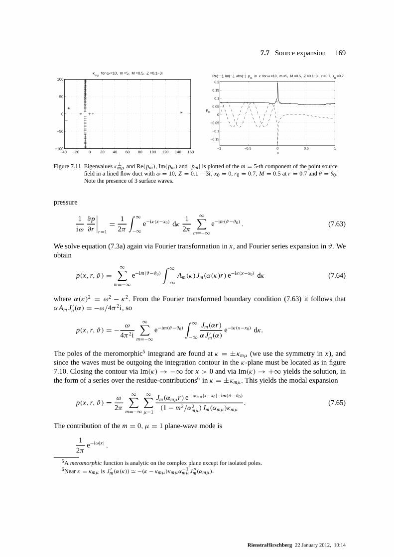
7.7 Source expansion 169
−40 −20 0 20 40 60 80 100 120 140 160−100
−50
0
50
100
κmµ for ω =10, m =5, M =0.5, Z =0.1−3i
−1 −0.5 0 0.5 1
−0.15
−0.1
−0.05
0
0.05
0.1
0.15
0.2
Re(−−), Im(−.), abs(−) pm
in x for ω =10, m =5, M =0.5, Z =0.1−3i, r =0.7, r0 =0.7
pm
x
Figure 7.11 Eigenvaluesκ±mµ and Re(pm), Im(pm) and|pm| is plotted of them = 5-th component of the point source
field in a lined flow duct withω = 10, Z = 0.1 − 3i, x0 = 0, r0 = 0.7, M = 0.5 atr = 0.7 andθ = θ0.Note the presence of 3 surface waves.
pressure
1
iω
∂p
∂r
∣∣∣∣r=1
= 1
2π
∫ ∞
−∞e−iκ(x−x0) dκ
1
2π
∞∑
m=−∞e−im(ϑ−ϑ0) . (7.63)
We solve equation (7.3a) again via Fourier transformation in x, and Fourier series expansion inϑ . Weobtain
p(x, r, ϑ) =∞∑
m=−∞e−im(ϑ−ϑ0)
∫ ∞
−∞Am(κ)Jm(α(κ)r )e−iκ(x−x0) dκ (7.64)
whereα(κ)2 = ω2 − κ2. From the Fourier transformed boundary condition (7.63) itfollows thatαAmJ ′
n(α) = −ω/4π2i , so
p(x, r, ϑ) = − ω
4π2i
∞∑
m=−∞e−im(ϑ−ϑ0)
∫ ∞
−∞
Jm(αr )
αJ ′m(α)
e−iκ(x−x0) dκ.
The poles of the meromorphic5 integrand are found atκ = ±κmµ (we use the symmetry inx), andsince the waves must be outgoing the integration contour in theκ-plane must be located as in figure7.10. Closing the contour via Im(κ) → −∞ for x > 0 and via Im(κ) → +∞ yields the solution, inthe form of a series over the residue-contributions6 in κ = ±κmµ. This yields the modal expansion
p(x, r, ϑ) = ω
2π
∞∑
m=−∞
∞∑
µ=1
Jm(αmµr )e−iκmµ|x−x0|−im(ϑ−ϑ0)
(1 − m2/α2mµ)Jm(αmµ)κmµ
. (7.65)
The contribution of them = 0, µ = 1 plane-wave mode is
1
2πe−iω|x| .
5A meromorphicfunction is analytic on the complex plane except for isolated poles.6Nearκ = κmµ is J ′
m(α(κ)) ' −(κ − κmµ)κmµα−1mµJ ′′
m(αmµ).
RienstraHirschberg 22 January 2012, 10:14
170 7 Duct acoustics
7.7.6 Vibrating duct wall
When, instead of a point, a finite part of the wall vibrates (e.g.[109]) as
r = 1 − η(x, ϑ)eiωt for − L 6 x 6 L (7.66)
then the solution may be found as follows. We write as a Fourier sum
η(x, ϑ) =∞∑
m=−∞e−imϑ ηm(x) =
∞∑
m=−∞e−imϑ
∫ ∞
−∞ηm(κ)e−iκx dκ.
Similar to above we find the solutionp(x, r, ϑ) as a formal Fourier integral, which can be rewritten,by using result (7.65) and the Convolution Theorem (C.10) (p.228), as
p(x, r, ϑ) = iω2∞∑
m=−∞
∞∑
µ=1
1
κmµ
α2mµ
α2mµ − m2
Jm(αmµr )
Jm(αmµ)e−imϑ
∫ L
−Lηm(x
′)e−iκmµ|x−x′| dx′ (7.67)
with the plane-wave contribution
iω∫ L
−Lη0(x
′)e−iω|x−x′| dx′.
A naive interpretation of this formula might suggest the contradictory result that the field, built up fromhard-wall modes with vanishingr -derivative at the wall, does not satisfy the boundary condition ofthe moving wall. This is not the case, however, because the infinite series is not uniformly converging(at least, its radial derivative). Pointwise, the value at the wall is not equal to the limit to the wall,while it is only the limit which is physically relevant.
Although in the source region no simple modes can be recognized, outside this region,i.e. for |x| > L,the remaining integral is just the Fourier transform times exponential,ηm(±κmµ)exp(−κmµ|x|), andthe solution is again just a modal sum of right- or left-running modes.
7.8 Reflection and transmission at a discontinuity in diameter
One single modal representation is only possible in segments of a duct with constant properties (di-ameter, wall impedance). When two segments of different properties are connected to each other wecan use a modal representation in each segment, but since themodes are different we have to reformu-late the expansion of the incident field into an expansion of the transmitted field in the neighbouringsegment, using conditions of continuity of pressure and velocity. This is called:mode matching. Fur-thermore, these continuity conditions cannot be satisfied with a transmission field only, and a partof the incident field is reflected. Each mode is scattered intoa modal spectrum of transmitted andreflected modes.
Consider a duct with a discontinuity in diameter atx = 0 (figure 7.12): a radiusa alongx < 0 and aradiusb alongx > 0, with (for definiteness)a > b. Because of circumferential symmetry there is noscattering into otherm-modes, so we will consider only a singlem-mode.
The fieldpin, incident fromx = −∞ and given by (see equation 7.14)
pin =∞∑
µ=1
AmµUmµ(r )e−ikmµx−imϑ , (7.68a)
RienstraHirschberg 22 January 2012, 10:14
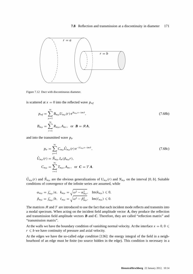
7.8 Reflection and transmission at a discontinuity in diameter 171
r = a
r = b
Figure 7.12 Duct with discontinuous diameter.
is scattered atx = 0 into the reflected wavepref
pref =∞∑
µ=1
BmµUmµ(r )eikmµx−imϑ, (7.68b)
Bmµ =∞∑
ν=1
Rmµν Amν , or B = RA,
and into the transmitted waveptr
ptr =∞∑
µ=1
CmµUmµ(r )e−i`mµx−imϑ, (7.68c)
Umµ(r ) = Nmµ Jm(βmµr ),
Cmµ =∞∑
ν=1
TmµνAmν , or C = T A.
Umµ(r ) and Nmµ are the obvious generalizations ofUmµ(r ) and Nmµ on the interval[0,b]. Suitableconditions of convergence of the infinite series are assumed, while
αmµ = j ′mµ/a, kmµ =
√ω2 − α2
mµ, Im(kmµ) 6 0,
βmµ = j ′mµ/b, `mµ =
√ω2 − β2
mµ, Im(`mµ) 6 0.
The matricesR andT are introduced to use the fact that each incident mode reflects and transmits intoa modal spectrum. When acting on the incident field amplitudevector A, they produce the reflectionand transmission field amplitude vectorsB andC. Therefore, they are called “reflection matrix” and“transmission matrix”.
At the walls we have the boundary condition of vanishing normal velocity. At the interfacex = 0,0 6
r 6 b we have continuity of pressure and axial velocity.
At the edges we have the so-callededge condition[136]: the energy integral of the field in a neigh-bourhood of an edge must be finite (no source hidden in the edge). This condition is necessary in a
RienstraHirschberg 22 January 2012, 10:14
172 7 Duct acoustics
geometry with edges because the boundary conditions lose their meaning at an edge, whereas the dif-ferential equation is not valid at the boundary. In the context of modal series expansions this conditionis related to the convergence rate of the series. Aδ-function type of a spurious edge source generates adivergent series expansion (to be interpreted as a generalized function; section C.2). Although its rôleremains in the usual engineering practice somewhat in the background, the edge condition is certainlyimportant in the present problem.
Since the problem is linear it is sufficient to determine the scattered field of a singleµ-mode. It thenfollows that the continuity of pressure at the interface
∞∑
ν=1
(Rmνµ + δνµ)Umν =∞∑
ν=1
TmνµUmν (7.69)
yields, after multiplication withUmλ(r )r , integration from 0 tob, and using orthonormality, the fol-lowing relation7 to expressTmλµ in the vectorRm·µ:
∞∑
ν=1
⟨Umλ ,Umν
⟩b(Rmνµ + δνµ) = Tmλµ, (7.70)
where
⟨f ,g
⟩b
=∫ b
0f (r )g(r )r dr.
This integral may be evaluated by using equations (D.57) and(D.58). The continuity of axial velocityat the interface
∞∑
ν=1
kmν(Rmνµ − δνµ)Umν = −∞∑
ν=1
`mνTmνµUmν (7.71)
yields, after multiplication withUmλ(r )r , integration from 0 toa of the left hand side, and from 0 tob of the right hand side, usingpx = 0 onb 6 r 6 a, the following relation expressingRmλµ in thevectorTm·µ:
kmλ(Rmλµ − δλµ) = −∞∑
ν=1
⟨Umλ ,Umν
⟩b`mνTmνµ. (7.72)
Both equations (7.70) and (7.72) are valid for anyλ andµ, so we can write in matrix notation
M(R + I ) = T ,
k (R − I ) = M>` T ,(7.73)
for identity matrix I , matrixM and its transposeM>, and diagonal matricesk and`, given by
Mλν =⟨Umλ ,Umν
⟩b, kλν = δλνkmλ, `λν = δλν`mλ.
So we have formally the solution
R = (k − M>`M)−1(k + M>`M) (7.74)
7 δi j = 1 if i = j , δi j = 0 if i 6= j .
RienstraHirschberg 22 January 2012, 10:14
7.9 Reflection at an unflanged open end 173
which can be evaluated by standard techniques for any sufficiently large truncated matrices.
A suitable choice of truncation [125, 126, 192, 247], allowing for a certain balance between the accu-racy in x < 0 and inx > 0, is to include proportionally more terms in the wider duct:a truncationof the series of (7.70) after, say,P terms and of (7.72) afterQ terms, withP/a ' Q/b. This givestruncated matricesMQ×P, M>
P×Q, kP×P, `Q×Q, so that we obtainRP×P andTQ×P.
It should be noted that if we takeP/Q very much different froma/b, wemayconverge forP,Q → ∞to another solution (7.74) than the physical one. This is notan artefact of the method: the solution isindeed not unique, because we have not yet explicitly satisfied the edge condition. The behaviour nearthe edge depends on the way we letP and Q tend to infinity, and the edge condition is satisfied iftheir ratio remains:P/Q ' a/b.
7.8.1 The iris problem
When an abrupt contraction of the duct diameter is immediately followed by an expansion to theprevious diameter (an infinitely thin orifice plate), we callthis an iris. In this case one might betempted to solve the problem directly by matching the modal expansions at either side of the irisplate. This solution will, however, either not or very slowly converge to the correct (i.e. physical)solution.
The above method of section 7.8, however, is well applicableto this problem too, if we consider theiris as a duct (albeit of zero length) connecting the two mainducts at either side of the iris. Eachtransition (from duct 1 to the iris, and from the iris to duct 2) is to be treated as above. Since thematrices of each transition are similar, the final system of matrix equations may be further simplified[192].
7.9 Reflection at an unflanged open end
The reflection at and radiation from an open pipe end of a modalsound wave depends on the variousproblem parameters like Helmholtz numberω, mode numbersm, µ and pipe wall thickness. A canon-ical problem amenable to analysis is that of a hard-walled, cylindrical, semi-infinite pipe of vanishingwall thickness. The exact solution (by means of the Wiener-Hopf technique) was first found by Levineand Schwinger (form = 0) in their celebrated paper [116]. Generalizations for higher modes may befound in [242] and with uniform [188] or jet mean flow [146, 147].
Inside the pipe we have the incident mode with reflected field,given by p(x, r, ϑ) = pm(x, r )e−imϑ
where
pm(x, r ) = Umµ(r )e−ikmµx +∞∑
µ=1
RmµνUmµ(r )eikmν x . (7.75)
Outside the pipe we have in the far field
pm(x, r ) ' Dmµ(ξ)e−iω%
ω%(ω% → ∞), (7.76)
wherex = % cosξ , r = % sinξ , and Dmµ(ξ) is called the directivity function, and|Dmµ(ξ)| is theradiation pattern.
RienstraHirschberg 22 January 2012, 10:14

174 7 Duct acoustics
The reflection matrix{Rmµν} and the directivity function are both described by complex integrals,which have to be evaluated numerically. Some important properties are:
• At resonanceω = αmµ we have total reflection in itself,Rmµµ = −1, and no reflection in any othermode,Rmµν = 0.
• Near resonanceω ∼ αmµ the modulus|Rmµν(ω)| behaves linearly from the left, and like a squareroot from the right side; the behaviour of the phase arg(Rmµν(ω)) is similar but reversed: linearlyfrom the right and like a square root from the left.
• A reciprocity relation between theµ, ν and theν, µ-coefficients:
kmνRmµν = kmµRmνµ.
• In the forward arc, 0< ξ < 12π , Dmµ(ξ) consists of lobes (maxima interlaced by zeros), while
D01(0) = 12
√2 iω2 andDmµ(0) = 0.
• In the rearward arc,12π 6 ξ < π , Dmµ(ξ) is free of zeros, and tends to zero forξ → π if m > 1and to a finite value ifm = 0.
• If kmν is real andν 6= µ, the zeros ofDmµ(ξ) are found at
ξ = arcsin(αmν/ω).
• If the mode is cut on, the main lobe is located at
ξmµ = arcsin(αmµ/ω).
• If ω → 0, the radiation pattern of the plane wavemµ = 01 becomes spherically shaped andsmall like O(ω2), while the reflection coefficient becomesR011 ' − exp(−i 2δω), whereδ =0.6127. The dimensional distanceδa is called the end correction, sincex = δa is a fictitious pointjust outside the pipe, at which the wave appears to reflect with p = 0. See also (6.95,5.44).
Based on the method presented in [188], plots ofRmµν and|Dmµ(ξ)| may be generated, as given infigures 7.13 and 7.14.
Of the reflection coefficient we have plotted modulus|Rmµν(ω)| and phaseφmµν = arg(Rmµν) as afunction ofω = 0 . . . 7., form = 0 . . . 2 andµ, ν = 1,2. Note that the resonance (cut-off) frequenciesareω = 3.8317 and 7.0156 form = 0, ω = 1.8412 and 5.3314 form = 1, andω = 3.0542 and6.7061 form = 2.
The radiation pattern is plotted, on dB-scale, of the first radial mode (µ = 1) for m = 0 andm = 1,andω = 2,4,6. For m = 0 the main lobe is atξ01 = 0, while the zeros are found forω = 4 atξ = 73.3◦, and forω = 6 atξ = 39.7◦. Form = 1 we have the main lobe atξ11 = 67.0◦,27.4◦,17.9◦
for ω = 2,4,6. The zero is found atξ = 62.7◦ for ω = 6.
Furthermore, the trend is clear that for higher frequenciesthe refraction effects become smaller, andthe sound radiates more and more like rays [29]. It is instructive to compare the wave front velocity ofa mode (the sound speed, dimensionless 1) and the axial phasevelocityvph (7.19). As the mode spiralsthrough the duct, the wave front makes an angleξmµ with the x-axis such that cos(ξmµ) = 1/vph =kmµ/ω. Indeed,
ξmµ = arccos(kmµ/ω) = arcsin(αmµ/ω)
is the angle at which the mode radiates out of the open end,i.e. the angle of the main lobe.
RienstraHirschberg 22 January 2012, 10:14
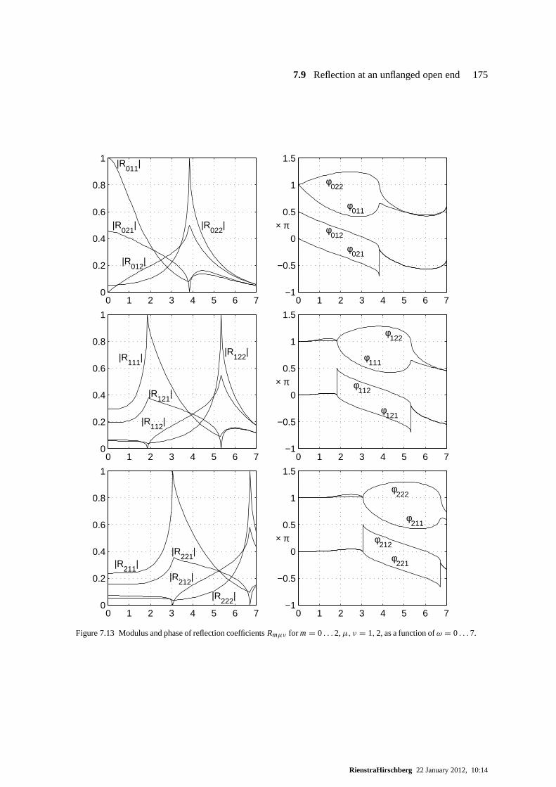
7.9 Reflection at an unflanged open end 175
0 1 2 3 4 5 6 70
0.2
0.4
0.6
0.8
1 |R011
|
|R021
|
|R012
|
|R022
|
0 1 2 3 4 5 6 7−1
−0.5
0
0.5
1
1.5
× π
φ011
φ012
φ021
φ022
0 1 2 3 4 5 6 70
0.2
0.4
0.6
0.8
1
|R111
|
|R112
|
|R121
|
|R122
|
0 1 2 3 4 5 6 7−1
−0.5
0
0.5
1
1.5
× π
φ111
φ112
φ121
φ122
0 1 2 3 4 5 6 70
0.2
0.4
0.6
0.8
1
|R211
||R
212|
|R221
|
|R222
|
0 1 2 3 4 5 6 7−1
−0.5
0
0.5
1
1.5
× π
φ211
φ212
φ221
φ222
Figure 7.13 Modulus and phase of reflection coefficientsRmµν for m = 0 . . .2,µ, ν = 1,2, as a function ofω = 0 . . .7.
RienstraHirschberg 22 January 2012, 10:14
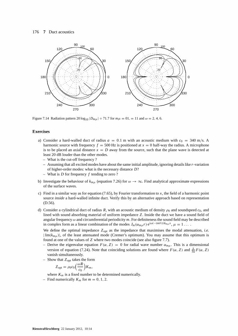
176 7 Duct acoustics
20
60
100
30
210
60
240
90
270
120
300
150
330
180 0
20
60
100
30
210
60
240
90
270
120
300
150
330
180 0
Figure 7.14 Radiation pattern 20 log10 |Dmµ| + 71.7 for mµ = 01,= 11 andω = 2, 4,6.
Exercises
a) Consider a hard-walled duct of radiusa = 0.1 m with an acoustic medium withc0 = 340 m/s. Aharmonic source with frequencyf = 500 Hz is positioned atx = 0 half-way the radius. A microphoneis to be placed an axial distancex = D away from the source, such that the plane wave is detected atleast 20 dB louder than the other modes.– What is the cut-off frequency ?– Assuming that all excited modes have about the same initialamplitude, ignoring details liker -variation
of higher-order modes: what is the necessary distanceD?– What isD for frequencyf tending to zero ?
b) Investigate the behaviour ofkmµ (equation 7.26) forω → ∞. Find analytical approximate expressionsof the surface waves.
c) Find in a similar way as for equation (7.65), by Fourier transformation tox, the field of a harmonic pointsourceinsidea hard-walled infinite duct. Verify this by an alternative approach based on representation(D.56).
d) Consider a cylindrical duct of radiusR, with an acoustic medium of densityρ0 and soundspeedc0, andlined with sound absorbing material of uniform impedanceZ. Inside the duct we have a sound field ofangular frequencyω and circumferential periodicitym. For definiteness the sound field may be describedin complex form as a linear combination of the modesJm(αmµr ) eiωt−imθ∓ikmµx, µ = 1 . . . .
We define the optimal impedanceZopt as the impedance that maximises the modal attenuation,i.e.| Im(kmµ)|, of the least attenuated mode (Cremer’s optimum). You may assume that this optimum isfound at one of the values ofZ where two modes coincide (see also figure 7.7).– Derive the eigenvalue equationF(α, Z) = 0 for radial wave numberαmµ. This is a dimensional
version of equation (7.24). Note that coinciding solutionsare found whereF(α, Z) and ∂∂α
F(α, Z)vanish simultaneously.
– Show thatZopt takes the form
Zopt = ρ0c0
(ωR
c0
)Km,
whereKm is a fixed number to be determined numerically.– Find numericallyKm for m = 0,1,2.
RienstraHirschberg 22 January 2012, 10:14
8 Approximation methods
Mathematical modelling is the art of sorting out the whole spectrum of effects that play a role in aproblem, and then making a selection by including what is relevant and excluding what is too small.This selection is what we call a “model” or “theory”. Models and theories, applicable in a certainsituation, are not “isolated islands of knowledge” provided with a logical flag, labelling it “valid” or“invalid”. A model is never unique, because it depends on thetype, quality and accuracy of answerswe are aiming for, and of course the means (time, money, numerical power, mathematical skills) thatwe have available.
Normally, when the problem is rich enough, this spectrum of effects does not simply consist of twoclasses “important” and “unimportant”, but is a smoothly distributed hierarchy varying from “essen-tial” effects via “relevant” and “rather relevant” to “unimportant” and “absolutely irrelevant” effects.As a result, in practically any model we select there will be effects that are small but not small enoughto be excluded. We can ignore this fact, and just assume that all effects that constitute our model areequally important. This is the usual approach when the problem is simple enough for analysis or abrute force numerical simulation.
There are situations, however, where it could be wise to utilise the smallness of these small but im-portant effects in such a way that we simplify the problem without reducing the quality of the model.Usually, an otherwise intractable problem becomes solvable and we gain great insight in the problem.
Perturbation methods do this in a systematic manner by usingthe sharp fillet knife of mathematics ingeneral, and asymptotic analysis in particular. From this perspective, perturbation methods are waysof modelling with other means and are therefore much more important for the understanding andanalysis of practical problems than they’re usually credited with. David Crighton [41] called “Asymp-totics - an indispensable complement to thought, computation and experiment in applied mathematicalmodelling”.
Examples are numerous: simplified geometries reducing the spatial dimension, small amplitudes al-lowing linearization, low velocities and long time scales allowing incompressible description, smallrelative viscosity allowing inviscid models, zero or infinite lengths rather than finite lengths, etc.
The question is: how can we use this gradual transition between models of different level. Of course,when a certain aspect or effect, previously absent from our model, is included in our model, the changeis abrupt and usually the corresponding equations are more complex and more difficult to solve. Thisis, however, only true if we are merely interested in exact ornumerically “exact” solutions. But anexact solution of an approximate model is not better than an approximate solution of an exact model.So there is absolutely no reason to demand the solution to be more exact than the corresponding model.If we accept approximate solutions, based on the inherent small or large modelling parameters, we dohave the possibilities to gradually increase the complexity of a model, and study small but significanteffects in the most efficient way.
The methods utilizing systematically this approach are called “perturbations methods”. Usually, adistinction is made between regular and singular perturbations. A (loose definition of a) regular per-

178 8 Approximation methods
turbation is where the solution of the approximate problem is everywhere close to the solution of theunperturbed problem.
In acoustics we have as typical examples of modelling hierarchies: wave propagation in a uniformmedium or with simple boundaries being considerably simpler than in a non-uniform medium orwith complicated boundaries. For a uniform medium and simple boundary conditions, many exactanalytical results are available. For an arbitrary non-uniform medium or complex boundary conditions,we usually have to resort to numerical methods. Analytical approximations and perturbation methodscome into play for cases in between where the problem differsonly a little from one which allows fullanalytical treatment.
We will consider here three methods relevant in acoustical problems. The first is the problem of Web-ster’s horn, an example of a regular perturbation method [127] known as method of slow variation,since the typical axial length scale is much greater than thetransverse length scale. The others are ex-amples of singular perturbation methods. The method of multiple scales (related to the WKB method)describes problems in which in the problem several length scales act in the same direction, for exam-ple a wave propagating through a slowly varying environment. The method of matched asymptoticexpansions is used to analyse problems in which several approximations, valid in spatially distinctregions, are necessary.
In order to quantify the used small effect in the model, we will always introduce a small positivedimensionless parameterε. Its physical meaning depends on the problem. It will usually stem from acharacteristic amplitude, wave number, or medium gradient.
8.1 Webster’s horn equation
Consider the following problem of low frequency sound wavespropagating in a slowly varying ductor horn [114, 197]. The typical length scale of duct variation is assumed to be much larger thana diameter, and of the same order of magnitude as the sound wave length. We introduce the ratiobetween a typical diameter and this length scale as the smallparameterε, and write for the ductsurface and wave numberk
r = R(X, θ), X = εx, k = εκ. (8.1)
A(X)`
R(X, θ)
r
θ
nn⊥
X = εx
Figure 8.1 Geometry of Webster horn.
By writing R as a function of slow variableX, rather thanx, we have made our formalassumption of slow variation explicit in aconvenient and simple way, since
∂R
∂x= ε
∂R
∂X= O(ε).
The crucial step will now be the assump-tion that the propagating sound wave isonlyaffected by the geometric variation in-duced byR. Any initial or entrance effects are absent or have disappeared. As a result the acousticfield p is a function ofX, rather thanx, and its axial gradient scales onε, as ∂
∂x p = O(ε).
RienstraHirschberg 22 January 2012, 10:14
8.1 Webster’s horn equation 179
It is convenient to introduce the following functionSand its gradients
S= r − R(X, θ), (8.2)
∇S= εSXex + Sr er + Sθr
eθ = −εRXex + er − Rθr
eθ , (8.3)
∇⊥S= Sr er + Sθr
eθ = er − Rθr
eθ . (8.4)
At the duct surfaceS = 0 the gradient∇S is a vector normal to the surface (see section A.3), whilethe transverse gradient∇⊥S, directed in the plane of a cross sectionX = const., is normal to the ductcircumferenceS(X = c, r, θ) = 0.
Inside the duct we have the reduced wave equation (Helmholtzequation)
ε2pX X + ∇2⊥ p + ε2κ2p = 0, (8.5)
at the solid wall the boundary condition of vanishing normalvelocity
∇ p ·∇S = ε2pX SX + ∇⊥ p ·∇⊥S= 0 at S= 0. (8.6)
This problem is too difficult in general, so we try to utilize in a systematic manner the small parameterε. Since the perturbation terms areO(ε2), we assume the asymptotic expansion
p(X, r, θ; ε) = p0(X, r, θ)+ ε2p1(X, r, θ)+ O(ε4).
After substitution in equation (8.5) and boundary condition (8.6), further expansion in powers ofε2
and equating like powers ofε, we obtain to leading order a Laplace equation in(r, θ)
∇2⊥ p0 = 0 with ∇⊥ p0·∇⊥S = 0 at S= 0.
An obvious solution isp0 ≡ 0. Since the solution of the Laplace equation with boundary conditionsin the normal derivative are unique up to a constant (here: a function ofX), we have
p0 = p0(X).
To obtain an equation forp0 in X we continue with theO(ε2)-equation and corresponding boundarycondition
∇2⊥ p1 + p0X X + κ2p0 = 0, ∇⊥ p1·∇⊥S= − p0X SX. (8.7)
The boundary condition can be rewritten as
∇⊥ p1·n⊥ = p0X RX
|∇⊥S| = p0X RRX√R2 + R2
θ
wheren⊥ = ∇⊥S/|∇⊥S| is the transverse unit normal vector. By integrating equation (8.7) over across sectionA of areaA(X), using Gauss’ theorem, and noting thatA =
∫ 2π0
12 R2 dθ , and that a
circumferential line element is given by d` = (R2 + R2θ )
1/2dθ , we obtain∫∫
A
∇2⊥ p1 + p0X X + κ2 p0 dσ =
∫
∂A
∇⊥ p1·n⊥ d`+ A( p0X X + κ2 p0) =
p0X
2π∫
0
RRX dθ + A( p0X X + κ2 p0) = AX p0X + A( p0X X + κ2p0) = 0.
RienstraHirschberg 22 January 2012, 10:14
180 8 Approximation methods
Finally, we have obtained for the leading order fieldp0 the Webster horn equation [12, 56, 141, 173,211, 212, 241], which is, for convenience written in the original variablesx andk, given by
1
A
d
dx
(A
d
dxp0
)+ k2 p0 = 0. (8.8)
By introducingA = D2 andφ = Dp0, the equation may be transformed into
φ′′ +(k2 − D′′
D
)φ = 0. (8.9)
This can be solved analytically for certain families of cross sectional shapesA. For example, the termD′′/D becomes a constant if
D = a emx +be−mx,
(parameterized bya, b, andm), and the equation (8.8) simplifies to
φ′′ + (k2 − m2)φ = 0
which can be solved by elementary methods. In the special casem → 0 such thata = 12(A0 + A1/m)
andb = 12(A0 − A1/m), the shape reduces to the conical hornA = (A0 + A1x)2. Forb = 0 we have
the exponential horn, and ifb = a the catenoidal horn.
The parameterm is clearly most important since it determines whether the wave is propagating (m<
k) or cut-off (m> k).
8.2 Multiple scales
Introduction
By means of the method of multiple scales we will consider problems typically of waves propagatingin a slowly varying but otherwise infinite medium (ray acoustics), or waves propagating in a slowlyvarying duct.
In both cases there is a small parameter in the problem which is the corner stone of the approximation.This small parameter is the ratio between a typical wave length and the length scale over which themedium or duct varies considerably (say, order 1).
Intuitively, it is clear that over a short distance (a few wave lengths) the wave only sees a constantmedium or geometry, and will propagate approximately as in the constant case, but over larger dis-tances it will somehow have to change its shape in accordancewith its new environment.
A technique, utilizing this difference between small scaleand large scale behaviour is the method ofmultiple scales ([153, 13]). As with most approximation methods, this method has grown out of prac-tice, and works well for certain types of problems. Typically, the multiple scale method is applicableto problems with on the one hand a certain global quantity (energy, power) which is conserved oralmost conserved and controls the amplitude, and on the other hand two rapidly interacting quantities(kinetic and potential energy) controlling the phase.
RienstraHirschberg 22 January 2012, 10:14
8.2 Multiple scales 181
An illustrative example
We will illustrate the method by considering a damped harmonic oscillator
d2y
dt2+ 2ε
dy
dt+ y = 0 (t > 0), y(0) = 0,
dy(0)
dt= 1 (8.10)
with 0< ε � 1. The exact solution is readily found to be
y(t) = sin(√
1 − ε2 t)e−εt /√
1 − ε2 (8.11)
A naive approximation for smallε and fixedt would give
y(t) = sint − εt sint + O(ε2) (8.12)
which appears to be not a good approximation for larget for the following reasons:
1) if t = O(ε−1) the second term is of equal importance as the first term and nothing is left over ofthe slow exponential decay;
2) if t = O(ε−2) the phase has an error ofO(1) giving an approximation of which even the sign maybe in error.
In the following we shall demonstrate that this type of erroroccurs also if we construct a straight-forward approximate solution directly from equation (8.10). However, knowing the character of theerror, we may then try to avoid them. Suppose we can expand
y(t; ε) = y0(t)+ εy1(t)+ ε2y2(t)+ · · · . (8.13)
Substitute in (8.10) and collect equal powers ofε:
O(ε0) : d2y0
dt2+ y0 = 0 with y0(0) = 0,
dy0(0)
dt= 1,
O(ε1) : d2y1
dt2+ y1 = −2
dy0
dtwith y1(0) = 0,
dy1(0)
dt= 0,
then
y0(t) = sint, y1(t) = −t sint, etc.
Indeed, the straightforward, Poincaré type, expansion (8.13) that is generated breaks down for larget , whenεt > O(1). As is seen from the structure of the equations foryn, the quantityyn is excited(by the “source”-terms−2dyn−1/dt) in its eigenfrequency, resulting in resonance. The algebraicallygrowing terms of the typetn sint and tn cost that are generated are called in this context:secular1
terms.
Apart from being of limited validity, the expansion revealsnothing of the real structure of the solution:a slowly decaying amplitude and a frequency slightly different from 1. For certain classes of problemsit is therefore advantageous to incorporate this structureexplicitly in the approximation.
Introduce the slow time scale
T = εt (8.14)
1From astronomical applications where these terms occurredfor the first time in this type of perturbation series: secular≈ occurring once in a century; saeculum= generation, about 100 years.
RienstraHirschberg 22 January 2012, 10:14
182 8 Approximation methods
and identify the solutiony with a suitably chosen other functionY that depends on both variablestandT :
y(t; ε) = Y(t, T; ε). (8.15)
The underlying idea is the following. There are, of course, infinitely many functionsY(t, T; ε) thatare equal toy(t, ε) along the lineT = εt in (t, T)-space. So we have now some freedom to prescribeadditional conditions. With the unwelcome appearance of secular terms in mind it is natural to thinkof conditions, chosen such that no secular terms occur when we construct an approximation.
Since the time derivatives ofy turn into partial derivatives ofY
dy
dt= ∂Y
∂t+ ε
∂Y
∂T, (8.16)
equation (8.10) becomes forY
∂2Y
∂t2+ Y + 2ε
(∂Y
∂t+ ∂2Y
∂t∂T
)+ ε2
(∂2Y
∂T2+ 2
∂Y
∂T
)= 0. (8.17)
Assume the expansion
Y(t, T; ε) = Y0(t, T)+ εY1(t, T)+ ε2Y2(t, T)+ · · · (8.18)
and substitute this into equation (8.17) to obtain to leading orders
∂2Y0
∂t2+ Y0 = 0,
∂2Y1
∂t2+ Y1 = −2
∂Y0
∂t− 2
∂2Y0
∂t∂T,
with initial conditions
Y0(0,0) = 0,∂
∂tY0(0,0) = 1,
Y1(0,0) = 0,∂
∂tY1(0,0) = − ∂
∂TY0(0,0).
The solution forY0 is easily found to be
Y0(t, T) = A0(T) sint with A0(0) = 1, (8.19)
which gives a right-hand side for theY1-equation of
−2(
A0 + ∂A0
∂T
)cost.
No secular terms occur (no resonance betweenY1 andY0) if this term vanishes:
A0 + ∂A0
∂T= 0 −→ A0 = e−T . (8.20)
Note (this is typical), that we determineY0 fully only on the level ofY1, however, without having tosolveY1 itself.
RienstraHirschberg 22 January 2012, 10:14
8.2 Multiple scales 183
The present approach is by and large the multiple scale technique in its simplest form. Variations onthis theme are sometimes necessary. For example, we have notcompletely got rid of secular terms. Ona longer time scale (t = O(ε−2)) we have inY2 again resonance because of the “source”:e−T sint ,yielding termsO(ε2t). We see that a second time scaleT2 = ε2t is necessary.
Sometimes, the occurrence of higher order time scales is really an artefact of the fast variable beingslowly varying due to external effects, like a slowly varying problem parameter. In this case the fastvariable is to be strained locally by a suitable strain function in the following way
t = 1
ε
∫ εt
ω(τ ; ε)dτ. (8.21)
(The need for the 1/ε-factor is immediately clear if we observe thatt = ε−1ωεt = ωt for a constantω = O(1).) For linear wave-type problems we may anticipate the structure of the solution and assumethe WKB hypothesis (see [13, 80])
y(t; ε) = A(T; ε)ei ε−1∫ T
0 ω(τ ;ε) dτ . (8.22)
We have
∂y
∂t=
(iωA + ε
∂A
∂T
)ei ε−1
∫ T0 ω dτ
∂2y
∂t2=
(−ω2A + 2iεω
∂A
∂T+ i ε
∂ω
∂TA + ε2∂
2A
∂T2
)ei ε−1
∫ T0 ω dτ
so that substitution in (8.10) and suppressing the exponential factor yields
(1 − ω2)A + i ε(2ω∂A
∂T+ ∂ω
∂TA + 2ωA
)+ ε2
(∂2A
∂T2+ 2
∂A
∂T
)= 0.
Note that the secular terms are now not explicitly suppressed. The necessary additional condition ishere that the solution of the present typeexists(assumption 8.22), and that each higher order correctionis no more secular than its predecessor. With some luck and ingenuity this is just sufficient to determineA andω. In general, this is indeed not completely straightforward. So much freedom may be left thatambiguities can result.
Finally, the solution is found as the following expansion
A(T ; ε) = A0(T)+ εA1(T)+ ε2A2(T)+ · · ·ω(T; ε) = ω0(T)+ ε2ω2(T)+ · · · .
(8.23)
Note thatω1 may be set to zero since the factor exp(i∫ T
0 ω1(τ )dτ) may be incorporated inA. Substi-tute and collect equal powers ofε:
O(ε0) : (1 − ω20)A0 = 0 → ω0 = 1,
O(ε1) : ∂A0
∂T+ A0 = 0 → A0 = e−T ,
O(ε2) : 2i(∂A1
∂T+ A1
)= (1 + 2ω2)e−T → ω2 = −1
2, A1 = 0.
The solution that emerges is indeed consistent with the exact solution.
RienstraHirschberg 22 January 2012, 10:14

184 8 Approximation methods
8.3 Helmholtz resonator with non-linear dissipation
An interesting application of the multiple scale techniqueis the Helmholtz resonator, derived in equa-tion (5.41). In this way we will be able to investigate the small non-linear terms that will be seen torepresent a small damping.
We start with equation (5.41)
`V
c20Sn
d2 p′in
dt2+ V2
2ρ0c40S2
n
dp′in
dt
∣∣∣∣dp′
in
dt
∣∣∣∣ + RV
ρ0c20Sn
dp′in
dt+ p′
in = p′ex. (5.41)
where we wrote for simplicity := `+ 2δ.
For a proper analysis it is most clarifying to rewrite the equation into non-dimensional variables. Forthis we need an inherent timescale and pressure. For vanishing amplitudes and negligible dissipa-tion the equation describes a harmonic oscillator, so the reciprocal of its angular frequencyω0 =(c2
0Sn/`V)1/2 is the obvious timescale of the problem. By dividing the nonlinear damping term by theacceleration term we find the pressure level 2ρ0c2
0`Sn/V at which the nonlinear damping would bejust as large as the other terms. So for a pressure that is a small fraction ε of this level we have a prob-lem with only little nonlinear damping. In addition we assume that the linear damping is small and (tomake the problem interesting) of the same order of magnitudeas the nonlinear damping. Anticipatingthe fact that we will consider (in the forced problem) the external pressure exciting near resonance,the driving amplitudep′
ex will be an order smaller thanp′in.
In order to make all this explicit we introduce a small parameter ε (selected, as we just explained, viathe external forcing amplitude), and make dimensionless
τ = ω0t, ω0 =(
c20Sn
`V
) 12
, R = ερ0c0
(`Sn
V
) 12
r,
p′in = 2ερ0c2
0`Sn
Vy, p′
ex = 2ε2ρ0c20`Sn
VF, where 0< ε � 1,
(8.24)
to obtain
d2y
dτ 2+ ε
dy
dτ
∣∣∣∣dy
dτ
∣∣∣∣ + εrdy
dτ+ y = εF. (8.25)
The initial value problem
We will start with the response to a stepwise change of external pressure, so we assumeF = 0, andprescribe ay = 1 at t = 0. This yields the problem
d2y
dτ 2+ ε
dy
dτ
∣∣∣∣dy
dτ
∣∣∣∣ + εrdy
dτ+ y = 0, with y(0) = 1,
dy(0)
dτ= 0. (8.26)
By comparing the accelerationy′′ with the dampingε(y′|y′| + r y′) it may be inferred that on atimescaleετ the influence of the damping isO(1). So we conjecture a slow timescaleετ , and split upthe time dependence in two by introducing the slow timescaleT and the dependent variableY
T = ετ, y(τ ; ε) = Y(t, T; ε), dy
dτ= ∂Y
∂τ+ ε
∂Y
∂T,
RienstraHirschberg 22 January 2012, 10:14
8.3 Helmholtz resonator with non-linear dissipation 185
and obtain for equation (8.26)
∂2Y
∂τ 2+ Y + ε
(2∂2Y
∂τ∂T+ ∂Y
∂τ
∣∣∣∣∂Y
∂τ
∣∣∣∣ + r∂Y
∂τ
)+ O(ε2) = 0
Y(0,0; ε) = 1,( ∂∂τ
+ ε∂
∂T
)Y(0,0; ε) = 0.
(8.27)
The error ofO(ε2) results from the approximation∂∂τ
Y + ε ∂∂T Y ' ∂
∂τY, and is of course only valid
outside a small neighbourhood of the points where∂∂τ
Y = 0. We assume the regular expansion
Y(t, T; ε) = Y0(t, T)+ εY1(t, T)+ O(ε2)
and find for the leading order
∂2Y0
∂τ 2+ Y0 = 0, with Y0(0,0) = 1,
∂
∂τY0(0,0) = 0 (8.28)
with solution
Y0 = A0(T) cos(τ −20(T)), where A0(0) = 1, 20(0) = 0.
For the first order we have the equation
∂2Y1
∂τ 2+ Y1 = −2
∂2Y0
∂τ∂T− ∂Y0
∂τ
∣∣∣∣∂Y0
∂τ
∣∣∣∣ − r∂Y0
∂τ= 2
dA0
dTsin(τ −20)
− 2A0d20
dTcos(τ −20)+ A2
0 sin(τ −20)| sin(τ −20)| + r A0 sin(τ −20) (8.29)
with corresponding initial conditions (they are unimportant for the leading order result). The secularterms are suppressed if the first harmonics (cos and sin) of the right-hand side cancel. For this we usethe Fourier series expansion (section C.3, eq. C.45e)
sinτ | sinτ | = − 8
π
∞∑
n=0
sin(2n + 1)τ
(2n − 1)(2n + 1)(2n + 3)(8.30)
and we obtain the equations
2dA0
dT+ 8
3πA2
0 + r A0 = 0 andd20
dT= 0 (8.31)
with solution20 = 0 and
A0(T) =12r
(4
3π + 12r
)e
12rT − 4
3π
(8.32)
With little linear dissipation (r small) this reduces to an algebraic decay,viz. A0(T) = (1 + 43π T)−1,
and with little nonlinear dissipation (r large) to the exponential decayA0(T) = e− 12rT . All together
we have
pin ' 2ερ0c20`Sn
V
12r cosτ
(4
3π + 12r
)e
12r ετ − 4
3π
, with τ =(
c20Sn
`V
) 12
t. (8.33)
Comparison with a numerically obtained “exact” solution shows that this approximation happens tobe quite good.
RienstraHirschberg 22 January 2012, 10:14
186 8 Approximation methods
The response to harmonic forcing
Suppose we excite the Helmholtz resonator harmonically by an external forcingp′ex = C cos(ωt) of
frequencyω. In the scaled variablesτ andF this becomes
εF = εF0 cos(�τ), with ω = �ω0.
So we have the forced oscillator
d2y
dτ 2+ ε
dy
dτ
∣∣∣∣dy
dτ
∣∣∣∣ + εrdy
dτ+ y = εF0 cos(�τ) (8.34)
where we don’t care about initial conditions, because we areonly interested in the stationary state.
When we stay away from resonance conditions, in other words when 1−�2 is not small, the solutionis relatively simple. The internal pressure follows the external excitation both in amplitude and intime dependence. The nonlinear terms hardly play a role, because the driving amplitude is small. Soto leading order inε we have the solution
y(τ ) = εF0(1 −�2) cos�τ + εr� sin�τ
(1 −�2)2 + ε2r 2�2= Acos(�τ − θ),
A = εF0√(1 −�2)2 + ε2r 2�2
, tanθ = εr�
1 −�2.
(8.35)
We see that near resonance this solution is not valid anymore. When 1− �2 = O(ε), amplitudeArises to levels ofO(1), and the assumption that the nonlinear damping is negligible is not correct. Atthe same time, it should be noticed that this corresponds with the most important situations (with themost achieved damping). So it is worthwhile to analyse this problem in more detail. As the physics ofthe problem essentially change when�2 = 1 + O(ε), we assume
� = 1 + ε1. (8.36)
To facilitate the analysis we remove theε-dependence from the driving force, so we make again aslight shift in the time coordinate and introduce
τ = �τ (8.37)
to obtain
�2d2y
dτ 2+ ε�2 dy
dτ
∣∣∣∣dy
dτ
∣∣∣∣ + ε�rdy
dτ+ y = εF0 cos(τ ) (8.38)
To leading order this becomes
(1 + 2ε1)d2y
dτ 2+ ε
dy
dτ
∣∣∣∣dy
dτ
∣∣∣∣ + εrdy
dτ+ y = εF0 cos(τ ) (8.39)
When we substitute the assumed expansiony(τ ; ε) = y0(τ ) + εy1(τ )+ . . . , and collect like powersof ε, we find fory0
d2y0
dτ 2+ y0 = 0 (8.40)
RienstraHirschberg 22 January 2012, 10:14

8.3 Helmholtz resonator with non-linear dissipation 187
with general solution
y0(τ ) = A0 cos(τ − θ0). (8.41)
Although y0 is the result of driving forceF , we don’t have any information yet so we can’t determinethe integration constantsA0 andθ0 at this level. Therefore we continue with the next ordery1.
d2y1
dτ 2+ y1 = F0 cos(τ )− 21
d2y0
dτ 2− dy0
dτ
∣∣∣∣dy0
dτ
∣∣∣∣ − rdy0
dτ
= F0 cos(τ )+ 21A0 cos(τ − θ0)+ A20 sin(τ − θ0)
∣∣sin(τ − θ0)∣∣ + r A0 sin(τ − θ0). (8.42)
From the argument that we are only interested in the stationary state it follows that no resonant ex-citation is allowed in the right-hand-side of the equation for y1. This is effectively very similar tothe condition of absent secular terms of the previous initial value problem. So we can use the sametechniques to suppress the cos- and sin-terms, and use equation (8.30) to obtain
(4
3π A20 + 1
2r A0)
sin(θ0)−1A0 cos(θ0) = 12 F0(
43π A2
0 + 12r A0
)cos(θ0)+1A0 sin(θ0) = 0
(8.43)
with solution
[(4
3π A0 + 12r
)2 +12]A2
0 = 14 F2
0 , tanθ0 = −1−1(
43π A0 + 1
2r)
(8.44)
This equation has several solutions, and it is not immediately clear which is the correct one. To solveA0 = A0(1) is difficult, but it is easy to write1 = 1(A0):
12 = F20
4A20
−( 4
3πA0 + 1
2r)2.
Since12 > 0 we see immediately that solutions exists only for a finite interval in A0, while1 → ∞only whenA0 → 0. In particular, we have
A0 = ± F0
21+ O(1−2), |1| → ∞
which is in exact agreement with the asymptotic behaviour for � = 1 + ε1, 1 large, of (8.35). Infact, by tracing the solution parametrically as a function of 1, we can see which solution is the correctone, or at least which solution connects to the non-resonantsolutions. See figure 8.2 for an example.
−5 −4 −3 −2 −1 0 1 2 3 4 5−2
−1.5
−1
−0.5
0
0.5
1
A0
1
Figure 8.2SolutionsA0 as a function of1, for r0 = 1 andF0 = 1. See eq. (8.44)
RienstraHirschberg 22 January 2012, 10:14

188 8 Approximation methods
8.4 Slowly varying ducts
Consider a hard-walled circular cylindrical duct with a slowly varying diameter (c.f. [193, 191, 200,154, 34, 196, 164],), described in polar coordinates(x, r, θ) as
r = a(εx) (8.45)
with ε a dimensionless small parameter. In this duct we have an acoustic medium with constant mean
X = εxθ
r = a(X)
Figure 8.3Sketch of geometry of slowly varying circular duct.
pressure and a slowly varying sound speedc0 = c0(εx) (for simplicity no variation inr and θ isassumed). Sound waves of circular frequencyω are described by a variant of the Helmholtz equation
∇·( 1
k2∇ p
)+ p = 0 (8.46)
wherek = k(εx) = ω/c0(εx), with boundary condition a vanishing normal velocity component atthe wall, so
n·∇ p = 0 atr = a(εx). (8.47)
Since (section A.3)
n ∝ ∇(r − a(εx)
)= er − εa′(εx)ex,
(wherea′(z) = da(z)/dz) this is
∂p
∂r− εa′(εx)
∂p
∂x= 0 atr = a(εx). (8.48)
We know that for constanta and constantk the general solution can be built up from modes of thefollowing type (chapter 7)
p = AJm(αmµr )e−imθ−ikmµx, (8.49)
αmµ = j ′mµ/a,
k2mµ = k2 − α2
mµ, Re(kmµ) > 0, Im(kmµ) 6 0,
and we assume for the present problem, following the previous section, that there are solutions closeto these modes. We introduce the slow variable
X = εx
RienstraHirschberg 22 January 2012, 10:14
8.4 Slowly varying ducts 189
so thatk = k(X), and we seek a solution of slowly varying modal type:
p = A(X, r ; ε)e−imθ e−i ε−1∫ X
0 γ (ξ ;ε) dξ (8.50)
Since
∇·( 1
k2∇ p
)= ∂
∂x
( 1
k2
∂p
∂x
)+ 1
k2
(∂2 p
∂r 2+ 1
r
∂p
∂r+ 1
r 2
∂2 p
∂θ2
)
∂p
∂x=
(−iγ A + ε
∂A
∂X
)exp
(· · ·
)
∂2 p
∂x2=
(−γ 2A − 2iεγ
∂A
∂X− i ε
∂γ
∂XA + ε2 ∂
2A
∂X2
)exp
(· · ·
)
we have for (8.46) after multiplication withk2:
[−γ 2A − 2iεγ
∂A
∂X− i ε
∂γ
∂XA + ε2 ∂
2A
∂X2− 2ε
1
k
∂k
∂X
(−iγ A + ε
∂A
∂x
)
+∂2A
∂r 2+ 1
r
∂A
∂r− m2
r 2A + k2A
]exp
(· · ·
)= 0.
After suppressing the exponential factor, this is up to order O(ε)
L(A) = i εk2
A
∂
∂X
(γ A2
k2
),
∂A
∂r+ i ε
∂a
∂Xγ A = 0 atr = a(X),
(8.51)
where we introduced for short the Bessel-type operator (seeAppendix D)
L(A) = ∂2A
∂r 2+ 1
r
∂A
∂r+
(k2 − γ 2 − m2
r 2
)A
and rewrote the right-hand side in a form convenient later. Expand
A(X, r ; ε) = A0(X, r )+ εA1(X, r )+ O(ε2)
γ (X; ε) = γ0(X)+ O(ε2)
substitute in (8.51), and collect like powers ofε.
O(1) : L(A0) = 0 (8.52)
∂A0
∂r= 0 atr = a(X),
O(ε) : L(A1) = ik2
A0
∂
∂X
(γ0A20
k2
)(8.53)
∂A1
∂r= −i
∂a
∂Xγ0A0 at r = a(X).
RienstraHirschberg 22 January 2012, 10:14

190 8 Approximation methods
Since variableX plays no other rôle in (8.52) than that of a parameter, we havefor A0 the “almost-mode”
A0(X, r ) = P0(X)Jm(α(X)r ),
α(X) = j ′mµ/a(X), (8.54)
γ 20 (X) = k2(X)− α2(X), Re(γ0) > 0, Im(γ0) 6 0,
The amplitudeP0 is still undetermined, and follows from a solvability condition for A1. As before,amplitudeP0 is determined at the level ofA1, without A1 necessarily being known.
Multiply left- and right-hand side of (8.53) withr A0/k2 and integrate tor from 0 to a(X). For theleft-hand side we utilize the self-adjointness ofL.
∫ a
0
r A0
k2L(A1)dr = 1
k2
∫ a
0r A0L(A1)− r A1L(A0)dr = 1
k2
[r A0
∂A1
∂r− r A1
∂A0
∂r
]a
0
= −iγ0a
k2
∂a
∂XA2
0.
For the right-hand side we apply the Leibniz integral rule
i∫ a
0
∂
∂X
(γ0A20
k2
)r dr = i
d
dX
∫ a
0
r γ0A20
k2dr − i
γ0a
k2
∂a
∂XA2
0.
As a result∫ a
0
r γ0A20
k2dr =
[γ0
2k2P2
0
(r 2 − m2
α2
)Jm(αr )2
]a
0
= γ0P20
2k2a2
(1 − m2
j ′mµ
2
)Jm( j ′
mµ)2 = constant
or:
P0(X) = const.k(X)
a(X)√γ0(X)
= const.k(X)α(X)√γ0(X)
(8.55)
It is not accidental that the above integral∫ a
0 (r γ0A20/k2)dr is constant. The transmitted power ofp is
to leading order
P =∫ 2π
0
∫ a
0
12 Re(pu∗)r dr dθ = π
ωρ0
∫ a
0Im
(p ∂∂x p∗
)r dr
= π
ωρ0Re(γ0)e2ε−1
∫ X0 Im(γ0) dξ
∫ a
0|A0|2r dr. (8.56)
This is for propagating modes (γ0 real) constant:
P = π
ωρ0γ0|P0|2 1
2a2(1 − m2
j ′mµ
2
)Jm( j ′
mµ)2 = const.
γ0
ρ0
k2
a2γ0a2 = const.
1
ρ0c20
= constant
sinceρ0c20 is, apart from a factor, equal to the constant mean pressure.
RienstraHirschberg 22 January 2012, 10:14
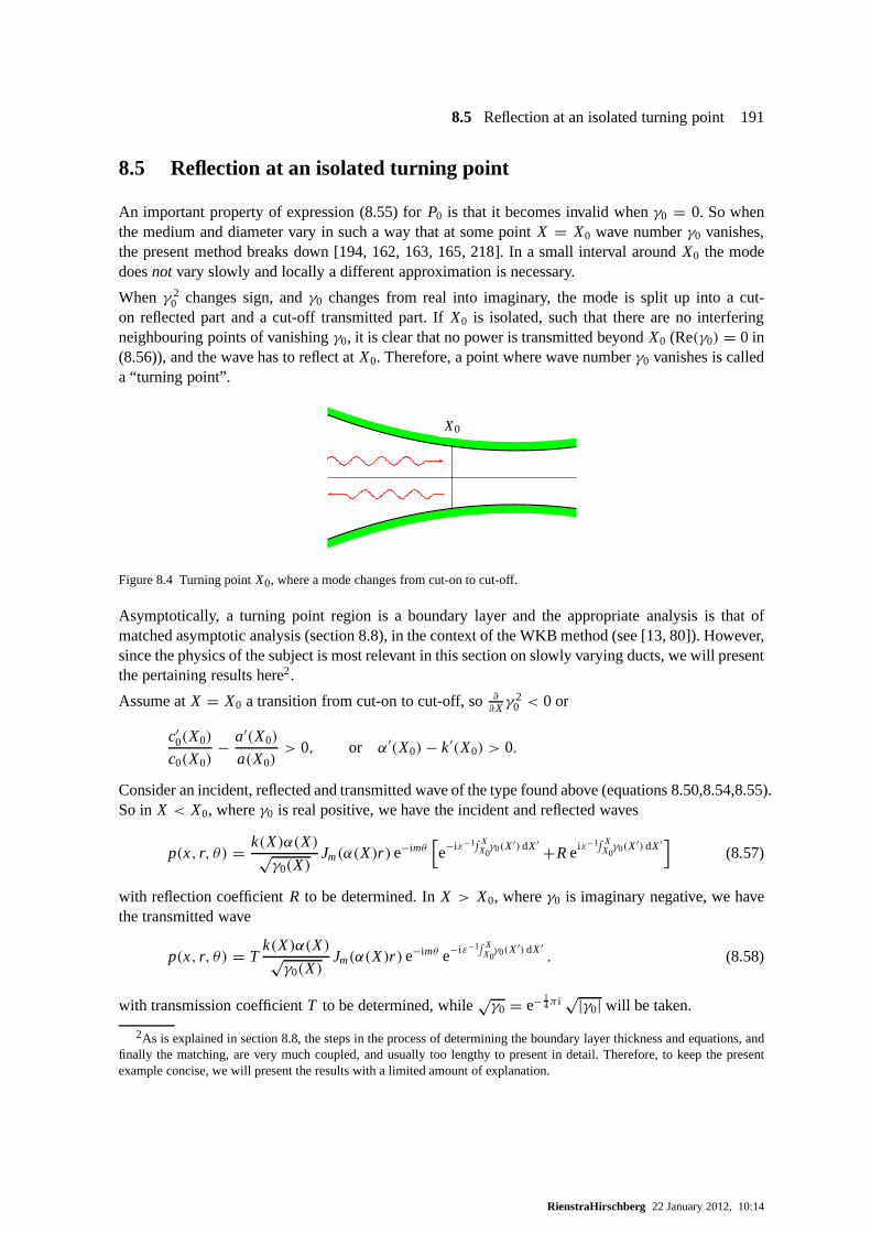
8.5 Reflection at an isolated turning point 191
8.5 Reflection at an isolated turning point
An important property of expression (8.55) forP0 is that it becomes invalid whenγ0 = 0. So whenthe medium and diameter vary in such a way that at some pointX = X0 wave numberγ0 vanishes,the present method breaks down [194, 162, 163, 165, 218]. In asmall interval aroundX0 the modedoesnot vary slowly and locally a different approximation is necessary.
When γ 20 changes sign, andγ0 changes from real into imaginary, the mode is split up into a cut-
on reflected part and a cut-off transmitted part. IfX0 is isolated, such that there are no interferingneighbouring points of vanishingγ0, it is clear that no power is transmitted beyondX0 (Re(γ0) = 0 in(8.56)), and the wave has to reflect atX0. Therefore, a point where wave numberγ0 vanishes is calleda “turning point”.
X0
Figure 8.4 Turning pointX0, where a mode changes from cut-on to cut-off.
Asymptotically, a turning point region is a boundary layer and the appropriate analysis is that ofmatched asymptotic analysis (section 8.8), in the context of the WKB method (see [13, 80]). However,since the physics of the subject is most relevant in this section on slowly varying ducts, we will presentthe pertaining results here2.
Assume atX = X0 a transition from cut-on to cut-off, so∂∂Xγ
20 < 0 or
c′0(X0)
c0(X0)− a′(X0)
a(X0)> 0, or α′(X0)− k′(X0) > 0.
Consider an incident, reflected and transmitted wave of the type found above (equations 8.50,8.54,8.55).So in X < X0, whereγ0 is real positive, we have the incident and reflected waves
p(x, r, θ) = k(X)α(X)√γ0(X)
Jm(α(X)r )e−imθ[e−i ε−1
∫ XX0γ0(X′) dX′
+Rei ε−1∫ X
X0γ0(X′) dX′]
(8.57)
with reflection coefficientR to be determined. InX > X0, whereγ0 is imaginary negative, we havethe transmitted wave
p(x, r, θ) = Tk(X)α(X)√γ0(X)
Jm(α(X)r )e−imθ e−i ε−1∫ X
X0γ0(X′) dX′
. (8.58)
with transmission coefficientT to be determined, while√γ0 = e− 1
4π i √|γ0| will be taken.
2As is explained in section 8.8, the steps in the process of determining the boundary layer thickness and equations, andfinally the matching, are very much coupled, and usually too lengthy to present in detail. Therefore, to keep the presentexample concise, we will present the results with a limited amount of explanation.
RienstraHirschberg 22 January 2012, 10:14

192 8 Approximation methods
This set of approximate solutions of equation (8.46), validoutside the turning point region, constitutethe outer solution. Inside the turning point region this approximation breaks down. The approximationis invalid here, because neglected terms of equation (8.46)are now dominant, and another approxi-mate equation is to be used. This will give us the inner or boundary layer solution. To determine theunknown constants (here:R andT), inner and outer solution are asymptotically matched.
For the matching it is necessary to determine the asymptoticbehaviour of the outer solution in thelimit X → X0, and the boundary layer thickness (i.e. the appropriate local coordinate).
From the limiting behaviour of the outer solution in the turning point region (see below), we canestimate the order of magnitude of the solution. From a balance of terms in the differential equation(8.46) it transpires that the turning point boundary layer is of thicknessX − X0 = O(ε2/3), leading toa boundary layer variableξ given by
X = X0 + ε2/3ξ.
Since forε → 0
γ 20 (X) = γ 2
0 (X0 + ε2/3ξ) = −2ε2/3k0(α′0 − k′
0)ξ + O(ε4/3ξ2),
wherek0 = k(X0), k′0 = k′(X0), etc., we have
1
ε
∫ X
X0
γ0(X′)dX′ =
{−2
3|ξ |3/2 = −ζ, if ξ < 0
−i 23 ξ
3/2 = −i ζ, if ξ > 0
where we introduced
ξ = {2k0(α′0 − k′
0)}1/3ξ and ζ = 23|ξ |
3/2.
The limiting behaviour forX ↑ X0 is now given by
p ' k0 α0
{2εk0(α′0 − k′
0)}1/6 |ξ |1/4Jm(α0r )e−imθ
(eiζ +Re−iζ
), (8.59)
while it is for X ↓ X0 given by
p ' Te
14π i k0 α0
{2εk0(α′0 − k′
0)}1/6 ξ1/4Jm(α0r )e−imθ e−ζ . (8.60)
Since the boundary layer is relatively thin, also compared to the radial coordinate, the behaviour of theincident mode remains rather unaffected in radial direction, and we can assume in the turning pointregion
p(x, r, θ) = Jm(α(X)r )ψ(ξ)e−imθ .
From the properties of the Bessel equation (D.1), we have
∂2p
∂r 2+ 1
r
∂p
∂r+ 1
r 2
∂2p
∂θ2+ k2 p = γ 2
0 p = O(ε2/3)p.
Hence, equation (8.46) yields
k2∇·( 1
k2∇ p
)+k2p ' ε2/3∂
2 p
∂ξ2+γ 2
0 p = ε2/3Jm(α(X)r )e−imθ{∂2ψ
∂ξ2−2k0(α
′0−k′
0)ξψ}
= 0
RienstraHirschberg 22 January 2012, 10:14
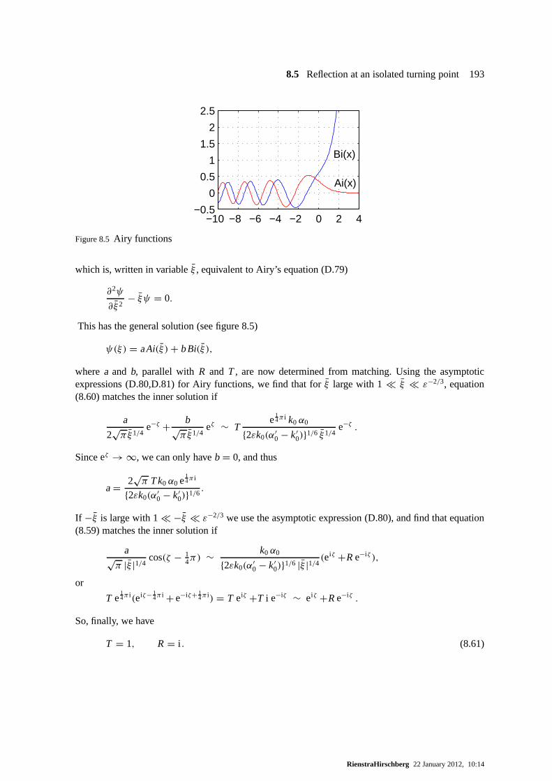
8.5 Reflection at an isolated turning point 193
−10 −8 −6 −4 −2 0 2 4−0.5
0
0.5
1
1.5
2
2.5
Ai(x)
Bi(x)
Figure 8.5Airy functions
which is, written in variableξ , equivalent to Airy’s equation (D.79)
∂2ψ
∂ξ2− ξψ = 0.
This has the general solution (see figure 8.5)
ψ(ξ) = aAi(ξ )+ bBi(ξ ),
wherea and b, parallel with R and T , are now determined from matching. Using the asymptoticexpressions (D.80,D.81) for Airy functions, we find that forξ large with 1� ξ � ε−2/3, equation(8.60) matches the inner solution if
a
2√πξ1/4
e−ζ + b√πξ1/4
eζ ∼ Te
14π i k0 α0
{2εk0(α′0 − k′
0)}1/6 ξ1/4e−ζ .
Sinceeζ → ∞, we can only haveb = 0, and thus
a = 2√π T k0 α0 e
14π i
{2εk0(α′0 − k′
0)}1/6.
If −ξ is large with 1� −ξ � ε−2/3 we use the asymptotic expression (D.80), and find that equation(8.59) matches the inner solution if
a√π |ξ |1/4
cos(ζ − 14π) ∼ k0 α0
{2εk0(α′0 − k′
0)}1/6 |ξ |1/4(ei ζ +Re−i ζ ),
or
T e14π i(eiζ− 1
4π i + e−iζ+ 14π i) = T eiζ +T i e−iζ ∼ ei ζ +Re−i ζ .
So, finally, we have
T = 1, R = i . (8.61)
RienstraHirschberg 22 January 2012, 10:14

194 8 Approximation methods
8.6 Ray acoustics in temperature gradient
When a sound wave propagates in free space through a medium that varies on a much larger scalethan the typical wave length (typically: temperature gradients, or wind with shear), the same ideas ofmultiple scales may be applied. In contrast to the duct, where the wave is confined by the duct walls,the waves may now freely refract and follow curved paths. These paths are called rays. This meansthat rays are not localized “beams” of sound, but only the tangents of the intensity vectors of a soundfield.
Consider an infinite 3D medium with varying temperature but otherwise with a constant mean pres-sure, so that we have again equation (8.46), but nowc varying more generally as a function ofx
∇·(c2
0∇ p)
+ ω2p = 0, c0 = c0(εx) (8.62)
for a time harmonic sound fieldp ∝ eiωt . The typical lengthscaleL of sound speed variations, es-timated fromL−1 ∼ ‖∇c0‖/c0, is assumed much larger than the typical wave lengthλ ∼ c0/ω. Inorder to quantify this, we writec0 = c0(εx) where the small parameterε is given byε = λ/L. In thefollowing, we will see that this introduction ofε is a convenient way of keeping the large and smallterms apart.3
Assuming the field to be locally plane we try an approximate solution having the form of a plane wavebut with slowly varying (real) amplitudeA = A(X; ε) and phaseτ = τ(X)
p(x) = Ae−iτ/ε (8.63)
whereX = εx the slow variable. The surfacesτ(X) = εωt describe the propagating wave front. Notethat the vector field∇τ is normal to the surfacesτ = constant (section A.3). Define the operator
∇ =( ∂
∂X,∂
∂Y,∂
∂Z
)
so that∇ = ε∇. Define the local wave vector
k = ∇τ, (8.64)
inspired by the fact that if we approximate locallyτ(X) = τ0 + ∇τ ·X + . . . (with τ0 an unimpor-tant constant), the wave becomes a plane wave' A0 eiωt−ik·x with frequencyω and wave vectork.Substitute (8.63) in (8.62):
∇ p =(ε∇ A − i Ak
)e−iτ/ε, (8.65a)
∇2 p =(ε2∇2
A − 2iε∇ A·k − i εA∇ ·k − A|k|2)
e−iτ/ε, (8.65b)
to obtain
(ω2 − c20|k|2)A − i εA−1∇ ·(c2
0 A2k)+ ε2∇ ·(c2
0∇ A)
= 0. (8.66)
3It should be noted that our point of view here is to think of theproblem as a wave in a slowly varying medium,i.e. toconsiderL “large”. Another, equally valid point of view is to think of amedium with a high frequency wave,i.e. to scalethe problem onL and to consider the wave length “short” or the frequency “high”.
RienstraHirschberg 22 January 2012, 10:14
8.6 Ray acoustics in temperature gradient 195
Expand
A(X; ε) = A0(X)+ εA1(X)+ O(ε2)
and collect like powers in (8.66). We find to leading order
c20|k|2 − ω2 = 0 (8.67)
∇ ·(c20 A2
0k)
= 0. (8.68)
Equation (8.67) is theeikonal equation, which determines the wave fronts and the ray paths. Equation(8.68) is called thetransport equationand describes theconservation of wave action, which is hereequivalent toconservation of energy[120, 245]. It relates the amplitude variation to divergingorconverging rays.
The eikonal equation is a nonlinear first order partial differential equation, of hyperbolic type, whichcan always be reduced to an ordinary differential equation along characteristics [35]. This is summa-rized by the following theorem ([245, p.65]).
Theorem 8.1 (General solution of 1st order PDE)The solution of the first-order partial differential equation
H (k, τ, x) = 0, k = ∇τ,
with consistent boundary conditions on a surface S, is givenby the system of ordinary differentialequations4
dχ
dλ= ∇k H,
dτ
dλ= k·∇k H,
dkdλ
= −k∂H
∂τ− ∇x H,
where the curvex = χ(λ), with parameterλ, is called a characteristic.
A characteristic forms a path along which the information ofthe boundary values on S is transferred tothe point of observation. In general the characteristic depends on the solution, and both characteristicand solution are to be determined together. If more than one point of a characteristic is part of S, theboundary conditions are not independent, and in general inconsistent. If more than one characteristicpasses through a point, the solution is not unique.
By starting from other, equivalent, equations H(k, τ, x) = 0, we obtain the same solution but withother parametrizations.
Sometimes a preferable parametrization is the so-called natural parametrization, withλ equal to thearclength and‖ d
dλχ‖ = 1.
The characteristics are here identical to the rays. By rewriting equation (8.67) as12ε(c20|k|2−ω2)/ω =
0 and using theorem (8.1) (p.195), the characteristic variable is just the timet (but not the arclength),and we have the expected
τ(X(t)) = εωt
4∇k H denotes the gradient ink: ( ∂H∂ki); similar for∇x H .
RienstraHirschberg 22 January 2012, 10:14
196 8 Approximation methods
along a rayX = X(t) given by
dXdt
= εc0k|k| . (8.69)
dkdt
= −ε ωc0
∇c0. (8.70)
Equations (8.69) and (8.70) are called: “ray-tracing equations”.
Once we know the rays, the transport equation (8.68) can be solved as follows. Consider a small areaS1 of the surfaceτ = C1, and connect the points ofS1 via the rays (following the vector fieldk) withthe corresponding areaS2 on the surfaceτ = C2. Then the volume of rays connectingS1 and S2 iscalled a ray-tube. Sincek is just parallel to the tube’s surface, except forS1 and S2 where it is justω/c0 and perpendicular to it, we have (with Gauss’ theorem)
∫
tube∇ ·(c2
0 A20k
)dX = 0 =
∫
S2
c0A20 ds −
∫
S1
c0A20 ds.
If we associate to a rayX(t) a ray-tube with cross sectionS = S(X), the amplitude varies accordingto the relation
A20(X)c0(X)S(X) = constant along a ray tube. (8.71)
From equation (8.70) it can be inferred that a ray (with direction k) bends away from regions withhigher sound speed. This explains why sound is carried far along a cold surface like water or snow, andnot at all along for example hot sand. When the surface is coldthere is a positive soundspeed gradientwhich causes the sound waves to bend downwards to the surface. In combination with reflection at thesurface the sound is trapped and tunnels through the layer adjacent to the surface. When the surfaceis hot there is a negative soundspeed gradient which causes the sound to bend upwards and so todisappear into free space.
We can make this more explicit for a sound speed that varies linearly in space. We have then theremarkable result of exact solutions of rays following plane circles. To show this in detail, it is neces-sary that we obtain a parametrization that corresponds withan arclength (in the slow coordinateX).Therefore, we recast the eikonal equation in the form
H (X, τ, k) = 1
2
(|k| − ω2
c20|k|
)(8.72)
and obtain from theorem (8.1)
dXds
= ∇k H = 1
2
k|k| + 1
2
ω2
c20|k|3
k = k|k| = t
dτ
ds= k·∇k H = k·k
|k| = |k|
dkds
= −k∂H
∂τ− ∇X H = 0 − ω2
c30|k|
∇c0 = −|k|c0
∇c0
The ray is given by the curveX = X(s) and launched atX(0) = εx(0) in the directionk(0) withinitial phaseτ(0). Since we have applied the so-called natural parametrization, with s the arclength,dds X = t is the unit tangent vector andd
2
ds2 X the curvature vector:
κ = d2Xds2
= 1
ω
d
ds
(c0k
)= 1
ω
[k|k|(∇c0·k)− |k|∇c0
](8.73)
RienstraHirschberg 22 January 2012, 10:14

8.6 Ray acoustics in temperature gradient 197
The curvature, or reciprocal radius, is then
|κ| = 1
ω
[|k|2|∇c0|2 − (∇c0·k)2
]1/2(8.74)
Now we use the fact thatc0 varies linearly in (say) directionn:
c0 = q + α(X ·n), ∇c0 = αn. (8.75)
Decompose vectork in a component inn direction and one orthogonal to it
k = k0n + k1b, with n·b = 0, |b| = 1. (8.76)
Of course,k0 = (k·n) andk1 = (k·b). It follows from
dkds
= −|k|c0
∇c0 = −|k|c0αn (8.77)
that k only varies inn-direction, whilek1b is constant, determined by the initial wave vectork(0).Since alson is fixed, it is onlyk0 = k0(s) that varies withs. So we go on with the curvature
κ = 1
ω|k|[k(∇c0·k)− |k|2∇c0
]= 1
ω|k|[(k0n + k1b)αk0 − (k2
0 + k21)αn
]
= 1
ω|k|[αk2
0n + αk0k1b − αk20n − αk2
1n]
= αk1
ω|k|(k0b − k1n) = αk1
ωc
(8.78)
where vector
c = k0b − k1n|k| (8.79)
is the unit curvature vector (or principal normal unit vector) of curveX(s). Sincen andb are constant,c, and thereforeX, is in one plane. More precisely formulated: the normal vector of the plane ofX(the so-called osculating plane ofX) is
t×c = n×b
or the unit binormal vector ofX. Sincen andb are constant, the torsion ofX
d
ds(t×c) = 0
is zero, andX is a plane curve. Furthermore, since the curvature
|κ| =∣∣∣∣αk1
ω
∣∣∣∣
is constant, the curve is a circle. The radius (inx coordinates) isR = |ω/αk1ε|, and depends on theinitial conditionk1. The center of the circle is found atx = x(0)+ Rc. See [122].
RienstraHirschberg 22 January 2012, 10:14

198 8 Approximation methods
8.7 Refraction in shear flow
The propagation of sound waves in the atmosphere is greatly affected by wind. For example, thecommunication between two people, one downstream and one upstream, is not symmetric. The oneupstream is easier to understand for the one downstream thanthe other way around. This isnotbecausethe wind “carries the waves faster”, but it is due to refraction by the wind gradient (the atmosphericboundary layer). This is seen as follows ([120]).
U (z)
Figure 8.6 Refraction in shear flow.
Consider the acoustic wave equations (2.51a-2.51d) for sound in an arbitrary mean flow. We assumethe sound field to be time harmonic with a frequency high enough to adopt a ray approximation. Thesmall parameter is now againε ∼ c0/ωL, with L a typical length scale for variations in the mean flowvelocity v0. Similar to the foregoing chapter we introduce the compressed variableX = εx and theray approximations
p, ρ, v, s = P(X; ε), R(X; ε), V (X; ε), S(X; ε)× eiωt−iτ (x;ε)/ε
which are substituted in (2.51a-2.51d), with∇τ = k, to obtain to leading order
ρ0V (ω − v0·k) = Pk, R(ω − v0·k) = ρ0V ·k,
S(ω− v0·k) = 0, P(ω − v0·k) = c20R(ω − v0·k).
This yieldsS = 0, P = c20R and an eikonal equation
c20|k|2 =
(ω − v0·k
)2. (8.80)
This equation is similar to (8.67). By rewriting eq. (8.80) as 12εc
20|k|2/(ω−v0·k)− 1
2ε(ω−v0·k) = 0and using theorem (8.1) (p.195), the characteristic variable is just the timet , and we have
τ(X) = εωt
along the rayX = X(t), given by5
dXdt
= ε
(c0
k|k| + v0
), (8.81a)
d
dtk = −ε
(|k|∇c0 + ∇v0·k
). (8.81b)
5 (∇v·k)i =∑
j∂v j∂xi
k j .
RienstraHirschberg 22 January 2012, 10:14
8.8 Matched asymptotic expansions 199
For a simple parallel flow inx-direction, varying only inz, and a uniform sound speed
v0(X) = (U0(Z),0,0)
this becomes
dkx
dt= dky
dt= 0,
dkz
dt= −εU ′
0(Z)kx. (8.82)
So, if we start with for example a vertical wave frontk = kxex, then a positive wind shear (dU0/dZ >0) will decrease thez-componentkz. In other words, the rays will bend towards the low wind-speedregions. Propagating with the wind, the waves bend down and remain near the ground; against thewind they bend up and disappear in the free space.
8.8 Matched asymptotic expansions
Introduction
Very often it happens that a simplifying limit applied to a more comprehensive model gives a correctapproximation for the main part of the problem, but not everywhere: the limit isnon-uniform. Thisnon-uniformity may be in space, in time, or in any other variable. For the moment we think of non-uniformity in space. This non-uniformity may be a small region near a point, sayx = 0, or it may befar away,i.e. for x → ∞, but this is of course still a small region near the origin of 1/x, so for themoment we think of a small region.
If this region of non-uniformity is crucial for the problem,for example because it contains a boundarycondition, or a source, we may not be able to utilize the pursued limit and have to deal with the fullproblem (at least locally). This, however, is usually not true. The local nature of the non-uniformityitself gives often the possibility of another reduction. Insuch a case we call this a couple of limitingforms, “inner and outer problems”, and are evidence of the fact that we have apparently physicallytwo connected but different problems as far as the dominating mechanism is concerned. (Dependingon the problem) we now have two simpler problems, serving as boundary conditions to each other viacontinuity ormatchingconditions.
Suppose we are interested in the solution of
εdy
dx+ y = sinx, y(0) = 1, x > 0
for small positiveε, and suppose for the moment that we are not able to find an exactsolution. It isnatural to try to use the fact thatε is small. For example, from the structure of the problem, whereboth the source and the boundary value areO(1), it is very likely to conclude thaty = O(1). If alsothe derivativey′ is not very large (which is true for the most, but not, as we will see, everywhere), thena first approximation is clearly
y0 ' sinx.
We could substitute this into the original equation, and finda correction
y1 ' sinx − εy′0 = sinx − ε cosx.
RienstraHirschberg 22 January 2012, 10:14
200 8 Approximation methods
We can continue this indefinitely, and hope for a better and better approximation of the real solution.However, this can not be true: the approximate solution found this way is completely determinedwithout integration constants, and we cannot apply anywhere the boundary conditiony(0) = 1. Infact, the value atx = 0 that appears is something like−ε . . . , and quite far away from 1.
What’s happening here? The cause of this all, is the fact thatin the neighbourhood ofx = 0, to beexact: forx = O(ε), the solution changes its character over a very short distance (boundary layer),such that the derivativey′ is nownot O(1), but very large:O(ε−1). Since equation and solution areevidently closely related, also the equation becomes essentially different, and the above approximationof the equation is not valid anymore.
The remedy to this problem is that we have to stretch the variables such that the order of magnitude ofthe solution is reflected in the rescaling. In general this isfar from obvious, and certainly part of theproblem. In the present example it goes as follows. We writex = εξ andy(x) = Y(ξ), so that
dY
dξ+ Y = sin(εξ), Y(0) = 1,
Now we may construct another approximation, locally valid for ξ = O(1)
dY0
dξ+ Y0 ' 0, Y0(0) = 1,
with solutionY0(ξ) = e−ξ . We may continue to construct higher order corrections. Then we will seethat for ξ large, respectivelyx small, thisinner solutionY0 smoothly changes into the aboveoutersolutiony0 (matching), and together they form a uniform approximation.
General methodology
In the following we will describe some of the mathematical methodology in more detail ([153, 13, 54,114, 42, 80, 111, 105]). We are interested in the limiting behaviour forε ↓ 0 of a sufficiently smoothfunction8(x; ε) with, say, 06x61, 0<ε6ε0. 8 has aregular asymptotic approximation on [0,1]if there exists a gauge-functionµ0(ε) and a shape-function80(x) such that
limε→0
∣∣∣∣8(x; ε)µ0(ε)
−80(x)
∣∣∣∣ = 0 uniform inx
or:
8(x; ε) = µ0(ε)80(x)+ o(µ0) (ε → 0, uniform in x).
A regular asymptotic series expansion, with gauge-functionsµn(ε) and shape-functions8n(x) is de-fined by induction, and we say
8(x; ε) =N∑
n=0
µn(ε)8n(x)+ o(µN) (ε → 0, uniform in x). (8.83)
Note that neither gauge- nor shape-functions are unique. Furthermore, the series is only asymptotic inε for fixed N. The limit N → ∞ may be meaningless.
RienstraHirschberg 22 January 2012, 10:14
8.8 Matched asymptotic expansions 201
The functions that concern us here donot have a regular asymptotic expansion on the whole inter-val [0,1] but say, on any partial interval[A,1], A>0, A fixed. We call this expansion theouter-expansion, valid in the “x = O(1)”-outer region.
8(x; ε) =N∑
n=0
µn(ε)ϕn(x)+ o(µN) ε → 0, x = O(1). (8.84)
The functions do not have a regular expansion on the whole interval because the limitε→ 0, x → 0 isnon-uniform and may not be exchanged. There is a gauge-function δ(ε), with lim
ε→0δ(ε) = 0, such that
in the stretched coordinate
ξ = x
δ(ε)
the function9(ξ ; ε) = 8(δ(ε)ξ ; ε) has a non-trivial regular asymptotic series expansion on anypartial intervalξ ∈ [0, A], A>0, A fixed. The adjective non-trivial is essential: the expansion must be“significant”, i.e.different from the outer-expansion inϕn rewritten inξ . For thelargestδ(ε) with thisproperty we call the expansion for9 the inner-expansion or boundary layer expansion, the regionξ = O(1) or x = O(δ) being the boundary layer with thicknessδ, andξ the boundary layer variable.A boundary layer may be nested and may contain more boundary layers.
Suppose,8(x; ε) has an outer-expansion
8(x; ε) =n∑
k=0
µk(ε)ϕk(x)+ o(µn) (8.85)
and a boundary layerx = O(δ) with inner-expansion
9(ξ ; ε) =m∑
k=0
λk(ε)ψk(ξ)+ o(λm) (8.86)
and suppose that both expansions are complementary,i.e. there is no other boundary layer in betweenx = O(1) andx = O(δ), then the “overlap-hypothesis” says that both expansions represent the samefunction in an intermediate region of overlap. This overlapregion may be described by a stretchedvariablex =η(ε)σ , asymptotically in betweenO(1) and O(δ), so: δ�η� 1. In the overlap regionboth expansionsmatch, which means that asymptotically both expansions are equivalent and reduceto the same expressions. A widely used and relatively simpleprocedure is Van Dyke’s matchingsrule [230]: the outer-expansion, rewritten in the inner-variable, has a regular series expansion, whichis equal to the regular asymptotic expansion of the inner-expansion, rewritten in the outer-variable.Suppose that
n∑
k=0
µk(ε)ϕk(δξ) =m∑
k=0
λk(ε)ηk(ξ)+ o(λm) (8.87a)
m∑
k=0
λk(ε)ψk(x/δ) =n∑
k=0
µk(ε)θk(x)+ o(µn) (8.87b)
then the expansion ofηk back tox
n∑
k=0
λk(ε)ηk(x/δ) =n∑
k=0
µk(ε)ζk(x)+ o(µn)
RienstraHirschberg 22 January 2012, 10:14

202 8 Approximation methods
is such thatζk = θk for k = 0, · · · ,n.
The idea of matching is very important because it allows one to move smoothly from one regime intothe other. The method of constructing local, but matching, expansions is therefore called “MatchedAsymptotic Expansions” (MAE).
The most important application of this concept of inner- andouter-expansions is that approximatesolutions of certain differential equations can be constructed for which the limit under a small param-eter is apparently non-uniform. Typical examples in acoustics are small Helmholtz number problemswhere long waves are scattered by small objects or are otherwise connected to a small geometricalsize.
The main lines of argument for constructing a MAE solution toa differential equation+ boundaryconditions are as follows. Suppose8 is given by the equation
D(8′,8, x; ε) = 0 + boundary conditions, (8.88)
where8′ = d8/dx. Then we try to construct an outer solution by looking for “non-trivial degenera-tions” of D underε → 0, that is, findµ0(ε) andν0(ε) such that
limε→0
ν−10 (ε)D(µ0ϕ
′0, µ0ϕ0, x; ε) = D0(ϕ
′0, ϕ0, x) = 0 (8.89)
has a non-trivial solutionϕ0. A seriesϕ = µ0ϕ0 +µ1ϕ1 + · · · is constructed by repeating the processfor D − ν−1
0 D0, etc.
Suppose, the approximation is non-uniform (for example, not all boundary conditions can be satisfied),then we start looking for an inner-expansion if we have reasons to believe that the non-uniformityis of boundary-layer type. Presence, location and size of the boundary layer(s) are now found bythe “correspondence principle”, that is the (heuristic) idea that if8 behaves somehow differently inthe boundary layer, the defining equation must also be essentially different. Therefore, we search for“significant degenerations” or “distinguished limits” ofD. These are degenerations ofD underε→ 0,with scaledx and8, that contain the most information, and without being contained in other, richer,degenerations.
The next step is then to select from these distinguished limits the one(s) allowing a solution thatmatches with the outer solution and satisfies any applicableboundary condition.
Symbolically:
find
x0, δ(ε), λ(ε), κ(ε)
with
x = x0 + δξ, 8(x; ε) = λ(ε)9(ξ ; ε)such that
B0(ψ′0, ψ0, ξ ) = lim
ε→0κ−1D(δ−1λ9 ′, λ9, x0 + δξ ; ε)
has the “richest” structure, and there exists a solution of
B0(ψ′0, ψ0, ξ ) = 0
satisfying boundary and matching conditions. Again, an asymptotic expansion may be constructedinductively, by repeating the argument. It is of practical importance to note that the order estimateλof 8 in the boundary layer is often determined a posteriori by boundary or matching conditions.
RienstraHirschberg 22 January 2012, 10:14
8.8 Matched asymptotic expansions 203
Simple example
A simple example to illustrate some of the main arguments is
D(ϕ′, ϕ, x; ε) = εd2ϕ
dx2+ dϕ
dx− 2x = 0, ϕ(0) = ϕ(1) = 2. (8.90)
The leading order outer-equation is evidently (withµ0 = ν0 = 1)
D0 = dϕ0
dx− 2x = 0
with solution
ϕ0 = x2 + A
The integration constantA can be determined by the boundary conditionϕ0(0) = 2 at x = 0 orϕ0(1) = 2 at x = 1, but not both, so we expect a boundary layer at either end. Bytrial and errorwe find that no solution can be constructed if we assume a boundary layer atx = 1, so, inferring aboundary layer atx = 0, we have to use the boundary condition atx = 1 and find
ϕ0 = x2 + 1
The structure of the equation suggests a correction ofO(ε), so we try the expansion
ϕ = ϕ0 + εϕ1 + ε2ϕ2 + · · · .
This results forϕ1 into the equation
dϕ1
dx+ d2ϕ0
dx2= 0, with ϕ1(1) = 0 (theO(ε)-term of the
boundary condition),
which has the solution
ϕ1 = 2 − 2x.
Higher orders are straightforward:
dϕn
dx= 0, with ϕn(1) = 0
leading to solutionsϕn ≡ 0, and we find for the outer expansion
ϕ = x2 + 1 + 2ε(1 − x)+ O(εN). (8.91)
We continue with the inner expansion, and find withx0 = 0, ϕ = λψ , x = δξ
ελ
δ2
d2ψ
dξ2+ λ
δ
dψ
dξ− 2δξ = 0.
Both from the matching (ϕouter→ 1 for x ↓ 0) and from the boundary condition (ϕ(0) = 2) we haveto conclude thatϕinner = O(1) and soλ = 1. Furthermore, the boundary layer has only a reason forexistence if it comprises new effects, not described by the outer solution. From the correspondence
RienstraHirschberg 22 January 2012, 10:14

204 8 Approximation methods
principle we expect that new effects are only included if(d2ψ/dξ2) is included. Soεδ−2 must be atleast as large asδ−1, the largest ofδ−1 andδ. From the principle that we look for the equation withthe richest structure, it must be exactly as large, implyinga boundary layer thicknessδ = ε. Thus wehaveκ = ε−1, and the inner equation
d2ψ
dξ2+ dψ
dξ− 2ε2ξ = 0.
From this equation it wouldseemthat we have a series expansion without theO(ε)-term, since theequation for this order would be the same as for the leading order. However, from matching with theouter solution:
ϕouter → 1 + 2ε + ε2(ξ2 − 2ξ)+ · · · (x = εξ, ξ = O(1))
we see that an additionalO(ε)-term is to be included. So we substitute the series expansion:
ψ = ψ0 + εψ1 + ε2ψ2 + · · · . (8.92)
It is a simple matter to find
d2ψ0
dξ2+ dψ0
dξ= 0 , ψ0(0) = 2 → ψ0 = 2 + A0(e−ξ −1)
d2ψ1
dξ2+ dψ1
dξ= 0 , ψ1(0) = 0 → ψ1 = A1(e−ξ −1)
d2ψ2
dξ2+ dψ2
dξ= 2ξ, ψ2(0) = 0 → ψ2 = ξ2 − 2ξ + A2(e−ξ −1)
where constantsA0, A1, A2, · · · are to be determined from the matching condition that outer expan-sion (8.91) forx → 0 :
1 + x2 + 2ε − 2εx + · · ·must be functionally equal to inner expansion (8.92) forξ →∞:
2 − A0 − εA1 + x2 − 2εx − ε2A2 + · · · .A full matching is obtained if we choose:A0 = 1, A1 = −2, A2 = 0.
It is important to note that a matching is possible at all! Only a part of the terms can be matchedby selection of the undetermined constants. For example, the coefficients of thex andx2 terms arealready equal, without free constants. This is an importantconsistency check on the found solution, atleast as long as no real proof is available. If no matching appears to be possible, almost certainly oneof the assumptions made with the construction of the solution have to be reconsidered. Particularlynotorious are logarithmic singularities of the outer field,not uncommon in 2D acoustical radiationproblems ([114]). Even for such a simple (looking) problem as that of a plane wave scattered by astatic compact sphere a careful approach is necessary to getthe right results ([38]). On the other hand,only in rather rare cases, probably related to exceptional physical phenomena, no matching couple ofinner and outer solutions is possible at all.
Summarizing: matching of inner- and outer expansion plays an important rôle in the following ways:
i) it provides information about the sequence of order (gauge) functions{µk} and {λk} of theexpansions;
ii) it allows us to determine unknown constants of integration;
iii) it provides a check on the consistency of the solution, giving us confidence in the correctness.
RienstraHirschberg 22 January 2012, 10:14
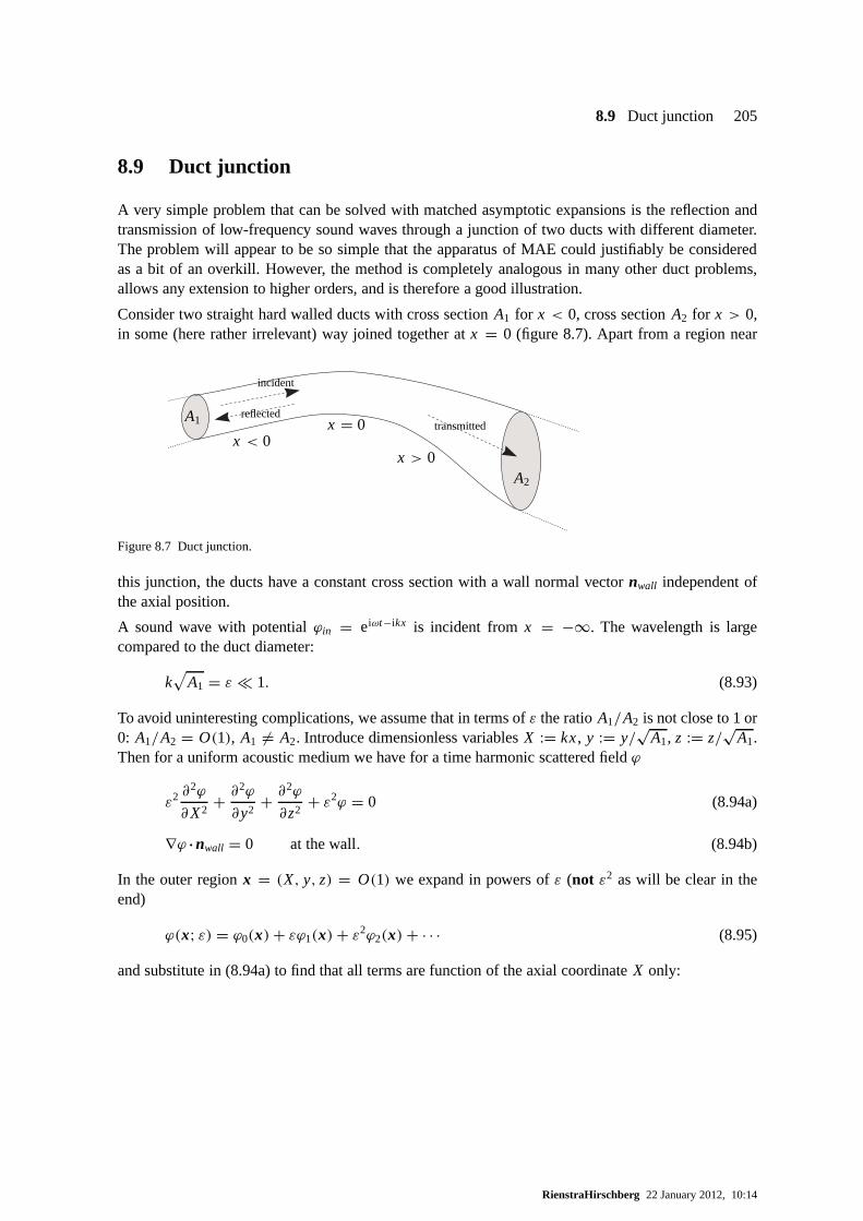
8.9 Duct junction 205
8.9 Duct junction
A very simple problem that can be solved with matched asymptotic expansions is the reflection andtransmission of low-frequency sound waves through a junction of two ducts with different diameter.The problem will appear to be so simple that the apparatus of MAE could justifiably be consideredas a bit of an overkill. However, the method is completely analogous in many other duct problems,allows any extension to higher orders, and is therefore a good illustration.
Consider two straight hard walled ducts with cross sectionA1 for x < 0, cross sectionA2 for x > 0,in some (here rather irrelevant) way joined together atx = 0 (figure 8.7). Apart from a region near
A1
A2
x = 0x < 0
x > 0
incident
reflectedtransmitted
Figure 8.7 Duct junction.
this junction, the ducts have a constant cross section with awall normal vectornwall independent ofthe axial position.
A sound wave with potentialϕin = eiωt−ikx is incident fromx = −∞. The wavelength is largecompared to the duct diameter:
k√
A1 = ε � 1. (8.93)
To avoid uninteresting complications, we assume that in terms ofε the ratioA1/A2 is not close to 1 or0: A1/A2 = O(1), A1 6= A2. Introduce dimensionless variablesX := kx, y := y/
√A1, z := z/
√A1.
Then for a uniform acoustic medium we have for a time harmonicscattered fieldϕ
ε2 ∂2ϕ
∂X2+ ∂2ϕ
∂y2+ ∂2ϕ
∂z2+ ε2ϕ = 0 (8.94a)
∇ϕ ·nwall = 0 at the wall. (8.94b)
In the outer regionx = (X, y, z) = O(1) we expand in powers ofε (not ε2 as will be clear in theend)
ϕ(x; ε) = ϕ0(x)+ εϕ1(x)+ ε2ϕ2(x)+ · · · (8.95)
and substitute in (8.94a) to find that all terms are function of the axial coordinateX only:
RienstraHirschberg 22 January 2012, 10:14

206 8 Approximation methods
O(1) :∂2ϕ0
∂y2+ ∂2ϕ0
∂z2= 0
∇ϕ0·nwall = 0
−→ ϕ0 = ϕ0(X), (8.96a)
O(ε) :∂2ϕ1
∂y2+ ∂2ϕ1
∂z2= 0
∇ϕ1·nwall = 0
−→ ϕ1 = ϕ1(X), (8.96b)
O(ε2) :
∂2ϕ2
∂y2+ ∂2ϕ2
∂z2+ ∂2ϕ0
∂X2+ ϕ0 = 0
∇ϕ2·nwall = 0
−→ϕ2 = ϕ2(X),
∂2ϕ0
∂X2+ ϕ0 = 0.
(8.96c)
This last result is obtained from integration over a cross section Adef== {X = constant} with surface
|A|, and applying Gauss’ theorem
∫
A
(∂2ϕ2
∂y2+ ∂2ϕ2
∂z2+ ∂2ϕ0
∂X2+ ϕ0
)ds =
∫
∂A(∇ϕ2·nwall)d`+
(∂2ϕ0
∂X2+ ϕ0
)|A| = 0.
Evidently, this process can be continued and we obtain
ϕ0 ={
e−i X +R0 ei X (X < 0)T0 e−i X (X > 0)
(8.97a)
ϕn ={
Rn ei X (X < 0)Tn e−i X (X > 0)
(8.97b)
(wheren > 1). The regionX = O(ε) appears to be a boundary layer, and we introduce
x = X/ε,
8 = ϕ(εx, y, z; ε).
The equation for8 becomes
∂28
∂x2+ ∂28
∂y2+ ∂28
∂z2+ ε28 = 0 (8.98)
∇8·nwall = 0 at the wall. (8.99)
but now with matching conditions forx → −∞ andx → +∞, i.e. X ↑ 0 andX ↓ 0 of the outersolution (8.97a-8.97b):
x → −∞ : 8 ' 1 + R0 + ε(R1 − i x + i x R0)+ ε2(R2 + i x R1 − 12x2 − 1
2x2R0)+ · · · ,x → +∞ : 8 ' T0 + ε(T1 − i xT0)+ ε2(T2 − i xT1 − 1
2x2T0)+ · · · .
RienstraHirschberg 22 January 2012, 10:14
8.9 Duct junction 207
Guided by the behaviour under matching we assume the expansion
8 = 80 + ε81 + ε282 · · · ,
then
O(1) : ∇280 = 0 −→ 80 = constant−→ 1 + R0 = T0 (8.100)
O(ε) : ∇281 = 0 −→ 81 = not necessarily constant.
In general, the solution81 is difficult to obtain. However, if we are for the moment only interested inthe global effects on reflection and transmission, we can again make use of Gauss’ theorem. Considera large volume V , reaching fromx = x1 large negative, tox = x2 large positive (large in variablex but small in variableX, so that we can use the matching conditions). Atx = x1 the surface ofVconsists of a cross sectionA1, and atx = x2 a cross sectionA2. The size ofV is denoted by|V |, thesizes ofA1 andA2 by |A1| and|A2|. We integrate over this volume to obtain:
∫
V∇281 dx = −
∫
A1
∂81
∂xds +
∫
A2
∂81
∂xds = −(−i + i R0)|A1| − i T0|A2| = 0
so that:
1 − R0 = T0|A2||A1|
(8.101)
which, together with equation (8.100), determinesR0 andT0 fully. We continue with theO(ε2) term:
O(ε2) : ∇282 = −80.
Again, to obtain82 is difficult in a general situation, but if we follow the same arguments as for81
we find∫
V∇282 dx = −80|V | =
−∫
A1
∂82
∂xds +
∫
A2
∂82
∂xds = −|A1|(i R1 − x1 − x1R0)+ |A2|(−i T1 − x2T0)
= −T0(x2|A2| − x1|A1| + θ1)
whereθ1 denotes the difference, due to obvious details of the junction geometry, between|V | and thesum of the two duct partsx2|A2| − x1|A1|. The above identity results into
|A1|R1 + |A2|T1 = −i T0θ1. (8.102)
This process can be continued, at least formally. For eachn-th step more and more information ofsolution8n−2 is needed. For example, the next step for83 gives a relation forR1 andT1, andR2 andT2, in terms of the integral (check yourself!)
θ2 =∫
V81 dx −
∫ 0
x1
(R1 − i x + i R0x)dx −∫ x2
0(T1 − i T0x)dx
= i |A1|R2 + i |A2|T2.
Note that the correctionsR1 andT1 are imaginary and therefore appear as a phase shift in the reflectedand transmitted (outer-) waves. So the reflection and transmission amplitudes (i.e. absolute value) aregiven byR0 andT0 up to O(ε2).
RienstraHirschberg 22 January 2012, 10:14
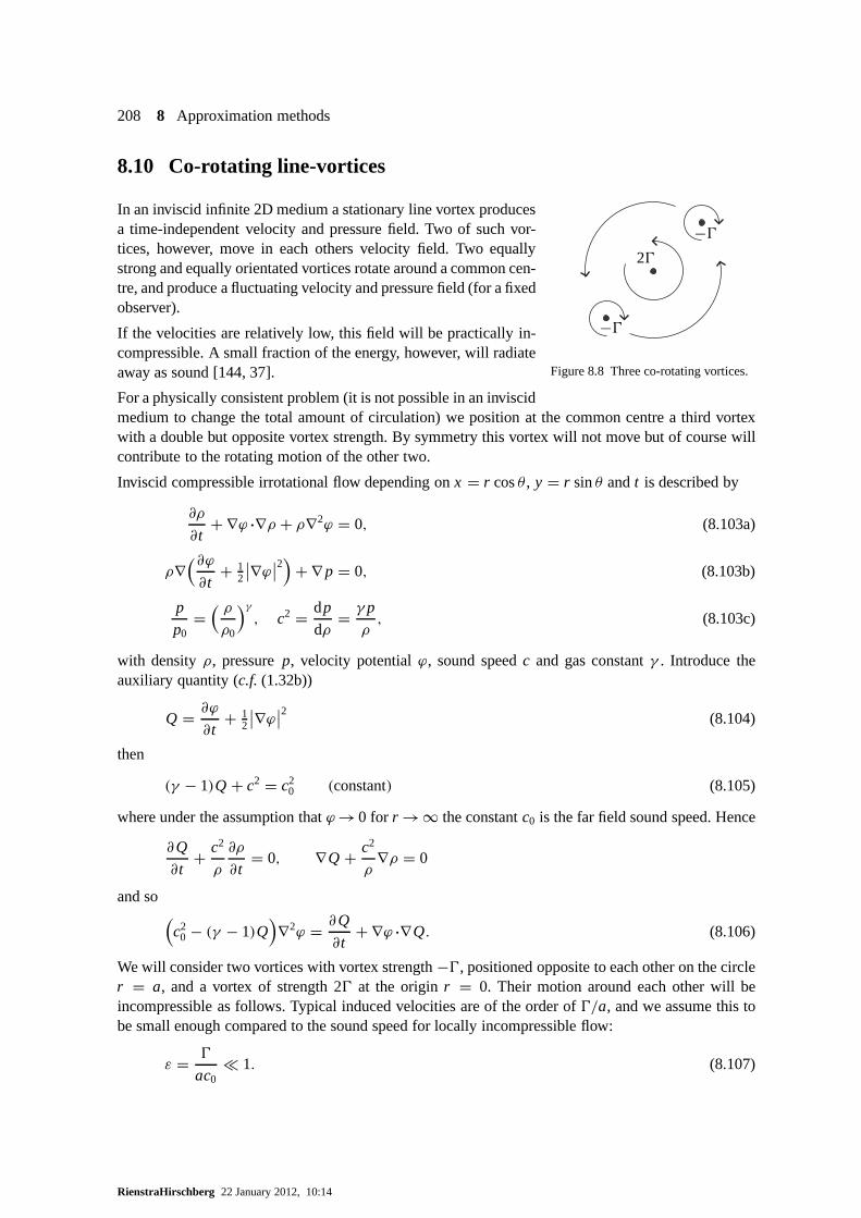
208 8 Approximation methods
8.10 Co-rotating line-vortices
−0
20
−0
Figure 8.8 Three co-rotating vortices.
In an inviscid infinite 2D medium a stationary line vortex producesa time-independent velocity and pressure field. Two of such vor-tices, however, move in each others velocity field. Two equallystrong and equally orientated vortices rotate around a common cen-tre, and produce a fluctuating velocity and pressure field (for a fixedobserver).
If the velocities are relatively low, this field will be practically in-compressible. A small fraction of the energy, however, willradiateaway as sound [144, 37].
For a physically consistent problem (it is not possible in aninviscidmedium to change the total amount of circulation) we position at the common centre a third vortexwith a double but opposite vortex strength. By symmetry thisvortex will not move but of course willcontribute to the rotating motion of the other two.
Inviscid compressible irrotational flow depending onx = r cosθ , y = r sinθ andt is described by
∂ρ
∂t+ ∇ϕ ·∇ρ + ρ∇2ϕ = 0, (8.103a)
ρ∇(∂ϕ∂t
+ 12
∣∣∇ϕ∣∣2
)+ ∇ p = 0, (8.103b)
p
p0=
( ρρ0
)γ, c2 = dp
dρ= γ p
ρ, (8.103c)
with densityρ, pressurep, velocity potentialϕ, sound speedc and gas constantγ . Introduce theauxiliary quantity (c.f. (1.32b))
Q = ∂ϕ
∂t+ 1
2
∣∣∇ϕ∣∣2 (8.104)
then
(γ − 1)Q + c2 = c20 (constant) (8.105)
where under the assumption thatϕ→ 0 for r →∞ the constantc0 is the far field sound speed. Hence
∂Q
∂t+ c2
ρ
∂ρ
∂t= 0, ∇Q + c2
ρ∇ρ = 0
and so(c2
0 − (γ − 1)Q)∇2ϕ = ∂Q
∂t+ ∇ϕ ·∇Q. (8.106)
We will consider two vortices with vortex strength−0, positioned opposite to each other on the circler = a, and a vortex of strength 20 at the originr = 0. Their motion around each other will beincompressible as follows. Typical induced velocities areof the order of0/a, and we assume this tobe small enough compared to the sound speed for locally incompressible flow:
ε = 0
ac0� 1. (8.107)
RienstraHirschberg 22 January 2012, 10:14

8.10 Co-rotating line-vortices 209
Introduce dimensionless variables (where we keep for convenience the same notation):
t := t0/a2, x := x/a, y := y/a, ϕ := ϕ/0, Q := Qa2/02.
Equation (8.106) is then in dimensionless form(1 − (γ − 1)ε2Q
)∇2ϕ = ε2
(∂Q
∂t+ ∇ϕ ·∇Q
). (8.108)
In the inner region r = O(1), we have to leading order the Laplace equation for incompressiblepotential flow
∇2ϕ = 0 (8.109)
with solution the sum6 of the contributions of the three co-rotating vortices
ϕ = 1
πarctan
y
x− 1
2πarctan
y − y1(t)
x − x1(t)− 1
2πarctan
y − y2(t)
x − x2(t). (8.110)
The position vectorx1(t) = (x1(t), y1(t)) (and similarlyx2(t)) is determined by the observation thata vortex is just a property of the flow and therefore the velocity
.x1 (t) must be equal to the induced
velocity of the other vortices atx = x1 :
dx1
dt= 1
2π
y1 − y2
(x1 − x2)2 + (y1 − y2)2− 1
π
y1
x21 + y2
1
(8.111a)
dy1
dt= − 1
2π
x1 − x2
(x1 − x2)2 + (y1 − y2)2+ 1
π
x1
x21 + y2
1
. (8.111b)
From symmetryx2 = −x1. Apart from an irrelevant phase shift the solution along thecircle |x| = 1is given by
x1 = cos(12ωt), y1 = sin(1
2ωt), where ω = 3
2π. (8.112)
Solution (8.110) can now be written as
ϕ = 1
πθ − 1
2πarctan
( r 2 sin 2θ − sinωt
r 2 cos 2θ − cosωt
). (8.113)
For matching with the outer field we need the behaviour of inner solutionϕ for r →∞:
ϕ ' sin(ωt − 2θ)
2πr 2+ · · · (r → ∞). (8.114)
For theouter regionwe first observe that the time scale is dictated by the source,so this is the sameeverywhere. Then, if we scaler = δ(ε)r , it follows from matching with equation (8.114) thatϕ =O(δ2). A significant degeneration of (8.108) is obtained ifδ = ε, when∇2ϕ and∂2ϕ/∂t2 balanceeach other. Together we have:
r = r /ε (8.115a)
ϕ = ε2ϕ (8.115b)
Q = ε2(∂ϕ∂t
+ 12ε
4∣∣∇ϕ
∣∣2)
= ε2Q (8.115c)
6Equation (8.109) is linear.
RienstraHirschberg 22 January 2012, 10:14
210 8 Approximation methods
which gives
(1 − (γ − 1)ε4Q
)∇2ϕ = ∂ Q
∂t+ ε4∇ϕ ·∇ Q (8.116)
To leading order,ϕ satisfies the wave equation
∇2ϕ − ∂2ϕ
∂t2= 0 (8.117)
with outward radiation conditions forr → ∞ (no source at infinity), and a condition of matchingwith (8.114) forr ↓ 0. This matching condition says that, on the scale of the outer solution, the innersolution behaves like a harmonic point source∝ e2iωt at r = 0, with properties to be determined.
Relevant point source solutions are
ϕ = Re{
AH(2)n (ωr )eiωt−inθ
}(8.118)
with H (2)n a Hankel function (Appendix D), and ordern and amplitudeA to be determined. For match-
ing it is necessary that the behaviour forr ↓ 0 coincides with (8.114):
ε2 Re{−A
(n − 1)!
iπ
( 2
ωr
)neiωt−inθ
}∼ sin(ωt − 2θ)
2πr 2(8.119)
(if n > 1). Clearly, there is no other possibility thann = 2, and henceA = −18ω
2. Note that thisorder 2 indicates an acoustic field equivalent to that of a rotating lateral quadrupole. In dimensionalvariables the acoustic far field is given by
ϕ ' 0M3/2
2
( a
πr
)1/2cos
(�(t − r/c0)− 2θ + 1
4π). (8.120)
where frequency� and vortex Mach numberM are given by
� = ω0
a2= 30
2πa2, M = �a
2c0.
We see that for fixedθ the waves radiate outwards (r − c0t constant), for fixedr the waves rotate withpositive orientation (θ− 1
2�t constant), and at a fixed timet the wave crests are localized along spirals(r + 2θc0/� constant). This may be compared with a rotating lawn sprinkler.
The outward radiating time-averaged energy flux or intensity is found from equation (8.120) to be
I = 8
9πρ0c
30M7 a
r. (8.121)
This functional dependence onU7 in 2D is to be compared with theU8-law of Lighthill for turbulencenoise (equation 6.69), and forms a confirmation of the estimates for turbulence in the Lighthill analogy.
We have now obtained the solution to leading order. Higher orders may be constructed in a similarfashion, but we will limit ourselves to the present one. For higher orders more and more equivalentfar fields of higher order multipoles will appear.
We finally note that from a simple calculation the outward radiated 2D power is equal to169 π
2ρ0c30aM7.
Strictly speaking, this amount of energy per time leaks awayfrom the total energy of the system ofvortices (which scales onρ00
2), and we could try to include a small decay in time of the vortexstrength0. This is, however, impossible in the present model.
RienstraHirschberg 22 January 2012, 10:14

8.10 Co-rotating line-vortices 211
Exercises
a) Determine (using Webster’s horn equation) the right-running wavep(x), with p(0) = p0, in an expo-nential horn with radiusa emx.
b) In a hot desert, a man is giving a speech to an audience. The mouth of the man and the ears of theaudience are at a height ofy = h = 1.5 m above the flat ground, given byy = 0. The ground is so hotcompared to the air that a vertically stratified uniform temperature profile is established in the air. Weassume for the region relevant here that this profile corresponds to a sound speed which is linear iny.The sound speed profile is given by:c0(y) = q(1 − εy), whereq = 360 m/s andε = 1
250 m−1. Sincethe sound speed gradient is negative the sound waves are refracted upwards and will disappear into theair. Under the assumptions that the man speaks loud enough, that a typical wave length is small enoughfor ray acoustics to be applicable, and that we only considerrays that skim along the ground, what is thelargest distance over which the man can be heard?
c) Determine the suitable modelling assumptions and derivefrom the wave equations (F.22) and (F.27) thefollowing generalized Webster equations
A−1 d
dx
(∫∫
A
c2 dσdp
dx
)+ ω2p = 0, (8.122)
(ρ0A)−1 d
dx
(Aρ0
dφ
dx
)−
(iω + U
d
dx
)[c−2(iω + U
d
dx
)φ]
= 0. (8.123)
d) A large array of acoustically compact equal Helmholtz resonators (all openings in upward direction)is covered by a top plate of negligible thickness. The plate is solid except for holes positioned exactlyat the openings of the resonator, such that the plate has a uniformporosityσ ∈ (0,1) (= the open fraction). A time harmonic acous-tic field (p, v) eiωt is scattered by plate and Helmholtz resonators.Find an expression for the impedance of the plate surface. You mayassume the model given by equation (5.41), without the nonlinearterms to start with.Hint : you may assume that the neck velocityu′
n = −σ−1(v ·n); use (8.35).
RienstraHirschberg 22 January 2012, 10:14
9 Effects of flow and motion
Being a fluid mechanical phenomenon itself, an acoustic wavemay be greatly affected by mean floweffects like convection, refraction in shear, coupling with vorticity, scattering by turbulence, and manyothers. We will briefly consider here some of these effects.
9.1 Uniform mean flow, plane waves and edge diffraction
Consider a uniform mean flow inx direction with small irrotational perturbations. We have then forpotentialφ, pressurep, densityρ and velocityv the problem given by
∂2φ
∂x2+ ∂2φ
∂y2+ ∂2φ
∂z2− 1
c20
( ∂∂t
+ U0∂
∂x
)2φ = 0,
p = −ρ0
( ∂∂t
+ U0∂
∂x
)φ, p = c2
0ρ, v = ∇φ(9.1)
whereU0, ρ0 andc0 denote the mean flow velocity, density and sound speed, respectively. We assumein the following that|U0| < c0. The equation forφ is known as the convected wave equation.
9.1.1 Lorentz or Prandtl-Glauert transformation
By the following transformation (in aerodynamic context named after Prandtl and Glauert, but quaform originally due to Lorentz)
X = x
β, T = βt + M
c0X, M = U0
c0, β =
√1 − M2, (9.2)
the convected wave equation may be associated to a stationary problem with solutionφ(x, y, z, t) =ψ(X, y, z, T) satisfying
∂2ψ
∂X2+ ∂2ψ
∂y2+ ∂2ψ
∂z2− 1
c20
∂2ψ
∂T2= 0, p = −ρ0
β
( ∂∂T
+ U0∂
∂X
)ψ. (9.3)
For a time harmonic fieldeiωt φ(x, y, z) = ei�T ψ(X, y, z) or φ(x, y, z) = ei K M X ψ(X, y, z), where� = ω/β, k = ω/c0 and K = k/β, we have
∂2ψ
∂X2+ ∂2ψ
∂y2+ ∂2ψ
∂z2+ K 2ψ = 0. (9.4)
The pressure may be obtained fromψ , but sincep satisfies the convected wave equation too, we mayalso associate the pressure field directly by the same transformation with a corresponding stationarypressure field. The results are not equivalent, however, andespecially when the field contains singu-larities some care is in order. The pressure obtained directly is no more singular than the pressure ofthe stationary problem, but the pressure obtained via the potential is one order more singular due tothe convected derivative. See the example below.
9.1 Uniform mean flow, plane waves and edge diffraction 213
9.1.2 Plane waves
A plane wave (inx, y-plane) may be given by
pi = a exp(−i k
x cosθn + y sinθn
1 + M cosθn
)= a exp
(−i kr
cos(θ − θn)
1 + M cosθn
)(9.5)
whereθn is the direction of the normal to the phase plane andx = r cosθ , y = r sinθ . This isphysically not the most natural form, however, becauseθn is due to the mean flow not the directionof propagation. By comparison with a point source field far away, or from the intensity vector (c.f.(F.34,F.35))
〈I〉 = 〈(ρ0v + ρv0)(p/ρ0 + v0·v)〉 = 12ρ0ω
[(β2 Im(φφ∗
x)+ kM|φ|2)ex + Im(φφ∗
y)ey
]
=12ρ0ωk|φ|2
1 + M cosθn
[(cosθn + M)ex + sinθney
]
we can learn thatθs, the direction of propagation (the direction of any shadows, fig. 9.1), is given by
cosθs = M + cosθn√1 + 2M cosθn + M2
, sinθs = sinθn√1 + 2M cosθn + M2
. (9.6)
By introducing the transformed angle2s
cos2s = cosθs√1 − M2 sin2 θs
= M + cosθn
1 + M cosθn, (9.7)
sin2s = β sinθs√1 − M2 sin2 θs
= β sinθn
1 + M cosθn(9.8)
and the transformed polar coordinatesX = Rcos2, y = Rsin2, we obtain the plane wave
pi = a exp(i K M X − i K Rcos(2−2s)
). (9.9)
9.1.3 Half-plane diffraction problem
By using the foregoing transformation, we obtain from the classical Sommerfeld solution for the half-plane diffraction problem (see Jones [97]) of a plane wave (9.9), incident on a solid half plane alongy = 0, x < 0 (fig. 9.1), the following solution (see Rienstra [186]) in terms ofpotential
φ(x, y) = i aβ2
ω(1 − M cos2s)exp
(i K M X − i K R
)(F(0s)+ F(0 s)
)(9.10)
where
F(z) = eiπ/4
√π
eiz2∫ ∞
ze−i t2
dt and 0s, 0s = (2K R)1/2 sin 12(2∓2s). (9.11)
An interesting feature of this solution is the following. When we derive the corresponding pressure
p(x, y) = a exp(i K M X − i K R
)(F(0s)+ F(0 s)
)
+ ae−iπ/4
√π
M cos122s
1 − M cos2sexp
(i K M X − i K R
)sin 1
22( 2
K R
)1/2, (9.12)
RienstraHirschberg 22 January 2012, 10:14

214 9 Effects of flow and motion
θs
Figure 9.1 Sketch of scattered plane wave with mean flow
we see immediately that the first part is a solution by itself:it is a multiple of the solution of thepotential. So the second part has to be a solution too. Furthermore, the first part isregular like φ,while this second part issingularat the scattering edge. As the second part decays for anyR → ∞, itdoes not describe the incident plane wave, and it may be dropped if we do not accept the singularityin p at the edge. So the found solution (9.12) is not unique by the existence of an eigensolutionpv
pv(x, y) = exp(i K M X − i K R
)sin 122√
K R, (9.13)
Without pv, the solution is regular, otherwise it is singular. If we study pv a bit deeper, it transpiresthat it has no continuous potential that decays to zero for large |y|. In fact, pv corresponds to the fieldof vorticity (in the form of a vortex sheet) that is being shedfrom the edge. This may be more clear ifwe construct the corresponding potentialφv for largex, to be compared with (3.65), which is
φv ∼ sign(y)exp(− ω
U0|y| − i
ω
U0x), pv ∼ 0. (9.14)
In conclusion: we obtain the singular solution by transforming the no-flow solution in potential form,
M
0
0.2
0.4
0.6
0.8
1
0.5 1 1.5 2 2.5 3
-0.01
-0.003
0
0.010.1
0.3
1
2
3
4
56
θn
Figure 9.2 (ρ0ω/|a|2)P as function of(M, θn).
and the regular solution from the no-flow solution in pressureform. Their difference is the field of the shed vortex sheet.
This shedding of vorticity costs acoustic energy, so on the onehand it is a sink of acoustic energy. On the other hand, the shedvorticies moving near the solid plate produce also sound, andso the shedding of vorticity is also a source of sound (with themean flow as the unlimited source of energy). The net sum ofboth can be both negative and positive, depending onM andθn.Remarkably, the present model problem allows the followingexact expression of the power absorbed by vortex shedding1.
P = (|a|2/ρ0ω)M cos2 12θn(1 + M cosθn)(2 + 2M cosθn − M) (9.15)
The assumption that just as much vorticity is shed that the pressure field is not singular anymore, isknown as the unsteady Kutta condition. Physically, the amount of vortex shedding is controlled bythe viscous boundary layer thickness compared to the acoustic wave length and the amplitude (and
1This isnot only the energy lost into the vortex sheet, but allacousticenergy lost by vortex shedding. For example, itincludes the irrotational hydrodynamic energy (3.66) associated to the vortex sheet. The energy just lost into the vortex sheetwould beP = (|a|2/ρ0ω)M cos2 1
2θn(1 + M cosθn)(1 + 2M cosθn − M). See Howe [85].
RienstraHirschberg 22 January 2012, 10:14

9.2 Moving point source and Doppler shift 215
the Mach number for high speed flow). These effects are not included in the present acoustic model,therefore they have to be included by an additional edge condition, for example the Kutta condition.As vorticity can only be shed from a trailing edge, a regular solution is only possible ifM > 0. IfM < 0 the edge is a leading edge and we have to leave the singular behaviour as it is.
9.2 Moving point source and Doppler shift
Consider a point (volume) source of strengthQ(t) (the volume flux), moving subsonically along thepathx = xs(t) in a uniform acoustic medium. The generated sound field is described by
1
c20
∂2 p
∂t2− ∇2 p = ρ0
∂
∂t
{Q(t)δ(R(t))
}, R(t) = x − xs(t). (9.16)
Using the free field Green’s function (equation (6.37) or Appendix E)
G(x, t|y, τ ) = 1
4πc20|x − y|
δ(t − τ − |x − y|
c0
),
the solution for potentialϕ, with p = −ρ0∂∂t ϕ, is given by
4πϕ(x, t) = −∫ ∞
−∞
Q(τ )
R(τ )δ(t − τ − R(τ )
c0
)dτ, R = |R|. (9.17)
Using theδ-function integral (C.28)∫ ∞
−∞δ(h(τ ))g(τ )dτ =
∑
i
g(τi )
|h′(τi )|, h(τi ) = 0 (C.28)
this representation is very elegantly2 [52] reduced to the Liénard-Wiechert potential ([99, p.127])
4πϕ(x, t) = − Qe
Re(1 − Me cosϑe), (9.18)
where the subscripte denotes evaluation at timete, given by the equation
c0(t − te)− R(te) = 0. (9.19)
Absolute values are suppressed because we assumed|Me| < 1. Restriction (9.19) is entirely naturaland to be expected. If we trace the observed acoustic perturbation back to its origin, we will find3 itto be created at timete by the source at positionxs(te) and strengthQ(te). Therefore,te is usuallycalledemission time, or retarded time. It is important to note that by its implicit definition (9.19), te isa function of botht andx.
Other convenient notations used here and below are
M = x′s/c0, M = |M|, RM cosϑ = R ·M,
2To appreciate the elegance the reader might compare it with the more traditional derivation as found in [143, p.721] forthe less general problem of a point source moving with constant speed along a straight line.
3A generalization to supersonic motion of the source involves in general a summation, according to (C.28), over morethan one solution of equation (9.19).
RienstraHirschberg 22 January 2012, 10:14

216 9 Effects of flow and motion
whereM and M are, respectively, the scalar and vectorial Mach number of the source, whileϑ isthe angle between the source velocity vector and the observer’s position, seen from the source. ThecombinationM cosϑ is often also denoted byMr .
By applying the chain rule to equation (9.19) we obtain the identities
∂te∂t
= 1
1 − Me cosϑe,
∂Re
∂t= − c0Me cosϑe
1 − Me cosϑe,
∂
∂t(ReMe cosϑe) = Re·M ′
e − c0M2e
1 − Me cosϑe.
After differentiation of equation (9.18) with respect to time, we finally have
4πp(x, t) = ρ0Q′e
Re(1 − Me cosϑe)2+ ρ0Qe
Re·M ′e + c0Me(cosϑe − Me)
R2e(1 − Me cosϑe)3
. (9.20)
The O(R−1e )-part dominates the far field, while theO(R−2
e )-part dominates the near field [123]. Atypical effect of motion is that both the pressure and the potential fields are increased by the “Dopplerfactor” (1− Me cosϑe)
−1, but not with the same power. Furthermore, more Doppler factors appear forhigher order multipole sources. (See Crighton [38].)
The name “Doppler factor” is due to its appearance in the well-known frequency shift of movingharmonic sources. Assume
Q(t) = Q0 eiω0t
with frequencyω0 so high that we candefinean instantaneous frequencyω for an observer of (9.20)at positionx:
ω(t) = d
dt(ω0te) = ω0
1 − Me cosϑe. (9.21)
This describes theDoppler shiftof frequencyω0 due to motion. Expression (9.20) is quite general.The more common forms are for a straight source path with constant velocityxs(t) = (V t,0,0) inwhich caseMe is constant andx′′
s = 0.
Analogous to the above point volume source, or monopole, we can deduce the field of a moving pointforce, or dipole. For this we return to the original linearized gas dynamics equations inρ, v, and pwith external forceF(t)δ(x − xs(t)), and eliminateρ andv to obtain:
1
c20
∂2 p
∂t2− ∇2 p = −∇ ·
{F(t)δ(R(t))
}. (9.22)
Following the same lines as in the monopole problem we have the solution
4πp(x, t) = −∇ ·( Fe
Re(1 − Me cosϑe)
)(9.23)
Here we see that a rotating force is not the same as a rotating∇ · F -field, sincete = te(x, t). Byapplication of the chain rule to equation (9.19) we derive:
∇Re = −c0∇te = Re
Re(1 − Me cosϑe),
∇(ReMe cosϑe) = Me − Re
Re(1 − Me cosϑe)
( Re·M ′e
c0− M2
e
),
RienstraHirschberg 22 January 2012, 10:14

9.3 Rotating monopole and dipole with moving observer 217
so that we have the general expression for a moving point force:
4πp(x, t) = Re· F′e − c0Me·Fe
c0R2e(1 − Me cosϑe)
2+ (Re·Fe)
Re·M ′e + c0(1 − M2
e)
c0R3e(1 − Me cosϑe)
3. (9.24)
The O(R−1e )-part dominates the far field, while theO(R−2
e )-part dominates the near field [123].
It should be noted that the above distinction between a pointsourceQ and a point forceF is ratheridealized. In any real situationQ andF are coupled, since in general a real mass source also producesa momentum change (see [52]).
9.3 Rotating monopole and dipole with moving observer
An application of the previous section is a model for (subsonic) propeller noise, due to Succi andFarassat [61, 223].
Two main sources of sound may be associated to a moving propeller blade: the displacement of fluidby the moving body leading to thickness noise, and the movinglift force distribution leading to loadingnoise. See the next section 9.4, equation (9.28). A description of the loading noise is obtained byrepresenting the propeller blade force by an equivalent distribution of point forcesF j , followed by asummation overj of the respective sound fields given by equation (9.24).
The thickness noise is a bit more involved. It can be shown (equation 9.32) that a compact movingbody of fixed volumeV generates a sound field, due to its displacement of fluid, given by thetimederivativeof equation (9.16) whileQ = V , with solution thetime derivativeof equation (9.20).
4πpth(x, t) = ρ0V∂2
∂t2
1
Re(1 − Me cosϑe).
(Equivalent forms in terms of spatial derivatives are also possible; see for example [24, 61].) Bydiscretising the propeller blade volume by an equivalent collection of volumesVj , the thickness noiseis found by a summation overj of the respective sound fields.
The method is attractive in its relative simplicity, and easy programming. The formulas are laborious,however. Therefore, to illustrate the method, we will work out here the related problems of the farfield of a subsonically rotating and translating monopoleQ = q0 and dipole f0. The position of thepoint source, rotating in thex, y-plane along a circle of radiusa with frequencyω, and translatingalong thez-axis with constant velocityU (figure 9.3), is given by
xs(t) = (a cosωt,a sinωt,Ut).
It is practically of most interest to consider an observer moving with the source, with forward speedUt . Therefore, we start with the field of the source, given in thestationary medium by equation (9.20),and substitute for position vectorx the position of a co-moving observerxo = (xo, yo, zo), given inspherical coordinates by
xo(t) = (r cosφ sinϑ, r sinφ sinϑ, r cosϑ + Ut).
With R(o)e = xo(t)− xs(te) we obtain the relations
R(o)e ·Me = MR r sinϑ sin(φ − ωte)+ MF r sinϑ + M2
F R(o)e ,
R(o)e ·M ′
e = c0M2R
(1 − r
asinϑ cos(φ − ωte)
),
M2e = M2
R + M2F , where MR = ωa/c0, MF = U/c0.
RienstraHirschberg 22 January 2012, 10:14

218 9 Effects of flow and motion
x
yz
Figure 9.3 Trajectory of point, moving along helical pathxs(t).
The “far field” denotes the asymptotic behaviour for(a/r ) → 0. Since
c20(t − te)
2 = (R(o)e )2 = r 2 − 2ar sinϑ cos(φ − ωte)+ a2 + 2Ur (t − te) cosϑ + U2(t − te)2
and noting that asymptoticallyt − te = O(r/c0), we have fora/r → 0
te = t − r
c0+ a
c0sinϑ cos(φ − ωt + kr )+ . . .
wherek = ω/c0 and
r = rMF cosϑ +
√1 − M2
F sin2ϑ
1 − M2F
, a = a1√
1 − M2F sin2ϑ
.
With this we find:
R(o)e ' r − a sinϑ cos(φ − ωt + kr )
Me cosϑe '(1 − M2
F )MR sinϑ sin(φ − ωt + kr )+ MF cosϑ + M2F
√1 − M2
F sin2ϑ
MF cosϑ +√
1 − M2F sin2ϑ
Altogether in equation (9.20):
4πp(x, t) = ρ0c0q0
R2e(1 − Me cosϑe)
3
( (R(o)e ·M ′
e
c0+ Me cosϑe − M2
e
)
' −ρ0c0q0
ar
(1 − M2F )
2M2R sinϑ cos(φ − ωt + kr )
(MF cosϑ +
√1 − M2
F sin2ϑ)2(
1 − Me cosϑe
)3 (9.25)
We do have aO(1/r ) decay, and in spite of the dQ(t)/dt = 0, a nearly harmonic signal. Note the2-lobe radiation pattern,i.e. 2 maxima perpendicular to the axis of rotation where sinϑ = 1, andminima in the direction of the axis where sinϑ = 0.
RienstraHirschberg 22 January 2012, 10:14
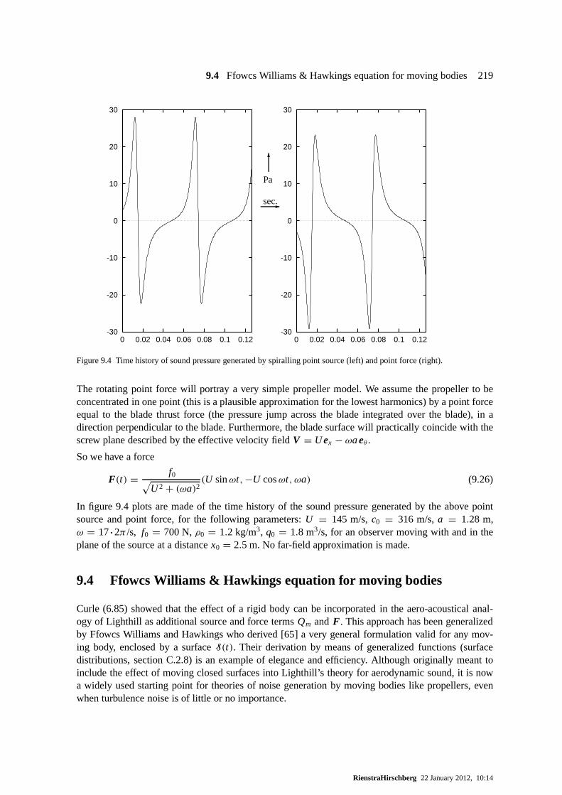
9.4 Ffowcs Williams & Hawkings equation for moving bodies 219
-30
-20
-10
0
10
20
30
0 0.02 0.04 0.06 0.08 0.1 0.12-30
-20
-10
0
10
20
30
0 0.02 0.04 0.06 0.08 0.1 0.12
Pa
6
sec.-
Figure 9.4 Time history of sound pressure generated by spiralling point source (left) and point force (right).
The rotating point force will portray a very simple propeller model. We assume the propeller to beconcentrated in one point (this is a plausible approximation for the lowest harmonics) by a point forceequal to the blade thrust force (the pressure jump across theblade integrated over the blade), in adirection perpendicular to the blade. Furthermore, the blade surface will practically coincide with thescrew plane described by the effective velocity fieldV = U ex − ωaeθ .
So we have a force
F(t) = f0√U2 + (ωa)2
(U sinωt,−U cosωt, ωa) (9.26)
In figure 9.4 plots are made of the time history of the sound pressure generated by the above pointsource and point force, for the following parameters:U = 145 m/s,c0 = 316 m/s,a = 1.28 m,ω = 17·2π /s, f0 = 700 N,ρ0 = 1.2 kg/m3, q0 = 1.8 m3/s, for an observer moving with and in theplane of the source at a distancex0 = 2.5 m. No far-field approximation is made.
9.4 Ffowcs Williams & Hawkings equation for moving bodies
Curle (6.85) showed that the effect of a rigid body can be incorporated in the aero-acoustical anal-ogy of Lighthill as additional source and force termsQm and F. This approach has been generalizedby Ffowcs Williams and Hawkings who derived [65] a very general formulation valid for any mov-ing body, enclosed by a surfaceS(t). Their derivation by means of generalized functions (surfacedistributions, section C.2.8) is an example of elegance andefficiency. Although originally meant toinclude the effect of moving closed surfaces into Lighthill’s theory for aerodynamic sound, it is nowa widely used starting point for theories of noise generation by moving bodies like propellers, evenwhen turbulence noise is of little or no importance.
RienstraHirschberg 22 January 2012, 10:14
220 9 Effects of flow and motion
There is no unique relation between a source and its sound field, because a given field can be createdby infinitely many equivalent but different sources (section 2.6.1). Therefore, there is no unique wayto describe the effect of a surfaceS(t) in terms of an acoustic source distribution, and a simple andtransparent choice is preferable. The choice put forward byFfowcs Williams and Hawkings was bothsimple and transparent: just force any flow variable to vanish inside the enclosed volume. The resultingequations are automatically valid everywhere, and use can be made of the free field Green’s function.
Consider a finite volumeV = V(t) with sufficiently smooth surfaceS = S(t), moving continuouslyin space. Introduce a (smooth) functionf (x, t) such that
f (x, t)
< 0 if x ∈ V(t),
= 0 if x ∈ S(t),
> 0 if x 6∈ V(t),
but otherwise arbitrary. If we multiply any physical quantity by the Heaviside functionH ( f ) – suchasρ ′ H ( f ) – we obtain a new variable which vanishes identically withinV becauseH ( f ) = 1 inthe fluid, andH ( f ) = 0 insideV. Since∇ f | f =0 is directed normal outwards fromV, the outwardnormaln of S is given by (section A.3).
n(x, t) = ∇ f
|∇ f |
∣∣∣∣f =0
.
Let the surfaceS(t) be parametrized in time and space, by coordinates4 (t;λ,µ). A surface pointxS(t) ∈ S (considerλ andµ fixed), moving with velocityU = .
xS, remains at the surface for all time,so f (xS(t), t) = 0 for all t , and therefore
∂ f
∂t= − .
xS ·∇ f = −(U ·n)|∇ f |.
It is important to note that the normal velocity(U ·n) is a property of the surface, and is independentof the choice off or parametrization. We now start the derivation by multiplying the exact equations(1.1,1.2) of motion for the fluid byH ( f ):
H ( f )[∂ρ ′
∂t+ ∇ ·(ρv)
]= 0,
H ( f )[ ∂∂t(ρv)+ ∇ ·(P + ρvv)
]= 0,
whereρ ′ = ρ − ρ0 andρ0 is the mean level far away from the body. Although the original equationswere only valid outside the body, the new equations are trivially satisfied insideV, and so they are valideverywhere. By reordering the terms, and using the identity∂
∂t H ( f ) = −U ·∇H ( f ), the equationscan be rewritten as equations for the new variablesρ ′H ( f ) andρvH ( f ) as follows.
∂
∂t[ρ ′H ( f )] + ∇·[ρvH ( f )] = [ρ0U + ρ(v − U)]·∇H ( f ),
∂
∂t[ρvH ( f )] + ∇·[(ρvv + P)H ( f )] = [ρv(v − U)+ P]·∇H ( f ).
4WhenS(t) is the surface of a solid and undeformable body, it is naturalto assume a spatial parametrization which ismaterially attached to the surface. This is, however, not necessary. Like the auxiliary functionf , this parametrization is notunique, but that will appear to be of no importance.
RienstraHirschberg 22 January 2012, 10:14

9.4 Ffowcs Williams & Hawkings equation for moving bodies 221
Using the same procedure (subtracting the time-derivativeof the mass equation from the divergenceof the momentum equation) as for Lighthill’s analogy (2.65), we find the Ffowcs Williams-Hawkingsequations [65]:
∂2
∂t2ρ ′H ( f )− c2
0∇2ρ ′ H ( f ) = ∇·∇·
[(ρvv − τ + (p′ − c2
0ρ′) I
)H ( f )
]
+ ∂
∂t
[(ρ(v − U)+ ρ0U
)·∇H ( f )
]− ∇·
[(ρv(v − U)+ p′ I − τ
)·∇H ( f )
]. (9.27)
The sources at the right hand side consist of the double divergence of the common quadrupole-typeLighthill stress tensor, and a time derivative and divergence of sources only present at the surfacef = 0. Of course, the right hand side contains all the unknowns, and in principle this equation (9.27)is not simpler to solve than the original Navier-Stokes equations. However, as with Lighthill’s analogy,the source terms are of aerodynamic nature, and can be solvedseparately, without including the verysmall acoustic back-reaction.
Very often, Lighthill’s stress tensorρvv − τ + (p′ − c20ρ
′) I and the shear stresses at the surface arenegligible. Moreover, if the surfaceS is solid such thatv ·n = U ·n, and we change from densityto pressure as our field variable, and definep ′ = p′ H ( f ), we have a reduced form of the FfowcsWilliams-Hawkings equation, which is widely used for subsonic propeller and fan noise (no shocks)[61]
1
c20
∂2
∂t2p ′ − ∇2 p ′ = ∂
∂t
[ρ0U ·n|∇ f |δ( f )
]− ∇·
[p′n|∇ f |δ( f )
]. (9.28)
The first source term is of purely geometrical nature, and describes the noise generated by the fluiddisplaced by the moving body. The associated field is called thickness noise. The second part dependson the normal surface stresses due to the pressure distribution, and describes the noise generated bythe moving force distribution. The associated field is called loading or lift noise.
If we know the pressure distribution along the surface, we can in principle solve this equation, in a waysimilar to the problem of the moving point source of section 9.2. Let us consider first the followingprototype problem
1
c20
∂2
∂t2ϕ − ∇2ϕ = Q(x, t)|∇ f |δ( f ). (9.29)
By using the free field Green’s function we can write
4πϕ(x, t) =∫ ∫∫∫
Q(y, τ )R
δ(t − τ − R/c0)|∇ f |δ( f )dy dτ,
whereR = |x − y(τ )|, the distance between observer’s and source’s position. Noting that|∇ f |δ( f )is just equivalent to the surface distribution ofS(t) (equation C.38), we can integrateδ( f ) (equationC.37 or C.39) and write
4πϕ(x, t) =∫ ∫∫
S(t)
Q(y, τ )R
δ(t − τ − R/c0)dσ dτ.
The integral overτ can be evaluated by noting that any contributions come from the solutionτ = teof the emission-time equation (the zero of the argument of the remainingδ-function), given by
c0(t − τ)− R = 0,
RienstraHirschberg 22 January 2012, 10:14
222 9 Effects of flow and motion
which describes (for givenx, t) a surface in(y, τ )-space, symbolically denoted byS(te). Analogousto the point source field (9.18) we have then
4πϕ(x, t) =∫∫
S(te)
Qe
Re(1 − Me cosϑe)dσ. (9.30)
As before, subscripte denotes evaluation at emission timete, andM cosϑ is the component of thevectorial Mach number of the source in the direction of the observer (in some literature also denotedby Mr ). From this auxiliary solution we can now formulate a solution for p ′ as follows
4π p ′(x, t) = ∂
∂t
∫∫
S(te)
ρ0Ue·ne
Re(1 − Me cosϑe)dσ − ∇·
∫∫
S(te)
pene
Re(1 − Me cosϑe)dσ. (9.31)
Extreme care should be taken in interpreting this equation,because for anyx andt the emission timete varies over the source region, while at the same time the source varies its position! Other formsof the solution are available which might be easier to handlein certain applications; seee.g.Farassat[60, 61].
It is therefore interesting to consider the compact limit, in which case the typical wave length is muchlonger than the body size. The emission time does not vary significantly over the source region, andRe andMe cosϑe refer only to a single typical source coordinatexs, for example the centre of gravity.The source becomes equivalent to a point source (section 9.2,9.3).
A particularly interesting form (Farassat [61]) for the thickness noise component is found by writingthe surface integral as a volume integral. Using
ρ0U ·n|∇ f |δ( f ) = ∂
∂tρ0(1 − H ( f )),
and noting that the function 1− H ( f ) equals unity inside the bodyV and zero elsewhere, we havefor the thickness noise component of equation (9.31)
∂
∂t
∫∫
S(te)
ρ0Ue·ne
Re(1 − Me cosϑe)dσ = ∂2
∂t2
∫∫∫
V(te)
ρ0
Re(1 − Me cosϑe)dy.
Since the volume integral of the constant 1 is justV , the volume ofV, and denoting the total force ofthe fluid on the body by
F(t) =∫∫
S(t)
p·n dσ,
we have the compact limit of equation (9.31) (see also section 9.3)
4π p ′(x, t) ' ∂2
∂t2
( ρ0V
Re(1 − Me cosϑe)
)− ∇·
( Fe
Re(1 − Me cosϑe)
). (9.32)
Exercises
a) Evaluate the expressions for the acoustic field of the propeller of equation 9.26 without forward speed(U = 0) and find the approximation for the far field. What can you tell about the typical lobes in theradiation pattern?
b) Evaluate the expressions for the acoustic field of a movingpoint volume source (9.20) and point force(9.24) for the windtunnel situation: a moving sourcexs = V t ex and a moving observex = a + V t ex.
RienstraHirschberg 22 January 2012, 10:14
A Integral laws and related results
A.1 Reynolds’ transport theorem
Conservation laws such as mass conservation are understoodmost easily when they are applied to avolume V = V(t) (enclosed by the surfaceS = S(t)) which is contained in the fluid. We call thisa material volume. The concept arises when considering a fluid particle which is large in number ofmolecules, but small compared to the macroscopic scales in the problem. For a certain –diffusioncontrolled– period of time the particle keeps its identity,and can be labelled.
For an arbitrary single-valued scalar functionF = F(xi , t) (denoting any property of the fluid) withcontinuous derivatives the following integral relation holds:
d
dt
∫∫∫
V
F dx =∫∫∫
V
(DF
Dt+ (∇·v)F
)dx =
∫∫∫
V
∂F
∂tdx +
∫∫
S
Fv ·n dσ. (A.1)
This theorem, known as Reynolds’ Transport Theorem (see equation C.40), is used to translate integralconservation laws into differential conservation laws.
A.2 Conservation laws
The conservation laws (mass, momentum, energy) in integralform are more general than in differ-ential form because they can be applied to flows with discontinuous properties. We will give here asummary of the basic formulae. A detailed derivation may be found in [166] or [226].
Mass conservation (F = ρ):
d
dt
∫∫∫
V
ρ dx = 0. (A.2)
Momentum conservation (F = ρvi ):
d
dt
∫∫∫
V
ρvi dx =∫∫∫
V
fi dx −∫∫
S
Pi j n j dσ. (A.3)
Energy conservation (F = ρ(e+ 12v
2), v2 = vivi ):
d
dt
∫∫∫
V
ρ(e+ 12v
2)dx =∫∫∫
V
f ivi dx −∫∫
S
Pi j v j ni dσ −∫∫
S
qi ni dσ. (A.4)
For an arbitrary control volumeV∗(t) with surfaceS∗(t), and whereb is the local velocity ofS∗,Reynolds’ theorem becomes:
d
dt
∫∫∫
V∗
F dx =∫∫∫
V∗
∂F
∂tdx +
∫∫
S∗
Fbi ni dσ. (A.5)
224 A Integral laws and related results
Applying (A.2) and (A.5) withF = ρ we find:
d
dt
∫∫∫
V∗
ρ dx =∫∫∫
V∗
∂ρ
∂tdx +
∫∫
S∗
ρbi ni dσ (A.6)
∫∫∫
V
∂ρ
∂tdx = −
∫∫
S
ρvi ni dσ. (A.7)
At a given instantV∗ coincides with a given material volumeV, hence (A.7) can be used to eliminatethe first integral on the right-hand side of (A.6) to obtain:
d
dt
∫∫∫
V∗
ρ dx =∫∫
S∗
ρ(bi − vi )ni dσ. (A.8)
This can be applied to any volumeV∗ and in particular to a fixed volume (bi = 0). In a similar waywe have for the momentum:
d
dt
∫∫∫
V∗
ρvi dx +∫∫
S∗
ρvi (v j − b j )n j dσ =∫∫∫
V∗
fi dx −∫∫
S∗
Pi j n j dσ (A.9)
and for the energy:
d
dt
∫∫∫
V∗
ρ(e+ 12v
2)dx +∫∫
S∗
ρ(e+ 12v
2)(vi − bi )ni dσ
=∫∫∫
V∗
fivi dx −∫∫
S∗
Pi j v j ni dσ −∫∫
S∗
qi ni dσ. (A.10)
For the entropys we further find:
d
dt
∫∫∫
V∗
ρsdx +∫∫
S∗
ρs(vi − bi )ni dσ +∫∫
S∗
1
Tqi ni dσ > 0 (A.11)
where the equality is valid when the processes in the flow are reversible.
A.3 Normal vectors of level surfaces
A convenient way to describe a smooth surfaceS is by means of a suitable smooth functionS(x),wherex = (x, y, z), chosen such that the level surfaceS(x) = 0 is just equivalent toS. SoS(x) = 0if and only if x ∈ S.
Consider a pointx0 and a neighbouring pointx0 + h, both on the surfaceS. ExpandS(x0 + h) into aTaylor series inh. We then obtain
S(x0 + h) = S(x0)+ h·∇S(x0)+ O(h2) ' h·∇S(x0) = 0.
Since in the limit for|h| → 0 the vector∇S(x0) is normal to the tangent vectorh, it is normal to thesurfaceS. Furthermore, the unit normal vectornS = ∇S
|∇S| (at S = 0) is directed from theS< 0-sideto theS> 0-side.
If we expandS(x) nearx0 ∈ S we haveS(x) = (x − x0)·∇S(x0) + . . . , so, near the surface,S(x)varies, to leading order, only in the coordinate normal to the surface.
RienstraHirschberg 22 January 2012, 10:14

B Order of magnitudes: O and o.
In many cases it is necessary to indicate in a compact way the behaviour of some functionf (x), ofvariable or parameterx, asx tends to some limit (finite or infinite). The usual way to do this is bycomparing with a simpler functiong(x). For this we have theorder symbols Oando. When f iscomparable with or dominated byg, we have
Definition B.1 f (x) = O(g(x)) as x→ a
means, that there is a constant C and an interval(a − h,a + h)such that for all x∈ (a − h,a + h): | f (x)| 6 C|g(x)|.
Whenx ↓ a the interval is one-sided:(a,a + h); similarly for x ↑ a. For the behaviour at infinity wehave
Definition B.2 f (x) = O(g(x)) as x→ ∞means, that there is a constant C and an interval(x0,∞)
such that for all x∈ (x0,∞): | f (x)| 6 C|g(x)|.
Similarly for x → −∞. When f is essentially smaller thang we have
Definition B.3 f (x) = o(g(x)) as x→ a
means, that for every positiveδ there is an interval(a − η,a + η)
such that for all x∈ (a − η,a + η): | f (x)| 6 δ|g(x)|.
with obvious generalizations tox ↓ a, x → ∞, etc.
Theorem B.1 If limf (x)
g(x)exists, and is finite, then f(x) = O(g(x)).
Theorem B.2 If limf (x)
g(x)= 0, then f(x) = o(g(x)).
Note that f = o(g) implies f = O(g), in which case the estimateO(g) is only an upper limit, andnot as informative as the “sharpO”, defined by
Definition B.4 f (x) = Os(g(x)) means: f(x) = O(g(x)) but f(x) 6= o(g(x).
C Fourier transforms and generalized functions
C.1 Fourier transforms
The linearity of sound waves allows us to build up the acoustic field as a sum of simpler solutions ofthe wave equation. The most important example is the reduction into time harmonic components, orFourier analysis. This is attractive in several respects. Mathematically, because the equation simplifiesgreatly if the coefficients in the wave equation are time-independent, and physically, because theFourier spectrum represents the harmonic perception of sound.
Consider a functionp(t) with the following (sufficient, not necessary) conditions [28, 98, 119, 168,248].
– p is continuous, except for at most a finite numberof discontinuities wherep(t) = 1
2[p(t + 0)+ p(t − 0)].– |p(t)| and|p(t)|2 are integrable.
Then theFourier transform p(ω) of p(t) is defined as the complex function
p(ω) = Fp(ω)def== 1
2π
∫ ∞
−∞p(t) e−iωt dt, (C.1)
while according to Fourier’s inversion theorem,p(t) is equal to the inverse Fourier transform
p(t) = F −1p (t)
def==∫ ∞
−∞p(ω) eiωt dω. (C.2)
The Fourier transform and its inverse are closely related. Apart from a sign change and a factor 2π , itis the same operation:F −1
p (t) = 2πF p(−t). It is important to note that slight differences with respectto the factor 1/2π , frequencyω = 2π f , and the sign of the phase iωt are common in the literature.Especially the prevailinge±iωt -convention shouldalwaysbe checked when referring or comparing toother work.
Some examples of Fourier transforms are:
1
2π
∫ ∞
−∞H (t) e−αt e−iωt dt = 1
2π(α + iω), (C.3a)
1
2π
∫ ∞
−∞
H (t)√t
e−αt e−iωt dt = 1
2√π
√α + iω
, (C.3b)
1
2π
∫ ∞
−∞
1
1 + t2e−iωt dt = 1
2e−|ω|, (C.3c)
1
2π
∫ ∞
−∞e− 1
2 t2e−iωt dt = 1√
2πe− 1
2ω2, (C.3d)
C.1 Fourier transforms 227
whereα > 0, the ordinary square root is taken, andH (t) denotes Heaviside’s unit step function(C.29), which isH (t) = 1 for t > 0 andH (t) = 0 for t < 0.
Although it may seem to be no serious restriction to assume that a physically relevant signalp(t)vanishes att = ±∞, we deal in practice with simplified models, yielding expressions forp(t) whichdo not decay at infinity (e.g.a constant, sin(ω0t)). So we have on the one hand the “real”p(t) whichis Fourier-transformable, and on the other hand the approximate “model” p(t), which is not alwaysFourier-transformable. Is there a way to approximate, or atleast get an idea of, the real Fourier trans-form, using the approximatep(t)? One way is to assumep to vanish outside a certain large interval[−N, N], as for example:
1
2π
∫ N
−Ne−iωt dt = sinωN
πω
1
2π
∫ N
−Nsin(ω0t) e−iωt dt = i
2π
(sin(ω0 + ω)N
ω0 + ω− sin(ω0 − ω)N
ω0 − ω
)
We see a large maximum (∼ N/π ) depending onN near the dominating frequencies, and for theother frequencies an oscillatory behaviour, also depending on N, that is difficult to interpret. This istoo vague and too arbitrary for general use. Therefore, a mathematically more consistent and satisfyingapproach, not depending on the arbitrary choice of the interval size, will be introduced later in termsof generalized functions.
Derivative
Since a derivative tot corresponds to a multiplication by iω as follows
d
dtp(t) =
∫ ∞
−∞iω p(ω) eiωt dω, (C.4)
the wave equation reduces to the Helmholtz equation
∇2ϕ − 1
c2
∂2ϕ
∂t2= 0
F.T.=⇒ ∇2ϕ + ω2
c2ϕ = 0. (C.5)
Further reduction is possible by Fourier transformation inspace variables.
More dimensions and Hankel transform
Fourier transforms inn space dimensions is usually denoted as
f (k) =∫
Rn
f (x)eik·x dx, f (x) = 1
(2π)n
∫
Rn
f (k)e−ik·x dk. (C.6)
The Hankel transformHm( f ;ρ) of a functionφ(r ), given by
Hm(φ;ρ) =∫ ∞
0φ(r )Jm(ρr )r dr (C.7)
RienstraHirschberg 22 January 2012, 10:14
228 C Fourier transforms and generalized functions
arises naturally when the 2D Fourier transform of a functionf (x) is re-written in polar coordinates.
f (k) =∫∫
R2
f (x)eik·x dx =∞∑
m=−∞eimα Hm( fm;ρ) (C.8)
wherex = (r cosϑ, r sinϑ), k = (ρ sinα, ρ cosα),
f (x) = 1
2π
∞∑
m=−∞fm(r )e−imϑ
and use is made of equation (D.62).
Multiplication and convolution
Fourier transformation is basically a linear operation andlittle can be said about other than linearcombinations of transformed functions. Only for multiplication with powers ofω we have
∫ ∞
−∞(iω)n p(ω) eiωt dω = dn
dtnp(t). (C.9)
For multiplication with a generalq(ω) we find the convolution product ofp(t) andq(t), also knownas the Convolution Theorem
(p∗q)(t) = 1
2π
∫ ∞
−∞p(t ′)q(t − t ′)dt ′ =
∫ ∞
−∞p(ω)q(ω) eiωt dω. (C.10)
Note that in terms of generalized functions, to be introduced below, result (C.9) for the product withωn is a special case of the convolution theorem. A particular case is Parseval’s theorem, obtained bytaking1 q(t ′) = p∗(−t ′) andt = 0:
∫ ∞
−∞| p(ω)|2 dω = 1
2π
∫ ∞
−∞|p(t ′)|2 dt ′ (C.11)
which is in a suitable context a measure of the total energy ofa signalp(t).
Poisson’s summation formula
Intuitively, it is clear that the high frequencies relate tothe short time behaviour, and the low fre-quencies to the long time behaviour. An elegant result due toPoisson is making this explicit.
∞∑
n=−∞p(λn) = 2π
λ
∞∑
n=−∞p(2πn
λ
). (C.12)
Sampling with large steps (λ large) of p yields information about the low part of the spectrum andvice versa.
1z∗ = x − i y denotes the complex conjugate ofz = x + i y.
RienstraHirschberg 22 January 2012, 10:14
C.1 Fourier transforms 229
Reality condition
Although p(ω) is complex, the correspondingp(t) is in any physical context real. Therefore, not anyp(ω) can occur. A givenp(ω) corresponds to a real signalp(t) if it satisfies thereality condition
p(−ω) = p(ω)∗. (C.13)
This is just the consequence ofp(t), given by equation (C.2), being identically equal to its complexconjugate.
C.1.1 Causality condition
The wave equation and the equation of motion do not impose a direction for the time, if dissipationeffects are neglected. The fact that the sound should be produced before we observe it (causality)is not a property automatically implied by our equations, and it should be imposed to the solution.The problem is simple for an initial value problem, where it suffices to require a zero field before theswitch-on time. However, when we consider a time-harmonic solution, or in general based on Fourieranalysis, it is not obvious any more because we assume the solution to be built up from stationaryoscillations. Stationary means that it exists forever and has always existed. In such a case causality,i.e. the difference between cause and effect, is not readily clear. It is therefore of interest to investigateconditions for the Fourier transform that guarantees a causal signal.
No physical process can exist for all time. A processp(t) that starts by some cause at some finite timet = t0, while it vanishes beforet0, is calledcausal. The corresponding Fourier transform
p(ω) = 1
2π
∫ ∞
t0
p(t) e−iωt dt (C.14)
has the property thatp(ω) is analytic2 in the lower complex half-space
Im(ω) < 0. (C.15)
So this is a necessary condition onp for p to be causal. Examples are the exponentially decayingfunctions, switched on att = 0, of equations (C.3a) and (C.3b). The Fourier transforms are non-analytic in the upper half-plane (singularities atω = iα and a branch cut from iα up to i∞), but areindeed analytic in the half-plane Im(ω) < α.
A sufficient condition3 is the followingcausality condition[168].
Theorem C.1 (Causality Condition)If: (i) p(ω) is analytic inIm(ω) 6 0, (ii) | p(ω)|2 is integrable along the real axis, and (iii) there is areal t0 such thateiωt0 p(ω) → 0 uniformly with regard toarg(ω) for |ω| → ∞ in the lower complexhalf plane, then: p(t) is causal, and vanishes for t< t0.
2Infinitely often differentiable in the complex variableω.3Cauchy’s theorem [106] for analytic functions says that iff is analytic in the inner-region of a closed contourC in the
complex plane, the integral off alongC is equal to zero:∫C f (z)dz = 0. Under the conditions stated in theorem (C.1)
(p.229) the functionp(ω) exp(iωt) is analytic in the lower-half complexω-plane. So its integral along the closed contourconsisting of the real interval[−R, R] and the semi-circleω = Reiθ , −π <θ < 0, is equal to zero.
Let R→∞ while t < 0 (= t0; the case of a generalt0 is similar).The factoreiωt = ei Re(ω)t e− Im(ω)t decays exponentially fast to zero in the lower complexω-plane because− Im(ω)t < 0.Hence, the contribution from the large semi-circle becomesexponentially small and vanishes. So the part along the realaxisis also zero. However, this is justp(t), the inverse Fourier transform ofp.
RienstraHirschberg 22 January 2012, 10:14
230 C Fourier transforms and generalized functions
(Note that thelower complex half-space becomes theupperhalf-space if the opposite Fourier signconvention is taken.) Consider as a typical example the inverse transform of equation (C.3a). Whent > 0 the exponential factoreiωt = ei Re(ω)t e− Im(ω)t decays in the upper half plane, so the contour canbe closed via the upper half plane, resulting in 2π i times the residue4 of the pole in iα. Whent < 0the contour can be closed via the lower half plane, with zero result because the integrand is analyticthere: causal as it should be.
∫ ∞
−∞
eiωt
2π(α + iω)dω =
{e−αt if t > 0,
0 if t < 0.
It should be noted that in the limit of no damping (α ↓ 0) the singularity of (C.3a) and (C.3b) atω = iα moves toω = 0, which is on the real axis. This is a bit of a problem if we are interested in theinverse transform5, because the realω-axis is just the contour of integration, and a pole there wouldmake the result of the integral ambiguous. The integral is tobe interpreted via a suitable deformation6
of the contour, but this is either over or under the singularity, and the results are not the same. So,without further information this would leave us with two possible but different answers!
We do know, however, that this singularity comes from the complex upper half, so we have to indentthe contourunder the pole. This is exactly in agreement with the argument of causality: a causalsignal has a Fourier transform that is analytic in the lower complex half-plane, so it is safe to indentthe contour into the lower half-plane. The singularity is tobe considered to belong to the upper half-plane.
This example is typical of the more general case of a signalp(t), described via the inverse transform ofits Fourier transform. If it occurs that, due to inherent idealizations of the model, this Fourier transformhas singularities along the realω axis, the causality condition tells us how to deal with this problem.Consider the following example. The transformed harmonic-like signal
p(ω) = −ω0
2π
1
ω2 − ω20
has to be analytic in the lower half plane, so that the integration contour can be closed with zero resultif t < 0. Therefore, the contour must be indented in Im(ω)<0 aroundω = ω0 andω = −ω0 (figureC.1). The result is then
p(t) = H (t) sin(ω0t).
A more subtle example, dealing with complicated manipulations in two complex planes, is the follow-ing. Consider the fieldp(x, t), described via a Fourier integral for both thex- and thet-dependence.
p(x, t) =∫ ∞
−∞
∫ ∞
−∞p(k, ω) eiωt−ikx dkdω.
If p(k, ω), the time- and space-Fourier transformedp(x, t), is given by:
p(k, ω) = 1
4π2c20
1
k2 − ω2/c20
, (C.16)
4If z=z0 is a simple pole off (z), then the residue off at z0 is: Resf (z0) = limz→z0(z − z0) f (z).5We ignore for the moment the problem that forα = 0 the original time signal is only Fourier transformable in the
context of generalized functions.6The integral of an analytic function does not change with deformation of the integration contourwithin the region of
analyticity.
RienstraHirschberg 22 January 2012, 10:14

C.1 Fourier transforms 231
real axis
imaginaryaxis
• •� � � �
ω0−ω0
ω ∈ C
Figure C.1 Integration contour in complexω-plane.
then the time-Fourier transformedp(x, ω), given by
p(x, ω) = 1
4π2c20
∫ ∞
−∞
e−ikx
k2 − ω2/c20
dk,
must be analytic in Im(ω)6 0. This means that the contour in the complexk-plane (the real axis)must be indented up-aroundk = ω/c0 and down-aroundk = −ω/c0 (figure C.2). This is seen as
real axis
imaginaryaxis
• •� �
� �((
ω/c0
−ω/c0
k ∈ C
?
6
Figure C.2 Integration contour in complexk-plane. The arrows indicate the path of the poles±ω/c0 in thek-plane, whenω moves in its complexω-plane from the negative imaginary half onto the real axis, as Im(ω)↑ 0.
follows. For any value of±ω/c0 not on thek-contour, the integral exists and can be differentiated toω any times, sop(x, ω) is analytic inω. However, when a polek = ω/c0 or k = −ω/c0 crossesthe contour,p(x, ω) jumps discontinuously by an amount of the residue at that pole, and thereforep(x, ω) is not analytic for any±ω/c0 on the contour. So, here, the value of the integral may be eitherthe limit from above or from below. Since causality requiresthat p(x, ω) is the analytic continuationfrom Im(ω)<0, we have to take the limit Im(ω)↑ 0, i.e. from below for the polek = ω/c0 and fromabove for the polek = −ω/c0. Since a deformation of the integration contour for an analytic functiondoes not change the integral, these limits are most conveniently incorporated by a small deformationof the contour, in a direction opposite to the limit (Fig. C.2). The result is
p(x, ω) = e−iω|x|/c0
4π i c0ω. (C.17)
RienstraHirschberg 22 January 2012, 10:14
232 C Fourier transforms and generalized functions
As before, the poleω = 0 belongs to the upperω-half plane, and we have (c.f. (4.84))
p(x, t) = 1
4π i c0
∫ ∞
−∞
eiω(t−|x|/c0)
ωdω = 1
2c0H (t − |x|/c0). (C.18)
If we readx − y for x and t − τ for t , this is just the one-dimensional Green’s function. (See alsobelow).
C.1.2 Phase and group velocity
The phase velocityof a wave, given byeiωt−ikx (ω andk real), is the velocity for which the phaseωt − kx = constant. This is
vphase=ω
k. (C.19)
Since a harmonic wave is an idealization, any wave is really apacket of waves, with frequencies andwavenumbers related by a dispersion relationω = ω(k), and localized within a beginning and an end.This packet does not necessarily travel with the phase speed, but with thegroup velocity. This shouldalso be the speed of the energy if an energy is defined.
To determine the group velocity for analmostharmonic waveφ, i.e. with a spatial Fourier represen-tation concentrated near a single wave numberk0, we may approximate
φ(x, t) =∫ ∞
−∞
f (k)
2εeiω(k)t−ikx dk '
∫ k0+ε
k0−ε
f (k)
2εeiω(k)t−ikx dk (C.20)
' f (k0)
2εeiω0t−ik0x
∫ k0+ε
k0−εei(k−k0)ω
′0t−i(k−k0)x dk = f (k0)
sinε(x − ω′0t)
ε(x − ω′0t)
eiω0t−ik0x
with ω0 = ω(k0), ω′0 = d
dkω(k0). This shows thatφ is a wave packet centred aroundx −ω′0t = 0, and
therefore travelling with the velocityω′0. In other words,
vgroup =(
dω
dk
)
k=k0
. (C.21)
C.2 Generalized functions
C.2.1 Introduction
In reality dissipative effects will cause any discontinuity to be smooth and any signal to decay fort →∞, while any signal can be regarded to be absent fort → −∞. So the classical concept of (smooth)functions is more than adequate to describe any property of areal sound field. This is, however, notthe case in most of our idealized models. For example, a pointsource of vanishing size but finitesource strength cannot be described by any ordinary function: it would be something that is zeroeverywhere except in one point, where it is infinitely large.Another example is a non-decaying signal,even as common as sin(ωt), which (classically) cannot be Fourier transformed: for some frequenciesthe Fourier integral is not defined and for others just infinitely large. Still, the spectrum of sin(ωt),consisting of two isolated peaks atω and−ω, is almost a prototype!
RienstraHirschberg 22 January 2012, 10:14
C.2 Generalized functions 233
Does that mean that our idealized models are wrong, or too restricted to be useful? No, not at all. Onlyour mathematical apparatus of functions is too restricted.It is therefore convenient, even vital for alucid theory, to extend our meaning of function to the so-called generalized functions [119, 98, 248,102, 62].
Technically speaking,generalized functionsor tempered distributions are not functions with a point-wise definition. Their meaning is always defined in an integrated sense. There are many definitionsand terminology7 of generalized function spaces, mathematically not equivalent, but all containingthe elements most important in applications (delta function, Heaviside function, etc.). See for exam-ple [62].
C.2.2 Formal definition
In the present context we will follow the definition that is intuitively most appealing: the limit8 ina suitable function spaceG, such that derivatives and Fourier transforms are always defined. Thisdefinition is analogous to the definition of real numbers by convergent sequences of rational numbers.We start with the space of the real, smooth, and very fast decaying good functions
Gdef==
{f : R → R | f (k) ∈ C∞(−∞,∞) and (C.22)
f (k) = O(|x|−n) (|x| → ∞) for anyn, k > 0}.
where f (k)(x) = dk
dxk f (x). A sequence( fn) ⊂ G defines a generalized function if for everytestfunc-tion g ∈ G the sequence of real numbers
limn→∞
∫ ∞
−∞fn(x)g(x)dx (C.23)
exists as a real number (depending ong, of course).
Care is to be taken: although it is the limit of a sequence of ordinary functions, a generalized functionis not an ordinary function. In particular, it is not a function with a pointwise and explicit meaning.It is only defined by the way its corresponding sequence( fn) acts under integration. Furthermore, ageneralized function may be defined by many equivalent regular sequences because it is only the limitthat counts.
On the other hand, generalized functions really extend our definition of ordinary functions. It can beshown, that any reasonably behaving ordinary function is equivalent to a generalized function, andmay be identified to it. Therefore, we retain the symbolism for integration, and write for a generalizedfunction f defined by the sequence( fn) and anyg ∈ G
∫ ∞
−∞f (x)g(x)dx
def== limn→∞
∫ ∞
−∞fn(x)g(x)dx. (C.24)
7For example: generalized functions and tempered distributions when Fourier transformation is guaranteed, weak func-tions and distributions when derivatives are guaranteed.
8Technically termed: closure of. . .
RienstraHirschberg 22 January 2012, 10:14

234 C Fourier transforms and generalized functions
C.2.3 The delta function and other examples
A very important generalized function is the delta functionδ(x), defined (for example) by
δn(x) =( n
π
)1/2e−nx2
, or δn(x) = sinnx
πxe−x2/n2
. (C.25)
In the limit for n → ∞ all contributions in the integral except from nearx = 0 are suppressed, suchthat
∫ ∞
−∞δ(x)g(x)dx = g(0). (C.26)
The second expression of (C.25) illustrates that it is not necessary for a representation ofδ(x) tovanish pointwise outsidex = 0. Highly oscillatory behaviour outside the origin may be sufficient forthe integral to vanish.
A useful identity is
δ(ax) = 1
|a|δ(x), (C.27)
which at the same time shows that a delta function is not necessarily dimensionless, as it has theinverse dimension of its argument (or put in another way:δ(x)dx is dimensionless). A generalizationof this identity yields, for a sufficiently smooth functionh with h′ = dh
dx 6= 0 at any zero ofh, thefollowing result:
∫ ∞
−∞δ(h(x))g(x)dx =
∑
i
g(xi )
|h′(xi )|, h(xi ) = 0 (C.28)
where the summation runs over all the zeros ofh. This result may be derived from the fact thatδ(h(x))is locally, near a zeroxi , equivalent toδ(h′(xi )(x − xi )), so thatδ(h(x)) =
∑δ(x − xi )/|h′(xi )|.
The sequence
Hn(x) =(
12 tanh(nx)+ 1
2
)e−x2/n2
defines the Heaviside stepfunctionH (x). If the Heaviside generalized function is used as an ordinaryfunction it has the pointwise definition
H (x) =
0 (x < 0)12 (x = 0)
1 (x > 0)
(C.29)
Any C∞-function f , with algebraic behaviour for|x| → ∞ (for example, polynomials), defines ageneralized function (also calledf ) via the sequencefn(x) = f (x)exp(−x2/n2), since for any goodg
limn→∞
∫ ∞
−∞fn(x)g(x)dx =
∫ ∞
−∞f (x)g(x)dx.
RienstraHirschberg 22 January 2012, 10:14

C.2 Generalized functions 235
Any C∞–functionh with algebraic behaviour for|x| → ∞ multiplied by a good function is a goodfunction, so that the product of such ah with a generalized functionf is well-defined. For example,the equation
x f (x) = 0
has a meaning in generalized sense, with the solution
f (x) = Cδ(x) (C.30)
which is unique, up to the multiplicative constantC.
C.2.4 Derivatives
Every generalized functionf defined by( fn) has a derivativef ′ defined by( f ′n), and also satisfying
∫ ∞
−∞f ′(x)g(x)dx = −
∫ ∞
−∞f (x)g′(x)dx. (C.31)
Although generalized functions do not have a pointwise meaning, they are not arbitrarilywild. Wehave the general form given by the following theorem ([98, p.84]).
Theorem C.2 (General representation)A necessary and sufficient condition for f(x) to be a generalized function, is that there exist a contin-uous function h(x) and positive numbers r and k such that f(x) is a generalized r-th order derivativeof h(x)
f (x) = dr
dxrh(x)
while h(x) has the property that
h(x)
(1 + x2)k/2
is bounded onR.
For example:
sign(x) = 1 + 2H (x) = d
dx|x|, δ(x) = 1
2
d2
dx2|x|.
By differentiation of the equationxδ(x) = 0 we obtain for then-th derivativeδ(n)(x) the identity
xnδ(n)(x) = (−1)nn!δ(x).
RienstraHirschberg 22 January 2012, 10:14

236 C Fourier transforms and generalized functions
C.2.5 Fourier transforms
Every generalized functionf defined by( fn) has a Fourier transformf defined by( fn) which is itselfa generalized function. Indeed, since the Fourier transform g of a good functiong is a good function,we have using the convolution theorem a well-defined
∫ ∞
−∞f (ω)g(ω)dω = lim
n→∞
∫ ∞
−∞fn(ω)g(ω)dω
= 1
2πlim
n→∞
∫ ∞
−∞fn(x)g(−x)dx
= 1
2π
∫ ∞
−∞f (x)g(−x)dx. (C.32)
Examples of Fourier transforms are
1
2π
∫ ∞
−∞δ(x) e−iωx dx = 1
2π
1
2π
∫ ∞
−∞e−iωx dx = δ(ω)
(C.33)1
2π
∫ ∞
−∞cos(ω0x) e−iωx dx = 1
2δ(ω − ω0)+ 12δ(ω + ω0),
1
2π
∫ ∞
−∞H (x) e−iωx dx = P.V.
( 1
π iω
)+ 1
2δ(ω) = 1
2π i (ω − i0)
where P.V. denotes “principal value”, which means that under the integration sign the singularity isto be excluded in the following symmetric way:P.V.
∫ ∞−∞ = limε↓0
∫ −ε−∞ +
∫ ∞ε
. The notationω − i0means that the poleω = 0 is assumed to belong to the complex upper half plane, similar to (C.17).
If −i cotg(ω) is a causal Fourier transform, the polesω = nπ belong to the complex upper halfplane. In order to make sure that we approach the poles from the right side, we write
−i cotg(ω) = 1 + 2 limε↓0
∞∑
n=1
e−2inω−2εn = 1 + 2∞∑
n=1
e−2inω,
and obtain for the back transform to time domain
∫ ∞
−∞−i cotg(ω) eiωt dω = 2πδ(t)+ 4π
∞∑
n=1
δ(t − 2n). (C.34)
C.2.6 Products
Products of generalized functions are in general not defined. For example, depending on the definingsequences ofδ(x) andH (x), we may getδ(x)H (x) = Cδ(x) for any finiteC. Therefore, integrationalong a semi-infinite or finite interval, which is to be interpreted as a multiplication of the integrandwith suitable Heaviside functions, is not always defined.
RienstraHirschberg 22 January 2012, 10:14
C.2 Generalized functions 237
Two generalized functions may be multiplied only when either of the two is locally equivalent to anordinary function, or as a direct product when they depend ondifferent variables. Some results are
δ(x)H (x + 1) = δ(x),∫ x0
−x0
δ(x) f (x)dx =∫ ∞
−∞δ(x) f (x)dx if x0 > 0,
∫ ∞
−∞
∫ ∞
−∞δ(x)δ(t) f (x, t)dt dx =
∫ ∞
−∞δ(x)
∫ ∞
−∞δ(t) f (x, t)dt
dx,
∫ ∞
−∞δ(t − τ)δ(τ)dτ = δ(t).
C.2.7 Higher dimensions and Green’s functions
A generalization to several dimensions is possible [204], and many results are fairly straightforwardafter an obvious introduction of multi-dimensional good functions. For example, we may define a newgeneralized functionf (x)g(y) in R
2 by the direct product off (x) andg(y). For the delta function inR
3 this leads to
δ(x) = δ(x)δ(y)δ(z)
Care is required near the singular points of a coordinate transformation. For example, providedδ′(r )is considered to be an odd function inr , the 2-D delta functionδ(x − x0) may be written in polarcoordinates ([98, p.306]) as
δ(x − x0) =
δ(r − r0)
r0
∞∑
n=−∞δ(ϑ − ϑ0 − 2πn) if r0 6= 0,
−δ′(r )
π(r > 0) if r0 = 0.
(C.35)
Relevant in the theory of 2-D incompressible potential flow are the following identities. The linesource is a delta function source term in the mass equation:
v = 1
r(cosθ, sinθ,0) satisfies ∇·v = 2πδ(x, y). (C.36a)
The line vortex is a delta function type vorticity field:
v = 1
r(− sinθ, cosθ,0) satisfies ∇×v = 2πδ(x, y)ez. (C.36b)
A most important application of (more-dimensional) delta functions in the present context is that theyallow a very direct definition of Green’s functions. Classically, the Green’s functionG is defined ina rather complicated way, but in the context of generalized functions it appears to be just the fieldresulting from a delta function source. Consider for example the one dimensional wave equation (c.f.(4.81))
∂2G
∂t2− c2
0∂2G
∂x2= δ(x − y)δ(t − τ).
RienstraHirschberg 22 January 2012, 10:14
238 C Fourier transforms and generalized functions
After Fourier transformation tot andx we obtain
−ω2G + c20k2G = 1
4π2e−iωτ eiky
which yields equation (C.16) (apart from the amplitude) andthen, after the described transformationback into space and time domain, the Green’s function given by expression (C.18).
See Appendix E for a table of free field Green’s functions in 1-,2-, and 3-D, for the Laplace,Helmholtz, wave, and heat equations.
C.2.8 Surface distributions
Of particular interest are the so-called surface distributionsδ6(x) defined by the surface integral∫
R3δ6(x)φ(x)dx =
∫
6φ(x)dσ (C.37)
whereφ is an arbitrary test function, and6 denotes a smooth surface inR3 with surface element dσ .In practice, a surface is often defined by an equationS(x) = 0 (section A.3). Near a pointx0 on thesurface,S(x) varies to leading order only in the direction of the surface normaleν = ∇S0/|∇S0|,
S(x) = (x − x0)·∇S0 + · · · ' |∇S0|ν,
whereν = (x − x0)·eν andS0 indicates evaluation atx0. Sinceδ6 is locally, after a suitable rotationand transformation of coordinates, equivalent to a one-dimensional delta function inν, the coordinatenormal to the surface, we have
δ6(x) = δ(ν) = |∇S0|δ(|∇S0|ν) = |∇S0|δ(S). (C.38)
Note that this result is in fact a generalization of formula (C.28). For sufficiently smoothh we have∫
R3δ(h(x))g(x)dx =
∑
i
∫
Si
g(x)|∇h(x)| dσ (C.39)
where the summation runs over all the surfacesSi defined by the equationh(x) = 0.
This concept of surface distributions has numerous important applications. For example, integral the-orems like that of Gauss or Green [102], and Reynolds’ Transport Theorem (section A.1) may bederived very elegantly and efficiently. We show it for Reynolds’ Theorem and leave Gauss’ theoremas an exercise.
Consider a finite volumeV = V(t) with sufficiently smooth surfaceS = S(t), moving continuouslyin space. Introduce a (smooth) functionf (x, t) such that
f (x, t)
> 0 if x ∈ V(t),
= 0 if x ∈ S(t),
< 0 if x 6∈ V(t),
but otherwise arbitrary. Since∇ f | f =0 is directed normal inwards intoV, the outward normalnS of S
is given by (section A.3)
nS(x, t) = − ∇ f
|∇ f |
∣∣∣∣f =0
.
RienstraHirschberg 22 January 2012, 10:14

C.3 Fourier series 239
Let the surfaceS(t) be parametrized in time and space, by coordinates(t;λ,µ). Like the auxiliaryfunction f , this parametrization is not unique, but that will appear tobe of no importance. A surfacepoint xS(t) ∈ S (considerλ andµ fixed), moving with velocityb = .
xS, remains at the surface for alltime, so f (xS(t), t) = 0 for all t , and therefore also its time-derivative, and so
∂ f
∂t= − .
xS ·∇ f = |∇ f | b·nS.
The variation of a qualityF(x, t), integrated overV, is now given by
d
dt
∫
VF(x, t)dx = d
dt
∫
R3
H ( f )F(x, t)dx
=∫
R3
H ( f )
∂
∂tF(x, t)+ δ( f )
∂ f
∂tF(x, t)
dx
=∫
V
∂
∂tF(x, t)dx +
∫
S(b·nS) F(x, t)dσ. (C.40)
whereH denotes the Heaviside function, and use is made of equation (C.38). Note that, although ingeneralb is not unique, its normal componentb·nS is unique, in particular it is independent of theselected functionf and parametrization.
C.3 Fourier series
A Fourier series (in complex form) is the following functionf (x), defined by the infinite sequence{cn}∞
n=−∞,
f (x) =∞∑
n=−∞cn e2π inx/L . (C.41)
If the series converges,f is periodic with periodL. For sufficiently well-behaved functionsf thecoefficients are given by
cn = 1
L
∫ L
0f (x)e−2π inx/L dx. (C.42)
Classically, the Fourier series precedes both the Fourier transform and generalized functions. Theclassic theory is, however, rather complicated. On the other hand, Fourier series appear to have amuch simpler structure when they are embedded in the generalized functions, in the following sense.
Fourier series are equivalent tothe Fourier transform of periodic generalized functions.
A generalized functionf is said to be periodic, with periodL, if a coordinate shift
f (x) = f (x + L)
yields the same generalized function.
RienstraHirschberg 22 January 2012, 10:14
240 C Fourier transforms and generalized functions
We have the following couple of theorems ([119, 248]), telling us when a Fourier series is a general-ized function, andvice versa.
Theorem C.3 (From Fourier series to generalized function)A Fourier series (C.41) converges9 to a generalized function if and only if the coefficients cn are ofslow growth. This means, that there is a constant N such that cn = O(|n|N) for |n| → ∞. Thegeneralized function it defines is periodic and unique.
Theorem C.4 (From generalized function to Fourier series)The most general periodic generalized function is just the Fourier series: any periodic generalizedfunction can be written as a Fourier series with Fourier coefficients cn, while the Fourier transform isa periodic array of delta functions:
f (x) =∞∑
n=−∞cn e2π inx/L, (C.43a)
f (ω) =∞∑
n=−∞cnδ(ω − 2πn
L), (C.43b)
cn = 1
L
∫ ∞
−∞f (x)U
( x
L
)e−2π inx/L dx. (C.43c)
Any Fourier series can be differentiated and integrated term by term.U ∈ C∞ is an auxiliary smoothing function with the following properties:
U (x) = 0 for |x| > 1, U (x)+ U (x − 1) = 1 for 06 x 6 1,
but otherwise arbitrary.U is necessary because a generalized function may not be integrable along afinite interval (for example, when singularities coincide with the end points).
If we are dealing with a generalized function defined by aperiodic absolutely-integrable ordinaryfunction, thenU is not necessary, and the expression forcn simplifies to the classical form (C.42).Although in such a case the Fourier series may converge in ordinary sense, this is not guaranteed, andthe Fourier series is still to be interpreted in a generalized sense.
Examples are the “row of delta’s”
∞∑
n=−∞δ(x − n) =
∞∑
n=−∞e2π inx = 1 + 2
∞∑
n=1
cos(2πnx), (C.44a)
9As the generalized limit of, for example,fm(x) = exp(−x2/m2)∑m
n=m cn e2π inx/L .
RienstraHirschberg 22 January 2012, 10:14
C.3 Fourier series 241
with its Fourier transform
1
2π
∞∑
n=−∞e−iωn =
∞∑
n=−∞δ(ω − 2πn), (C.44b)
and itsN-th derivative∞∑
n=−∞δ(N)(x − n) =
∞∑
n=−∞(2π i n)N e2π inx . (C.44c)
Furthermore, the sawtooth with simple discontinuities atx = m (m ∈ Z)
[12 − x
]1
=∞∑
n=−∞
′ e2π inx
2π i n=
∞∑
n=1
sin(2πnx)
πn, (C.44d)
and a sequence of parabola’s, continuous atx = m (m ∈ Z)
12
[x − x2 − 1
6
]1
=∞∑
n=−∞
′ e2π inx
(2π i n)2= −
∞∑
n=1
cos(2πnx)
2π2n2. (C.44e)
∑′ denotes a sum excludingn = 0, [ · ]L denotes theL-periodic continuation of a functionf (x)defined on the interval[0, L]:
[f (x)
]L
=∞∑
n=−∞B( x
L − n) f (x − nL),
andB denotes the unit block function
B(x) = H (x)− H (x − 1) ≡{
1 if 0 ≤ x ≤ 1,
0 otherwise.
Apart from an additionalx and 12x2, (C.44d) is the first integral and (C.44e) is the second integral of
the row of delta’s of (C.44a). In general it is true that any generalized Fourier series, with coefficientscn = O(|n|N)(|n| → ∞), is the(N + 2)-th derivative of a continuous function. This shows that thereis a limit to the seriousness of the singularities that thesefunctions can have [119].
Related examples of some interest are:
− log |2 sinπx| =∞∑
n=1
cos(2πnx)
n, (C.45a)
12 cotg(πx) =
∞∑
n=1
sin(2πnx), (C.45b)
RienstraHirschberg 22 January 2012, 10:14

242 C Fourier transforms and generalized functions
−12 tan(πx) =
∞∑
n=1
(−1)n sin(2πnx), (C.45c)
| sinx| = 2
π− 1
π
∞∑
n=1
cos(2nx)
n2 − 14
. (C.45d)
sinx| sinx| = − 1
π
∞∑
n=0
sin(2n + 1)x
(n2 − 14)(n + 3
2)(C.45e)
Until now we have considered only generalized Fourier series because of their more transparent prop-erties. We have to be very cautious, however, when dealing inpractice with divergent series. Noattempt must be made to sum such a series numerically term by term! Numerical evaluation is onlypossible for classically convergent Fourier series. Some of the most important results are the follow-ing.
For a given functionf we have the following theorem.
Theorem C.5 (Existence of ordinary Fourier series)If a function f is piecewise smooth10 on the interval[0, L], such that f(x) = 1
2[ f (x+) + f (x−)],then the Fourier series of f converges for every x to the L-periodic continuation of f .
For a given Fourier series we have the following theorem.
Theorem C.6 (Continuity of ordinary Fourier series)If a Fourier series is absolutely convergent,i.e.
∑|cn| < ∞, then it converges absolutely and uni-
formly to a continuous periodic function f , such that cn are just f ’s Fourier coefficients.
An example of the first theorem is (C.44d). Note that the similar looking (C.45a) just falls outside thiscategory. Examples of the second are (C.44e) and (C.45d).
C.3.1 The Fast Fourier Transform
The standard numerical implementation of the calculation of a Fourier transform or Fourier coefficientis theFast Fourier Transformalgorithm [33]. This algorithm calculates for a given complex array{x j }, j = 0, . . . , N−1 very efficiently (especially ifN is a power of 2) the Discrete Fourier Transform
Xk =N−1∑
j =0
x j exp(−2π i jk/N), k = 0, . . . , N − 1. (C.46)
10 f is piecewise continuous on[0, L] if there are a finite number of open subintervals 0< x < x1, . . . , xN−1 < x < Lon which f is continuous, while the limitsf (0+), f (x1±), . . . , f (L−) exist. f is piecewise smooth if bothf and f ′ arepiecewise continuous.
RienstraHirschberg 22 January 2012, 10:14
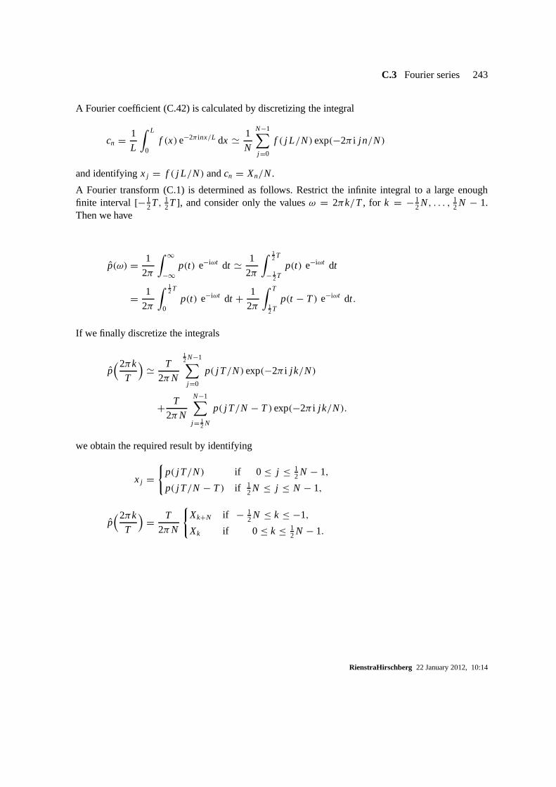
C.3 Fourier series 243
A Fourier coefficient (C.42) is calculated by discretizing the integral
cn = 1
L
∫ L
0f (x)e−2π inx/L dx ' 1
N
N−1∑
j =0
f ( j L/N)exp(−2π i jn/N)
and identifyingx j = f ( j L/N) andcn = Xn/N.
A Fourier transform (C.1) is determined as follows. Restrict the infinite integral to a large enoughfinite interval [−1
2T, 12T], and consider only the valuesω = 2πk/T , for k = −1
2 N, . . . , 12 N − 1.
Then we have
p(ω) = 1
2π
∫ ∞
−∞p(t) e−iωt dt ' 1
2π
∫ 12 T
− 12T
p(t) e−iωt dt
= 1
2π
∫ 12 T
0p(t) e−iωt dt + 1
2π
∫ T
12 T
p(t − T) e−iωt dt.
If we finally discretize the integrals
p(2πk
T
)' T
2πN
12 N−1∑
j =0
p( j T/N)exp(−2π i jk/N)
+ T
2πN
N−1∑
j = 12 N
p( j T/N − T)exp(−2π i jk/N).
we obtain the required result by identifying
x j ={
p( j T/N) if 0 ≤ j ≤ 12 N − 1,
p( j T/N − T) if 12 N ≤ j ≤ N − 1,
p(2πk
T
)= T
2πN
{Xk+N if − 1
2 N ≤ k ≤ −1,
Xk if 0 ≤ k ≤ 12 N − 1.
RienstraHirschberg 22 January 2012, 10:14
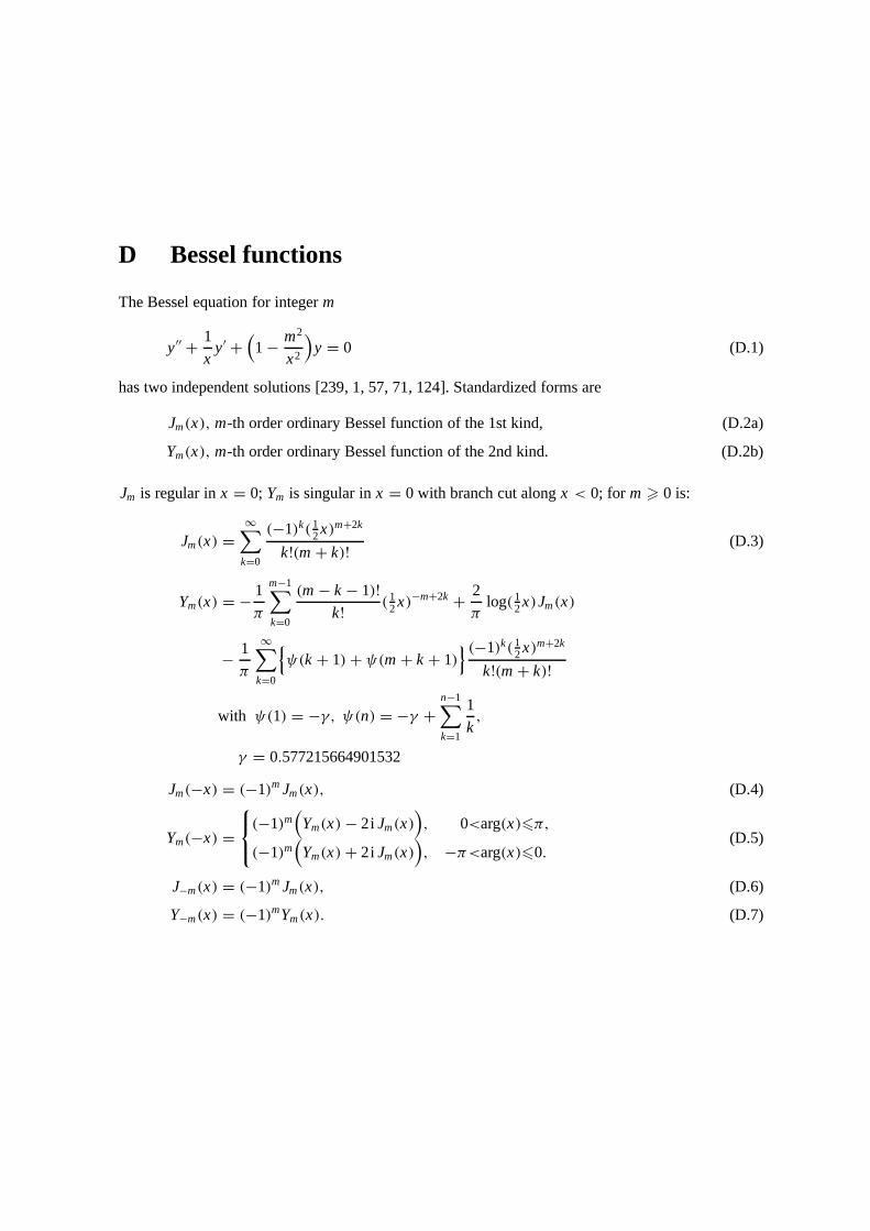
D Bessel functions
The Bessel equation for integerm
y′′ + 1
xy′ +
(1 − m2
x2
)y = 0 (D.1)
has two independent solutions [239, 1, 57, 71, 124]. Standardized forms are
Jm(x), m-th order ordinary Bessel function of the 1st kind, (D.2a)
Ym(x), m-th order ordinary Bessel function of the 2nd kind. (D.2b)
Jm is regular inx = 0; Ym is singular inx = 0 with branch cut alongx < 0; for m > 0 is:
Jm(x) =∞∑
k=0
(−1)k(12x)m+2k
k!(m + k)! (D.3)
Ym(x) = − 1
π
m−1∑
k=0
(m − k − 1)!k! (1
2x)−m+2k + 2
πlog(1
2x)Jm(x)
− 1
π
∞∑
k=0
{ψ(k + 1)+ ψ(m + k + 1)
} (−1)k(12x)m+2k
k!(m + k)!
with ψ(1) = −γ, ψ(n) = −γ +n−1∑
k=1
1
k,
γ = 0.577215664901532
Jm(−x) = (−1)mJm(x), (D.4)
Ym(−x) =
(−1)m
(Ym(x)− 2i Jm(x)
), 0<arg(x)6π,
(−1)m(Ym(x)+ 2i Jm(x)
), −π<arg(x)60.
(D.5)
J−m(x) = (−1)mJm(x), (D.6)
Y−m(x) = (−1)mYm(x). (D.7)
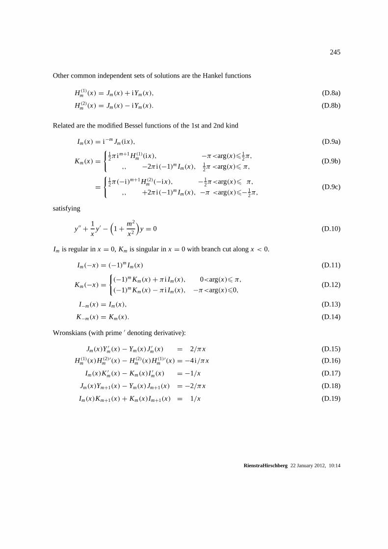
245
Other common independent sets of solutions are the Hankel functions
H (1)m (x) = Jm(x)+ i Ym(x), (D.8a)
H (2)m (x) = Jm(x)− i Ym(x). (D.8b)
Related are the modified Bessel functions of the 1st and 2nd kind
Im(x) = i −mJm(i x), (D.9a)
Km(x) ={
12π i m+1H (1)
m (i x), −π<arg(x)612π,
,, −2π i (−1)mIm(x), 12π <arg(x)6 π,
(D.9b)
={
12π(−i )m+1H (2)
m (−i x), −12π<arg(x)6 π,
,, +2π i (−1)mIm(x), −π <arg(x)6−12π,
(D.9c)
satisfying
y′′ + 1
xy′ −
(1 + m2
x2
)y = 0 (D.10)
Im is regular inx = 0, Km is singular inx = 0 with branch cut alongx < 0.
Im(−x) = (−1)mIm(x) (D.11)
Km(−x) ={(−1)mKm(x)+ π i Im(x), 0<arg(x)6 π,
(−1)mKm(x)− π i Im(x), −π<arg(x)60,(D.12)
I−m(x) = Im(x), (D.13)
K−m(x) = Km(x). (D.14)
Wronskians (with prime′ denoting derivative):
Jm(x)Y′m(x)− Ym(x)J ′
m(x) = 2/πx (D.15)
H (1)m (x)H (2)
m′(x)− H (2)
m (x)H (1)m
′(x) = −4i/πx (D.16)
Im(x)K ′m(x)− Km(x)I ′
m(x) = −1/x (D.17)
Jm(x)Ym+1(x)− Ym(x)Jm+1(x) = −2/πx (D.18)
Im(x)Km+1(x)+ Km(x)Im+1(x) = 1/x (D.19)
RienstraHirschberg 22 January 2012, 10:14
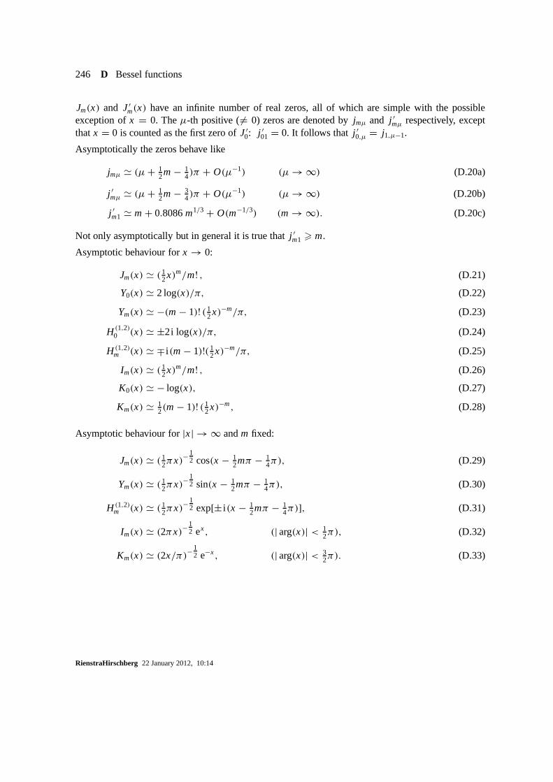
246 D Bessel functions
Jm(x) and J ′m(x) have an infinite number of real zeros, all of which are simple with the possible
exception ofx = 0. Theµ-th positive (6= 0) zeros are denoted byjmµ and j ′mµ respectively, except
thatx = 0 is counted as the first zero ofJ ′0: j ′
01 = 0. It follows that j ′0,µ = j1,µ−1.
Asymptotically the zeros behave like
jmµ ' (µ+ 12m − 1
4)π + O(µ−1) (µ → ∞) (D.20a)
j ′mµ ' (µ+ 1
2m − 34)π + O(µ−1) (µ → ∞) (D.20b)
j ′m1 ' m + 0.8086m1/3 + O(m−1/3) (m → ∞). (D.20c)
Not only asymptotically but in general it is true thatj ′m1 > m.
Asymptotic behaviour forx → 0:
Jm(x) ' (12x)m/m! , (D.21)
Y0(x) ' 2 log(x)/π, (D.22)
Ym(x) ' −(m − 1)! (12x)−m/π, (D.23)
H (1,2)0 (x) ' ±2i log(x)/π, (D.24)
H (1,2)m (x) ' ∓ i (m − 1)!(1
2x)−m/π, (D.25)
Im(x) ' (12x)m/m! , (D.26)
K0(x) ' − log(x), (D.27)
Km(x) ' 12(m − 1)! (1
2x)−m, (D.28)
Asymptotic behaviour for|x| → ∞ andm fixed:
Jm(x) ' (12πx)−
12 cos(x − 1
2mπ − 14π), (D.29)
Ym(x) ' (12πx)−
12 sin(x − 1
2mπ − 14π), (D.30)
H (1,2)m (x) ' (1
2πx)−12 exp[± i (x − 1
2mπ − 14π)], (D.31)
Im(x) ' (2πx)−12 ex, (| arg(x)| < 1
2π), (D.32)
Km(x) ' (2x/π)−12 e−x, (| arg(x)| < 3
2π). (D.33)
RienstraHirschberg 22 January 2012, 10:14
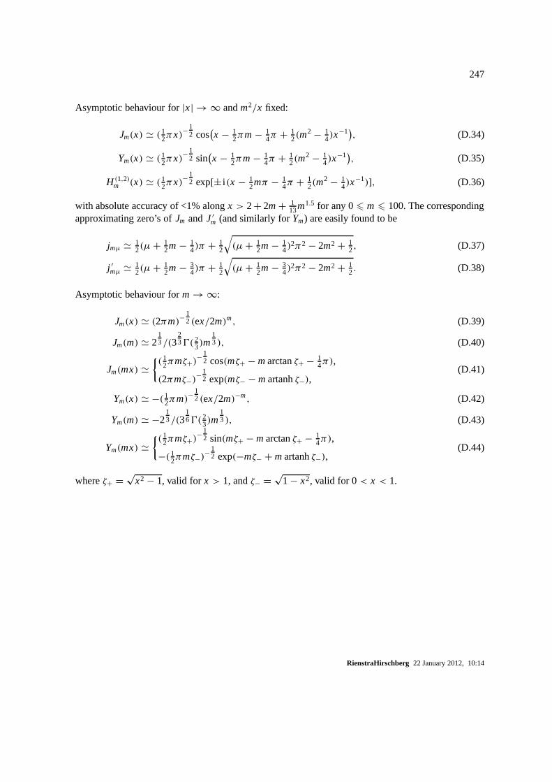
247
Asymptotic behaviour for|x| → ∞ andm2/x fixed:
Jm(x) ' (12πx)−
12 cos
(x − 1
2πm − 14π + 1
2(m2 − 1
4)x−1
), (D.34)
Ym(x) ' (12πx)−
12 sin
(x − 1
2πm − 14π + 1
2(m2 − 1
4)x−1), (D.35)
H (1,2)m (x) ' (1
2πx)−12 exp[± i (x − 1
2mπ − 14π + 1
2(m2 − 1
4)x−1)], (D.36)
with absolute accuracy of <1% alongx > 2+ 2m+ 113m1.5 for any 06 m 6 100. The corresponding
approximating zero’s ofJm andJ ′m (and similarly forYm) are easily found to be
jmµ ' 12(µ+ 1
2m − 14)π + 1
2
√(µ+ 1
2m − 14)
2π2 − 2m2 + 12, (D.37)
j ′mµ ' 1
2(µ+ 12m − 3
4)π + 12
√(µ+ 1
2m − 34)
2π2 − 2m2 + 12. (D.38)
Asymptotic behaviour form → ∞:
Jm(x) ' (2πm)−12 (ex/2m)m, (D.39)
Jm(m) ' 213/(3
230(2
3)m13 ), (D.40)
Jm(mx) '{(1
2πmζ+)− 1
2 cos(mζ+ − marctanζ+ − 14π),
(2πmζ−)− 1
2 exp(mζ− − martanhζ−),(D.41)
Ym(x) ' −(12πm)−
12 (ex/2m)−m, (D.42)
Ym(m) ' −213/(3
160(2
3)m13 ), (D.43)
Ym(mx) '{(1
2πmζ+)− 1
2 sin(mζ+ − marctanζ+ − 14π),
−(12πmζ−)
− 12 exp(−mζ− + martanhζ−),
(D.44)
whereζ+ =√
x2 − 1, valid forx > 1, andζ− =√
1 − x2, valid for 0< x < 1.
RienstraHirschberg 22 January 2012, 10:14

248 D Bessel functions
Important recurrence relations are
Jm−1(x)+ Jm+1(x) = 2mx Jm(x), (D.45)
Jm−1(x)− Jm+1(x) = 2J ′m(x), (D.46)
Ym−1(x)+ Ym+1(x) = 2mx Ym(x), (D.47)
Ym−1(x)− Ym+1(x) = 2Y′m(x), (D.48)
Im−1(x)+ Im+1(x) = 2I ′m(x), (D.49)
Im−1(x)− Im+1(x) = 2mx Im(x), (D.50)
Km−1(x)+ Km+1(x) = −2K ′m(x), (D.51)
Km−1(x)− Km+1(x) = −2mx Km(x). (D.52)
In particular:
J ′0(x) = −J1(x), Y′
0(x) = −Y1(x),
I ′0(x) = I1(x), K ′
0(x) = −K1(x).(D.53)
Some useful relations involving series are
eix cosϑ =∞∑
m=−∞i mJm(x)eimϑ, (D.54)
J0(k R) =∞∑
m=−∞eim(ϑ−ϕ) Jm(kr)Jm(k%), (D.55)
where: R2 = r 2 + %2 − 2r% cos(ϑ − ϕ),
1
r0δ(r − r0) =
∞∑
µ=1
Jm( j ′mµr0)Jm( j ′
mµr )12(1 − m2/ j ′2
mµ)Jm( j ′mµ)
2(0< r, r0 < 1),
∞∑
µ=1
Jm( jmµr0)Jm( jmµr )12 J ′
m( jmµ)2(0< r, r0 < 1).
(D.56)
RienstraHirschberg 22 January 2012, 10:14
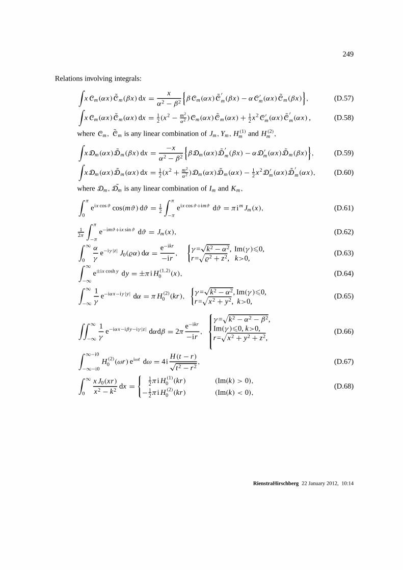
249
Relations involving integrals:∫
xCm(αx)Cm(βx)dx = x
α2 − β2
{βCm(αx)C
′m(βx) − αC ′
m(αx)Cm(βx)}, (D.57)
∫xCm(αx)Cm(αx)dx = 1
2(x2 − m2
α2 )Cm(αx)Cm(αx)+ 12x2C ′
m(αx)C′m(αx) , (D.58)
whereCm, Cm is any linear combination ofJm,Ym, H (1)m andH (2)
m ,
∫xDm(αx)Dm(βx)dx = −x
α2 − β2
{βDm(αx)D
′m(βx) − αD ′
m(αx)Dm(βx)}, (D.59)
∫xDm(αx)Dm(αx)dx = 1
2(x2 + m2
α2 )Dm(αx)Dm(αx)− 12x2D ′
m(αx)D′m(αx), (D.60)
whereDm, Dm is any linear combination ofIm andKm,
∫ π
0eix cosϑ cos(mϑ)dϑ = 1
2
∫ π
−πeix cosϑ+imϑ dϑ = π i mJm(x), (D.61)
12π
∫ π
−πe−imϑ+ix sinϑ dϑ = Jm(x), (D.62)
∫ ∞
0
α
γe−iγ |z| J0(%α)dα = e−ikr
−i r,
{γ=
√k2 − α2, Im(γ )60,
r =√%2 + z2, k>0,
(D.63)
∫ ∞
−∞e±ix coshy dy = ±π i H (1,2)
0 (x), (D.64)
∫ ∞
−∞
1
γe−iαx−iγ |y| dα = πH (2)
0 (kr),
{γ=
√k2 − α2, Im(γ )60,
r =√
x2 + y2, k>0,(D.65)
∫∫ ∞
−∞
1
γe−iαx−iβy−iγ |z| dαdβ = 2π
e−ikr
−i r,
γ=√
k2 − α2 − β2,Im(γ )60, k>0,r =
√x2 + y2 + z2,
(D.66)
∫ ∞−i0
−∞−i0H (2)
0 (ωr )eiωt dω = 4iH (t − r )√
t2 − r 2, (D.67)
∫ ∞
0
x J0(xr)
x2 − k2dx =
{12π i H (1)
0 (kr) (Im(k) > 0),
−12π i H (2)
0 (kr) (Im(k) < 0),(D.68)
RienstraHirschberg 22 January 2012, 10:14

250 D Bessel functions
∫ ∞
0x Jm(αx)Jm(βx)dx = δ(α − β)√
αβ(α, β > 0), (D.69)
∫ ∞
0xYm(αx)Jm(βx)dx = 2
π
1
α2 − β2
(β
α
)m
(Princ. Val.), (D.70)
∫ ∞
0J0(αx) sin(βx)dx = H (β − α)√
β2 − α2, (α, β > 0) (D.71)
∫ ∞
0J0(αx) cos(βx)dx = H (α − β)√
α2 − β2, (α, β > 0) (D.72)
∫ ∞
0Y0(αx) sin(βx)dx =
2
π
1√α2 − β2
arcsin(βα) (0<β<α),
2
π
−1√β2 − α2
arcosh(βα) (0<α<β),
(D.73)
∫ ∞
0Y0(αx) cos(βx)dx = − H (β − α)√
β2 − α2, (α, β > 0) (D.74)
∫ ∞
0K0(αx) sin(βx)dx = 1√
α2 + β2arsinh(β
α), (α, β > 0) (D.75)
∫ ∞
0K0(αx) cos(βx)dx =
12π√α2 + β2
(α, β > 0) (D.76)
Related to Bessel functions of order13 are the Airy functionsAi andBi [1], given by
Ai(x) = 1
π
∫ ∞
0cos(1
3t3 + xt)dt (D.77)
Bi(x) = 1
π
∫ ∞
0
[exp(−1
3t3 + xt)+ sin(13t3 + xt)
]dt (D.78)
They are solutions of
y′′ − xy = 0, (D.79)
RienstraHirschberg 22 January 2012, 10:14

251
with the following asymptotic behaviour (introduceζ = 23|x|3/2)
Ai(x) '
cos(ζ − 14π)√
π |x|1/4 (x → −∞),
e−ζ
2√π x1/4
(x → ∞),
(D.80)
Bi(x) '
cos(ζ + 14π)√
π |x|1/4 (x → −∞),
eζ√π x1/4
(x → ∞).
(D.81)
0
0.5
1
2 4 6 8 10 12 14
Figure D.1 Bessel functionJn(x) as function of order and argument.
RienstraHirschberg 22 January 2012, 10:14
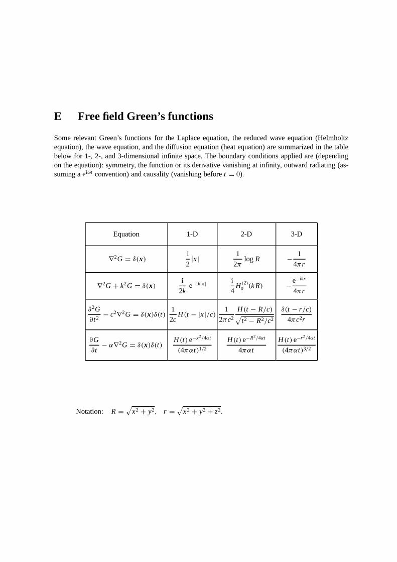
E Free field Green’s functions
Some relevant Green’s functions for the Laplace equation, the reduced wave equation (Helmholtzequation), the wave equation, and the diffusion equation (heat equation) are summarized in the tablebelow for 1-, 2-, and 3-dimensional infinite space. The boundary conditions applied are (dependingon the equation): symmetry, the function or its derivative vanishing at infinity, outward radiating (as-suming aeiωt convention) and causality (vanishing beforet = 0).
Equation 1-D 2-D 3-D
∇2G = δ(x)1
2|x| 1
2πlog R − 1
4πr
∇2G + k2G = δ(x)i
2ke−ik|x| i
4H (2)
0 (k R) −e−ikr
4πr
∂2G
∂t2− c2∇2G = δ(x)δ(t)
1
2cH (t − |x|/c) 1
2πc2
H (t − R/c)√t2 − R2/c2
δ(t − r/c)
4πc2r
∂G
∂t− α∇2G = δ(x)δ(t)
H (t)e−x2/4αt
(4παt)1/2H (t)e−R2/4αt
4παt
H (t)e−r 2/4αt
(4παt)3/2
Notation: R =√
x2 + y2, r =√
x2 + y2 + z2.
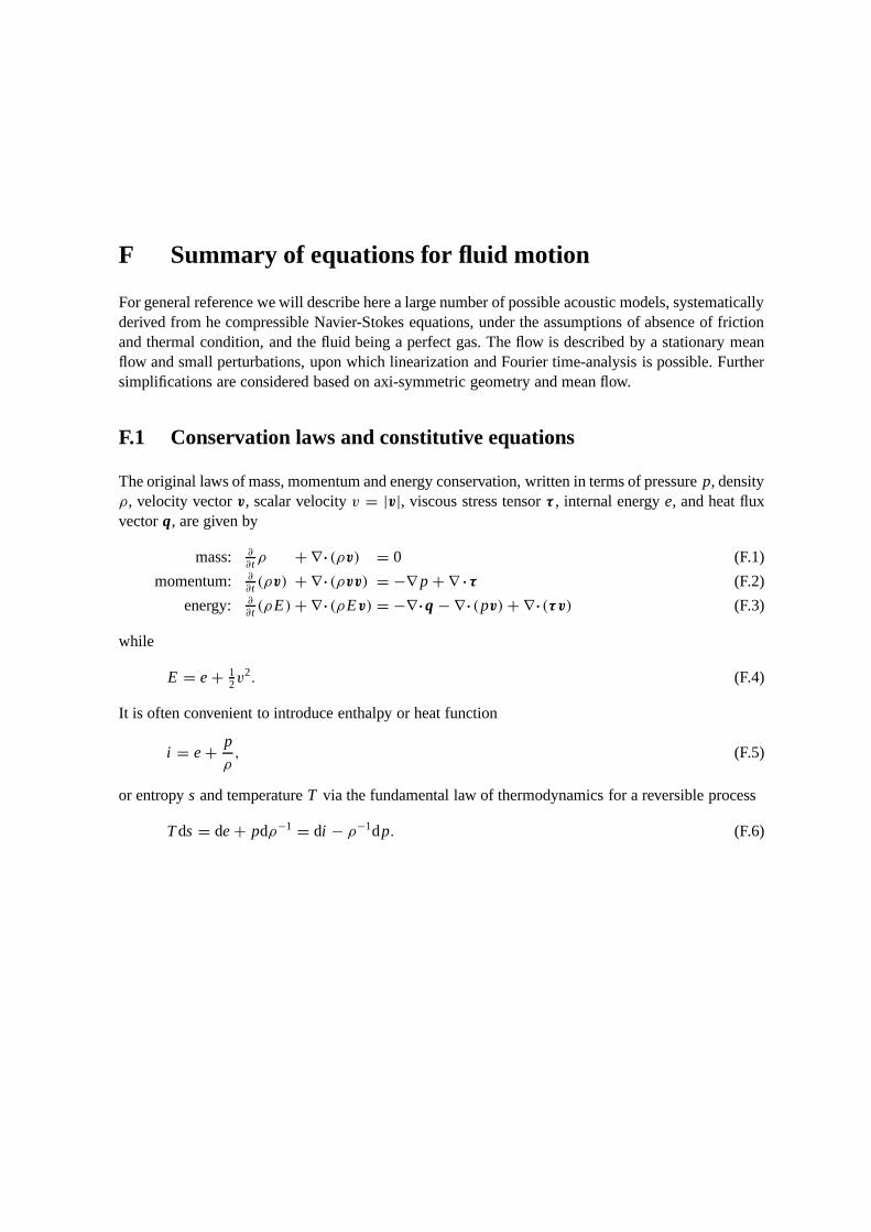
F Summary of equations for fluid motion
For general reference we will describe here a large number ofpossible acoustic models, systematicallyderived from he compressible Navier-Stokes equations, under the assumptions of absence of frictionand thermal condition, and the fluid being a perfect gas. The flow is described by a stationary meanflow and small perturbations, upon which linearization and Fourier time-analysis is possible. Furthersimplifications are considered based on axi-symmetric geometry and mean flow.
F.1 Conservation laws and constitutive equations
The original laws of mass, momentum and energy conservation, written in terms of pressurep, densityρ, velocity vectorv, scalar velocityv = |v|, viscous stress tensorτ , internal energye, and heat fluxvectorq, are given by
mass: ∂∂t ρ + ∇·(ρv) = 0 (F.1)
momentum: ∂∂t (ρv) + ∇·(ρvv) = −∇ p + ∇ ·τ (F.2)
energy: ∂∂t (ρE)+ ∇·(ρEv) = −∇·q − ∇·(pv)+ ∇·(τv) (F.3)
while
E = e+ 12v
2. (F.4)
It is often convenient to introduce enthalpy or heat function
i = e+ p
ρ, (F.5)
or entropys and temperatureT via the fundamental law of thermodynamics for a reversible process
Tds = de+ pdρ−1 = di − ρ−1dp. (F.6)
254 F Summary of equations for fluid motion
With ddt = ∂
∂t + v ·∇ for the convective derivative, the above conservation lawsmay be reduced to
mass: ddtρ = −ρ∇·v (F.7a)
momentum: ρ ddt v = −∇ p + ∇ ·τ (F.7b)
energy : ρ ddt e = −∇·q − p∇·v + τ :∇v (F.7c)
ρ ddt i = d
dt p − ∇·q + τ :∇v (F.7d)
ρT ddt s = −∇·q + τ :∇v. (F.7e)
For acoustic applications the entropy form (F.7e) is the most convenient.
For anideal gas we have the following relations
p = ρRT, de = CVdT, di = CPdT (F.8a,b,c)
whereCV is the heat capacity or specific heat at constant volume,CP is the heat capacity or specificheat at constant pressure [112].CV = CV(T) andCP = CP(T) are in general functions of temper-ature.R is the specific gas constant andγ the specific-heat ratio, which are practically constant andgiven by (the figures refer to air)
R = CP − CV = 286.73 J/kg K, γ = CP
CV= 1.402 (F.9a,b)
From equation (F.6) it then follows for an ideal gas that
ds = CVdp
p− CP
dρ
ρ(F.10)
while isentropic perturbations (ds = 0), like sound, propagate with the sound speedc given by
c2 =(∂p
∂ρ
)s= γ p
ρ= γ RT. (F.11)
For aperfectgas, the specific heats are constant (independent ofT ), and we can integrate
e = CV T + einit, i = CPT + i init, s = CV log p − CP logρ + sinit. (F.12a,b,c)
The integration “constants”einit, i init andsinit refer to the initial situation of each particle. So this resultis only useful if we start with a fluid of uniform thermodynamical properties, or if we are able to traceback the pathlines (or streamlines for a steady flow).
RienstraHirschberg 22 January 2012, 10:14
F.2 Acoustic approximation 255
F.2 Acoustic approximation
F.2.1 Inviscid and isentropic
In the acoustic realm we will consider, the viscous or turbulent stress terms will be assumed to play arole only in an aerodynamic source region, while any perturbation is too fast to be affected by thermalconduction. Therefore, for the applications of acoustic propagation we will ignore viscous shear stress(τ ) and thermal conduction (q). In particular, this is obtained as follows. We make dimensionless byscaling
x := Lx, v := v0v, t := L
v0t, ρ := ρ0ρ,
dp := ρ0v20dp, τ := µv0
Lτ , q := κ1T
Lq,
T := T0T, dT := 1TdT, ds := CP1T
T0ds
to get
ddt ρ = −ρ∇·v (F.13a)
ρ ddt v = −∇ p + 1
Re∇ ·τ (F.13b)
ρT ddt s = − 1
Pe∇·q + Ec
Reτ :∇v, (F.13c)
whereRe = ρ0v0L/µ denotes the Reynolds number,Pe = ρ0CPv0L/κ the Peclet number, andEc = v2
0/CP1T the Eckert number. If the Reynolds number tends to infinity, usually also the Pecletnumber does, becausePe = PrRe and the Prandtl numberPr is for most fluids and gases of order 1.Then, provided the Eckert number is not large, we obtain
ddtρ = −ρ∇·v (F.14a)
ρ ddt v = −∇ p (F.14b)ddt s = 0 (F.14c)
which means that entropy remains constant, and thus dh = ρ−1dp, along streamlines.
Furthermore, we will assume the gas to be perfect, with the following thermodynamical closure rela-tions
ds = CVdp
p− CP
dρ
ρ, c2 = γ p
ρ. (F.14d)
RienstraHirschberg 22 January 2012, 10:14
256 F Summary of equations for fluid motion
By substituting equation (F.14d) into equation (F.14c) we obtain
ddt p = c2 d
dt ρ. (F.14e)
If the flow is initially homentropic (sinit is uniformly constant) then
p ∝ ργ es/CV (F.14f)
If the flow is homentropic (s is uniformly constant) then
p ∝ ργ (F.14g)
F.2.2 Perturbations of a mean flow
When we have a stationary mean flow with instationary perturbations, given by
v = v0 + v′, p = p0 + p′, ρ = ρ0 + ρ ′, s = s0 + s′ (F.15)
and linearize for small amplitude, we obtain for the mean flow
∇·(ρ0v0) = 0 (F.16a)
ρ0(v0·∇)v0 = −∇ p0 (F.16b)
(v0·∇)s0 = 0 (F.16c)
while
ds0 = CVdp0
p0− CP
dρ0
ρ0, c2
0 = γ p0
ρ0(F.16d)
and the perturbations
∂∂t ρ
′ + ∇·(v0ρ′ + v′ρ0) = 0 (F.17a)
ρ0(∂∂t + v0·∇)
v′ + ρ0(v′ ·∇)
v0 + ρ ′(v0·∇)v0 = −∇ p′ (F.17b)
( ∂∂t + v0·∇)s′ + v′ ·∇s0 = 0 (F.17c)
while, assumings′init = 0,
s′ = CV
p0p′ − CP
ρ0ρ ′ = CV
p0
(p′ − c2
0ρ′), c′ = 1
2c0
( p′
p0− ρ ′
ρ0
). (F.17d)
The expression forc′ usually serves no purpose.
RienstraHirschberg 22 January 2012, 10:14
F.2 Acoustic approximation 257
From equation (F.14e) we get for the mean flowv0·∇ p0 = c20v0·∇ρ0, and for the perturbations an
equation, equivalent to (F.17c) and (F.17d),
∂∂t p′ + v0·∇ p′ + v′ ·∇ p0 = c2
0
(∂∂t ρ
′ + v0·∇ρ ′ + v′ ·∇ρ0
)+ c2
0
(v0·∇ρ0
)( p′
p0− ρ′
ρ0
). (F.18)
If the mean flow is homentropic (s0 = constant), we have∇ p0 = c20∇ρ0 while the perturbations are
isentropic along streamlines.
If the perturbations are entirely isentropic (s′ ≡ 0), for example whenv0 = 0 ands0 = constant orwhen the flow is homentropic (satisfying equation F.14g), the pressure and density perturbations arerelated by the usual
p′ = c20ρ
′. (F.19)
F.2.3 Myers’ Energy Corollary
Myers’ definition of energy [150, 151, 152] for unsteady disturbances propagating in moving fluidmedia is both consistent with the general conservation law of fluid energy and with the order of ap-proximation in the linear model adopted to describe the disturbances. When the mass and momentumequations (F.1,F.2) and the general energy conservation law (F.3) for fluid motion is expanded toquadratic order, this 2nd order energy term may be reduced tothe following conservation law forperturbation energy densityE, energy fluxI , and dissipationD
∂∂t E + ∇· I = −D (F.20)
where (for simplicity we neglect viscous stress and heat conduction)
E = p′2
2ρ0c20
+ 12ρ0v
′2 + ρ ′v0·v′ + ρ0T0s′2
2Cp, (F.21a)
I =(ρ0v
′ + ρ ′v0)( p′
ρ0+ v0·v′
)+ ρ0v0T ′s′, (F.21b)
D = −ρ0v0·(ω′×v′) − ρ ′v′ ·(ω0×v0)+ s′(ρ0v
′ + ρ ′v0)·∇T0 − s′ρ0v0·∇T ′. (F.21c)
while the vorticity vector is denoted by∇×v = ω = ω0+ω′. Without mean flow this definition reducesto the traditional one. Note that, according to this definition, acoustic energy is entirely conserved inhomentropic, irrotational flow. In vortical flow, the interaction with the mean flow may constitute asource or a sink of acoustic energy.
RienstraHirschberg 22 January 2012, 10:14

258 F Summary of equations for fluid motion
F.2.4 Zero mean flow
Without mean flow, such thatv0 = ∇ p0 = 0, the equations may be reduced to
∂2
∂t2 p′ − ∇·(c20∇ p′) = 0. (F.22)
F.2.5 Time harmonic
When the perturbations are time-harmonic, given by
v′ = Re(v eiωt), p′ = Re( p eiωt), ρ ′ = Re(ρ eiωt), s′ = Re(seiωt), (F.23)
we have in the usual complex notation
iωρ + ∇·(v0ρ + vρ0)
= 0 (F.24a)
ρ0(iω + v0·∇)
v + ρ0(v ·∇)
v0 + ρ(v0·∇)
v0 = −∇ p (F.24b)(iω + v0·∇)
s + v ·∇s0 = 0 (F.24c)
s = Cv
p0
(p − c2
0ρ). (F.24d)
F.2.6 Irrotational isentropic flow
When the flow is irrotational and isentropic everywhere (homentropic), we can introduce a potentialfor the velocity, wherev = ∇φ, and expressp as a function ofρ only, such that we can integrate themomentum equation, and obtain the important simplification
∂
∂tφ + 1
2v2 + c2
γ − 1= constant,
p
ργ= constant. (F.25)
For mean flow with harmonic perturbation, whereφ = φ0 + Re(φ eiωt), we have then for the meanflow
12v
20 + c2
0
γ − 1= constant,
∇·(ρ0v0) = 0,p0
ργ
0
= constant(F.26a)
and for the acoustic perturbations(iω + v0·∇)
ρ + ρ∇·v0 + ∇·(ρ0∇φ)
= 0,
ρ0(iω + v0·∇)
φ + p = 0, p = c20ρ.
(F.26b)
RienstraHirschberg 22 January 2012, 10:14
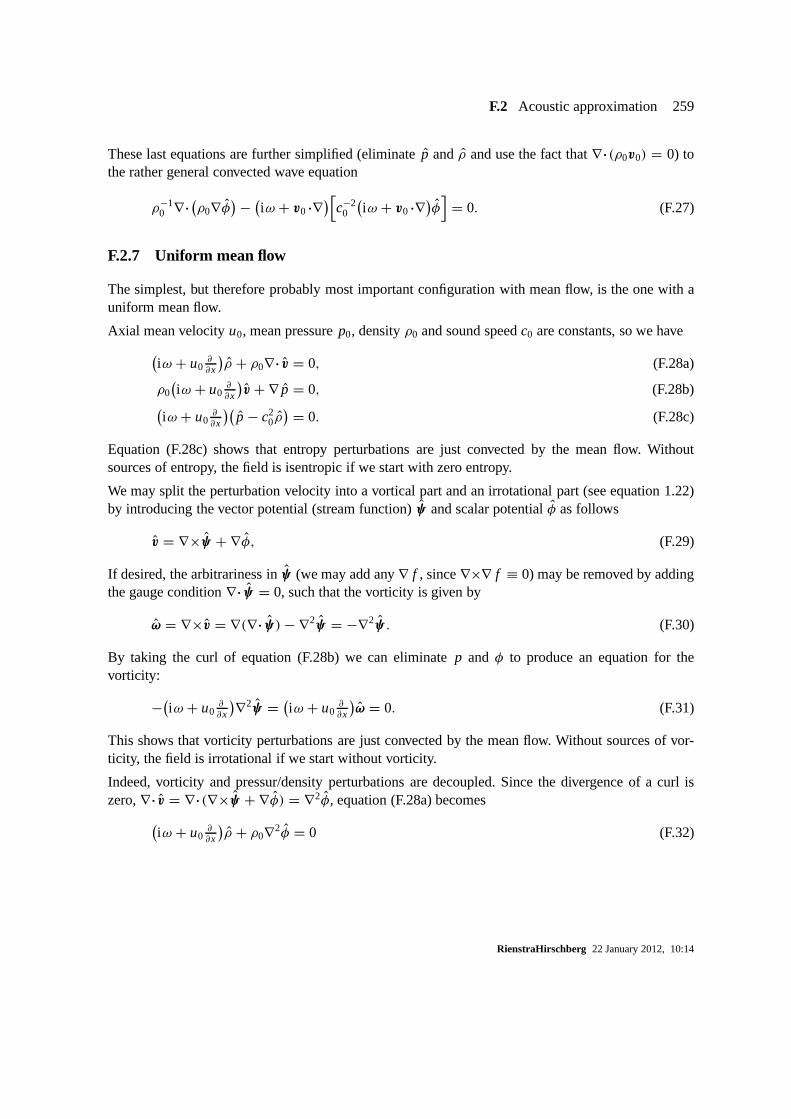
F.2 Acoustic approximation 259
These last equations are further simplified (eliminatep andρ and use the fact that∇·(ρ0v0) = 0) tothe rather general convected wave equation
ρ−10 ∇·(ρ0∇φ
)−
(iω + v0·∇)[
c−20
(iω + v0·∇)
φ]
= 0. (F.27)
F.2.7 Uniform mean flow
The simplest, but therefore probably most important configuration with mean flow, is the one with auniform mean flow.
Axial mean velocityu0, mean pressurep0, densityρ0 and sound speedc0 are constants, so we have
(iω + u0
∂∂x
)ρ + ρ0∇· v = 0, (F.28a)
ρ0(iω + u0
∂∂x
)v + ∇ p = 0, (F.28b)
(iω + u0
∂∂x
)(p − c2
0ρ)
= 0. (F.28c)
Equation (F.28c) shows that entropy perturbations are justconvected by the mean flow. Withoutsources of entropy, the field is isentropic if we start with zero entropy.
We may split the perturbation velocity into a vortical part and an irrotational part (see equation 1.22)by introducing the vector potential (stream function)ψ and scalar potentialφ as follows
v = ∇×ψ + ∇φ, (F.29)
If desired, the arbitrariness inψ (we may add any∇ f , since∇×∇ f ≡ 0) may be removed by addingthe gauge condition∇·ψ = 0, such that the vorticity is given by
ω = ∇×v = ∇(∇·ψ)− ∇2ψ = −∇2ψ . (F.30)
By taking the curl of equation (F.28b) we can eliminatep and φ to produce an equation for thevorticity:
−(iω + u0
∂∂x
)∇2ψ =
(iω + u0
∂∂x
)ω = 0. (F.31)
This shows that vorticity perturbations are just convectedby the mean flow. Without sources of vor-ticity, the field is irrotational if we start without vorticity.
Indeed, vorticity and pressur/density perturbations are decoupled. Since the divergence of a curl iszero,∇· v = ∇·(∇×ψ + ∇φ) = ∇2φ, equation (F.28a) becomes
(iω + u0
∂∂x
)ρ + ρ0∇2φ = 0 (F.32)
RienstraHirschberg 22 January 2012, 10:14

260 F Summary of equations for fluid motion
By taking the divergence of equation (F.28b), and using equations (F.28a,F.28c), not assuming isen-tropy or irrotationality, we can eliminateφ andρ to obtain the convected reduced wave equation forthe pressure
c20∇2 p −
(iω + u0
∂∂x
)2p = 0. (F.33)
Plane wave solutions are given by
p = Ae−ik·x, v = kρ0�
Ae−ik·x, � = ω − u0kx, c20|k|2 = �2, (F.34)
not propagating ink-direction but in the direction of the intensity vector
〈I〉 = ω|A|22ρ0�2
(k + M0|k|ex
), M0 = u0/c0. (F.35)
With some care, especially taking due notice of any singularedge behaviour, equation (F.33) may betransformed to the ordinary reduced wave equation
c20∇2 p +�2 p = 0 (F.36)
by introducing
p(x, r, θ;ω) = p(X, r, θ;�)exp(i �Mc0
X), (F.37)
where x = βX, ω = β�, M = u0
c0, β =
√1 − M2.
RienstraHirschberg 22 January 2012, 10:14
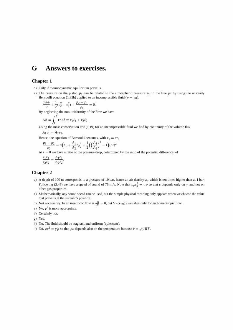
G Answers to exercises.
Chapter 1d) Only if thermodynamic equilibrium prevails.
e) The pressure on the pistonp1 can be related to the atmospheric pressurep2 in the free jet by using the unsteadyBernoulli equation (1.32b) applied to an incompressible fluid (ρ = ρ0):∂1φ
∂t+ 1
2(v2
2 − v21)+ p2 − p1
ρ0= 0.
By neglecting the non-uniformity of the flow we have
1φ =∫ 2
1v·d` ' v1`1 + v2`2.
Using the mass conservation law (1.19) for an incompressible fluid we find by continuity of the volume flux
A1v1 = A2v2.
Hence, the equation of Bernoulli becomes, withv1 = at,p1 − p2
ρ0= a
(`1 + A1
A2`2
)+ 1
2
(( A1
A2
)2− 1
)(at)2.
At t = 0 we have a ratio of the pressure drop, determined by the ratioof the potential difference, ofv1`1
v2`2= A1`1
A2`2.
Chapter 2a) A depth of 100 m corresponds to a pressure of 10 bar, hence anair densityρg which is ten times higher than at 1 bar.
Following (2.45) we have a speed of sound of 75 m/s. Note thatρgc2g = γ p so thatc depends only onγ and not on
other gas properties.
c) Mathematically, any sound speed can be used, but the simple physical meaning only appears when we choose the valuethat prevails at the listener’s position.
d) Not necessarily. In an isentropic flow isDsDt = 0, but∇·(vρ0)) vanishes only for an homentropic flow.
e) No, p′ is more appropriate.
f) Certainly not.
g) Yes.
h) No. The fluid should be stagnant and uniform (quiescent).
i) No. ρc2 = γ p so thatρc depends also on the temperature becausec =√γ RT.

262 G Answers to exercises.
Chapter 3a) Every point of the line source has a different distance, and therefore different travel time, to the observer. Note thetail
of the 2-D wave-equation Green’s function (Appendix E)(2πc2)−1H(t − R/c)/√
t2 − R2/c2.
b) The fieldP of one point source is given by (see Appendix E)Pt t − c2∇2P = δ(t − τ)δ(x − x0)δ(y − y0)δ(z) with solutionP = δ(t − τ − r0/c)/4πc2r0 wherer0 = {(x − x0)
2 + (y − y0)2 + z2}1/2.
Integrate over allx0, y0, introducex0 = x + {r 20 − z2}1/2 cosθ0 and
y0 = y + {r 20 − z2}1/2 sinθ0, and obtain the total field
p =∫∫
P dx0dy0 = 2π4πc2
∫ ∞|z| δ(t − τ − r0/c) dr0 = (2c)−1H(t − τ − |z|/c).
This could have been anticipated from the fact that the problem is really one dimensional.
c) From Appendix E we find the total field
p(x, y, z) = 14 i
∞∑
n=−∞H (2)
0 (k Rn) ' 14 i
∞∑
n=−∞(1
2πk Rn)− 1
2 exp(14π i − i k Rn)
whereRn = ((x − nd)2 + y2)12 = (r 2 − 2rnd cosθ + n2d2)
12 .
Consider the sources satisfying−r � nd � r , such that
Rn ' r − ndcosθ (r → ∞).
This part of the series looks like
· · · ' 14 i
∑(1
2πkr)−12 exp(1
4π i − i kr + i kndcosθ)
and grows linearly with the number of terms ifexp(i kndcosθ) = 1, orkdcosθ = 2πm.
d) The condition is now exp(−iπn + i kndcosθ) = 1, orkdcosθ = (2m + 1).
e) If we makex dimensionless by a length scaleL , we haveδ(x) = δ( xL L) = 1
L δ(xL ). So the dimension ofδ(x) is
(length)−1.
f) Multiply by a test functionφ(x, y) and integrate
· · · = −∫∫
1
rφr dx dy = −
∫ 2π
0
∫ ∞
0φr dr dθ = 2πφ(0, 0).
g) Let Sbe given by an equationf (x) = 0, such thatf (x) > 0 if and only if x ∈ V . The outward normaln is then givenby n = −(∇ f/|∇ f |) f =0. SinceH( f )v vanishes outsideV , we have
0 =∫
∇·[H( f )v]dx =
∫ [H( f )∇·v + δ( f ) v·∇ f
]dx
=∫
V∇·v dx −
∫
Sv·n dσ.
h) Only the terms contribute which satisfy 0< 2nL ≤ c0t , so we obtain
(2 + R)g(t) = R f(t)+ 2bc0t/2Lc∑
n=1
(f(t − 2nL
c0
)− g
(t − 2nL
c0
)).
i) p(x) = e−ikx +Reikx. If p(x0) = 0, we haveR = − e−2ikx0.Since p(x0) = 0 andv(x0) 6= 0 we have simplyZ = 0.
j) v(x) = (ρ0c0)−1(e−ikx −Reikx). If v(x0) = 0, we haveR = e−2ikx0.
Sincev(x0) = 0 and p(x0) 6= 0 we have simplyZ = ∞.
RienstraHirschberg 22 January 2012, 10:14
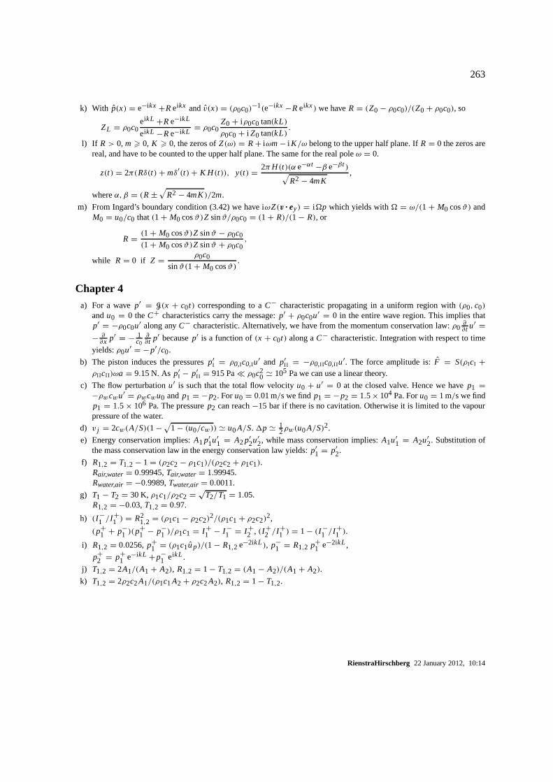
263
k) With p(x) = e−ikx +Reikx andv(x) = (ρ0c0)−1(e−ikx −Reikx) we haveR = (Z0 − ρ0c0)/(Z0 + ρ0c0), so
ZL = ρ0c0eikL +Re−ikL
eikL −Re−ikL= ρ0c0
Z0 + iρ0c0 tan(kL)
ρ0c0 + i Z0 tan(kL).
l) If R> 0, m > 0, K > 0, the zeros ofZ(ω) = R+ iωm− i K/ω belong to the upper half plane. IfR = 0 the zeros arereal, and have to be counted to the upper half plane. The same for the real poleω = 0.
z(t) = 2π(Rδ(t)+ mδ′(t)+ K H(t)), y(t) = 2πH(t)(α e−αt −β e−βt )√R2 − 4mK
,
whereα, β = (R ±√
R2 − 4mK)/2m.
m) From Ingard’s boundary condition (3.42) we have iωZ(v·ey) = i�p which yields with� = ω/(1 + M0 cosϑ) andM0 = u0/c0 that(1 + M0 cosϑ)Z sinϑ/ρ0c0 = (1 + R)/(1 − R), or
R = (1 + M0 cosϑ)Z sinϑ − ρ0c0
(1 + M0 cosϑ)Z sinϑ + ρ0c0,
while R = 0 if Z = ρ0c0
sinϑ(1 + M0 cosϑ).
Chapter 4a) For a wavep′ = G(x + c0t) corresponding to aC− characteristic propagating in a uniform region with(ρ0, c0)
andu0 = 0 theC+ characteristics carry the message:p′ + ρ0c0u′ = 0 in the entire wave region. This implies thatp′ = −ρ0c0u′ along anyC− characteristic. Alternatively, we have from the momentum conservation law:ρ0
∂∂t u′ =
− ∂∂x p′ = − 1
c0∂∂t p′ becausep′ is a function of(x + c0t) along aC− characteristic. Integration with respect to time
yields:ρ0u′ = −p′/c0.
b) The piston induces the pressuresp′I = ρ0,Ic0,Iu
′ and p′II = −ρ0,II c0,II u
′. The force amplitude is:F = S(ρIcI +ρII cII )ωa = 9.15 N. As p′
I − p′II = 915 Pa� ρ0c2
0 ' 105 Pa we can use a linear theory.
c) The flow perturbationu′ is such that the total flow velocityu0 + u′ = 0 at the closed valve. Hence we havep1 =−ρwcwu′ = ρwcwu0 and p1 = −p2. Foru0 = 0.01 m/s we findp1 = −p2 = 1.5× 10⁴ Pa. Foru0 = 1 m/s we findp1 = 1.5 × 10⁶ Pa. The pressurep2 can reach−15 bar if there is no cavitation. Otherwise it is limited to the vapourpressure of the water.
d) v j = 2cw(A/S)(1 −√
1 − (u0/cw)) ' u0A/S.1p ' 12ρw(u0A/S)2.
e) Energy conservation implies:A1p′1u′
1 = A2p′2u′
2, while mass conservation implies:A1u′1 = A2u′
2. Substitution ofthe mass conservation law in the energy conservation law yields: p′
1 = p′2.
f) R1,2 = T1,2 − 1 = (ρ2c2 − ρ1c1)/(ρ2c2 + ρ1c1).Rair,water = 0.99945,Tair,water = 1.99945.Rwater,air = −0.9989,Twater,air = 0.0011.
g) T1 − T2 = 30 K,ρ1c1/ρ2c2 =√
T2/T1 = 1.05.R1,2 = −0.03, T1,2 = 0.97.
h) (I −1 /I +
1 ) = R21,2 = (ρ1c1 − ρ2c2)
2/(ρ1c1 + ρ2c2)2,
(p+1 + p−
1 )(p+1 − p−
1 )/ρ1c1 = I +1 − I −
1 = I +2 , (I +
2 /I +1 ) = 1 − (I −
1 /I +1 ).
i) R1,2 = 0.0256,p+1 = (ρ1c1up)/(1 − R1,2 e−2ikL), p−
1 = R1,2 p+1 e−2ikL,
p+2 = p+
1 e−ikL +p−1 eikL.
j) T1,2 = 2A1/(A1 + A2), R1,2 = 1 − T1,2 = (A1 − A2)/(A1 + A2).
k) T1,2 = 2ρ2c2A1/(ρ1c1A2 + ρ2c2A2), R1,2 = 1 − T1,2.
RienstraHirschberg 22 January 2012, 10:14

264 G Answers to exercises.
l) limA2/A1→0
R1,2 = 1, limA2/A1→∞
R1,2 = −1.
m) For an orifice with wall thicknessL and cross-sectional areaAd in a pipe of cross-sectional areaAp we have:R =p−
1 /p+1 =
i k(L + 2δ)Ap/[2Ad + i k(L + 2δ)Ap], wherek = ω/c0, δ ' 83π
√Ad/π .
p) Without mean flow (u0 = 0):
• At low amplitudes, when linear theory is valid, friction is negligible whenδ2v = 2ν/ω � Ad.
• At large amplitudes,u2/ω2Ad > 1, flow separation will occur. Flow separation is induced by viscosity. Ifδ2v � Adthen the exact value of the viscosity is not important to predict flow separation. We have reached a high Reynoldsnumber limit.
With mean flow (u0 6= 0), we have the same answer as for large amplitudes.
o) Flow separation always occurs when the particle displacement is of the order of the diameter of the orifice:u′d ∼ ωd.
In the pipe we have:u′D = u′
d(d/D)2. The critical level is given byp′ ∼ ρ0c0ωd(d/D)2.At 10 Hz this corresponds to SPL = 110 dB.At 100 Hz this corresponds to SPL = 130 dB.At 1000 Hz this corresponds to SPL = 150 dB.Within a hearing-aid device, sound is transferred from the amplifier (at the back of the ear) to the ear-drum by meansof a pipe ofD = 1 mm. An orifice ofd = 0.1 mm placed in this pipe, will protect the ear by limiting sound levelaround 1 kHz to SPL = 130 dB. Such devices are indeed in everyday use.
p) In a stationary subsonic free jet induced by a mean flow we expect a uniform pressure. The first intuitive guess for aquasi-stationary theory is to assume that the inertial effects upstream of the orifice remain unchanged, while the inertialeffects in the jet are negligible. This leads to the common assumption that the end correction of a thin orifice witha mean flow is at low frequencies half of the end correction in the absence of mean flow. Experiments by Ajello [2]indicate a much stronger reduction of the end-correction. In some circumstances negative end corrections are found (Ajello [2], Peters [171]). Indeed the theory for open pipe termination of Rienstra [187] indicates that we cannot predictend corrections intuitively.
q) R = p−1 /p+
1 = [A1 − (A2 + A3)]/[A1 + (A2 + A3)].r) R = p−
1 /p+1 = [(A1 − A3) cos(kL)− i A2 sin(kL)]/[(A1 − A3) cos(kL)+ i A2 sin(kL)].
R = −1 for kL = π(n + 0.5), R = 0 for A2 = 0 when A1 = A3 and R = 1 for A3 = 0 whenkL = nπ(n = 0,1, 2,3, . . . ).
s) p+1 + p−
1 = pb + ρwω2a0a. pb/p0 = −3γ a/a0. p−
1 = Rp+1 .
A( p+1 − p−
1 ) = Ap+2 − (ρwcw)iω4πa2
0a. p+1 + p−
1 = p+2 .
R = −[1 + i A(ω2 − ω20)/2πωcwa0]−1 with ω2
0 = 3γ p0/ρwa20.
t) pb/ pin = [1 + ( ωω0)2(2π ia0
Ak − 1)]−1.
u) ω20a2
0/c2l = 3ρl /ρw � 1. At p0 = 1 bar,ρl /ρw = O(10−3).
v) 3γl p0/ρwc2w = O(10−4) hencea0ω/cw < 10−2.
w) ω20 ' 3γl p0/2ρwa2
0. R = −[1 + A(ω2 − ω20)/2π iωcwa0]−1.
x) Whena0 = O(D) we do not have a radial flow around the bubble. The approximation used for small bubbles fails.
y) [g] = s/m.
z) ω2g − c20
d2
dx2 g = e−iωτ δ(x − y)/2π .
Integration aroundx = y yields:−[ ddx g]y+
y− = e−iωτ /2πc20.
[ ddx g]± = ∓i kg±. At x = y we haveg± = e−iωτ /4π iωc0.
RienstraHirschberg 22 January 2012, 10:14
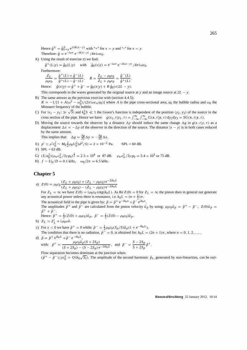
265
Henceg± = g±x=y e∓ik(x−y) with “+” for x > y and “-” for x < y.
Therefore:g = e−iωτ e−ik|x−y| /4π iωc0.
A) Using the result of exercise z) we find:
g+(L |y) = g0(L |y) with g0(x|y) = e−iωτ e−ik|x−y| /4π iωc0.
Furthermore:ZL
ρ0c0= g+(L)+ g−(L)
g+(L)− g−(L), R = ZL − ρ0c0
ZL + ρ0c0= g−(L)
g+(L).
Hence: g(x|y) = g+ + g− = g0(x|y) + Rg0(x|2L − y).
This corresponds to the waves generated by the original source aty and an image source at 2L − y.
B) The same answer as the previous exercise with (section 4.4.5):R = −1/[1 + A(ω2 − ω2
0)/(2π iωcwa0)] whereA is the pipe cross-sectional area,a0 the bubble radius andω0 theMinnaert frequency of the bubble.
C) For |x1 − y1| �√
S| andk20S � 1 the Green’s function is independent of the position(y2, y3) of the source in the
cross section of the pipe. Hence we have:g(x1, t |y1, τ ) =∫ ∞−∞
∫ ∞−∞ G(x, t |y, τ ) dy2dy3 = SG(x, t |y, τ ).
D) Moving the source towards the observer by a distance1y should induce the same change1g in g(x, t |y, τ ) as adisplacement1x = −1y of the observer in the direction of the source. The distance|x − y| is in both cases reducedby the same amount.This implies that: 1g = ∂g
∂y1y = − ∂g∂x1x.
E) p′ ' ρ′c20 ∼ M0
12ρ0U2
0 (d2/S) = 2 × 10⁻² Pa. SPL = 60 dB.
F) SPL = 63 dB.
G) (S/a20)(ρwc2
w/3γ p0)12 = 2.3 × 10⁴ or 87 dB. ρwc2
w/3γ p0 = 5.4 × 10³ or 75 dB.
H) f ∼ U0/D = 0.1 kHz, ω0/2π = 6.5 kHz.
Chapter 5
a) Z(0) = ρ0c0(ZL + ρ0c0)+ (ZL − ρ0c0) e−2ik0L
(ZL + ρ0c0)− (ZL − ρ0c0) e−2ik0L
For ZL = ∞ we haveZ(0) = iρ0c0 cotg(k0L). As ReZ(0) = 0 for ZL = ∞ the piston does in general not generateany acoustical power unless there is resonance,i.e. k0L = (n + 1
2)π .
The acoustical field in the pipe is given by:p = p+ e−ik0x + p− eik0x.The amplitudesp+ and p− are calculated from the piston velocityup by using:ρ0c0up = p+ − p−, Z(0)up =p+ + p−.Hence:p+ = 1
2(Z(0)+ ρ0c0)up, p− = 12(Z(0)− ρ0c0)up.
b) ZL ' Z′L + iρ0ωδ.
c) Forx < 0 we havep+ = 0 while: p− = 12ρ0c0(Sp/S)up(1 + e−ik0L ).
The condition that there is no radiation,p− = 0, is obtained for:k0L = (2n + 1)π , wheren = 0, 1,2, . . . .
d) p = p+ eik0L + p− e−ik0L ,
with: p+ = ρ0c0up(S+ 2Sp)
(S+ 2Sp)− (S− 2Sp) e−2ik0L, and p− = S− 2Sp
S+ 2Spp+.
Flow separation becomes dominant at the junction when:( p+ − p−)/ρc2
0 = O(k0√
S1). The amplitude of the second harmonicp1, generated by non-linearities, can be esti-
RienstraHirschberg 22 January 2012, 10:14
266 G Answers to exercises.
mated from:( p1/ p+) ∼ k0L( p+/ρ0c2
0).
e) Configuration a):Zp = ρ0c0(Z1 + ρ0c0)+ (Z1 − ρ0c0) e−2ik0L
(Z1 + ρ0c0)− (Z1 − ρ0c0) e−2ik0L,
where:Z1 = S1Z2Z3/(S2Z3 + S3Z2), Z2 = ρ0c0, Z3 = iρ0c0 tan(k0L).The system is not a closed resonator because the condition ofzero pressure at the junction is never satisfied.
Configuration b):Zp = ρ0c0(Z1 + ρ0c0)+ (Z1 − ρ0c0)e−2ik0L
(Z1 + ρ0c0)− (Z1 − ρ0c0)e−2ik0L,
where:Z1 = S1Z2Z3(0)/(S2Z3(0)+ S3Z2), Z2 = ρ0c0,
Z3(0) = ρ0c0(Z3(2L)+ ρ0c0)+ (Z3(2L)− ρ0c0)e−2ik0L
(Z3(2L)+ ρ0c0)− (Z3(2L)− ρ0c0)e−2ik0L,
Z3(2L) = S3Z4Z5/(S4Z5 + S5Z4), Z4 = iρ0c0 cotg(k0L), Z5 = ρ0c0.The system is in resonance fork0L = (n + 1
2)π .
Configuration c):Zp = 12ρ0c0i tan(k0L).
The system is resonant fork0L = (n + 12)π .
f) At the mouthpiece we have:ρ0c0up = p+ − p−.If we assume friction losses to be dominant we have:p− = p+ e−2αL
where:α = 1
D
√πν
c0L
(1 + γ − 1√
ν/a
)' 0.027 m−1.
Hence we find:p+ ' 7.6 × 10³ Pa, andp = p+ + p− ' 2p+.The corresponding fluid particle oscillation amplitude1 at the open pipe termination is:1 ' p/(ρ0c0ω) ' 7×10⁻²m.If we assume non-linear losses at the open pipe termination to be dominant we have (equation 5.24)u =
√(3
2π upc0)
and p ' ρ0c0u ' 1.6 × 10⁴ Pa. Friction losses and flow separation losses are comparable and the acoustical fluidparticle displacement is of the order of the pipe diameter.
g) p+1 − p−
1 = ρ0c0up, p+1 e−ik0L1 + p−
1 eik0L1 = p+2 + p−
2 ,
( p+1 e−ik0L1 − p−
1 eik0L1)S1 = ( p+2 − p−
2 )S2,
p+2 e−ik0L2 + p−
2 eik0L2 = p+3 + p−
3 ,
( p+2 e−ik0L2 − p−
2 eik0L2)S2 = ( p+3 − p−
3 )S3,
p+3 e−ik0L3 + p−
3 eik0L3 = 0, ρ0c0uex = p+3 e−ik0L3 − p−
3 eik0L3.
h) p = Acos(kx) for x < L , while p = B e−ikx for x > L . Suitable dimensionless groups arez = kL, α = cM L/c0a,λ = ρ0L/σ , where the propagation speed of transversal waves in the membranecM =
√T/σ is introduced. The
resonance equation is then
(z − 8α2z−1) sinz = λeiz .
λ → 0 when the air density becomes negligible or when the membrane becomes very heavy. In that case we have themembrane-in-vacuum vibrationz ' α
√8+. . . and the closed pipe modesz ' nπ+ λ
nπ−8α2/nπ+. . . (n = 1,2, 3, ..).
So whenλ = 0 (no energy is radiated) there are indeed undamped solutions with Im(z) = Im(ω) = 0.
i) m = ρ0Sn(`+ 2δ), K = ρ0c20S2
n/V .
j) pin = i ωρ0(`+ 2δ)Q
Sn
(1 − ω2
ω20
) .
RienstraHirschberg 22 January 2012, 10:14

267
k)ptransmitted
ρ0c0up=
2(1 − ω2/ω20)− (iωV/c0S)
[2(1 − ω2/ω20)− (iωV/c0S)] eik0L −(iωV/c0S)e−ik0L
.
There is no transmission when bothω = ω0 andk0L = (n + 12)π .
l) Transmission and reflection coefficient:
T =p+
2
p+1
= 1
(1 + i k0`Sp/Sd)[1 − (ω2/ω20)+ (i k0V/2Sp)]
,
R =p−
1
p+1
= T +(i k0`Sp/Sn)− 1
(i k0`Sp/Sn)+ 1,
where:ω20 = c2
02Sd/(`V), and:` ' 1.6√
Sd/π '√
Sd.
m) T = 2(2 − iωρwcw
Sp(γ p0/V)(1 − ω2/ω20)
)−1, R = T − 1, ω2
0 =(γ p0
V
)( S
ρw`
).
n) An energy balance yields:12 pinQ = 23π ρ0u3Sn, where we assumed thatpin and Q are in phase and that vortex
shedding at the neck can be described by means of a quasi-stationary model. The internal pressurepin is related to theacoustical velocityu through the neck by the momentum conservation law:pin = ρ0iω`u.This yields:u =
√(3πω`Q/4Sn) which is a factor
√(2Snk0`/Sp) smaller than for a14λ open pipe resonator.
o)pin
pex= 1 + ω0
ω1
u0 − c0
u0+ i
(1 +
ω20
ω21
), with ω2
0 = c20Sn/(`V) andω1 = c0/`.
p) As there are no sourcesq = 0, we have:
ρ′(x, t) = −c20
t∫
−∞
[ρ′(y, τ )
∂ga
∂yi− ga(x, t |y, τ )
ρ′(y, τ )∂yi
]y=0
ni dτ ,
where ga(x, t |y, τ ) =∫∫
SG(x, t |y, τ ) dS( y).
Other contributions from the surface integral vanish if we assume thatG has the same boundary conditions as theacoustic field on these surfaces. Aty = 0 we have(∂ga/∂yi )ni = 0. Furthermore we have:ρ0
∂∂τ u′ = −c2
0∂∂yρ
′, and
n1 = −1 at y = 0, which yields:p′ = c20ρ
′ = ρ0c20
∫ t−∞ ga(x, t |y, τ ) ∂∂τ u′ dτ . The final result is obtained by partial
integration.
q) f ' c0/(2L), u/(ωw) ' 1 m/s. p ' ρ0c0u ' 4 × 10² Pa.The ratio of acoustical particle displacement to pipe diameter isw/D = 2 × 10⁻². We expect vortex shedding at thepipe ends to be a minor effect in a Rijke tube.
r) Using an energy balance between sound production and dissipation by vortex shedding we have: 0.05 12ρ0u2
0uB×w 'ρ0u3B×w, or:|u| ' 0.22u0.The hydrodynamic resonance conditionfw/u0 ' 0.4 combined with the acoustic resonance condition 2π f =c0
√(wB/`V) and the order of magnitude estimate` ∼ 2
√(Bw/π) = 0.44 m yields: f ' 18.5 Hz andu0 ' 14 m/s
= 50 km/h,| p| = ρω`|u| ' 43 Pa.For a slit-like orifice we have ∼ w.
s) The blowing pressurep0 is a fair estimate. Whenp reachesp0 the flow velocity through the reed vanishes at highpressures, which provides a non-linear amplitude saturation mechanism.
RienstraHirschberg 22 January 2012, 10:14

268 G Answers to exercises.
Chapter 6a) The fluid pushed ahead of the sphere in the direction of the translation can be considered as generated by a source. The
fluid sucked by the rear of the sphere corresponds to the sink.
b) Qualitatively we find that the streamlines as observed in the reference frame moving with the vortex ring are verysimilar to those generated by a dipole or a translating sphere.Quantitatively the circulation0 =
∮v · d` of the vortex corresponds to a discontinuity1φ of the flow potential across
a surface sustained by the vortex ring. Such a discontinuitycan be generated by a dipole layer on this surface whichreplaces the vortex ring [reference Prandtl]. Assuming thedipole layer to consist out of a layer of sources at the frontseparated by a distanceδ from a layer of sources at the rear, the potential differenceis given by1φ = uδ. The velocityu is the flow velocity between the two surfaces forming the dipole layer. Taking the projectionS of the surface on aplane normal to the direction of propagation of the vortex ring, we can represent in first approximation the dipole layerby a single dipole of strengthuSδ placed at the center of the ring and directed in the directionof propagation of thevortex ring.
c) Electromagnetic waves are transversal to the direction of propagation like shear-waves. Acoustical waves are compres-sion waves and hence longitudinal.
d) R = (ρaircair − ρwatercwater)/(ρaircair + ρwatercwater), ρaircair = 4 × 10² kg/m2 s,ρwatercwater = 1.5 × 10⁶ kg/m2 s, 1+ R = 10−4.
e) A dipole placed normal to a hard wall will radiate as a quadrupole because the image dipole is opposite to the originaldipole. A dipole placed parallel to a hard wall will radiate as a dipole of double strength because the image has thesame sign as the original.
f) The radiated power increases by a factor two because the intensity is four times the original intensity but the radiationis limited to a half space.
g) The first transverse mode of the duct has a pressure node in the middle of the duct. Hence a volume source placed onthe axis of the duct experiences a zero impedance for this first mode. It cannot transfer energy to this mode.
h) The vanishing acoustic pressure at the water surfacep′ = 0 precludes any plane wave propagation. The first propagat-ing mode has a cut-on frequencyfc = 1
4c0/h corresponding to a quarter wave length resonance.
i) A dipole placed normal to the duct axis will not radiate at frequencies below the cut-off frequency of the first transversemode in a duct with hard walls. This is explained by the destructive interference of the images of the dipole in thedirection of the axis. On the other hand, however, when placed along the axis the dipole will very efficiently radiateplane waves at low frequencies. The amplitude of these wavesare:| p| = ωρ0Qδ/S.
j) Assume that the quadrupole is approximated by two dipoles(1 and 2), one very close to the surface of the cylinder(r1 ' R) and one far away (r2 � R). If the dipoles are directed radially, the dipole at the surface forms a quadrupolewith its image (r ′
1 = R2/r1 ' R), while the image of the other dipole is very close (r ′2 = R2/r2 � R) to the axis of
the cylinder and very weak. The distance between the source and sink forming the second dipole is reduced by a factor(R2/r 2
2) while the strength of each image is equal to that of the original source. As a result the dipole far away fromthe cylinder radiates independently of the dipole close to the cylinder.A very similar behaviour is found when the dipoles forming the quadrupole are normal to the radius of the cylinder (intangential direction). Then the radiation of the dipole close to the surface is enhanced by a factor two, while that of theother dipole is not affected.
k) Equal thrust implies:ρ1u21D2
1 = ρ2u22D2
2. If ρ1 = ρ2 we haveu1D1 = u2D2. Assuming subsonic free cold jets we
have:I ∼ u8D2 = (uD)8/D6. Hence:I1/I2 = D62/D6
1 = 26 or a difference of 36 dB.
In practice a low sound production does also correspond to a lower power12ρu3D2 ∼ (uD)3/D. The introduction
of high bypass jet engines was aimed to reduce the propulsioncosts, but it appeared to be also a very efficient noisereduction method.
RienstraHirschberg 22 January 2012, 10:14
269
l) As the compressibility of an ideal gas is determined by themean pressure there appears to be no monopole soundproduction upon mixing of a hot jet with a cold gas environment with equal specific-heat ratioγ . The sound is produced[139, 159] by the difference in acceleration between neighbouring particles experiencing the same pressure gradientbut having different densities. This corresponds to a forcein terms of the analogy of Lighthill and a dipole source ofsound. Therefore the radiation scales in a subsonic case atI ∼ M6.
m) The large contrast in compressibilityK between the bubbly liquid and the surrounding water resultsinto a monopoletype source (fluctuating volume). This corresponds to a scaling rule I ∼ M4.
n) This effect is not significant in subsonic free jets.
o) The characteristic frequency for turbulence in a free jetwith circular cross section isu0/D which implies that:D/λ =D f/c ∼ u0/c0. Hence a subsonic free jet is a compact flow region with respect to sound production by turbulence.Note: for a free jet with a rectangular cross sectionw × h andw � h the characteristic frequency of the turbulence is0.03u0/h.
p) Using Curle’s formula:
ρ′ =xi x j
4π |x|3c40
∂2
∂t2
∫∫∫
V
Ti j
(y, t − |x|
c0
)dy +
x j
4π |x|2c30
∂
∂tF j
(t − |x|
c0
)
and ∂∂t ∼ u0/D, Ti j ∼ ρ0u2
0, F j ∼ ρ0u20d D, andV ∼ D3, we obtain:
ρ′ ∼ρ0u3
0D
4π |x|c30
(u0
c0+ d
D
).
The cylinder induces an enhancement of turbulence sound production by a factor(1+ dc0/Du0). Blowing on a fingerwe indeed observe a significantly larger sound production than blowing without finger.
q) Sound production due to volume fluctuationsV ′ of the bubble is given by:ρ′ = (4π |x|c2
water)−1(∂2/t2)V ′, where, assuming isentropic oscillations of the bubble of initial volumeV0 = 4πa3
0/3
at p0, we have:V ′/V0 = −p′/γair p0. The typical pressure fluctuations in a free jet are of the order p′ ∼ ρwu20.
Assuming∂/∂t ∼ u0/D we find
ρ′
ρwater∼ D
4π |x|u4
0
c4water
a30
D3
ρwaterc2water
p0.
The enhancement in sound production, when compared to no bubbles, is by a factor(1 + (a0/D)3(ρwaterc2water/p0)).
Sinceρwaterc2water/p0 = O(104), even a small bubble will already enhance the sound production considerably.
r) With a single blade the sound production as a result of the tangential component of the lift force (in the plane of therotor) scales as:ρ′/ρ0 ∼ CL D(k0R)3/8π |x|. The sound produced by the axial component is a factoru0/c0 weaker.With two opposite blades, the lift forces in tangential direction form a quadrupole which result into a factork0Rweaker sound radiation than in the case of the single blade. The sound production in a ventilator is actually dominatedby non-ideal behaviour such as the non-uniformity of the incoming flow.
s) In a hard walled duct an ideal low speed axial ventilator will not produce any sound. The effect of the tangentialforces is compensated by images in the walls while the pressure difference1p induced by the axial force is constant.Non-uniformity of the incoming flow will induce fluctuationsin the pressure difference1p which are very efficientlyradiated away. Especially the supports of the ventilators are to be placed downstream of the fan. Further sources offlow non-uniformity are the air intake or bends.
t) The sound production will be dominated by the interactionof the rotor blades with the thin wake of the wing. Theresulting abrupt changes in lift force on the blades of the rotor induce both radial and axial sound radiation. The thinnerthe waker the higher the generated frequencies. As the ear isquite sensitive to relatively high frequencies an increaseof the wake thickness can result into a significant reductionof noise (dBA).
RienstraHirschberg 22 January 2012, 10:14
270 G Answers to exercises.
u) The tip Mach numberωR/c0 = k0R is of order unity. The rotor is therefore not compact at the rotation frequency, andcertainly not at the higher harmonics.
v) The dominant contribution is from the unsteady force, given byCD12ρ0u2
0, on the body. This results into a sound
production scaling as(u0/c0)3 (see Curle’s formula).
w) ZL = ρ0c014(k0a)2, Zp = ρ0c0
(ZL + ρ0c0)+ (ZL − ρ0c0)e−2ik0L
(ZL + ρ0c0)− (ZL − ρ0c0)e−2ik0L.
x) 〈I 〉 = 14[ p∗u + pu∗] = 1
2 Re(Zp)|u|2, and 〈W〉 = πa2〈I 〉.At resonancek0L = (n + 1
2)π we find: Zp = ρ0c0(ρ0c0/ZL )
(see previous exercise). This corresponds to an enhancementZp/ZL = [4/(k0a)2]2 of the radiated power.
y) pr = A+ e−ik0r +A− eik0L , iωρ0ur = p + ik0[A+ e−ik0r −A− eik0L ].(r1/r2)
2 = S1/S2 andr1 = r2 − L , sor2 = L/(1 −√
S1/S2).
A+ = ρ0c0upr1/{[1 − i/(k0r1)] e−ik0r1 −R[1 + i/(k0r1)] eik0r1
}
R = A−
A+ = −1 − 1
4(k0a2)2[1 − i/(k0r2)]
1 − 14(k0a2)
2[1 + i/(k0r2)]e−2ik0r2
z) Except for the highest frequencies, there is no radiationinto free-space. Hence the size of the loudspeaker comparedto the acoustical wave-length is not relevant for the sound transfer from loudspeaker to eardrum. The Walkman loud-speaker acts almost directly onto the eardrum.
A) Friction losses are given by:(1 − | p−/ p+|) f = 1 − e−2αL ' 2αL , whereα can be calculated by using the formulaof Kirchhoff. The friction is proportional to
√ω.
Radiation losses are given by:(1 − | p−/ p+|)r = 12(k0a)2, and are proportional toω2. Using the results of exercise
(5.f) we findfor f0 : (1 − | p−/ p+|) f = 5 · 10−2, (1 − | p−/ p+|)r = 1.2 · 10−4;for f1 = 3 f0 : (1 − | p−/ p+|) f = 9 · 10−2, (1 − | p−/ p+|)r = 1 · 10−3;for f2 = 5 f0 : (1 − | p−/ p+|) f = 1.2 · 10−1, (1 − | p−/ p+|)r = 3 · 10−3.In a flute of the same size as a clarinet the radiation losses are increased by a factor eight (two radiation holes and twicethe fundamental frequency). The friction losses increase by a factor
√2 due to the higher frequency.
B) Assuming a perfectly reflecting ground surface, the energy is distributed over a semi-sphere:I = Wr /(2πr 2). AsImin = 10−12 W/m2, we find forWr = 5 × 10⁻⁵ W thatr ' 4 km.
C) In free space the bubble experiences the impedance of a compact sphere:Re(Z) = ρwatercwater(k0a0)
2. In a pipe we have: Re(Z) = ρwatercwater8πa20/S.
D) As the twin pipes oscillate in opposite phase the radiation has a dipole character and is a factor(k02a)2 weaker thanfor an individual pipe. Such systems are therefore acoustically almost closed. In a duct a wall placed along the ductaxis can form such a system of twin pipes if it is longer than the duct width. In such a case the oscillation of the systemis called a Parker mode and does not radiate because the oscillation frequency is below the cut-off frequency for thefirst transverse mode. In fact the twin pipes forms with its images an infinite row of pipes. In a similar way such modescan occur in rotors or stators of turbines. This kind of oscillations have been reported by Spruyt [220] for grids placedin front of ventilators.
Chapter 7a) (i) kca = 2π fca/c0 = j ′11 = 1.84118, sofc = 996.3 Hz.
RienstraHirschberg 22 January 2012, 10:14
271
(ii) k11 = −15.93 i, so 20 log10 | e−ik11D | = −20|k11|D log10e =−138.3D = −20, andD = 14.5 cm.
(iii) k11 = −18.4 i, soD = 12.5 cm.
b) Sinceσmµa → ∞, Im/I ′m → 1 andαmµ = iσmµ ' −i kρ0c0/X.
For r ' a
Jm(αmµr )
Jm(αmµa)e−ikmµx '
(a
r
)1/2e−σmµ(a−r ) e
−i√
k2+σ2mµx
.
c) A simple point mass sourceQδ(x − x0)eiωt , where we takex0 = 0,ϑ0 = 0, gives rise to the equation
∇2 p + k2 p = −iωQδ(x)1
r0δ(r − r0)
∞∑
m=−∞δ(ϑ − 2πm)
with solution
p(x, t, ϑ) = ωQ
4π
∞∑
m=−∞
∞∑
µ=1
Jm(αmµr0)Jm(αmµr ) e−ikmµ|x|−imϑ
12(a
2 − m2/α2mµ)Jm(αmµa)2kmµ
.
d) F(α, Z) = iωρ0Jm(αR)+ αZ J′m(αR) = 0, from which it immediately follows thatZ, and henceZopt, is of the form
ρ0ωRKm with Km = Jm(αR)/iαRJ′m(αR). From ∂
∂α F(α, Z) = 0 it follows thatαR =: z is a (non-zero) solution ofz J′
m(z)+ i (z2 − m2)12 Jm(z) = 0, while Km = (z2 − m2)−
12 . Note that we take the sign of the square root that yields
Re(Z) > 0.A numerical zero-search reveals thatK0 = 0.28330−0.12163i,K1 = 0.20487−0.07049i,K2 = 0.16628−0.05133i.
Chapter 8
a) SinceA(x) = πa2 e2mx, we havep(x) = p0 e−i√
k2−m2x−mx.
b) Sincek1 = |k|(R − h)/R andα = −q we have
R =∣∣∣∣ω
αk1ε
∣∣∣∣ = ωR
q|k|(R − h)ε= R(1 − εh)
(R− h)ε.
It follows that R = ε−1 = 250 m. and so the largest distance is 2√
2Rh− h2 = 54.7 m.
d) Replace cos(�τ) and sin(�τ) by ei�τ and−i ei�τ , expressu′n in y. Then it follows that
Z = 1
σ
[R+ iρ0`ω − iρ0c2
0Sn
Vω
].
Chapter 9a) With the propeller in vane position (no angle of attack) the lift force as defined in (9.26) is directed inz-direction only,
andMe = MR. Using the results of section 9.3 we find
p(x, t) ' −f0M2
R sinθ cosθ cos(φ − ωt + kr)
4πar(1 − MR sinθ cos(φ − ωt + kr))3.
The radiation pattern has zeros in the directionsθ = 0◦, 90◦, and 180◦, while it has its main directions of radiation in(near) the conical surfacesθ = 45◦ and 135◦.
b) R = a, R = a, sote = t − a/c0, andR·M = Ma cosα, and
4πp(x, t) = ρ0Q′e
a(1 − M cosα)2+ρ0QeV
cosα − M
a2(1 − M cosα)3= 1
a2(1 − M cosα2)
( a·F′e
c0−M ·Fe
)+ (1 − M2)(a·Fe)
a3(1 − M cosα)3.
RienstraHirschberg 22 January 2012, 10:14
Bibliography
[1] M. Abramowitz and I.A. Stegun, editors.Handbook of Mathematical Functions, New York, 1964. National Bureauof Standards, Dover Publications, Inc.
[2] G. Ajello. Mesures acoustique dans les guides d’ondes en présence d’écoulement. PhD thesis, Université du Maine,Le Mans, France, 1997.
[3] R. Akhavan, R.D. Kamm, and A.H. Shapiro. An investigation of transition to turbulence in bounded oscillatoryStokes flows. Part 1, experiments.Journal of Fluid Mechanics, 225:395–422, 1991.
[4] D.G. Albert. Observations of acoustic surface waves in outdoor sound propagation.Journal of the AcousticalSociety of America, 113(5):2495–2500, 2003.
[5] R. Althaus. Subharmonic acoustic resonances. InProceedings 16th Int. Symp. Shock Tubes And Waves (1987),D. Weinheim, editor, Aachen, 1988. VCH Verlagsgesellschaft.
[6] A.B.C. Anderson. Structure and velocity of the periodicvortex-ring flow pattern of a primary Pfeifenton (pipe tone)jet. Journal of the Acoustical Society of America, 27:1048–1053, 1955.
[7] K. Attenborough. Acoustical impedance models for outdoor ground surfaces.Journal of Sound and Vibration,99:521–544, 1985.
[8] Y. Aurégan and M. Leroux. Experimental evidence of an instability over an impedance wall in a duct flow.Journalof Sound and Vibration, 317:432–439, 2008.
[9] B.J. Bayly. Onset and equilibration of oscillations in general Rijke devices.Journal of the Acoustical Society ofAmerica, 79:846–851, 1986.
[10] D.W. Bechert. Sound absorption caused by vorticity shedding, demonstrated with a jet flow.Journal of Sound andVibration, 70:389–405, 1980.
[11] D.W. Bechert. Excitation of instability waves in free shear layers.Journal of Fluid Mechanics, 186:47–62, 1988.
[12] A.H. Benade and E.V. Jansson. On plane and spherical waves in horns with nonuniform flare. i. theory of radiation,resonance frequencies, and mode conversion.Acustica, 31(2):79–98, 1974.
[13] C.M. Bender and S.A. Orszag.Advanced Mathematical Methods for Scientists and Engineers. McGraw-Hill BookCompany, Inc., New York, 1978.
[14] R.B. Bird, W.E. Stewart, and E.N. Lightfoot.Transport Phenomena. John Wiley & Sons, Inc., New York, 1960.
[15] L. Bjørnø and P.N. Larsen. Noise of air jets from rectangular slits.Acustica, 54:247–256, 1984.
[16] W.K. Blake. Mechanics of Flow-induced Sound and Vibration, Volume I. Academic Press, Orlando, 1986.
[17] W.K. Blake and A. Powell. The development of contemporary views of flow-tone generation. InRecent Advancesin Aeroacoustics, New York, 1983. Springer-Verlag.
[18] R.D. Blevins.Flow-induced Vibration. Van Nostrand Reinhold, New York, 2nd edition, 1990.
[19] G.J. Bloxsidge, A.P. Dowling, N. Hooper, and P.J. Langhorne. Active control of reheat buzz.AIAA Journal,26:783–790, 1988.
Bibliography 273
[20] E.J. Brambley. Fundamental problems with the model of uniform flow over acoustic linings.Journal of Sound andVibration, 322:1026–1073, 2009.
[21] E.J. Brambley. A well-posed modified myers boundary condition. In 16th AIAA/CEAS Aeroacoustics Conference,Stockholm, Sweden, June 7–9 2010. AIAA-2010-3942.
[22] E.J. Brambley and N. Peake. Surface-waves, stability,and scattering for a lined duct with flow. In12th AIAA/CEASAeroacoustics Conference, Cambridge, MA, May 8–10 2006. AIAA-2006-2688.
[23] L.M. Brekhovskikh. Surface waves in acoustics.Sov. Phys. Acoust., 5(1):3–12, 1959.
[24] H.H. Brouwer. On the use of the method of matched asymptotic expansions in propeller aerodynamics andacoustics.Journal of Fluid Mechanics, 242:117–143, 1992.
[25] J.C. Bruggeman, A. Hirschberg, M.E.H. van Dongen, A.P.J. Wijnands, and J. Gorter. Self-sustained aero-acousticpulsations in gas transport systems: experimental study ofthe influence of closed side branches.Journal of Soundand Vibration, 150:371–393, 1991.
[26] J.C. Bruggeman, J.C. Vellekoop, F.G.P. v.d. Knaap, andP.J. Keuning. Flow excited resonance in a cavity covered bya grid: theory and experiments.Flow Noise Modeling, Measurement and Control ASME, NCA Volume 11/FEDVolume 130:135–144, 1991.
[27] S.M. Candel and T.J. Poinsot. Interactions between acoustics and combustion.Proceedings of the Institute ofAcoustics, 10(2):103–153, 1988.
[28] D.C. Champeney.A Handbook of Fourier Theorems. Cambridge University Press, Cambridge, 1987.
[29] C.J. Chapman. Sound radiation from a cylindrical duct.part 1. ray structure of the duct modes and of the externalfield. Journal of Fluid Mechanics, 281:293–311, 1994.
[30] W. Chester. Resonant oscillations in closed tubes.Journal of Fluid Mechanics, 18:44, 1964.
[31] J.-F. Chevaugeon, N. Remacle and X. Gallez. Discontinuous galerkin implementation of the extended helmholtzresonator impedance model in time domain. In12th AIAA/CEAS Aeroacoustics Conference, Cambridge, MA, May8–10 2006. AIAA-2006-2569.
[32] J.W. Coltman. Jet drive mechanism in edge tones and organ pipes.Journal of the Acoustical Society of America,60:725–733, 1976.
[33] J.W. Cooley and J.W. Tukey. An algorithm for the machinecalculation of complex Fourier Series.Math. Comput.,19:297–301, 1965.
[34] A.J. Cooper and N. Peake. Propagation of unsteady disturbances in a slowly varying duct with mean swirling flow.Journal of Fluid Mechanics, 445:207–234, 2001.
[35] R. Courant and D. Hilbert.Methods of Mathematical Physics, Volume II. Interscience Publishers (John Wiley &Sons), 1962.
[36] L. Cremer and M. Heckl.Structure-Borne Sound. Springer-Verlag, Berlin, 2nd edition, 1988. Translated andrevised by E.E. Ungar.
[37] D.G. Crighton. Basic principles of aerodynamic noise generation.Progress in Aerospace Sciences, 16(1):31–96,1975.
[38] D.G. Crighton. Scattering and diffraction of sound by moving bodies.Journal of Fluid Mechanics, 72:209–227,1975.
[39] D.G. Crighton. The Kutta condition in unsteady flow.Annual Review of Fluid Mechanics, 17:411–445, 1985.
[40] D.G. Crighton. The jet edge-tone feedback cycle; linear theory for the operating stages.Journal of FluidMechanics, 234:361–391, 1992.
RienstraHirschberg 22 January 2012, 10:14
274 Bibliography
[41] D.G. Crighton. Asymptotics – an indispensable complement to thought, computation and experiment in appliedmathematical modelling. InProceedings of the Seventh European Conference on Mathematics in Industry, March2-6, 1993, Montecatini, A. Fasano and M. Primicerio, editors, volume ECMI 9, pages 3–19, Stuttgart, 1994.European Consortium for Mathematics in Industry, B.G.Teubner.
[42] D.G. Crighton, A.P. Dowling, J.E. Ffowcs Williams, M. Heckl, and F.G. Leppington.Modern Methods inAnalytical Acoustics. Lecture Notes. Springer–Verlag, London, 1992.
[43] D.G. Crighton and J.E. Ffowcs Williams. Sound generation by turbulent two-phase flow.Journal of FluidMechanics, 36:585–603, 1969.
[44] A. Cummings. Acoustic nonlinearities and power lossesat orifices.AIAA Journal, 22:786–792, 1984.
[45] A. Cummings. The effects of grazing turbulent pipe-flowon the impedance of an orifice.Acustica, 61:233–242,1986.
[46] A. Cummings. The response of a resonator under a turbulent boundary layer to a high amplitude non-harmonicsound field.Journal of Sound and Vibration, 115:321–328, 1987.
[47] G.A. Daigle, M.R. Stinson, and D.I. Havelock. Experiments on surface waves over a model impedance plane usingacoustical pulses.Journal of the Acoustical Society of America, 99:1993–2005, 1996.
[48] J.P. Den Hartog.Mechanical Vibrations. McGraw-Hill Book Company, Inc., New York, 1956.
[49] J.H.M. Disselhorst and L. van Wijngaarden. Flow in the exit of open pipes during acoustic resonance.Journal ofFluid Mechanics, 99:293–319, 1980.
[50] P.E. Doak. Fluctuating total enthalpy as a generalizedfield. Acoust. Phys., 44:677–685, 1995.
[51] R.J. Donato. Model experiments on surface waves.Journal of the Acoustical Society of America, 63:700–703, 1978.
[52] A.P. Dowling and J.E. Ffowcs Williams.Sound and Sources of Sound. Ellis Horwood Publishers, Chichester, 1983.
[53] P.A. Durbin. Resonance in flows with vortex sheets and edges.Journal of Fluid Mechanics, 145:275–285, 1984.
[54] W. Eckhaus.Asymptotic Analysis of Singular Perturbations. NorthHolland, Amsterdam, 1979.
[55] D.M. Eckmann and J.B. Grotberg. Experiments on transition to turbulence in oscillatory pipe flow.Journal of FluidMechanics, 222:329–350, 1991.
[56] E. Eisner. Complete solutions of the Webster horn equation. Journal of the Acoustical Society of America, 41:1126,1967.
[57] A. Erdelyi, W. Magnus, F. Oberhettinger, and F.G. Tricomi. Higher Transcendental Functions, 3 Volumes.McGraw-Hill Book Company, Inc., New York, 1953.
[58] W. Eversman. The boundary condition at an impedance wall in a non-uniform duct with potential mean flow.Journal of Sound and Vibration, 246(1):63–69, 2001.
[59] B. Fabre, A. Hirschberg, and A.P.J. Wijnands. Vortex shedding in steady oscillation of a a flue organ pipe.Acustica-Acta Acustica, 82:863–877, 1996.
[60] F. Farassat. Discontinuities in aerodynamics and aeroacoustics: the concept and application of generalizedderivatives.Journal of Sound and Vibration, 55:165–193, 1977.
[61] F. Farassat. Linear acoustic formulas for calculationof rotating blade noise.AIAA Journal, 19(9):1122–1130, 1981.
[62] F. Farassat. Introduction to generalized functions with applications in aerodynamics and aeroacoustics. TechnicalPaper 3428, NASA, Langley Research Center – Hampton, Virginia, May 1994. Corrected Copy (April 1996).
[63] J.E. Ffowcs Williams. Hydrodynamic noise.Annual Review of Fluid Mechanics, 1:197–222, 1969.
[64] J.E. Ffowcs Williams. Sound sources in aerodynamics – fact and fiction.AIAA Journal, 20(3):307–315, 1982.
RienstraHirschberg 22 January 2012, 10:14
Bibliography 275
[65] J.E. Ffowcs Williams and D.L. Hawkings. Sound generated by turbulence and surfaces in arbitrary motion.Philosophical Transactions of the Royal Society of London, A264:321–342, 1969.
[66] M.J. Fisher and C.L. Morfey.Jet noise, chapter 14, pages 307–335. Ellis Horwood, Chichester, 1982.
[67] N.H. Fletcher and T.D. Rossing.The Physics of Musical Instruments. Springer–Verlag, New York, 1991.
[68] B. Gazengel, J. Gilbert, and N. Amir. Time domain simulation of single reed wind instrument. from the measuredinput impedance to the synthesis signal. where are the traps? Acta Acustica, 3:445–472, 1995.
[69] J. Gilbert, J. Kergomard, and E. Ngoya. Calculation of the steady state oscillations of a clarinet using the harmonicbalance technique.Journal of the Acoustical Society of America, 86:35–41, 1989.
[70] M.E. Goldstein.Aeroacoustics. McGraw-Hill Book Company, Inc., New York, 1976.
[71] I.S. Gradshteyn and I.M. Ryzhik.Table of Integrals, Series and Products. Academic Press, London, 5th edition,1994. Alan Jeffrey, editor.
[72] Y.P. Guo. Sound diffraction and dissipation at a sharp trailing edge in a supersonic flow.Journal of Sound andVibration, 145(2):179–193, 1991.
[73] J.C. Hardin and D.S. Pope. Sound generation by flow over atwo-dimensional cavity.AIAA Journal, 33:407–412,1995.
[74] M.A. Heckl. Active control of the noise from a Rijke tube. Journal of Sound and Vibration, 124:117–133, 1988.
[75] H.H. Heller and S.E. Widnall. Sound radiation from rigid flow spoilers correlated with fluctuating forces.Journalof the Acoustical Society of America, 47:924–936, 1970.
[76] A. Hirschberg. Aero-acoustics of wind instruments. InMechanics of Musical Instruments, A. Hirschberg,J. Kergomard, and G. Weinreich, editors, pages 291–369, Wien New York, 1995. International Centre forMechanical Sciences, Udine, It., Springer-Verlag.
[77] A. Hirschberg, J. Gilbert, R. Msallam, and A.P.J. Wijnands. Shock waves in trombones.Journal of the AcousticalSociety of America, 99(3):1754–1758, 1996.
[78] A. Hirschberg, G. Thielens, and C. Luijten. Aero-acoustic sources.Nederlands Akoestisch Genootschap NAGJournaal, 129:3–13, 1995.
[79] D.K. Holger, T.A. Wilson, and G.S. Beavers. Fluid mechanics of the edge tone.Journal of the Acoustical Society ofAmerica, 62:1116–1128, 1977.
[80] M.H. Holmes.Introduction to Perturbation Methods. Springer-Verlag, New York, 1995.
[81] M.S. Howe. Contributions to the theory of aerodynamic sound, with application to excess jet noise and the theory ofthe flute.Journal of Fluid Mechanics, 71:625–673, 1975.
[82] M.S. Howe. The dissipation of sound at an edge.Journal of Sound and Vibration, 70:407–411, 1980.
[83] M.S. Howe. The influence of mean shear on unsteady aperture flow, with application to acoustical diffraction andself-sustained cavity oscillations.Journal of Fluid Mechanics, 109:125–146, 1981.
[84] M.S. Howe. On the theory of unsteady shearing flow over a slot. Philosophical Transactions of the Royal Society ofLondon Series A-Mathematical and Physical Sciences, 303(1475):151–180, 1981.
[85] M.S. Howe. On the absorption of sound by turbulence and other hydrodynamic flows.I.M.A. Journal of AppliedMathematics, 32:187–203, 1984.
[86] M.S. Howe. Emendation of the Brown & Michel equation, with application to sound generation by vortex motionnear a half-plane.Journal of Fluid Mechanics, 329:89–101, 1996.
[87] H.H. Hubbard, editor.Aeroacoustics of Flight Vehicles: Theory and Practice. Volume 1 Noise Sources; Volume 2Noise Control (Nasa Reference Publication 1258). Acoustical Society of America, 1995.
RienstraHirschberg 22 January 2012, 10:14

276 Bibliography
[88] P. Huerre and P.A. Monkewitch. Local and global instabilities in spatially developing flows.Annual Review of FluidMechanics, 22:473–537, 1990.
[89] I.J. Hughes and A.P. Dowling. The absorption of sound byperforated linings.Journal of Fluid Mechanics,218:299–335, 1990.
[90] A. Iafrati and G. Riccardi. A numerical evaluation of viscous effects on vortex induced noise.Journal of Sound andVibration, 196:129–146, 1996.
[91] K.U. Ingard. On the theory and design of acoustic resonators. Journal of the Acoustical Society of America,25:1073, 1953.
[92] K.U. Ingard. Influence of fluid motion past a plane boundary on sound reflection, absorption, and transmission.Journal of the Acoustical Society of America, 31(7):1035–1036, 1959.
[93] K.U. Ingard.Fundamentals of Waves and Oscillations. Cambridge University Press, Cambridge, 1988.
[94] K.U. Ingard and S. Labate. Acoustic circulation effects and the non-linear impedance of orifices.Journal of theAcoustical Society of America, 22:211–218, 1950.
[95] U. Ingard and H. Ising. Acoustic non-linearity of an orifice. J. of the Acoustical Society of America, 42:6–17, 1967.
[96] P.L. Jenvey. The sound power from turbulence: a theory of the exchange of energy between the acoustic andnon-acoustic fields.Journal of Sound and Vibration, 131:37–66, 1989.
[97] D.S. Jones.The Theory of Electromagnetism. Pergamon Press, Oxford, 1964.
[98] D.S. Jones.The Theory of Generalised Functions. Cambridge University Press, Cambridge, 2nd edition, 1982.
[99] D.S. Jones.Acoustic and Electromagnetic Waves. Oxford Science Publications. Clarendon Press, Oxford, 1986.
[100] M.C. Junger and D. Feit.Sound, Structures and their Interaction. MIT Press, Cambridge, Massachusetts, 2ndedition, 1986.
[101] W.M. Jungowski. Some self induced supersonic flow oscillations. Progress in Aerospace Science, 18:151–175,1978.
[102] R.P. Kanwal.Generalized Functions: Theory and Technique. Birkhäuser, Boston, 2nd edition, 1998.
[103] J.J. Keller, W. Egli, and J. Hellat. Thermally inducedlow-frequency oscillations.Zeitschrift für angewandteMathematik und Mechanik, 36:250–274, 1985.
[104] J. Kergomard. Comments on: Wall effects on sound propagation in tubes.Journal of Sound and Vibration,98:149–155, 1985.
[105] J. Kevorkian and J.D. Cole.Perturbation Methods in Applied Mathematics. Springer-Verlag, New York, 1981.
[106] K. Knopp. Theory of Functions. Dover Publications, New York, 1945.
[107] P.A. Kolkman.Flow-induced Gate Vibrations. PhD thesis, Delft University of Technology, 1976. also: Publ. no.164 of Delft Hydr. Lab.
[108] P.C. Kriesels, M.C.A.M. Peters, A. Hirschberg, A.P.J. Wijnands, A. Iafrati, G. Riccardi, R. Piva, and J.C.Bruggeman. High amplitude vortex-induced pulsations in a gas transport system.Journal of Sound and Vibration,184:343–368, 1995.
[109] A.H.W.M. Kuijpers, S.W. Rienstra, G. Verbeek, and J.W. Verheij. The acoustic radiation of baffled finite baffledducts with vibrating walls.Journal of Sound and Vibration, 216(3):461–493, 1998.
[110] Y.P. Kwon and B.H. Lee. Stability of the Rijke thermoacoustic oscillation.Journal of the Acoustical Society ofAmerica, 78:1414–1420, 1985.
[111] P.A. Lagerstrom.Matched Asymptotic Expansions: Ideas and Techniques. Springer-Verlag, New York, 1988.
RienstraHirschberg 22 January 2012, 10:14
Bibliography 277
[112] L.D. Landau and E.M. Lifshitz.Fluid Mechanics. Pergamon Press, Oxford, 2nd edition, 1987.
[113] T.G. Leighton.The Acoustic Bubble. Academic Press, London, 1994.
[114] M.B. Lesser and D.G. Crighton. Physical acoustics andthe method of matched asymptotic expansions. InPhysicalAcoustics Volume XI, W.P. Mason and R.N. Thurston, editors. Academic Press, NewYork, 1975.
[115] H. Levine. Output of acoustical sources.Journal of the Acoustical Society of America, 67(6):1935–1946, 1980.
[116] H. Levine and J. Schwinger. On the radiation of sound from an unflanged circular pipe.Physical Review,73:383–406, 1948.
[117] M.J. Lighthill. On sound generated aerodynamically I. Proceedings of the Royal Society of London, SeriesA211:564–587, 1952.
[118] M.J. Lighthill. On sound generated aerodynamically II. Proceedings of the Royal Society of London, SeriesA222:1–32, 1954.
[119] M.J. Lighthill. Introduction to Fourier Analysis and Generalised Functions. Cambridge University Press,Cambridge, 1958.
[120] M.J. Lighthill. The Fourth Annual Fairey Lecture: Thepropagation of sound through moving fluids.Journal ofSound and Vibration, 24(4):471–492, 1972.
[121] M.J. Lighthill. Waves in Fluids. Cambridge University Press, Cambridge, 1978.
[122] M.M. Lipschutz.Schaum’s Outline of Theory and Problems of Differential Geometry. McGraw-Hill BookCompany, Inc., 1969.
[123] M.V. Lowson. The sound field for singularities in motion. Proceedings of the Royal Society of London SeriesA-Mathematical and Physical Sciences, 286:559–572, 1965.
[124] Y.L. Luke. The Special Functions and their Approximations Vol.1 and Vol.2, volume 53 ofMathematics in Scienceand Engineering. Academic Press, New York, London, 1969.
[125] P.H. Masterman and P.J.B. Clarricoats. Computer field-matching solution of waveguide transverse discontinuities.Proc. IEE, 118(1):51–63, 1971.
[126] P.H. Masterman, P.J.B. Clarricoats, and C.D. Hannaford. Computer method of solving waveguide-iris problems.Electronics Letters, 5(2):23–25, 1969.
[127] R.M.M Mattheij, S.W. Rienstra, and J.H.M. ten Thije Boonkkamp.Partial Differential Equations: Modeling,Analysis, Computation. SIAM (Society for Industrial and Applied Mathematics), Philadelphia, 2005. xxxiv + 665pages / Softcover / ISBN 0-89871-594-6.
[128] A.C. McIntosh. The effect of upstream acoustic forcing and feedback on the stability and resonance behaviour ofanchored flames.Combustion Science and Technology, 49:143–167, 1986.
[129] M.E. McIntyre, R.T. Schumacher, and Woodhouse J. On the oscillations of musical instruments.Journal of theAcoustical Society of America, 74:1325–1345, 1983.
[130] W.C. Meecham. Surface and volume sound from boundary layers.Journal of the Acoustical Society of America,37:516–522, 1965.
[131] M. Meissner. Self-sustained deep cavity oscillations induced by grazing flow.Acustica, 62:220–228, 1987.
[132] H.J. Merk. Analysis of heat-driven oscillations of gas flows.Applied Scientific Research, A6:402–420, 1956–57.
[133] P. Merkli and H. Thomann. Transition to turbulence in oscillating pipe flow.Journal of Fluid Mechanics,68:567–575, 1975.
[134] A. Michalke. On the propagation of sound generated in apipe of circular cross-section with uniform mean flow.Journal of Sound and Vibration, 134:203–234, 1989.
RienstraHirschberg 22 January 2012, 10:14

278 Bibliography
[135] L.M. Milne-Thomson.Theoretical Hydrodynamics. Mac-Millan Educ. Ltd, Houndmills, UK, 5th edition, 1968.
[136] R. Mittra and S.W. Lee.Analytical Techniques in the Theory of Guided Waves. The MacMillan Company, NewYork, 1971.
[137] W. Möhring. Energy conservation, time-reversal invariance and reciprocity in ducts with flow.Journal of FluidMechanics, 431:223–237, 2001.
[138] C.L. Morfey. Sound transmission and generation in ducts with flow. Journal of Sound and Vibration, 14:37–55,1971.
[139] C.L. Morfey. Amplification of aerodynamic noise by convected flow inhomogeneities.Journal of Sound andVibration, 31:391–397, 1973.
[140] C.L. Morfey. Sound radiation due to unsteady dissipation in turbulent flows.Journal of Sound and Vibration,48:95–111, 1984.
[141] P.M. Morse.Vibration and sound. McGraw-Hill, New York, 2nd edition, 1948.
[142] P.M. Morse and H. Feshbach.Methods of Theoretical Physics Volume I. McGraw-Hill Book Company, Inc., NewYork, 1953.
[143] P.M. Morse and K.U. Ingard.Theoretical Acoustics. McGraw-Hill Book Company, Inc., New York, 1968.
[144] E.-A. Müller and F. Obermeier. The spinning vortices as a source of sound.AGARD CP22, Paper 22, 1967.
[145] U.A. Müller and N. Rott. Thermally driven acoustic oscillations: Part VI. excitation and power.Zeitschrift fürangewandte Mathematik und Mechanik, 34:607–626, 1983.
[146] R.M. Munt. The interaction of sound with a subsonic jetissuing from a semi-infinite cylindrical pipe.Journal ofFluid Mechanics, 83(4):609–640, 1977.
[147] R.M. Munt. Acoustic radiation properties of a jet pipewith subsonic jet flow: I. the cold jet reflection coefficient.Journal of Sound and Vibration, 142(3):413–436, 1990.
[148] R.E. Musafir. A discussion on the structure of aeroacoustic wave equations. InProceedings of the 4th Congress onAcoustics, Marseille, France, pages 923–926, Toulouse, Fr., April 1997. Teknea edition.
[149] M.K. Myers. On the acoustic boundary condition in the presence of flow.Journal of Sound and Vibration,71(3):429–434, 1980.
[150] M.K. Myers. An exact energy corollary for homentropicflow. Journal of Sound and Vibration, 109:277–284, 1986.
[151] M.K. Myers. Generalization and extension of the law ofacoustic energy conservation in a nonuniform flow. In24thAerospace Sciences Meeting, Reno, Nevada, January 6–9 1986. AIAA. AIAA 86–0471.
[152] M.K. Myers. Transport of energy by disturbances in arbitrary flows. Journal of Fluid Mechanics, 226:383–400,1991.
[153] A.H. Nayfeh.Perturbation Methods. John Wiley & Sons, Inc., 1973.
[154] A.H. Nayfeh and D.P. Telionis. Acoustic propagation in ducts with varying cross section.Journal of the AcousticalSociety of America, 54(6):1654–1661, 1973.
[155] P.A. Nelson, N.A. Halliwell, and P.E. Doak. Fluid dynamics of a flow excited resonance, part i: the experiment.Journal of Sound and Vibration, 78:15–38, 1981.
[156] P.A. Nelson, N.A. Halliwell, and P.E. Doak. Fluid dynamics of a flow excited resonance, part ii: flow acousticinteraction.Journal of Sound and Vibration, 91(3):375–402, 1983.
[157] J. Nicolas, J.-L. Berry, and G.A. Daigle. Propagationof sound above a finite layer of snow.Journal of theAcoustical Society of America, 77:67–73, 1985.
RienstraHirschberg 22 January 2012, 10:14
Bibliography 279
[158] M.P. Norton.Fundamentals of Noise and Vibration Analysis for Engineers. Cambridge University Press,Cambridge, 1989.
[159] F. Obermeier. Sound generation by heated subsonic jets. Journal of Sound and Vibration, 41:463–472, 1975.
[160] F. Obermeier. Aerodynamic sound generation caused byviscous processes.Journal of Sound and Vibration,99:111–120, 1985.
[161] H. Ockendon, J.R. Ockendon, M.R. Peake, and W. Chester. Geometrical effects in resonant gas oscillations.Journal of Fluid Mechanics, 257:201–217, 1993.
[162] N.C. Ovenden. Near cut-on/cut-off transitions in lined ducts with flow. In8th AIAA/CEAS AeroacousticsConference, Breckenridge, CO, June 17–19 2002. AIAA 2002–2445.
[163] N.C. Ovenden, W. Eversman, and S.W. Rienstra. Cut-on cut-off transition in flow ducts: Comparing multiple-scalesand finite-element solutions. In10th AIAA/CEAS Aeroacoustics Conference, Manchester, UK, May 10–12 2004.AIAA 2004–2945.
[164] N.C. Ovenden and S.W. Rienstra. Mode-matching strategies in slowly varying engine ducts.AIAA Journal,42(9):1832–1840, 2004.
[165] N.O. Ovenden. A uniformly valid multiple scales solution for cut-on cut-off transition of sound in flow ducts.Journal of Sound and Vibration, 286:403–416, 2005.
[166] J.A. Owczarek.Fundamentals of Gasdynamics. International Textbook Company, Scranton, Pennsylvania, 1964.
[167] P.H.M.W. in ’t Panhuis, S.W. Rienstra, J. Molenaar, and J.J.M. J.J.M. Slot. Weakly nonlinear thermoacoustics forstacks with slowly varying pore cross-sections.Journal of Fluid Mechanics, 618:41–70, 2009.
[168] A. Papoulis.The Fourier Integral and its Applications. McGraw-Hill Book Company, Inc., New York, 1962.
[169] A.R. Paterson.A First Course in Fluid Dynamics. Cambridge University Press, Cambridge, 1983.
[170] M.C.A.M. Peters and A. Hirschberg. Acoustically induced periodic vortex shedding at sharp edged open channelends: simple vortex models.Journal of Sound and Vibration, 161:281–299, 1993.
[171] M.C.A.M. Peters, A. Hirschberg, A.J. Reijnen, and A.P.J. Wijnands. Damping and reflection coefficientmeasurements for an open pipe at low Mach and low Helmholtz numbers.Journal of Fluid Mechanics,256:499–534, 1993.
[172] J.L. Peube and Y. Gervais. Thermoacoustique des cavités.Revue d’Acoustique, 82:68–71, 1987.
[173] A.D. Pierce.Acoustics: an Introduction to its Physical Principles and Applications. McGraw-Hill Book Company,Inc., New York, 1981. Also available from the Acoustical Society of America.
[174] L.J. Poldervaart, A.P.J. Wijnands, L.H.A.M. van Moll, and E.J. van Voorthuisen. Modes of vibration.Audio-Visueel Centrum, 1974. film.
[175] A. Powell. Mechanism of aerodynamic sound production. Technical Report 466, AGARD, 1963.
[176] A. Powell. Some aspects of aeroacoustics: From Rayleigh until today.Journal of Vibration and Acoustics,112:145–159, 1990.
[177] A. Prosperetti. The thermal behaviour of oscillatinggas bubbles.Journal of Fluid Mechanics, 222:587–616, 1991.
[178] A. Prosperetti and H.N. Oguz. The impact of drops on liquid surfaces and underwater noise of rain.Annual Reviewof Fluid Mechanics, 25:577–602, 1993.
[179] A.A. Putnam, F.E. Belles, and J.A.C. Kentfield. Pulse combustion.Progress in Energy and Combustion Science,12:43–79, 1986.
[180] R. Radebaugh and S. Herrmann. Refrigeration efficiency of pulse-tube refrigerators. InProceedings of 4th Int.Crycooler Conference, pages 119–134, 1988.
RienstraHirschberg 22 January 2012, 10:14

280 Bibliography
[181] R Raspet and G.E. Baird. The acoustic surface wave above a complex impedance ground surface.Journal of theAcoustical Society of America, 85:638–640, 1989.
[182] R.L. Raun, M.W. Beckstead, J.C. Finlinson, and K.P. Brooks. A review of Rijke tubes, Rijke burners and relateddevices.Progress in Energy and Combustion Science, 19:313–364, 1993.
[183] J.W.S. Rayleigh.The Theory of Sound, Volume I and II. Dover edition, New York, 1945.
[184] G. Reethof. Turbulence-generated noise in pipe flow.Annual Review of Fluid Mechanics, 10:333–67, 1978.
[185] H.S. Ribner. Effects of jet flow on jet noise via an extension to Lighthill model.Journal of Fluid Mechanics,321:1–24, 1996.
[186] S.W. Rienstra. Sound diffraction at a trailing edge.Journal of Fluid Mechanics, 108:443–460, 1981.
[187] S.W. Rienstra. A small Strouhal number analysis for acoustic wave–jet flow–pipe interaction.Journal of Sound andVibration, 86(4):539–556, 1983.
[188] S.W. Rienstra. Acoustic radiation from a semi-infinite annular duct in a uniform subsonic mean flow.Journal ofSound and Vibration, 94(2):267–288, 1984.
[189] S.W. Rienstra. Hydrodynamic instabilities and surface waves in a flow over an impedance wall. InProceedingsIUTAM Symposium ’Aero- and Hydro-Acoustics’ 1985 Lyon, G. Comte-Bellot and J.E. Ffowcs Williams, editors,pages 483–490, Heidelberg, 1986. Springer-Verlag.
[190] S.W. Rienstra. 1-D reflection at an impedance wall.Journal of Sound and Vibration, 125:43–51, 1988.
[191] S.W. Rienstra. Sound transmission in a slowly varyinglined flow duct.Nieuw Archief voor Wiskunde, 4de Serie,Deel 6(1–2):157–167, 1988.
[192] S.W. Rienstra. Acoustical detection of obstructionsin a pipe with a temperature gradient. InTopics in EngineeringMathematics, A. van der Burgh and J. Simonis, editors, pages 151–179. Kluwer Acad. Publishers, Dordrecht, 1992.
[193] S.W. Rienstra. Sound transmission in slowly varying circular and annular ducts with flow.Journal of FluidMechanics, 380:279–296, 1999.
[194] S.W. Rienstra. Cut-on cut-off transition of sound in slowly varying flow ducts.Aerotechnica - Missili e Spazio,79(3–4):93–97, 2000. Special issue in memory of David Crighton.
[195] S.W. Rienstra. A classification of duct modes based on surface waves.Wave Motion, 37(2):119–135, 2003.
[196] S.W. Rienstra. Sound propagation in slowly varying lined flow ducts of arbitrary cross section.Journal of FluidMechanics, 495:157–173, 2003.
[197] S.W. Rienstra. Webster’s horn equation revisited.SIAM Journal on Applied Mathematics, 65(6):1981–2004, 2005.
[198] S.W. Rienstra. Impedance models in time domain, including the extended helmholtz resonator model. In12thAIAA/CEAS Aeroacoustics Conference, Cambridge, MA, May 8–10 2006. AIAA -2006-2686.
[199] S.W. Rienstra and M. Darau. Boundary layer thickness effects of the hydrodynamic instability along an impedancewall. Journal of Fluid Mechanics, 671:559–573, 2011.
[200] S.W. Rienstra and W. Eversman. A numerical comparisonbetween multiple-scales and finite-element solution forsound propagation in lined flow ducts.Journal of Fluid Mechanics, 437:366–383, 2001.
[201] P.L. Rijke. Notiz über eine neue art, die luft in ener anbeiden enden offenen rohre in schwingungen zu versetzen.Annalen der Physik, 107:339–343, 1859.
[202] D. Rockwell. Oscillations of impinging shear layers.AIAA Journal, 21:645–664, 1983.
[203] D. Rockwell and E. Naudascher. Self sustaining oscillations of flow past cavities.Journal of Fluid Engineering,Trans. ASME, 100:152–165, 1978.
RienstraHirschberg 22 January 2012, 10:14
Bibliography 281
[204] D. Rockwell and E. Naudascher. Self-sustained oscillations of impinging free shear layers.Annual Review of FluidMechanics, 11:67–94, 1979.
[205] D. Ronneberger. The acoustical impedance of holes in the wall of flow ducts.Journal of Sound and Vibration,24:133–150, 1972.
[206] D. Ronneberger and C. Ahrens. Wall shear stress causedby small amplitude perturbations of turbulentboundary-layer flow: an experimental investigation.Journal of Fluid Mechanics, 83:433–464, 1977.
[207] N. Rott. Damped and thermally driven acoustic oscillations in wide and narrow tubes.Zeitschrift für angewandteMathematik und Mechanik, 20:230–243, 1969.
[208] N. Rott. Thermally driven acoustic oscillations: Part II. stability limit for helium. Zeitschrift für angewandteMathematik und Mechanik, 24:54–72, 1973.
[209] N. Rott. Thermally driven acoustic oscillations: Part III. second-order heat flux.Zeitschrift für angewandteMathematik und Mechanik, 26:43–49, 1975.
[210] N. Rott. Thermally driven acoustic oscillations: Part IV. tubes with variable cross-section.Zeitschrift fürangewandte Mathematik und Mechanik, 27:197–224, 1976.
[211] V. Salmon. Generalized plane wave horn theory.Journal of the Acoustical Society of America, 17:199–218, 1946.
[212] V. Salmon. A new family of horns.Journal of the Acoustical Society of America, 17:212–218, 1946.
[213] H. Sato. The stability and transition of a two-dimensional jet.Journal of Fluid Mechanics, 7:53–80, 1960.
[214] H. Schlichting.Boundary-layer Theory. McGraw-Hill Book Company, Inc., New York, 6th edition, 1968.
[215] J.B.H.M. Schulten.Sound Generation by Ducted Fans and Propellers as a Lifting Surface Problem. PhD thesis,University of Twente, Enschede, The Netherlands, 1993. ISBN 90-9005714-5.
[216] C.H. Shadle.The Acoustics of Fricative Consonants. PhD thesis, Dept. of Electrical Engineering andComputer-Science, MIT, Cambridge, Massachusetts, 1985. Report R.L.E. No. 506.
[217] A.H. Shapiro.The dynamics and thermodynamics of compressible flow, volume I. Ronald Press Comp., NY, 1953.
[218] A.F. Smith, N.O. Ovenden, and R.I. Bowles. Flow and geometry induced scattering of high frequency acoustic ductmodes.Wave Motion, 49:109–124, 2012.
[219] M.J.T. Smith.Aircraft Noise. Cambridge University Press, Cambridge, 1989.
[220] A.G. Spruyt. Stromings-geïnduceerde akoestische resonanties in de industrie.Nederlands Akoestisch GenootschapNAG Journaal, 22:1–12, 1972.
[221] A.O. St. Hilaire, T.A. Wilson, and G.S. Beavers. Aerodynamic excitation of the harmonium reed.Journal of FluidMechanics, 49:803–816, 1971.
[222] M.R. Stinson and G.A Daigle. Surface wave formation atan impedance discontinuity.Journal of the AcousticalSociety of America, 102(6):3269–3275, 1997.
[223] G.P. Succi. Design of quiet propellers.SAE Paper, 790584, 1979.
[224] G.W. Swift. Thermo-acoustic engines and refrigerators. Physics Today, pages 22–28, July 1995.
[225] G.W. Swift, R.A. Martin, R. Radebaugh, and K.M. McDermott. First measurements with a thermoacoustic driverfor an orifice-pulse-tube refrigerator.Journal of the Acoustical Society America, Sup. 1, 88:595, 1990. 120th ASAmeeting, San Diego, CA.
[226] P.A. Thompson.Compressible-Fluid Dynamics. McGraw-Hill Book Company, Inc., New York, 1972.
[227] H. Tijdeman. On the propagation of sound waves in cylindrical tubes.Journal of Sound and Vibration, 39:1–33,1975.
RienstraHirschberg 22 January 2012, 10:14
282 Bibliography
[228] H. Tijdeman.Investigations of the transonic flow around oscillating airfoils. PhD thesis, Delft University ofTechnology, Delft, NL, 1977.
[229] J.M. Tyler and T.G. Sofrin. Axial flow compressor noisestudies.Transactions of the Society of AutomotiveEngineers, 70:309–332, 1962.
[230] M. Van Dyke.Perturbation Methods in Fluid Mechanics. Parabolic Press, Stanford, CA, 1975. Annotated editionfrom original 1964, Academic Press.
[231] M.P. Verge, R. Caussé, B. Fabre, A. Hirschberg, A.P.J.Wijnands, and A. van Steenbergen. Jet oscillations and jetdrive in recorder-like instruments.Acta Acustica, 2:403–419, 1994.
[232] M.P. Verge, B. Fabre, A. Hirschberg, and A.P.J. Wijnands. Sound production in recorderlike instruments, I:Dimensionless amplitude of the internal acoustic field.Journal of the Acoustical Society of America,101:2914–2924, 1997.
[233] M.P. Verge, B. Fabre, W.E.A. Mahu, A. Hirschberg, R.R.van Hassel, A.P.J. Wijnands, J.J. de Vries, and C.J.Hogendoorn. Jet formation and jet velocity fluctuations in aflue organ pipe.Journal of the Acoustical Society ofAmerica, 95:1119–1132, 1994.
[234] M.P. Verge, A. Hirschberg, and R.R. Caussé. Sound production in recorderlike instruments, II: A simulation model.Journal of the Acoustical Society of America, 101:2925–2939, 1997.
[235] R. Verzicco and G. Vittori. Direct simulation of transition in Stokes boundary layer.Physics of Fluid A,8:1341–1343, 1996.
[236] W.G. Vincenti and C.H. Kruger Jr.Introduction to Physical Gas Dynamics. R.E. Krieger Pub. Co., Malabar,Florida, 1986. Reprint of the 1967 edition, Wiley & Sons, NY.
[237] F. Vuillot. Vortex-shedding phenomena in solid rocket motors.Journal of Propulsion and Power, 11:626–639, 1995.
[238] Q. Wang and K.M. Li. Surface waves over a convex impedance surface.Journal of the Acoustical Society ofAmerica, 106(5):2345–2357, 1999.
[239] G.N. Watson.A Treatise on the Theory of Bessel Functions. Cambridge Univ. Press, London, 2nd edition, 1944.
[240] D.S. Weavers. Flow-induced vibrations in valves operating at small openings. InPractical experiences with flowinduced vibrations, E. Naudascher and D. Rockwell, editors. Springer-Verlag,Berlin, 1980.
[241] A.G. Webster. Acoustical impedance, and the theory ofhorns and of the phonograph.Proc. Natl. Acad. Sci. (U.S.),5:275–282, 1919.
[242] L.A. Weinstein.The Theory of Diffraction and the Factorization Method. Golem Press, Boulder, Colorado, 1974.
[243] A.R Wenzel. Propagation of waves along an impedance boundary.Journal of the Acoustical Society of America,55(5):956–963, 1974.
[244] J. Wheatley, T. Hofler, G.W. Swift, and A. Migliori. Understanding some simple phenomena in thermoacousticswith applications to acoustical heat engines.American Journal of Physics, 53:147–161, 1985.
[245] G.B. Whitham.Linear and Nonlinear Waves. John Wiley & Sons, Inc., 1974.
[246] T.A. Wilson, G.S. Beavers, M.A. De Coster, D.K. Holger, and D. Regenfuss. Experiments on the fluid mechanics ofwhistling. Journal of the Acoustical Society of America, 50:366–372, 1971.
[247] C.P. Wu. Variational and iterative methods for waveguides and arrays. InComputer Techniques forElectromagnetics (chapter 5), R. Mittra, editor, pages 266–304. Pergamon Press, Oxford,1973.
[248] A.H. Zemanian.Distribution Theory and Transform Analysis. McGraw-Hill Book Company, Inc., New York, 1965.
[249] S. Ziada and E.T. Bühlmann. Self-excited resonances of two side-branches in close proximity.Journal of Fluidsand Structures, 6:583–601, 1992.
[250] G. Zouloulas and N. Rott. Thermally driven acoustic oscillations: Part V. gas-liquid oscillations.Zeitschrift fürangewandte Mathematik und Mechanik, 27:325–334, 1976.
RienstraHirschberg 22 January 2012, 10:14
Index
acoustic intensity, 8, 27, 31, 51, 77, 129, 137, 152, 155,194, 210
Avogadro number, 10, 15
barotropic, 3Bessel function, 150, 155, 189, 192, 244
Airy function, 193Hankel function, 210, 245Hankel transform, 227
Biot-Savart law, 92blade passing frequency, 164Boltzmann constant, 15branch cut, 40, 44, 46, 151, 229bubble, 9, 16, 17, 54, 71–74, 84, 85, 128, 129, 139
causality, 13, 14, 33, 34, 38–40, 229–231, 236, 252causality condition, 229characteristics, 55, 56, 58–61, 80, 81, 96, 114, 195clarinet, 11, 21, 107–110compact, 14, 25, 27, 30, 37, 47, 53, 54, 62, 63, 65, 66,
69, 70, 94, 102, 124, 126, 127, 129, 135–139,142–144, 204, 217, 222
constitutive equations, 1–3, 12, 18, 55, 103, 105, 125convolution, 33, 39, 54, 110, 170, 228, 236Cremer’s optimum, 155, 176Crocco, 6, 24, 25, 29, 30Curle, 138, 140, 142, 219cut-off, 53, 80, 152, 153, 163–166, 174, 180, 191cut-on, 152, 153, 165, 166, 191
delta function, 234, 237, 240Doppler, 137, 215, 216duct acoustics, 53, 96, 148
cylindrical, 150Green’s function, 166junction, 205mean flow, 158modal amplitude, 163open end, 173rectangular, 153slowly varying, 188vibrating wall, 170
Webster’s horn, 178
end correction, 67, 102, 103, 144, 174energy, 2, 4, 6, 18, 25, 27, 29, 30, 32, 51, 53, 54, 68, 73,
75, 76, 124, 143, 151, 153, 171, 180, 195,210, 223, 224, 257
density, 27flux, 8, 27, 37, 77, 125internal, 15vortex shedding, 118, 214
enthalpy, 5, 6, 28, 29, 70entropy, 2–4, 23, 26, 28, 61, 111, 135, 138, 224
homentropic, 5, 24, 26, 29, 30, 55, 60, 63, 66, 82,136, 138
isentropic, 10, 15, 18, 23, 28, 56, 64, 79, 128non-isentropic, 22, 24spot, 65, 85, 111
evanescent waves, 46, 152, 163
Ffowcs Williams-Hawkings equation, 219Fourier
analysis, 59, 149, 229FFT, 242law, 2number, 10series, 106, 163, 164, 170, 185, 239–242transform, 36, 38, 39, 51, 84, 106, 111, 129, 169,
170, 226, 227, 229, 230, 232, 233, 236, 238,241
generalized function, 172, 232surface distribution, 219, 238
Green’s function, 33–36, 80–84, 86, 105–107, 124, 129,140, 142, 166, 232, 237, 252
group velocity, 153, 158, 232
half-plane diffraction, 213Heaviside function, 98, 220, 227, 234, 239Helmholtz
equation, 36, 46, 179, 188, 227, 238, 252number, 14, 173, 202resonator, 40, 101, 103, 104, 116, 119, 184
284 Index
ill-posed, 45, 48images, 81, 98, 105, 124, 133, 135, 139impedance, 36, 37, 54, 100, 101, 106, 109, 110, 126,
128, 143, 144admittance, 36causality, 38, 39characteristic, 9, 65energy, 37radiation, 135reactance, 36reflection, 37, 38resistance, 36specific, 36surface wave, 40wall, 40, 42, 77, 154, 155, 170
Ingard-Myers condition, 41, 45instability, 45iris, 173
Kármán, 51, 93Kirchhoff, 25, 26, 29, 31, 79Kutta condition, 91, 214
Liénard-Wiechert potential, 215Lighthill, 21–23, 25, 30, 32, 82, 84, 90, 124, 133, 135,
136, 138, 141, 210, 219, 221
matched asymptotic expansions, 191, 192, 205Minnaert frequency, 72, 128modes
bi-orthogonality, 149cylindrical duct, 150duct mode, 149mean flow, 158rectangular duct, 153
multiple scales, 180, 183, 184, 194multipole expansion, 131
orifice, 37, 67–69, 71, 83, 99, 103, 104
Parseval’s theorem, 228phase velocity, 153, 158, 232piecewise smooth, 242plane waves, 213Poisson’s summation formula, 228Prandtl-Glauert transformation, 212
rain, 73ray acoustics, 194, 198reflection, 37, 48, 59, 65, 70, 71, 74, 76, 81, 85, 110,
111, 133, 155, 170, 171, 196, 205, 207
coefficient, 66, 69, 71, 73, 75, 173, 174, 191, 207turning point, 191
refraction, 16, 174shear layer, 137temperature gradient, 196wind shear, 198
resonance, 17, 21, 54, 61, 72, 73, 81, 84, 85, 94, 96, 99,101, 103, 107, 110, 117, 128, 129, 153, 174,181–183
Reynoldsnumber, 10, 79, 82, 91, 93, 136, 140stress, 22, 137, 138transport theorem, 238
Riemann invariant, 56Rijke tube, 107, 112–116rotor-stator interaction, 164, 165
Snell’s law, 48, 49Sommerfeld’s condition, 14, 129specific-heat ratio, 16Strouhal number, 51, 69, 100, 104
acoustical, 9surface distributions, 221surface wave, 40, 43, 44, 155, 161, 163, 176
transmission, 37, 48, 53, 170, 171, 205, 207coefficient, 66, 171, 191, 207
trombone, 62
uniqueness, 19
vortex, 25, 69, 95, 118, 119line, 92, 208–210, 237shedding, 9, 50, 68, 69, 99, 100, 118, 119, 140,
141, 214sheet, 42, 50, 51sound, 24, 25, 30, 31, 99street, 51, 93vorticity, 93
Walkman, 47
RienstraHirschberg 22 January 2012, 10:14
Related Documents