Biostat 200 Lecture 9 1

Biostat 200 Lecture 9 1. Chi-square test when the exposure has several levels E.g. Is sleep quality associated with having had at least one cold in the.
Dec 13, 2015
Welcome message from author
This document is posted to help you gain knowledge. Please leave a comment to let me know what you think about it! Share it to your friends and learn new things together.
Transcript
Biostat 200Lecture 9
1
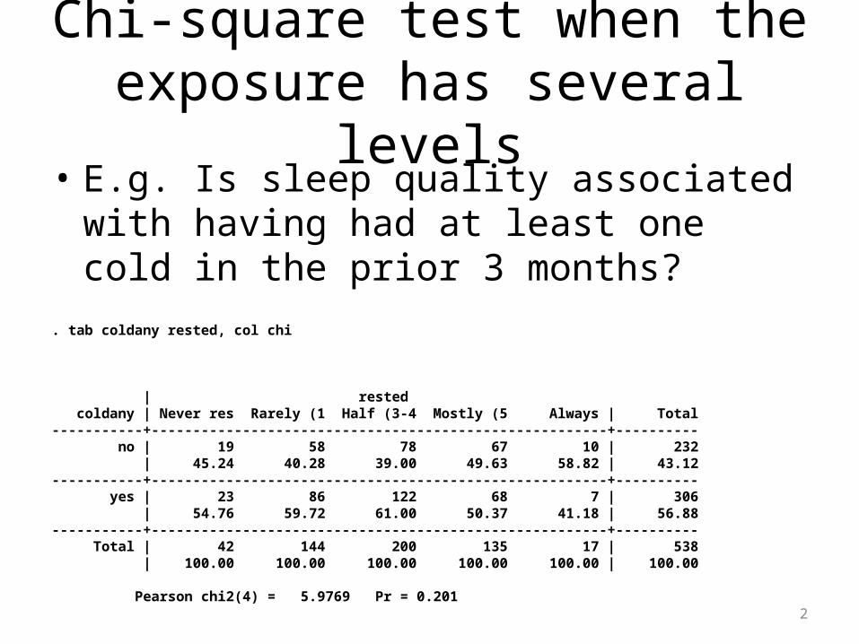
Chi-square test when the exposure has several levels
• E.g. Is sleep quality associated with having had at least one cold in the prior 3 months?
. tab coldany rested, col chi
| rested coldany | Never res Rarely (1 Half (3-4 Mostly (5 Always | Total-----------+-------------------------------------------------------+---------- no | 19 58 78 67 10 | 232 | 45.24 40.28 39.00 49.63 58.82 | 43.12 -----------+-------------------------------------------------------+---------- yes | 23 86 122 68 7 | 306 | 54.76 59.72 61.00 50.37 41.18 | 56.88 -----------+-------------------------------------------------------+---------- Total | 42 144 200 135 17 | 538 | 100.00 100.00 100.00 100.00 100.00 | 100.00
Pearson chi2(4) = 5.9769 Pr = 0.201
2
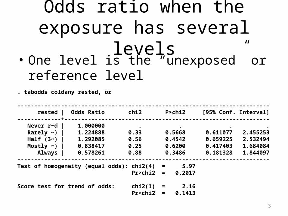
Odds ratio when the exposure has several levels
• One level is the “unexposed” or reference level
. tabodds coldany rested, or
--------------------------------------------------------------------------- rested | Odds Ratio chi2 P>chi2 [95% Conf. Interval]-------------+------------------------------------------------------------- Never r~d | 1.000000 . . . . Rarely ~) | 1.224888 0.33 0.5668 0.611077 2.455253 Half (3~) | 1.292085 0.56 0.4542 0.659225 2.532494 Mostly ~) | 0.838417 0.25 0.6200 0.417403 1.684084 Always | 0.578261 0.88 0.3486 0.181328 1.844097---------------------------------------------------------------------------Test of homogeneity (equal odds): chi2(4) = 5.97 Pr>chi2 = 0.2017
Score test for trend of odds: chi2(1) = 2.16 Pr>chi2 = 0.1413
3
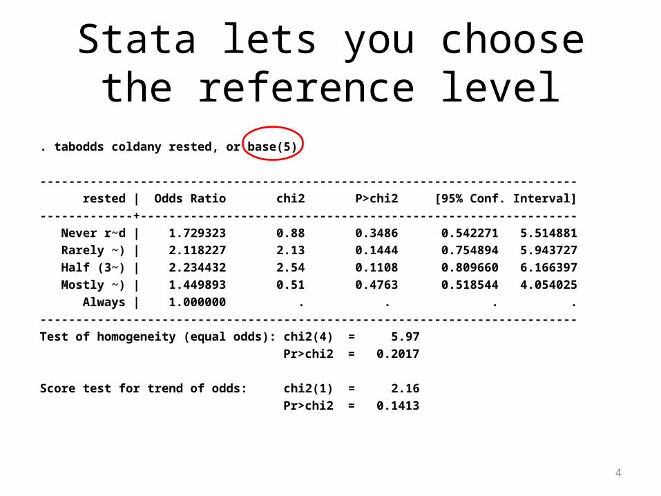
Stata lets you choose the reference level
. tabodds coldany rested, or base(5)
---------------------------------------------------------------------------
rested | Odds Ratio chi2 P>chi2 [95% Conf. Interval]
-------------+-------------------------------------------------------------
Never r~d | 1.729323 0.88 0.3486 0.542271 5.514881
Rarely ~) | 2.118227 2.13 0.1444 0.754894 5.943727
Half (3~) | 2.234432 2.54 0.1108 0.809660 6.166397
Mostly ~) | 1.449893 0.51 0.4763 0.518544 4.054025
Always | 1.000000 . . . .
---------------------------------------------------------------------------
Test of homogeneity (equal odds): chi2(4) = 5.97
Pr>chi2 = 0.2017
Score test for trend of odds: chi2(1) = 2.16
Pr>chi2 = 0.1413
4

Scatterplot
• Back to continuous outcomes• T-test, ANOVA, Wilcoxon rank-sum test,
Kruskal-Wallis test compare 2 or more independent samples– e.g. BMI by sex or alcohol consumption category
• The scatterplot is a simple method to examine the relationship between 2 continuous variables
Pagano and Gauvreau, Chapter 17 5
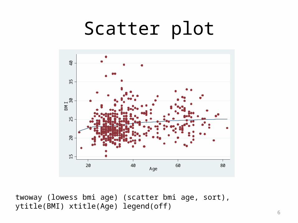
Scatter plot
twoway (lowess bmi age) (scatter bmi age, sort), ytitle(BMI) xtitle(Age) legend(off)
6
15
20
25
30
35
40
BM
I
20 40 60 80Age
Correlation
• Correlation is a method to examine the relationship between 2 continuous variables– Does one increase with the other?
• E.g. Does BMI decrease with total minutes of exercise?• Both variables are measured on the same people
(or unit of analysis)• Correlation assumes a linear relationship
between the two variables• Correlation is symmetric
– The correlation of A with B is the same as the correlation of B with A
Pagano and Gauvreau, Chapter 17 7
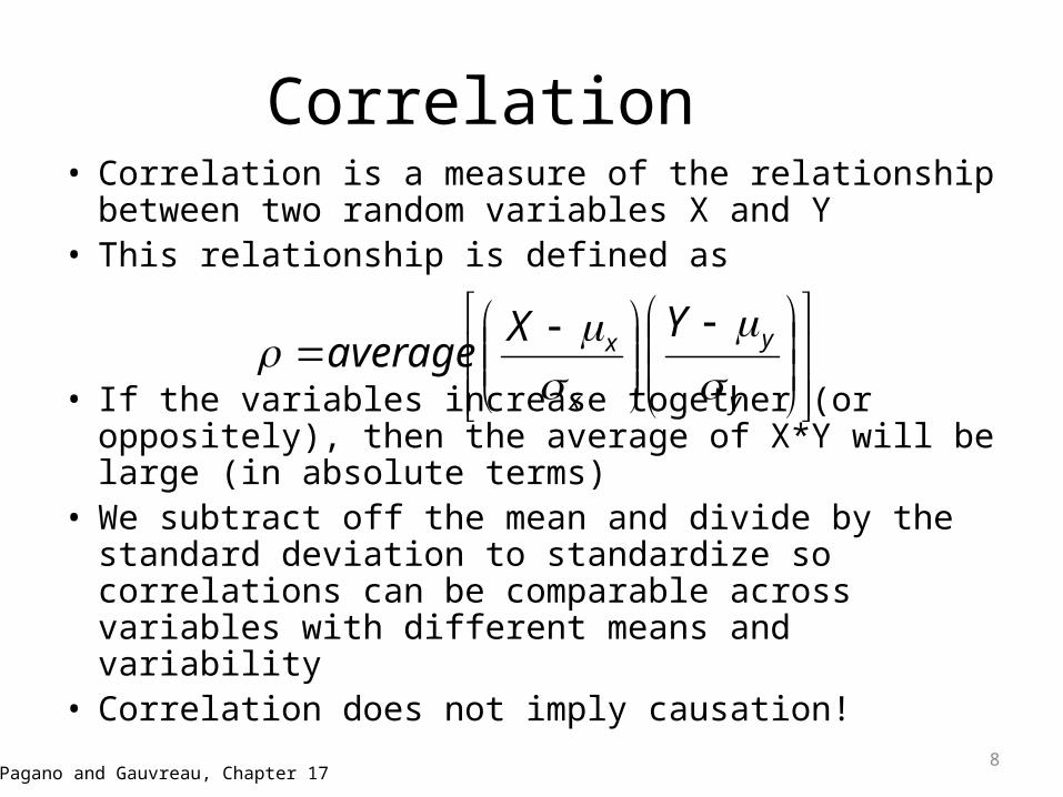
Correlation• Correlation is a measure of the relationship between
two random variables X and Y• This relationship is defined as
• If the variables increase together (or oppositely), then the average of X*Y will be large (in absolute terms)
• We subtract off the mean and divide by the standard deviation to standardize so correlations can be comparable across variables with different means and variability
• Correlation does not imply causation!Pagano and Gauvreau, Chapter 17
8
y
y
x
xYX
average
Correlation
9
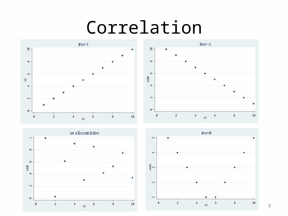
02
46
81
0x2
0 2 4 6 8 10x1
rho=1
02
46
81
0va
r8
0 2 4 6 8 10x1
rho=-1
12
34
5u
var
0 2 4 6 8 10x1
rho=0
0.2
.4.6
.81
var6
0 2 4 6 8 10x1
small correlation
Correlation
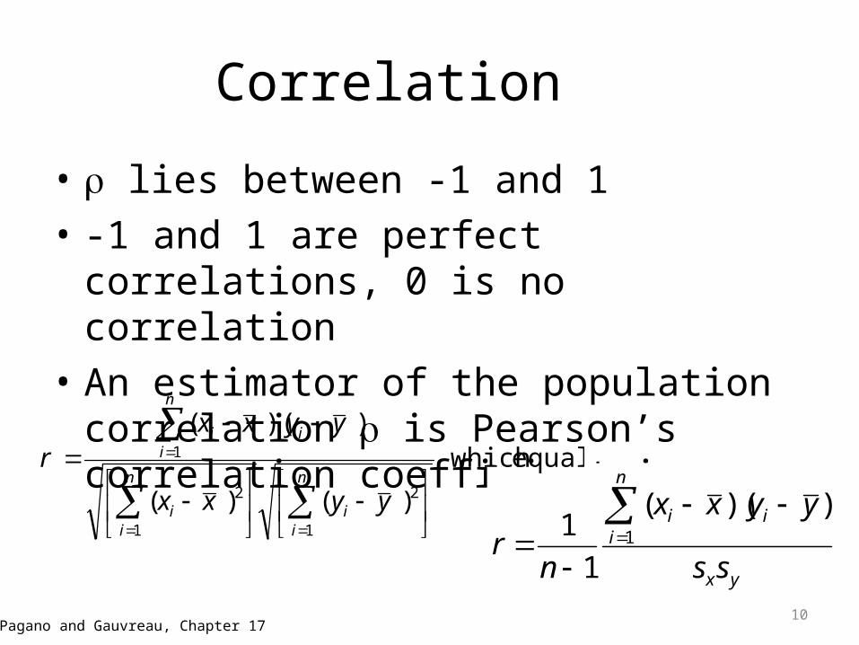
• lies between -1 and 1• -1 and 1 are perfect correlations, 0 is no
correlation• An estimator of the population correlation is
Pearson’s correlation coefficient is r
Pagano and Gauvreau, Chapter 17
yx
n
iii
ss
yyxx
nr
1
))((
1
1
10
equals which
)()(
))((
2
1
2
1
1
n
ii
n
ii
i
n
ii
yyxx
yyxxr
Correlation: hypothesis testing
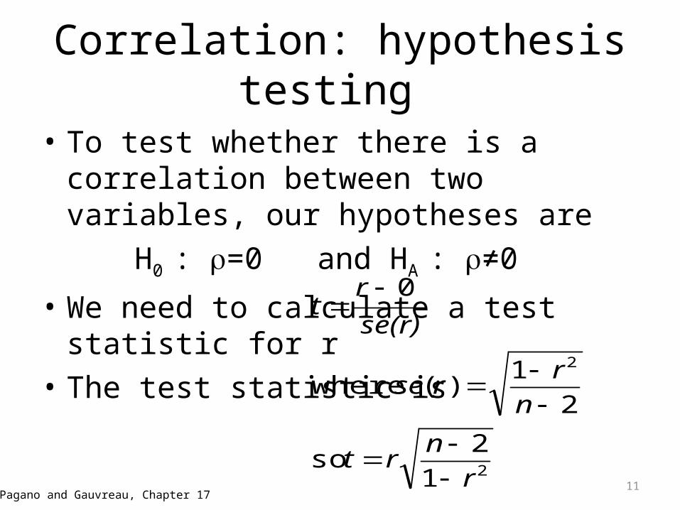
• To test whether there is a correlation between two variables, our hypotheses are
H0 : =0 and HA : ≠0
• We need to calculate a test statistic for r• The test statistic is
Pagano and Gauvreau, Chapter 1711
2
2
1
2 so
2
1)( where
0
r
nrt
n
rrse
se(r)
rt
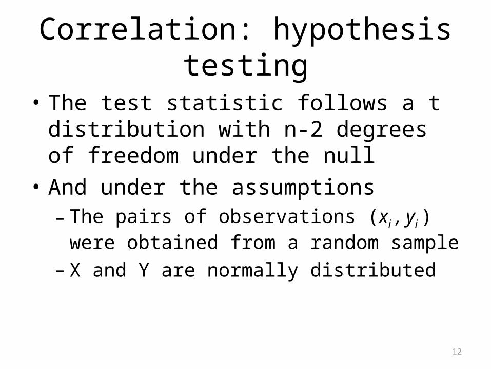
Correlation: hypothesis testing
• The test statistic follows a t distribution with n-2 degrees of freedom under the null
• And under the assumptions– The pairs of observations (xi , yi ) were obtained
from a random sample– X and Y are normally distributed
12
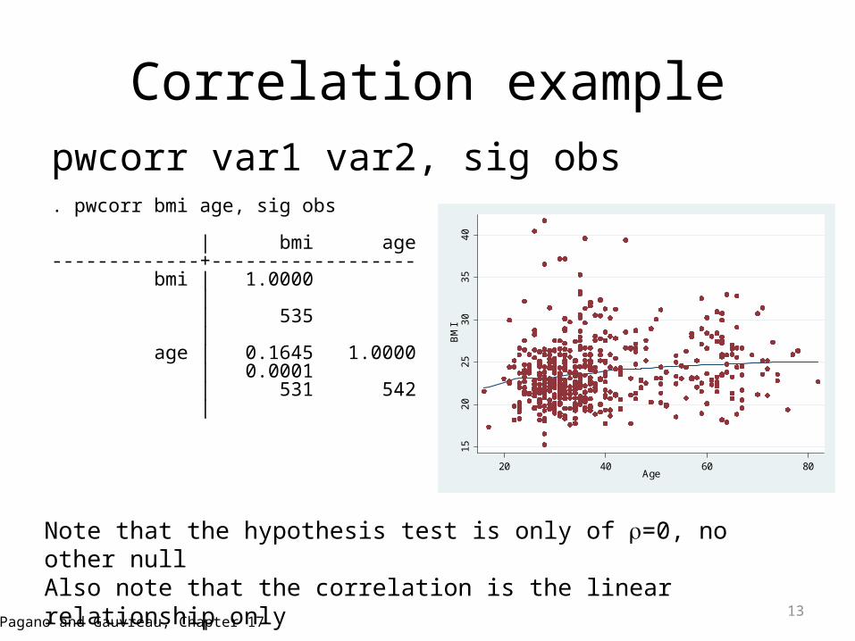
Correlation examplepwcorr var1 var2, sig obs. pwcorr bmi age, sig obs
| bmi age-------------+------------------ bmi | 1.0000 | | 535 | age | 0.1645 1.0000 | 0.0001 | 531 542 |
Pagano and Gauvreau, Chapter 1713
15
20
25
30
35
40
BM
I20 40 60 80
Age
Note that the hypothesis test is only of =0, no other nullAlso note that the correlation is the linear relationship only
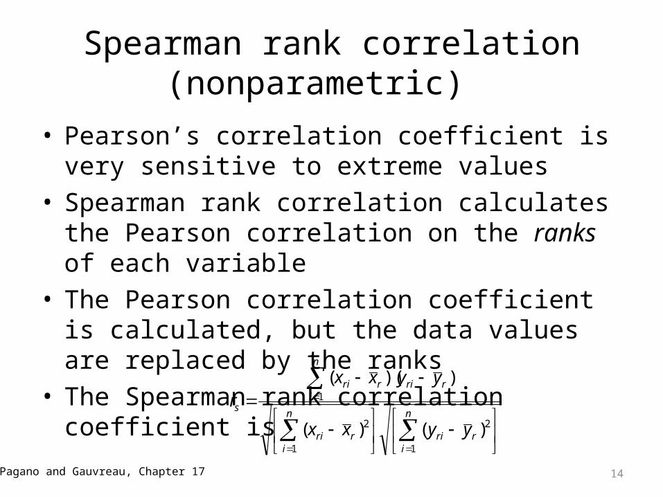
Spearman rank correlation (nonparametric)
• Pearson’s correlation coefficient is very sensitive to extreme values
• Spearman rank correlation calculates the Pearson correlation on the ranks of each variable
• The Pearson correlation coefficient is calculated, but the data values are replaced by the ranks
• The Spearman rank correlation coefficient is
Pagano and Gauvreau, Chapter 17 14
2
1
2
1
1
)()(
))((
n
irri
n
irri
rri
n
irri
s
yyxx
yyxxr
Spearman rank correlation (nonparametric)
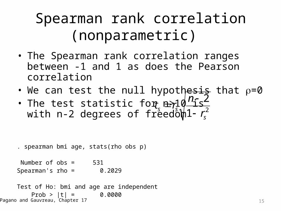
• The Spearman rank correlation ranges between -1 and 1 as does the Pearson correlation
• We can test the null hypothesis that =0• The test statistic for n>10 is
with n-2 degrees of freedom
. spearman bmi age, stats(rho obs p)
Number of obs = 531Spearman's rho = 0.2029
Test of Ho: bmi and age are independent Prob > |t| = 0.0000
Pagano and Gauvreau, Chapter 17 15
21
2
sss r
nrt
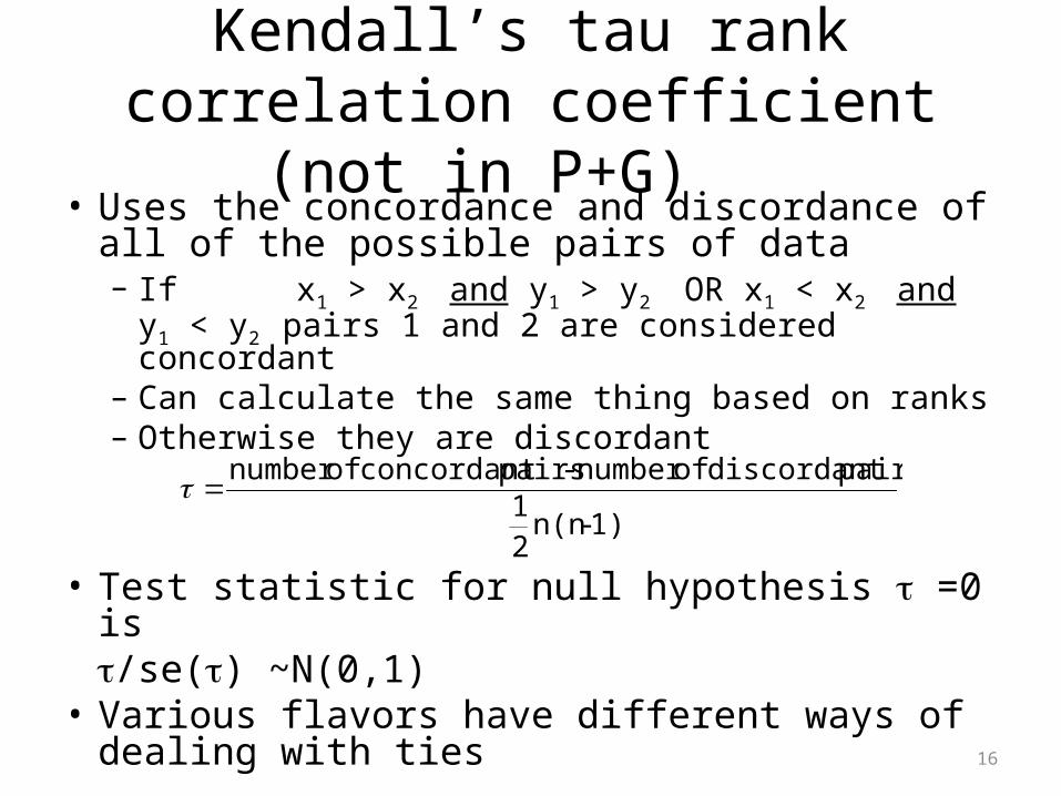
Kendall’s tau rank correlation coefficient (not in P+G)
• Uses the concordance and discordance of all of the possible pairs of data– If x1 > x2 and y1 > y2 OR x1 < x2 and y1 < y2 pairs 1
and 2 are considered concordant– Can calculate the same thing based on ranks– Otherwise they are discordant
• Test statistic for null hypothesis =0 is /se() ~N(0,1)
• Various flavors have different ways of dealing with ties
16
1)-n(n21
pairs discordant ofnumber - pairs concordant ofnumber
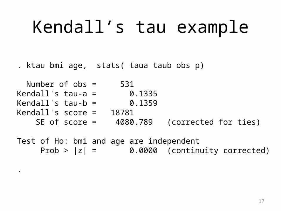
Kendall’s tau example
. ktau bmi age, stats( taua taub obs p)
Number of obs = 531Kendall's tau-a = 0.1335Kendall's tau-b = 0.1359Kendall's score = 18781 SE of score = 4080.789 (corrected for ties)
Test of Ho: bmi and age are independent Prob > |z| = 0.0000 (continuity corrected)
.
17
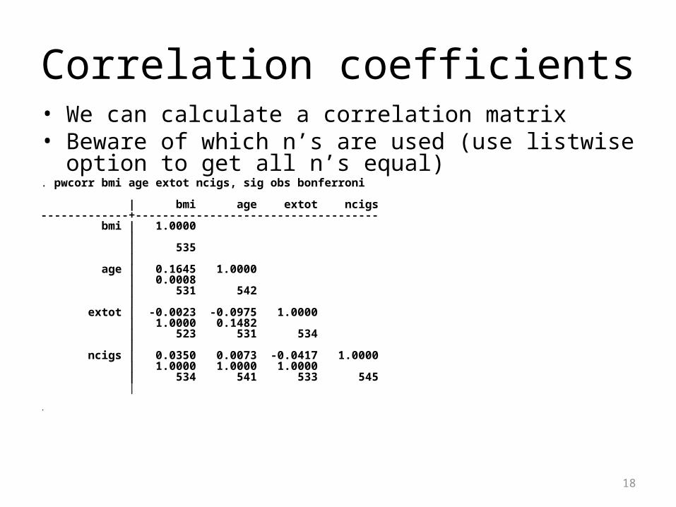
Correlation coefficients• We can calculate a correlation matrix• Beware of which n’s are used (use listwise option to get all n’s
equal). pwcorr bmi age extot ncigs, sig obs bonferroni
| bmi age extot ncigs-------------+------------------------------------ bmi | 1.0000 | | 535 | age | 0.1645 1.0000 | 0.0008 | 531 542 | extot | -0.0023 -0.0975 1.0000 | 1.0000 0.1482 | 523 531 534 | ncigs | 0.0350 0.0073 -0.0417 1.0000 | 1.0000 1.0000 1.0000 | 534 541 533 545 |
.
18
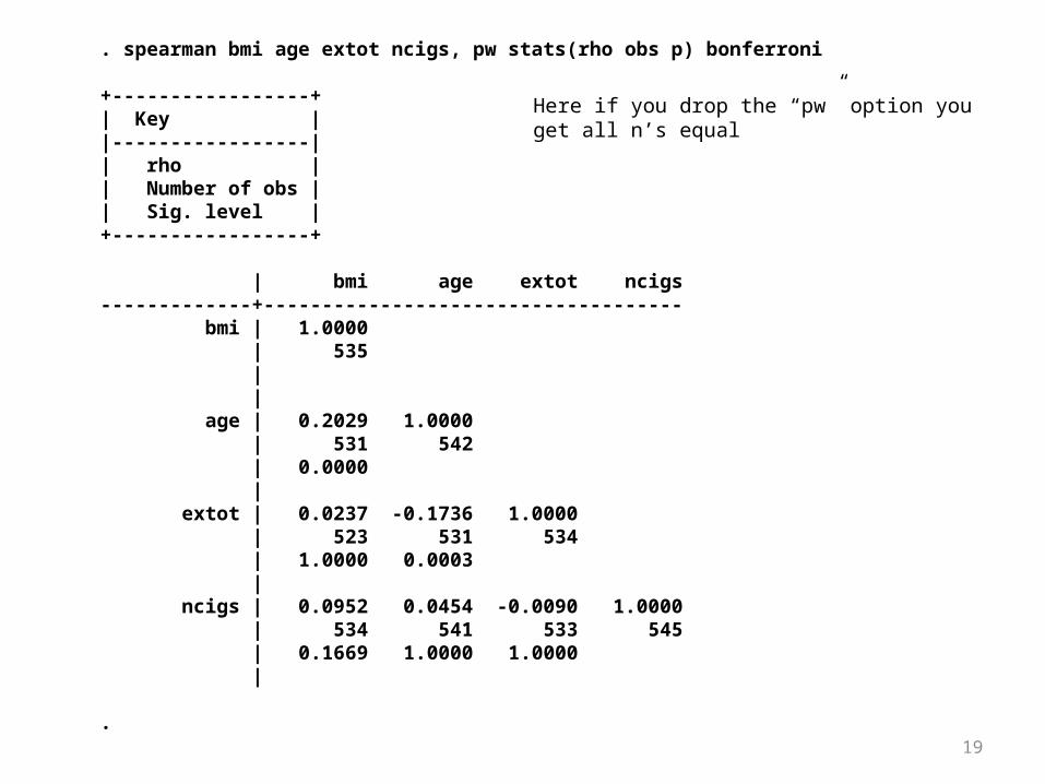
. spearman bmi age extot ncigs, pw stats(rho obs p) bonferroni
+-----------------+| Key ||-----------------|| rho || Number of obs || Sig. level |+-----------------+
| bmi age extot ncigs-------------+------------------------------------ bmi | 1.0000 | 535 | | age | 0.2029 1.0000 | 531 542 | 0.0000 | extot | 0.0237 -0.1736 1.0000 | 523 531 534 | 1.0000 0.0003 | ncigs | 0.0952 0.0454 -0.0090 1.0000 | 534 541 533 545 | 0.1669 1.0000 1.0000 |
. 19
Here if you drop the “pw” option you get all n’s equal
Simple linear regression
• Correlation allows us to quantify a linear relationship between two variables
• Regression allows us to additionally estimate how a change in a random variable X corresponds to a change in random variable Y
20
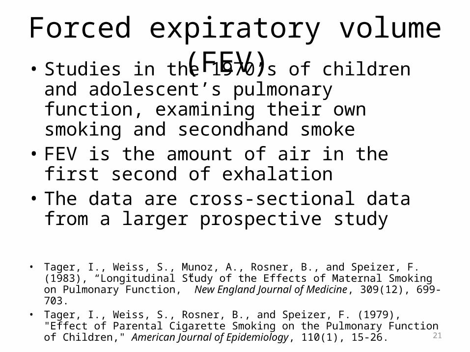
Forced expiratory volume (FEV) • Studies in the 1970’s of children and
adolescent’s pulmonary function, examining their own smoking and secondhand smoke
• FEV is the amount of air in the first second of exhalation
• The data are cross-sectional data from a larger prospective study
• Tager, I., Weiss, S., Munoz, A., Rosner, B., and Speizer, F. (1983), “Longitudinal Study of the Effects of Maternal Smoking on Pulmonary Function,” New England Journal of Medicine, 309(12), 699-703.
• Tager, I., Weiss, S., Rosner, B., and Speizer, F. (1979), "Effect of Parental Cigarette Smoking on the Pulmonary Function of Children," American Journal of Epidemiology, 110(1), 15-26. 21
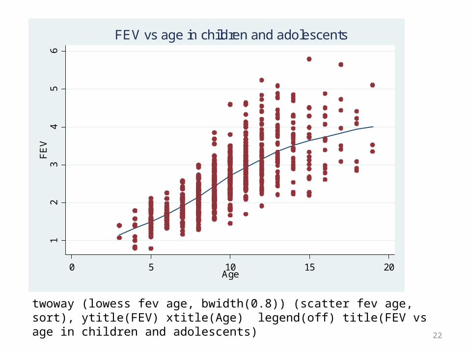
22
12
34
56
FE
V
0 5 10 15 20Age
FEV vs age in children and adolescents
twoway (lowess fev age, bwidth(0.8)) (scatter fev age, sort), ytitle(FEV) xtitle(Age) legend(off) title(FEV vs age in children and adolescents)
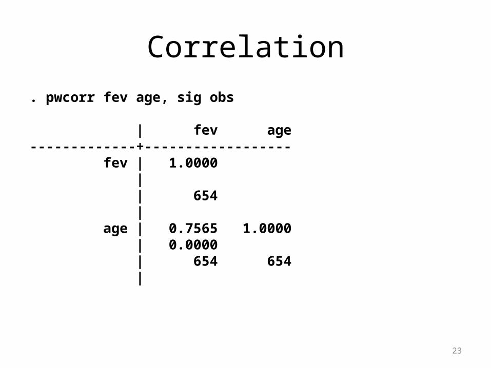
Correlation. pwcorr fev age, sig obs
| fev age-------------+------------------ fev | 1.0000 | | 654 | age | 0.7565 1.0000 | 0.0000 | 654 654 |
23
Concept of y|x and σy|x
• Consider to variables X and Y that are thought to be related
• You want to know how a change in X affects Y• Plot X versus Y, but instead of using all values of X,
categorize X into several categories• What you get would look like a boxplot of Y by the
grouped values of X• Each of the groups of X has a mean of Y y|x and a
standard deviation σy|x 24
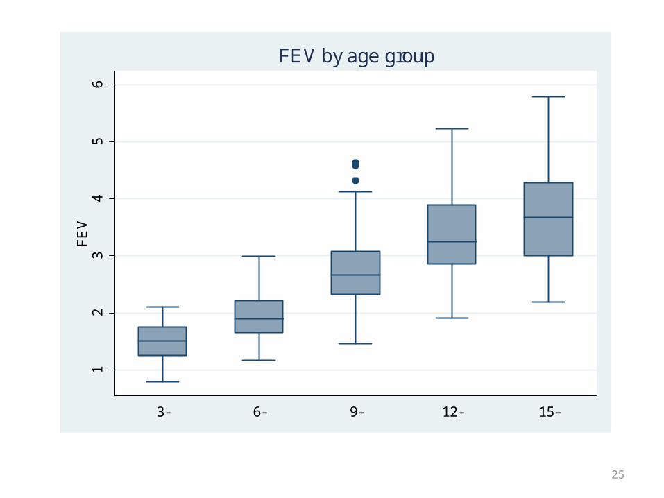
25
12
34
56
FE
V
3- 6- 9- 12- 15-
FEV by age group
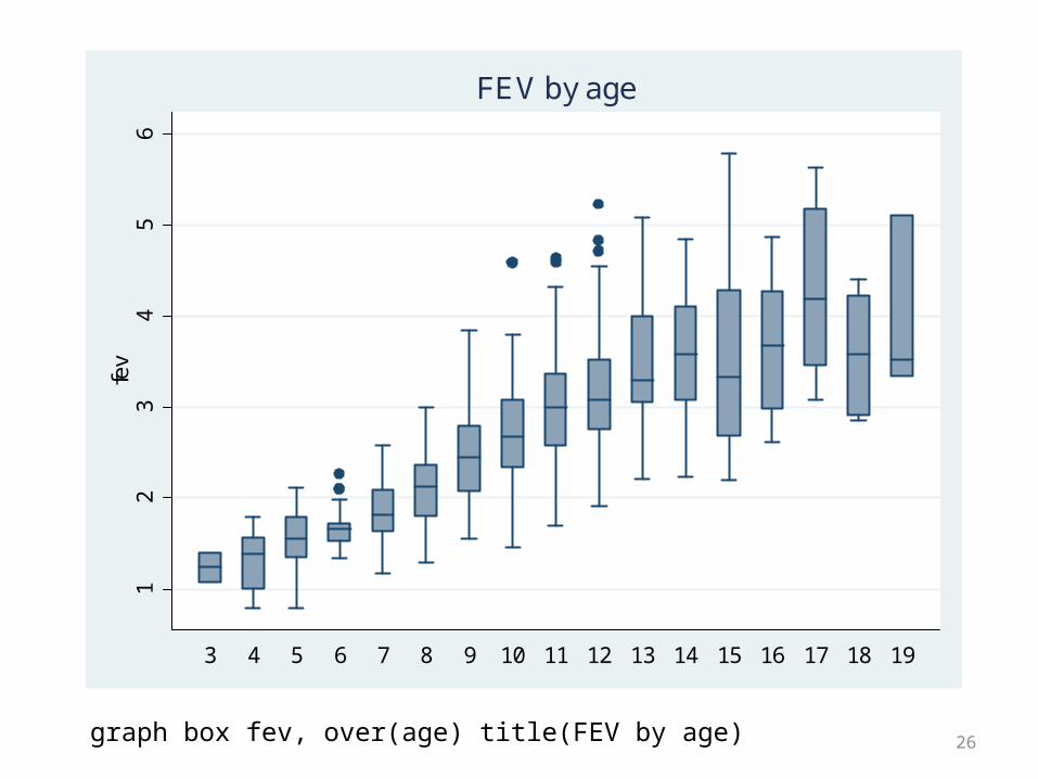
26
12
34
56
fev
3 4 5 6 7 8 9 10 11 12 13 14 15 16 17 18 19
FEV by age
graph box fev, over(age) title(FEV by age)
27
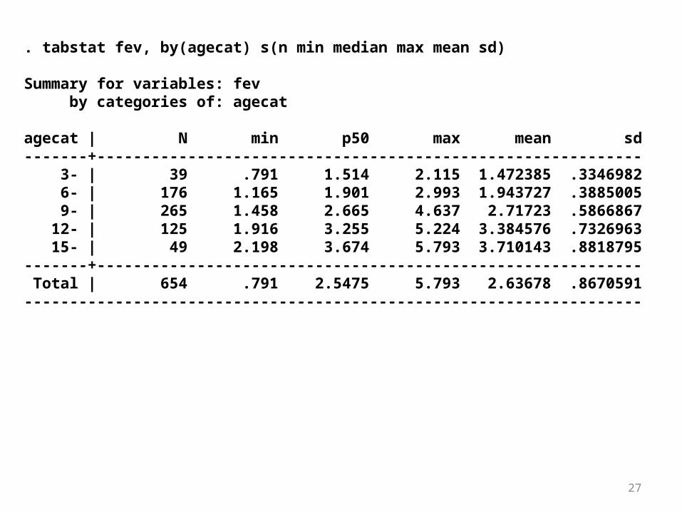
. tabstat fev, by(agecat) s(n min median max mean sd)
Summary for variables: fev by categories of: agecat
agecat | N min p50 max mean sd-------+------------------------------------------------------------ 3- | 39 .791 1.514 2.115 1.472385 .3346982 6- | 176 1.165 1.901 2.993 1.943727 .3885005 9- | 265 1.458 2.665 4.637 2.71723 .5866867 12- | 125 1.916 3.255 5.224 3.384576 .7326963 15- | 49 2.198 3.674 5.793 3.710143 .8818795-------+------------------------------------------------------------ Total | 654 .791 2.5475 5.793 2.63678 .8670591--------------------------------------------------------------------
Simple linear regression
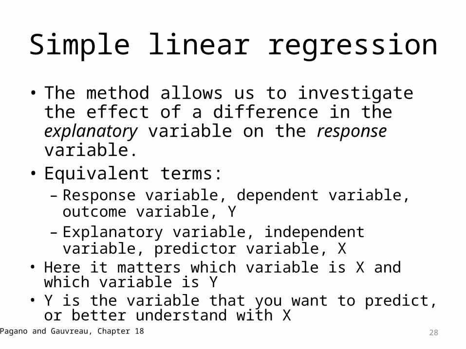
• The method allows us to investigate the effect of a difference in the explanatory variable on the response variable.
• Equivalent terms: – Response variable, dependent variable, outcome
variable, Y– Explanatory variable, independent variable, predictor
variable, X• Here it matters which variable is X and which variable is Y• Y is the variable that you want to predict, or better
understand with X
Pagano and Gauvreau, Chapter 18 28
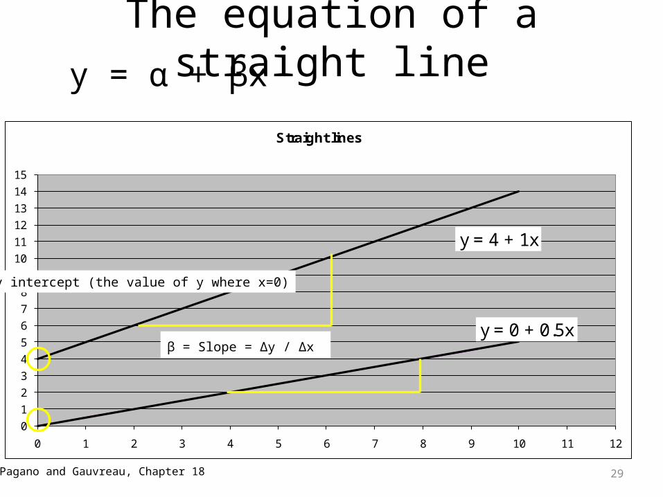
The equation of a straight line
y = 4 + 1x
y = 0 + 0.5x
0
1
2
3
4
5
6
7
8
9
10
11
12
13
14
15
0 1 2 3 4 5 6 7 8 9 10 11 12
Straight lines
α = y intercept (the value of y where x=0)
β = Slope = Δy / Δx
y = α + βx
Pagano and Gauvreau, Chapter 18 29
Simple linear regression
• Population regression equation μy|x = α + x• This is the equation of a straight line• α and are constants and are called the coefficients
of the equation• α is the y-intercept and which is the mean value of Y
when X=0, which is μy|0 • The slope is the change in the mean value of y that
corresponds to a one-unit increase in x• E.g. X=3 vs. X=2
μy|3 - μy|2 = (α + *3 ) – (α + *2) =
Pagano and Gauvreau, Chapter 18 30
Simple linear regression• Even if there is a linear relationship between Y and X in
theory, there will be some variability in the population• At each value of X, there is a range of Y values, with a mean
μy|x and a standard deviation σy|x • So when we model the data, we note this by including an
error term, ε, in our regression equation
• The linear regression equation is y = α + x + ε• The error, ε, is the distance a sample value y has from the
population regression line y = α + x + ε
μy|x = α + x so y- μy|x = ε
Pagano and Gauvreau, Chapter 18 31
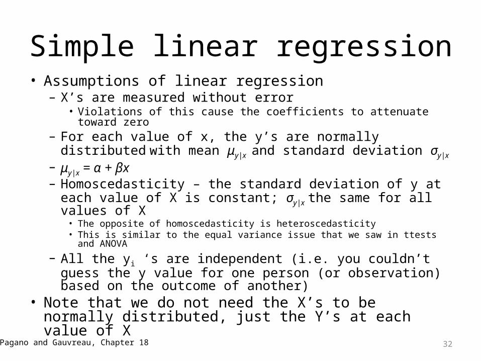
Simple linear regression• Assumptions of linear regression
– X’s are measured without error• Violations of this cause the coefficients to attenuate toward zero
– For each value of x, the y’s are normally distributed with mean μy|x and standard deviation σy|x
– μy|x = α + βx – Homoscedasticity – the standard deviation of y at each
value of X is constant; σy|x the same for all values of X • The opposite of homoscedasticity is heteroscedasticity• This is similar to the equal variance issue that we saw in ttests and ANOVA
– All the yi ‘s are independent (i.e. you couldn’t guess the y value for one person (or observation) based on the outcome of another)
• Note that we do not need the X’s to be normally distributed, just the Y’s at each value of XPagano and Gauvreau, Chapter 18 32
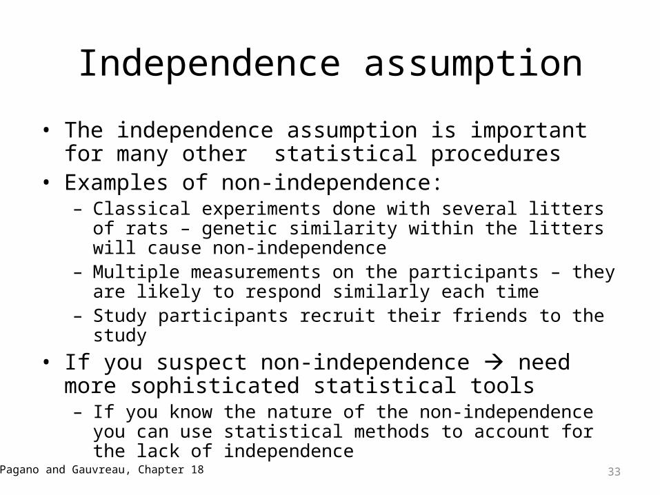
Independence assumption
• The independence assumption is important for many other statistical procedures
• Examples of non-independence:– Classical experiments done with several litters of rats – genetic
similarity within the litters will cause non-independence– Multiple measurements on the participants – they are likely to
respond similarly each time– Study participants recruit their friends to the study
• If you suspect non-independence need more sophisticated statistical tools– If you know the nature of the non-independence you can use
statistical methods to account for the lack of independence
Pagano and Gauvreau, Chapter 18 33
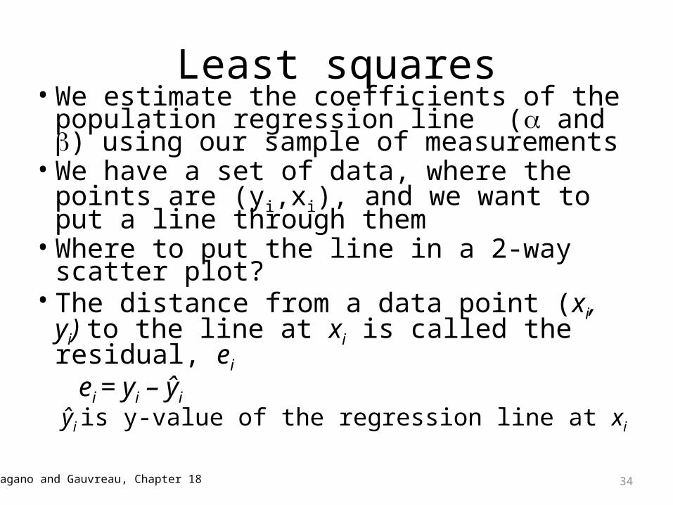
Least squares• We estimate the coefficients of the
population regression line ( and ) using our sample of measurements
• We have a set of data, where the points are (yi,xi), and we want to put a line through them
• Where to put the line in a 2-way scatter plot?
• The distance from a data point (xi, yi) to the line at xi is called the residual, ei
ei = yi – ŷiŷi is y-value of the regression line at xiPagano and Gauvreau, Chapter 18 34
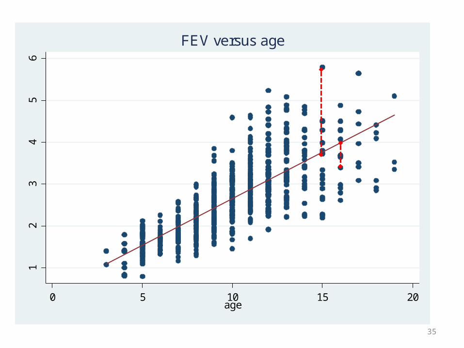
35
12
34
56
0 5 10 15 20age
FEV versus age
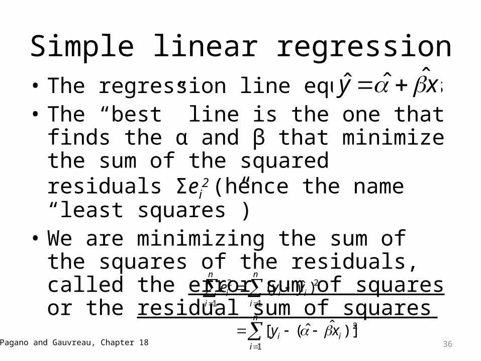
Simple linear regression• The regression line equation is • The “best” line is the one that finds the α and
β that minimize the sum of the squared residuals Σei
2 (hence the name “least squares”)• We are minimizing the sum of the squares of
the residuals, called the error sum of squares or the residual sum of squares
Pagano and Gauvreau, Chapter 18 36
xy ˆˆˆ
n
iii
n
iii
n
ii
xy
yye
1
2
1
2
1
2
)]ˆˆ([
)ˆ(
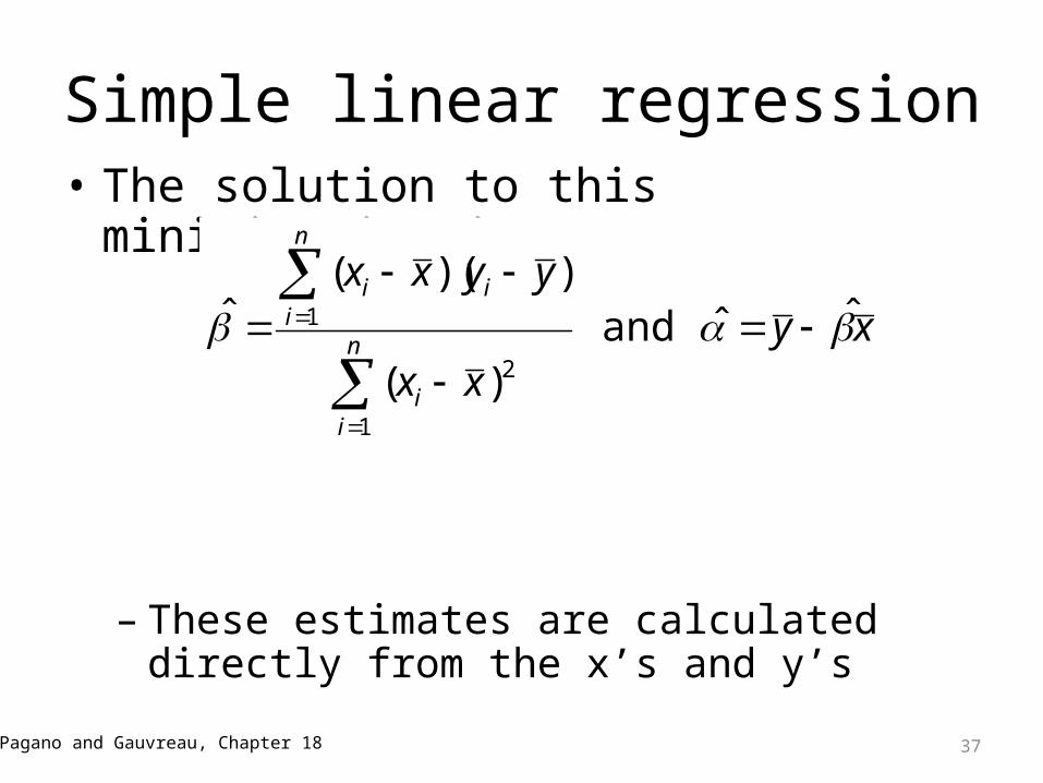
Simple linear regression• The solution to this minimization is
– These estimates are calculated directly from the x’s and y’s
xyxx
yyxx
n
ii
n
iii
ˆˆ and )(
))((ˆ
1
2
1
Pagano and Gauvreau, Chapter 18 37
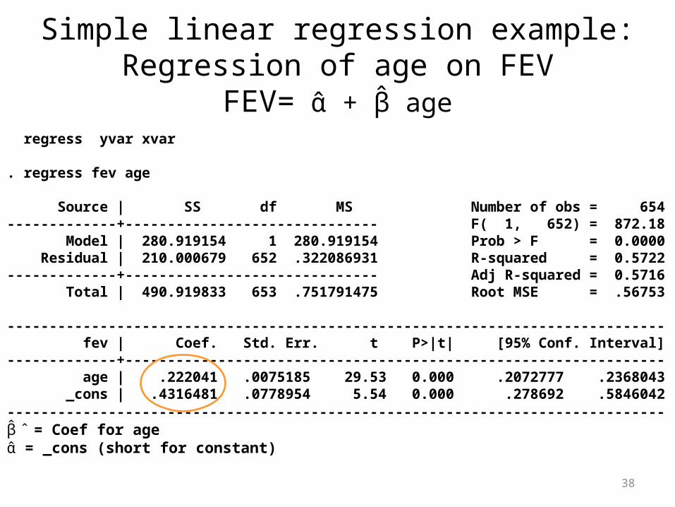
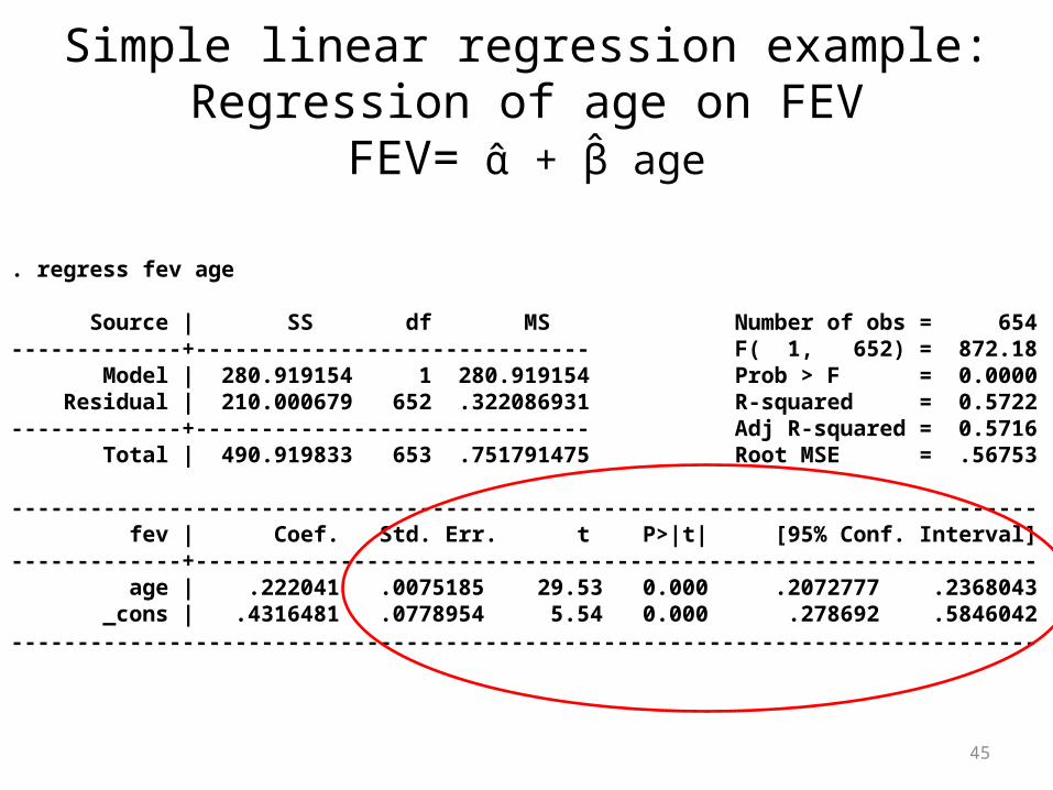
Simple linear regression example: Regression of age on FEV
FEV= + ageα̂� β̂� regress yvar xvar
. regress fev age
Source | SS df MS Number of obs = 654-------------+------------------------------ F( 1, 652) = 872.18 Model | 280.919154 1 280.919154 Prob > F = 0.0000 Residual | 210.000679 652 .322086931 R-squared = 0.5722-------------+------------------------------ Adj R-squared = 0.5716 Total | 490.919833 653 .751791475 Root MSE = .56753
------------------------------------------------------------------------------ fev | Coef. Std. Err. t P>|t| [95% Conf. Interval]-------------+---------------------------------------------------------------- age | .222041 .0075185 29.53 0.000 .2072777 .2368043 _cons | .4316481 .0778954 5.54 0.000 .278692 .5846042------------------------------------------------------------------------------ β̂� � = Coef for age
α̂� = _cons (short for constant)
38
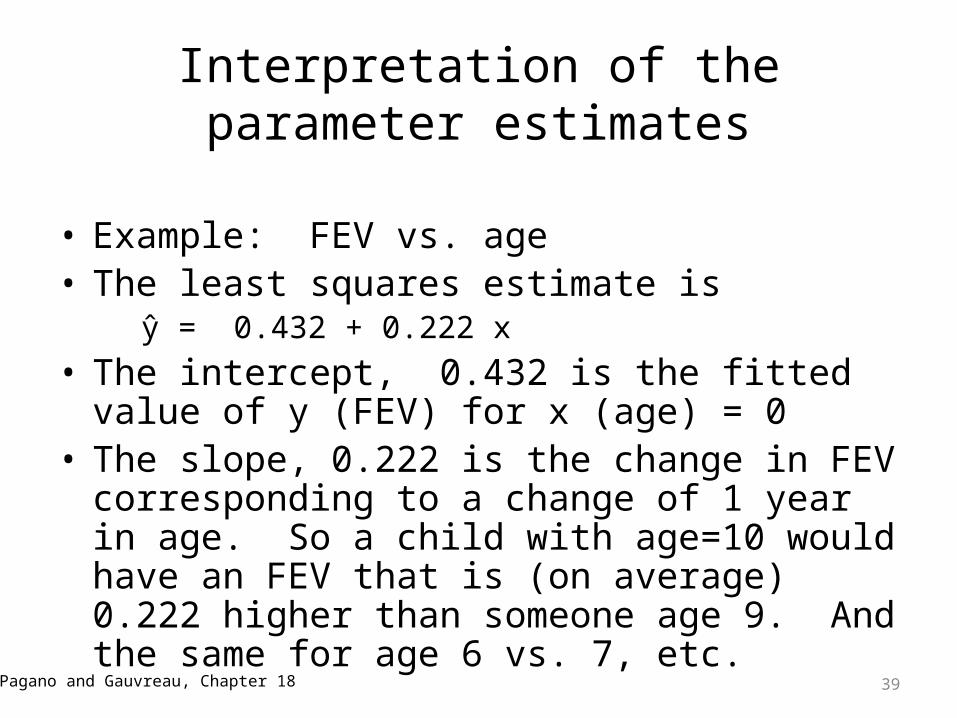
Interpretation of the parameter estimates
• Example: FEV vs. age• The least squares estimate is
ŷ = 0.432 + 0.222 x• The intercept, 0.432 is the fitted value of y (FEV) for
x (age) = 0• The slope, 0.222 is the change in FEV corresponding
to a change of 1 year in age. So a child with age=10 would have an FEV that is (on average) 0.222 higher than someone age 9. And the same for age 6 vs. 7, etc.
Pagano and Gauvreau, Chapter 18 39
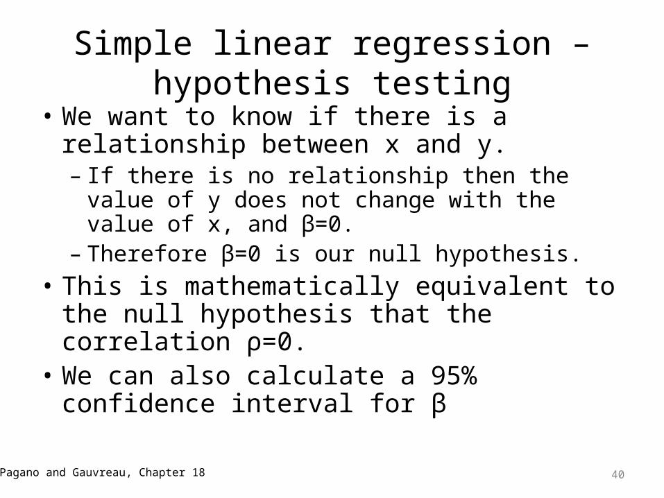
Simple linear regression – hypothesis testing
• We want to know if there is a relationship between x and y. – If there is no relationship then the value of y does
not change with the value of x, and β=0.– Therefore β=0 is our null hypothesis.
• This is mathematically equivalent to the null hypothesis that the correlation ρ=0.
• We can also calculate a 95% confidence interval for β
Pagano and Gauvreau, Chapter 18 40
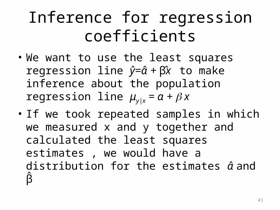
Inference for regression coefficients
• We want to use the least squares regression line ŷ= + α̂� βx � to make inference about the population regression line μy|x = α + x
• If we took repeated samples in which we measured x and y together and calculated the least squares estimates , we would have a distribution for the estimates α̂� and β̂�
41
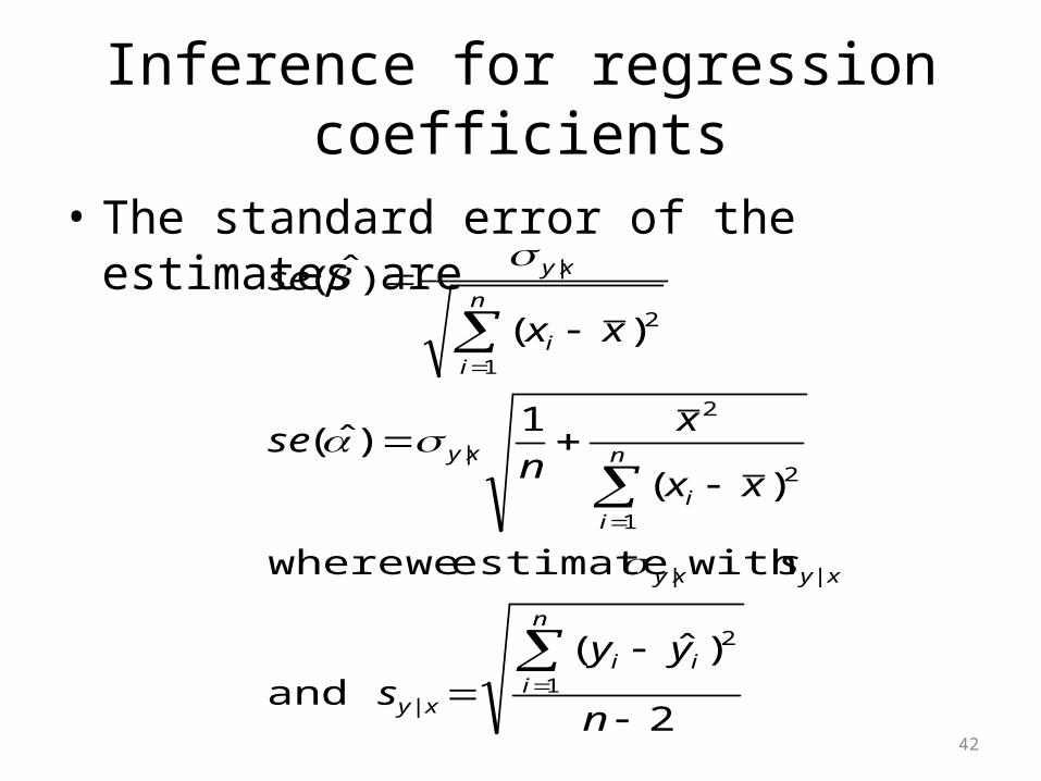
Inference for regression coefficients
• The standard error of the estimates are
422
)ˆ( and
with estimate wewhere
)(
1)ˆ(
)(
)ˆ(
1
2
|
1
2
2
|
1
2
|
n
yys
s
xx
x
nse
xx
se
n
iii
y|x
y|xxy
n
ii
xy
n
ii
xy
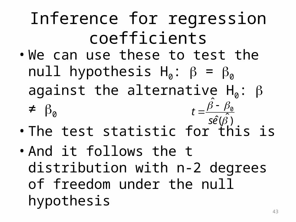
Inference for regression coefficients
• We can use these to test the null hypothesis H0: = 0 against the alternative H0: ≠ 0
• The test statistic for this is• And it follows the t distribution with n-2
degrees of freedom under the null hypothesis
43
)ˆ(ˆ
ˆ0
est
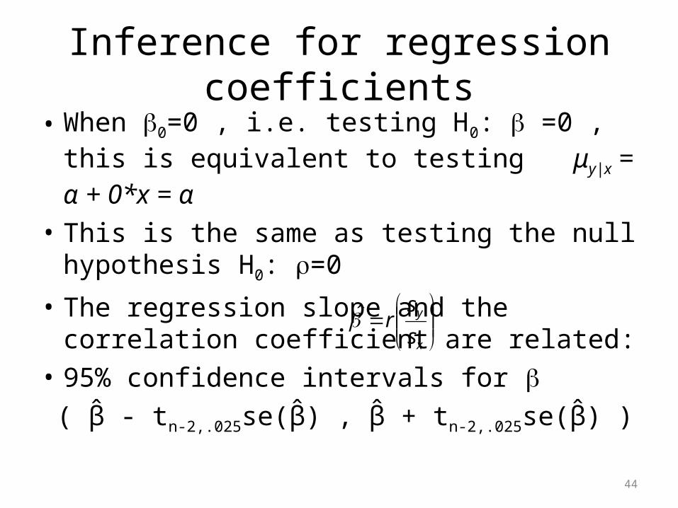
Inference for regression coefficients
• When 0=0 , i.e. testing H0: =0 , this is equivalent to testing μy|x = α + 0*x = α
• This is the same as testing the null hypothesis H0: =0
• The regression slope and the correlation coefficient are related:
• 95% confidence intervals for ( - tβ̂� n-2,.025se( ) , + tβ̂� β̂� n-2,.025se( ) ) β̂�
44
x
y
s
sr̂
Simple linear regression example: Regression of age on FEV
FEV= + ageα̂� β̂�
. regress fev age
Source | SS df MS Number of obs = 654-------------+------------------------------ F( 1, 652) = 872.18 Model | 280.919154 1 280.919154 Prob > F = 0.0000 Residual | 210.000679 652 .322086931 R-squared = 0.5722-------------+------------------------------ Adj R-squared = 0.5716 Total | 490.919833 653 .751791475 Root MSE = .56753
------------------------------------------------------------------------------ fev | Coef. Std. Err. t P>|t| [95% Conf. Interval]-------------+---------------------------------------------------------------- age | .222041 .0075185 29.53 0.000 .2072777 .2368043 _cons | .4316481 .0778954 5.54 0.000 .278692 .5846042------------------------------------------------------------------------------
45
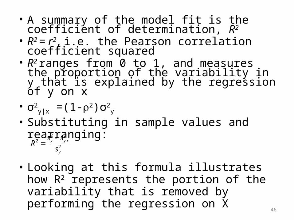
• A summary of the model fit is the coefficient of determination, R2
• R2 = r2 , i.e. the Pearson correlation coefficient squared
• R2 ranges from 0 to 1, and measures the proportion of the variability in y that is explained by the regression of y on x
• σ2y|x =(1-2)σ2
y
• Substituting in sample values and rearranging:
• Looking at this formula illustrates how R2 represents the portion of the variability that is removed by performing the regression on X
46
2
2|
22
y
xyy
s
ssR
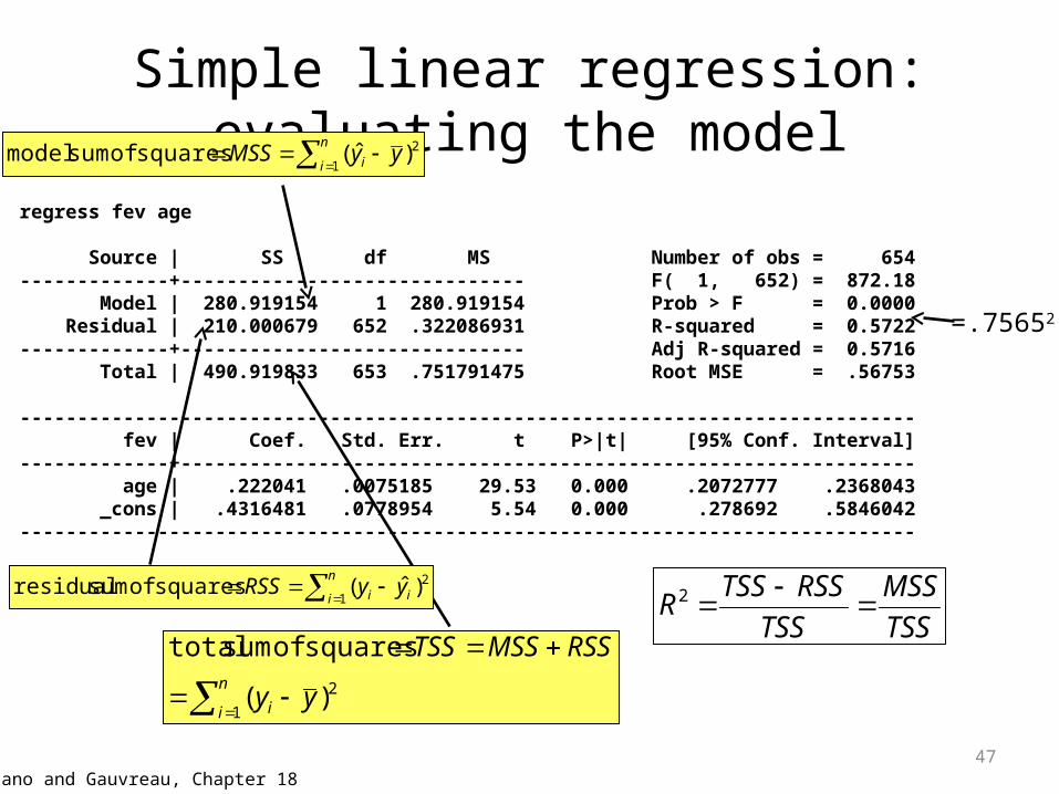
Simple linear regression: evaluating the model
regress fev age
Source | SS df MS Number of obs = 654-------------+------------------------------ F( 1, 652) = 872.18 Model | 280.919154 1 280.919154 Prob > F = 0.0000 Residual | 210.000679 652 .322086931 R-squared = 0.5722-------------+------------------------------ Adj R-squared = 0.5716 Total | 490.919833 653 .751791475 Root MSE = .56753
------------------------------------------------------------------------------ fev | Coef. Std. Err. t P>|t| [95% Conf. Interval]-------------+---------------------------------------------------------------- age | .222041 .0075185 29.53 0.000 .2072777 .2368043 _cons | .4316481 .0778954 5.54 0.000 .278692 .5846042------------------------------------------------------------------------------
Pagano and Gauvreau, Chapter 1847
=.75652
n
i i yyMSS1
2)ˆ( squares of sum model
n
i ii yyRSS1
2)ˆ( squares of sum residual
n
i i yy
RSSMSSTSS
1
2)(
squares of sum totalTSS
MSS
TSS
RSSTSSR
2
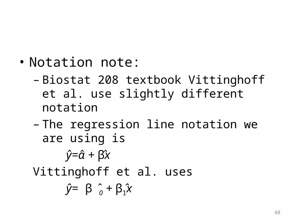
• Notation note:– Biostat 208 textbook Vittinghoff et al. use slightly
different notation– The regression line notation we are using is ŷ= + α̂� βx�Vittinghoff et al. uses ŷ= β �0 + β1x�
48

For next time
• Read Pagano and Gauvreau
– Pagano and Gauvreau Chapter 17-18 (review)– Pagano and Gauvreau Chapter 18-19
Related Documents