Bayesian Statistics for Genetics Lecture 1: Introduction

Bayesian Statistics for Genetics

Lecture 1: Introduction

Ken Rice

UW Dept of Biostatistics

July, 2016

Overview

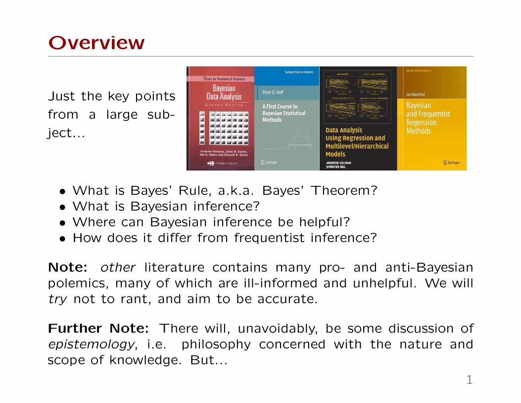
Just the key points

from a large sub-

ject...

• What is Bayes’ Rule, a.k.a. Bayes’ Theorem?• What is Bayesian inference?• Where can Bayesian inference be helpful?• How does it differ from frequentist inference?

Note: other literature contains many pro- and anti-Bayesianpolemics, many of which are ill-informed and unhelpful. We willtry not to rant, and aim to be accurate.

Further Note: There will, unavoidably, be some discussion ofepistemology, i.e. philosophy concerned with the nature andscope of knowledge. But...

1

Overview

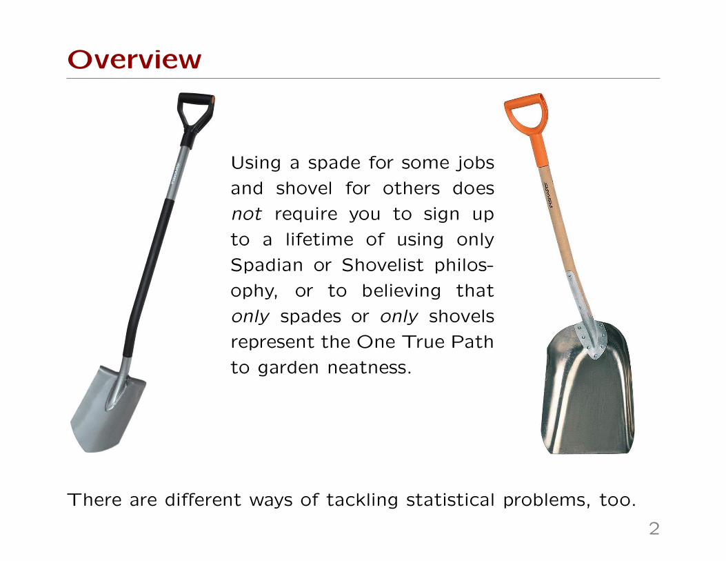
Using a spade for some jobs

and shovel for others does

not require you to sign up

to a lifetime of using only

Spadian or Shovelist philos-

ophy, or to believing that

only spades or only shovels

represent the One True Path

to garden neatness.

There are different ways of tackling statistical problems, too.

2

Bayes’ Theorem

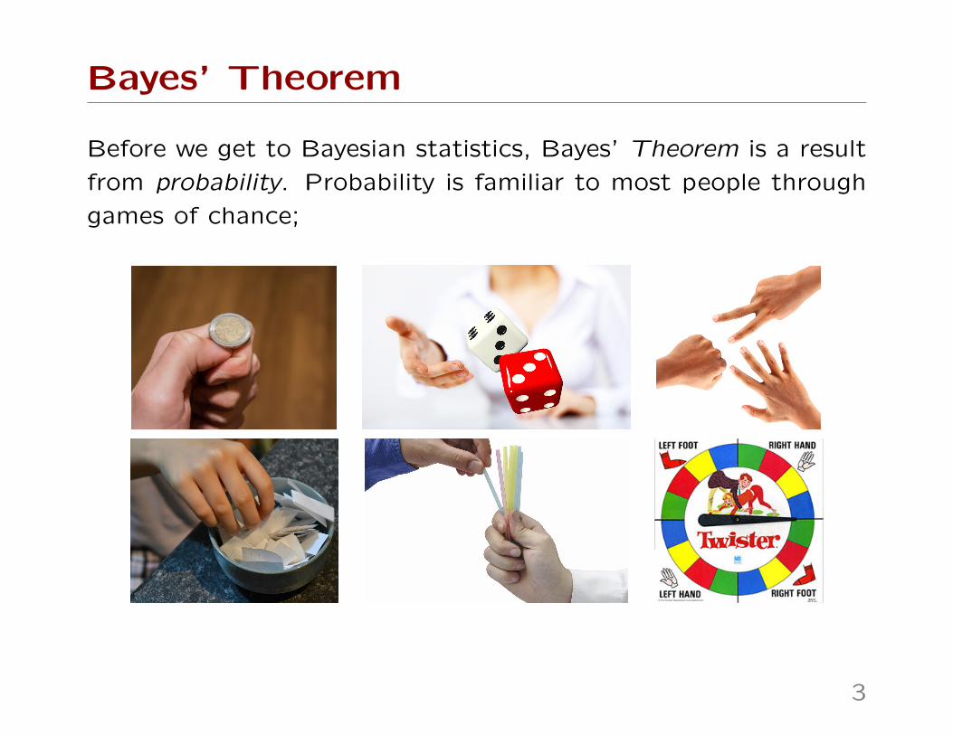
Before we get to Bayesian statistics, Bayes’ Theorem is a result

from probability. Probability is familiar to most people through

games of chance;

3

Bayes’ Theorem

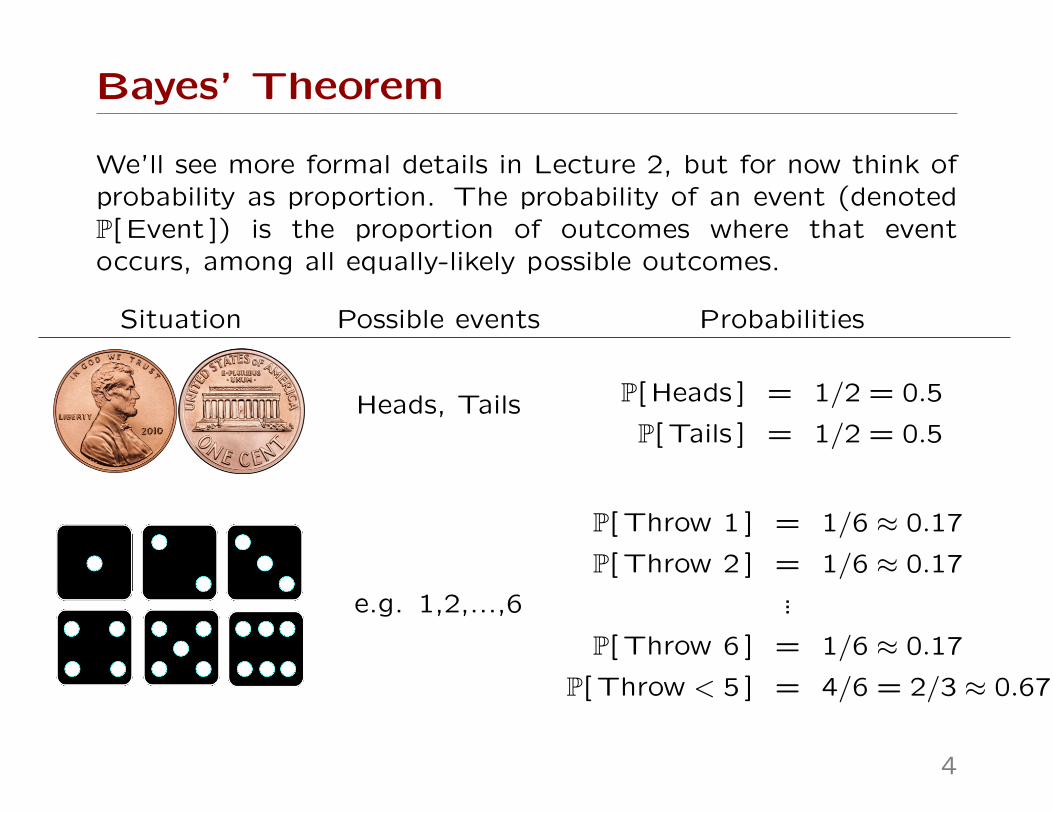
We’ll see more formal details in Lecture 2, but for now think ofprobability as proportion. The probability of an event (denotedP[ Event ]) is the proportion of outcomes where that eventoccurs, among all equally-likely possible outcomes.

Situation Possible events Probabilities

Heads, Tails P[ Heads ] = 1/2 = 0.5

P[ Tails ] = 1/2 = 0.5

e.g. 1,2,...,6

P[ Throw 1 ] = 1/6 ≈ 0.17

P[ Throw 2 ] = 1/6 ≈ 0.17...

P[ Throw 6 ] = 1/6 ≈ 0.17

P[ Throw < 5 ] = 4/6 = 2/3 ≈ 0.67

4

Bayes’ Theorem

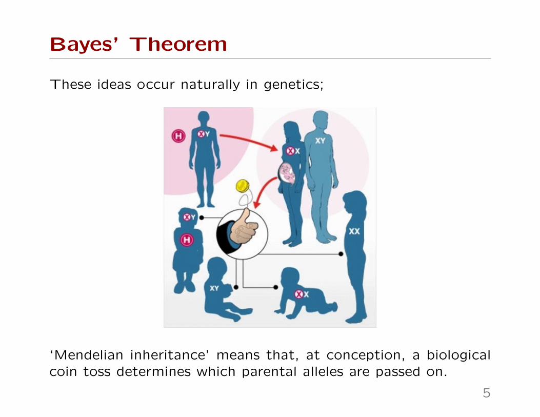
These ideas occur naturally in genetics;

‘Mendelian inheritance’ means that, at conception, a biologicalcoin toss determines which parental alleles are passed on.

5

Bayes’ Theorem

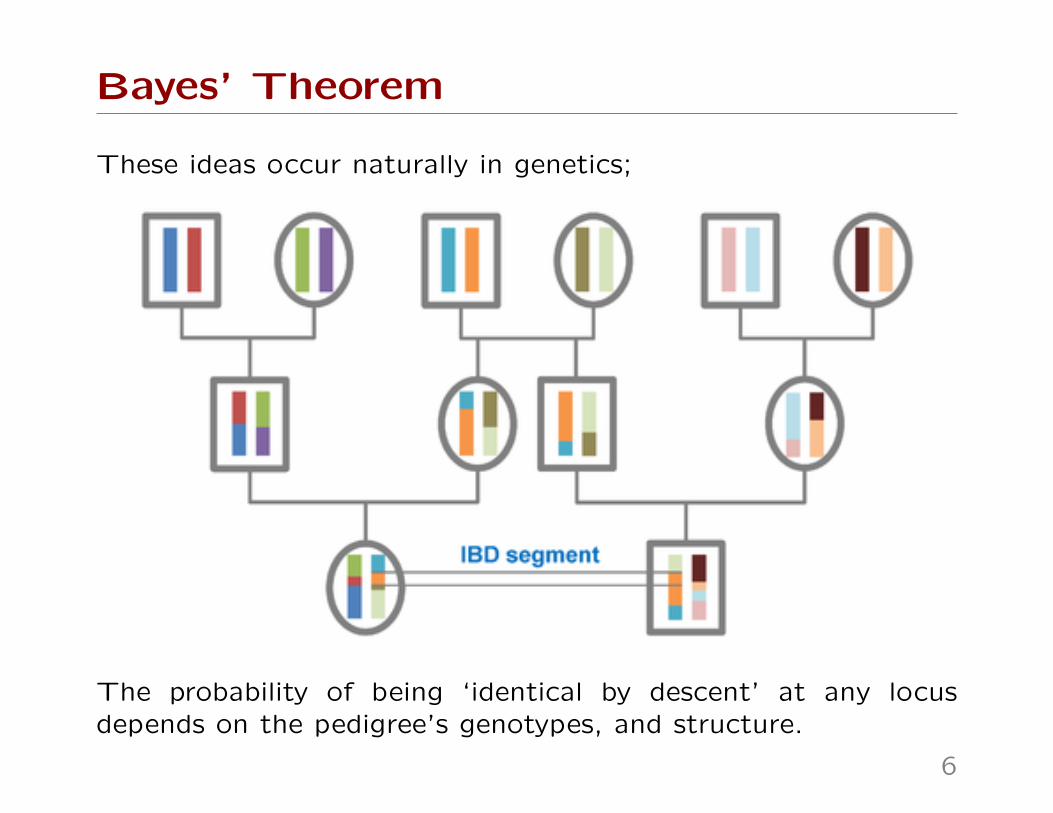
These ideas occur naturally in genetics;

The probability of being ‘identical by descent’ at any locusdepends on the pedigree’s genotypes, and structure.

6

Bayes’ Theorem

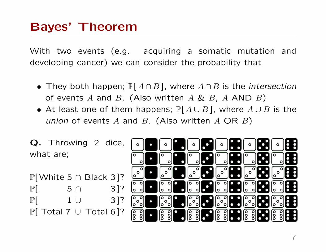
With two events (e.g. acquiring a somatic mutation and

developing cancer) we can consider the probability that

• They both happen; P[A∩B ], where A∩B is the intersection

of events A and B. (Also written A & B, A AND B)

• At least one of them happens; P[A ∪B ], where A ∪B is the

union of events A and B. (Also written A OR B)

Q. Throwing 2 dice,

what are;

P[ White 5 ∩ Black 3 ]?

P[ 5 ∩ 3 ]?

P[ 1 ∪ 3 ]?

P[ Total 7 ∪ Total 6 ]?

7

Bayes’ Theorem

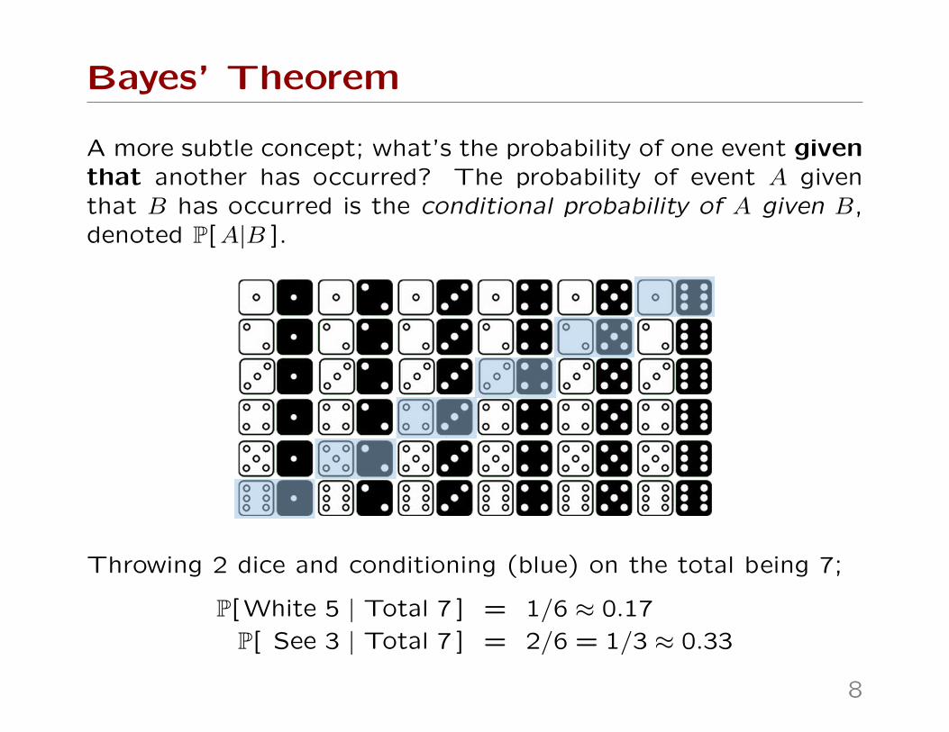
A more subtle concept; what’s the probability of one event giventhat another has occurred? The probability of event A giventhat B has occurred is the conditional probability of A given B,denoted P[A|B ].

Throwing 2 dice and conditioning (blue) on the total being 7;

P[ White 5 | Total 7 ] = 1/6 ≈ 0.17

P[ See 3 | Total 7 ] = 2/6 = 1/3 ≈ 0.33

8

Bayes’ Theorem

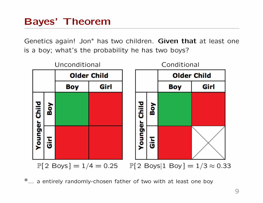
Genetics again! Jon∗ has two children. Given that at least one

is a boy; what’s the probability he has two boys?

Unconditional Conditional

P[ 2 Boys ] = 1/4 = 0.25 P[ 2 Boys|1 Boy ] = 1/3 ≈ 0.33

*... a entirely randomly-chosen father of two with at least one boy

9

Bayes’ Theorem

Now a problem to show that conditional probability can be non-

intuitive – NB this is not a ‘trick’ question;

Q. Jon has two children. Given that at least one is a boy who

was born on a Tuesday ; what’s the probability he has two boys?

• The ‘obvious’ (but wrong!) answer is to stick with 1/3.

What can Tuesday possibly have to do with it?

• It may help your intuition, to note that a boy being born on

a Tuesday is a (fairly) rare event;

– Having two sons would give Jon two chances of experi-

encing this rare event

– Having only one would give him one chance

– ‘Conditioning’ means we know this event occurred, i.e.

Jon was ‘lucky’ enough to have the event

• Easier Q. Is P[ 2 Boys|1 Tues Boy ] > 1/3? or < 1/3?

10

Bayes’ Theorem

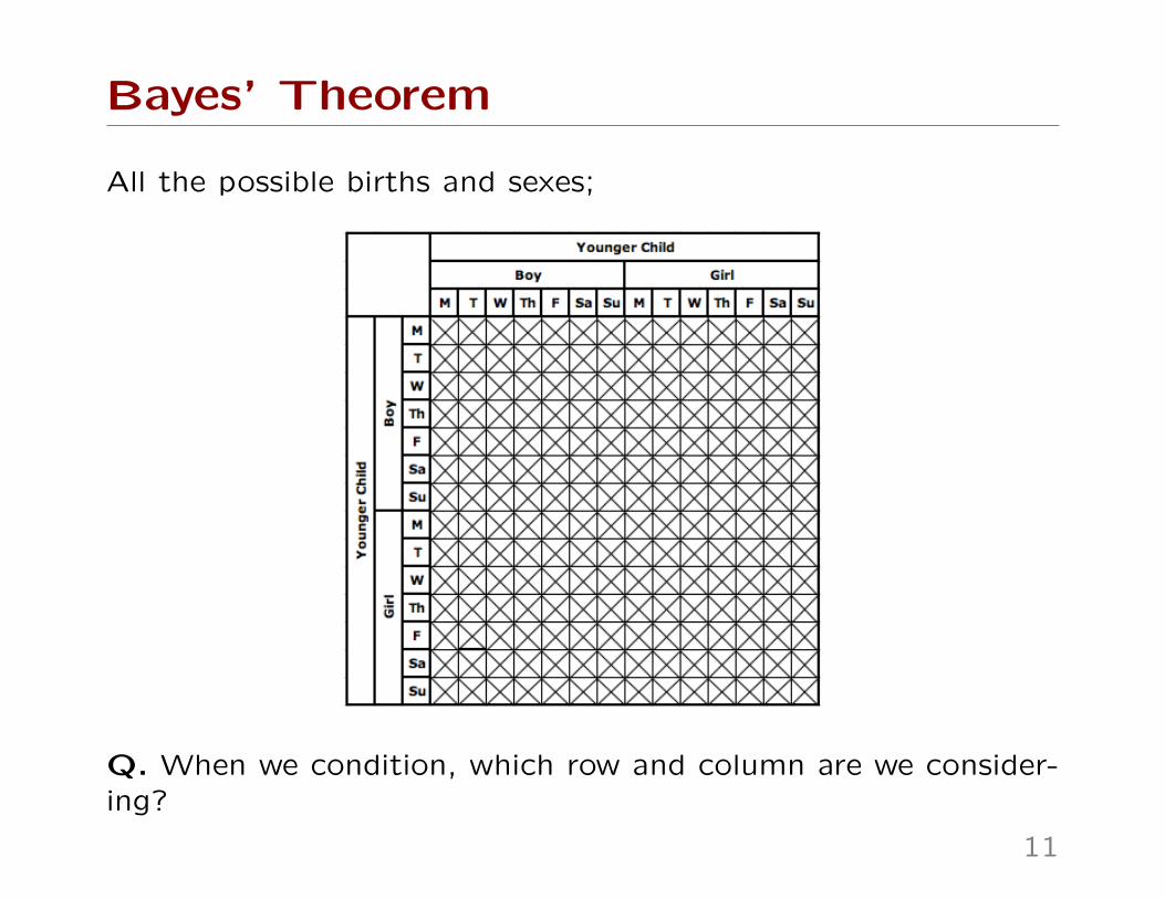
All the possible births and sexes;

Q. When we condition, which row and column are we consider-ing?

11

Bayes’ Theorem

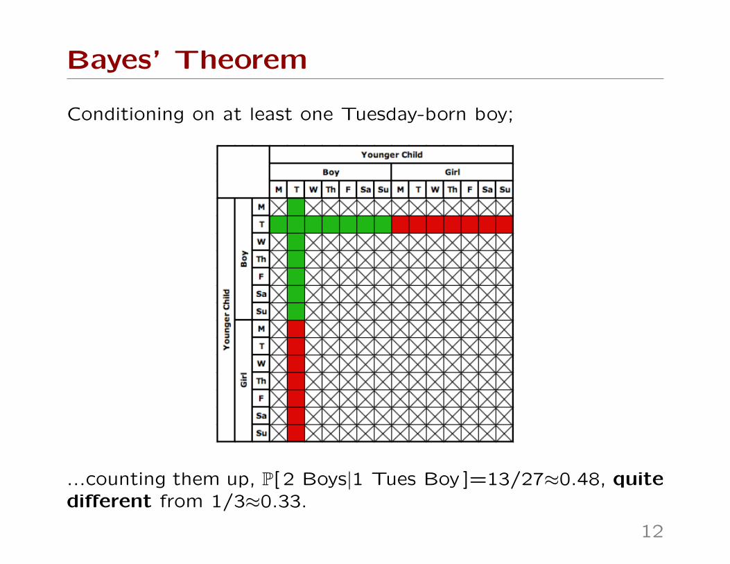
Conditioning on at least one Tuesday-born boy;

...counting them up, P[ 2 Boys|1 Tues Boy ]=13/27≈0.48, quitedifferent from 1/3≈0.33.

12

Bayes’ Theorem

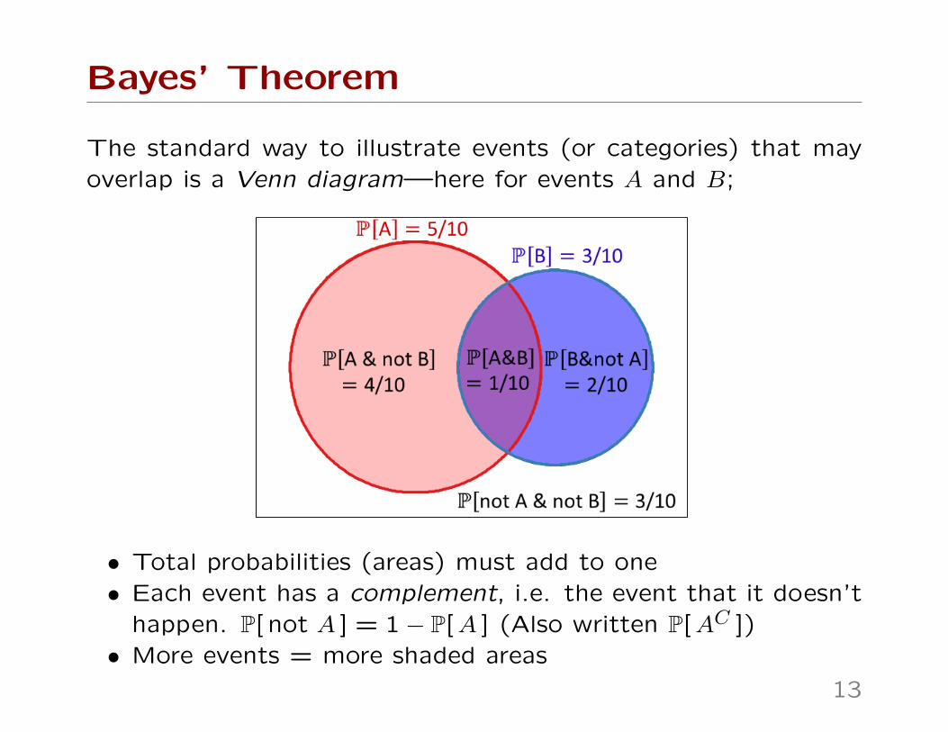
The standard way to illustrate events (or categories) that mayoverlap is a Venn diagram—here for events A and B;

• Total probabilities (areas) must add to one• Each event has a complement, i.e. the event that it doesn’t

happen. P[ not A ] = 1− P[A ] (Also written P[AC ])• More events = more shaded areas

13

Bayes’ Theorem

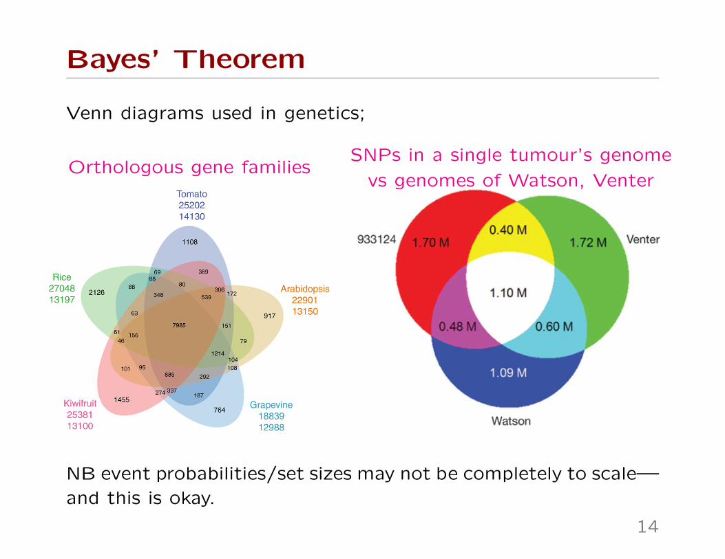
Venn diagrams used in genetics;

Orthologous gene familiesSNPs in a single tumour’s genome

vs genomes of Watson, Venter

NB event probabilities/set sizes may not be completely to scale—

and this is okay.

14

Bayes’ Theorem

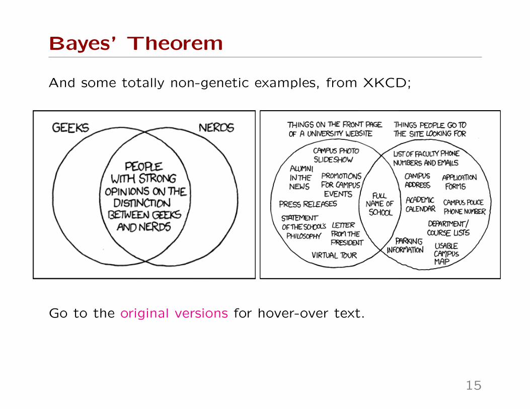
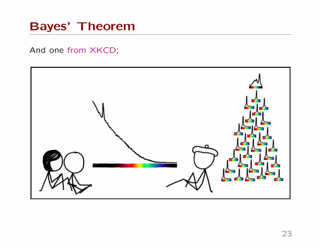
And some totally non-genetic examples, from XKCD;

Go to the original versions for hover-over text.

15

Bayes’ Theorem

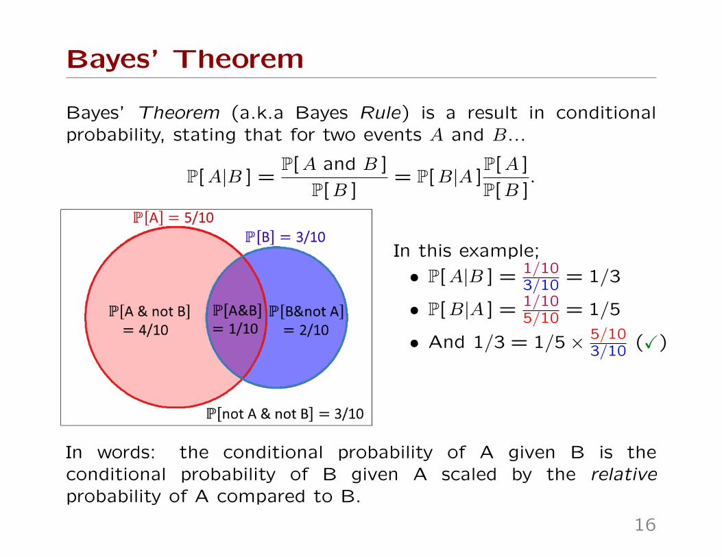
Bayes’ Theorem (a.k.a Bayes Rule) is a result in conditionalprobability, stating that for two events A and B...

P[A|B ] =P[A and B ]

P[B ]= P[B|A ]

P[A ]

P[B ].

In this example;

• P[A|B ] = 1/103/10 = 1/3

• P[B|A ] = 1/105/10 = 1/5

• And 1/3 = 1/5× 5/103/10 (X)

In words: the conditional probability of A given B is theconditional probability of B given A scaled by the relativeprobability of A compared to B.

16

Bayes’ Theorem

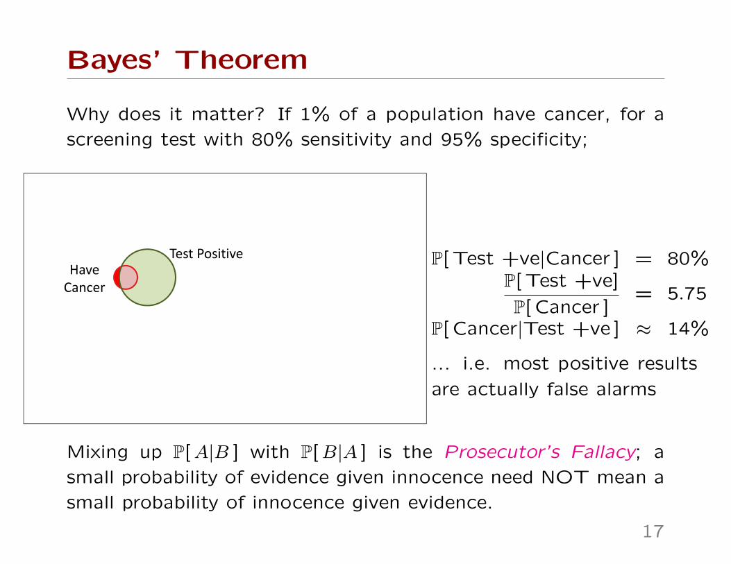
Why does it matter? If 1% of a population have cancer, for a

screening test with 80% sensitivity and 95% specificity;

Test PositiveHave Cancer

P[ Test +ve|Cancer ] = 80%P[ Test +ve]

P[ Cancer ]= 5.75

P[ Cancer|Test +ve ] ≈ 14%

... i.e. most positive results

are actually false alarms

Mixing up P[A|B ] with P[B|A ] is the Prosecutor’s Fallacy; a

small probability of evidence given innocence need NOT mean a

small probability of innocence given evidence.

17

Bayes’ Theorem: Sally Clark

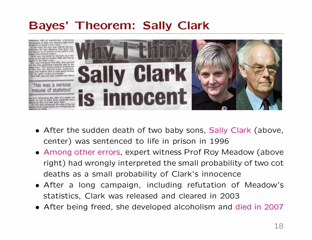
• After the sudden death of two baby sons, Sally Clark (above,

center) was sentenced to life in prison in 1996

• Among other errors, expert witness Prof Roy Meadow (above

right) had wrongly interpreted the small probability of two cot

deaths as a small probability of Clark’s innocence

• After a long campaign, including refutation of Meadow’s

statistics, Clark was released and cleared in 2003

• After being freed, she developed alcoholism and died in 2007

18

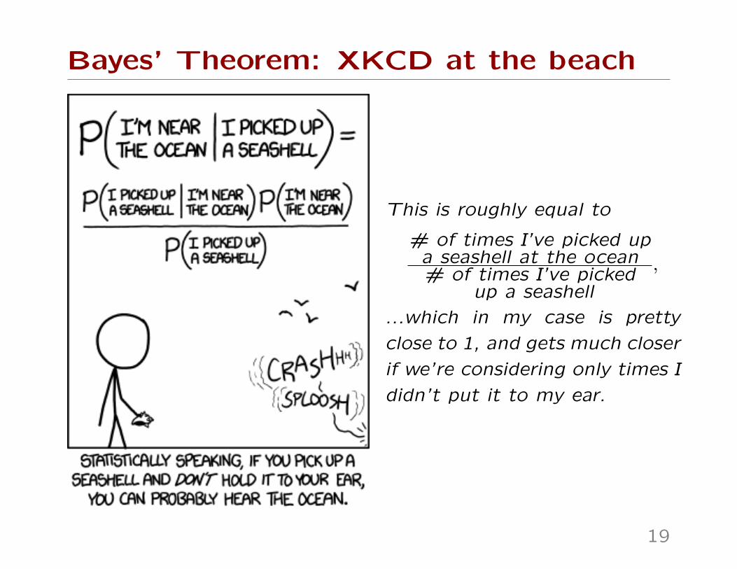
Bayes’ Theorem: XKCD at the beach

This is roughly equal to

# of times I’ve picked upa seashell at the ocean# of times I’ve picked

up a seashell

,

...which in my case is pretty

close to 1, and gets much closer

if we’re considering only times I

didn’t put it to my ear.

19

Bayes’ Theorem

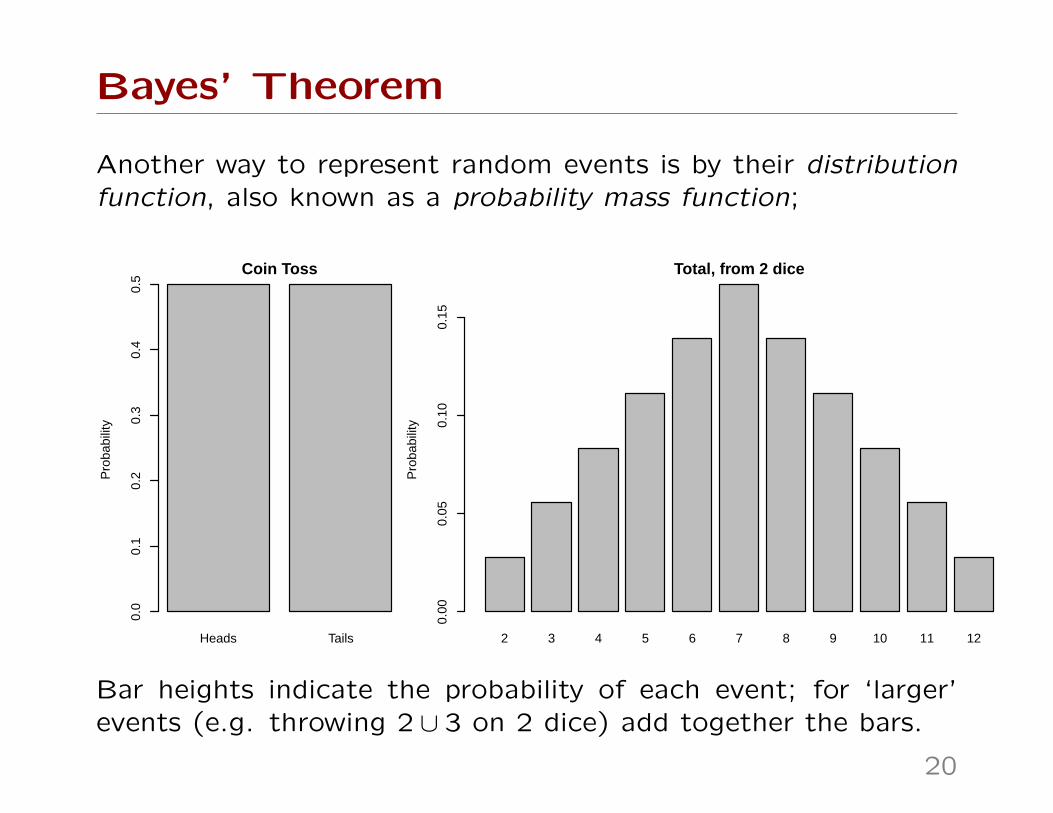
Another way to represent random events is by their distributionfunction, also known as a probability mass function;

Heads Tails

Coin Toss

Pro

babi

lity

0.0

0.1

0.2

0.3

0.4

0.5

2 3 4 5 6 7 8 9 10 11 12

Total, from 2 dice

Pro

babi

lity

0.00

0.05

0.10

0.15

Bar heights indicate the probability of each event; for ‘larger’events (e.g. throwing 2 ∪ 3 on 2 dice) add together the bars.

20

Bayes’ Theorem

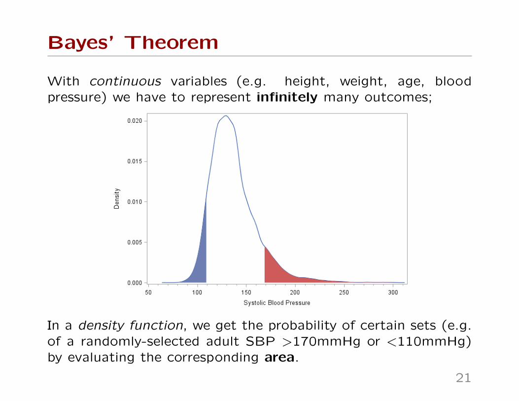
With continuous variables (e.g. height, weight, age, bloodpressure) we have to represent infinitely many outcomes;

In a density function, we get the probability of certain sets (e.g.of a randomly-selected adult SBP >170mmHg or <110mmHg)by evaluating the corresponding area.

21

Bayes’ Theorem

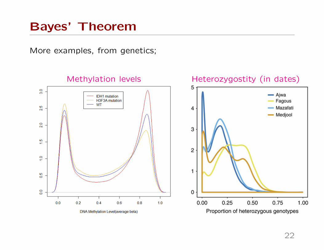
More examples, from genetics;

Methylation levels Heterozygostity (in dates)

22

Bayes’ Theorem

And one from XKCD;

23

Bayes’ Theorem

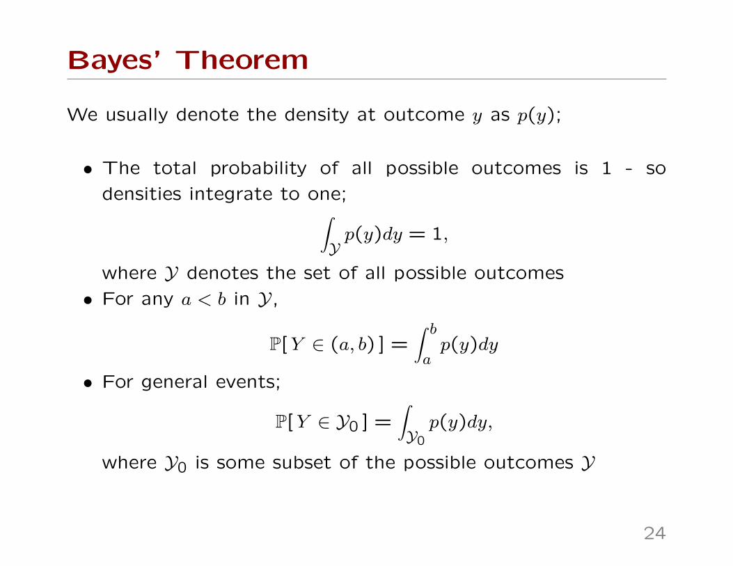
We usually denote the density at outcome y as p(y);

• The total probability of all possible outcomes is 1 - so

densities integrate to one;∫Yp(y)dy = 1,

where Y denotes the set of all possible outcomes

• For any a < b in Y,

P[Y ∈ (a, b) ] =∫ b

ap(y)dy

• For general events;

P[Y ∈ Y0 ] =∫Y0

p(y)dy,

where Y0 is some subset of the possible outcomes Y

24

Bayes’ Theorem

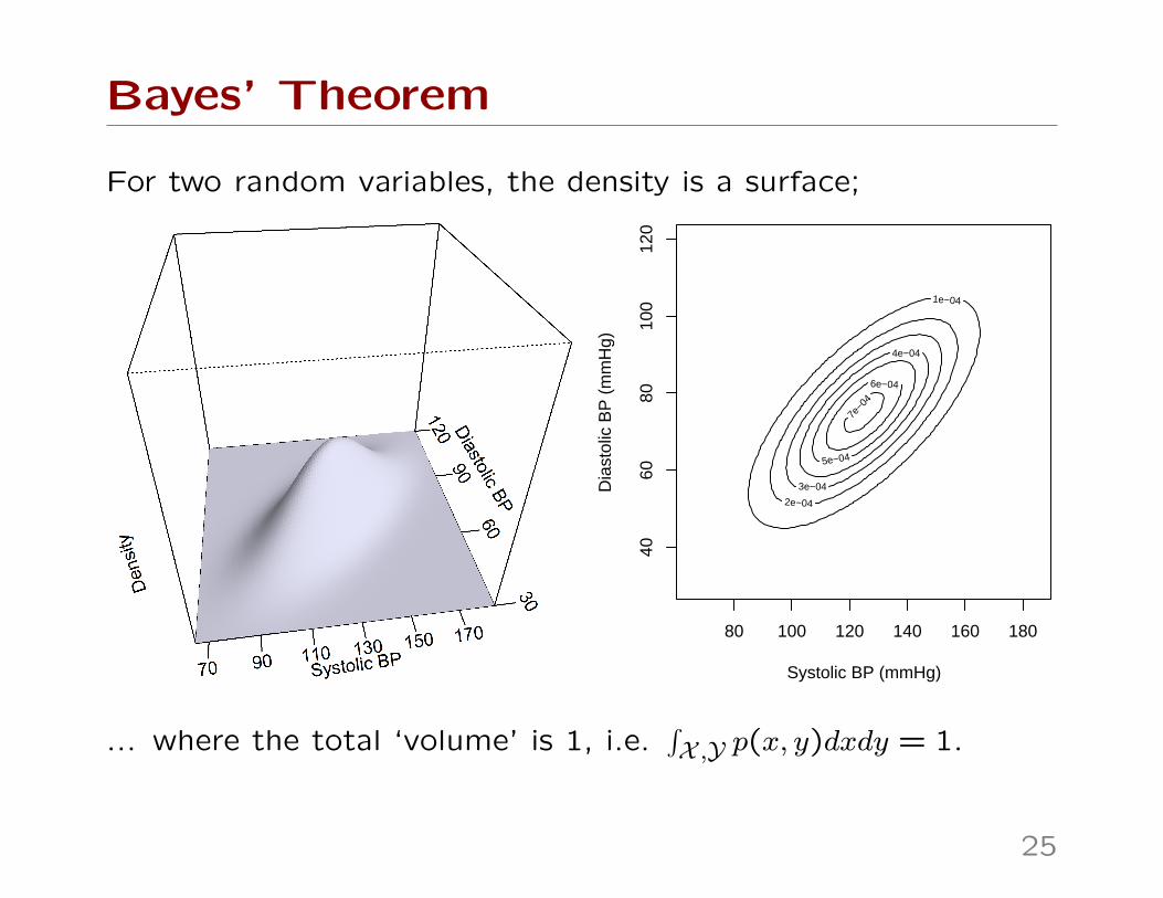
For two random variables, the density is a surface;

Systolic BP (mmHg)

Dia

stol

ic B

P (

mm

Hg)

1e−04

2e−04

3e−04

4e−04

5e−04

6e−04

7e−

04

80 100 120 140 160 18040

6080

100

120

... where the total ‘volume’ is 1, i.e.∫X ,Y p(x, y)dxdy = 1.

25

Bayes’ Theorem

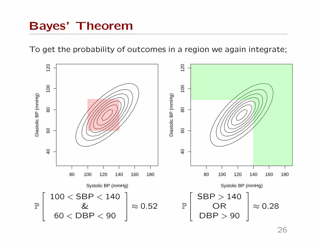
To get the probability of outcomes in a region we again integrate;

Systolic BP (mmHg)

Dia

stol

ic B

P (

mm

Hg)

80 100 120 140 160 180

4060

8010

012

0

Systolic BP (mmHg)

Dia

stol

ic B

P (

mm

Hg)

80 100 120 140 160 180

4060

8010

012

0

P

100 < SBP < 140&

60 < DBP < 90

≈ 0.52 P

SBP > 140OR

DBP > 90

≈ 0.28

26

Bayes’ Theorem

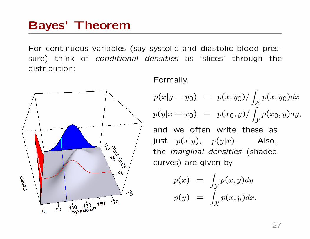
For continuous variables (say systolic and diastolic blood pres-sure) think of conditional densities as ‘slices’ through thedistribution;

Formally,

p(x|y = y0) = p(x, y0)/∫Xp(x, y0)dx

p(y|x = x0) = p(x0, y)/∫Yp(x0, y)dy,

and we often write these as

just p(x|y), p(y|x). Also,

the marginal densities (shaded

curves) are given by

p(x) =∫Yp(x, y)dy

p(y) =∫Xp(x, y)dx.

27

Bayes’ Theorem

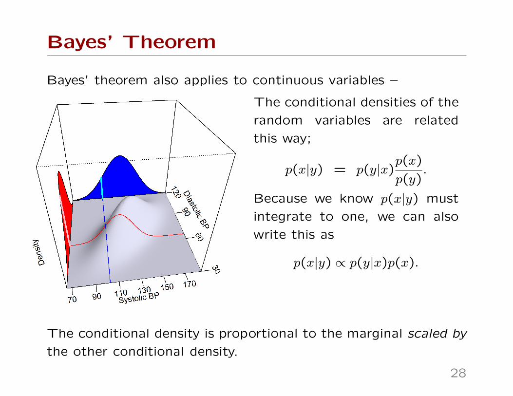
Bayes’ theorem also applies to continuous variables –

The conditional densities of the

random variables are related

this way;

p(x|y) = p(y|x)p(x)

p(y).

Because we know p(x|y) must

integrate to one, we can also

write this as

p(x|y) ∝ p(y|x)p(x).

The conditional density is proportional to the marginal scaled by

the other conditional density.

28

Bayesian statistics

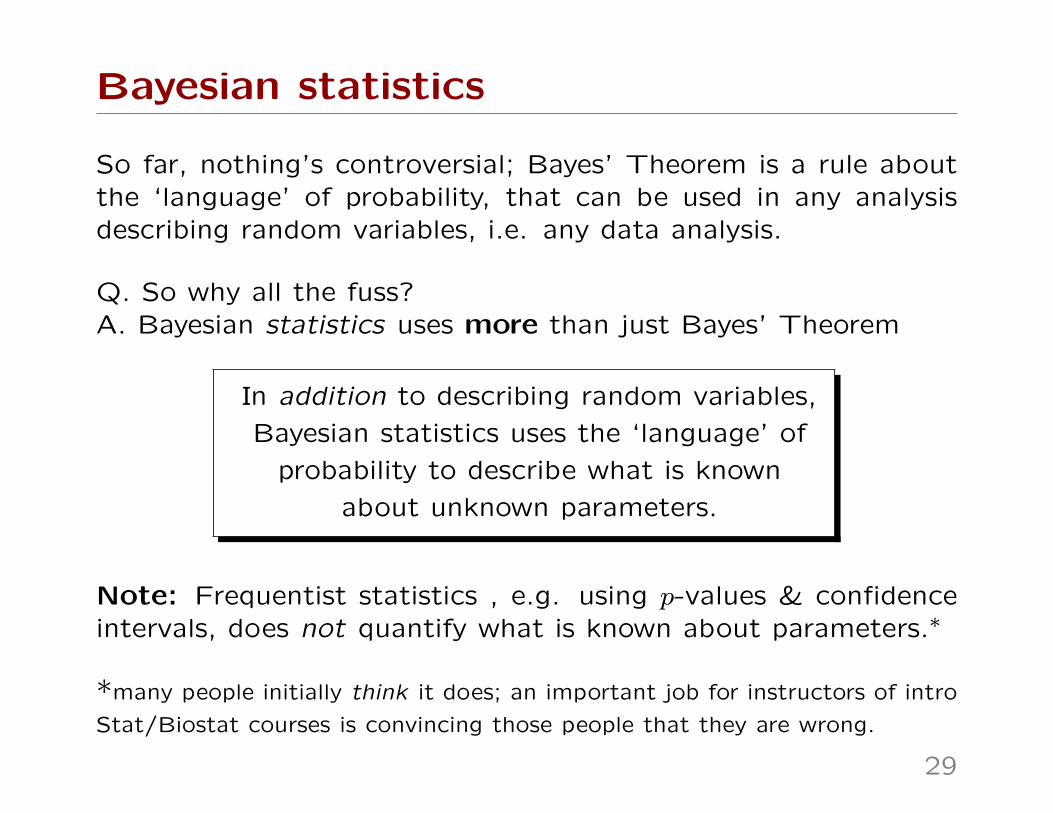
So far, nothing’s controversial; Bayes’ Theorem is a rule aboutthe ‘language’ of probability, that can be used in any analysisdescribing random variables, i.e. any data analysis.

Q. So why all the fuss?A. Bayesian statistics uses more than just Bayes’ Theorem

In addition to describing random variables,

Bayesian statistics uses the ‘language’ of

probability to describe what is known

about unknown parameters.

Note: Frequentist statistics , e.g. using p-values & confidenceintervals, does not quantify what is known about parameters.∗

*many people initially think it does; an important job for instructors of intro

Stat/Biostat courses is convincing those people that they are wrong.

29

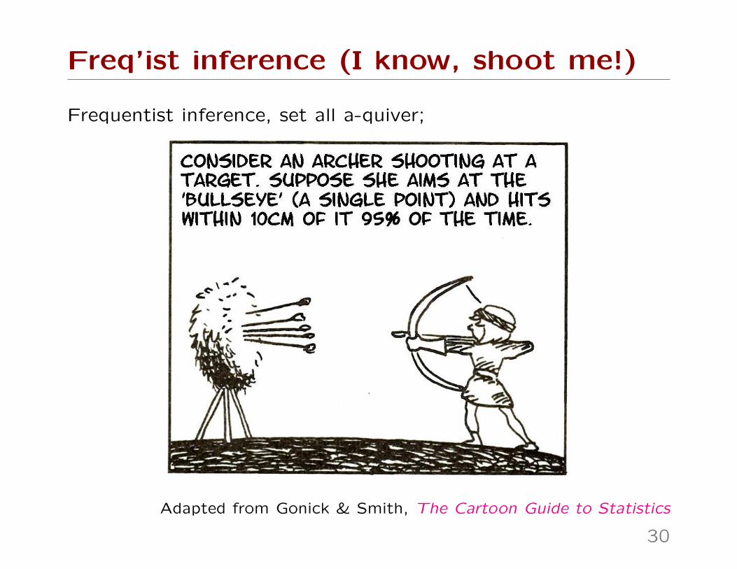
Freq’ist inference (I know, shoot me!)

Frequentist inference, set all a-quiver;

Adapted from Gonick & Smith, The Cartoon Guide to Statistics

30

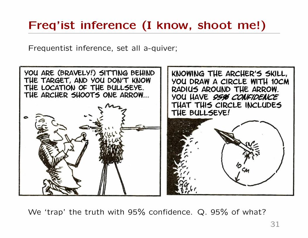
Freq’ist inference (I know, shoot me!)

Frequentist inference, set all a-quiver;

We ‘trap’ the truth with 95% confidence. Q. 95% of what?

31

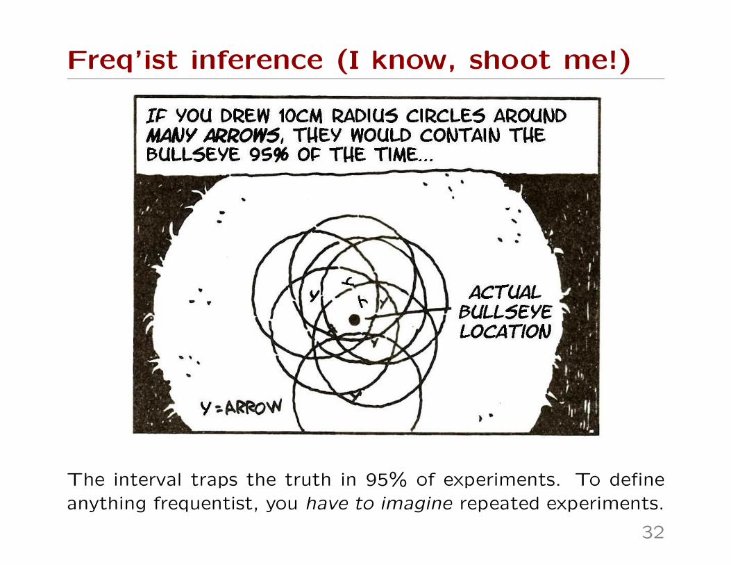
Freq’ist inference (I know, shoot me!)

The interval traps the truth in 95% of experiments. To defineanything frequentist, you have to imagine repeated experiments.

32

Freq’ist inference (I know, shoot me!)

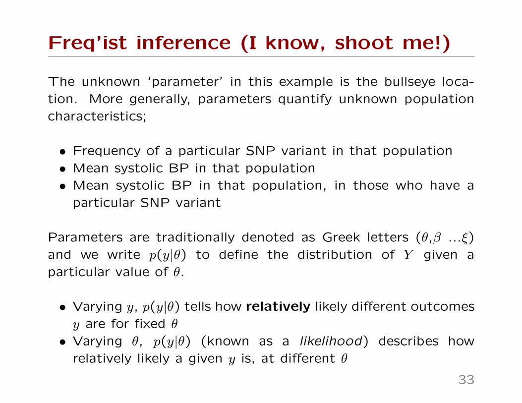
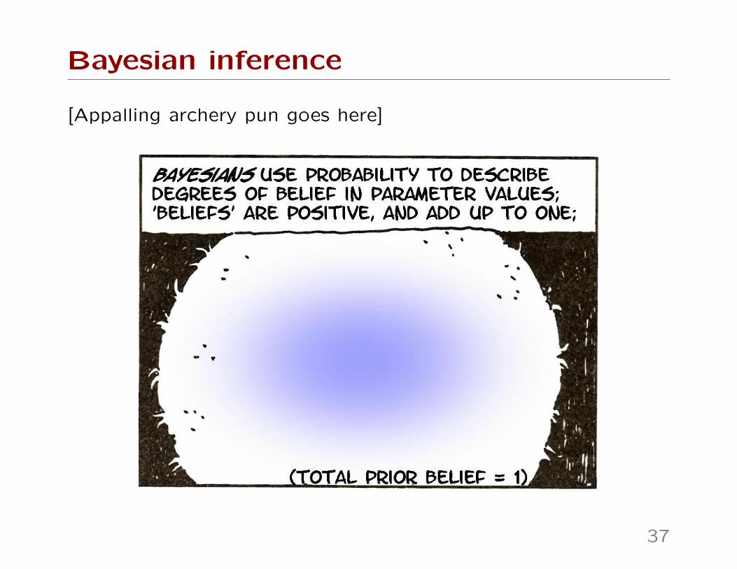
The unknown ‘parameter’ in this example is the bullseye loca-tion. More generally, parameters quantify unknown populationcharacteristics;

• Frequency of a particular SNP variant in that population• Mean systolic BP in that population• Mean systolic BP in that population, in those who have a

particular SNP variant

Parameters are traditionally denoted as Greek letters (θ,β ...ξ)and we write p(y|θ) to define the distribution of Y given aparticular value of θ.

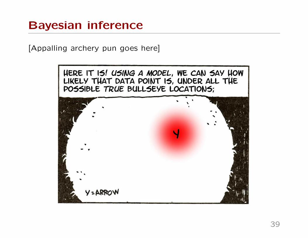
• Varying y, p(y|θ) tells how relatively likely different outcomesy are for fixed θ

• Varying θ, p(y|θ) (known as a likelihood) describes howrelatively likely a given y is, at different θ

33

Freq’ist inference (I know, shoot me!)

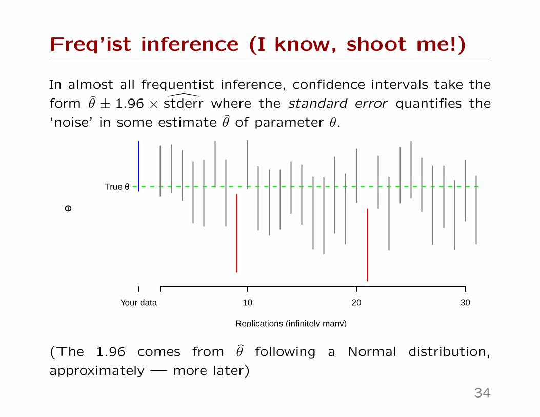
In almost all frequentist inference, confidence intervals take the

form θ ± 1.96 × stderr where the standard error quantifies the

‘noise’ in some estimate θ of parameter θ.

Replications (infinitely many)

ΘΘ

10 20 30Your data

True θθ

(The 1.96 comes from θ following a Normal distribution,

approximately — more later)

34

Freq’ist inference (I know, shoot me!)

Usually, we imagine running the ‘experiment’ again and again.Or, perhaps, make an argument like this;

On day 1 you collect data and construct a [valid] 95% confidenceinterval for a parameter θ1. On day 2 you collect new data andconstruct a 95% confidence interval for an unrelated parameterθ2. On day 3 ... [the same]. You continue this way constructingconfidence intervals for a sequence of unrelated parameters θ1, θ2,... 95% of your intervals will trap the true parameter value

Larry Wasserman, All of Statistics

This alternative interpretation is also valid, but...

• ... neither version says anything about whether your data isin the 95% or the 5%• ... both versions require you to think about many other

datasets, not just the one you have to analyze

How does Bayesian inference differ? Let’s take aim...

35

Bayesian inference

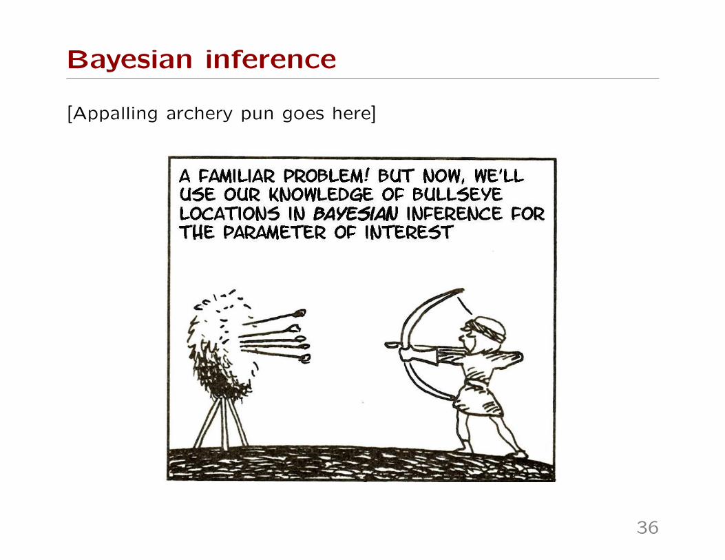
[Appalling archery pun goes here]

36

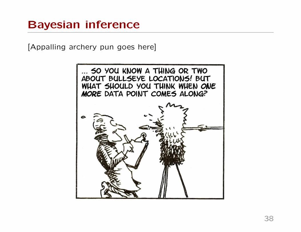
Bayesian inference

[Appalling archery pun goes here]

37

Bayesian inference

[Appalling archery pun goes here]

38

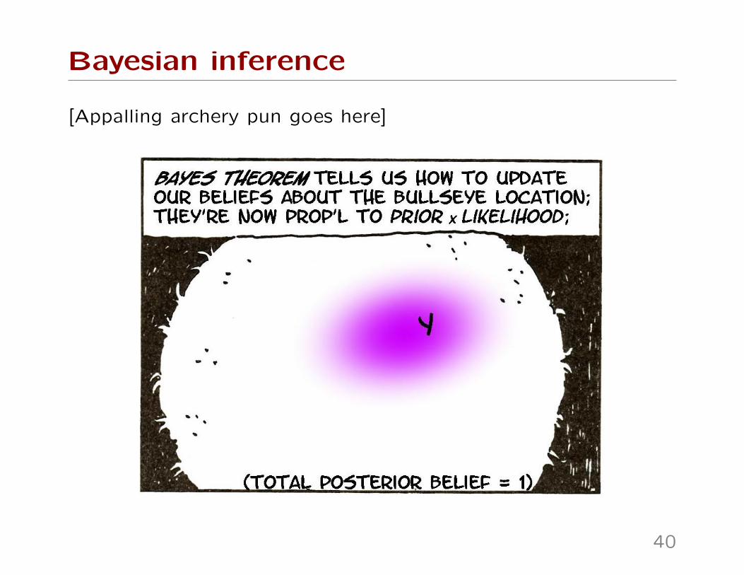
Bayesian inference

[Appalling archery pun goes here]

39

Bayesian inference

[Appalling archery pun goes here]

40

Bayesian inference

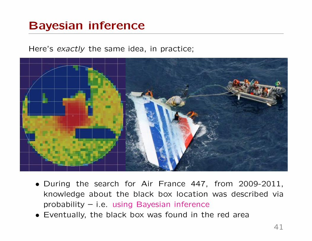
Here’s exactly the same idea, in practice;

• During the search for Air France 447, from 2009-2011,knowledge about the black box location was described viaprobability – i.e. using Bayesian inference• Eventually, the black box was found in the red area

41

Bayesian inference

How to update knowledge, as data is obtained? We use;

• Prior distribution: what you know about parameter θθθ,excluding the information in the data – denoted p(θθθ)• Likelihood: based on modeling assumptions, how (rela-

tively) likely the data y are if the truth is θθθ – denoted p(y|θθθ)

So how to get a posterior distribution: stating what we knowabout βββ, combining the prior with the data – denoted p(βββ|Y)?Bayes Theorem used for inference tells us to multiply;

p(θθθ|y) ∝ p(y|θθθ) × p(θθθ)

Posterior ∝ Likelihood × Prior.

... and that’s it! (essentially!)

• No replications – e.g. no replicate plane searches• Given modeling assumptions & prior, process is automatic• Keep adding data, and updating knowledge, as data becomes

available... knowledge will concentrate around true θθθ

42

Bayesian inference

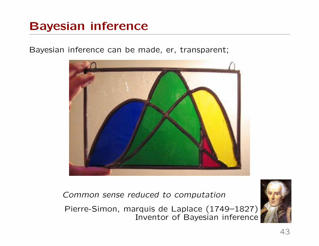
Bayesian inference can be made, er, transparent;

Common sense reduced to computation

Pierre-Simon, marquis de Laplace (1749–1827)Inventor of Bayesian inference

43

Bayesian inference

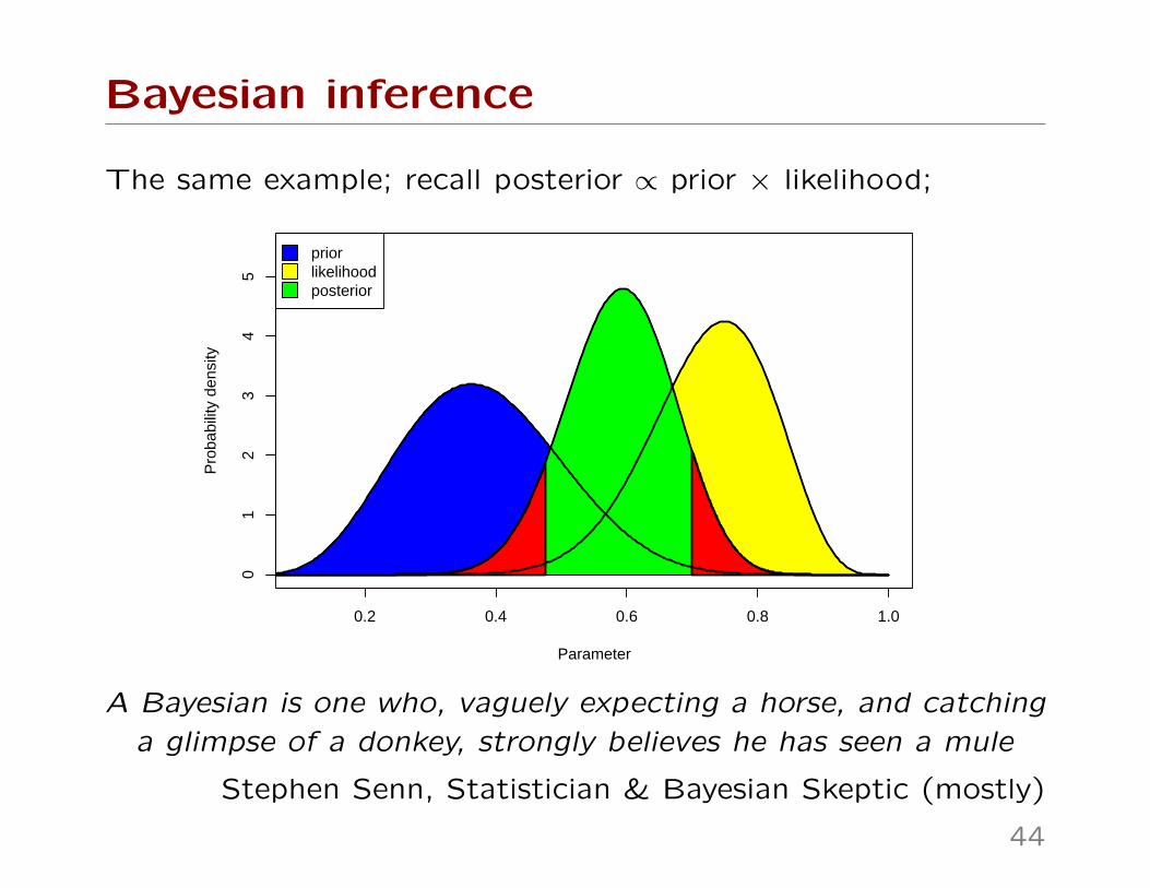
The same example; recall posterior ∝ prior × likelihood;

0.2 0.4 0.6 0.8 1.0

01

23

45

Parameter

Pro

babi

lity

dens

ity

priorlikelihoodposterior

A Bayesian is one who, vaguely expecting a horse, and catching

a glimpse of a donkey, strongly believes he has seen a mule

Stephen Senn, Statistician & Bayesian Skeptic (mostly)

44

But where do priors come from?

An important day at statistician-school?

There’s nothing wrong, dirty, unnatural or even unusual aboutmaking assumptions – carefully. Scientists & statisticians allmake assumptions... even if they don’t like to talk about them.

45

But where do priors come from?

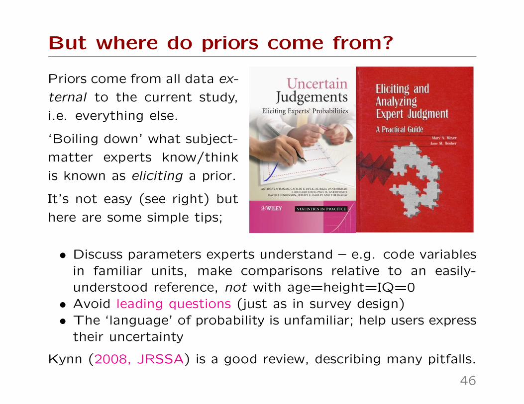
Priors come from all data ex-

ternal to the current study,

i.e. everything else.

‘Boiling down’ what subject-

matter experts know/think

is known as eliciting a prior.

It’s not easy (see right) but

here are some simple tips;

• Discuss parameters experts understand – e.g. code variablesin familiar units, make comparisons relative to an easily-understood reference, not with age=height=IQ=0• Avoid leading questions (just as in survey design)• The ‘language’ of probability is unfamiliar; help users express

their uncertainty

Kynn (2008, JRSSA) is a good review, describing many pitfalls.

46

But where do priors come from?

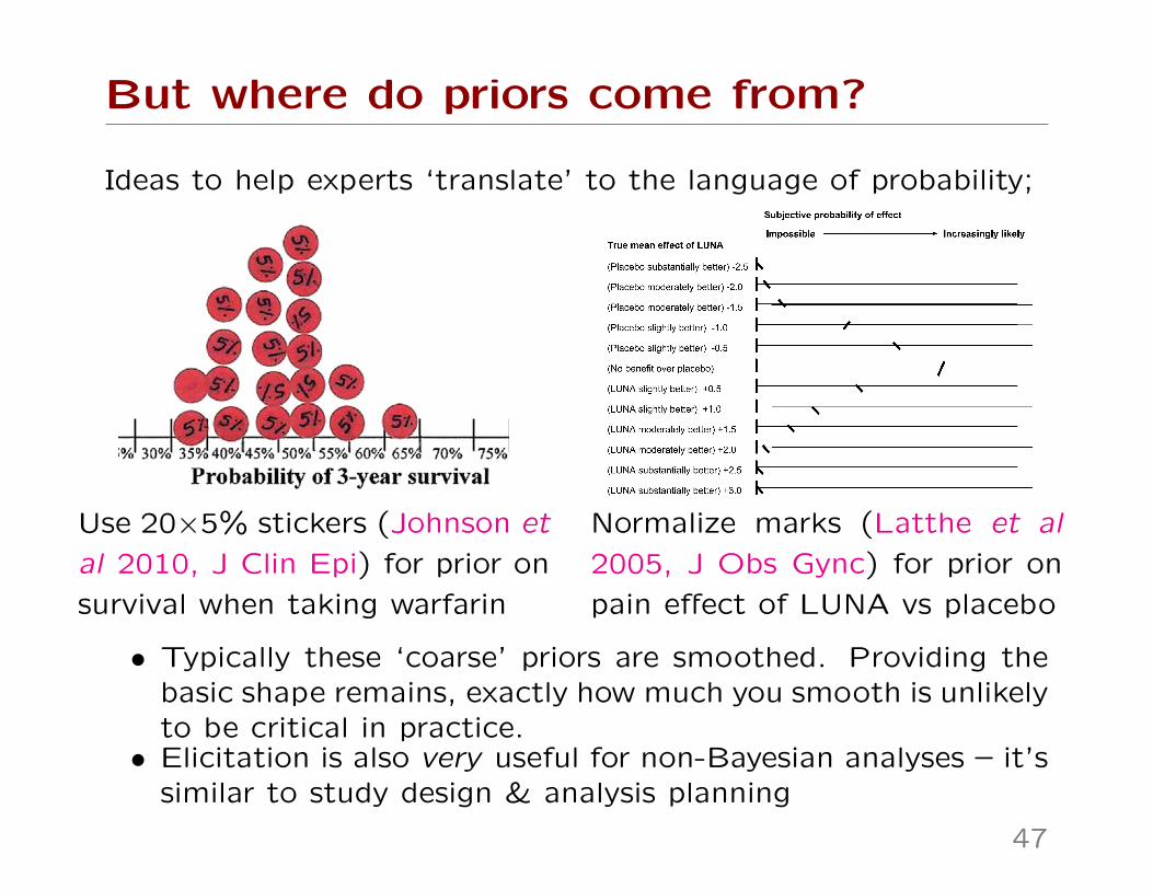
Ideas to help experts ‘translate’ to the language of probability;

Use 20×5% stickers (Johnson et

al 2010, J Clin Epi) for prior on

survival when taking warfarin

Normalize marks (Latthe et al

2005, J Obs Gync) for prior on

pain effect of LUNA vs placebo

• Typically these ‘coarse’ priors are smoothed. Providing thebasic shape remains, exactly how much you smooth is unlikelyto be critical in practice.• Elicitation is also very useful for non-Bayesian analyses – it’s

similar to study design & analysis planning

47

But where do priors come from?

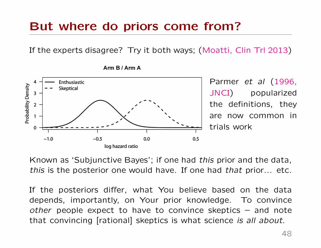
If the experts disagree? Try it both ways; (Moatti, Clin Trl 2013)

Parmer et al (1996,

JNCI) popularized

the definitions, they

are now common in

trials work

Known as ‘Subjunctive Bayes’; if one had this prior and the data,this is the posterior one would have. If one had that prior... etc.

If the posteriors differ, what You believe based on the datadepends, importantly, on Your prior knowledge. To convinceother people expect to have to convince skeptics – and notethat convincing [rational] skeptics is what science is all about.

48

When don’t priors matter (much)?

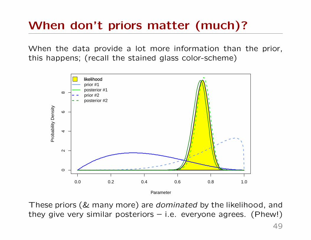
When the data provide a lot more information than the prior,this happens; (recall the stained glass color-scheme)

0.0 0.2 0.4 0.6 0.8 1.0

02

46

8

Parameter

Pro

babi

lity

Den

sity

prior #1posterior #1prior #2posterior #2

likelihood likelihood

These priors (& many more) are dominated by the likelihood, andthey give very similar posteriors – i.e. everyone agrees. (Phew!)

49

When don’t priors matter (much)?

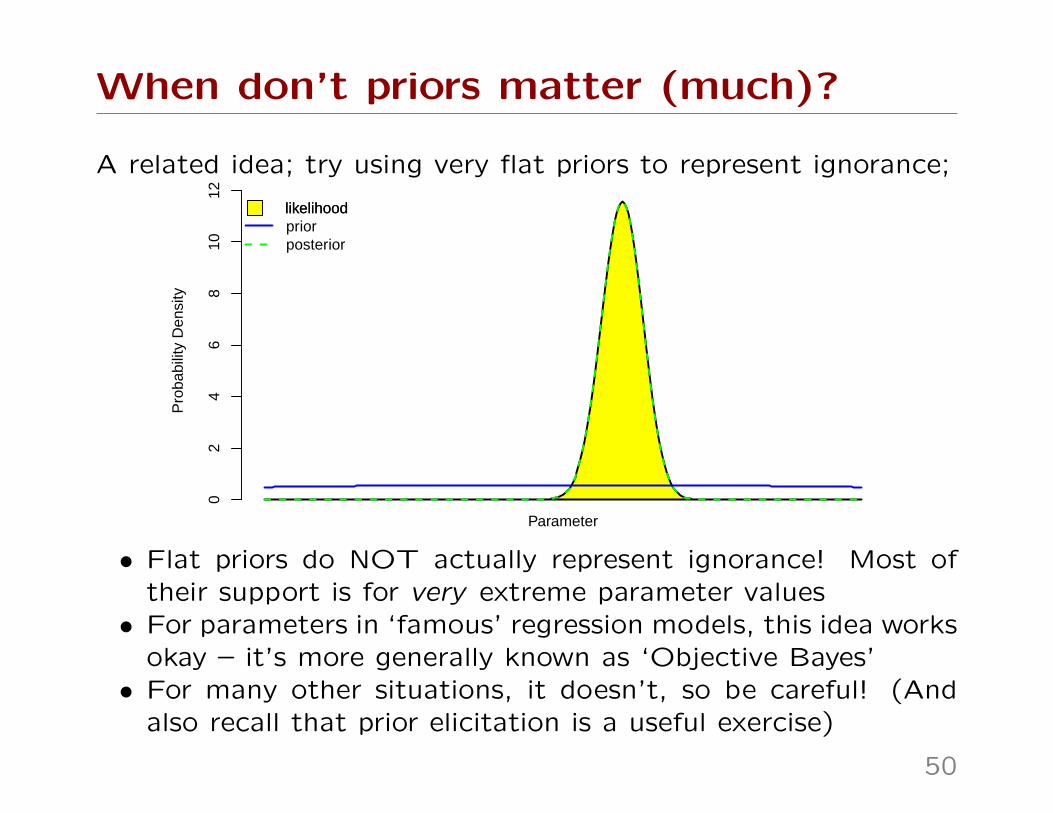
A related idea; try using very flat priors to represent ignorance;P

roba

bilit

y D

ensi

ty

02

46

810

12

Parameter

priorposterior

likelihood likelihood

• Flat priors do NOT actually represent ignorance! Most oftheir support is for very extreme parameter values• For parameters in ‘famous’ regression models, this idea works

okay – it’s more generally known as ‘Objective Bayes’• For many other situations, it doesn’t, so be careful! (And

also recall that prior elicitation is a useful exercise)

50

When don’t priors matter (much)?

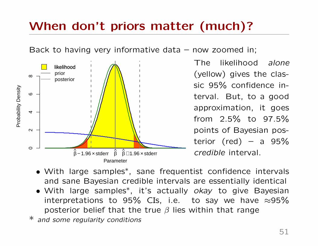
Back to having very informative data – now zoomed in;

Pro

babi

lity

Den

sity

02

46

8 priorposterior

likelihood likelihood

β − 1.96 × stderr β + 1.96 × stderrβParameter

The likelihood alone

(yellow) gives the clas-

sic 95% confidence in-

terval. But, to a good

approximation, it goes

from 2.5% to 97.5%

points of Bayesian pos-

terior (red) – a 95%

credible interval.

• With large samples∗, sane frequentist confidence intervalsand sane Bayesian credible intervals are essentially identical• With large samples∗, it’s actually okay to give Bayesian

interpretations to 95% CIs, i.e. to say we have ≈95%posterior belief that the true β lies within that range

* and some regularity conditions

51

When don’t priors matter (much)?

We can exploit this idea to be ‘semi-Bayesian’; multiply what

the likelihood-based interval says by Your prior.

One way to do this;

• Take point-estimate β and corresponding standard error

stderr, calculate precision 1/stderr2

• Elicit prior mean β0 and prior standard deviation σ; calculate

prior precision 1/σ2

• ‘Posterior’ precision = 1/stderr2 + 1/σ2 (which gives overall

uncertainty

• ‘Posterior’ mean = precision-weighted mean of β and β0

Note: This is a (very) quick-and-dirty approach; we’ll see much

more precise approaches in later sessions.

52

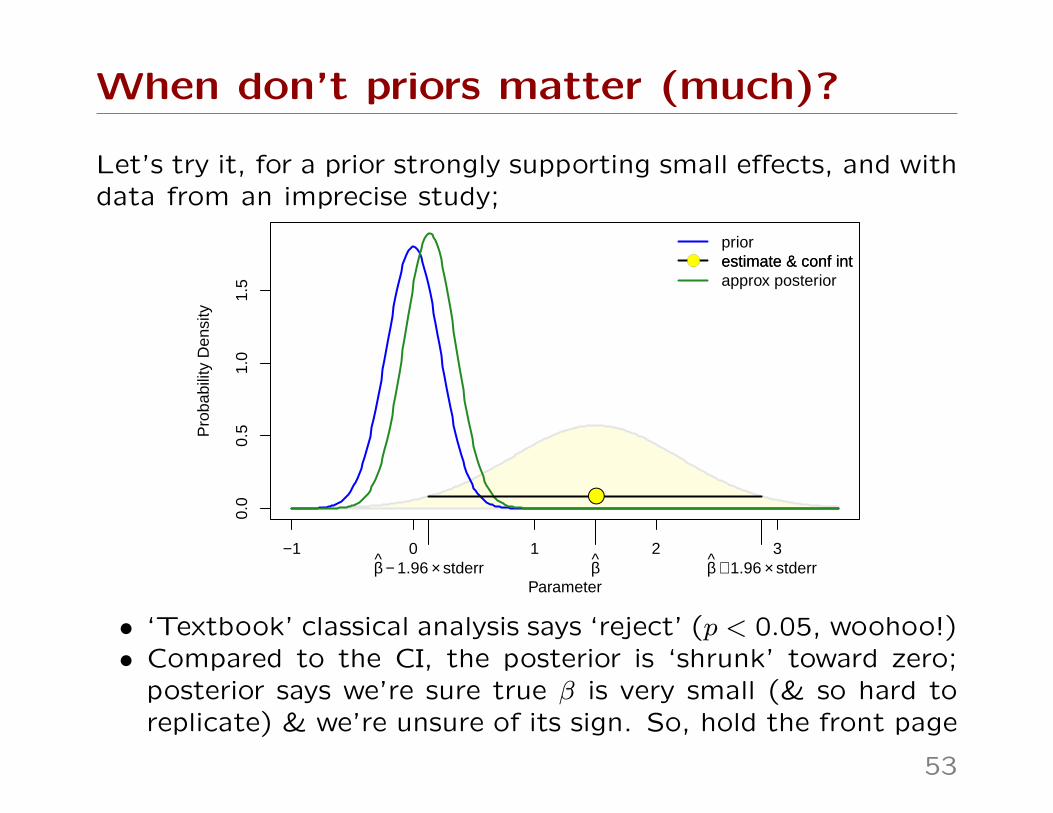
When don’t priors matter (much)?

Let’s try it, for a prior strongly supporting small effects, and withdata from an imprecise study;

−1 0 1 2 3

0.0

0.5

1.0

1.5

Parameter

Pro

babi

lity

Den

sity

●

β − 1.96 × stderr β + 1.96 × stderrβ

priorestimate & conf intapprox posterior

● estimate & conf int

• ‘Textbook’ classical analysis says ‘reject’ (p < 0.05, woohoo!)• Compared to the CI, the posterior is ‘shrunk’ toward zero;

posterior says we’re sure true β is very small (& so hard toreplicate) & we’re unsure of its sign. So, hold the front page

53

When don’t priors matter (much)?

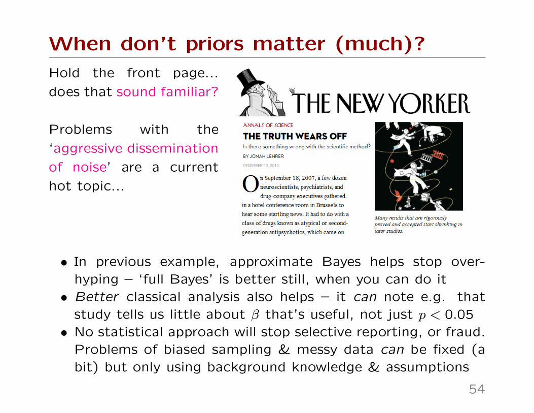
Hold the front page...

does that sound familiar?

Problems with the

‘aggressive dissemination

of noise’ are a current

hot topic...

• In previous example, approximate Bayes helps stop over-hyping – ‘full Bayes’ is better still, when you can do it• Better classical analysis also helps – it can note e.g. that

study tells us little about β that’s useful, not just p < 0.05• No statistical approach will stop selective reporting, or fraud.

Problems of biased sampling & messy data can be fixed (abit) but only using background knowledge & assumptions

54

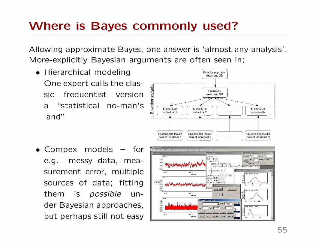
Where is Bayes commonly used?

Allowing approximate Bayes, one answer is ‘almost any analysis’.More-explicitly Bayesian arguments are often seen in;

• Hierarchical modeling

One expert calls the clas-

sic frequentist version

a “statistical no-man’s

land”

• Compex models – for

e.g. messy data, mea-

surement error, multiple

sources of data; fitting

them is possible un-

der Bayesian approaches,

but perhaps still not easy

55

Are all classical methods Bayesian?

We’ve seen that, for popular regression methods, with large n,Bayesian and frequentist ideas often don’t disagree much. Thisis (provably!) true more broadly, though for some situationsstatisticians haven’t yet figured out the details. Some ‘fancy’frequentist methods that can be viewed as Bayesian are;

• Fisher’s exact test – its p-value is the ‘tail area’ of theposterior under a rather conservative prior (Altham 1969)• Conditional logistic regression – like Bayesian analysis with

particular random effects models (Severini 1999, Rice 2004)• Robust standard errors – like Bayesian analysis of a ‘trend’,

at least for linear regression (Szpiro et al 2010)

And some that can’t;

• Many high-dimensional problems (shrinkage, machine-learning)• Hypothesis testing (‘Jeffrey’s paradox’) ...but NOT signifi-

cance testing (Rice 2010... available as a talk)

And while e.g. hierarchical modeling & multiple imputation areeasier to justify in Bayesian terms, they aren’t unfrequentist.

56

Fight! Fight! Fight!

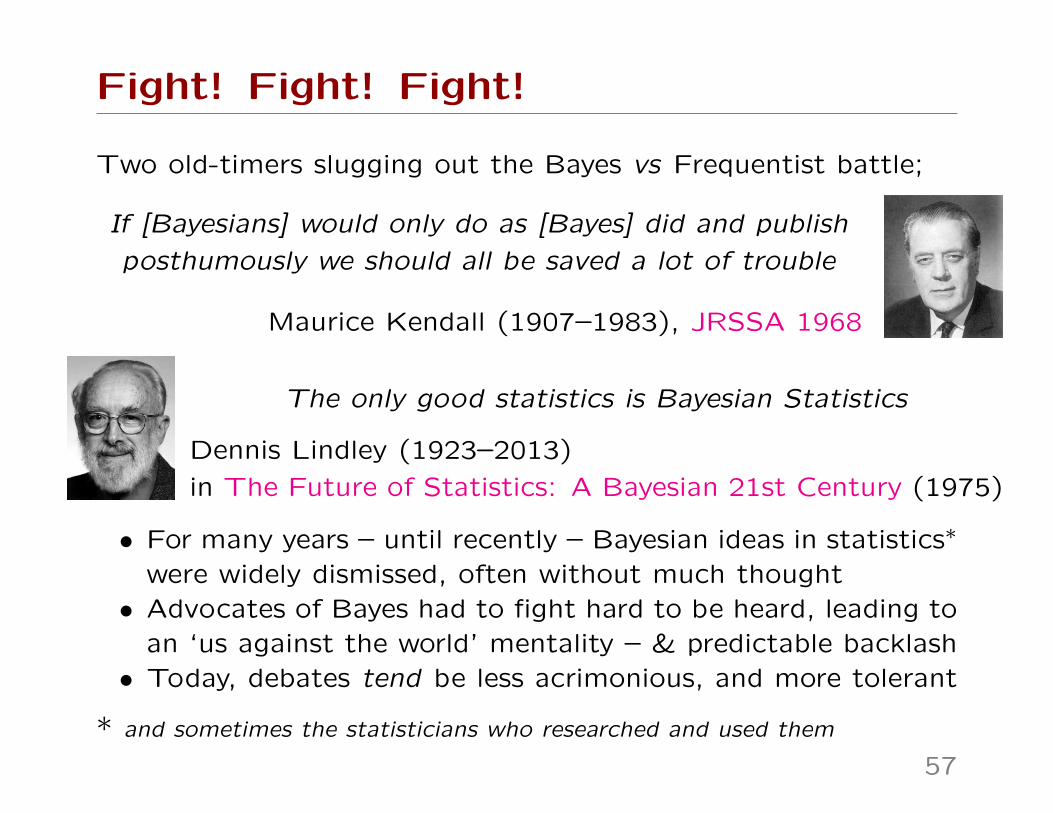
Two old-timers slugging out the Bayes vs Frequentist battle;

If [Bayesians] would only do as [Bayes] did and publish

posthumously we should all be saved a lot of trouble

Maurice Kendall (1907–1983), JRSSA 1968

The only good statistics is Bayesian Statistics

Dennis Lindley (1923–2013)

in The Future of Statistics: A Bayesian 21st Century (1975)

• For many years – until recently – Bayesian ideas in statistics∗

were widely dismissed, often without much thought• Advocates of Bayes had to fight hard to be heard, leading to

an ‘us against the world’ mentality – & predictable backlash• Today, debates tend be less acrimonious, and more tolerant

* and sometimes the statisticians who researched and used them

57

Fight! Fight! Fight!

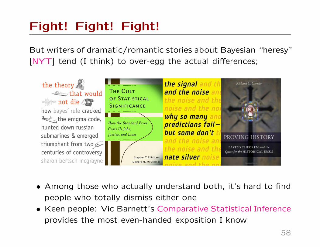
But writers of dramatic/romantic stories about Bayesian “heresy”

[NYT] tend (I think) to over-egg the actual differences;

• Among those who actually understand both, it’s hard to find

people who totally dismiss either one

• Keen people: Vic Barnett’s Comparative Statistical Inference

provides the most even-handed exposition I know

58

Fight! Fight! Fight!

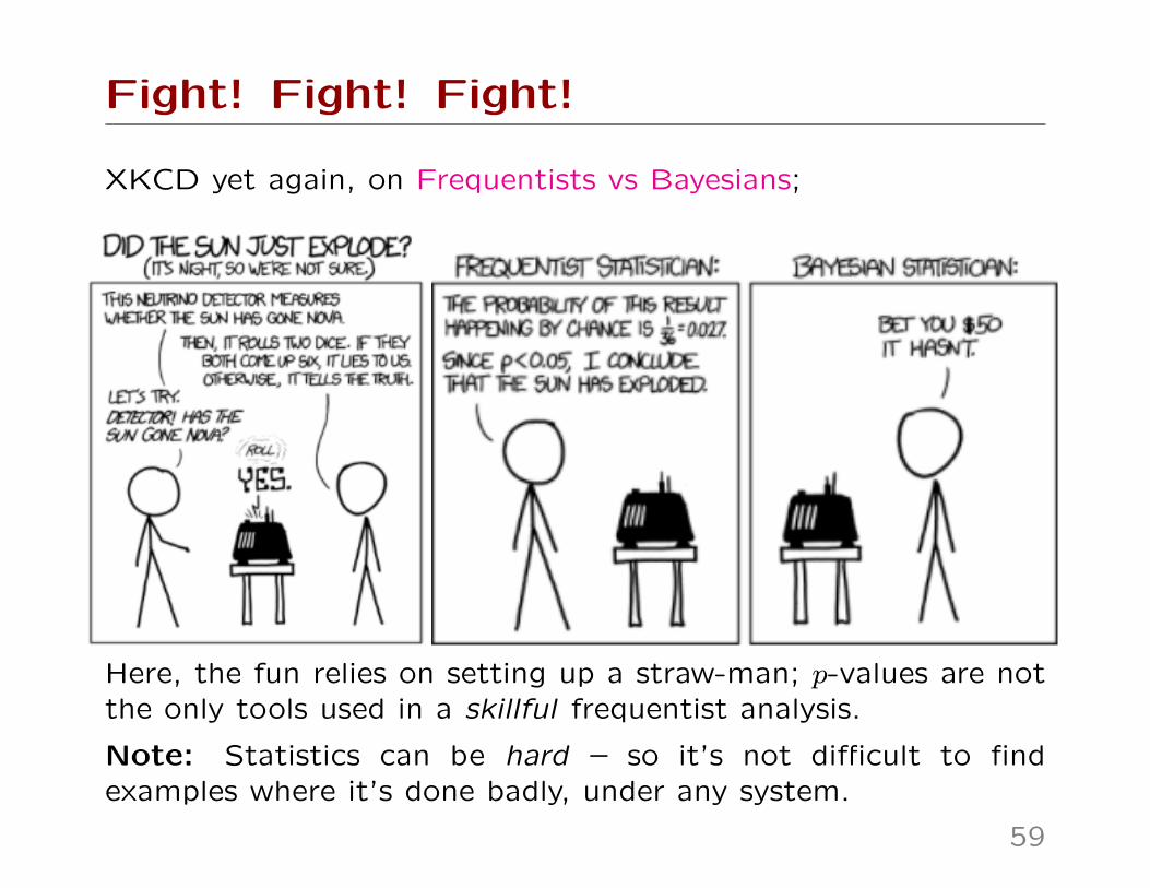
XKCD yet again, on Frequentists vs Bayesians;

Here, the fun relies on setting up a straw-man; p-values are notthe only tools used in a skillful frequentist analysis.

Note: Statistics can be hard – so it’s not difficult to findexamples where it’s done badly, under any system.

59

What did you miss out?

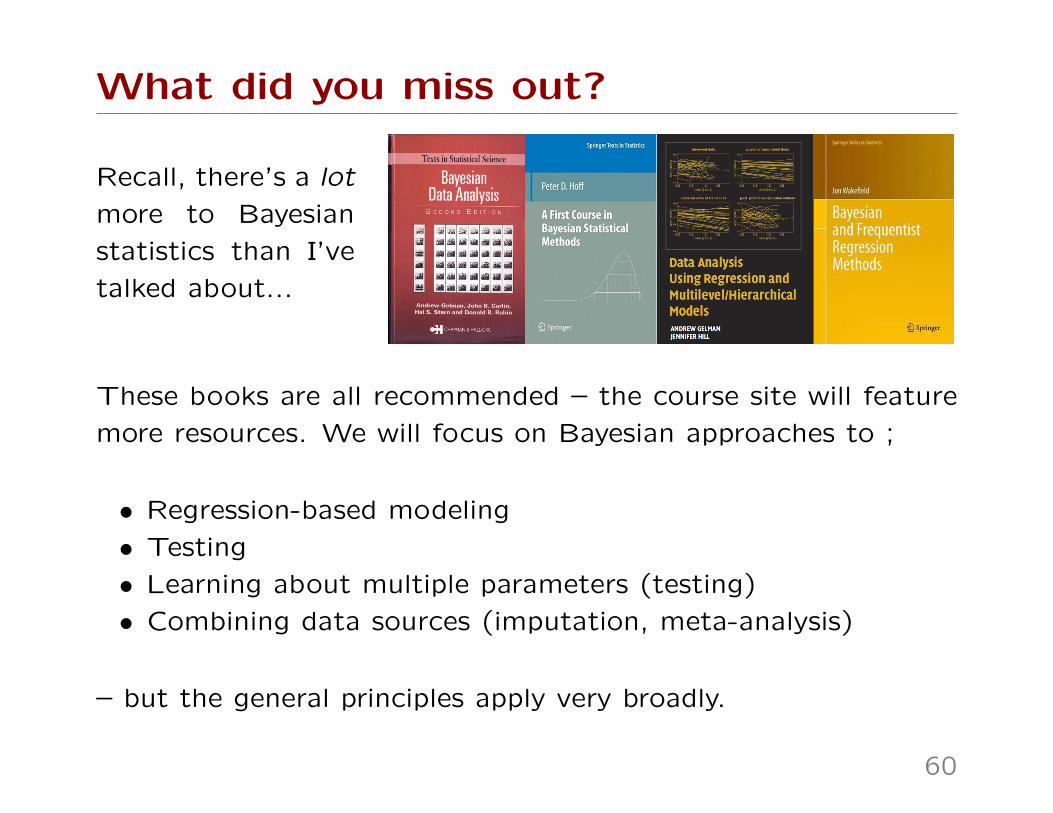
Recall, there’s a lot

more to Bayesian

statistics than I’ve

talked about...

These books are all recommended – the course site will feature

more resources. We will focus on Bayesian approaches to ;

• Regression-based modeling

• Testing

• Learning about multiple parameters (testing)

• Combining data sources (imputation, meta-analysis)

– but the general principles apply very broadly.

60

Summary

Bayesian statistics:

• Is useful in many settings, and intuitive

• Is often not very different in practice from frequentist

statistics; it is often helpful to think about analyses from

both Bayesian and non-Bayesian points of view

• Is not reserved for hard-core mathematicians, or computer

scientists, or philosophers. Practical uses abound.

Wikipedia’s Bayes pages aren’t great. Instead, start with the

linked texts, or these;

• Scholarpedia entry on Bayesian statistics

• Peter Hoff’s book on Bayesian methods

• The Handbook of Probability’s chapter on Bayesian statistics

• Ken’s website, or Jon’s website

61