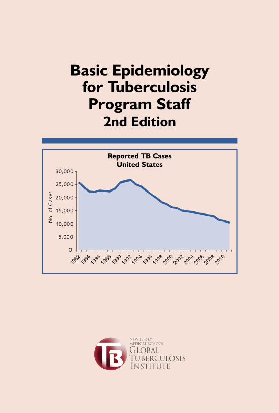
Basic Epidemiology for Tuberculosis Program Staff 2nd Edition Reported TB Cases United States 0 5,000 10,000 15,000 20,000 25,000 30,000 No. of Cases

Welcome message from author
This document is posted to help you gain knowledge. Please leave a comment to let me know what you think about it! Share it to your friends and learn new things together.
Transcript
Basic Epidemiology for Tuberculosis
Program Staff2nd Edition
Reported TB CasesUnited States
0
5,000
10,000
15,000
20,000
25,000
30,000
No.
of
Cas
es

Basic Epidemiology for Tuberculosis Program Staff
2nd Edition
Marian Passannante, PhDAssociate Professor, New Jersey Medical School & School of Public Health
Epidemiologist, New Jersey Medical School Global TB InstituteUniversity of Medicine and Dentistry of New Jersey
Newark, New Jersey
Anna Sevilla, MPH, MBSResearch Coordinator
New Jersey Medical School Global TB InstituteUniversity of Medicine and Dentistry of New Jersey
Newark, New Jersey
Nisha Ahamed, MPHProgram Director, Education and Training
New Jersey Medical School Global TB InstituteUniversity of Medicine and Dentistry of New Jersey
Newark, New Jersey
This product is funded by the Centers for Disease Control and Prevention, Division of Tuberculosis Elimination
i
ii
AcknowledgmentsWe wish to thank the following individuals and groups who participated in
drafting and reviewing this guide:
Kathryn Arden, MD, MHASouth Carolina Dept. of Health and Environmental Control
Rajita Bhavaraju, MPH, CHES Eileen Napolitano, BA Lillian Pirog, RN, PNP Mark Wolman, MA, MPHNJMS-Global Tuberculosis Institute
Jennifer Grinsdale, MPHSan Francisco Dept. of Public Health
Nancy Baruch, RN, MBA Anna Lee, BSMaryland Dept. of Health and Mental Hygiene
Jason Cummins, MPH Trudy Stein-Hart, MS Tennessee Department of Health
Michele Dincher, RN, BSN Lisa Paulos, RN, MPHPennsylvania Dept. of Health
Nicole Evert, MS Patricia Thickstun, PhD Ann Tyree, MSTexas Dept. of State Health Services
Ellen Hill, MS, DLSHTMIdaho Dept. of Health and Welfare
Ann Hinds, BS, RNJohnson County Health System, Kansas
Mary McKenzie, EdM, MS, RNCity of Chelsea, Massachusetts Health Dept.
Roque Miramontes, PA-C, MPH Lori Armstrong, PhD Juliana Grant, MD, MPH Maryam Haddad, MSN, MPH Kai Young, MPHDivision of Tuberculosis Elimination Centers for Disease Control and Prevention
Darlene Morse, RN, MEd, CHES, CICNew Hampshire Dept. of Health and Human Services
Eyal Orel, MS, PhDSeattle & King County Public Health TB Control Program
Kristina Schaller, BSArizona Dept. of Health Services
Mary Katie Sisk, RN, CICDistrict of Columbia Dept. of Health
Sarah Solarz, BA, MPHMinnesota Department of Health
iii
Previous Edition – 2005
ReviewersDonna Allis, PhD, RN
Joanne Becker
Rajita Bhavaraju, MPH, CHES
Beverly Ann Collins, RN, MS, CIC
Denise Cory
Myrene Couves
Pete Denkowski
Patsy Eddington
Kim Field, RN, MSN
Vipra Ghimire, MPH, CHES
Chris Hayden, BA
Bart Holland, PhD, MPH
Natalia Kurepina, PhD
Kayla Laserson, ScD
Diane McCracken, RN
Eileen Napolitano, BA
Stephanie Napolitano, MPH
Thomas Navin, MD
Margaret Osborn, RN, BSN
Bob Parker, MS
Thomas Privett
Nandini Selvam, PhD, MPH
Mary Spinner, RN, BSN
Marie Villa, RN
Linda Weldon, RN, BSN
Diane Werling
Mark Wolman, MA, MPH
Oralia Zamora, RN
Prepared by: Marian Passannante, PhD, and Nisha Ahamed, MPH, CHES
All material in this document is in the public domain, except where noted “Reprinted here with permission.” All material in the public domain may be used and reprinted without special permission; citation of source, however, is appreciated.
Suggested citation: New Jersey Medical School Global Tuberculosis Institute. Basic Epidemiology for Tuberculosis Program Staff, 2nd Edition. 2012: (inclusive pages)
The New Jersey Medical School Global Tuberculosis Institute is a TB Regional Training and Medical Consultation Center (RTMCC) funded by the Centers for Disease Control and Prevention, Division of Tuberculosis Elimination.
Graphic Design: DeeDee Hamm

iv
v
Table of ContentsPart One: The Basics
1. Introduction – Uses of Epidemiology in Tuberculosis Control ............................................................................................ 1
2. What Is Epidemiology? ................................................................... 33. Types of Epidemiology .................................................................... 4
A. Descriptive Epidemiology ......................................................4i. Public Health Surveillance ......................................................4ii. Descriptive Epidemiology Using TB Surveillance Data ............6iii. Using TB Surveillance Data for Program Evaluation ...............9iv Accessing Data Online ........................................................11
B. Analytic Epidemiology ..........................................................124. Key Concepts in Epidemiology ..................................................... 13
A. Morbidity .............................................................................13i. Incidence ............................................................................14ii. Prevalence ..........................................................................16iii. Comparison of Incidence and Prevalence .............................17iv. Sample Calculations: Incidence and Prevalence ...................19
B. Mortality ..............................................................................21i. Measures of Mortality .........................................................21ii. Sample Calculation of Crude and Age-Specific Mortality
Rates ...................................................................................22iii. Age-Adjusted Rates ............................................................24iv. Case-Fatality Rate ...............................................................26v. Cause-Specific Mortality Rate ..............................................29
5. Presenting TB Program Data ...................................................... 32A. Measurement Scales .............................................................32B. Summarizing the Data ..........................................................32
i. The Middle Values...............................................................33ii. Variation .............................................................................34iii. Which Measures to Use? .....................................................37
C. Presenting Data ....................................................................39i. Bar Charts or Graphs and Pie Charts ....................................39ii. Histograms ..........................................................................42
vi
Part Two: Beyond the Basics6. Measuring Test Validity ................................................................ 46
A. Sensitivity, Specificity and Predictive Values .........................46B. Test Validity Examples ..........................................................48
7. Study Designs ............................................................................... 53A. Cross-Sectional Studies ........................................................53B. Case-Control Studies ............................................................54
i. Odds Ratios ........................................................................55ii. Sample Calculation: Odds Ratio ..........................................55
C. Cohort Studies .....................................................................56i. Relative Risk ........................................................................57ii. Sample Calculation: Relative Risk ........................................59
D. Clinical Trials .........................................................................608. Statistical Concepts Used in Epidemiologic Studies ................... 63
A. P-Values ................................................................................63B. Confidence Intervals .............................................................64C. Confounding Factors ............................................................66D. Bias ......................................................................................67E. Meta-analysis .......................................................................68
9. Molecular Epidemiology: Genotyping and TB Control ............... 70A. What Is TB Genotyping? .......................................................70B. National TB Genotyping Service and the TB
Genotyping Information Management System .....................71C. Using TB Genotyping in TB Outbreak Detection ...................72D. Cluster Investigations ...........................................................73
Part Three: Putting It All Together10. TB Case Study .............................................................................. 75
A. How to Use TB Surveillance Data in TB Control ....................75B. How to Use TB Surveillance Data in TB Control
Answer Key ..........................................................................83Appendix I – Common Statistical Terms Used in Epidemiology .... 87Appendix II – RVCT Form: Report of Verified Case of Tuberculosis .................................................................................... 101Appendix III – National TB Program Objectives .......................... 107Appendix IV – National Tuberculosis Indicators Project (NTIP) ............................................................................................. 111Appendix V – Solutions for Sample Problems .............................. 115Appendix VI – Suggested Reading List .......................................... 117
1
Part One: The Basics
Introduction – Uses of Epidemiology in 1. Tuberculosis ControlPrevention and control of tuberculosis (TB) in the United States is an important public health responsibility. Effective TB prevention and control requires a complex system that merges elements of laboratory science, investigative work, public health, surveillance, and clinical care. Epidemiology is the basic science of public health and provides a variety of tools that can be used in TB prevention and control activities.
An understanding of epidemiology is useful for all TB program staff, ranging from disease investigators and health care workers to TB program managers. The epidemiologic concepts presented in this guide will assist in analyzing and making practical use of data, assessing current and evolving trends in TB morbidity, identifying risk groups, and determining where to allocate staff and resources. Although not all TB program staff members are involved with all these activities, a broad understanding of epidemiologic principles can assist all TB program staff in working toward effective TB prevention and control.
This guide defines and describes key concepts and terminology in epidemiology and provides detailed examples and sample problems. Wherever possible, data and examples are drawn from existing epidemiologic studies related to TB. Most examples are from US populations. The guide presents descriptions of how these concepts can be put to practical use by TB program staff. It is not intended to be a complete text on TB or epidemiology, but rather a reference that can be used to learn or review key concepts of epidemiology that will be useful in the overall effort to prevent and control TB in the United States. This guide is intended for use by individuals in a broad variety of TB prevention and control positions, with a variety of job responsibilities.
The first section of this guide (Part One: Chapters 2 through 5) provides a basic background and understanding of epidemiology for TB program staff, focusing on specific uses of epidemiology to assess and implement TB programs. The second section of the guide (Part Two: Chapters 6 through 9) presents more advanced
2
concepts such as epidemiologic and statistical techniques that are used in research studies as well as a chapter on how genotyping is used in TB prevention and control. This information will assist TB program staff in reading and understanding TB-related articles in medical and public health journals. Awareness of new information about the epidemiology of TB and new research in TB transmission, diagnostics, and treatment can be very useful to TB program staff members who work to prevent and control TB within their program area. Part Three (Chapter 10) provides an exercise with an example of how data can help TB prevention and control staff identify trends and make decisions about the allocation of resources. An answer key is also provided.
Definitions of selected epidemiologic and statistical terms (in blue and underlined in the text) appear in Appendix I. In the online version of the guide, these terms are hyperlinked to the definitions in Appendix I. These definitions are from CDC’s EXCITE Glossary of Epidemiologic Terms http://www.cdc.gov/excite/library/glossary.htm
Original Source: Principles of Epidemiology in Public Health Practice, 3rd Edition. Developed by: U.S. Department of Health and Human Services, Centers for Disease Control and Prevention, Office of Workforce and Career Development, Career Development Division, Atlanta, GA 30333
3
What Is Epidemiology?2. Definitions of epidemiology vary, but the one used in this guide is presented below:
EpidemiologyThe study of the distribution and determinants of health conditions or events among populations and the application of that study to control health problems
Source: http://www.cdc.gov/excite/library/glossary.htm
A health condition or event should be thought of in a very broad context, including the occurrence of infection, symptomatic disease, injury, disability (which are all aspects of morbidity or illness) and even death or mortality. Epidemiology is a discipline that helps explore and understand patterns of morbidity and mortality within and between populations, using statistical methods to clarify these patterns. Understanding how diseases are distributed in a population and the factors that determine who gets the disease can help to identify ways to prevent and control its spread.
4
Types of Epidemiology3. Epidemiology is usually classified as descriptive or analytic.
EpidemiologyDescriptive epidemiology: The aspect of epidemiology concerned with organizing and summarizing data regarding the persons affected (e.g., the characteristics of those who became ill), time (e.g., when they become ill), and place (e.g., where they might have been exposed to the cause of illness)
Analytic epidemiology: The aspect of epidemiology concerned with why and how a health problem occurs. Analytic epidemiology uses comparison groups to provide baseline or expected values so that associations between exposures and outcomes can be quantified and hypotheses about the cause of the problem can be tested
Source: http://www.cdc.gov/excite/library/glossary.htm
Descriptive epidemiology describes who (person), where (place), and when (time) a disease (what) occurs. Analytic epidemiology looks for why and how diseases are spread. Another way to think about descriptive epidemiology versus analytic epidemiology involves hypotheses, or tentative explanations for observations or scientific problems. Hypotheses are generated through descriptive epidemiology, whereas analytic epidemiology allows testing of those hypotheses to determine if they are likely to be correct or incorrect.
A. Descriptive Epidemiologyi. Public Health SurveillanceDescriptive epidemiologic data related to TB are collected through public health surveillance activities.
Public Health SurveillancePublic health surveillance is the ongoing, systematic collection, analysis, and interpretation of health data, essential to the planning, implementation and evaluation of public health practice, closely integrated with the dissemination of these data to those who need to know and linked to prevention and control.
Source: Thacker SB, Berkelman RL. History of public health surveillance In: Public Health Surveillance, Halperin W, Baker EL (Eds.): New York; Van Norstrand Reinhold, 1992.
5
The purpose of public health surveillance is to gain knowledge of the patterns of disease, injury, and other health problems in a community and thereby work toward controlling and preventing them.
Two types of public health surveillance are active and passive surveillance: active surveillance is a system in which the health department or other agency initiates the data collection activities. In TB prevention and control, testing (tuberculin skin test [TST] or interferon-γ release assays [IGRA]) by a health department among certain populations, such as persons living with HIV/AIDS, is an example of active surveillance for TB infection. In passive surveillance, the health department receives reports from the health care provider. For example, the CDC system for receiving reports of adverse effects associated with treatment is classified as passive surveillance.
Public health surveillance is an important part of an information feedback loop that links the public, health care providers, and health agencies.
Disease data that are collected through both active and passive surveillance mechanisms should be summarized by the official health agency and then sent back to those who can make use of this information at the provider or program level. These data can be useful for program evaluation and for developing health education programs, public health interventions, and public health recommendations that should then be disseminated to the general public. TB surveillance in the United States relies on both passive and active surveillance activities.
In the United States, requirements for reporting diseases are mandated by state laws or regulations. When such a law or regulation exists, health care providers, laboratories, and public health personnel report the occurrence of these notifiable diseases to state and local health departments. State health departments agree to report cases of selected diseases to CDC as a result of a policy established by CDC and the Council of State and Territorial Epidemiologists (CSTE). Active tuberculosis is one disease that must be reported to state health departments. Cases of TB are reported to CDC as a result of a cooperative agreement between CDC and the state or local
6
health department. Some state and local health departments require the collection of additional information; for example, some jurisdictions require the reporting of latent TB infection.
CDC has been collecting information on new cases of TB disease in the United States since 1953. Data on TB cases are collected using the Report of Verified Cases of Tuberculosis (RVCT) form (see Appendix II, page 101) or a similar form developed by the state or big city TB program. These data are then de-identified and transmitted to CDC using a variety of electronic data collection and transmission systems (e.g., Electronic Report of Verified Case of Tuberculosis [eRVCT], National Electronic Disease Surveillance System [NEDSS] or commercially generated systems).The state TB programs are the primary source of TB surveillance data.
ii. Descriptive Epidemiology Using TB Surveillance DataData on person, place, and time relating to TB in the United States are gathered from the RVCT form. These data are analyzed, aggregated, and published by CDC annually and can be accessed through the CDC website. Summary reports, tables, and slide sets describing trends in TB are retrieved from http://www.cdc.gov/tb/statistics/reports/2011/default.htm
This information can be used to provide the descriptive epidemiology of local and state TB programs. For example, a description of the sex, race, ethnicity, occupation, country of origin, and place of residence of TB cases can be summarized for state or local areas from data collected through TB surveillance. Health information such as HIV status, history of substance use, prior diagnosis of TB, site of disease, smear and sputum culture results, initial drug regimen, initial and final drug susceptibility results, type of health care provider, and type of therapy received (directly observed therapy [DOT] vs self-administered therapy) are all collected using the RVCT form.
7
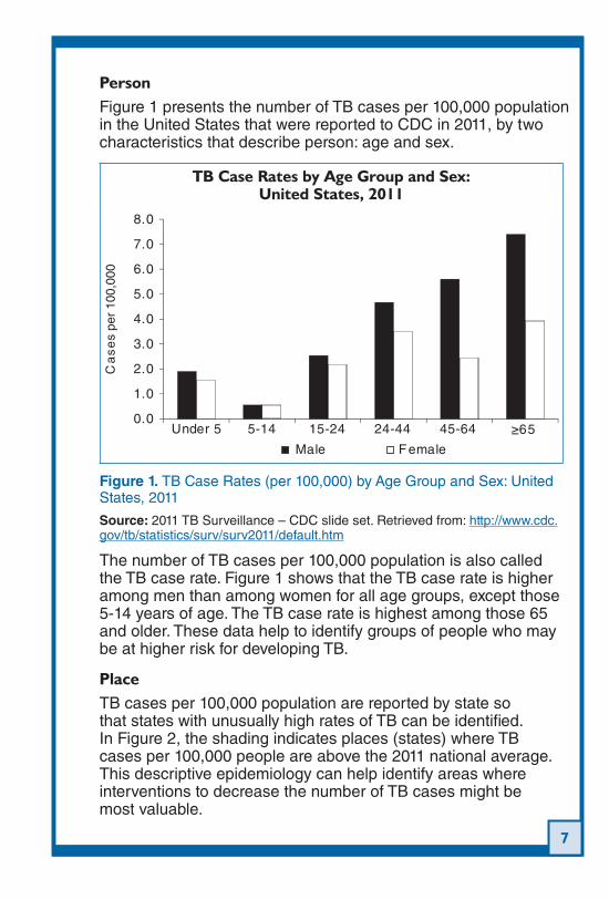
PersonFigure 1 presents the number of TB cases per 100,000 population in the United States that were reported to CDC in 2011, by two characteristics that describe person: age and sex.
TB Case Rates by Age Group and Sex: United States, 2011
Under 5 5-14 15-24 24-44 45-64 ≥65
Male Female
0.0
1.0
2.0
3.0
4.0
5.0
6.0
7.0
8.0
Ca
se
s pe
r 10
0,00
0
Figure 1. TB Case Rates (per 100,000) by Age Group and Sex: United States, 2011
Source: 2011 TB Surveillance – CDC slide set. Retrieved from: http://www.cdc.gov/tb/statistics/surv/surv2011/default.htm
The number of TB cases per 100,000 population is also called the TB case rate. Figure 1 shows that the TB case rate is higher among men than among women for all age groups, except those 5-14 years of age. The TB case rate is highest among those 65 and older. These data help to identify groups of people who may be at higher risk for developing TB.
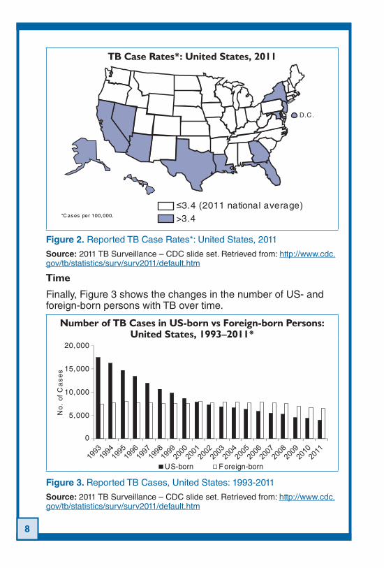
PlaceTB cases per 100,000 population are reported by state so that states with unusually high rates of TB can be identified. In Figure 2, the shading indicates places (states) where TB cases per 100,000 people are above the 2011 national average. This descriptive epidemiology can help identify areas where interventions to decrease the number of TB cases might be most valuable.
8
TB Case Rates*: United States, 2011
*C ases per 100,000.
3.4 (2011 national average)>3.4
D.C .
≥
Figure 2. Reported TB Case Rates*: United States, 2011
Source: 2011 TB Surveillance – CDC slide set. Retrieved from: http://www.cdc.gov/tb/statistics/surv/surv2011/default.htm
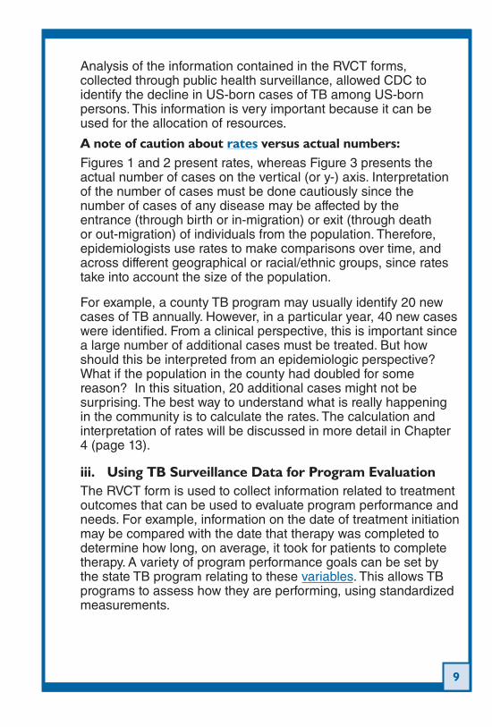
Time
Finally, Figure 3 shows the changes in the number of US- and foreign-born persons with TB over time.
Number of TB Cases in US-born vs Foreign-born Persons: United States, 1993–2011*
No.
of
Ca
se
s
5,000
10,000
15,000
20,000
US-born Foreign-born
0
Figure 3. Reported TB Cases, United States: 1993-2011
Source: 2011 TB Surveillance – CDC slide set. Retrieved from: http://www.cdc.gov/tb/statistics/surv/surv2011/default.htm
9
Analysis of the information contained in the RVCT forms, collected through public health surveillance, allowed CDC to identify the decline in US-born cases of TB among US-born persons. This information is very important because it can be used for the allocation of resources.
A note of caution about rates versus actual numbers:Figures 1 and 2 present rates, whereas Figure 3 presents the actual number of cases on the vertical (or y-) axis. Interpretation of the number of cases must be done cautiously since the number of cases of any disease may be affected by the entrance (through birth or in-migration) or exit (through death or out-migration) of individuals from the population. Therefore, epidemiologists use rates to make comparisons over time, and across different geographical or racial/ethnic groups, since rates take into account the size of the population.
For example, a county TB program may usually identify 20 new cases of TB annually. However, in a particular year, 40 new cases were identified. From a clinical perspective, this is important since a large number of additional cases must be treated. But how should this be interpreted from an epidemiologic perspective? What if the population in the county had doubled for some reason? In this situation, 20 additional cases might not be surprising. The best way to understand what is really happening in the community is to calculate the rates. The calculation and interpretation of rates will be discussed in more detail in Chapter 4 (page 13).
iii. Using TB Surveillance Data for Program EvaluationThe RVCT form is used to collect information related to treatment outcomes that can be used to evaluate program performance and needs. For example, information on the date of treatment initiation may be compared with the date that therapy was completed to determine how long, on average, it took for patients to complete therapy. A variety of program performance goals can be set by the state TB program relating to these variables. This allows TB programs to assess how they are performing, using standardized measurements.
10
In 2006, national priority TB program objectives were established by a team representing TB programs and the Division of Tuberculosis Elimination (DTBE) at CDC. The 15 high-priority TB program objective categories are described in detail in Appendix III (page 107). TB programs that are funded through a cooperative agreement with CDC must report on how well they are achieving these national TB program objectives. Progress toward achieving these program objectives is assessed using the National Tuberculosis Indicators Project (NTIP) monitoring systems. NTIP uses the information that is collected from the RVCT forms and reported to CDC to develop a report that describes TB program progress. These reports can help TB programs evaluate the results of their TB prevention and control activities and prioritize future efforts. A description of NTIP appears in Appendix IV (page 111).
In addition to using surveillance data for program evaluation, TB programs can use clinic records and additional outcome data collected by the programs to evaluate program performance measures. Performance measures can also be evaluated using the cohort review process, which is required of TB programs that are funded through a cooperative agreement with CDC. In a cohort review, the outcomes for each case in a jurisdiction, during a specified time period, are reviewed to identify program successes and areas for improvement. Programs then have an opportunity to implement strategies to improve performance. A description of implementation of the cohort review process is available in the Understanding the TB Cohort Review Process: Instruction Guide (2006). Retrieved from: http://www.cdc.gov/tb/publications/guidestoolkits/cohort/default.htm
The quality of TB surveillance data is dependent on careful data collection, updating, data entry, and transmission. Therefore, the usefulness of the program performance measures that are generated using TB surveillance data is dependent on high-quality surveillance activities. In addition, even for TB programs with high-quality TB surveillance, if they have a small number of TB cases, then one or two cases with a poor outcome can make attaining program performance measures a challenge. Therefore, TB programs with small numbers of cases should be aware of this challenge when interpreting changes in program performance indicators over time.
11
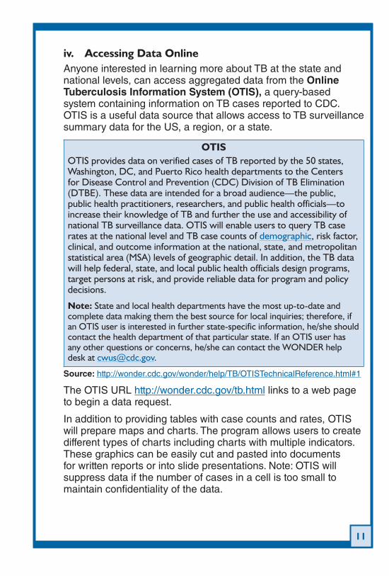
iv. Accessing Data OnlineAnyone interested in learning more about TB at the state and national levels, can access aggregated data from the Online Tuberculosis Information System (OTIS), a query-based system containing information on TB cases reported to CDC. OTIS is a useful data source that allows access to TB surveillance summary data for the US, a region, or a state.
OTISOTIS provides data on verified cases of TB reported by the 50 states, Washington, DC, and Puerto Rico health departments to the Centers for Disease Control and Prevention (CDC) Division of TB Elimination (DTBE). These data are intended for a broad audience—the public, public health practitioners, researchers, and public health officials—to increase their knowledge of TB and further the use and accessibility of national TB surveillance data. OTIS will enable users to query TB case rates at the national level and TB case counts of demographic, risk factor, clinical, and outcome information at the national, state, and metropolitan statistical area (MSA) levels of geographic detail. In addition, the TB data will help federal, state, and local public health officials design programs, target persons at risk, and provide reliable data for program and policy decisions.
Note: State and local health departments have the most up-to-date and complete data making them the best source for local inquiries; therefore, if an OTIS user is interested in further state-specific information, he/she should contact the health department of that particular state. If an OTIS user has any other questions or concerns, he/she can contact the WONDER help desk at [email protected].
Source: http://wonder.cdc.gov/wonder/help/TB/OTISTechnicalReference.html#1
The OTIS URL http://wonder.cdc.gov/tb.html links to a web page to begin a data request.
In addition to providing tables with case counts and rates, OTIS will prepare maps and charts. The program allows users to create different types of charts including charts with multiple indicators. These graphics can be easily cut and pasted into documents for written reports or into slide presentations. Note: OTIS will suppress data if the number of cases in a cell is too small to maintain confidentiality of the data.
12
TB program staff may be interested in learning about the demographic and social characteristics of the population in a state or local area. Information from the US Census and community surveys can be used to describe the population within a particular jurisdiction. These data can be accessed online at the American FactFinder web page http://factfinder2.census.gov/faces/nav/jsf/pages/index.xhtml
CDC has also added TB data to another data query system, called Atlas (see http://www.cdc.gov/nchhstp/atlas/).
B. Analytic EpidemiologyAlthough descriptive epidemiologic data (by person, place, and time) are used to create surveillance summaries or annual reports, analytic epidemiology is used to explain why and how a health problem occurs. One example of an analytic epidemiologic study is when researchers try to identify factors that might predict adherence to treatment.
An excerpt from an article that appeared in the Morbidity and Mortality Weekly Report (MMWR) in 1999 illustrates this point. In this study, the researchers were interested in identifying risk factors for primary multidrug-resistant tuberculosis (P-MDRTB).
“To identify risk factors for P-MDRTB, a case-control study was conducted in February 1999 of never-treated, smear- and culture-positive pulmonary TB patients reported during October 1995-October 1998. A case of P-MDRTB was defined as culture-confirmed MDRTB in a patient; controls were patients with culture-confirmed drug-susceptible TB … compared with controls, case-patients were significantly more likely to have a history of homelessness (23% versus 5%...).”
Source: Primary multidrug-resistant tuberculosis—Ivanovo Oblast, Russia, 1999. Morb Mortal Wkly Rep. 1999;48:661-664.
The researchers found that when comparing P-MDRTB cases (referred to in this study as case-patients) with a comparison group (also called a control group) who had culture-confirmed drug-susceptible TB, “case-patients were significantly more likely to have a history of homelessness.” This is an example of an analytic epidemiologic study because the purpose of the study was to identify risk factors for P-MDRTB. More information on the major types of analytic epidemiology is presented in Chapter 7 of this guide (page 53).
13
Key Concepts in Epidemiology4. As in any other field, epidemiology has its own language or terms that are used to describe events that relate to disease occurrence and outcomes. For example, epidemiology involves the study of morbidity and mortality.
Epidemiology Involves the Study of...
Morbidity:• disease; any departure, subjective or objective, from a state of physiological or psychological health and well-being
Mortality:• death
Source: http://www.cdc.gov/excite/library/glossary.htm
There are various measures that can be used to describe morbidity and mortality.
A. MorbidityMorbidity may be endemic or epidemic. An endemic health condition is one that can be thought of as “usual” or “background” occurrence in a population, whereas epidemic occurrence can be thought of as “unusual” occurrence or occurrence greater than the usual number. When an epidemic occurs in many parts of the world, it is often referred to as a pandemic. If the occurrence of a health condition continues at a very high rate, it may be called hyperendemic. These terms are all relative to the situation in a particular geographic region, so a particular disease rate may be endemic in one country and epidemic in another. Finally, the word outbreak is often used interchangeably with epidemic.
TB is different from many other communicable diseases in that it can take years, sometimes decades, for the disease to develop after infection with Mycobacterium tuberculosis. Thus, a true outbreak of TB generally requires that there be both:
More cases than expected within a geographic area or •population during a particular time period, ANDEvidence of recent transmission of • M. tuberculosis among those cases
The most common way to express morbidity or disease occurrence is by calculating incidence and prevalence measures. Unlike the examination of cases alone, measures of incidence and prevalence allow comparisons across populations and time
14
periods while adjusting for the fact that the number of people in the population may have changed over the same time period.
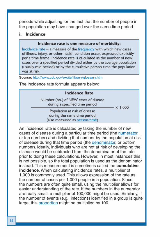
i. Incidence
Incidence rate is one measure of morbidity:Incidence rate – a measure of the frequency with which new cases of illness, injury, or other health condition occur, expressed explicitly per a time frame. Incidence rate is calculated as the number of new cases over a specified period divided either by the average population (usually mid-period) or by the cumulative person-time the population was at risk
Source: http://www.cdc.gov/excite/library/glossary.htm
The incidence rate formula appears below:
Incidence Rate
Number (no.) of NEW cases of disease during a specified time period
× 1,000 Population at risk of disease during the same time period
(also measured as person-time)
An incidence rate is calculated by taking the number of new cases of disease during a particular time period (the numerator, or top number) and dividing that number by the population at risk of disease during that time period (the denominator, or bottom number). Ideally, individuals who are not at risk of developing the disease would be subtracted from the denominator of the rate prior to doing these calculations. However, in most instances this is not possible, so the total population is used as the denominator instead. This measurement is sometimes called the cumulative incidence. When calculating incidence rates, a multiplier of 1,000 is commonly used. This allows expression of the rate as the number of cases per 1,000 people in a population. Since the numbers are often quite small, using the multiplier allows for easier understanding of the rate. If the numbers in the numerator are really small, a multiplier of 100,000 might be used. Similarly, if the number of events (e.g., infections) identified in a group is quite large, this proportion might be multiplied by 100.
15
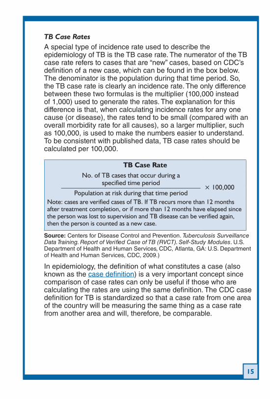
TB Case RatesA special type of incidence rate used to describe the epidemiology of TB is the TB case rate. The numerator of the TB case rate refers to cases that are “new” cases, based on CDC’s definition of a new case, which can be found in the box below. The denominator is the population during that time period. So, the TB case rate is clearly an incidence rate. The only difference between these two formulas is the multiplier (100,000 instead of 1,000) used to generate the rates. The explanation for this difference is that, when calculating incidence rates for any one cause (or disease), the rates tend to be small (compared with an overall morbidity rate for all causes), so a larger multiplier, such as 100,000, is used to make the numbers easier to understand. To be consistent with published data, TB case rates should be calculated per 100,000.
TB Case RateNo. of TB cases that occur during a
specified time period × 100,000
Population at risk during that time periodNote: cases are verified cases of TB. If TB recurs more than 12 months after treatment completion, or if more than 12 months have elapsed since the person was lost to supervision and TB disease can be verified again, then the person is counted as a new case.
Source: Centers for Disease Control and Prevention. Tuberculosis Surveillance Data Training. Report of Verified Case of TB (RVCT). Self-Study Modules. U.S. Department of Health and Human Services, CDC, Atlanta, GA: U.S. Department of Health and Human Services, CDC, 2009.)
In epidemiology, the definition of what constitutes a case (also known as the case definition) is a very important concept since comparison of case rates can only be useful if those who are calculating the rates are using the same definition. The CDC case definition for TB is standardized so that a case rate from one area of the country will be measuring the same thing as a case rate from another area and will, therefore, be comparable.
16
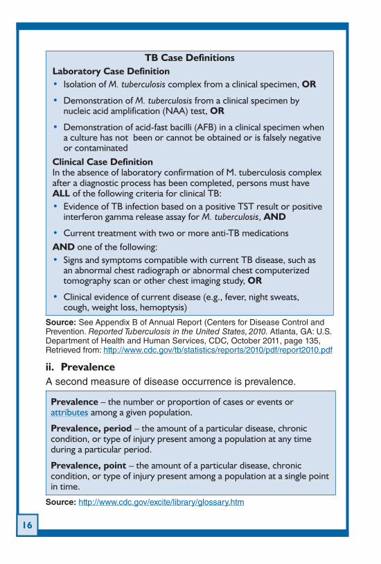
TB Case DefinitionsLaboratory Case Definition
Isolation of • M. tuberculosis complex from a clinical specimen, OR
Demonstration of • M. tuberculosis from a clinical specimen by nucleic acid amplification (NAA) test, OR
Demonstration of acid-fast bacilli (AFB) in a clinical specimen when •a culture has not been or cannot be obtained or is falsely negative or contaminated
Clinical Case Definition In the absence of laboratory confirmation of M. tuberculosis complex after a diagnostic process has been completed, persons must have ALL of the following criteria for clinical TB:
Evidence of TB infection based on a positive TST result or positive •interferon gamma release assay for M. tuberculosis, AND
Current treatment with two or more anti-TB medications•AND one of the following:
Signs and symptoms compatible with current TB disease, such as •an abnormal chest radiograph or abnormal chest computerized tomography scan or other chest imag ing study, OR
Clinical evidence of current disease (e.g., fever, night sweats, •cough, weight loss, hemoptysis)
Source: See Appendix B of Annual Report (Centers for Disease Control and Prevention. Reported Tuberculosis in the United States, 2010. Atlanta, GA: U.S. Department of Health and Human Services, CDC, October 2011, page 135, Retrieved from: http://www.cdc.gov/tb/statistics/reports/2010/pdf/report2010.pdf
ii. PrevalenceA second measure of disease occurrence is prevalence.
Prevalence – the number or proportion of cases or events or attributes among a given population.
Prevalence, period – the amount of a particular disease, chronic condition, or type of injury present among a population at any time during a particular period.
Prevalence, point – the amount of a particular disease, chronic condition, or type of injury present among a population at a single point in time.
Source: http://www.cdc.gov/excite/library/glossary.htm
17
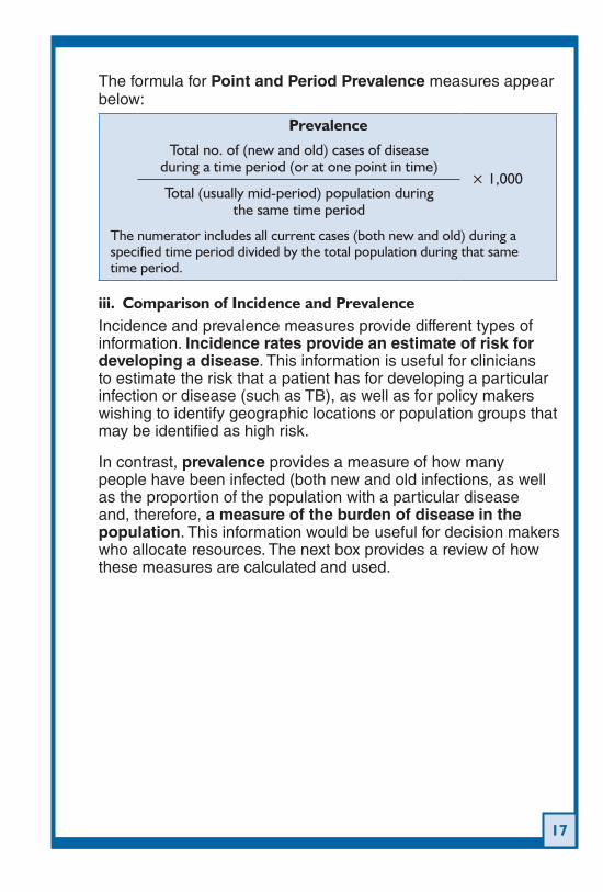
The formula for Point and Period Prevalence measures appear below:
Prevalence
Total no. of (new and old) cases of disease during a time period (or at one point in time)
× 1,000Total (usually mid-period) population during
the same time period
The numerator includes all current cases (both new and old) during a specified time period divided by the total population during that same time period.
iii. Comparison of Incidence and PrevalenceIncidence and prevalence measures provide different types of information. Incidence rates provide an estimate of risk for developing a disease. This information is useful for clinicians to estimate the risk that a patient has for developing a particular infection or disease (such as TB), as well as for policy makers wishing to identify geographic locations or population groups that may be identified as high risk.
In contrast, prevalence provides a measure of how many people have been infected (both new and old infections, as well as the proportion of the population with a particular disease and, therefore, a measure of the burden of disease in the population. This information would be useful for decision makers who allocate resources. The next box provides a review of how these measures are calculated and used.
18
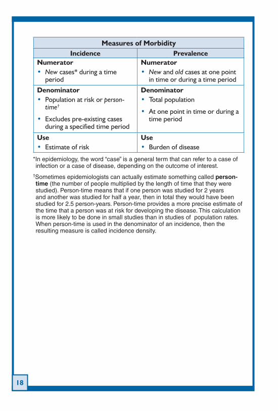
Measures of MorbidityIncidence Prevalence
NumeratorNew• cases* during a time period
NumeratorNew• and old cases at one point in time or during a time period
DenominatorPopulation at risk or • person-time†
Excludes pre-existing cases •during a specified time period
DenominatorTotal population•
At one point in time or during a •time period
UseEstimate of risk•
UseBurden of disease•
*In epidemiology, the word “case” is a general term that can refer to a case of infection or a case of disease, depending on the outcome of interest.
†Sometimes epidemiologists can actually estimate something called person-time (the number of people multiplied by the length of time that they were studied). Person-time means that if one person was studied for 2 years and another was studied for half a year, then in total they would have been studied for 2.5 person-years. Person-time provides a more precise estimate of the time that a person was at risk for developing the disease. This calculation is more likely to be done in small studies than in studies of population rates. When person-time is used in the denominator of an incidence, then the resulting measure is called incidence density.
19
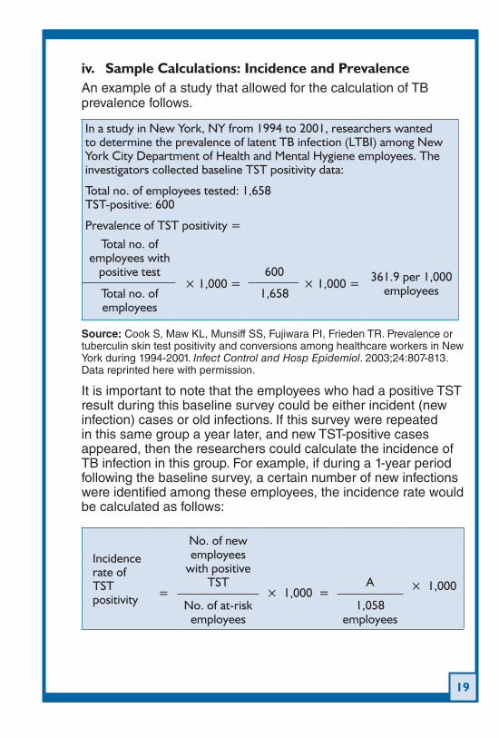
iv. Sample Calculations: Incidence and PrevalenceAn example of a study that allowed for the calculation of TB prevalence follows.
In a study in New York, NY from 1994 to 2001, researchers wanted to determine the prevalence of latent TB infection (LTBI) among New York City Department of Health and Mental Hygiene employees. The investigators collected baseline TST positivity data:
Total no. of employees tested: 1,658TST-positive: 600
Prevalence of TST positivity =Total no. of
employees with positive test
× 1,000 =
600 × 1,000 =
361.9 per 1,000
employeesTotal no. of employees
1,658
Source: Cook S, Maw KL, Munsiff SS, Fujiwara PI, Frieden TR. Prevalence or tuberculin skin test positivity and conversions among healthcare workers in New York during 1994-2001. Infect Control and Hosp Epidemiol. 2003;24:807-813. Data reprinted here with permission.
It is important to note that the employees who had a positive TST result during this baseline survey could be either incident (new infection) cases or old infections. If this survey were repeated in this same group a year later, and new TST-positive cases appeared, then the researchers could calculate the incidence of TB infection in this group. For example, if during a 1-year period following the baseline survey, a certain number of new infections were identified among these employees, the incidence rate would be calculated as follows:
Incidence rate of TST positivity
=
No. of new employees
with positive TST
× 1,000 =
A
× 1,000
No. of at-risk employees
1,058 employees
20
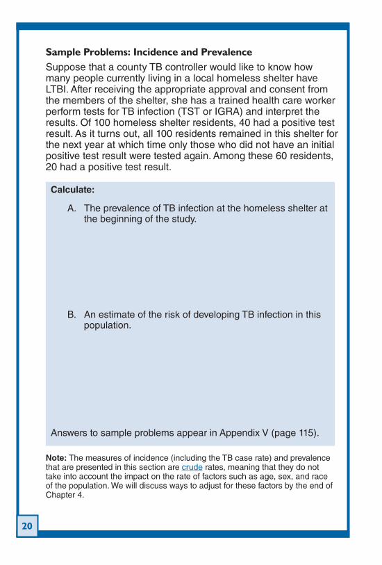
Sample Problems: Incidence and PrevalenceSuppose that a county TB controller would like to know how many people currently living in a local homeless shelter have LTBI. After receiving the appropriate approval and consent from the members of the shelter, she has a trained health care worker perform tests for TB infection (TST or IGRA) and interpret the results. Of 100 homeless shelter residents, 40 had a positive test result. As it turns out, all 100 residents remained in this shelter for the next year at which time only those who did not have an initial positive test result were tested again. Among these 60 residents, 20 had a positive test result.
Calculate:
The prevalence of TB infection at the homeless shelter at A. the beginning of the study.
An estimate of the risk of developing TB infection in this B. population.
Answers to sample problems appear in Appendix V (page 115).
Note: The measures of incidence (including the TB case rate) and prevalence that are presented in this section are crude rates, meaning that they do not take into account the impact on the rate of factors such as age, sex, and race of the population. We will discuss ways to adjust for these factors by the end of Chapter 4.
21
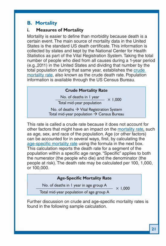
B. Mortalityi. Measures of MortalityMortality is easier to define than morbidity because death is a certain event. The main source of mortality data in the United States is the standard US death certificate. This information is collected by states and kept by the National Center for Health Statistics as part of the Vital Registration System. Taking the total number of people who died from all causes during a 1-year period (e.g.,2011) in the United States and dividing that number by the total population during that same year, establishes the crude mortality rate, also known as the crude death rate. Population information is available through the US Census Bureau.
Crude Mortality RateNo. of deaths in 1 year
× 1,000Total mid-year population
No. of deaths Vital Registration SystemTotal mid-year population Census Bureau
This rate is called a crude rate because it does not account for other factors that might have an impact on the mortality rate, such as age, sex, and race of the population. Age (or other factors) can be accounted for in several ways, first, by calculating the age-specific mortality rate using the formula in the next box. This calculation reports the death rate for a segment of the population within a specific age range. “Specific” applies to both the numerator (the people who die) and the denominator (the people at risk). The death rate may be calculated per 100, 1,000, or 100,000.
Age-Specific Mortality Rate
No. of deaths in 1 year in age group A× 1,000
Total mid-year population of age group A
Further discussion on crude and age-specific mortality rates is found in the following sample calculation.
22
ii. Sample Calculations of Crude and Age-Specific Mortality Rates
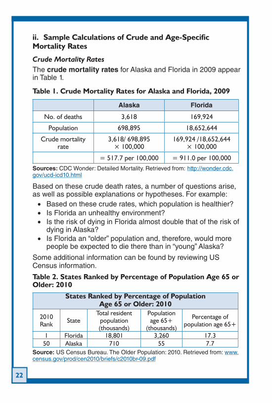
Crude Mortality RatesThe crude mortality rates for Alaska and Florida in 2009 appear in Table 1.
Table 1. Crude Mortality Rates for Alaska and Florida, 2009
Alaska Florida
No. of deaths 3,618 169,924
Population 698,895 18,652,644
Crude mortality rate
3,618/ 698,895 × 100,000
169,924 /18,652,644 × 100,000
= 517.7 per 100,000 = 911.0 per 100,000Sources: CDC Wonder: Detailed Mortality. Retrieved from: http://wonder.cdc.gov/ucd-icd10.html
Based on these crude death rates, a number of questions arise, as well as possible explanations or hypotheses. For example:
Based on these crude rates, which population is healthier?•Is Florida an unhealthy environment?•Is the risk of dying in Florida almost double that of the risk of •dying in Alaska?Is Florida an “older” population and, therefore, would more •people be expected to die there than in “young” Alaska?
Some additional information can be found by reviewing US Census information.
Table 2. States Ranked by Percentage of Population Age 65 or Older: 2010
States Ranked by Percentage of Population Age 65 or Older: 2010
2010 Rank State
Total resident population (thousands)
Population age 65+
(thousands)
Percentage of population age 65+
1 Florida 18,801 3,260 17.350 Alaska 710 55 7.7
Source: US Census Bureau. The Older Population: 2010. Retrieved from: www.census.gov/prod/cen2010/briefs/c2010br-09.pdf
23
The US Census Bureau information reveals that Florida has the highest percentage of people 65 years of age or older, and Alaska has the lowest, suggesting that some of the difference in mortality could be explained by the different age distributions of these populations. One way to adjust or control for the difference in age distribution and to answer some of the previous questions is to calculate age-specific mortality rates.
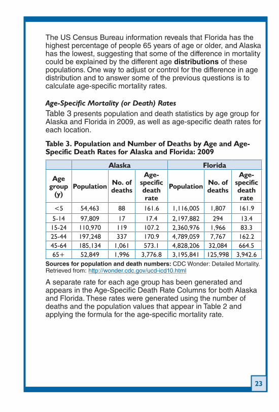
Age-Specific Mortality (or Death) RatesTable 3 presents population and death statistics by age group for Alaska and Florida in 2009, as well as age-specific death rates for each location.
Table 3. Population and Number of Deaths by Age and Age-Specific Death Rates for Alaska and Florida: 2009
Alaska Florida
Age group
(y)Population No. of
deaths
Age-specific death rate
Population No. of deaths
Age-specific death rate
<5 54,463 88 161.6 1,116,005 1,807 161.9
5-14 97,809 17 17.4 2,197,882 294 13.415-24 110,970 119 107.2 2,360,976 1,966 83.325-44 197,248 337 170.9 4,789,059 7,767 162.245-64 185,134 1,061 573.1 4,828,206 32,084 664.565+ 52,849 1,996 3,776.8 3,195,841 125,998 3,942.6
Sources for population and death numbers: CDC Wonder: Detailed Mortality. Retrieved from: http://wonder.cdc.gov/ucd-icd10.html
A separate rate for each age group has been generated and appears in the Age-Specific Death Rate Columns for both Alaska and Florida. These rates were generated using the number of deaths and the population values that appear in Table 2 and applying the formula for the age-specific mortality rate.
24
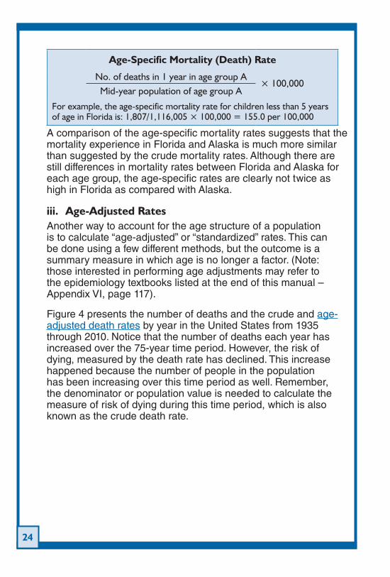
Age-Specific Mortality (Death) Rate
No. of deaths in 1 year in age group A× 100,000
Mid-year population of age group A
For example, the age-specific mortality rate for children less than 5 years of age in Florida is: 1,807/1,116,005 × 100,000 = 155.0 per 100,000
A comparison of the age-specific mortality rates suggests that the mortality experience in Florida and Alaska is much more similar than suggested by the crude mortality rates. Although there are still differences in mortality rates between Florida and Alaska for each age group, the age-specific rates are clearly not twice as high in Florida as compared with Alaska.
iii. Age-Adjusted RatesAnother way to account for the age structure of a population is to calculate “age-adjusted” or “standardized” rates. This can be done using a few different methods, but the outcome is a summary measure in which age is no longer a factor. (Note: those interested in performing age adjustments may refer to the epidemiology textbooks listed at the end of this manual – Appendix VI, page 117).
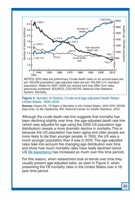
Figure 4 presents the number of deaths and the crude and age-adjusted death rates by year in the United States from 1935 through 2010. Notice that the number of deaths each year has increased over the 75-year time period. However, the risk of dying, measured by the death rate has declined. This increase happened because the number of people in the population has been increasing over this time period as well. Remember, the denominator or population value is needed to calculate the measure of risk of dying during this time period, which is also known as the crude death rate.
25
Nu
mb
er
of
de
ath
s (m
illio
ns)
0
1.0
1.2
1.4
1.6
1.8
2.0
2.2
2.4
201020001990198019701960195019401935
0
De
ath
s pe
r 10
0,0
00
po
pu
latio
n800
1000
1200
1400
1600
1800
2000
Age-adjusteddeath rate
Number ofdeaths
1,860.1
1,094.5
1,392,752
1,314.8
919.0
967.9
1,304.5
798.7
2,465,936
746.2
Crude deathrate
NOTES: 2010 data are preliminary. Crude death rates on an annual basis are per 100,000 population; age-adjusted rates are per 100,000 U.S. standard population. Rates for 2001–2009 are revised and may differ from rates previously published. SOURCE: CDC/NCHS, National Vital Statistics System, Mortality.
Figure 4. Number of Deaths, Crude and Age-adjusted Death Rates: United States, 1935–2010Source: Hoyert DL. 75 Years of Mortality in the United States 1935-2010. NCHS data brief, no 88. Hyattsville, MD: National Center for Health Statistics, 2012.
Although the crude death rate line suggests that mortality has been declining slightly over time, the age-adjusted death rate line (which was adjusted for age using the 2000 US population age distribution) reveals a more dramatic decline in mortality. This is because the US population has been aging and older people are more likely to die than younger people; in 1935, the US was a much younger population than it was in 2010. The age-adjusted rates take into account the changing age distribution over time and show how much mortality rates have really declined (since US life expectancy has increased so much over this time period).
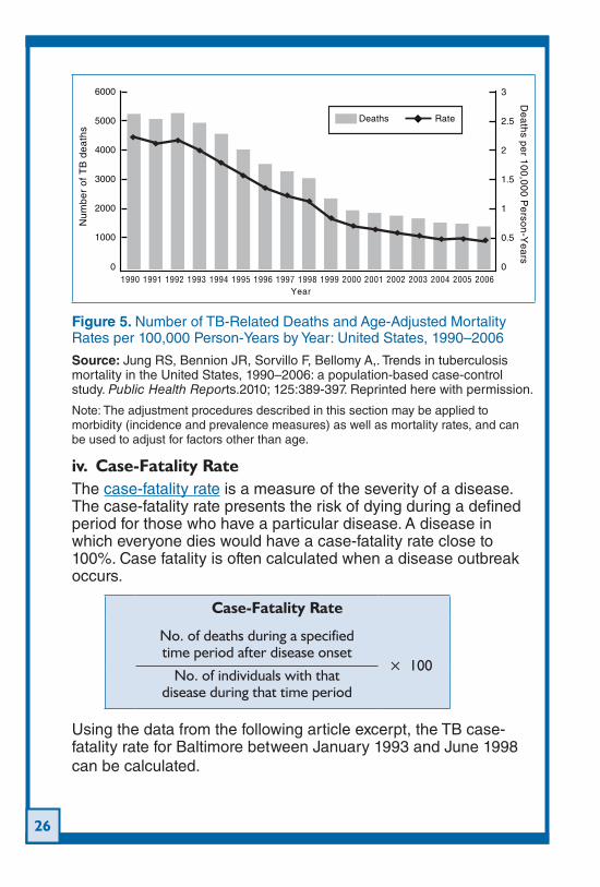
For this reason, when researchers look at trends over time they usually present age-adjusted rates, as seen in Figure 5, when presenting the TB mortality rates in the United States over a 16-year time period.
26
Nu
mb
er
of
TB
de
ath
s
0
1000
2000
3000
4000
5000
6000
20062005200420021993199219911990
De
ath
s pe
r 10
0,0
00
Pe
rson
-Ye
ars
0
0.5
1
1.5
2
2.5
3
Deaths Rate
1997199619951994 2001200019991998 2003Year
Figure 5. Number of TB-Related Deaths and Age-Adjusted Mortality Rates per 100,000 Person-Years by Year: United States, 1990–2006
Source: Jung RS, Bennion JR, Sorvillo F, Bellomy A,. Trends in tuberculosis mortality in the United States, 1990–2006: a population-based case-control study. Public Health Reports.2010; 125:389-397. Reprinted here with permission.
Note: The adjustment procedures described in this section may be applied to morbidity (incidence and prevalence measures) as well as mortality rates, and can be used to adjust for factors other than age.
iv. Case-Fatality RateThe case-fatality rate is a measure of the severity of a disease. The case-fatality rate presents the risk of dying during a defined period for those who have a particular disease. A disease in which everyone dies would have a case-fatality rate close to 100%. Case fatality is often calculated when a disease outbreak occurs.
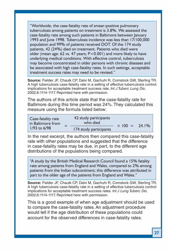
Case-Fatality Rate
No. of deaths during a specified time period after disease onset
× 100No. of individuals with that
disease during that time period
Using the data from the following article excerpt, the TB case-fatality rate for Baltimore between January 1993 and June 1998 can be calculated.
27
“Worldwide, the case-fatality rate of smear-positive pulmonary tuberculosis among patients on treatment is 3.8%. We assessed the case-fatality rate among such patients in Baltimore between January 1993 and June 1998. Tuberculosis incidence was less than 17/100,000 population and 99% of patients received DOT. Of the 174 study patients, 42 (24%) died on treatment. Patients who died were older (mean age: 62 vs. 47 years; P<0.001) and more likely to have underlying medical conditions. With effective control, tuberculosis may become concentrated in older persons with chronic diseases and be associated with high case-fatality rates. In such settings, acceptable treatment success rates may need to be revised.”
Source: Fielder JF, Chaulk CP, Dalvi M, Gachuhi R, Comstock GW, Sterling TR. A high tuberculosis case-fatality rate in a setting of effective tuberculosis control: implications for acceptable treatment success rate. Int J Tuberc Lung Dis. 2002;6:1114-1117. Reprinted here with permission.
The authors of this article state that the case-fatality rate for Baltimore during this time period was 24%. They calculated this measure using the formula listed below:
Case-fatality rate in Baltimore from 1/93 to 6/98
=
42 study participants who died
× 100 =
24.1% 174 study participants
In the next excerpt, the authors then compared this case-fatality rate with other populations and suggested that the difference in case-fatality rates may be due, in part, to the different age distributions of the populations being compared.
“A study by the British Medical Research Council found a 15% fatality rate among patients from England and Wales, compared to 2% among patients from the Indian subcontinent; this difference was attributed in part to the older age of the patients from England and Wales.”
Source: Fielder JF, Chaulk CP, Dalvi M, Gachuhi R, Comstock GW, Sterling TR. A high tuberculosis case-fatality rate in a setting of effective tuberculosis control: implications for acceptable treatment success rates. Int J Lung Tuberc Dis. 2002;6:1114-1117. Reprinted here with permission.
This is a good example of when age adjustment should be used to compare the case-fatality rates. An adjustment procedure would tell if the age distribution of these populations could account for the observed differences in case-fatality rates.
28
Sample Problems: Case-Fatality RateIn the previous article, the authors stated that “A study by the British Medical Research Council found a 15% fatality rate among patients from England and Wales, compared to 2% among patients from the Indian subcontinent; this difference was attributed in part to the older age of the patients from England and Wales.”
A. With a 15% case-fatality rate, if 100 people had TB, how many would die during the study period?
B. Why did the authors attribute the difference in case-fatality rate in England and Wales compared with the rate from the Indian subcontinent in part to the age distribution of these patients?
Answers to these questions can be found in Appendix V (page 115).
29
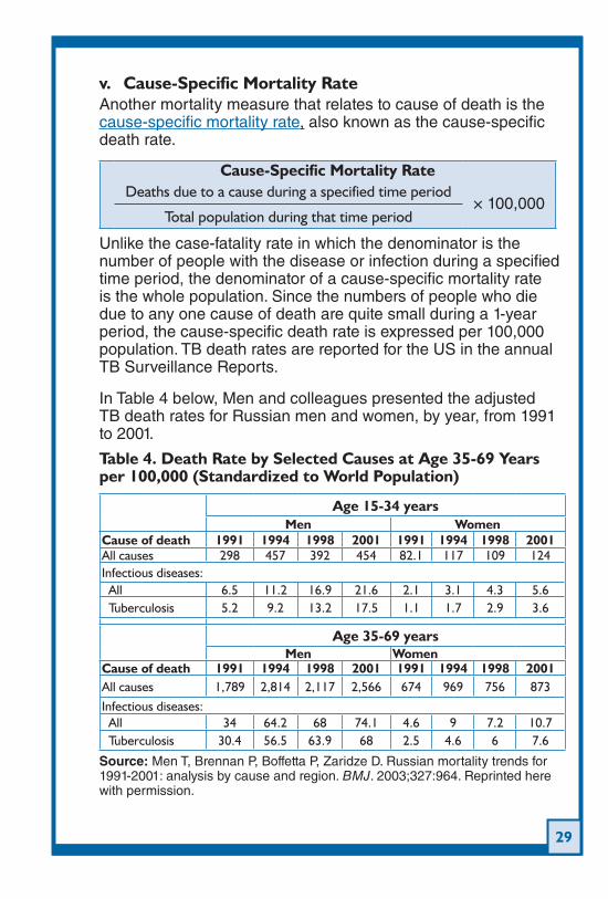
v. Cause-Specific Mortality RateAnother mortality measure that relates to cause of death is the cause-specific mortality rate, also known as the cause-specific death rate.
Cause-Specific Mortality RateDeaths due to a cause during a specified time period
× 100,000Total population during that time period
Unlike the case-fatality rate in which the denominator is the number of people with the disease or infection during a specified time period, the denominator of a cause-specific mortality rate is the whole population. Since the numbers of people who die due to any one cause of death are quite small during a 1-year period, the cause-specific death rate is expressed per 100,000 population. TB death rates are reported for the US in the annual TB Surveillance Reports.
In Table 4 below, Men and colleagues presented the adjusted TB death rates for Russian men and women, by year, from 1991 to 2001.
Table 4. Death Rate by Selected Causes at Age 35-69 Years per 100,000 (Standardized to World Population)
Age 15-34 yearsMen Women
Cause of death 1991 1994 1998 2001 1991 1994 1998 2001All causes 298 457 392 454 82.1 117 109 124Infectious diseases: All 6.5 11.2 16.9 21.6 2.1 3.1 4.3 5.6 Tuberculosis 5.2 9.2 13.2 17.5 1.1 1.7 2.9 3.6
Age 35-69 yearsMen Women
Cause of death 1991 1994 1998 2001 1991 1994 1998 2001All causes 1,789 2,814 2,117 2,566 674 969 756 873Infectious diseases: All 34 64.2 68 74.1 4.6 9 7.2 10.7 Tuberculosis 30.4 56.5 63.9 68 2.5 4.6 6 7.6
Source: Men T, Brennan P, Boffetta P, Zaridze D. Russian mortality trends for 1991-2001: analysis by cause and region. BMJ. 2003;327:964. Reprinted here with permission.
30
The table shows that during this time period: 1) the cause-specific death rates for TB were higher in men than in women; 2) the cause-specific death rates for TB were increasing for both men and women and for both age groups; and 3) the death rates for men 35-69 years of age were much higher than for the younger aged men (15-34 years).
Sample Problem: Cause-Specific Mortality Rate
A. What type of TB rates is presented in Table 4?
Answer to this question can be found in Appendix V (page 115).
Something to think about…
The completeness of the morbidity data that are used to calculate incidence and prevalence measures is dependent on a number of factors including the willingness or ability of the individual to seek health care; the severity of the illness; the type of public health surveillance required by law; the decision of the health care provider to report the illness; and the quality of the tests used to identify the disease or infection. Chapter 6 of the manual (page 46) will demonstrate how to measure the value of a diagnostic test.
When compared with morbidity data, mortality data are usually of much higher quality due to the certainty of the event and the fact that in the United States almost all deaths are reported to the appropriate authorities. However, many studies have shown that information on death certificates is not always accurate. For example, information on the age, marital status, and usual occupation of the person who has died is collected when the funeral director asks the person in charge of funeral
31
arrangements to provide it. If that individual does not know the correct answers to these questions, the information may not be accurately reported. The information on the cause of death on a death certificate may also be subject to errors, either because the person reporting this information incorrectly identifies the cause of death or if it is coded incorrectly on the form. Cause of death information is more accurate when an autopsy is done to identify the cause and when medical records are available to those who are completing the cause of death section of the death certificate. References that relate to the accuracy of death certificate data for those with TB appear in the suggested reading list in Appendix VI (page 117).
These factors are all important considerations whenever examining morbidity and mortality data.
Note: Since the purpose of this manual is to illustrate how epidemiologic measures can be used in US TB programs, the examples presented are almost exclusively using US data. However, the World Health Organization is an excellent source of international TB morbidity and mortality data; see http://www.who.int/tb/publications/global_report/en/index.html for the WHO report entitled Global Tuberculosis Control 2012.
32
Presenting TB Program Data5. A. Measurement ScalesIn traditional epidemiologic studies, data are collected on study subjects using three basic measurement scales: nominal, ordinal, and numerical. A nominal scale is used to record categorical data. Race, sex, and place of residence are examples of nominal data. An ordinal scale is used to collect information, which has some order, but the distance between each point on the scale is not necessarily the same. For example, patients are often described as having Stage I, II, III, or IV cancer. Stage IV is a more advanced stage of the disease than Stage II, but Stage IV is not necessarily twice as severe as Stage II. Finally, data are often collected on a numerical scale. Numerical data include discrete variables such as the number of prior pregnancies or continuous variables such as blood pressure or body weight.
In addition to data collected on nominal, ordinal, or numerical scales, respondents may be asked to describe their feelings about a particular treatment or about their health using open-ended questions These open-ended questions allow the researchers to collect qualitative information through an analysis of the language the respondents use rather than having the respondent choose from supplied answers as in multiple choice questions. An example an open-ended question is: “Please describe anything that you believe made it difficult for you to complete your treatment for latent tuberculosis infection.” Once these responses are transcribed, they can be analyzed using a qualitative data analysis software package or coded by themes and analyzed as nominal data. Combining quantitative and qualitative techniques can provide a rich source of information and can be used to validate responses.
B. Summarizing the DataTB program data can be summarized and presented in a number of ways. When summarizing data measures that describe the central location or middle of the data are often presented as well as how much variation or spread there is in a particular data set. The types of summary measures and graphs that are appropriate for presenting data will depend, in part, on the type of scale
33
(nominal, ordinal, or numerical) that was used to collect these data. Some common measures and data displays are described in this section.
Definitions of Summary Measures
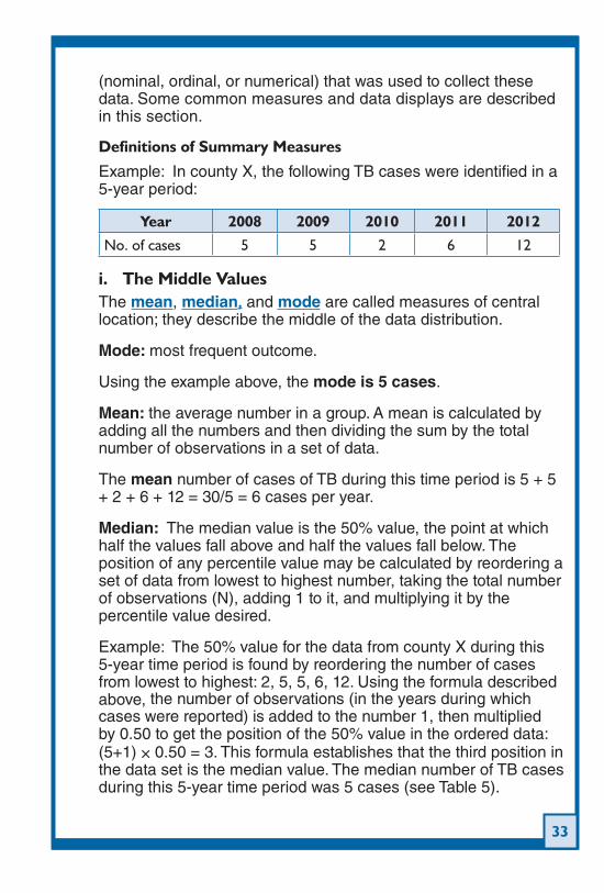
Example: In county X, the following TB cases were identified in a 5-year period:
Year 2008 2009 2010 2011 2012
No. of cases 5 5 2 6 12
i. The Middle ValuesThe mean, median, and mode are called measures of central location; they describe the middle of the data distribution.
Mode: most frequent outcome.
Using the example above, the mode is 5 cases.
Mean: the average number in a group. A mean is calculated by adding all the numbers and then dividing the sum by the total number of observations in a set of data.
The mean number of cases of TB during this time period is 5 + 5 + 2 + 6 + 12 = 30/5 = 6 cases per year.
Median: The median value is the 50% value, the point at which half the values fall above and half the values fall below. The position of any percentile value may be calculated by reordering a set of data from lowest to highest number, taking the total number of observations (N), adding 1 to it, and multiplying it by the percentile value desired.
Example: The 50% value for the data from county X during this 5-year time period is found by reordering the number of cases from lowest to highest: 2, 5, 5, 6, 12. Using the formula described above, the number of observations (in the years during which cases were reported) is added to the number 1, then multiplied by 0.50 to get the position of the 50% value in the ordered data: (5+1) × 0.50 = 3. This formula establishes that the third position in the data set is the median value. The median number of TB cases during this 5-year time period was 5 cases (see Table 5).
34
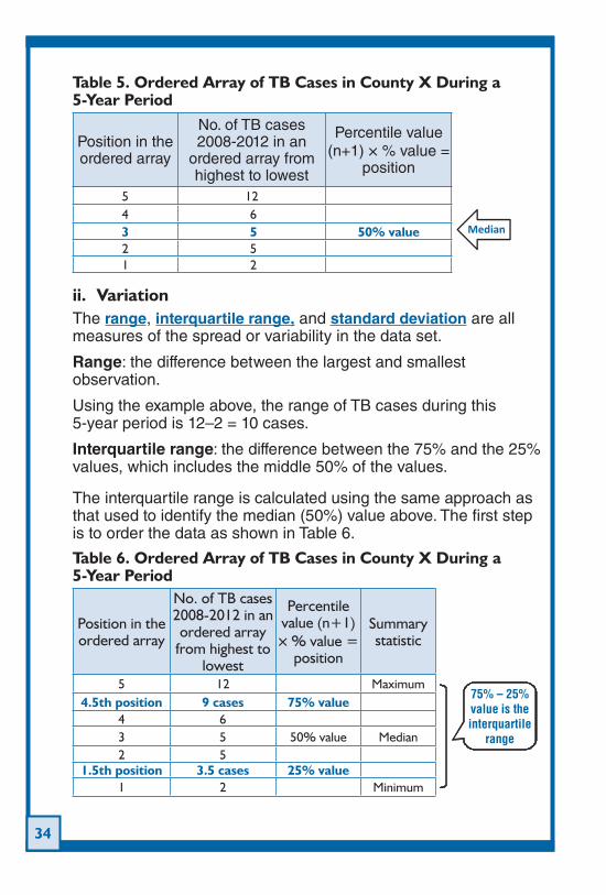
Table 5. Ordered Array of TB Cases in County X During a 5-Year Period
Position in the ordered array
No. of TB cases 2008-2012 in an
ordered array from highest to lowest
Percentile value (n+1) × % value =
position
5 12
Median
4 63 5 50% value2 51 2
ii. VariationThe range, interquartile range, and standard deviation are all measures of the spread or variability in the data set.
Range: the difference between the largest and smallest observation.
Using the example above, the range of TB cases during this 5-year period is 12–2 = 10 cases.
Interquartile range: the difference between the 75% and the 25% values, which includes the middle 50% of the values.
The interquartile range is calculated using the same approach as that used to identify the median (50%) value above. The first step is to order the data as shown in Table 6.
Table 6. Ordered Array of TB Cases in County X During a 5-Year Period
Position in the ordered array
No. of TB cases 2008-2012 in an ordered array
from highest to lowest
Percentile value (n+1) × % value =
position
Summary statistic
5 12 Maximum75% – 25% value is the interquartile
range
4.5th position 9 cases 75% value4 63 5 50% value Median2 5
1.5th position 3.5 cases 25% value1 2 Minimum
35
Using the formula described above—(n+1) × the percentile value—the number 1 is added to the number of observations (in the years in which cases were reported), then multiplied by 0.75 to get the position of the 75% value in the ordered data: (5+1) × 0.75 = 4.5th position in the ordered list.
Then using the same process, the 25% value is determined: (5+1) × 0.25 = 1.5th position in the ordered list. The 4.5th position has a value half way between the 4th (6 TB cases) and 5th (12 TB cases) values (i.e., 9 TB cases). The 1.5th position has a value half way between the 1st (2 TB cases) and the 2nd (5 TB cases), so it is 3.5 TB cases. The values that appear in blue in Table 6 above are called interpolated values.
The interquartile range could then be calculated as 9 TB cases: 3.5 TB cases = 5.5 TB cases. This is a measure of how much variation there is in the number of TB cases reported during this 5-year period.
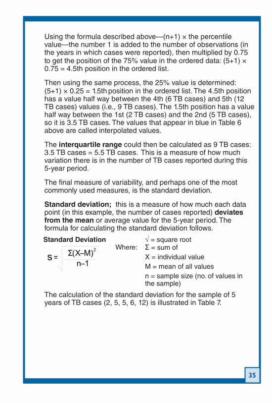
The final measure of variability, and perhaps one of the most commonly used measures, is the standard deviation.
Standard deviation; this is a measure of how much each data point (in this example, the number of cases reported) deviates from the mean or average value for the 5-year period. The formula for calculating the standard deviation follows.
Standard Deviation √ = square root
n 1–s = Σ(X M)– 2 Where: Σ = sum of
X = individual valueM = mean of all valuesn = sample size (no. of values in the sample)
The calculation of the standard deviation for the sample of 5 years of TB cases (2, 5, 5, 6, 12) is illustrated in Table 7.
36
Table 7. Example of Standard Deviation Calculation
A B C D E F GIndividual
value Mean X-mean (X-mean)2 (X-mean)2 n–1
Square root
Standard deviation
2 6 –4 165 6 –1 15 6 –1 16 6 0 0
12 6 6 36Σ or sum Σ54 54/4 = √13.5 3.67
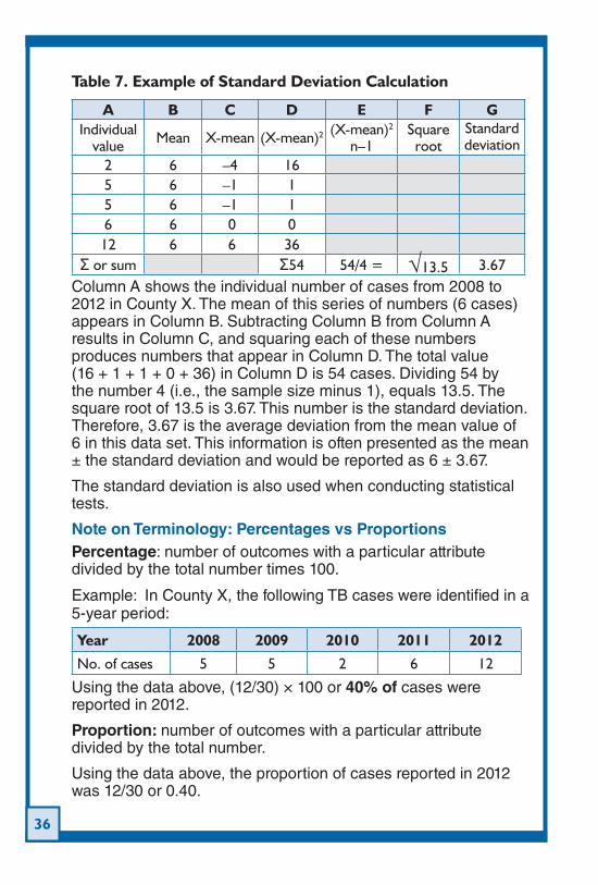
Column A shows the individual number of cases from 2008 to 2012 in County X. The mean of this series of numbers (6 cases) appears in Column B. Subtracting Column B from Column A results in Column C, and squaring each of these numbers produces numbers that appear in Column D. The total value (16 + 1 + 1 + 0 + 36) in Column D is 54 cases. Dividing 54 by the number 4 (i.e., the sample size minus 1), equals 13.5. The square root of 13.5 is 3.67. This number is the standard deviation. Therefore, 3.67 is the average deviation from the mean value of 6 in this data set. This information is often presented as the mean ± the standard deviation and would be reported as 6 ± 3.67.
The standard deviation is also used when conducting statistical tests.
Note on Terminology: Percentages vs ProportionsPercentage: number of outcomes with a particular attribute divided by the total number times 100.
Example: In County X, the following TB cases were identified in a 5-year period:
Year 2008 2009 2010 2011 2012
No. of cases 5 5 2 6 12
Using the data above, (12/30) × 100 or 40% of cases were reported in 2012.
Proportion: number of outcomes with a particular attribute divided by the total number.
Using the data above, the proportion of cases reported in 2012 was 12/30 or 0.40.
37
iii. Which Measures to Use?For data measured on a nominal scale, the mode and percentile values are the most common summary measures.
For data measured on an ordinal scale, the most common summary measures of the center of the distribution are the median and mode, and the most common measures of variability are the interquartile range and range.
When deciding how to present data that is measured on a numeric scale, it must be determined if the distribution of the data are normally distributed or skewed. Normally distributed data are unimodal (one hump) and symmetric (a line can be put through the middle and each side is a mirror image of the other). This type of curve is often referred to as a normal or bell-shaped curve. When looking at these curves, try to imagine a number line underneath each of them, with the lower numbers on the far left and the higher numbers on the far right. These numbers might represent the number of TB cases over some time period or even TB case rates.
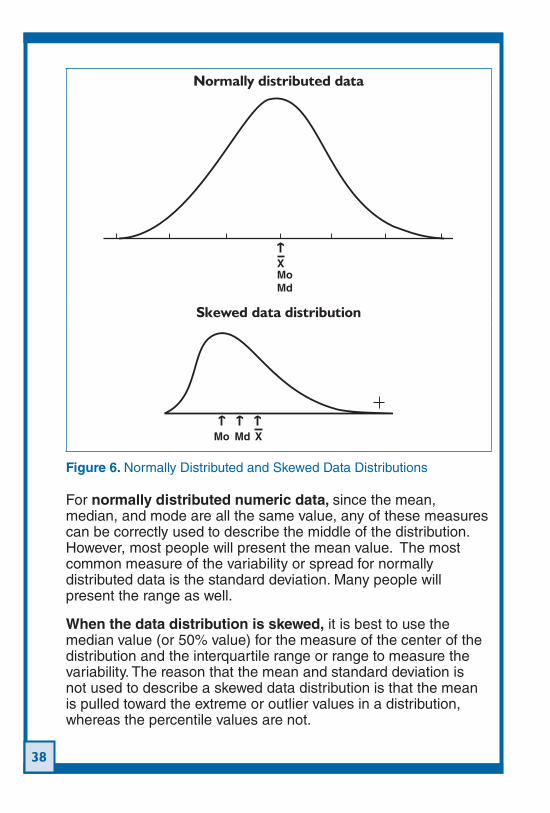
For perfectly normally distributed data, the mean, median, and mode for a particular set of data are all the same value. For non-normally distributed (skewed) data, the mean (represented as an X with a line over it called X bar) is pulled toward the extreme value in the skewed distribution. Extreme values are unusually high or low values in a data set and are also known as outliers. Figure 6 provides examples of normal and skewed data distributions. The bottom of each distribution shows how the mode (Mo), median (Md), and mean (X bar) are affected by the distribution of the data. The extreme value in the skewed distribution is indicated by the plus sign (+) on the far right. This skewed distribution is described as right or positively skewed or skewed toward high numbers. If the unusual or outlier observation had been very low and the tail of the distribution (the thinner part under the curve) had been on the left side of the distribution, then it would be called left or negatively skewed or skewed toward lower numbers.
38
Normally distributed data
XMoMd
Skewed data distribution
XMo Md
Figure 6. Normally Distributed and Skewed Data Distributions
For normally distributed numeric data, since the mean, median, and mode are all the same value, any of these measures can be correctly used to describe the middle of the distribution. However, most people will present the mean value. The most common measure of the variability or spread for normally distributed data is the standard deviation. Many people will present the range as well.
When the data distribution is skewed, it is best to use the median value (or 50% value) for the measure of the center of the distribution and the interquartile range or range to measure the variability. The reason that the mean and standard deviation is not used to describe a skewed data distribution is that the mean is pulled toward the extreme or outlier values in a distribution, whereas the percentile values are not.
39
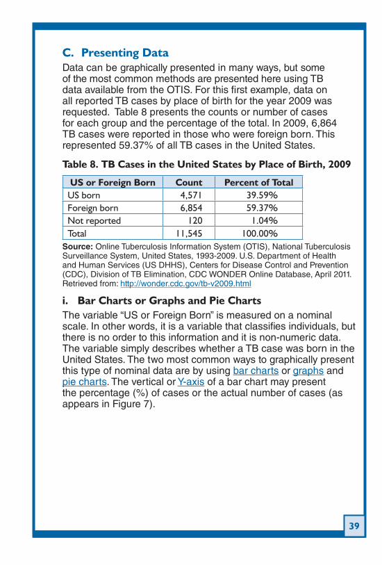
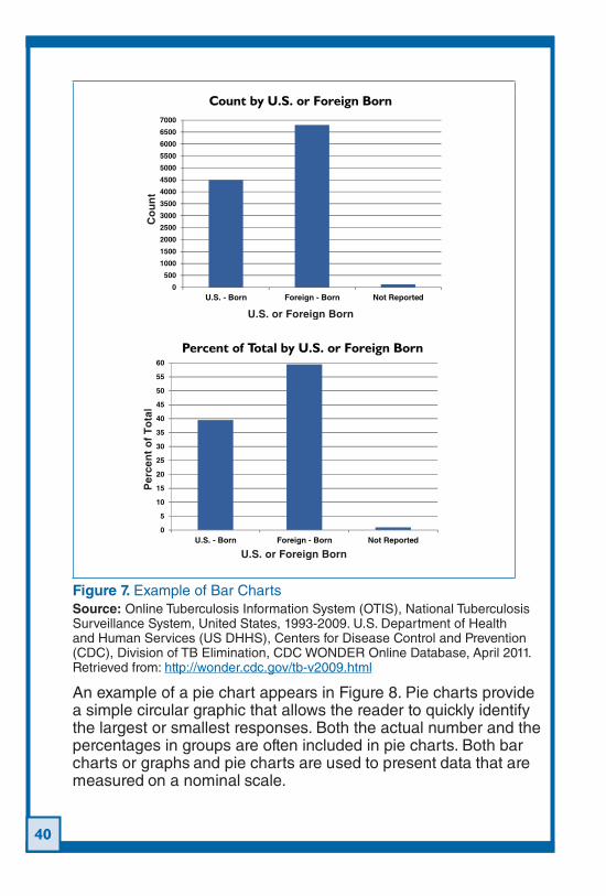
C. Presenting DataData can be graphically presented in many ways, but some of the most common methods are presented here using TB data available from the OTIS. For this first example, data on all reported TB cases by place of birth for the year 2009 was requested. Table 8 presents the counts or number of cases for each group and the percentage of the total. In 2009, 6,864 TB cases were reported in those who were foreign born. This represented 59.37% of all TB cases in the United States.
Table 8. TB Cases in the United States by Place of Birth, 2009
US or Foreign Born Count Percent of TotalUS born 4,571 39.59%Foreign born 6,854 59.37%Not reported 120 1.04%Total 11,545 100.00%
Source: Online Tuberculosis Information System (OTIS), National Tuberculosis Surveillance System, United States, 1993-2009. U.S. Department of Health and Human Services (US DHHS), Centers for Disease Control and Prevention (CDC), Division of TB Elimination, CDC WONDER Online Database, April 2011. Retrieved from: http://wonder.cdc.gov/tb-v2009.html
i. Bar Charts or Graphs and Pie ChartsThe variable “US or Foreign Born” is measured on a nominal scale. In other words, it is a variable that classifies individuals, but there is no order to this information and it is non-numeric data. The variable simply describes whether a TB case was born in the United States. The two most common ways to graphically present this type of nominal data are by using bar charts or graphs and pie charts. The vertical or Y-axis of a bar chart may present the percentage (%) of cases or the actual number of cases (as appears in Figure 7).
40
Count by U.S. or Foreign Born
0
500
1000
1500
2000
2500
3000
3500
4000
4500
5000
5500
6000
6500
7000
U.S. - Born Foreign - Born Not Reported
Co
un
t
U.S. or Foreign Born
0
5
10
15
20
25
30
35
40
45
50
55
60
U.S. - Born Foreign - Born Not Reported
Percent of Total by U.S. or Foreign Born
Per
cen
t o
f T
ota
l
U.S. or Foreign Born
Figure 7. Example of Bar ChartsSource: Online Tuberculosis Information System (OTIS), National Tuberculosis Surveillance System, United States, 1993-2009. U.S. Department of Health and Human Services (US DHHS), Centers for Disease Control and Prevention (CDC), Division of TB Elimination, CDC WONDER Online Database, April 2011. Retrieved from: http://wonder.cdc.gov/tb-v2009.html
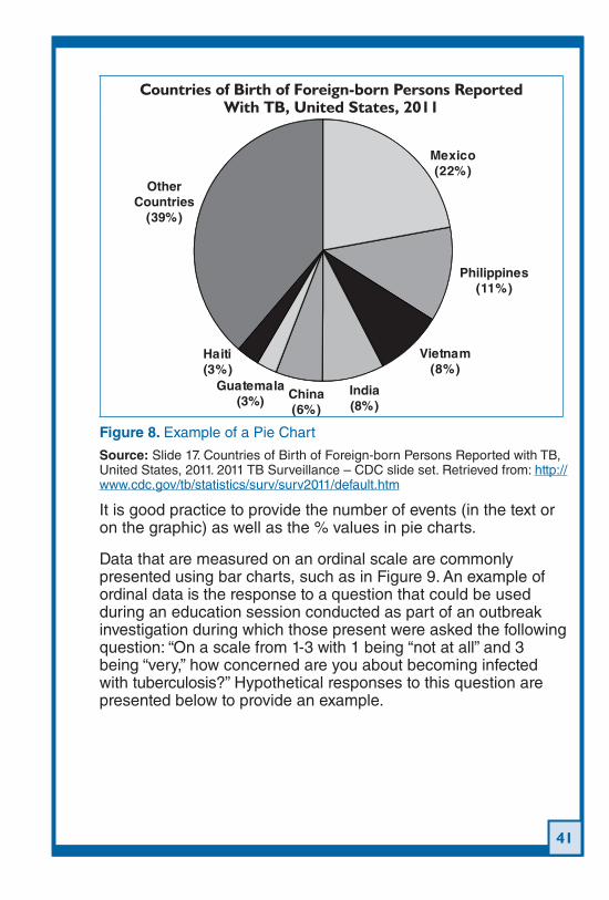
An example of a pie chart appears in Figure 8. Pie charts provide a simple circular graphic that allows the reader to quickly identify the largest or smallest responses. Both the actual number and the percentages in groups are often included in pie charts. Both bar charts or graphs and pie charts are used to present data that are measured on a nominal scale.
41
Countries of Birth of Foreign-born Persons Reported With TB, United States, 2011
Mexico(22%)
Philippines(11%)
India(8%)
Vietnam(8%)
China(6%)
Guatemala(3%)
Haiti(3%)
OtherCountries
(39%)
Figure 8. Example of a Pie Chart
Source: Slide 17. Countries of Birth of Foreign-born Persons Reported with TB, United States, 2011. 2011 TB Surveillance – CDC slide set. Retrieved from: http://www.cdc.gov/tb/statistics/surv/surv2011/default.htm
It is good practice to provide the number of events (in the text or on the graphic) as well as the % values in pie charts.
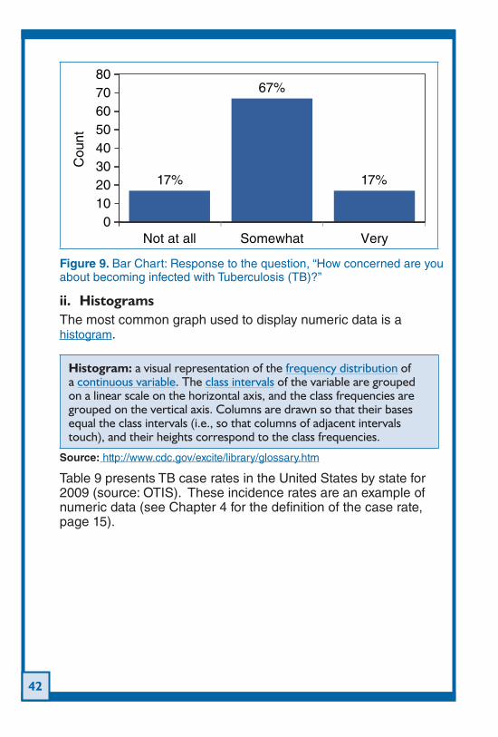
Data that are measured on an ordinal scale are commonly presented using bar charts, such as in Figure 9. An example of ordinal data is the response to a question that could be used during an education session conducted as part of an outbreak investigation during which those present were asked the following question: “On a scale from 1-3 with 1 being “not at all” and 3 being “very,” how concerned are you about becoming infected with tuberculosis?” Hypothetical responses to this question are presented below to provide an example.
42
17%
67%
17%
01020304050607080
Not at all Somewhat Very
Cou
nt
Figure 9. Bar Chart: Response to the question, “How concerned are you about becoming infected with Tuberculosis (TB)?”
ii. HistogramsThe most common graph used to display numeric data is a histogram.
Histogram: a visual representation of the frequency distribution of a continuous variable. The class intervals of the variable are grouped on a linear scale on the horizontal axis, and the class frequencies are grouped on the vertical axis. Columns are drawn so that their bases equal the class intervals (i.e., so that columns of adjacent intervals touch), and their heights correspond to the class frequencies.
Source: http://www.cdc.gov/excite/library/glossary.htm
Table 9 presents TB case rates in the United States by state for 2009 (source: OTIS). These incidence rates are an example of numeric data (see Chapter 4 for the definition of the case rate, page 15).
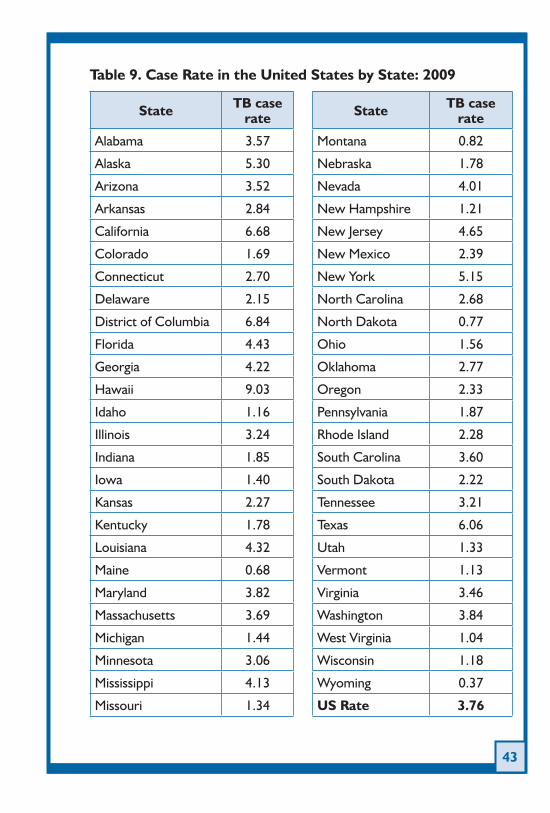
43
Table 9. Case Rate in the United States by State: 2009
State TB case rate State TB case
rate
Alabama 3.57 Montana 0.82
Alaska 5.30 Nebraska 1.78
Arizona 3.52 Nevada 4.01
Arkansas 2.84 New Hampshire 1.21
California 6.68 New Jersey 4.65
Colorado 1.69 New Mexico 2.39
Connecticut 2.70 New York 5.15
Delaware 2.15 North Carolina 2.68
District of Columbia 6.84 North Dakota 0.77
Florida 4.43 Ohio 1.56
Georgia 4.22 Oklahoma 2.77
Hawaii 9.03 Oregon 2.33
Idaho 1.16 Pennsylvania 1.87
Illinois 3.24 Rhode Island 2.28
Indiana 1.85 South Carolina 3.60
Iowa 1.40 South Dakota 2.22
Kansas 2.27 Tennessee 3.21
Kentucky 1.78 Texas 6.06
Louisiana 4.32 Utah 1.33
Maine 0.68 Vermont 1.13
Maryland 3.82 Virginia 3.46
Massachusetts 3.69 Washington 3.84
Michigan 1.44 West Virginia 1.04
Minnesota 3.06 Wisconsin 1.18
Mississippi 4.13 Wyoming 0.37
Missouri 1.34 US Rate 3.76
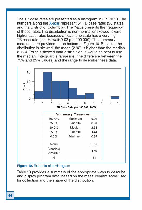
44
The TB case rates are presented as a histogram in Figure 10. The numbers along the X-axis represent 51 TB case rates (50 states and the District of Columbia). The Y-axis presents the frequency of these rates. The distribution is non-normal or skewed toward higher case rates because at least one state has a very high TB case rate (i.e., Hawaii: 9.03 per 100,000). The summary measures are provided at the bottom of Figure 10. Because the distribution is skewed, the mean (2.92) is higher than the median (2.68). For this skewed data distribution, it would be best to use the median, interquartile range (i.e., the difference between the 75% and 25% values) and the range to describe these data.
Co
un
t
5
15
0 1 2 3 4 5 6 7 8 9 10
10
0
TB Case Rate per 100,000 2009
Summary Measures100.0% Maximum 9.0375.0% Quartile 3.8450.0% Median 2.6825.0% Quartile 1.440.0% Minimum 0.37
Mean 2.925
Standard Deviation
1.79
N 51
Figure 10. Example of a Histogram
Table 10 provides a summary of the appropriate ways to describe and display program data, based on the measurement scale used for collection and the shape of the distribution.
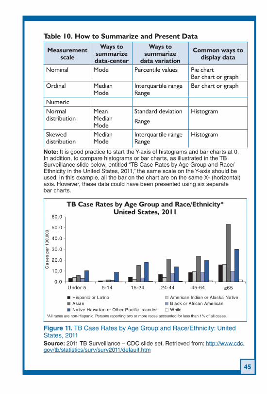
45
Table 10. How to Summarize and Present Data
Measurement scale
Ways to summarize data-center
Ways to summarize
data variation
Common ways to display data
Nominal Mode Percentile values Pie chart Bar chart or graph
Ordinal Median Mode
Interquartile range Range
Bar chart or graph
NumericNormal distribution
Mean Median Mode
Standard deviation
Range
Histogram
Skewed distribution
Median Mode
Interquartile range Range
Histogram
Note: It is good practice to start the Y-axis of histograms and bar charts at 0. In addition, to compare histograms or bar charts, as illustrated in the TB Surveillance slide below, entitled “TB Case Rates by Age Group and Race/Ethnicity in the United States, 2011,” the same scale on the Y-axis should be used. In this example, all the bar on the chart are on the same X- (horizontal) axis. However, these data could have been presented using six separate bar charts.
TB Case Rates by Age Group and Race/Ethnicity* United States, 2011
Ca
se
s p
er
10
0,0
00
0.0
10.0
20.0
30.0
40.0
50.0
60.0
Under 5 5-14 15-24 24-44 45-64 ≥65
Hispanic or Latino American Indian or Alaska NativeAsian B lack or African AmericanNative Hawaiian or Other Pacific Is lander White
*All races are non-Hispanic. Persons reporting two or more races accounted for less than 1% of all cases.
Figure 11. TB Case Rates by Age Group and Race/Ethnicity: United States, 2011Source: 2011 TB Surveillance – CDC slide set. Retrieved from: http://www.cdc.gov/tb/statistics/surv/surv2011/default.htm
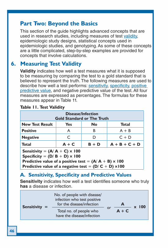
46
Part Two: Beyond the BasicsThis section of the guide highlights advanced concepts that are used in research studies, including measures of test validity, epidemiologic study designs, statistical concepts used in epidemiologic studies, and genotyping. As some of these concepts are a little complicated, step-by-step examples are provided for concepts that involve calculations.
Measuring Test Validity6. Validity indicates how well a test measures what it is supposed to be measuring by comparing the test to a gold standard that is believed to represent the truth. The following measures are used to describe how well a test performs: sensitivity, specificity, positive predictive value, and negative predictive value of the test. All four measures are expressed as percentages. The formulas for these measures appear in Table 11.
Table 11. Test ValidityDisease/Infection
Gold Standard or The TruthNew Test Result Yes No TotalPositive A B A + B
Negative C D C + D
Total A + C B + D A + B + C + D
Sensitivity = (A/ A + C) × 100Specificity = (D/ B + D) × 100Predictive value of a positive test = (A/ A + B) × 100Predictive value of a negative test = (D/ C + D) ×100
A. Sensitivity, Specificity and Predictive ValuesSensitivity indicates how well a test identifies someone who truly has a disease or infection.
Sensitivity =
No. of people with disease/ infection who test positive for the disease/infection
or
A
x 100Total no. of people who
have the disease/infectionA + C
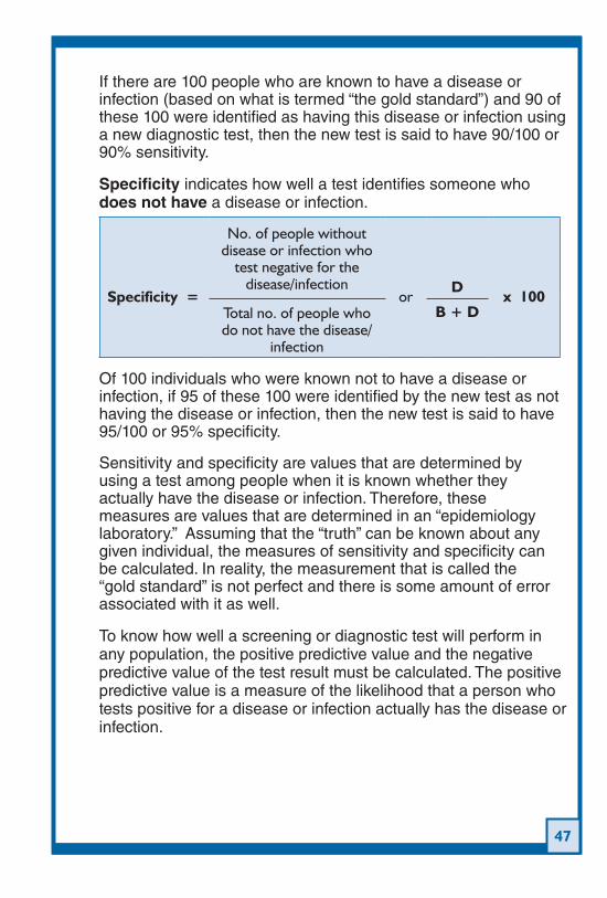
47
If there are 100 people who are known to have a disease or infection (based on what is termed “the gold standard”) and 90 of these 100 were identified as having this disease or infection using a new diagnostic test, then the new test is said to have 90/100 or 90% sensitivity.
Specificity indicates how well a test identifies someone who does not have a disease or infection.
Specificity =
No. of people without disease or infection who
test negative for the disease/infection
or
D x 100
Total no. of people who do not have the disease/
infection
B + D
Of 100 individuals who were known not to have a disease or infection, if 95 of these 100 were identified by the new test as not having the disease or infection, then the new test is said to have 95/100 or 95% specificity.
Sensitivity and specificity are values that are determined by using a test among people when it is known whether they actually have the disease or infection. Therefore, these measures are values that are determined in an “epidemiology laboratory.” Assuming that the “truth” can be known about any given individual, the measures of sensitivity and specificity can be calculated. In reality, the measurement that is called the “gold standard” is not perfect and there is some amount of error associated with it as well.
To know how well a screening or diagnostic test will perform in any population, the positive predictive value and the negative predictive value of the test result must be calculated. The positive predictive value is a measure of the likelihood that a person who tests positive for a disease or infection actually has the disease or infection.
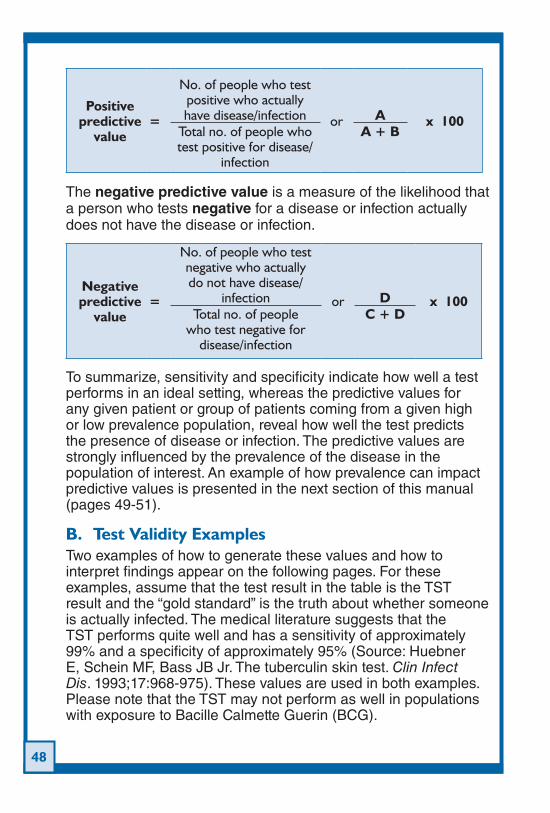
48
Positive predictive
value=
No. of people who test positive who actually have disease/infection or
A x 100
Total no. of people who test positive for disease/
infection
A + B
The negative predictive value is a measure of the likelihood that a person who tests negative for a disease or infection actually does not have the disease or infection.
Negative predictive
value=
No. of people who test negative who actually do not have disease/
infection or
D x 100
Total no. of people who test negative for
disease/infection
C + D
To summarize, sensitivity and specificity indicate how well a test performs in an ideal setting, whereas the predictive values for any given patient or group of patients coming from a given high or low prevalence population, reveal how well the test predicts the presence of disease or infection. The predictive values are strongly influenced by the prevalence of the disease in the population of interest. An example of how prevalence can impact predictive values is presented in the next section of this manual (pages 49-51).
B. Test Validity ExamplesTwo examples of how to generate these values and how to interpret findings appear on the following pages. For these examples, assume that the test result in the table is the TST result and the “gold standard” is the truth about whether someone is actually infected. The medical literature suggests that the TST performs quite well and has a sensitivity of approximately 99% and a specificity of approximately 95% (Source: Huebner E, Schein MF, Bass JB Jr. The tuberculin skin test. Clin Infect Dis. 1993;17:968-975). These values are used in both examples. Please note that the TST may not perform as well in populations with exposure to Bacille Calmette Guerin (BCG).
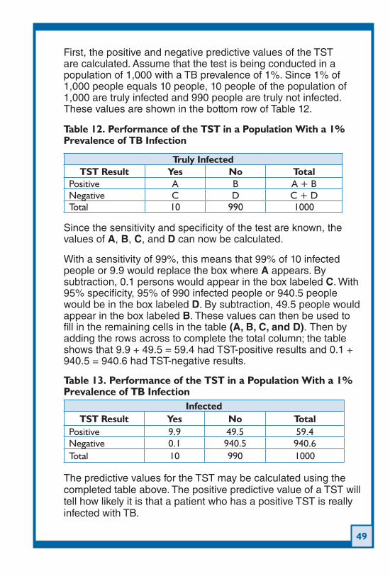
49
First, the positive and negative predictive values of the TST are calculated. Assume that the test is being conducted in a population of 1,000 with a TB prevalence of 1%. Since 1% of 1,000 people equals 10 people, 10 people of the population of 1,000 are truly infected and 990 people are truly not infected. These values are shown in the bottom row of Table 12.
Table 12. Performance of the TST in a Population With a 1% Prevalence of TB Infection
Truly InfectedTST Result Yes No Total
Positive A B A + BNegative C D C + DTotal 10 990 1000
Since the sensitivity and specificity of the test are known, the values of A, B, C, and D can now be calculated.
With a sensitivity of 99%, this means that 99% of 10 infected people or 9.9 would replace the box where A appears. By subtraction, 0.1 persons would appear in the box labeled C. With 95% specificity, 95% of 990 infected people or 940.5 people would be in the box labeled D. By subtraction, 49.5 people would appear in the box labeled B. These values can then be used to fill in the remaining cells in the table (A, B, C, and D). Then by adding the rows across to complete the total column; the table shows that 9.9 + 49.5 = 59.4 had TST-positive results and 0.1 + 940.5 = 940.6 had TST-negative results.
Table 13. Performance of the TST in a Population With a 1% Prevalence of TB Infection
InfectedTST Result Yes No Total
Positive 9.9 49.5 59.4Negative 0.1 940.5 940.6Total 10 990 1000
The predictive values for the TST may be calculated using the completed table above. The positive predictive value of a TST will tell how likely it is that a patient who has a positive TST is really infected with TB.
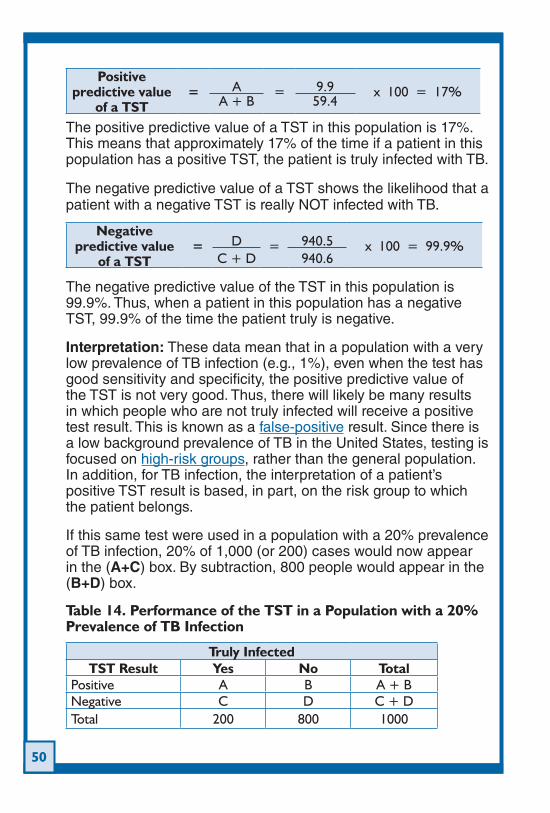
50
Positive predictive value
of a TST= A = 9.9 x 100 = 17%
A + B 59.4
The positive predictive value of a TST in this population is 17%. This means that approximately 17% of the time if a patient in this population has a positive TST, the patient is truly infected with TB.
The negative predictive value of a TST shows the likelihood that a patient with a negative TST is really NOT infected with TB.
Negative predictive value
of a TST= D = 940.5 x 100 = 99.9%
C + D 940.6
The negative predictive value of the TST in this population is 99.9%. Thus, when a patient in this population has a negative TST, 99.9% of the time the patient truly is negative.
Interpretation: These data mean that in a population with a very low prevalence of TB infection (e.g., 1%), even when the test has good sensitivity and specificity, the positive predictive value of the TST is not very good. Thus, there will likely be many results in which people who are not truly infected will receive a positive test result. This is known as a false-positive result. Since there is a low background prevalence of TB in the United States, testing is focused on high-risk groups, rather than the general population. In addition, for TB infection, the interpretation of a patient’s positive TST result is based, in part, on the risk group to which the patient belongs.
If this same test were used in a population with a 20% prevalence of TB infection, 20% of 1,000 (or 200) cases would now appear in the (A+C) box. By subtraction, 800 people would appear in the (B+D) box.
Table 14. Performance of the TST in a Population with a 20% Prevalence of TB Infection
Truly InfectedTST Result Yes No Total
Positive A B A + BNegative C D C + DTotal 200 800 1000
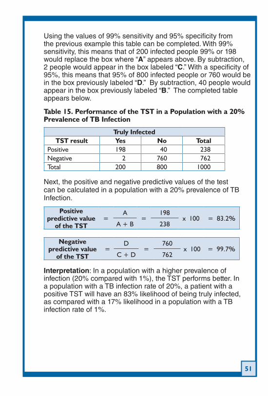
51
Using the values of 99% sensitivity and 95% specificity from the previous example this table can be completed. With 99% sensitivity, this means that of 200 infected people 99% or 198 would replace the box where “A” appears above. By subtraction, 2 people would appear in the box labeled “C.” With a specificity of 95%, this means that 95% of 800 infected people or 760 would be in the box previously labeled “D.” By subtraction, 40 people would appear in the box previously labeled “B.” The completed table appears below.
Table 15. Performance of the TST in a Population with a 20% Prevalence of TB Infection
Truly InfectedTST result Yes No Total
Positive 198 40 238Negative 2 760 762Total 200 800 1000
Next, the positive and negative predictive values of the test can be calculated in a population with a 20% prevalence of TB Infection.
Positive predictive value
of the TST=
A=
198x 100 = 83.2%
A + B 238
Negative predictive value
of the TST=
D=
760x 100 = 99.7%
C + D 762
Interpretation: In a population with a higher prevalence of infection (20% compared with 1%), the TST performs better. In a population with a TB infection rate of 20%, a patient with a positive TST will have an 83% likelihood of being truly infected, as compared with a 17% likelihood in a population with a TB infection rate of 1%.
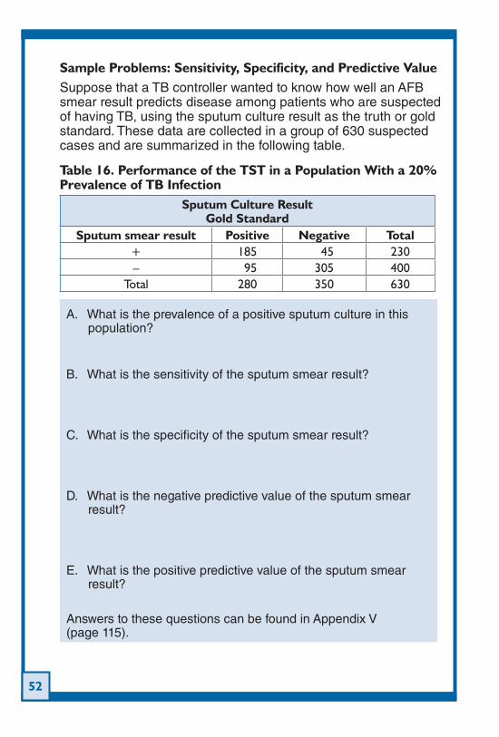
52
Sample Problems: Sensitivity, Specificity, and Predictive ValueSuppose that a TB controller wanted to know how well an AFB smear result predicts disease among patients who are suspected of having TB, using the sputum culture result as the truth or gold standard. These data are collected in a group of 630 suspected cases and are summarized in the following table.
Table 16. Performance of the TST in a Population With a 20% Prevalence of TB Infection
Sputum Culture Result Gold Standard
Sputum smear result Positive Negative Total+ 185 45 230– 95 305 400
Total 280 350 630
A. What is the prevalence of a positive sputum culture in this population?
B. What is the sensitivity of the sputum smear result?
C. What is the specificity of the sputum smear result?
D. What is the negative predictive value of the sputum smear result?
E. What is the positive predictive value of the sputum smear result?
Answers to these questions can be found in Appendix V (page 115).
53
Study Designs7. There are four types of epidemiologic studies that appear most frequently in the medical and public health literature: cross-sectional studies, case-control studies, cohort studies, and clinical trials.
A. Cross-Sectional Studies
Study design, cross-sectional – a study in which a sample of persons from a population is enrolled and their exposures and health outcomes are measured simultaneously; a survey.
Source: http://www.cdc.gov/excite/library/glossary.htm
Cross-sectional studies provide information on possible risk factors and disease outcomes at the same point in time. They are sometimes called prevalence studies since they can provide prevalence measures. The data collected present a picture of what is occurring at a specific time. Cross-sectional studies cannot provide information on causes of diseases since it is unclear in these studies whether the disease or the supposed risk factor occurred first. Cross-sectional studies are usually descriptive, in that they describe the disease or condition in a population at a given time, in terms of person, place, and time. The following excerpt provides an example of a cross-sectional or prevalence study.
Study Design: Cross-Sectional Study“Objective: To determine the prevalence of and risk factors for tuberculin skin test positivity and conversion among New York City Department of Health and Mental Hygiene employees.
Design: Point-prevalence survey. Sentinel surveillance was conducted from March 1, 1994 to December 31, 2001.
Participants: HCWs in high-risk and low-risk settings for occupational TB exposure.
Results: Baseline tuberculin positivity was 36.2% (600 of 1,658), 15.5% (143 of 922) among HCWs born in the United States, and 48.5% (182 of 375) among HCWs not born in the United States.”
Source: Cook S, Maw KL, Munsiff SS, Fujiwara PI, Frieden TR. Prevalence of tuberculin skin test positivity and conversions among healthcare workers in New York City during 1994 to 2001. Infect Control Hosp Epidemiol. 2003;24:807-813. Reprinted here with permission.
54
B. Case-Control StudiesCase-control studies are a type of analytic epidemiologic study that allows the researchers to estimate the strength of the association between the disease and a particular risk factor. Cases are people with disease or infection, whereas controls do not have the disease or infection. Once the cases and controls are identified, they are questioned about potential risk factors that occurred in their past. Case-control studies are especially useful when the disease outcome being studied is rare, since in an observational study of a rare event, only a few cases might ever be identified.
Study Design: Case-Control StudyAn observational analytic study that enrolls one group of persons with a certain disease, chronic condition, or type of injury (case-patients) and a group of persons without the health problem (control subjects) and compares differences in exposures, behaviors, and other characteristics to identify and quantify associations, test hypotheses, and identify causes.
Source: http://www.cdc.gov/excite/library/glossary.htm
An excerpt of an abstract from a case-control study follows.
Study Design: Case-Control“Background:Successful treatment of tuberculosis (TB) involves taking anti-tuberculosis drugs for at least six months. Poor adherence to treatment means patients remain infectious for longer, are more likely to relapse or succumb to tuberculosis and could result in treatment failure as well as foster emergence of drug resistant tuberculosis. Kenya is among countries with high tuberculosis burden globally. The purpose of this study was to determine the duration tuberculosis patients stay in treatment before defaulting and factors associated with default in Nairobi.
Methods:A Case-Control study; Cases were those who defaulted from treatment and Controls those who completed treatment course between January 2006 and March 2008. All (945) defaulters and 1033 randomly selected controls from among 5659 patients who completed treatment course in 30 high volume sites were enrolled. Secondary data was collected using a facility questionnaire. From among the enrolled, 120 cases and 154 controls were randomly selected and interviewed to obtain primary data not routinely collected.”
Source: Muture BN, Keraka MN, Kimuu PK, Kabiru EW, Ombeka VO, Oguya F. Factors associated with default from treatment among tuberculosis patients in Nairobi province, Kenya: A case control study. BMC Public Health. 2011;11:696.
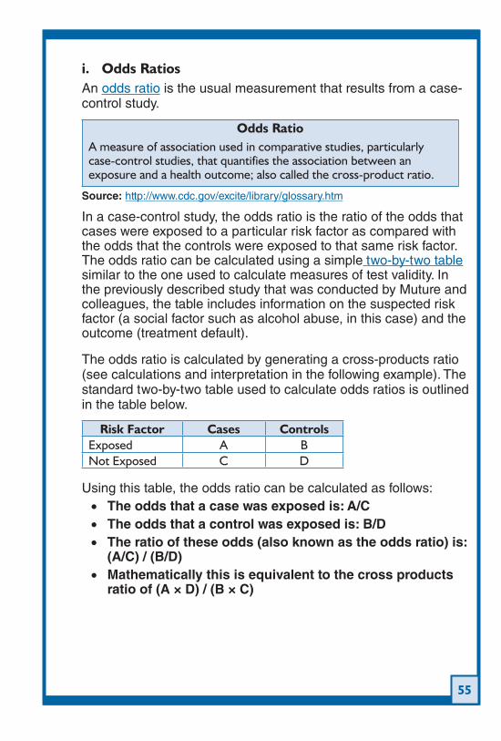
55
i. Odds RatiosAn odds ratio is the usual measurement that results from a case-control study.
Odds RatioA measure of association used in comparative studies, particularly case-control studies, that quantifies the association between an exposure and a health outcome; also called the cross-product ratio.
Source: http://www.cdc.gov/excite/library/glossary.htm
In a case-control study, the odds ratio is the ratio of the odds that cases were exposed to a particular risk factor as compared with the odds that the controls were exposed to that same risk factor. The odds ratio can be calculated using a simple two-by-two table similar to the one used to calculate measures of test validity. In the previously described study that was conducted by Muture and colleagues, the table includes information on the suspected risk factor (a social factor such as alcohol abuse, in this case) and the outcome (treatment default).
The odds ratio is calculated by generating a cross-products ratio (see calculations and interpretation in the following example). The standard two-by-two table used to calculate odds ratios is outlined in the table below.
Risk Factor Cases ControlsExposed A BNot Exposed C D
Using this table, the odds ratio can be calculated as follows:The odds that a case was exposed is: A/C•The odds that a control was exposed is: B/D•The ratio of these odds (also known as the odds ratio) is: •(A/C) / (B/D)Mathematically this is equivalent to the cross products •ratio of (A × D) / (B × C)
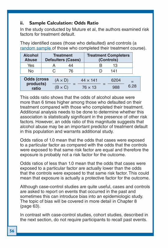
56
ii. Sample Calculation: Odds RatioIn the study conducted by Muture et al, the authors examined risk factors for treatment default.
They identified cases (those who defaulted) and controls (a random sample of those who completed their treatment course).
Alcohol Abuse
Treatment Defaulters (Cases)
Treatment Completers (Controls)
Yes A 44 B 13No C 76 D 141
Odds (cross products)
ratio
(A × D)=
44 × 141=
6204 = 6.28(B × C) 76 × 13 988
This odds ratio shows that the odds of alcohol abuse were more than 6 times higher among those who defaulted on their treatment compared with those who completed their treatment. Additional analysis needs to be done to determine whether this association is statistically significant in the presence of other risk factors. However, an odds ratio of this magnitude suggests that alcohol abuse may be an important predictor of treatment default in this population and warrants additional study.
Odds ratios of 1.0 mean that the odds that cases were exposed to a particular factor as compared with the odds that the controls were exposed to that same risk factor are equal and therefore the exposure is probably not a risk factor for the outcome.
Odds ratios of less than 1.0 mean that the odds that cases were exposed to a particular factor are actually lower than the odds that the controls were exposed to that same risk factor. This could mean that exposure is actually a protective factor for the outcome.
Although case-control studies are quite useful, cases and controls are asked to report on events that occurred in the past and sometimes this can introduce bias into an epidemiologic study. The topic of bias will be covered in more detail in Chapter 8 (page 63).
In contrast with case-control studies, cohort studies, described in the next section, do not require participants to recall past events.
57
C. Cohort StudiesIn a cohort study, researchers collect information on a group of exposed and unexposed individuals over time and then calculate incidence rates. These incidence rates allow for the direct calculation of a measure of association between a risk factor and an outcome, called the relative risk.
Study Design: Cohort StudyAn observational analytic study in which enrollment is based on status of exposure o a certain factor or membership in a certain group. Populations are followed, and disease, death, or other health-related outcomes are documented and compared.
Source: http://www.cdc.gov/excite/library/glossary.htm
Cohort studies, as compared with cross-sectional and case-control studies, provide the most useful epidemiologic measures (incidence rates), but, in general, they take the longest to complete and are more costly and labor intensive. In addition, some participants will fail to complete the study and this loss (known as loss to follow-up) could bias the results of the study.
Sometimes cohort studies are conducted in populations in which all the activities have occurred in the past. These are called historical cohort studies. What distinguishes them as cohort studies is that the group members are organized by their exposure status at the beginning of the study and then information on their outcomes is collected to compare the group outcomes.
i. Relative RiskThe relative risk (RR) is sometimes called a rate ratio or risk ratio.
Risk Ratio (RR)A measure of association that quantifies the association between an exposure and a health outcome from an epidemiologic study, calculated as the ratio of incidence proportions of two groups
Source: http://www.cdc.gov/excite/library/glossary.htm
Relative risk =Incidence rate in the group exposed to the
risk factorIncidence rate in the unexposed group
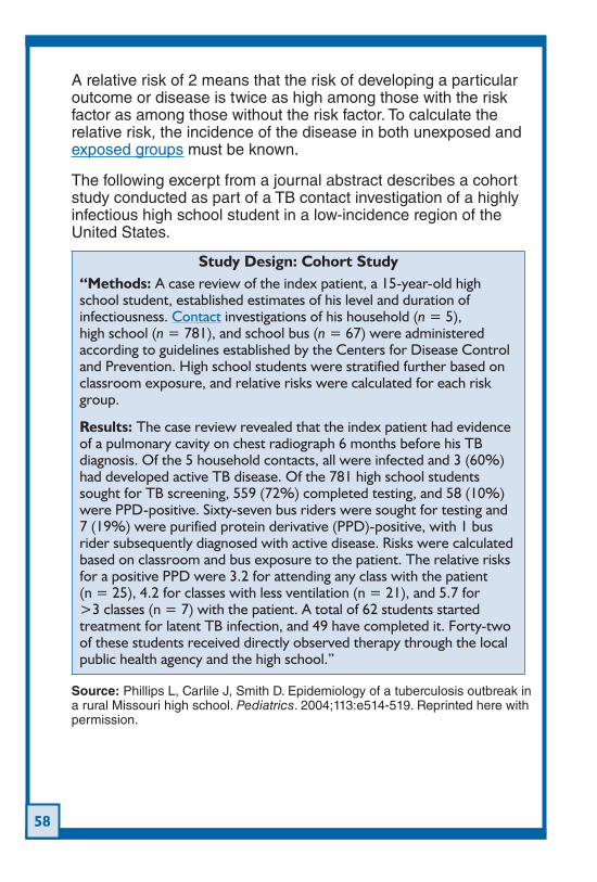
58
A relative risk of 2 means that the risk of developing a particular outcome or disease is twice as high among those with the risk factor as among those without the risk factor. To calculate the relative risk, the incidence of the disease in both unexposed and exposed groups must be known.
The following excerpt from a journal abstract describes a cohort study conducted as part of a TB contact investigation of a highly infectious high school student in a low-incidence region of the United States.
Study Design: Cohort Study“Methods: A case review of the index patient, a 15-year-old high school student, established estimates of his level and duration of infectiousness. Contact investigations of his household (n = 5), high school (n = 781), and school bus (n = 67) were administered according to guidelines established by the Centers for Disease Control and Prevention. High school students were stratified further based on classroom exposure, and relative risks were calculated for each risk group.
Results: The case review revealed that the index patient had evidence of a pulmonary cavity on chest radiograph 6 months before his TB diagnosis. Of the 5 household contacts, all were infected and 3 (60%) had developed active TB disease. Of the 781 high school students sought for TB screening, 559 (72%) completed testing, and 58 (10%) were PPD-positive. Sixty-seven bus riders were sought for testing and 7 (19%) were purified protein derivative (PPD)-positive, with 1 bus rider subsequently diagnosed with active disease. Risks were calculated based on classroom and bus exposure to the patient. The relative risks for a positive PPD were 3.2 for attending any class with the patient (n = 25), 4.2 for classes with less ventilation (n = 21), and 5.7 for >3 classes (n = 7) with the patient. A total of 62 students started treatment for latent TB infection, and 49 have completed it. Forty-two of these students received directly observed therapy through the local public health agency and the high school.”
Source: Phillips L, Carlile J, Smith D. Epidemiology of a tuberculosis outbreak in a rural Missouri high school. Pediatrics. 2004;113:e514-519. Reprinted here with permission.
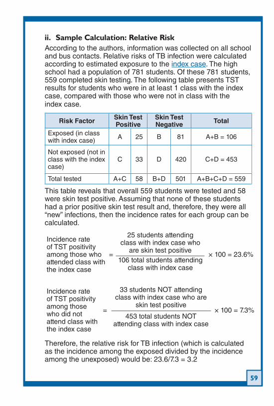
59
ii. Sample Calculation: Relative RiskAccording to the authors, information was collected on all school and bus contacts. Relative risks of TB infection were calculated according to estimated exposure to the index case. The high school had a population of 781 students. Of these 781 students, 559 completed skin testing. The following table presents TST results for students who were in at least 1 class with the index case, compared with those who were not in class with the index case.
Risk Factor Skin Test Positive
Skin Test Negative Total
Exposed (in class with index case) A 25 B 81 A+B = 106
Not exposed (not in class with the index case)
C 33 D 420 C+D = 453
Total tested A+C 58 B+D 501 A+B+C+D = 559
This table reveals that overall 559 students were tested and 58 were skin test positive. Assuming that none of these students had a prior positive skin test result and, therefore, they were all “new” infections, then the incidence rates for each group can be calculated.
Incidence rate of TST positivity among those who attended class with the index case
=
25 students attending class with index case who
are skin test positive × 100 = 23.6%
106 total students attending class with index case
Incidence rate of TST positivity among those who did not attend class with the index case
=
33 students NOT attending class with index case who are
skin test positive × 100 = 7.3%
453 total students NOT attending class with index case
Therefore, the relative risk for TB infection (which is calculated as the incidence among the exposed divided by the incidence among the unexposed) would be: 23.6/7.3 = 3.2
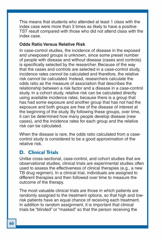
60
This means that students who attended at least 1 class with the index case were more than 3 times as likely to have a positive TST result compared with those who did not attend class with the index case.
Odds Ratio Versus Relative RiskIn case-control studies, the incidence of disease in the exposed and unexposed groups is unknown, since some preset number of people with disease and without disease (cases and controls) is specifically selected by the researcher. Because of the way that the cases and controls are selected in a case-control study, incidence rates cannot be calculated and therefore, the relative risk cannot be calculated. Instead, researchers calculate the odds ratio as the measure of association that describes the relationship between a risk factor and a disease in a case-control study. In a cohort study, relative risk can be calculated directly using available incidence rates, because there is a group that has had some exposure and another group that has not had the exposure and both groups are free of the disease of interest at the beginning of the study. By following these groups, over time, it can be determined how many people develop disease (new cases), and the incidence rates for each group and the relative risk can be calculated.
When the disease is rare, the odds ratio calculated from a case-control study is considered to be a good approximation of the relative risk.
D. Clinical TrialsUnlike cross-sectional, case-control, and cohort studies that are observational studies, clinical trials are experimental studies often used to assess the effectiveness of clinical therapies (e.g., a new TB drug regimen). In a clinical trial, individuals are assigned to different therapies and then followed over time to measure the outcome of the therapy.
The most valuable clinical trials are those in which patients are randomly assigned to the treatment options, so that high and low-risk patients have an equal chance of receiving each treatment. In addition to random assignment, it is important that clinical trials be “blinded” or “masked” so that the person receiving the
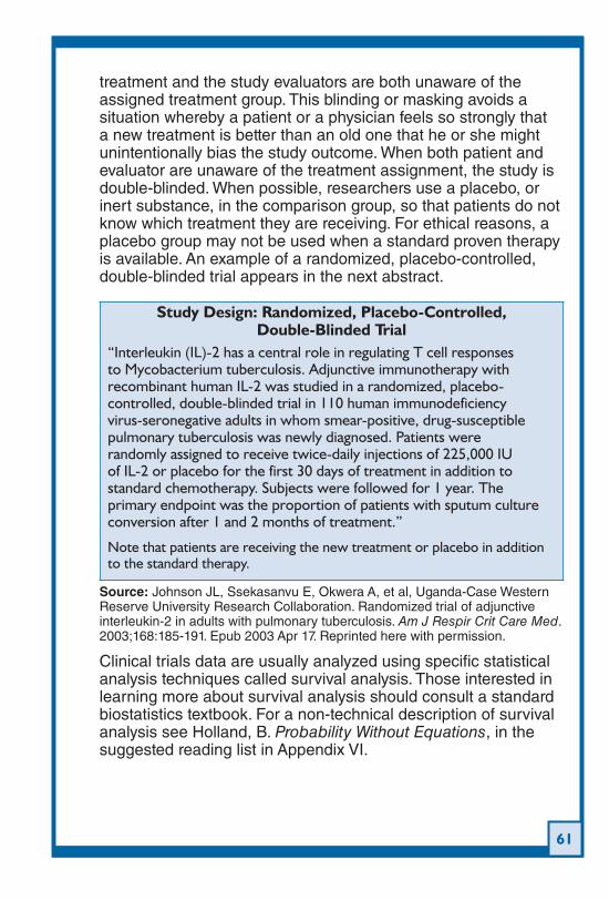
61
treatment and the study evaluators are both unaware of the assigned treatment group. This blinding or masking avoids a situation whereby a patient or a physician feels so strongly that a new treatment is better than an old one that he or she might unintentionally bias the study outcome. When both patient and evaluator are unaware of the treatment assignment, the study is double-blinded. When possible, researchers use a placebo, or inert substance, in the comparison group, so that patients do not know which treatment they are receiving. For ethical reasons, a placebo group may not be used when a standard proven therapy is available. An example of a randomized, placebo-controlled, double-blinded trial appears in the next abstract.
Study Design: Randomized, Placebo-Controlled, Double-Blinded Trial
“Interleukin (IL)-2 has a central role in regulating T cell responses to Mycobacterium tuberculosis. Adjunctive immunotherapy with recombinant human IL-2 was studied in a randomized, placebo-controlled, double-blinded trial in 110 human immunodeficiency virus-seronegative adults in whom smear-positive, drug-susceptible pulmonary tuberculosis was newly diagnosed. Patients were randomly assigned to receive twice-daily injections of 225,000 IU of IL-2 or placebo for the first 30 days of treatment in addition to standard chemotherapy. Subjects were followed for 1 year. The primary endpoint was the proportion of patients with sputum culture conversion after 1 and 2 months of treatment.”
Note that patients are receiving the new treatment or placebo in addition to the standard therapy.
Source: Johnson JL, Ssekasanvu E, Okwera A, et al, Uganda-Case Western Reserve University Research Collaboration. Randomized trial of adjunctive interleukin-2 in adults with pulmonary tuberculosis. Am J Respir Crit Care Med. 2003;168:185-191. Epub 2003 Apr 17. Reprinted here with permission.
Clinical trials data are usually analyzed using specific statistical analysis techniques called survival analysis. Those interested in learning more about survival analysis should consult a standard biostatistics textbook. For a non-technical description of survival analysis see Holland, B. Probability Without Equations, in the suggested reading list in Appendix VI.
62
Study Design Take Home Points:Cross-Sectional Studies provide a snap shot of the health status of a group at one particular time. They are usually quicker and less expensive than other study designs. They can be used to generate hypotheses regarding risk factors and disease outcome, but they cannot be used to support a causal association. The measurement most often produced is prevalence.
Case-Control Studies take less time and are less expensive than cohort studies. They are particularly good when the outcome being studied is rare. The study design requires that participants recall exposure to particular risk factors. Therefore, the measure of association may be affected by faulty or biased recall. The measurement most often produced is an odds ratio, which is an estimate of relative risk.
Cohort Studies are the most expensive and time consuming of all epidemiologic studies, but they produce incidence rates and relative risks. Cohort studies are observational, whereby a researcher observes a group over time. Since individuals are studied over longer periods of time, compared with case-control or cross-sectional studies, some people may drop out of the study, which may bias the incidence rates and relative risk.
Clinical Trials are experimental studies used to assess treatment effectiveness. The best trials are usually those that are randomized, placebo-controlled, and double-blinded.
63
Statistical Concepts Used in Epidemiologic 8. StudiesWhen reading articles and assessing epidemiologic studies in journals, it is important to understand how these results are evaluated as statistically significant or not significant. The tools that epidemiologists often use to evaluate the statistical significance of research findings include p-values and confidence intervals. In addition, when evaluating the results of studies, issues of possible confounding factors and bias must also be considered. Sometimes the results of a number of studies are combined in a meta-analysis to assess the full weight of the evidence provided in the clinical and public health literature. Each of these five topics is described briefly in this chapter. Those interested in more detailed explanations will find these topics in most basic text books on biostatistics and epidemiology.
A. P-ValuesWhen testing a hypothesis or research question, the researcher must decide how sure he or she wishes to be about the study results, prior to conducting the study. This is done by choosing a significance or risk level (called the alpha level). The most common significance levels used by researchers are .05 and .01. The alpha level represents the risk that the researcher is willing to accept that any differences found are due to chance alone. If a test is conducted at the alpha = 0.05 level, it is accepted that 5 of 100 times or 5% of the time something might be found to be statistically significant when the result actually occurred by chance. If a test is conducted at the alpha = 0.01 level, then the researcher is being more averse to the risk of falsely reporting a significant finding, so that 1 out of 100 times or only 1% of the time, this result will be due to chance alone. Once the statistical test is completed, the p-value, generated by a statistical software package, is compared to the preset alpha level. If the p-value is smaller than the alpha level, then the result is said to be statistically significant and unlikely to be due to chance alone.
64
B. Confidence IntervalsIncidence rates, prevalence measures, odds ratios, and relative risks are often presented with confidence intervals (often the abbreviation CI is used). Usually 95% confidence intervals are reported in the medical literature. A confidence interval tells the reader how confident researchers are that the sample value (i.e., the prevalence or incidence estimate or the odds ratio or relative risk) represents the population from which it was taken. When confidence intervals are calculated, they take into account the size of the sample and the amount of variability there is around the measurement.
95% Confidence Intervals on Incidence and Prevalence Measures
When confidence intervals are reported for incidence or prevalence measures researchers are usually presenting an estimated value that they have calculated from a smaller sample to learn more about what is happening in a larger population. In these cases, they want to provide the reader with some estimate of the amount of variability that can be expected around the estimate. The 95% confidence interval establishes that there is 95% certainty that the true population value falls within that interval. For example in an article in the Bulletin of the World Health Organization, Guwatudde and colleagues reported that they found a prevalence for all forms of TB of 14.0 per thousand with a 95% confidence interval (CI) of 7.8–20.3 in Kampala, Uganda. These data tell the reader that based on the results of their study, they are 95% sure that the true prevalence of all forms of TB in Kampala, Uganda, falls somewhere between 7.8 and 20.3 per 1000 population. To have a narrower confidence interval, these researchers could have increased the size of their sample.
Source: Guwatudde D, Zalwango S, Kamya MR, Debanne SM, Diaz MI, Okwera A, Mugerwa RD, King C, Whalen CC. Burden of tuberculosis in Kampala, Uganda. Bull World Health Org. 2003, 81(11):799-805.
95% Confidence Intervals on Odds Ratios and Relative Risks
95% confidence intervals on risk estimates such as odds ratios and relative risks also provide an estimate of variability around these measures. If the 95% confidence interval on an odds ratio or a relative risk includes the number 1.0, this means that the
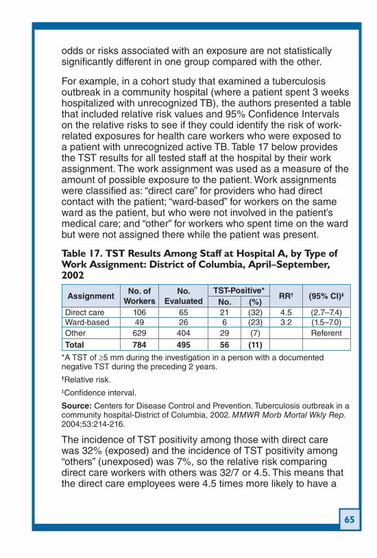
65
odds or risks associated with an exposure are not statistically significantly different in one group compared with the other.
For example, in a cohort study that examined a tuberculosis outbreak in a community hospital (where a patient spent 3 weeks hospitalized with unrecognized TB), the authors presented a table that included relative risk values and 95% Confidence Intervals on the relative risks to see if they could identify the risk of work-related exposures for health care workers who were exposed to a patient with unrecognized active TB. Table 17 below provides the TST results for all tested staff at the hospital by their work assignment. The work assignment was used as a measure of the amount of possible exposure to the patient. Work assignments were classified as: “direct care” for providers who had direct contact with the patient; “ward-based” for workers on the same ward as the patient, but who were not involved in the patient’s medical care; and “other” for workers who spent time on the ward but were not assigned there while the patient was present.
Table 17. TST Results Among Staff at Hospital A, by Type of Work Assignment: District of Columbia, April–September, 2002
AssignmentNo. of
WorkersNo.
EvaluatedTST-Positive*
RR† (95% CI)‡
No. (%)Direct care 106 65 21 (32) 4.5 (2.7–7.4)Ward-based 49 26 6 (23) 3.2 (1.5–7.0)Other 629 404 29 (7) ReferentTotal 784 495 56 (11)
*A TST of ≥5 mm during the investigation in a person with a documented negative TST during the preceding 2 years.†Relative risk.‡Confidence interval.
Source: Centers for Disease Control and Prevention. Tuberculosis outbreak in a community hospital-District of Columbia, 2002. MMWR Morb Mortal Wkly Rep. 2004;53:214-216.
The incidence of TST positivity among those with direct care was 32% (exposed) and the incidence of TST positivity among “others” (unexposed) was 7%, so the relative risk comparing direct care workers with others was 32/7 or 4.5. This means that the direct care employees were 4.5 times more likely to have a
66
positive TST result compared with those described as “other” employees. In this example the “other” group is considered to be the “referent” or comparison group.
The 95% confidence intervals, which appear in the final column of the table, provide an estimate of how much variation might be expected for this estimate of relative risk. The 95% confidence interval for the relative risk of 4.5 is 2.7-7.4, meaning that the estimate of increased risk for those in the “direct care” group could vary from a lower value of 2.7 times higher up to a high value of 7.4 times higher than the risk among the “others”. The endpoints, which define the confidence interval (in this case 2.7 and 7.4) are also called confidence limits.
This table presents a good example of how epidemiology and statistics can be used in an outbreak investigation. The relative risks and confidence intervals provide TB controllers with a meaningful estimate of where exposure occurred and this information can then be used to concentrate their efforts on testing additional at-risk workers.
C. Confounding FactorsIn epidemiologic studies, there may be other factors in addition to the risk factor being tested that will affect or confound the results. For example, if researchers use a cohort study to investigate whether men are more likely than women to develop TB disease when infected, the researchers might pick a population of 100 women and 100 men who are newly infected with TB and follow them for 10 years. However, clearly there are other factors that will affect whether a patient progresses to TB disease, such as HIV infection, age, or presence of diabetes. Statistical techniques exist to adjust for other factors that have been identified as confounders. When a statistic has been adjusted for race, age, or some other factor, the effect of this factor has been removed. When reviewing articles, it is important to note which other variables have been adjusted for, or if the researchers neglected to adjust for other important confounding factors.
67
D. BiasBias is a term that has been used throughout this manual. In epidemiology, the term bias has a very specific meaning. When discussing the results of their studies, epidemiologists are usually very careful to present a variety of possible biases that might have affected their findings. Although some types of bias are more common in certain study designs, bias can appear in all types of epidemiologic studies. These two main forms of bias in epidemiologic studies are information bias and selection bias.
Bias: a systematic deviation of results or inferences from the truth or processes leading to such systematic deviation; any systematic tendency in the collection, analysis, interpretation, publication, or review of data that can lead to conclusions that are systematically different from the truth. In epidemiology, does not imply intentional deviation.
Bias, information: systematic difference in the collection of data regarding the participants in a study (e.g., about exposures in a case-control study, or about health outcomes in a cohort study) that leads to an incorrect result (e.g., risk ratio or odds ratio) or inference.
Bias, selection: systematic difference in the enrollment of participants in a study that leads to an incorrect result (e.g., risk ration or odds ratio) or inference.
Source: http://www.cdc.gov/excite/library/glossary.htm
Information bias, which relates to the way that data are collected on study participants, can be minimized by using carefully constructed interviews and surveys and by careful training of interviewers so that study participants in a cross-sectional or case-control study are correctly classified as having or not having a particular attribute in a cross-sectional study or as being a case or a control in a case-control study. In a cohort study, if the person collecting information on the study participant’s health outcome does not know whether that participant was in the exposed or unexposed group (by blinding), their assessment of the health outcome cannot be biased based on the knowledge of the study participant’s exposure.
Selection bias can be a problem in cross-sectional, case-control and cohort studies. If prevalence data are collected using a cross-sectional survey and the researcher is unable to get a high responses rate (i.e., the proportion of survey subjects who
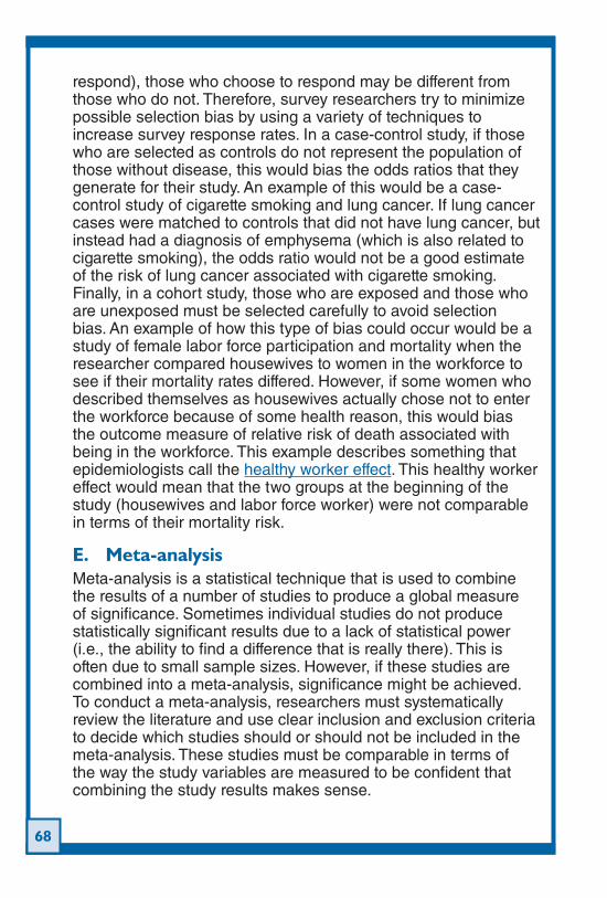
68
respond), those who choose to respond may be different from those who do not. Therefore, survey researchers try to minimize possible selection bias by using a variety of techniques to increase survey response rates. In a case-control study, if those who are selected as controls do not represent the population of those without disease, this would bias the odds ratios that they generate for their study. An example of this would be a case-control study of cigarette smoking and lung cancer. If lung cancer cases were matched to controls that did not have lung cancer, but instead had a diagnosis of emphysema (which is also related to cigarette smoking), the odds ratio would not be a good estimate of the risk of lung cancer associated with cigarette smoking. Finally, in a cohort study, those who are exposed and those who are unexposed must be selected carefully to avoid selection bias. An example of how this type of bias could occur would be a study of female labor force participation and mortality when the researcher compared housewives to women in the workforce to see if their mortality rates differed. However, if some women who described themselves as housewives actually chose not to enter the workforce because of some health reason, this would bias the outcome measure of relative risk of death associated with being in the workforce. This example describes something that epidemiologists call the healthy worker effect. This healthy worker effect would mean that the two groups at the beginning of the study (housewives and labor force worker) were not comparable in terms of their mortality risk.
E. Meta-analysisMeta-analysis is a statistical technique that is used to combine the results of a number of studies to produce a global measure of significance. Sometimes individual studies do not produce statistically significant results due to a lack of statistical power (i.e., the ability to find a difference that is really there). This is often due to small sample sizes. However, if these studies are combined into a meta-analysis, significance might be achieved. To conduct a meta-analysis, researchers must systematically review the literature and use clear inclusion and exclusion criteria to decide which studies should or should not be included in the meta-analysis. These studies must be comparable in terms of the way the study variables are measured to be confident that combining the study results makes sense.
69
One of the more common ways to display the results of a meta-analysis is through a graph called a forest plot. A description of the parts of the forest plot is provided in the legend of Figure 12 that appeared in an article by Straetemans and colleagues in 2011.
(I-squared = 88.6%, p = 0.000). The Study ID on the Y-axis includes the name of the first author and publication year; for each study the central square indicates the mortality percentage and the horizontal line denotes the 95% confidence interval (CI) around the mortality percentage. The size of the square indicates the impact the specific study has on the point estimate of the pooled estimate. The vertical dashed line indicates the pooled mortality percentage and the outer edges of the diamond represent the 95% confidence interval (CI) around the pooled estimate; the X-axis indicates the scale of mortality percentage. doi:10.1371/journal.pone.0020755.g004
Figure 12. Forest plotSource: Straetemans M, Glaziou P, Bierrenbach AL, Sismanidis C, van der Werf MJ (2011) Assessing Tuberculosis Case Fatality Ratio: A Meta-Analysis. PLoS ONE 6(6): e20755. doi:10.1371/journal.pone.0020755. Reprinted here with permission.
This forest plot shows there was some variability in the mortality estimates produced by each of these studies. Some estimate were very low (e.g., Ackah 95 and Ciglenecki 07a) and some were high (e.g., Kelly 99). Also the confidence intervals around these estimates were sometimes very narrow (e.g., Cayla 09) and sometimes very wide (e.g., Kelly 99). When all the data were combined using meta-analysis statistical software, the pooled estimate is a 5% overall mortality rate among HIV uninfected TB patients.
70
Molecular Epidemiology: Genotyping and TB 9. Control(Text for this section was based on material provided by the Centers for Disease Control and Prevention.)
A. What Is TB Genotyping?Our understanding of TB epidemiology and transmission, which was traditionally based on findings of case and contact tracing, has been enhanced in recent years by TB genotyping. TB genotyping is a laboratory-based genetic analysis of the bacteria that cause TB disease (i.e., any of the organisms in the Mycobacterium tuberculosis complex) that can identify the strain of M. tuberculosis present in an isolate (positive TB culture) from a person with TB disease.
When TB bacteria reproduce, they create new genetically identical bacilli. However, in some cases, random mutations occur spontaneously, creating different strains of TB, which then reproduce. Because of this, there are now many strains of M. tuberculosis present around the world. Cases with matching genotypes are probably connected to each other somehow, although the connections might not be recent or obvious. For example, two persons whose TB strains match by genotype may not know one another, but they may both have been exposed to the same infectious case at a social club that they both go to.
Using TB genotyping to identify the strain of M. tuberculosis can assist in:
Confirming if epidemiologically linked patients are actually •connected by transmission, or if they could have acquired TB from different sourcesIdentifying patients that may be connected to other cases •by recent transmission, but were not found through contact investigationTracing the chain of TB transmission•Detecting and controlling outbreaks* earlier•Identifying false-positive TB culture results more easily•Identifying unknown relationships between cases and •unrecognized places of transmission
71
Detecting transmission between patients in different •jurisdictionsEvaluating effectiveness of routine contact investigations.•
* Remember: A true outbreak of TB generally requires that there be both more cases than expected within a geographic area or population during a particular time period, and evidence of recent transmission of M. tuberculosis among those cases.
TB programs may take a variety of steps after analyzing TB genotyping results including: conducting or expanding outbreak investigations, performing cluster investigations to locate epidemiologic links between patients, or assessing if a specific patient had a false-positive culture result. Further, since national and international databases and collections of clinical M. tuberculosis strains have been established in different areas worldwide, using these databases to compare strains isolated from individual TB patients might increase understanding of TB transmission pathways.
B. National TB Genotyping Service and the TB Genotyping Information Management SystemSince 2004, CDC has funded the National TB Genotyping Service (NTGS) to provide genotyping to TB programs in the United States and its territories. There are two genotyping techniques routinely used by the NTGS. These are1. Spoligotyping, also known as spacer oligonucleotide
genotyping2. MIRU, also known as mycobacterial interspersed repetitive
unit analysis – variable number tandem repeat analysis (MIRU-VNTR)
Spoligotype results are shown as 15 characters (e.g., 000000000003771). All isolates genotyped by MIRU analysis since April 2009 are reported with 24 characters: 12 characters (MIRU) followed by an additional 12 characters (MIRU2), which together are referred to as 24-locus MIRU-VNTR. Only the first 12-character MIRU was routinely performed on isolates before April 2009. The spoligotype and MIRU results are combined by the NTGS into a shorthand label, known as a PCRType (e.g., PCR00041). In 2011, CDC introduced a new label system that includes spoligotype and 24-locus MIRU-VNTR. Each unique combination of spoligotype and 24-locus MRU-VNTR will be assigned a GENType (e.g., G01974).
72
Both GENType and PCRType are nation-wide designations, meaning the same GENType will be assigned no matter which state the genotype is seen in. The NTGS reports genotyping results to the submitting TB programs and laboratories and CDC’s Division of TB Elimination (DTBE). Genotyping information on specific TB cases is available to state health departments through the TB Genotyping Information Management System (TB GIMS), the secured online national database of TB genotyping and case information. Local health departments obtain access to genotyping data in various ways, usually either through TB GIMS directly or from the state TB program.
TB GIMS cluster alerts are an important part of genotyping surveillance. Cluster alerts are an automatic function within TB GIMS that notifies users when there are unusual geographic concentrations of specific genotype clusters in their jurisdiction compared to the rest of the country. However, not all genotype clusters or TB GIMS cluster alerts represent outbreaks. When genotype clusters are found, additional investigation is needed.
For more information about TB GIMS, please refer to the CDC website on TB GIMS: http://www.cdc.gov/tb/publications/factsheets/statistics/gims.htm
C. Using TB Genotyping in TB Outbreak DetectionIn order to detect TB outbreaks, it is important for public health programs to follow up reports of concern from providers or the public and to monitor for:
Contact investigation findings that suggest a TB outbreak •might be happeningUnexpected increases in TB case numbers or TB case rates •within their jurisdictionsChanges in the occurrence and distribution of TB cases, •according to cases’ demographics, TB risk factors, TB drug resistance patterns, and genotypesGenotype clusters, new or uncommon TB genotypes, and •unexpected increases in TB genotypes common seen in their jurisdictions
73
D. Cluster InvestigationsCluster investigations can help public health investigators find or confirm connections (i.e., relationships or associations) among cases with matching genotypes. These connections are referred to as epidemiologic links, or epi links. When “known exposures, affiliations or connections” to other cases or epi links1 are found among clustered cases, it suggests there might have been recent transmission among them.Source of epi link definition: http://emergency.cdc.gov/urdo/pdf/LineListTemplate.pdf
The main objective of a cluster investigation is to determine whether it is likely there was recent transmission among cases in a genotype cluster. Even when cases within a genotype cluster have epi links to one another, it does not always mean transmission was recent, or that transmission is continuing. For example, a cluster of cases could happen after an influx of refugees from a region where TB is endemic.
Cluster investigations generally have two stages. The first stage involves reviewing information already on hand about the clustered cases. This stage might include:
Reviewing information in TB GIMS, and local or state •databasesDiscussing cases with program staff that are familiar with •themSystematically reviewing patient records•
Programs can often determine whether a cluster could be an outbreak based on this easily accessible information. In some situations, additional (new) information will be needed.
During the second stage of investigation new information can be obtained from re-interviewing cases and making site visits to locations where transmission might have happened.
Epidemiologic links that are found through cluster investigations can be used to help identify where transmission could have happened and establish if it was recent. For example, if five cases from different neighborhoods, workplaces, and age groups have matching genotypes, a cluster investigation might find that
74
over the previous 6 months, every one of the cases had gone to the same sports bar to watch football. The cases might not have considered the sports bar an important location to mention during their contact investigation interviews, or they might not have known each other by name. In this example, a cluster investigation could help find an important epi link among the cases (the sports bar). This may be useful in identifying additional contacts who may have been exposed to TB.
Finding or confirming connections (epi links) among cases in a suspected outbreak can be difficult when genotyping information is not available. Some situations where genotyping information might not be available include:
Clinical cases (no culture available)•Culture-negative cases•Cases whose culture results are still pending•
In such situations, if an unexpected increase in cases and epidemiologic links among the cases can be reasonably established, it is usually advisable for public health programs to proceed as though there is an outbreak.
75
Part Three: Putting It All Together
TB Case Study10. This section creates a scenario in which you are a TB control officer and it will allow you to use some of the concepts introduced in the Basic Epidemiology for Tuberculosis Program Staff manual. Start by reading the background information below and then work through the remainder of the exercise. You will need to use a calculator for a few simple calculations. This exercise will provide you with an opportunity to combine what you already know about TB control to the interpretation of the epidemiologic data provided.
A. How to Use TB Surveillance Data in TB ControlOriginally prepared by the CDC for the TB Program Managers’ Course, Modified for NJMS Global TB Institute 2012
Background InformationYou were recently appointed TB control officer for State X. After a few days on the job, you begin to notice a trend that has emerged over the past several years. Historically, the annual TB incidence rate for State X has been less than the national average. From 2001 through 2006 the rate was less than 3.5 cases per 100,000 population, which would have put State X in the low-incidence category. However, the case count began increasing in 2002 at an average rate of 9% per year, and, by 2007, the incidence rate has increased to 4.2 cases per 100,000. As the new TB control officer, you will need to determine what factors are contributing to the rise in TB incidence in your state.
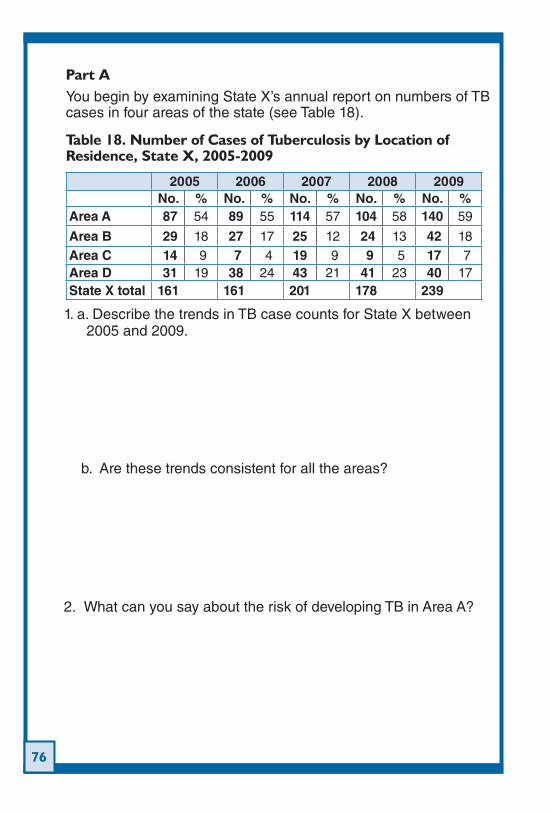
76
Part AYou begin by examining State X’s annual report on numbers of TB cases in four areas of the state (see Table 18).
Table 18. Number of Cases of Tuberculosis by Location of Residence, State X, 2005-2009
2005 2006 2007 2008 2009No. % No. % No. % No. % No. %
Area A 87 54 89 55 114 57 104 58 140 59
Area B 29 18 27 17 25 12 24 13 42 18Area C 14 9 7 4 19 9 9 5 17 7Area D 31 19 38 24 43 21 41 23 40 17State X total 161 161 201 178 239
1. a. Describe the trends in TB case counts for State X between 2005 and 2009.
b. Are these trends consistent for all the areas?
2. What can you say about the risk of developing TB in Area A?
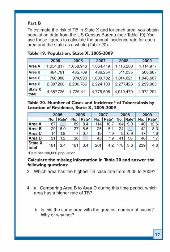
77
Part BTo estimate the risk of TB in State X and for each area, you obtain population data from the US Census Bureau (see Table 19). You use these figures to calculate the annual incidence rate for each area and the state as a whole (Table 20).
Table 19. Population, State X, 2005-2009
2005 2006 2007 2008 2009Area A 1,054,817 1,058,943 1,064,419 1,116,200 1,114,977Area B 484,761 485,709 486,254 511,035 508,667Area C 760,880 974,993 1,000,702 1,014,821 1,048,667Area D 2,387,268 2,206,766 2,224,133 2,277,423 2,299,983State X total 4,687,726 4,726,411 4,775,508 4,919,479 4,972,294
Table 20. Number of Cases and Incidence* of Tuberculosis by Location of Residence, State X, 2005-2009
2005 2006 2007 2008 2009No. Rate* No. Rate* No. Rate* No. Rate* No. Rate*
Area A 87 89 8.4 114 10.7 104 9.3 140 12.6Area B 29 6.0 27 5.6 25 5.1 24 42 8.3Area C 14 1.8 7 0.7 19 1.9 9 0.9 17 1.6Area D 31 1.3 38 43 1.9 41 1.8 40 1.7State X total 161 3.4 161 3.4 201 4.2 178 3.6 239 4.8
*Rate per 100,000 population.
Calculate the missing information in Table 20 and answer the following questions:3. Which area has the highest TB case rate from 2005 to 2009?
4. a. Comparing Area B to Area D during this time period, which area has a higher rate of TB?
b. Is this the same area with the greatest number of cases? Why or why not?
78
Part CYou inform the state epidemiologist of the results of your analysis. He too is concerned about the increasing case numbers and case rates in your state. He advises you to create a detailed report on the TB situation in the state, explaining the increasing TB trend. He also wants your recommendations for future priorities in TB prevention and control.
To draft your report and recommendations for the state epidemiologist you obtain data on TB cases for the past 9 years in State X (see Table 21). You also obtain detailed population estimates for various groups in the state from the US Census Bureau (see Table 22*).
*Foreign-born population extrapolated from 2000 US census.
Calculate the missing information in Table 23 and answer the following questions:5. What is the overall trend in TB incidence for State X from 2001
to 2009?
6. Who is at highest risk of TB in State X?
7. Does risk (as estimated by rate) measure the problem?
8. What are some explanations for the increasing rate of disease seen in State X?
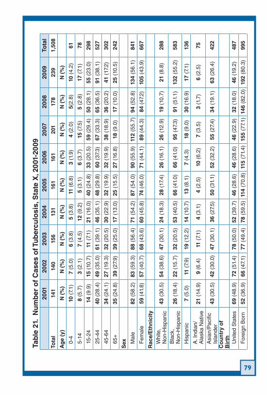
79
Tab
le 2
1. N
um
ber
of
Cas
es o
f Tu
ber
culo
sis,
Sta
te X
, 20
01-2
009
2001
2002
2003
2004
2005
2006
2007
2008
2009
Tota
l
Tota
l14
114
015
613
116
116
120
117
823
91,
508
Ag
e (y
)N
(%
)N
(%
)N
(%
)N
(%
)N
(%
)N
(%
)N
(%
)N
(%
)N
(%
)
0-
4 10
(7.
1)7
(5.0
)6
(3.8
)5
(3.8
)11
(6.
8)3
(1.9
)4
(2.0
)5(
2.8)
10 (
4.2)
61
5-
14
8 (5
.7)
3 (2
.1)
7 (4
.5)
12 (
9.2)
5 (3
.1)
6 (3
.7)
15 (
7.5)
5 (2
.8)
17 (
7.1)
78
15
-24
14 (
9.9)
15 (
10.7
)11
(7.
1)21
(16
.0)
40 (
24.8
)33
(20
.5)
59 (
29.4
)50
(28
.1)
55 (
23.0
)29
8
25
-44
40 (
28.4
)49
(35
.0)
61 (
39.1
)46
(35
.1)
48 (
29.8
)60
(37
.3)
67 (
33.3
)65
(36
.5)
91 (
38.1
)52
7
45
-64
34 (
24.1
)27
(19
.3)
32 (
20.5
)30
(22
.9)
32 (
19.9
)32
(19
.9)
38 (
18.9
)36
(20
.2)
41 (
17.2
)30
2
65
+35
(24
.8)
39 (
27.9
)39
(25
.0)
17 (
13.0
)25
(15
.5)
27 (
16.8
)18
(9.
0)17
(10
.0)
25 (
10.5
)24
2
Sex
M
ale
82 (
58.2
)83
(59
.3)
88 (
56.4
)71
(54
.2)
87 (
54.0
)90
(55
.9)
112
(55.
7)94
(52
.8)
134
(56.
1)84
1
F
emal
e59
(41
.8)
57 (
40.7
)68
(43
.6)
60 (
45.8
)74
(46
.0)
71 (
44.1
)89
(44
.3)
84 (
47.2
)10
5 (4
3.9)
667
Rac
e/E
thn
icit
y
Whi
te,
N
on-H
ispa
nic
43 (
30.5
)54
(38
.6)
47 (
30.1
)24
(18
.3)
28 (
17.4
)26
(16
.1)
26 (
12.9
)19
(10
.7)
21 (
8.8)
288
B
lack
,
Non
-His
pani
c26
(18
.4)
22 (
15.7
)32
(20
.5)
53 (
40.5
)66
(41
.0)
66 (
41.0
)95
(47
.3)
91 (
51.1
)13
2 (5
5.2)
583
H
ispa
nic
7 (5
.0)
11 (
7.9)
19 (
12.2
)14
(10
.7)
13 (
8.1)
7 (4
.3)
18 (
9.0)
30 (
16.9
)17
(7.
1)13
6
A
. Ind
ian/
Ala
ska
Nat
ive
21 (
14.9
)9
(6.4
)11
(7.
1)4
(3.1
)4
(2.5
)10
(6.
2)7
(3.5
)3
(1.7
)6
(2.5
)75
A
sian
/Pac
ific
Isla
nder
43 (
30.5
)42
(30
.0)
47 (
30.1
)36
(27
.5)
50 (
31.1
)52
(32
.2)
55 (
27.4
)34
(19
.1)
63 (
26.4
)42
2
Co
un
try
of
Bir
th
Uni
ted
Sta
tes
69 (
48.9
)72
(51
.4)
78 (
50.0
)52
(39
.7)
46 (
28.6
)46
(28
.6)
46 (
22.9
)32
(18
.0)
46 (
19.2
)48
7
F
orei
gn B
orn
52 (
36.9
)66
(47
.1)
77 (
49.4
)78
(59
.5)
114
(70.
8)11
5 (7
1.4)
155
(77.
1)14
6 (8
2.0)
192
(80.
3)99
5
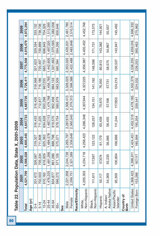
80
Tab
le 2
2. P
op
ula
tio
n D
ata,
Sta
te X
, 20
01-2
009
2001
2002
2003
2004
2005
2006
2007
2008
2009
Tota
l4,
521,
709
4,56
6,02
84,
605,
445
4,64
7,72
34,
687,
726
4,72
6,41
14,
775,
508
4,91
9,47
94,
972,
294
Ag
e (y
r)
0-4
331,
672
326,
087
319,
327
316,
433
316,
426
318,
568
321,
623
329,
594
333,
132
5-
1470
2,50
370
9,33
471
1,80
871
1,22
571
2,81
771
6,18
672
0,49
773
0,88
973
8,73
6
15-2
461
0,16
061
6,92
962
5,36
363
4,62
865
0,29
866
7,25
568
3,73
169
6,84
570
4,32
6
25-4
41,
476,
225
1,48
1,26
61,
484,
578
1,48
7,11
31,
474,
748
1,45
6,76
01,
442,
600
1,49
7,32
01,
513,
395
45
-64
834,
877
861,
286
888,
798
919,
570
952,
458
984,
133
1,02
1,66
31,
070,
565
1,08
2,05
8
65+
566,
272
571,
126
575,
571
578,
754
580,
979
583,
509
585,
394
594,
266
600,
646
Sex
M
ale
2,22
1,95
82,
244,
739
2,26
5,79
72,
287,
678
2,30
8,41
32,
328,
025
2,35
3,02
02,
435,
631
2,46
1,78
0
Fem
ale
2,29
9,75
12,
321,
289
2,33
9,64
82,
360,
045
2,37
9,31
32,
398,
386
2,42
2,48
82,
483,
848
2,51
0,51
4
Rac
e/E
thn
icit
y
W
hite
,
Non
-His
pani
c4,
205,
303
4,23
4,71
84,
258,
422
4,28
6,34
84,
307,
944
4,32
7,22
54,
356,
987
4,40
5,45
24,
452,
748
B
lack
,
Non
-His
pani
c11
1,61
111
7,59
712
3,12
212
8,25
713
4,15
114
1,19
214
8,59
617
1,73
117
3,57
5
H
ispa
nic
55,1
1757
,674
61,1
7965
,439
70,6
7076
,050
80,8
1314
3,38
214
4,92
1
A
. Ind
ian/
Ala
ska
Nat
ive
54,3
6955
,235
56,0
6656
,435
57,1
0857
,731
58,5
7554
,967
55,5
57
A
sian
/Pac
ific
Is
land
er95
,309
100,
804
106,
666
111,
244
117,
853
124,
213
130,
537
143,
947
145,
492
Co
un
try
of
Bir
th
U
nite
d S
tate
s4,
368,
423
4,39
8,91
14,
424,
451
4,45
2,51
94,
478,
185
4,50
2,37
94,
536,
255
4,65
9,01
64,
696,
332
F
orei
gn B
orn
153,
286
167,
117
180,
994
195,
204
209,
541
224,
032
239,
253
260,
463
275,
962
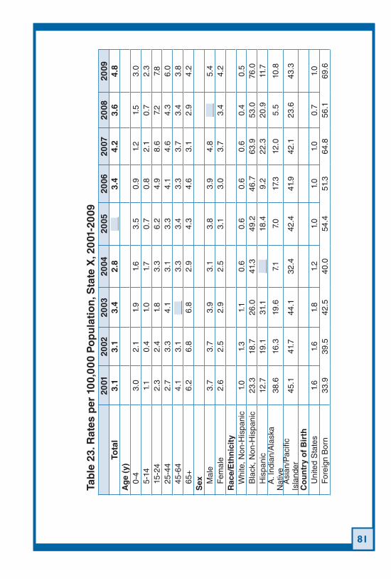
81
Tab
le 2
3. R
ates
per
10
0,0
00
Po
pu
lati
on
, Sta
te X
, 20
01-2
009
2001
2002
2003
2004
2005
2006
2007
2008
2009
Tota
l3.
13.
13.
42.
8__
_3.
44.
23.
64.
8A
ge
(y)
0-
43.
02.
11.
91.
63.
50.
91.
21.
53.
0
5-14
1.1
0.4
1.0
1.7
0.7
0.8
2.1
0.7
2.3
15
-24
2.3
2.4
1.8
3.3
6.2
4.9
8.6
7.2
7.8
25
-44
2.7
3.3
4.1
3.1
3.3
4.1
4.6
4.3
6.0
45
-64
4.1
3.1
___
3.3
3.4
3.3
3.7
3.4
3.8
65
+6.
26.
86.
82.
94.
34.
63.
12.
94.
2S
ex
Mal
e3.
73.
73.
93.
13.
83.
94.
8__
_5.
4
Fem
ale
2.6
2.5
2.9
2.5
3.1
3.0
3.7
3.4
4.2
Rac
e/E
thn
icit
y
Whi
te, N
on-H
ispa
nic
1.0
1.3
1.1
0.6
0.6
0.6
0.6
0.4
0.5
B
lack
, Non
-His
pani
c23
.318
.726
.041
.349
.246
.763
.953
.076
.0
His
pani
c12
.719
.131
.1__
_18
.49.
222
.320
.911
.7
A. I
ndia
n/A
lask
a N
ativ
e38
.616
.319
.67.
17.
017
.312
.05.
510
.8
Asi
an/P
acifi
c Is
land
er45
.141
.744
.132
.442
.441
.942
.123
.643
.3
Co
un
try
of
Bir
th
Uni
ted
Sta
tes
1.6
1.6
1.8
1.2
1.0
1.0
1.0
0.7
1.0
F
orei
gn B
orn
33.9
39.5
42.5
40.0
54.4
51.3
64.8
56.1
69.6
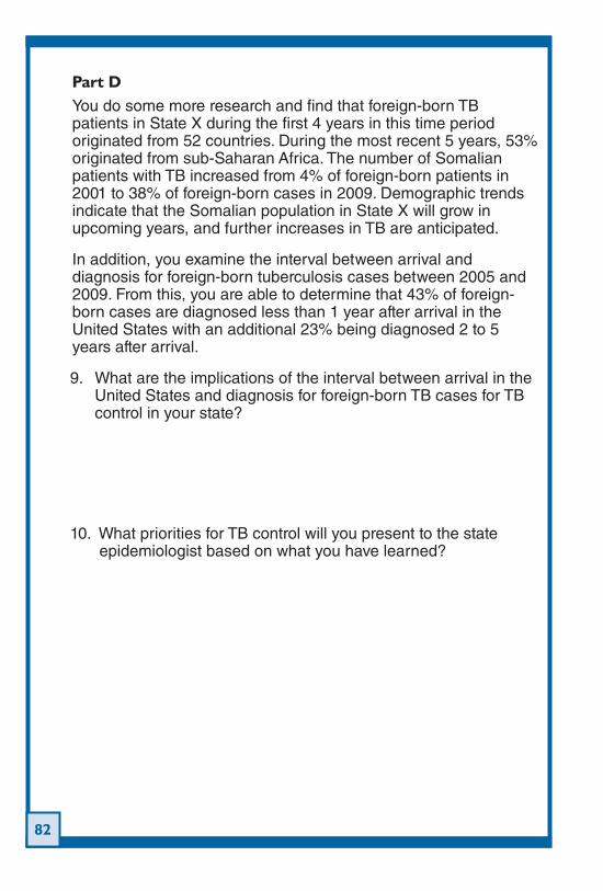
82
Part DYou do some more research and find that foreign-born TB patients in State X during the first 4 years in this time period originated from 52 countries. During the most recent 5 years, 53% originated from sub-Saharan Africa. The number of Somalian patients with TB increased from 4% of foreign-born patients in 2001 to 38% of foreign-born cases in 2009. Demographic trends indicate that the Somalian population in State X will grow in upcoming years, and further increases in TB are anticipated.
In addition, you examine the interval between arrival and diagnosis for foreign-born tuberculosis cases between 2005 and 2009. From this, you are able to determine that 43% of foreign-born cases are diagnosed less than 1 year after arrival in the United States with an additional 23% being diagnosed 2 to 5 years after arrival.
9. What are the implications of the interval between arrival in the United States and diagnosis for foreign-born TB cases for TB control in your state?
10. What priorities for TB control will you present to the state epidemiologist based on what you have learned?
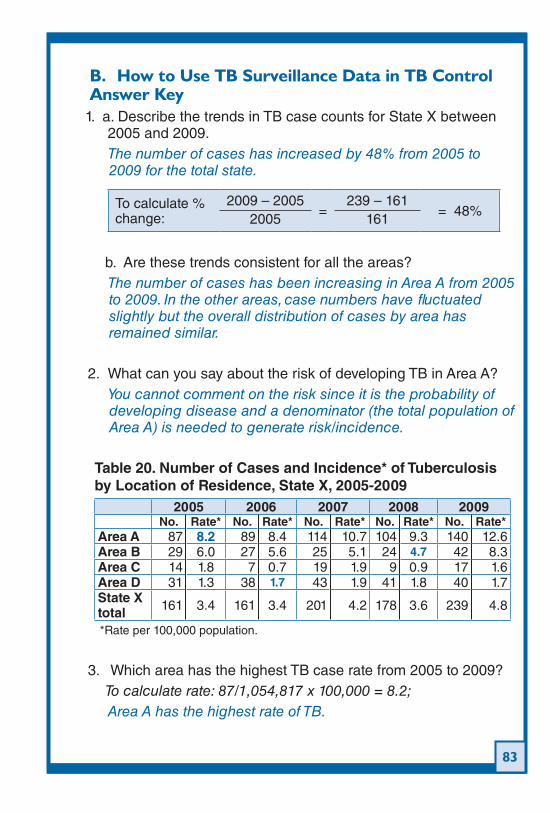
83
B. How to Use TB Surveillance Data in TB Control Answer Key
1. a. Describe the trends in TB case counts for State X between 2005 and 2009.The number of cases has increased by 48% from 2005 to 2009 for the total state.
To calculate % change:
2009 – 2005=
239 – 161= 48%
2005 161
b. Are these trends consistent for all the areas?The number of cases has been increasing in Area A from 2005 to 2009. In the other areas, case numbers have fluctuated slightly but the overall distribution of cases by area has remained similar.
2. What can you say about the risk of developing TB in Area A?You cannot comment on the risk since it is the probability of developing disease and a denominator (the total population of Area A) is needed to generate risk/incidence.
Table 20. Number of Cases and Incidence* of Tuberculosis by Location of Residence, State X, 2005-2009
2005 2006 2007 2008 2009No. Rate* No. Rate* No. Rate* No. Rate* No. Rate*
Area A 87 8.2 89 8.4 114 10.7 104 9.3 140 12.6Area B 29 6.0 27 5.6 25 5.1 24 4.7 42 8.3Area C 14 1.8 7 0.7 19 1.9 9 0.9 17 1.6Area D 31 1.3 38 1.7 43 1.9 41 1.8 40 1.7State X total 161 3.4 161 3.4 201 4.2 178 3.6 239 4.8
*Rate per 100,000 population.
3. Which area has the highest TB case rate from 2005 to 2009?To calculate rate: 87/1,054,817 x 100,000 = 8.2;Area A has the highest rate of TB.
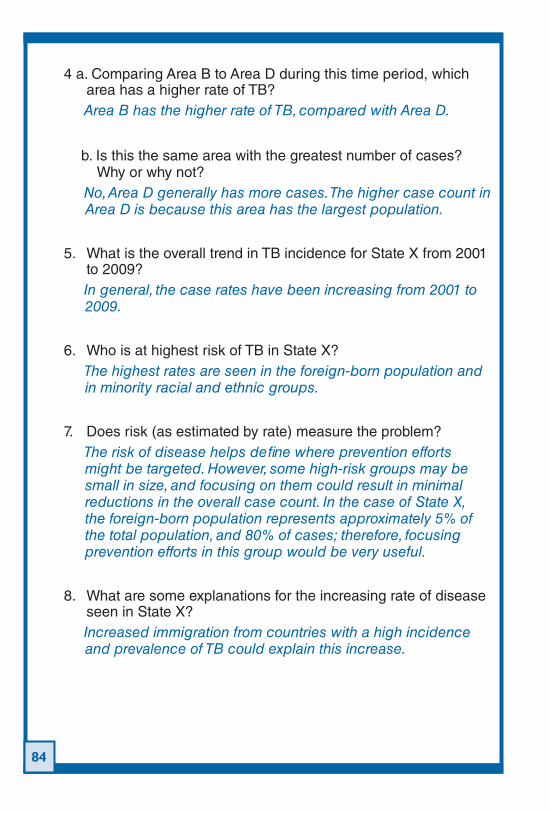
84
4 a. Comparing Area B to Area D during this time period, which area has a higher rate of TB?Area B has the higher rate of TB, compared with Area D.
b. Is this the same area with the greatest number of cases? Why or why not?No, Area D generally has more cases. The higher case count in Area D is because this area has the largest population.
5. What is the overall trend in TB incidence for State X from 2001 to 2009?In general, the case rates have been increasing from 2001 to 2009.
6. Who is at highest risk of TB in State X?The highest rates are seen in the foreign-born population and in minority racial and ethnic groups.
7. Does risk (as estimated by rate) measure the problem?The risk of disease helps define where prevention efforts might be targeted. However, some high-risk groups may be small in size, and focusing on them could result in minimal reductions in the overall case count. In the case of State X, the foreign-born population represents approximately 5% of the total population, and 80% of cases; therefore, focusing prevention efforts in this group would be very useful.
8. What are some explanations for the increasing rate of disease seen in State X?Increased immigration from countries with a high incidence and prevalence of TB could explain this increase.
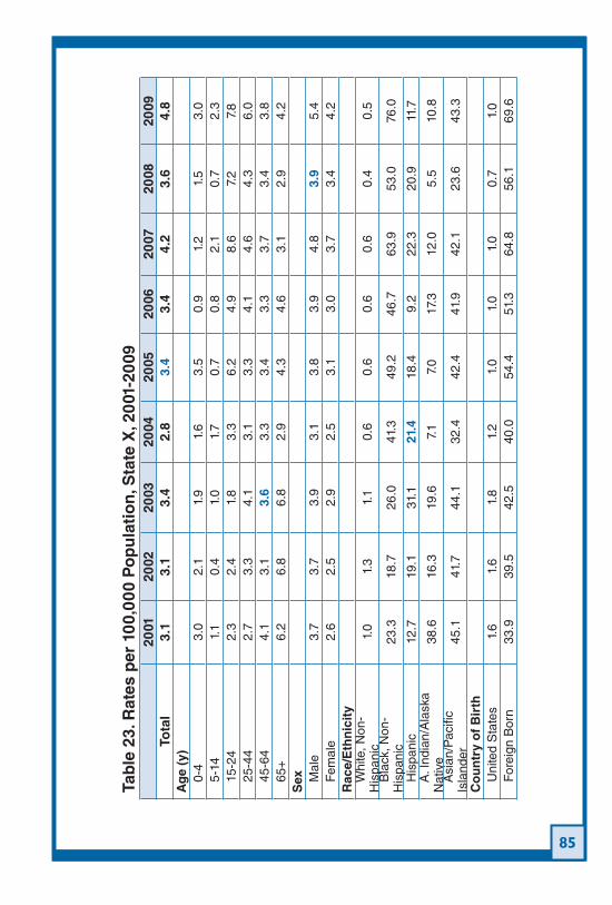
85
Tab
le 2
3. R
ates
per
10
0,0
00
Po
pu
lati
on
, Sta
te X
, 20
01-2
009
2001
2002
2003
2004
2005
2006
2007
2008
2009
Tota
l3.
13.
13.
42.
83.
43.
44.
23.
64.
8A
ge
(y)
0-
43.
02.
11.
91.
63.
50.
91.
21.
53.
0
5-14
1.1
0.4
1.0
1.7
0.7
0.8
2.1
0.7
2.3
15
-24
2.3
2.4
1.8
3.3
6.2
4.9
8.6
7.2
7.8
25
-44
2.7
3.3
4.1
3.1
3.3
4.1
4.6
4.3
6.0
45
-64
4.1
3.1
3.6
3.3
3.4
3.3
3.7
3.4
3.8
65
+6.
26.
86.
82.
94.
34.
63.
12.
94.
2S
ex
Mal
e3.
73.
73.
93.
13.
83.
94.
83.
95.
4
Fem
ale
2.6
2.5
2.9
2.5
3.1
3.0
3.7
3.4
4.2
Rac
e/E
thn
icit
y
Whi
te, N
on-
His
pani
c1.
01.
31.
10.
60.
60.
60.
60.
40.
5
Bla
ck, N
on-
His
pani
c23
.318
.726
.041
.349
.246
.763
.953
.076
.0
H
ispa
nic
12.7
19.1
31.1
21.4
18.4
9.2
22.3
20.9
11.7
A
. Ind
ian/
Ala
ska
Nat
ive
38.6
16.3
19.6
7.1
7.0
17.3
12.0
5.5
10.8
A
sian
/Pac
ific
Isla
nder
45.1
41.7
44.1
32.4
42.4
41.9
42.1
23.6
43.3
Co
un
try
of
Bir
th
Uni
ted
Sta
tes
1.6
1.6
1.8
1.2
1.0
1.0
1.0
0.7
1.0
F
orei
gn B
orn
33.9
39.5
42.5
40.0
54.4
51.3
64.8
56.1
69.6
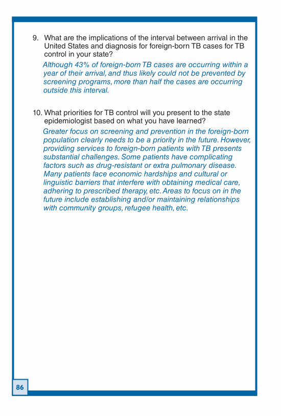
86
9. What are the implications of the interval between arrival in the United States and diagnosis for foreign-born TB cases for TB control in your state?Although 43% of foreign-born TB cases are occurring within a year of their arrival, and thus likely could not be prevented by screening programs, more than half the cases are occurring outside this interval.
10. What priorities for TB control will you present to the state epidemiologist based on what you have learned?Greater focus on screening and prevention in the foreign-born population clearly needs to be a priority in the future. However, providing services to foreign-born patients with TB presents substantial challenges. Some patients have complicating factors such as drug-resistant or extra pulmonary disease. Many patients face economic hardships and cultural or linguistic barriers that interfere with obtaining medical care, adhering to prescribed therapy, etc. Areas to focus on in the future include establishing and/or maintaining relationships with community groups, refugee health, etc.
87
Appendix I – Glossary of Epidemiology TermsGlossary terms taken from Principles of Epidemiology in Public Health Practice, 3rd Edition. Developed by: U.S. Department of Health and Human Services, Centers for Disease Control and Prevention, Office of Workforce and Career Development, Career Development Division, Atlanta, GA 30333. Technical content by: Richard C. Dicker, MD, MSc, Lead Author, Fatima Coronado, MD, MPH, Denise Koo, MD, MPH, Roy Gibson Parrish, II, MD. Published by the Public Health Foundation in November, 2006. Retrieved from: http://www.cdc.gov/excite/library/glossary.htm
agent a factor (e.g., a microorganism or chemical substance) or form of energy whose presence, excessive presence, or in the case of deficiency diseases, relative absence is essential for the occurrence of a disease or other adverse health outcome.
association the statistical relation between two or more events, characteristics, or other variables.
attribute a risk factor that is an intrinsic characteristic of the individual person, animal, plant, or other type of organism under study (e.g., genetic susceptibility, age, sex, breed, weight).
axis one of the dimensions of a graph. In a rectangular graph, the x-axis is the horizontal axis and the y-axis is the vertical axis.
bar chart a visual display in which each category of a variable is represented by a bar or column; bar charts are used to illustrate variations in size among categories.
bias a systematic deviation of results or inferences from the truth or processes leading to such systematic deviation; any systematic tendency in the collection, analysis, interpretation, publication, or review of data that can lead to conclusions that are systematically different from the truth. In epidemiology, bias does not imply intentional deviation.
bias, information systematic difference in the collection of data regarding the participants in a study (e.g., about exposures in a case-control study, or about health outcomes in a cohort study) that leads to an incorrect result (e.g., risk ratio or odds ratio) or inference.
88
bias, selection systematic difference in the enrollment of participants in a study that leads to an incorrect result (e.g., risk ratio or odds ratio) or inference.
case an instance of a particular disease, injury, or other health conditions that meets selected criteria (see also case definition). Using the term to describe the person rather than the health condition is discouraged (see also case-patient).
case definition a set of uniformly applied criteria for determining whether a person should be identified as having a particular disease, injury, or other health condition. In epidemiology, particularly for an outbreak investigation, a case definition specifies clinical criteria and details of time, place, and person.
case-fatality rate (also called case-fatality ratio) the proportion of persons with a particular condition (e.g., patients) who die from that condition. The denominator is the number of persons with the condition; the numerator is the number of cause-specific deaths among those persons.
case, index the first case or instance of a patient coming to the attention of health authorities.
case-patient in a case-control study, a person who has the disease, injury, or other health condition that meets the case definition (see also case).
cause of disease a factor (e.g., characteristic, behavior, or event) that directly influences the occurrence of a disease. Reducing such a factor among a population should reduce occurrence of the disease.
census the enumeration of an entire population, usually including details on residence, age, sex, occupation, racial/ethnic group, marital status, birth history, and relationship to the head of the household.
central location (also called central tendency) a statistical measurement to quantify the middle or the center of a distribution. Of the multiple ways to define central tendency, the most common ways are the mean, median, and mode.
89
class a grouping of observations of values of a variable. Classes are created for convenience in analyzing frequency. (see also class interval).
class interval the span of values of a continuous variable that are grouped into a single category (see also class), usually to create a frequency distribution for that variable.
class limits the values at the upper and lower ends of a class interval.
cluster an aggregation of cases of a disease, injury, or other health condition (particularly cancer and birth defects) in a circumscribed area during a particular period without regard to whether the number of cases is more than expected (often the expected number is not known).
cohort a well-defined group of persons who have had a common experience or exposure and are then followed up, as in a cohort study or prospective study, to determine the incidence of new diseases or health events.
comparison group a group in an analytic study (e.g., a cohort or case-control study) with whom the primary group of interest (exposed group in a cohort study or case-patients in a case-control study) is compared. The comparison group provides an estimate of the background or expected incidence of disease (in a cohort study) or exposure (in a case-control study).
confidence interval a range of values for a measure (e.g., rate or odds ratio) constructed so that the range has a specified probability (often, but not necessarily, 95%) of including the true value of the measure.
confidence limits the end points (i.e., the minimum and maximum values) of a confidence.
confounding the distortion of the association between an exposure and a health outcome by a third variable that is related to both.
contact exposure to a source of an infection; a person who has been exposed.
90
control in a case-control study, a member of the group of persons without the health problem under study (see also comparison group and study, case-control).
crude when referring to a rate, an overall or summary rate for a population, without adjustment.
demographic information personal characteristics of a person or group (e.g., age, sex, race/ethnicity, residence, and occupation) demographic information is used in descriptive epidemiology to characterize patients or populations.
denominator the lower portion of a fraction; used in calculating a ratio, proportion, or rate. For a rate, the denominator is usually the mid-interval population.
determinant any factor that brings about change in a health condition or in other defined characteristics (see also cause and risk factor).
distribution in epidemiology, the frequency and pattern of health-related characteristics and events in a population; in statistics, the frequency and pattern of the values or categories of a variable.
endemic the constant presence of an agent or health condition within a given geographic area or population; can also refer to the usual prevalence of an agent or condition.
environmental factor an extrinsic factor (e.g., geology, climate, insects, sanitation, or health services) that affects an agent and the opportunity for exposure.
epidemic the occurrence of more cases of disease, injury, or other health condition than expected in a given area or among a specific group of persons during a particular period. Usually, the cases are presumed to have a common cause or to be related to one another in some way (see also outbreak).
epidemiology the study of the distribution and determinants of health conditions or events among populations and the application of that study to control health problems.
epidemiology, analytic the aspect of epidemiology concerned with why and how a health problem occurs. Analytic epidemiology
91
uses comparison groups to provide baseline or expected values so that associations between exposures and outcomes can be quantified and hypotheses about the cause of the problem can be tested (see also study, analytic).
epidemiology, descriptive the aspect of epidemiology concerned with organizing and summarizing data regarding the persons affected (e.g., the characteristics of those who became ill), time (e.g., when they become ill), and place (e.g., where they might have been exposed to the cause of illness).
exposed group a group whose members have had contact with a suspected cause of, or possess a characteristic that is a suspected determinant of, a particular health problem.
exposure having come into contact with a cause of, or possessing a characteristic that is a determinant of, a particular health problem.
false-negative a negative test result for a person who actually has the condition; similarly, a person who has the disease (perhaps mild or variant) but who does not fit the case definition, or a patient or outbreak not detected by a surveillance system.
false-positive a positive test result for a person who actually does not have the condition. Similarly, a person who does not have the disease but who nonetheless fits the case definition, or a patient or outbreak erroneously identified by a surveillance system.
forest plot a graph that displays the point estimates and confidence intervals of individual studies included in a meta-analysis or systematic review as a series of parallel lines.
frequency the amount or number of occurrences of an attribute or health outcome among a population.
frequency distribution a complete summary of the frequencies of the values or categories of a variable, often displayed in a two-column table with the individual values or categories in the left column and the number of observations in each category in the right column.
graph a visual display of quantitative data arranged on a system of coordinates.
92
healthy worker effect the observation that employed persons generally have lower mortality rates than the general population, because persons with severe, disabling disease (who have higher mortality rates) tend to be excluded from the workforce.
high-risk group a group of persons whose risk for a particular disease, injury, or other health condition is greater than that of the rest of their community or population.
histogram a visual representation of the frequency distribution of a continuous variable. The class intervals of the variable are grouped on a linear scale on the horizontal axis, and the class frequencies are grouped on the vertical axis. Columns are drawn so that their bases equal the class intervals (i.e., so that columns of adjacent intervals touch), and their heights correspond to the class frequencies.
host a person or other living organism that is susceptible to or harbors an infectious agent under natural conditions.
hyperendemic the constant presence at high incidence and prevalence of an agent or health condition within a given geographic area or population.
hypothesis a supposition, arrived at from observation or reflection, that leads to refutable predictions; any conjecture cast in a form that will allow it to be tested and refuted.
hypothesis, alternative the supposition that an exposure is associated with the health condition under study. The alternative is adopted if the null hypothesis (see also hypothesis, null) proves implausible.
hypothesis, null the supposition that two (or more) groups do not differ in the measure of interest (e.g., incidence or proportion exposed); the supposition that an exposure is not associated with the health condition under study, so that the risk ratio or odds ratio equals 1. The null hypothesis is used in conjunction with statistical testing.
incidence a measure of the frequency with which new cases of illness, injury, or other health condition occurs among a population during a specified period.
93
incidence rate a measure of the frequency with which new cases of illness, injury, or other health condition occur, expressed explicitly per a time frame. Incidence rate is calculated as the number of new cases over a specified period divided either by the average population (usually mid-period) or by the cumulative person-time the population was at risk.
interquartile range a measure of spread representing the middle 50% of the observations, calculated as the difference between the third quartile (75th percentile) and the first quartile (25th percentile).
life expectancy a statistical projection of the average number of years a person of a given age is expected to live, if current mortality rates continue to apply.
mean (or average) commonly called the average; it is the most common measure of central tendency.
mean, arithmetic the measure of central location, commonly called the average, calculated by adding all the values in a group of measurements and dividing by the number of values in the group.
measure of association a quantified relationship between exposure and a particular health problem (e.g., risk ratio, rate ratio, and odds ratio.)
measure of central location a central value that best represents a distribution of data. Common measures of central location are the mean, median, and mode; also called the measure of central tendency.
measure of spread a measure of the distribution of observations out from its central value. Measures of spread used in epidemiology include the interquartile range, variance, and the standard deviation.
measurement scale the complete range of possible values for a measurement.
median the measure of central location that divides a set of data into two equal parts, above and below which lie an equal number of values (see also measure of central location).
94
mode the most frequently occurring value in a set of observations (see also measure of central location).
morbidity disease; any departure, subjective or objective, from a state of physiological or psychological health and well-being.
mortality death.
mortality rate a measure of the frequency of occurrence of death among a defined population during a specified time interval.
mortality rate, age-adjusted a mortality rate that has been statistically modified to eliminate the effect of different age distributions among different populations.
mortality rate, age-specific a mortality rate limited to a particular age group, calculated as the number of deaths among the age group divided by the number of persons in that age group, usually expressed per 100,000.
mortality rate, cause-specific the mortality rate from a specified cause, calculated as the number of deaths attributed to a specific cause during a specified time interval among a population divided by the size of the mid-interval population.
mortality rate, crude a mortality rate from all causes of death for an entire population, without adjustment.
normal curve the bell-shaped curve that results when a normal distribution is graphed.
normal distribution a distribution represented as a bell shape, symmetrical on both sides of the peak, which is simultaneously the mean, median, and mode, and with both tails extending to infinity.
numerator the upper portion of a fraction (see also denominator).
odds ratio a measure of association used in comparative studies, particularly case-control studies, that quantifies the association between an exposure and a health outcome; also called the cross-product ratio.
outbreak the occurrence of more cases of disease, injury, or other health condition than expected in a given area or among a specific group of persons during a specific period. Usually, the cases are presumed to have a common cause or to be related to one another
95
in some way. Sometimes distinguished from an epidemic as more localized, or the term less likely to evoke public panic (see also epidemic).
outcome(s) any or all of the possible results that can stem from exposure to a causal factor or from preventive or therapeutic interventions; all identified changes in health status that result from the handling of a health problem.
outlier a value substantively or statistically different from all (or approximately all) the other values in a distribution.
P value the probability of observing an association between two variables or a difference between two or more groups as large or larger than that observed, if the null hypothesis were true. Used in statistical testing to evaluate the plausibility of the null hypothesis (i.e., whether the observed association or difference plausibly might have occurred by chance).
pandemic an epidemic occurring over a widespread area (multiple countries or continents) and usually affecting a substantial proportion of the population.
person-time rate the incidence rate calculated as the number of new cases among a population divided by the cumulative person-time of that population, usually expressed as the number of events per persons per unit of time.
person-time the amount of time each participant in a cohort study is observed and disease-free, often summed to provide the denominator for a person-time rate.
pie chart a circular graph of a frequency distribution in which each segment of the pie is proportional in size to the frequency of the corresponding category.
population the total number of inhabitants of a geographic area or the total number of persons in a particular group (e.g., the number of persons engaged in a certain occupation).
predictive value positive the proportion of cases identified by a test, reported by a surveillance system, or classified by a case definition that are true cases, calculated as the number of true-positives divided by the number of true-positives plus false-positives.
96
prevalence the number or proportion of cases or events or attributes among a given population.
prevalence, period the amount of a particular disease, chronic condition, or type of injury present among a population at any time during a particular period.
prevalence, point the amount of a particular disease, chronic condition, or type of injury present among a population at a single point in time.
proportion a ratio in which the numerator is included in the denominator; the ratio of a part to the whole, expressed as a “decimal fraction” (e.g., 0 2), a fraction (1/5), or a percentage (20%).
range in statistics, the difference between the largest and smallest values in a distribution; in common use, the span of values from smallest to largest.
rate an expression of the relative frequency with which an event occurs among a defined population per unit of time, calculated as the number of new cases or deaths during a specified period divided by either person-time or the average (mid-interval) population. In epidemiology, it is often used more casually to refer to proportions that are not truly rates (e.g., attack rate or case-fatality rate).
rate ratio a measure of association that quantifies the relation between an exposure and a health outcome from an epidemiologic study, calculated as the ratio of incidence rates or mortality rates of two groups.
ratio the relative size of two quantities, calculated by dividing one quantity by the other.
relative risk a general term for measures of association calculated from the data in a two-by-two table, including risk ratio, rate ratio, and odds ratio (see also risk ratio).
risk the probability that an event will occur (e.g., that a person will be affected by, or die from, an illness, injury, or other health condition within a specified time or age span).
97
risk factor an aspect of personal behavior or lifestyle, an environmental exposure, or a hereditary characteristic that is associated with an increase in the occurrence of a particular disease, injury, or other health condition.
risk ratio a measure of association that quantifies the association between an exposure and a health outcome from an epidemiologic study, calculated as the ratio of incidence proportions of two groups.
sample a selected subset of a population; a sample can be random or nonrandom and representative or nonrepresentative.
sample, random a sample of persons chosen in such a way that each one has the same (and known) probability of being selected.
sample, representative a sample whose characteristics correspond to those of the original or reference population.
scale, nominal a measurement scale consisting of qualitative categories whose values have no inherent statistical order or rank (e.g., categories of race/ethnicity, religion, or country of birth).
scale, ordinal a measurement scale consisting of qualitative categories whose values have a distinct order but no numerical distance between their possible values (e.g., stage of cancer, I, II, III, or IV).
sensitivity the ability of a test, case definition, or surveillance system to identify true cases; the proportion of people with a health condition (or the proportion of outbreaks) that are identified by a screening test or case definition (or surveillance system).
skewed a distribution that is not symmetrical.
specificity the ability of a test, case definition, or surveillance system to exclude persons without the health condition of interest; the proportion of persons without a health condition that are correctly identified as such by a screening test, case definition, or surveillance system.
standard deviation a statistical summary of how dispersed the values of a variable are around its mean, calculated as the square root of the variance.
98
standard error (of the mean) the standard deviation of a theoretical distribution of sample means of a variable around the true population mean of that variable. Standard error is computed as the standard deviation of the variable divided by the square root of the sample size.
statistical significance the measure of how likely it is that a set of study results could have occurred by chance alone. Statistical significance is based on an estimate of the probability of the observed or a greater degree of association between independent and dependent variables occurring under the null hypothesis (see also P value).
study, analytic a study, usually observational, in which groups are compared to identify and quantify associations, test hypotheses, and identify causes. Two common types are cohort studies and case-control studies.
study, case-control an observational analytic study that enrolls one group of persons with a certain disease, chronic condition, or type of injury (case-patients) and a group of persons without the health problem (control subjects) and compares differences in exposures, behaviors, and other characteristics to identify and quantify associations, test hypotheses, and identify causes.
study, cohort an observational analytic study in which enrollment is based on status of exposure to a certain factor or membership in a certain group. Populations are followed, and disease, death, or other health-related outcomes are documented and compared. Cohort studies can be either prospective or retrospective.
study, cross-sectional a study in which a sample of persons from a population are enrolled and their exposures and health outcomes are measured simultaneously; a survey.
study, experimental a study in which the investigator specifies the type of exposure for each person (clinical trial) or community (community trial) then follows the persons’ or communities’ health status to determine the effects of the exposure.
study, observational a study in which the investigator observes rather than influences exposure and disease among participants. Case-control and cohort studies are observational studies (see also study, experimental).
99
surveillance, active public health surveillance in which the health agency solicits reports.
surveillance, passive public health surveillance in which data are sent to the health agency without prompting.
surveillance, sentinel a surveillance system that uses a prearranged sample of sources (e.g., physicians, hospitals, or clinics) who have agreed to report all cases of one or more notifiable diseases.
symmetrical a type of distribution in which the shapes to the right and left of the central location are the same. Normal, bell-shaped distributions are symmetrical; the mean, median, and mode are the same.
table, two-by-two a two-variable table with cross-tabulated data, in which each variable has only two categories. Usually, one variable represents a health outcome, and one represents an exposure or personal characteristic.
transmission (of infection) any mode or mechanism by which an infectious agent is spread to a susceptible host.
trial, clinical an experimental study that uses data from individual persons. The investigator specifies the type of exposure for each study participant and then follows each person’s health status to determine the effects of the exposure.
trial, community an experimental study that uses data from communities. The investigator specifies the type of exposure for each community and then follows the communities’ health status to determine the effects of the exposure.
trial, randomized clinical a clinical trial in which persons are randomly assigned to exposure or treatment groups.
two-by-two table see table, two-by-two.
validity the degree to which a measurement, questionnaire, test, or study or any other data-collection tool measures what it is intended to measure.
variable any characteristic or attribute that can be measured and can have different values.
100
variable, continuous a variable that has the potential for having an infinite number of values along a continuum (e.g., height and weight).
variable, dependent in a statistical analysis, a variable whose values are a function of one or more other variables.
variable (or data), discrete a variable that is limited to a finite number of values; data for such a variable.
variable, independent an exposure, risk factor, or other characteristic being observed or measured that is hypothesized to influence an event or manifestation (the dependent variable).
variance a measure of the spread in a set of observations, calculated as the sum of the squares of deviations from the mean, divided by the number of observations minus 1 (see also standard deviation).
x-axis the horizontal axis of a rectangular graph, usually displaying the independent variable (e.g., time).
y-axis the vertical axis of a rectangular graph, usually displaying the dependent variable (e.g., frequency — number, proportion, or rate).
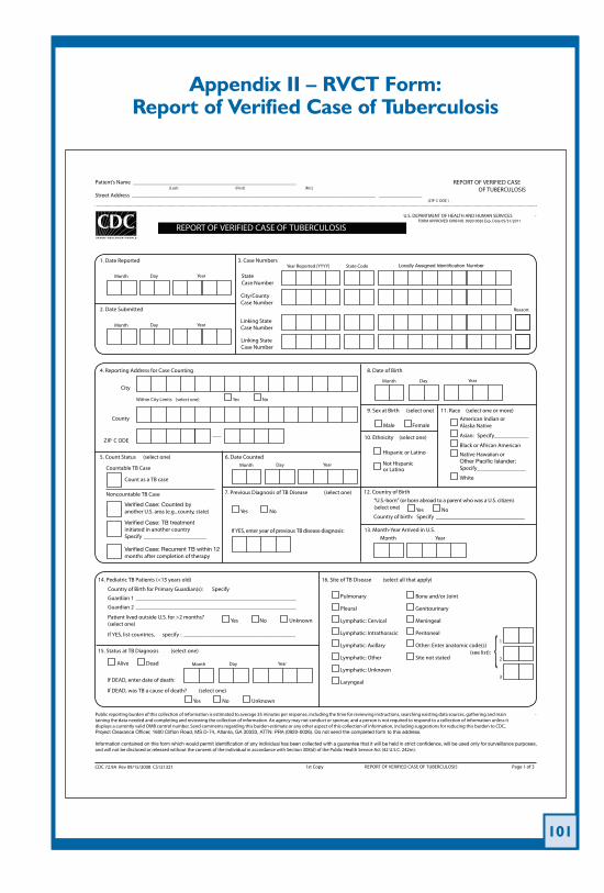
101
Appendix II – RVCT Form: Report of Verified Case of Tuberculosis
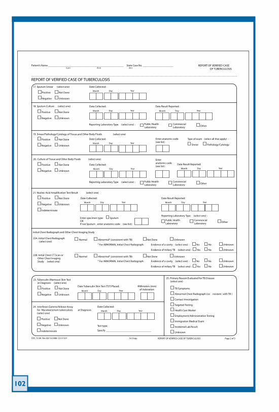
102
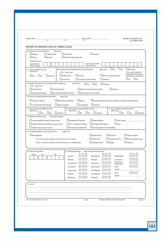
103
104
105
106
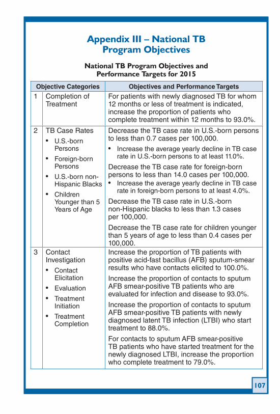
107
Appendix III – National TB Program Objectives
National TB Program Objectives and Performance Targets for 2015
Objective Categories Objectives and Performance Targets
1 Completion of Treatment
For patients with newly diagnosed TB for whom 12 months or less of treatment is indicated, increase the proportion of patients who complete treatment within 12 months to 93.0%.
2 TB Case Rates
U.S.-born •Persons
Foreign-born •Persons
U.S.-born non-•Hispanic Blacks
Children •Younger than 5 Years of Age
Decrease the TB case rate in U.S.-born persons to less than 0.7 cases per 100,000.
Increase the average yearly decline in TB case •rate in U.S.-born persons to at least 11.0%.
Decrease the TB case rate for foreign-born persons to less than 14.0 cases per 100,000.
Increase the average yearly decline in TB case •rate in foreign-born persons to at least 4.0%.
Decrease the TB case rate in U.S.-born non-Hispanic blacks to less than 1.3 cases per 100,000.
Decrease the TB case rate for children younger than 5 years of age to less than 0.4 cases per 100,000.
3 Contact Investigation
Contact •Elicitation
Evaluation•Treatment •Initiation
Treatment •Completion
Increase the proportion of TB patients with positive acid-fast bacillus (AFB) sputum-smear results who have contacts elicited to 100.0%.
Increase the proportion of contacts to sputum AFB smear-positive TB patients who are evaluated for infection and disease to 93.0%.
Increase the proportion of contacts to sputum AFB smear-positive TB patients with newly diagnosed latent TB infection (LTBI) who start treatment to 88.0%.
For contacts to sputum AFB smear-positive TB patients who have started treatment for the newly diagnosed LTBI, increase the proportion who complete treatment to 79.0%.
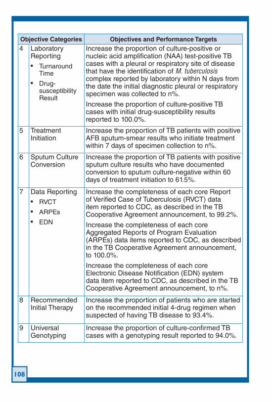
108
Objective Categories Objectives and Performance Targets
4 Laboratory Reporting
Turnaround •Time
Drug-•susceptibility Result
Increase the proportion of culture-positive or nucleic acid amplification (NAA) test-positive TB cases with a pleural or respiratory site of disease that have the identification of M. tuberculosis complex reported by laboratory within N days from the date the initial diagnostic pleural or respiratory specimen was collected to n%.
Increase the proportion of culture-positive TB cases with initial drug-susceptibility results reported to 100.0%.
5 Treatment Initiation
Increase the proportion of TB patients with positive AFB sputum-smear results who initiate treatment within 7 days of specimen collection to n%.
6 Sputum Culture Conversion
Increase the proportion of TB patients with positive sputum culture results who have documented conversion to sputum culture-negative within 60 days of treatment initiation to 61.5%.
7 Data Reporting
RVCT•ARPEs•EDN •
Increase the completeness of each core Report of Verified Case of Tuberculosis (RVCT) data item reported to CDC, as described in the TB Cooperative Agreement announcement, to 99.2%.
Increase the completeness of each core Aggregated Reports of Program Evaluation (ARPEs) data items reported to CDC, as described in the TB Cooperative Agreement announcement, to 100.0%.
Increase the completeness of each core Electronic Disease Notification (EDN) system data item reported to CDC, as described in the TB Cooperative Agreement announcement, to n%.
8 Recommended Initial Therapy
Increase the proportion of patients who are started on the recommended initial 4-drug regimen when suspected of having TB disease to 93.4%.
9 Universal Genotyping
Increase the proportion of culture-confirmed TB cases with a genotyping result reported to 94.0%.
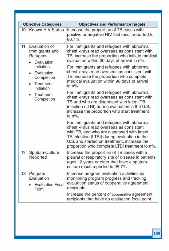
109
Objective Categories Objectives and Performance Targets10 Known HIV Status Increase the proportion of TB cases with
positive or negative HIV test result reported to 88.7%.
11 Evaluation of Immigrants and Refugees
Evaluation •Initiation
Evaluation •Completion
Treatment •Initiation
Treatment •Completion
For immigrants and refugees with abnormal chest x-rays read overseas as consistent with TB, increase the proportion who initiate medical evaluation within 30 days of arrival to n%.
For immigrants and refugees with abnormal chest x-rays read overseas as consistent with TB, increase the proportion who complete medical evaluation within 90 days of arrival to n%.
For immigrants and refugees with abnormal chest x-rays read overseas as consistent with TB and who are diagnosed with latent TB infection (LTBI) during evaluation in the U.S., increase the proportion who start treatment to n%.
For immigrants and refugees with abnormal chest x-rays read overseas as consistent with TB, and who are diagnosed with latent TB infection (LTBI) during evaluation in the U.S. and started on treatment, increase the proportion who complete LTBI treatment to n%.
12 Sputum-Culture Reported
Increase the proportion of TB cases with a pleural or respiratory site of disease in patients ages 12 years or older that have a sputum-culture result reported to 95.7%.
13 Program Evaluation
Evaluation Focal •Point
Increase program evaluation activities by monitoring program progress and tracking evaluation status of cooperative agreement recipients.
Increase the percent of cooperative agreement recipients that have an evaluation focal point.
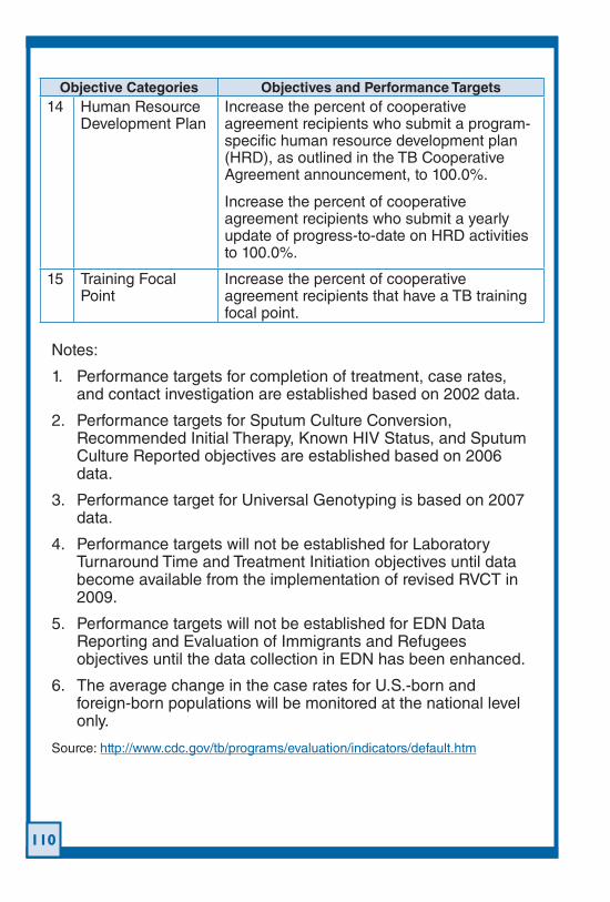
110
Objective Categories Objectives and Performance Targets14 Human Resource
Development Plan Increase the percent of cooperative agreement recipients who submit a program-specific human resource development plan (HRD), as outlined in the TB Cooperative Agreement announcement, to 100.0%.
Increase the percent of cooperative agreement recipients who submit a yearly update of progress-to-date on HRD activities to 100.0%.
15 Training Focal Point
Increase the percent of cooperative agreement recipients that have a TB training focal point.
Notes:
Performance targets for completion of treatment, case rates, 1. and contact investigation are established based on 2002 data.
Performance targets for Sputum Culture Conversion, 2. Recommended Initial Therapy, Known HIV Status, and Sputum Culture Reported objectives are established based on 2006 data.
Performance target for Universal Genotyping is based on 2007 3. data.
Performance targets will not be established for Laboratory 4. Turnaround Time and Treatment Initiation objectives until data become available from the implementation of revised RVCT in 2009.
Performance targets will not be established for EDN Data 5. Reporting and Evaluation of Immigrants and Refugees objectives until the data collection in EDN has been enhanced.
The average change in the case rates for U.S.-born and 6. foreign-born populations will be monitored at the national level only.
Source: http://www.cdc.gov/tb/programs/evaluation/indicators/default.htm
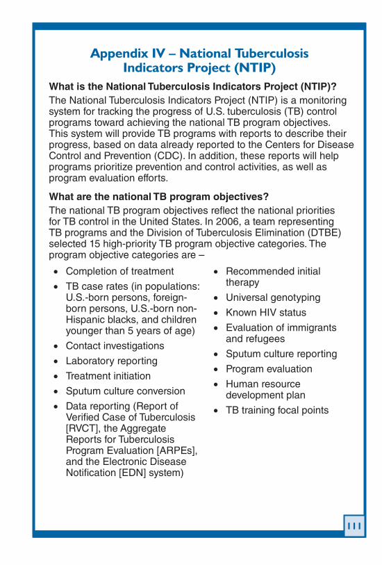
111
Appendix IV – National Tuberculosis Indicators Project (NTIP)
What is the National Tuberculosis Indicators Project (NTIP)?The National Tuberculosis Indicators Project (NTIP) is a monitoring system for tracking the progress of U.S. tuberculosis (TB) control programs toward achieving the national TB program objectives. This system will provide TB programs with reports to describe their progress, based on data already reported to the Centers for Disease Control and Prevention (CDC). In addition, these reports will help programs prioritize prevention and control activities, as well as program evaluation efforts.
What are the national TB program objectives?The national TB program objectives reflect the national priorities for TB control in the United States. In 2006, a team representing TB programs and the Division of Tuberculosis Elimination (DTBE) selected 15 high-priority TB program objective categories. The program objective categories are –
Completion of treatment•TB case rates (in populations: •U.S.-born persons, foreign-born persons, U.S.-born non-Hispanic blacks, and children younger than 5 years of age)
Contact investigations•Laboratory reporting•Treatment initiation•Sputum culture conversion•Data reporting (Report of •Verified Case of Tuberculosis [RVCT], the Aggregate Reports for Tuberculosis Program Evaluation [ARPEs], and the Electronic Disease Notification [EDN] system)
Recommended initial •therapy
Universal genotyping•Known HIV status•Evaluation of immigrants •and refugees
Sputum culture reporting•Program evaluation•Human resource •development plan
TB training focal points•
112
TB programs funded through cooperative agreements will be expected to report on their progress toward achieving all 15 national TB program objective categories starting in 2010.
Why was NTIP undertaken?Program evaluation is an essential component of an effective public health program. Since 2005, DTBE has included program evaluation as a core requirement of the cooperative agreement. With the understanding of the resource limitations and constraints faced by TB programs, NTIP was developed to facilitate the use of existing data to help programs prioritize activities and focus program evaluation efforts.
Who was involved and how was the system developed?The design of NTIP reports is modeled after the Tuberculosis Indicators Project (TIP), developed by the California Department of Health. To validate the selected national objectives and standardize the measurements for tracking progress toward the objectives, a team of DTBE and TB control program staff from Colorado, New York State, Minnesota, and Tennessee worked together and discussed the validity, reliability, and accuracy of the measures, as well as how the measures will impact programs. The group designed reporting templates to provide information that is significant and programmatically relevant. Representatives from the National Tuberculosis Controllers Association (NTCA), the Advisory Council for the Elimination of Tuberculosis (ACET), the TB Education and Training Network (TB ETN), the Evaluation Working Group (EWG), and other interested TB programs were invited to a 2-day intensive review meeting to further validate the indicators and to provide input and guidance on their development.
How will NTIP affect TB control programs?NTIP provides a standardized method for calculating indicators and tracking program progress across sites and over time, thus enabling DTBE’s and programs’ abilities to assess the impact of TB control efforts locally as well as nationally. In the past, programs calculated their own performance indices and reported progress to CDC. Variations in the calculations have hindered our abilities to observe and compare performance from one year to another, and to track progress over time.
113
Unlike the annual national surveillance report (Reported Tuberculosis in the United States) published by CDC, NTIP will provide each program with an individualized report of their performance, based on the data submitted by the programs to CDC. The reports will include the national TB program objectives and national performance targets as guidance. Working closely with DTBE program consultants, program areas will be able to continue to set their own performance targets based on what is feasible, as well as compare their performance to the national average.TB programs will use NTIP to track and report progress toward achieving national objectives as a part of the cooperative agreement reporting requirements (i.e., annual and interim progress reports) in 2010. Program areas will be required to provide justifications on objectives for which they did not meet the performance targets, and to provide an evaluation plan for one objective selected in consultation with DTBE consultants.
What TB programs need to do to use this system?NTIP reports will be provided to all cooperative agreement recipients (i.e., TB programs) as a service from DTBE. NTIP utilizes data that are currently being reported to DTBE via the Report of Verified Case of Tuberculosis (RVCT), the Aggregate Reports for Tuberculosis Program Evaluation (ARPEs) on contacts, and the Electronic Disease Notification (EDN) system for the follow-up evaluation of immigrants and refugees with a B notification. TB programs will not have to do any additional work or collect any additional data to generate NTIP reports.
When will NTIP be implemented?A selected number of preliminary NTIP reports will be available to cooperative agreement recipients starting in the fall of 2008 (i.e., completion of treatment, TB case rates, contact investigation, laboratory reporting [drug-susceptibility results], sputum culture conversion, data reporting, recommended initial therapy, known HIV status, evaluation of immigrants and refugees with a B notification, and sputum culture reporting, and universal genotyping). Indicator reports calculated using new RVCT variables (e.g., treatment initiation and laboratory reporting [turn-around time]) will be available after the implementation of the revised RVCT.
NTIP will be expected to include current data as they are submitted to CDC after the implementation of the revised RVCT and the software that will replace the Tuberculosis Information Management
114
System (TIMS). NTIP will also be expected to provide reports for some high-incidence counties that are not direct recipients of cooperative agreement in the future. Guidance on the reporting requirement for the national TB program objectives and the use of NTIP reports for counties will be established by their respective state TB program offices.
Additional ResourcesCDC. National Tuberculosis Indicators Project (NTIP): Frequently Asked Questions. Retrieved from: www.cdc.gov/tb/publications/factsheets/statistics/NTIPFAQs.htm
CDC. TB Program Evaluation Handbook. Retrieved from: www.cdc.gov/tb/programs/Evaluation/TBEvaluationHandbook_tagged.pdf
CDC. A Guide to Developing a TB Program Evaluation Plan www.cdc.gov/tb/programs/Evaluation/guide.htm
Source: http://www.cdc.gov/tb/publications/factsheets/statistics/NTIP.htm
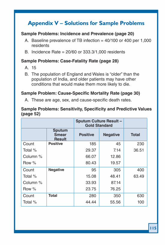
115
Appendix V – Solutions for Sample Problems
Sample Problems: Incidence and Prevalence (page 20)
A. Baseline prevalence of TB infection = 40/100 or 400 per 1,000 residents
B. Incidence Rate = 20/60 or 333.3/1,000 residents
Sample Problems: Case-Fatality Rate (page 28)
A. 15
B. The population of England and Wales is “older” than the population of India, and older patients may have other conditions that would make them more likely to die.
Sample Problem: Cause-Specific Mortality Rate (page 30)
A. These are age, sex, and cause-specific death rates.
Sample Problems: Sensitivity, Specificity and Predictive Values (page 52)
Sputum Culture Result – Gold Standard
Sputum Smear Result
Positive Negative Total
Count
Total %
Column %
Row %
Positive 185
29.37
66.07
80.43
45
7.14
12.86
19.57
230
36.51
Count
Total %
Column %
Row %
Negative 95
15.08
33.93
23.75
305
48.41
87.14
76.25
400
63.49
Count
Total %
Total 280
44.44
350
55.56
630
100
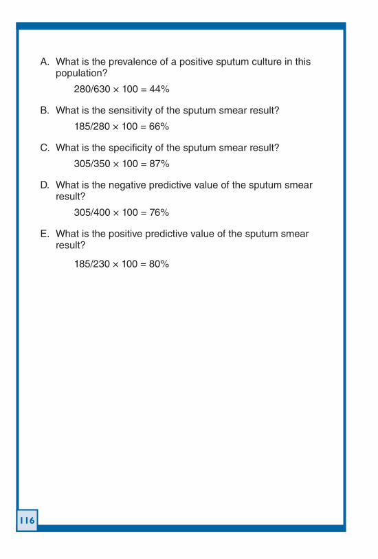
116
A. What is the prevalence of a positive sputum culture in this population?
280/630 × 100 = 44%
B. What is the sensitivity of the sputum smear result?
185/280 × 100 = 66%
C. What is the specificity of the sputum smear result?
305/350 × 100 = 87%
D. What is the negative predictive value of the sputum smear result?
305/400 × 100 = 76%
E. What is the positive predictive value of the sputum smear result?
185/230 × 100 = 80%
117
Appendix VI – Suggested Reading ListCenters for Disease Control and Prevention, Excellence in Curriculum Integration through Teaching Epidemiology (EXCITE) Website. Retrieved from: http://www.cdc.gov/excite/index.htm
Gordis L. Epidemiology. 4th ed. New York: W. B. Saunders Company; 2009.
Greenberg R. Medical Epidemiology. 4th ed. New York: Lange Medical Books. McGraw-Hill; 2004.
Haupt A, Kane TT, Haub C. PRB’s Population Handbook. 6th ed. 2011. Retrieved from http://www.prb.org/pdf11/prb-population-handbook-2011.pdf
Holland, B. Probability Without Equations: Concepts for Clinicians. Baltimore, MD: The Johns Hopkins University Press, 1997.
Lillienfeld DE, Stolley, PD. Foundations of Epidemiology. 3rd ed. New York, NY: Oxford University Press; 1994.
National TB Controllers Association/CDC Advisory Group on TB Genotyping. Guide to the Application of Genotyping to Tuberculosis Prevention and Control. Atlanta, GA: United States Department of Health and Human Services, CDC; June 2004. Retrieved from http://www.cdc.gov/tb/programs/genotyping/manual.htm
118
Additional TB ResourcesCenters for Disease Control and Prevention (CDC) Division of Tuberculosis Elimination www.cdc.gov/tb
The CDC Division of Tuberculosis Elimination’s website contains information on TB in the United States and provides TB education and training materials and resources.
Find TB Resources Website www.findtbresources.org
This website includes a searchable database of materials from numerous national and international organizations. The site also includes information about other TB organizations, how to order materials, and funding opportunities.
TB Regional Training and Medical Consultation Centers (RTMCCs)
CDC’s Division of Tuberculosis Elimination funds regional RTMCCs to provide tuberculosis training, education and medical consultation services within their assigned region. More information on the RTMCCs can be found at: www.cdc.gov/tb/education/rtmc/
The RTMCC All Products webpage provides access to all RTMCC-produced TB educational materials and is available at: http://sntc.medicine.ufl.edu/rtmccproducts.aspx


New Jersey Medical School Global Tuberculosis Institute (GTBI)225 Warren Street
P.O. Box 1709Newark, NJ 07101-1709www.umdnj.edu/globaltb
Related Documents