Basic Applied Finite Element Analysis · Plate Element Model of a Thin-Walled Bottle Under Pressure • 3D Solid Element Models: Most commonly used for bulky or chunky parts with

PDHonline Course G180 (8 PDH)

Basic Applied Finite Element Analysis

2012

Instructor: Robert B. Wilcox, P.E.

PDH Online | PDH Center5272 Meadow Estates Drive

Fairfax, VA 22030-6658Phone & Fax: 703-988-0088

www.PDHonline.orgwww.PDHcenter.com

An Approved Continuing Education Provider

http://www.PDHonline.org

http://www.PDHcenter.com

www.PDHcenter.com PDH Course G180 www.PDHonline.org

Page 1 of 19

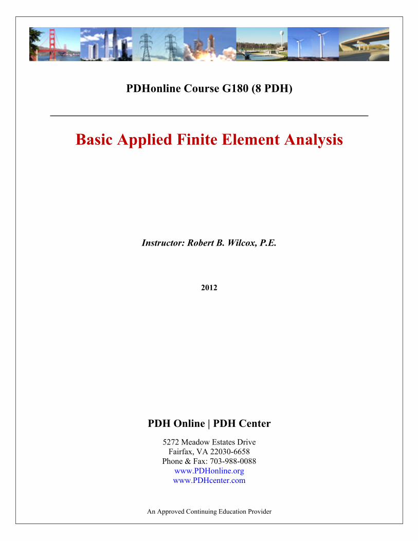
Basic Linear Static Finite Element Analysis

Robert B. Wilcox, P.E.

Prerequisites to Applying Linear Static FEA Before applying the method of FEA, it is important that the analyst has a clear understanding of statics and strength of materials concepts. It is not the intent of this course to cover these topics, but rather, to allow one having an understanding of these topics to be able to apply them using FEA. So before applying FEA, it may be a good idea to review the basics of these subjects. Some of the concepts you should be familiar with include:

• Static Equilibrium • Moments of Inertia • Axial Loading, Pressure, Bending, Torsion • Stress and Strain • Basic Material Properties • Stress Concentration • Basic Failure Theory

mailto:[email protected]


Page 2 of 19

The analyst who has a solid working knowledge in these areas will be much better equipped to define the problem correctly, which is more than half the battle in practical application of FEA. Definitions Some of the vocabulary particular to FEA:

• Node: An individual point in the model. • Element: A piece of the model structure, bounded by nodes. • Stiffness Matrix: The mathematic representation of the model's deflection response to applied

loads. • Degree of Freedom: The ability of a node to translate or rotate in space. A node may have up

to six degrees of freedom, three translational, and three rotational. • Boundary Conditions: Constraints or loads applied through nodes on the model. • Mesh: The collection of nodes and elements which define the model, displayed graphically • Pre-processor: The portion of a program used to define the geometry, boundary conditions,

and material properties of the model. Geometry is frequently defined in a separate CAD program with solid modeling capabilities, then passed to the FEA program for meshing.

• Solver: The portion of the FEA program which actually calculates the displacements and stresses for the problem model.

• Post-processor: The portion of the code which allows for viewing and outputting the results of the analysis, such as contour (fringe) plots of stress magnitude, displacements, or reaction forces.

Important Assumptions of Linear Static FEA Linear static models are based on some basic assumptions which may or may not be correct for the problem at hand. Understanding these assumptions will allow the analyst to decide if linear static FEA is appropriate for solving the problem. The most important assumptions are:

• Loads are applied gradually and do not change over time. If effects due to dynamic loading are to be considered, such as impact, resonance, random vibration, time-varying magnitude or direction - then a linear static modeling approach will be a poor assumption.

• Displacements are relatively small. • Boundary conditions accurately represent the state of loads and supports. This is an area to

pay particular attention to when modeling. How constraints and loads are applied can radically affect the results in terms of deflection and stress output.

• Linear material assumptions are valid. The material must obey Hooke's law for linear FEA modeling to be valid. For example, if yield strength of the material is exceeded in the model, then the model is not longer valid from a linear perspective. The key variable is usually the elastic modulus for the material and it is considered constant in linear analysis.

• Model is stable and satisfies static equilibrium: No rigid body movements, mechanism actions, etc. will be tolerated by linear FEA codes. Only deflections due to stresses imposed on the parts should occur.

• Stress stiffening effects are minimal. This is a fairly difficult to predict phenomenon in which a particular geometry will become stiffer or less stiff as it deflects. If membrane stresses coupled with bending are significant, stress stiffening may be an issue and non-linear methods may be needed for the solution.

Basic Analysis Types


Page 3 of 19

Linear static analysis types may be roughly divided into two broad categories - 3D and planar: 3D analysis types may be further broken down into three main categories:

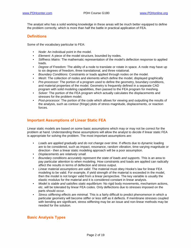
• Beam Models: Beam elements are frequently used in structural analysis. There are two main types of beam elements - those which support bending moments at the end, and those which do not (truss elements). Beam elements are assigned section properties and coordinate systems and generally are connected by nodes at each end. Beam models may be spatial (3-D) or planar , like the one below.

Truss Element Model

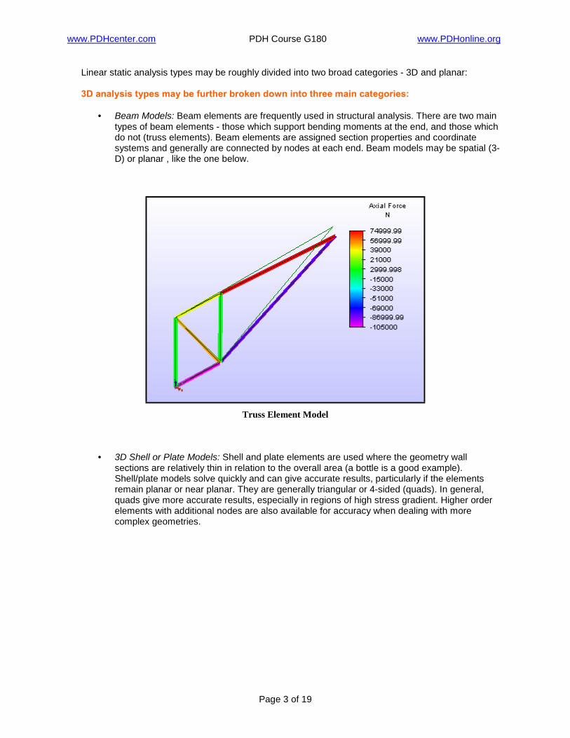
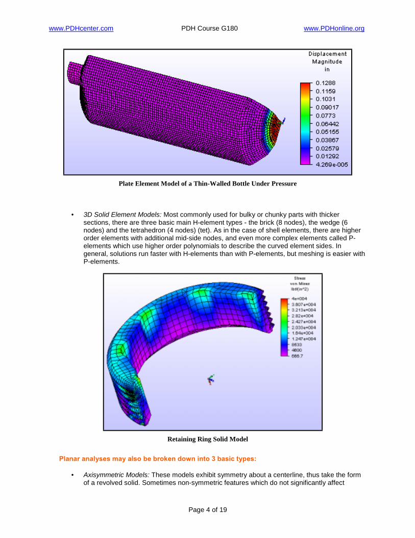
• 3D Shell or Plate Models: Shell and plate elements are used where the geometry wall sections are relatively thin in relation to the overall area (a bottle is a good example). Shell/plate models solve quickly and can give accurate results, particularly if the elements remain planar or near planar. They are generally triangular or 4-sided (quads). In general, quads give more accurate results, especially in regions of high stress gradient. Higher order elements with additional nodes are also available for accuracy when dealing with more complex geometries.


Page 4 of 19

Plate Element Model of a Thin-Walled Bottle Under Pressure

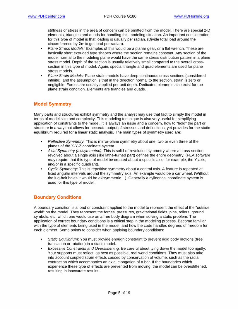
• 3D Solid Element Models: Most commonly used for bulky or chunky parts with thicker sections, there are three basic main H-element types - the brick (8 nodes), the wedge (6 nodes) and the tetrahedron (4 nodes) (tet). As in the case of shell elements, there are higher order elements with additional mid-side nodes, and even more complex elements called P-elements which use higher order polynomials to describe the curved element sides. In general, solutions run faster with H-elements than with P-elements, but meshing is easier with P-elements.

Retaining Ring Solid Model

Planar analyses may also be broken down into 3 basic types:

• Axisymmetric Models: These models exhibit symmetry about a centerline, thus take the form of a revolved solid. Sometimes non-symmetric features which do not significantly affect


Page 5 of 19

stiffness or stress in the area of concern can be omitted from the model. There are special 2-D elements, triangles and quads for handling this modeling situation. An important consideration for this type of model is that loading is usually per radian. (Divide total load around the circumference by 2π to get load per radian).

• Plane Stress Models: Examples of this would be a planar gear, or a flat wrench. These are basically short extruded type shapes where the section remains constant. Any section of the model normal to the modeling plane would have the same stress distribution pattern in a plane stress model. Depth of the section is usually relatively small compared to the overall cross-section in this type of model. Again, special triangle and quad elements are used for plane stress models.

• Plane Strain Models: Plane strain models have deep continuous cross-sections (considered infinite), and the assumption is that in the direction normal to the section, strain is zero or negligible. Forces are usually applied per unit depth. Dedicated elements also exist for the plane strain condition. Elements are triangles and quads.

Model Symmetry Many parts and structures exhibit symmetry and the analyst may use that fact to simply the model in terms of model size and complexity. This modeling technique is also very useful for simplifying application of constraints to the model. It is always an issue and a concern, how to "hold" the part or structure in a way that allows for accurate output of stresses and deflections, yet provides for the static equilibrium required for a linear static analysis. The main types of symmetry used are:

• Reflective Symmetry: This is mirror-plane symmetry about one, two or even three of the planes of the X-Y-Z coordinate system.

• Axial Symmetry (axisymmetric): This is solid-of-revolution symmetry where a cross-section revolved about a single axis (like lathe-turned part) defines the entire geometry. (FEA software may require that this type of model be created about a specific axis, for example, the Y-axis, and/or in a specific quadrant).

• Cyclic Symmetry: This is repetitive symmetry about a central axis. A feature is repeated at fixed angular intervals around the symmetry axis. An example would be a car wheel. (Without the lug-bolt holes it would be axisymmetric…). Generally a cylindrical coordinate system is used for this type of model.

Boundary Conditions A boundary condition is a load or constraint applied to the model to represent the effect of the "outside world" on the model. They represent the forces, pressures, gravitational fields, pins, rollers, ground symbols, etc. which one would use on a free body diagram when solving a static problem. The application of correct boundary conditions is a critical step in the modeling process. Become familiar with the type of elements being used in the model, and how the code handles degrees of freedom for each element. Some points to consider when applying boundary conditions:

• Static Equilibrium: You must provide enough constraint to prevent rigid body motions (free translation or rotation) in a static model.

• Excessive Constraints and Overstiffening: Be careful about tying down the model too rigidly. Your supports must reflect, as best as possible, real world conditions. They must also take into account coupled strain effects caused by conservation of volume, such as the radial contraction which accompanies an axial elongation of a bar. If the boundaries which experience these type of effects are prevented from moving, the model can be overstiffened, resulting in inaccurate results.


Page 6 of 19

• Point Loads: Loads applied at a single point may cause unreasonably high local stress and deformation. Most real world loads are not applied to a single point, so try to give some thought to how the actual load is applied and simulate it with distributed loads, pressures, etc. if possible.

• Symmetry Constraints: If there is a plane of symmetry, it can be assumed there will be no translation of the nodes in the direction normal to the plane of symmetry. Rotational degrees of freedom may also have to be considered to keep shell elements from pivoting, for example.

Problem Solving Methodology The first model will be a simple rectangular plate with a round hole. Stress concentration effects of this geometry are well documented so results are easily verifiable. In general, the following general steps will be followed when setting up and solving an FEA problem:

• Model the Geometry: This is essentially drawing or modeling the part. This can be done within some FEA codes, and others allow import of CAD geometry. We'll be creating our part right in the demo FEA program.

• Generate the Mesh: Creation of the nodes and elements which follow the geometry created. If this is done automatically it is called "automeshing". This is the method we will use. (Another method called "structured meshing" may be preferred for some problems. More on Structured meshing later…).

• Define Material Properties: This is simply specifying the material properties and in many cases with modern codes, it is simply a matter of choosing the material from a database. Key properties are the elastic modulus, mass density and the poisson's ratio.

• Define Loads and Boundary Conditions: This is specifying the applied forces and the supports (constraints) to the model.

• Reality Checks: A crucial step - predicting some key parameters with hand calculations. • Solve: This is running the actual code to solve for displacements, stresses and reactions. • View and Interpret Results: Usually viewing contour plots of stress and displacement levels,

examining deformed geometry plots, and checking element quality and precision of results. • Verification: This step includes checking element shape and quality, von Mises precision, and

viewing unsmoothed vs. smoothed fringe plots. (The demonstration software does not support these features. Most full-featured commercial programs, however, will allow for these steps to be performed).

• Refinement and Convergence: The step nobody talks about! Many times several runs are needed to achieve reliable results, and there is a definite method to mesh refinement and convergence to an accurate solution.

Download and Install FEA Code and Example Files The method of this course is learning by example and practice. So right from the outset, it would be a good idea to download and install the FEA code. This is a trial version with node limit and limited features, and requires a PC with internet access. If you cannot download and install this code, you may follow along with the examples in the text. You will have a much more meaningful learning experience, however, if you run the code alongside the text as we proceed. Please download and install this demo version and example files by following this link: Demo Software and Example Files Page Follow the instructions on the link page to download and install the program. It is recommended that you do the first tutorial exercise included with the program prior to proceeding with the example. (Any


Page 7 of 19

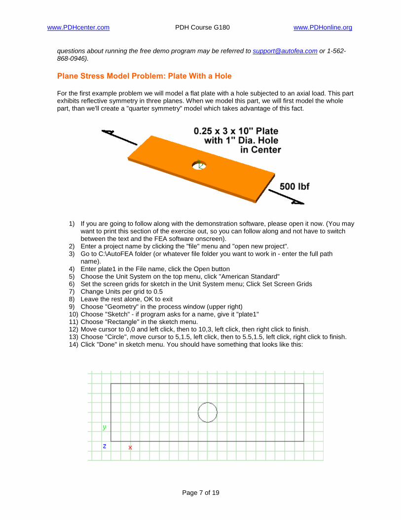
questions about running the free demo program may be referred to [email protected] or 1-562-868-0946). Plane Stress Model Problem: Plate With a Hole For the first example problem we will model a flat plate with a hole subjected to an axial load. This part exhibits reflective symmetry in three planes. When we model this part, we will first model the whole part, than we'll create a "quarter symmetry" model which takes advantage of this fact.

1) If you are going to follow along with the demonstration software, please open it now. (You may want to print this section of the exercise out, so you can follow along and not have to switch between the text and the FEA software onscreen).

2) Enter a project name by clicking the "file" menu and "open new project". 3) Go to C:\AutoFEA folder (or whatever file folder you want to work in - enter the full path

name). 4) Enter plate1 in the File name, click the Open button 5) Choose the Unit System on the top menu, click "American Standard" 6) Set the screen grids for sketch in the Unit System menu; Click Set Screen Grids 7) Change Units per grid to 0.5 8) Leave the rest alone, OK to exit 9) Choose "Geometry" in the process window (upper right) 10) Choose "Sketch" - if program asks for a name, give it "plate1" 11) Choose "Rectangle" in the sketch menu. 12) Move cursor to 0,0 and left click, then to 10,3, left click, then right click to finish. 13) Choose "Circle", move cursor to 5,1.5, left click, then to 5.5,1.5, left click, right click to finish. 14) Click "Done" in sketch menu. You should have something that looks like this:

mailto:[email protected]


Page 8 of 19

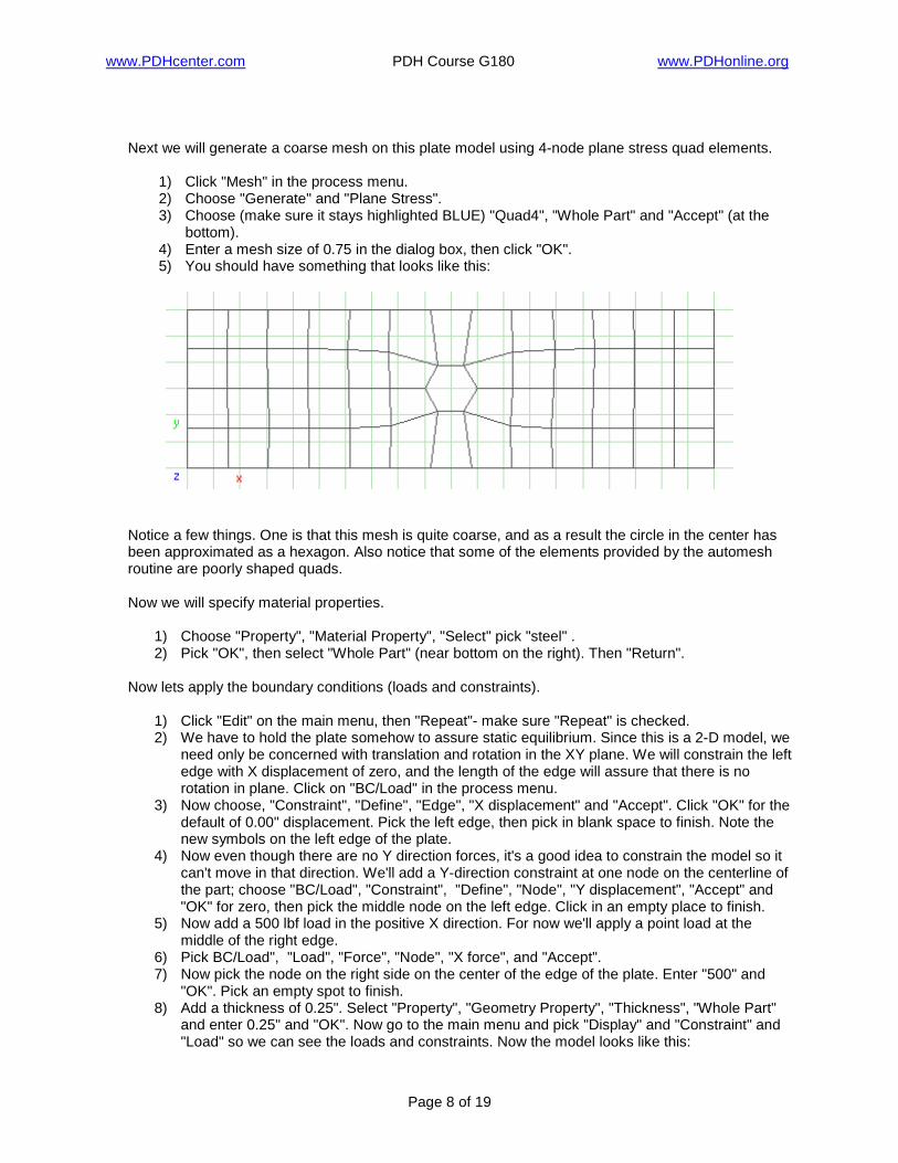
Next we will generate a coarse mesh on this plate model using 4-node plane stress quad elements.

1) Click "Mesh" in the process menu. 2) Choose "Generate" and "Plane Stress". 3) Choose (make sure it stays highlighted BLUE) "Quad4", "Whole Part" and "Accept" (at the

bottom). 4) Enter a mesh size of 0.75 in the dialog box, then click "OK". 5) You should have something that looks like this:

Notice a few things. One is that this mesh is quite coarse, and as a result the circle in the center has been approximated as a hexagon. Also notice that some of the elements provided by the automesh routine are poorly shaped quads. Now we will specify material properties.

1) Choose "Property", "Material Property", "Select" pick "steel" . 2) Pick "OK", then select "Whole Part" (near bottom on the right). Then "Return".

Now lets apply the boundary conditions (loads and constraints).

1) Click "Edit" on the main menu, then "Repeat"- make sure "Repeat" is checked. 2) We have to hold the plate somehow to assure static equilibrium. Since this is a 2-D model, we

need only be concerned with translation and rotation in the XY plane. We will constrain the left edge with X displacement of zero, and the length of the edge will assure that there is no rotation in plane. Click on "BC/Load" in the process menu.

3) Now choose, "Constraint", "Define", "Edge", "X displacement" and "Accept". Click "OK" for the default of 0.00" displacement. Pick the left edge, then pick in blank space to finish. Note the new symbols on the left edge of the plate.

4) Now even though there are no Y direction forces, it's a good idea to constrain the model so it can't move in that direction. We'll add a Y-direction constraint at one node on the centerline of the part; choose "BC/Load", "Constraint", "Define", "Node", "Y displacement", "Accept" and "OK" for zero, then pick the middle node on the left edge. Click in an empty place to finish.

5) Now add a 500 lbf load in the positive X direction. For now we'll apply a point load at the middle of the right edge.

6) Pick BC/Load", "Load", "Force", "Node", "X force", and "Accept". 7) Now pick the node on the right side on the center of the edge of the plate. Enter "500" and

"OK". Pick an empty spot to finish. 8) Add a thickness of 0.25". Select "Property", "Geometry Property", "Thickness", "Whole Part"

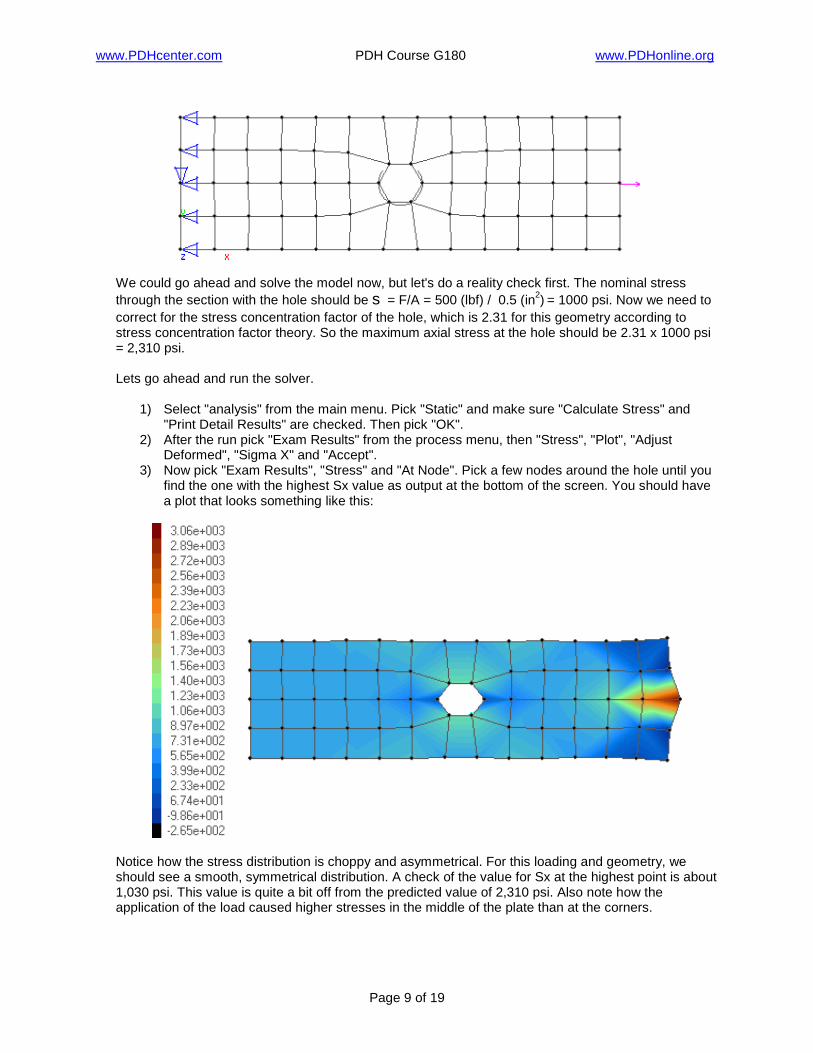
and enter 0.25" and "OK". Now go to the main menu and pick "Display" and "Constraint" and "Load" so we can see the loads and constraints. Now the model looks like this:


Page 9 of 19

We could go ahead and solve the model now, but let's do a reality check first. The nominal stress through the section with the hole should be s = F/A = 500 (lbf) / 0.5 (in2) = 1000 psi. Now we need to correct for the stress concentration factor of the hole, which is 2.31 for this geometry according to stress concentration factor theory. So the maximum axial stress at the hole should be 2.31 x 1000 psi = 2,310 psi. Lets go ahead and run the solver.

1) Select "analysis" from the main menu. Pick "Static" and make sure "Calculate Stress" and "Print Detail Results" are checked. Then pick "OK".

2) After the run pick "Exam Results" from the process menu, then "Stress", "Plot", "Adjust Deformed", "Sigma X" and "Accept".

3) Now pick "Exam Results", "Stress" and "At Node". Pick a few nodes around the hole until you find the one with the highest Sx value as output at the bottom of the screen. You should have a plot that looks something like this:

Notice how the stress distribution is choppy and asymmetrical. For this loading and geometry, we should see a smooth, symmetrical distribution. A check of the value for Sx at the highest point is about 1,030 psi. This value is quite a bit off from the predicted value of 2,310 psi. Also note how the application of the load caused higher stresses in the middle of the plate than at the corners.


Page 10 of 19

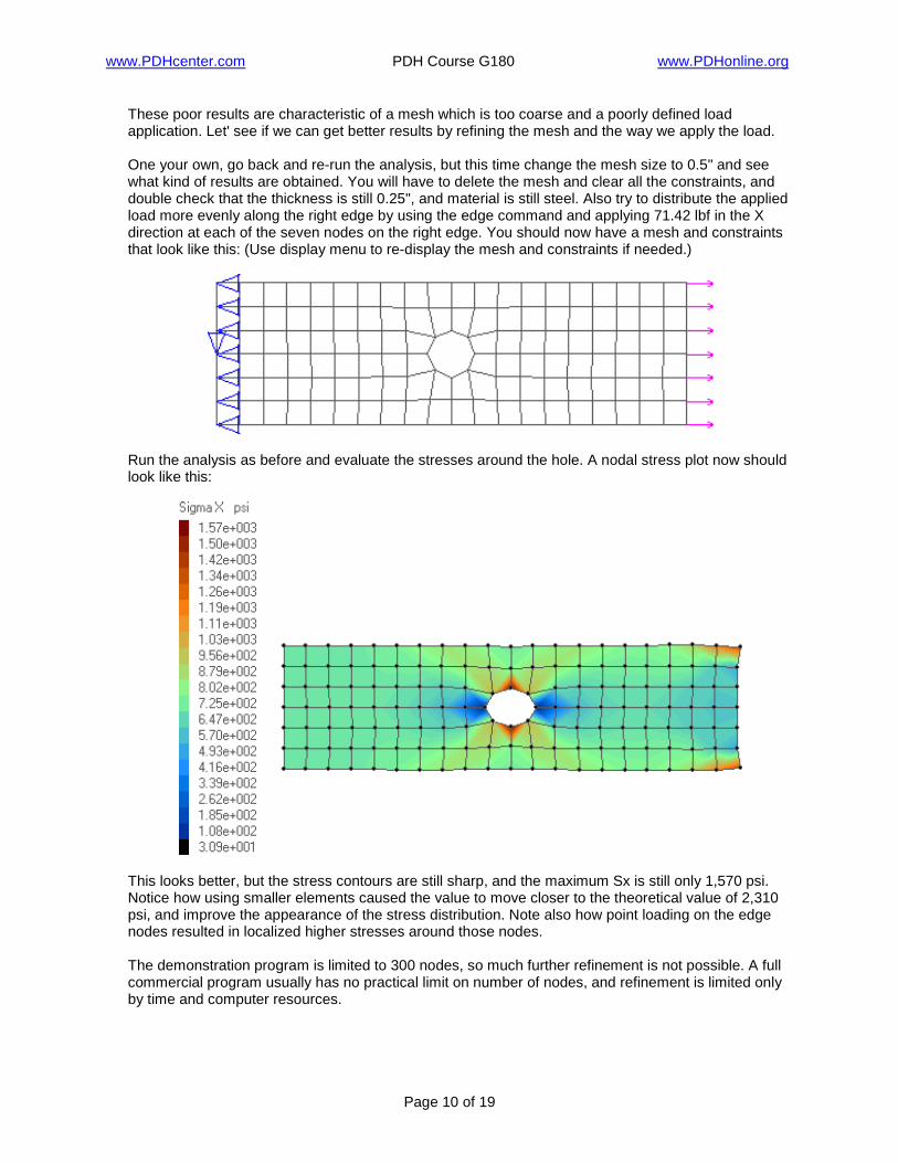
These poor results are characteristic of a mesh which is too coarse and a poorly defined load application. Let' see if we can get better results by refining the mesh and the way we apply the load. One your own, go back and re-run the analysis, but this time change the mesh size to 0.5" and see what kind of results are obtained. You will have to delete the mesh and clear all the constraints, and double check that the thickness is still 0.25", and material is still steel. Also try to distribute the applied load more evenly along the right edge by using the edge command and applying 71.42 lbf in the X direction at each of the seven nodes on the right edge. You should now have a mesh and constraints that look like this: (Use display menu to re-display the mesh and constraints if needed.)

Run the analysis as before and evaluate the stresses around the hole. A nodal stress plot now should look like this:

This looks better, but the stress contours are still sharp, and the maximum Sx is still only 1,570 psi. Notice how using smaller elements caused the value to move closer to the theoretical value of 2,310 psi, and improve the appearance of the stress distribution. Note also how point loading on the edge nodes resulted in localized higher stresses around those nodes. The demonstration program is limited to 300 nodes, so much further refinement is not possible. A full commercial program usually has no practical limit on number of nodes, and refinement is limited only by time and computer resources.


Page 11 of 19

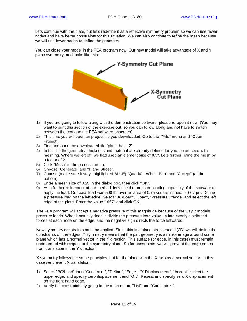
Lets continue with the plate, but let's redefine it as a reflective symmetry problem so we can use fewer nodes and have better constraints for this situation. We can also continue to refine the mesh because we will use fewer nodes to define the geometry. You can close your model in the FEA program now. Our new model will take advantage of X and Y plane symmetry, and looks like this:

1) If you are going to follow along with the demonstration software, please re-open it now. (You may

want to print this section of the exercise out, so you can follow along and not have to switch between the text and the FEA software onscreen).

2) This time you will open an project file you downloaded. Go to the "File" menu and "Open Project".

3) Find and open the downloaded file "plate_hole_2" 4) In this file the geometry, thickness and material are already defined for you, so proceed with

meshing. Where we left off, we had used an element size of 0.5". Lets further refine the mesh by a factor of 2.

5) Click "Mesh" in the process menu. 6) Choose "Generate" and "Plane Stress". 7) Choose (make sure it stays highlighted BLUE) "Quad4", "Whole Part" and "Accept" (at the

bottom). 8) Enter a mesh size of 0.25 in the dialog box, then click "OK". 9) As a further refinement of our method, let's use the pressure loading capability of the software to

apply the load. Our axial load was 500 lbf over an area of 0.75 square inches, or 667 psi. Define a pressure load on the left edge. Select "BC/Load", "Load", "Pressure", "edge" and select the left edge of the plate. Enter the value "-667" and click OK.

The FEA program will accept a negative pressure of this magnitude because of the way it models pressure loads. What it actually does is divide the pressure load value up into evenly distributed forces at each node on the edge, and the negative sign directs the force leftwards. Now symmetry constraints must be applied. Since this is a plane stress model (2D) we will define the constraints on the edges. Y symmetry means that the part geometry is a mirror image around some plane which has a normal vector in the Y direction. This surface (or edge, in this case) must remain undeformed with respect to the symmetry plane. So for constraints, we will prevent the edge nodes from translation in the Y direction. X symmetry follows the same principles, but for the plane with the X axis as a normal vector. In this case we prevent X translation.

1) Select "BC/Load" then "Constraint", "Define", "Edge", "Y Displacement", "Accept", select the

upper edge, and specify zero displacement and "OK". Repeat and specify zero X displacement on the right hand edge.

2) Verify the constraints by going to the main menu, "List" and "Constraints".


Page 12 of 19

3) Display the elements loads and constraints by going to the main menu, "display" and selecting loads, constraints, and mesh as necessary.

4) Your model should look like this now:

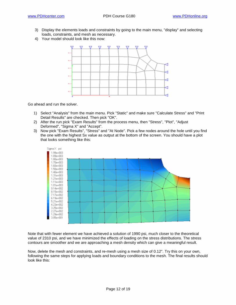
Go ahead and run the solver. 1) Select "Analysis" from the main menu. Pick "Static" and make sure "Calculate Stress" and "Print

Detail Results" are checked. Then pick "OK". 2) After the run pick "Exam Results" from the process menu, then "Stress", "Plot", "Adjust

Deformed", "Sigma X" and "Accept". 3) Now pick "Exam Results", "Stress" and "At Node". Pick a few nodes around the hole until you find

the one with the highest Sx value as output at the bottom of the screen. You should have a plot that looks something like this:

Note that with fewer element we have achieved a solution of 1990 psi, much closer to the theoretical value of 2310 psi, and we have minimized the effects of loading on the stress distributions. The stress contours are smoother and we are approaching a mesh density which can give a meaningful result.

Now, delete the mesh and constraints, and re-mesh using a mesh size of 0.12". Try this on your own, following the same steps for applying loads and boundary conditions to the mesh. The final results should look like this:


Page 13 of 19

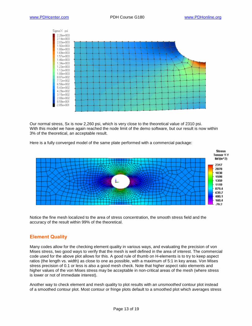
Our normal stress, Sx is now 2,260 psi, which is very close to the theoretical value of 2310 psi. With this model we have again reached the node limit of the demo software, but our result is now within 3% of the theoretical, an acceptable result. Here is a fully converged model of the same plate performed with a commercial package:

Notice the fine mesh localized to the area of stress concentration, the smooth stress field and the accuracy of the result within 99% of the theoretical. Element Quality Many codes allow for the checking element quality in various ways, and evaluating the precision of von Mises stress, two good ways to verify that the mesh is well defined in the area of interest. The commercial code used for the above plot allows for this. A good rule of thumb on H-elements is to try to keep aspect ratios (the length vs. width) as close to one as possible, with a maximum of 5:1 in key areas. Von Mises stress precision of 0.1 or less is also a good mesh check. Note that higher aspect ratio elements and higher values of the von Mises stress may be acceptable in non-critical areas of the mesh (where stress is lower or not of immediate interest). Another way to check element and mesh quality to plot results with an unsmoothed contour plot instead of a smoothed contour plot. Most contour or fringe plots default to a smoothed plot which averages stress


Page 14 of 19

or other output values across element boundaries to give a more continuous look to the plot. When viewing an unsmoothed plot, look for major breaks or discontinuities across element boundaries, which can indicate mesh problem areas or poorly shaped elements which may need further refinement. If the mesh is good, even an unsmoothed contour plot should look fairly continuous in critical areas especially. Structured Vs. Unstructured Meshes

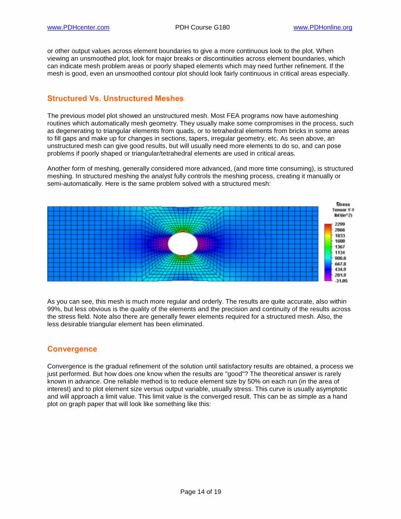
The previous model plot showed an unstructured mesh. Most FEA programs now have automeshing routines which automatically mesh geometry. They usually make some compromises in the process, such as degenerating to triangular elements from quads, or to tetrahedral elements from bricks in some areas to fill gaps and make up for changes in sections, tapers, irregular geometry, etc. As seen above, an unstructured mesh can give good results, but will usually need more elements to do so, and can pose problems if poorly shaped or triangular/tetrahedral elements are used in critical areas. Another form of meshing, generally considered more advanced, (and more time consuming), is structured meshing. In structured meshing the analyst fully controls the meshing process, creating it manually or semi-automatically. Here is the same problem solved with a structured mesh:

As you can see, this mesh is much more regular and orderly. The results are quite accurate, also within 99%, but less obvious is the quality of the elements and the precision and continuity of the results across the stress field. Note also there are generally fewer elements required for a structured mesh. Also, the less desirable triangular element has been eliminated. Convergence

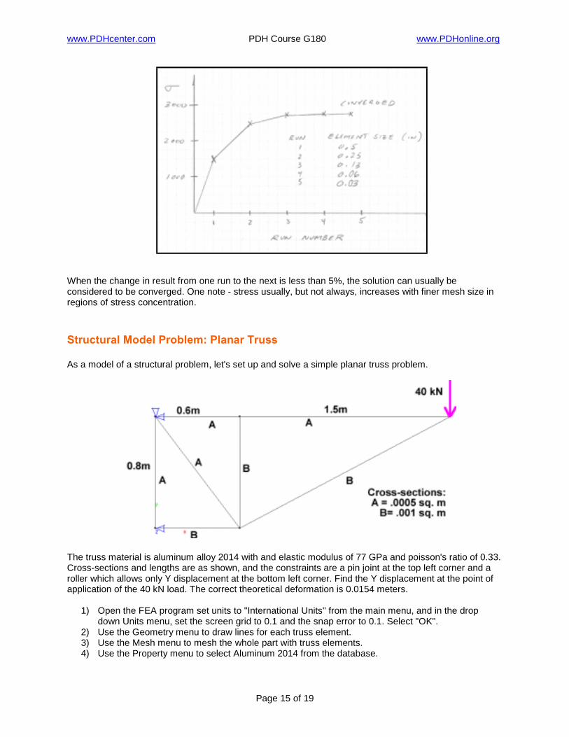
Convergence is the gradual refinement of the solution until satisfactory results are obtained, a process we just performed. But how does one know when the results are "good"? The theoretical answer is rarely known in advance. One reliable method is to reduce element size by 50% on each run (in the area of interest) and to plot element size versus output variable, usually stress. This curve is usually asymptotic and will approach a limit value. This limit value is the converged result. This can be as simple as a hand plot on graph paper that will look like something like this:


Page 15 of 19

When the change in result from one run to the next is less than 5%, the solution can usually be considered to be converged. One note - stress usually, but not always, increases with finer mesh size in regions of stress concentration.

Structural Model Problem: Planar Truss

As a model of a structural problem, let's set up and solve a simple planar truss problem.

The truss material is aluminum alloy 2014 with and elastic modulus of 77 GPa and poisson's ratio of 0.33. Cross-sections and lengths are as shown, and the constraints are a pin joint at the top left corner and a roller which allows only Y displacement at the bottom left corner. Find the Y displacement at the point of application of the 40 kN load. The correct theoretical deformation is 0.0154 meters.

1) Open the FEA program set units to "International Units" from the main menu, and in the drop

down Units menu, set the screen grid to 0.1 and the snap error to 0.1. Select "OK". 2) Use the Geometry menu to draw lines for each truss element. 3) Use the Mesh menu to mesh the whole part with truss elements. 4) Use the Property menu to select Aluminum 2014 from the database.


Page 16 of 19

5) Use the Property menu to define the truss cross-sectional areas. You can define a cross-section value, then using the curve select option, select multiple truss elements to apply the cross-section value to. Click in a blank area to exit the curve selection process.

6) Apply the loads and boundary conditions using the BC/Load menu. 7) From the main menu, run a static analysis with "calculate stress" and "print detailed reports"

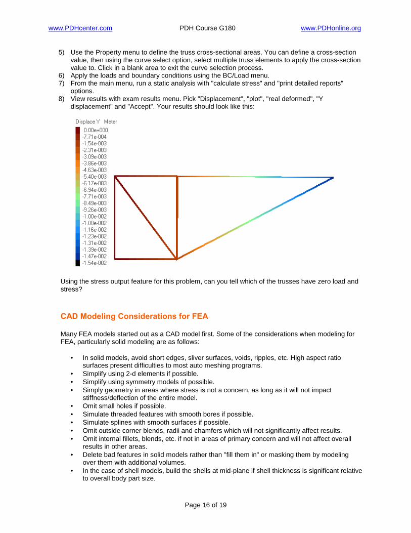
options. 8) View results with exam results menu. Pick "Displacement", "plot", "real deformed", "Y

displacement" and "Accept". Your results should look like this:

Using the stress output feature for this problem, can you tell which of the trusses have zero load and stress? CAD Modeling Considerations for FEA Many FEA models started out as a CAD model first. Some of the considerations when modeling for FEA, particularly solid modeling are as follows:

• In solid models, avoid short edges, sliver surfaces, voids, ripples, etc. High aspect ratio surfaces present difficulties to most auto meshing programs.

• Simplify using 2-d elements if possible. • Simplify using symmetry models of possible. • Simply geometry in areas where stress is not a concern, as long as it will not impact

stiffness/deflection of the entire model. • Omit small holes if possible. • Simulate threaded features with smooth bores if possible. • Simulate splines with smooth surfaces if possible. • Omit outside corner blends, radii and chamfers which will not significantly affect results. • Omit internal fillets, blends, etc. if not in areas of primary concern and will not affect overall

results in other areas. • Delete bad features in solid models rather than "fill them in" or masking them by modeling

over them with additional volumes. • In the case of shell models, build the shells at mid-plane if shell thickness is significant relative

to overall body part size.


Page 17 of 19

• For 2-D line models, check for redundant, or overlapping lines and arcs, unnecessary centerline or center marks, points, etc.

• Use CAD software which is highly compatible with the FEA modeler. • If you are not the CAD designer, consult with CAD designer ahead of time to discuss the FEA

model vs. the actual prototype or production model to discuss how modeling will impact the FEA results.

• Give preference to STEP, ACIS, and Parasolids type model import files and avoid IGES and DXF types if possible.

Von Mises Stress

Von Mises stress results are often used as the output from FEA models, because they represent the complete state of stress at any point of the model numerically. What exactly is the von Mises Stress? It is a calculated value based on distortion energy theory, stating that failure will occur by yielding when the von Mises stress exceeds the yield strength of the material. The von Mises stress is a widely accepted failure criteria for ductile materials, and fits the experimental data well. It is calculated from the three principle stresses as follows:

( ) ( ) ( ) 2/1231

22

23221

−+−+−=

σσσσσσσ vm

Note that since the von Mises stress represents the distortion energy, it will always have a positive sign, even under compressive stress conditions. 3-D Solid Model Example: Pressure Cylinder

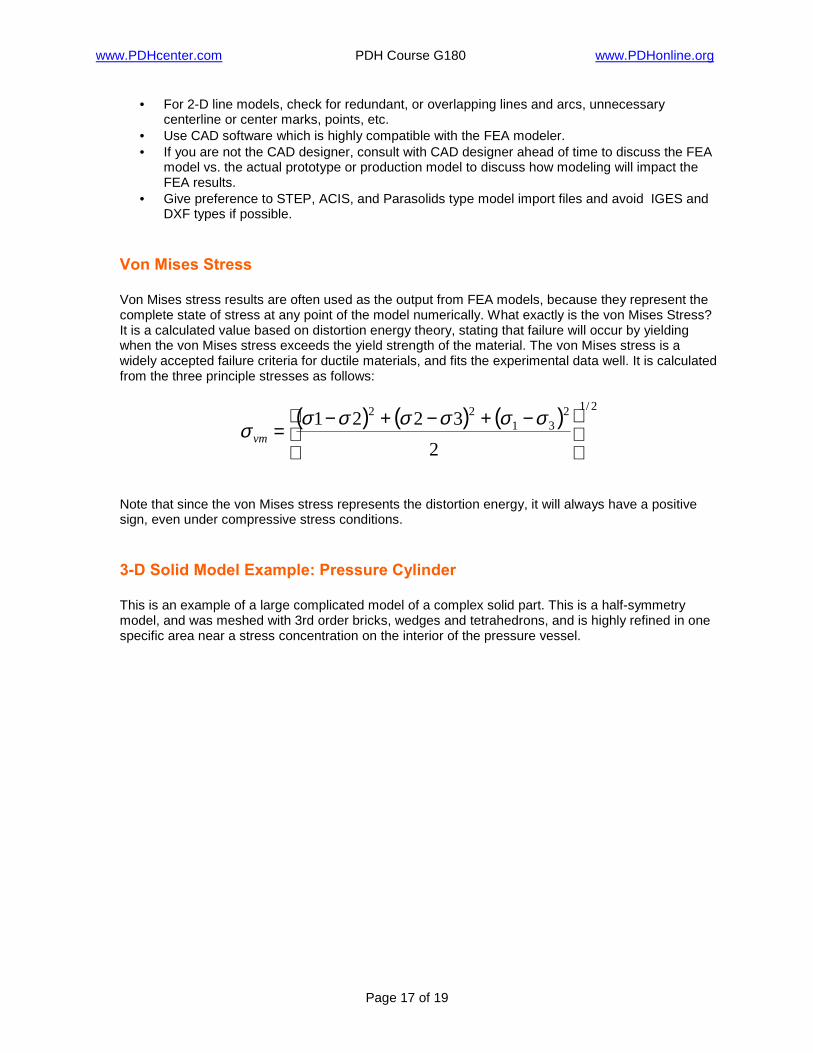
This is an example of a large complicated model of a complex solid part. This is a half-symmetry model, and was meshed with 3rd order bricks, wedges and tetrahedrons, and is highly refined in one specific area near a stress concentration on the interior of the pressure vessel.


Page 18 of 19

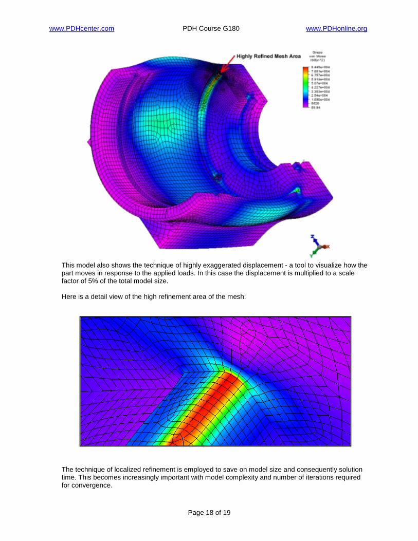
This model also shows the technique of highly exaggerated displacement - a tool to visualize how the part moves in response to the applied loads. In this case the displacement is multiplied to a scale factor of 5% of the total model size. Here is a detail view of the high refinement area of the mesh:

The technique of localized refinement is employed to save on model size and consequently solution time. This becomes increasingly important with model complexity and number of iterations required for convergence.


Page 19 of 19

Summary Linear static FEA is a powerful tool but must be used carefully by analysts with a firm understanding of the physics of the problem, the capabilities and limitations of the FEA code and elements employed, and modeling assumptions. A methodology which includes reality checks, verification of results and mesh convergence iterations will yield the best results. Bibliography Adams V. & Askenazi A. "Building Better Products with Finite Element Analysis." Santa Fe, NM, USA: OnWord Press, 1999. Beer, F. & Johnston, R. "Mechanics of Materials." New York: McGraw-Hill, 1981. Cook, R. "Finite Element Modeling for Stress Analysis." New York: John Wiley & Sons, Inc., 1995. Roark, R. & Young, W. "Formulas for Stress and Strain." New York: McGraw-Hill, 1982. Shigley, J. & Mitchell, L. "Mechanical Engineering Design." New York: McGraw-Hill, 1983

Basic Applied Finite Element Analysis · Plate Element Model of a Thin-Walled Bottle Under Pressure • 3D Solid Element Models: Most commonly used for bulky or chunky parts with

Documents