AutomaticallyEstimatingtheSavingsPotentialof Occupancy ...

Automatically Estimating the Savings Potential of

Occupancy-based Heating Strategies

Vincent Becker∗, Wilhelm Kleiminger, Friedemann Mattern

Institute for Pervasive Computing, Department of Computer Science, ETH Zurich

Abstract

A large fraction of energy consumed in households is due to space heating.

Especially during daytime, the heating is often running constantly, controlled

only by a thermostat – even if the inhabitants are not present. Taking advan-

tage of the absence of the inhabitants to save heating energy by lowering the

temperature thus poses a great opportunity. Since the concrete savings of an

occupancy-based heating strategy strongly depend on the individual occupancy

pattern, a fast and inexpensive method to quantify these potential savings would

be beneficial.

In this paper we present such a practical method which builds upon an ap-

proach to estimate a household’s occupancy from its historical electricity con-

sumption data, as gathered by smart meters. Based on the derived occupancy

data, we automatically calculate the potential savings. Besides occupancy data,

the underlying model also takes into account publicly available weather data

and relevant building characteristics. Using this approach, households with

high potential for energy savings can be quickly identified and their members

could be more easily convinced to adopt an occupancy-based heating strategy

(either by manually adjusting the thermostat or by investing in automation)

since their monetary benefits can be calculated and the risk of misinvestment is

thus reduced.

∗Corresponding authorEmail addresses: [email protected] (Vincent Becker),

[email protected] (Wilhelm Kleiminger), [email protected] (FriedemannMattern)

Submitted for publication December 6, 2017

To prove the usefulness of our system, we apply it to a large dataset con-

taining relevant building and household data such as the size and age of several

thousand households and show that, on average, a household can save over 9%

heating energy when following an occupancy-based heating regime, while certain

groups, such as single-person households, can even save 14% on average.

Keywords: Smart heating, Occupancy detection, Household heating

simulation, Energy savings, Smart energy

1. Introduction

Space heating is the main factor driving the energy consumption of house-

holds. In 2012, heating dominated the consumption of energy of households

in the EU with 67% of total energy use [1]. The residential sector overall ac-

counted for 25% of the final energy consumption in the European Union (EU),5

similar to the industry sector [2]. These numbers are similar for many developed

countries [3]. Due to these large amounts, space heating in households bears

great potential for energy savings, leading to both financial and environmental

benefits. These benefits are growing as energy prices, despite their short-term

volatility, tend to increase over the long run [4, 5]. Several initiatives have been10

taken in recent years to improve the energy efficiency of households. In the EU,

every member state has to regularly create a National Energy Efficiency Action

Plan (NEEAP) according to the Energy Efficiency Directive [6] and must up-

date these plans every three years. In its 2010 plan “Energy 2020 - A strategy

for competitive, sustainable and secure energy” [7], the EU targets overall en-15

ergy savings of 20% by 2020 and in 2016 the European Commission proposed

an update of the Energy Efficiency Directive with a target of 30% by 2030 [8].

One possibility to decrease the amount of heating energy consumed is to

use a heating strategy which is based on the occupancy of the dwelling. The

way most common heating systems still work nowadays is that the user has to20

manually adjust the thermostat to control the temperature. Usually, once the

thermostat has been set, it is left in the same setting as long as the inhabitants

2

feel comfortable with the temperature. The house is thereby heated irrespec-

tively of whether it is occupied or not. In other cases, the thermostat runs on a

fixed schedule that can only coarsely approximate the real occupancy schedule.25

However, when a building is unoccupied, the heating could be turned down in

order to save energy.

This strategy could be carried out in different ways. The inhabitants could

simply take care to turn down the temperature themselves whenever they leave.

Nowadays this is becoming easier with the use of heating systems which can30

be controlled remotely by smartphone apps or the possibility to set a heating

schedule adjusted to one’s own schedule. Additionally, there are heating systems

which are based on automatically detecting the occupancy of a dwelling. These

systems are part of what is known as the smart heating domain [9].

In order to make residents aware of potential savings, a simple, inexpensive,35

and fast method to estimate the savings when applying an occupancy-based

heating strategy would be desirable. Furthermore, households with high poten-

tial should be easily identifiable to promote the installation of an occupancy-

based smart heating system. Although smart heating systems are slowly gaining

more and more interest and are being increasingly used in households [10, 11],40

it might be necessary to convince customers of their benefits and provide a cal-

culation to see whether it is worth the effort and cost of having one installed.

An easily applicable method to estimate the savings of a particular household

with its characteristic occupancy pattern when using a smart heating system

would hence be beneficial. In the following we present such a system which we45

have developed.

2. Approach

Our aim is to estimate the potential heating energy savings for a period in the

past by first learning the occupancy pattern in that period from a household’s

electrical consumption and then simulating its thermal energy consumption op-50

timised to this particular occupancy pattern. The simulation relies on four sets

3

of parameters:

(1) Occupancy. The simulation requires the occupancy schedule, i.e. a timeline

when the home is occupied or unoccupied, which is computed prior to the sim-

ulation. The lower the occupancy, the higher the potential savings, since the55

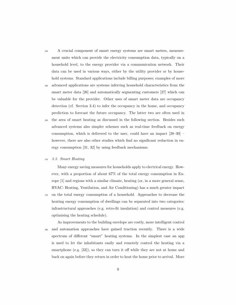
heating could be turned down in times of absence. As an example for the impor-

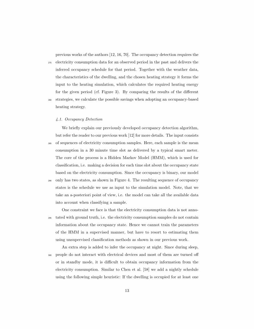
tance of the latter, Figure 1a and Figure 1b show the average weekly occupancy

pattern of two households with distinctively different occupancy schedules. For

the first, the dwelling is occupied most of the time in the early mornings and

evenings. Here, a heating strategy based on occupancy may yield only low sav-60

ings. Conversely, for the second, the dwelling is often unoccupied, even some

nights and the heating could be turned off during these long periods of absence.

Since the savings potential heavily depends on the occupancy, and in particu-

lar on the length and frequency of absence, detecting whether a dwelling was

occupied or not during a given period of time constitutes a crucial part of our65

approach. Previous research [12] has shown that it is possible to detect occu-

pancy automatically with sufficient accuracy from electrical load data (even for

coarse-grained 30 minute measurement intervals) using machine learning algo-

rithms (cf. Section 3.4). Electricity consumption data is indeed a good proxy

for a household’s occupancy since its magnitude and changes over time are indi-70

cators of human activities (i.e. use of appliances) in the household. At the same

time, smart meters, which continuously measure the electrical power consump-

tion of a household, are becoming increasingly ubiquitous [13, 14]: A penetration

rate of 95% is expected in sixteen EU member countries by 2020 [15].

(2) Characteristics of the dwelling. The amount of heating energy used strongly75

depends on the characteristics of the dwelling, such as how well-insulated and

how large it is. For example, to heat an unoccupied dwelling consumes more

energy if the insulation is poor, hence the potential savings are high in such

cases.

4

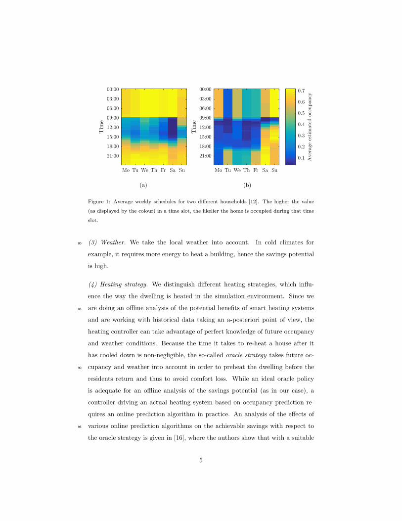
(a) (b)

Figure 1: Average weekly schedules for two different households [12]. The higher the value

(as displayed by the colour) in a time slot, the likelier the home is occupied during that time

slot.

(3) Weather. We take the local weather into account. In cold climates for80

example, it requires more energy to heat a building, hence the savings potential

is high.

(4) Heating strategy. We distinguish different heating strategies, which influ-

ence the way the dwelling is heated in the simulation environment. Since we

are doing an offline analysis of the potential benefits of smart heating systems85

and are working with historical data taking an a-posteriori point of view, the

heating controller can take advantage of perfect knowledge of future occupancy

and weather conditions. Because the time it takes to re-heat a house after it

has cooled down is non-negligible, the so-called oracle strategy takes future oc-

cupancy and weather into account in order to preheat the dwelling before the90

residents return and thus to avoid comfort loss. While an ideal oracle policy

is adequate for an offline analysis of the savings potential (as in our case), a

controller driving an actual heating system based on occupancy prediction re-

quires an online prediction algorithm in practice. An analysis of the effects of

various online prediction algorithms on the achievable savings with respect to95

the oracle strategy is given in [16], where the authors show that with a suitable

5

prediction algorithm the theoretical oracle strategy can be approximated with a

prediction accuracy of over 80% and negligible comfort reduction. Thus a good

approximation of the oracle strategy can indeed be implemented in a real-world

space heating system.100

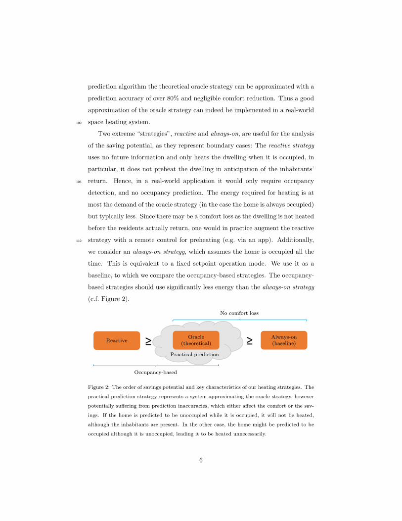
Two extreme “strategies”, reactive and always-on, are useful for the analysis

of the saving potential, as they represent boundary cases: The reactive strategy

uses no future information and only heats the dwelling when it is occupied, in

particular, it does not preheat the dwelling in anticipation of the inhabitants’

return. Hence, in a real-world application it would only require occupancy105

detection, and no occupancy prediction. The energy required for heating is at

most the demand of the oracle strategy (in the case the home is always occupied)

but typically less. Since there may be a comfort loss as the dwelling is not heated

before the residents actually return, one would in practice augment the reactive

strategy with a remote control for preheating (e.g. via an app). Additionally,110

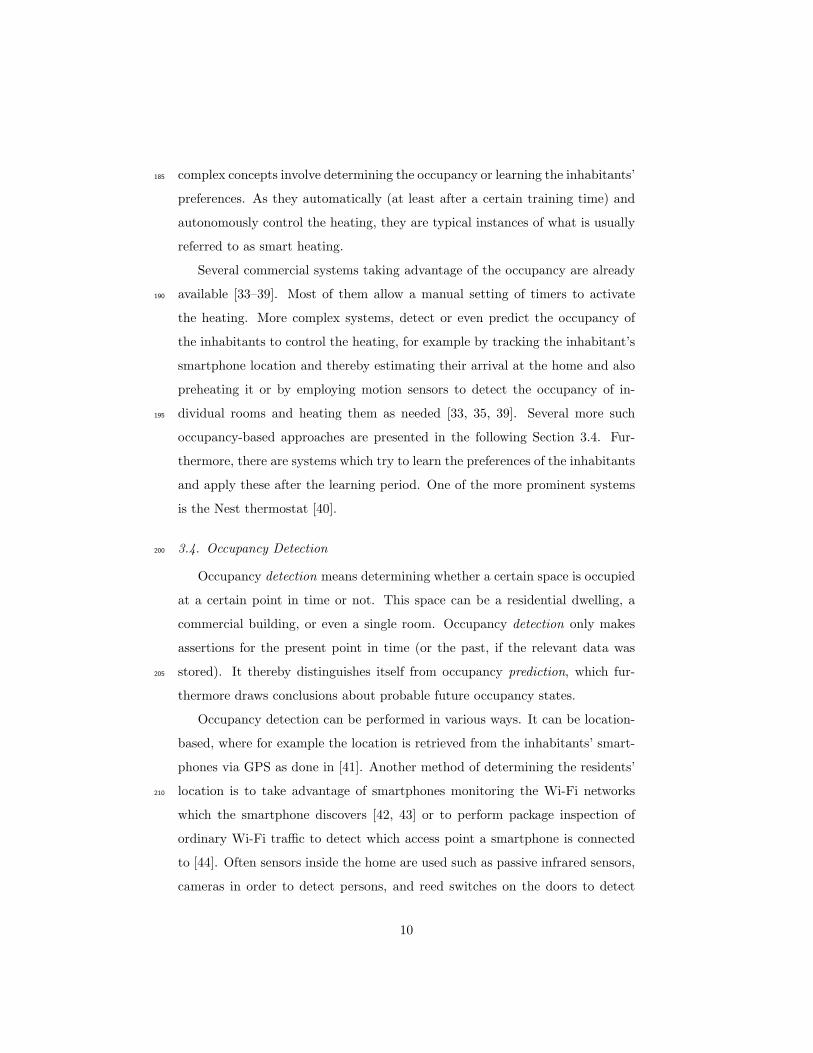
we consider an always-on strategy, which assumes the home is occupied all the

time. This is equivalent to a fixed setpoint operation mode. We use it as a

baseline, to which we compare the occupancy-based strategies. The occupancy-

based strategies should use significantly less energy than the always-on strategy

(c.f. Figure 2).

Practical prediction

Always-on(baseline)

ReactiveOracle

(theoretical)≥

No comfort loss

Occupancy-based

≥

Figure 2: The order of savings potential and key characteristics of our heating strategies. The

practical prediction strategy represents a system approximating the oracle strategy, however

potentially suffering from prediction inaccuracies, which either affect the comfort or the sav-

ings. If the home is predicted to be unoccupied while it is occupied, it will not be heated,

although the inhabitants are present. In the other case, the home might be predicted to be

occupied although it is unoccupied, leading it to be heated unnecessarily.

6

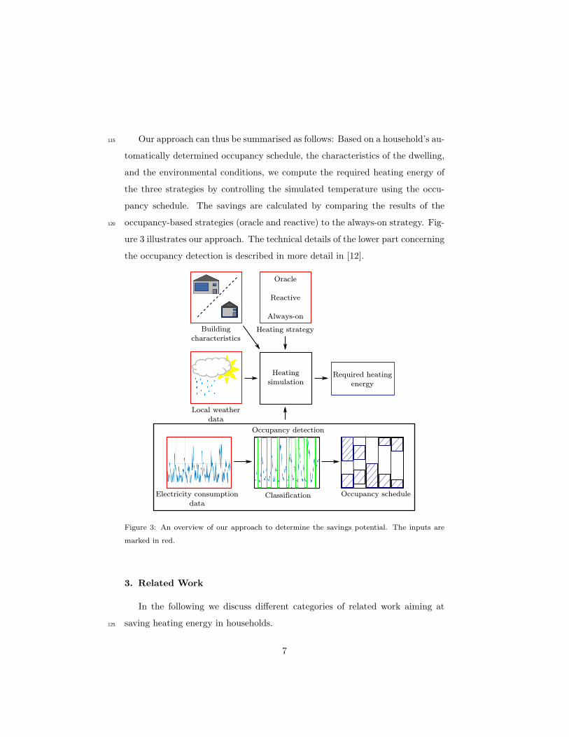
Our approach can thus be summarised as follows: Based on a household’s au-115

tomatically determined occupancy schedule, the characteristics of the dwelling,

and the environmental conditions, we compute the required heating energy of

the three strategies by controlling the simulated temperature using the occu-

pancy schedule. The savings are calculated by comparing the results of the

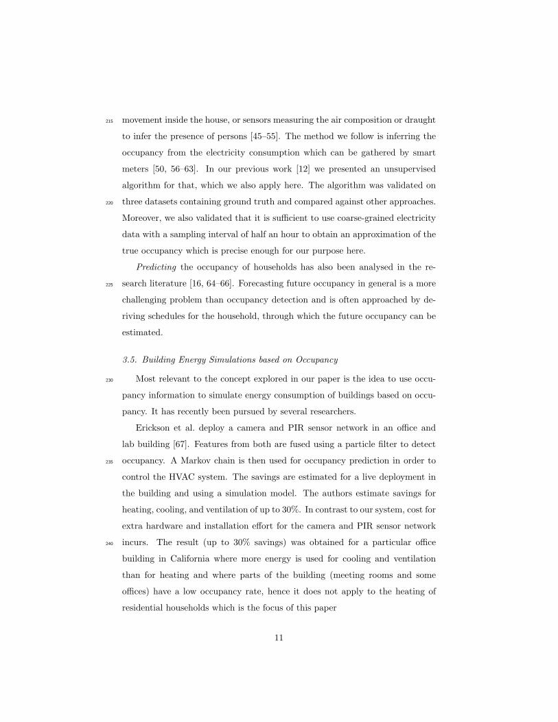
occupancy-based strategies (oracle and reactive) to the always-on strategy. Fig-120

ure 3 illustrates our approach. The technical details of the lower part concerning

the occupancy detection is described in more detail in [12].

Electricity consumption

dataClassification Occupancy schedule

Heating

simulation

Local weather

data

Building

characteristics

Required heating

energy

Heating strategy

Oracle

Reactive

Always-on

Occupancy detection

Figure 3: An overview of our approach to determine the savings potential. The inputs are

marked in red.

3. Related Work

In the following we discuss different categories of related work aiming at

saving heating energy in households.125

7

3.1. Traditional Space Heating Energy Savings Campaigns

The most common efforts to encourage heating energy savings nowadays are

made by institutions, especially on a governmental level, employing campaigns

or incentives to advocate saving energy. One main strategy across many coun-

tries is funding incentives for increasing the energy efficiency of dwellings, either130

in terms of the construction or the heating devices, e.g. the replacement of old

boilers. Examples are energy savings campaigns and grants for energy efficiency

modernisations (e.g. [17–20]), consulting services, either in form of counsel by

experts (e.g. [17, 21, 22]) or brochures and websites (e.g. [17, 23–25]). The ex-

amples demonstrate that a substantial amount of money is invested, especially135

from public institutions, in more fuel-efficient heating systems and building im-

provements.

Our approach is different in two ways. First, we examine savings by reducing

the time the dwelling is heated, not by improving the heating efficiency or

the building (which represent independent, additional saving opportunities). A140

simple form of occupancy-based heating could be applied by the inhabitants

immediately without extra cost, if they took care to turn the heating on and off

themselves. Second, our method allows to identify households with high savings

potential and thereby makes investments (e.g. in smart heating systems) more

efficient and lowers the financial risk thereof.145

3.2. Smart Energy and Consumption Feedback

In recent years there has been a surge in effort invested in the area of so-called

smart energy by both research and industry. This area comprises a variety of

technologies concerning energy generation, storage, transmission, and consump-

tion. It addresses all parts of the value chain from the generation to the use150

of energy, in particular electrical energy. The term “smart” relates to the idea

of using automated and intelligent systems (usually based on advanced infor-

mation and communication technology, such as sensors and data analytics) to

reach the aforementioned goals.

8

A crucial component of smart energy systems are smart meters, measure-155

ment units which can provide the electricity consumption data, typically on a

household level, to the energy provider via a communication network. Their

data can be used in various ways, either by the utility provider or by house-

hold systems. Standard applications include billing purposes; examples of more

advanced applications are systems inferring household characteristics from the160

smart meter data [26] and automatically segmenting customers [27] which can

be valuable for the provider. Other uses of smart meter data are occupancy

detection (cf. Section 3.4) to infer the occupancy in the home, and occupancy

prediction to forecast the future occupancy. The latter two are often used in

the area of smart heating as discussed in the following section. Besides such165

advanced systems also simpler schemes such as real-time feedback on energy

consumption, which is delivered to the user, could have an impact [28–30] –

however, there are also other studies which find no significant reduction in en-

ergy consumption [31, 32] by using feedback mechanisms.

3.3. Smart Heating170

Many energy saving measures for households apply to electrical energy. How-

ever, with a proportion of about 67% of the total energy consumption in Eu-

rope [1] and regions with a similar climate, heating (or, in a more general sense,

HVAC: Heating, Ventilation, and Air Conditioning) has a much greater impact

on the total energy consumption of a household. Approaches to decrease the175

heating energy consumption of dwellings can be separated into two categories:

infrastructural approaches (e.g. retro-fit insulation) and control measures (e.g.

optimising the heating schedule).

As improvements to the building envelope are costly, more intelligent control

and automation approaches have gained traction recently. There is a wide180

spectrum of different “smart” heating systems. In the simplest case an app

is used to let the inhabitants easily and remotely control the heating via a

smartphone (e.g. [33]), so they can turn it off while they are not at home and

back on again before they return in order to heat the home prior to arrival. More

9

complex concepts involve determining the occupancy or learning the inhabitants’185

preferences. As they automatically (at least after a certain training time) and

autonomously control the heating, they are typical instances of what is usually

referred to as smart heating.

Several commercial systems taking advantage of the occupancy are already

available [33–39]. Most of them allow a manual setting of timers to activate190

the heating. More complex systems, detect or even predict the occupancy of

the inhabitants to control the heating, for example by tracking the inhabitant’s

smartphone location and thereby estimating their arrival at the home and also

preheating it or by employing motion sensors to detect the occupancy of in-

dividual rooms and heating them as needed [33, 35, 39]. Several more such195

occupancy-based approaches are presented in the following Section 3.4. Fur-

thermore, there are systems which try to learn the preferences of the inhabitants

and apply these after the learning period. One of the more prominent systems

is the Nest thermostat [40].

3.4. Occupancy Detection200

Occupancy detection means determining whether a certain space is occupied

at a certain point in time or not. This space can be a residential dwelling, a

commercial building, or even a single room. Occupancy detection only makes

assertions for the present point in time (or the past, if the relevant data was

stored). It thereby distinguishes itself from occupancy prediction, which fur-205

thermore draws conclusions about probable future occupancy states.

Occupancy detection can be performed in various ways. It can be location-

based, where for example the location is retrieved from the inhabitants’ smart-

phones via GPS as done in [41]. Another method of determining the residents’

location is to take advantage of smartphones monitoring the Wi-Fi networks210

which the smartphone discovers [42, 43] or to perform package inspection of

ordinary Wi-Fi traffic to detect which access point a smartphone is connected

to [44]. Often sensors inside the home are used such as passive infrared sensors,

cameras in order to detect persons, and reed switches on the doors to detect

10

movement inside the house, or sensors measuring the air composition or draught215

to infer the presence of persons [45–55]. The method we follow is inferring the

occupancy from the electricity consumption which can be gathered by smart

meters [50, 56–63]. In our previous work [12] we presented an unsupervised

algorithm for that, which we also apply here. The algorithm was validated on

three datasets containing ground truth and compared against other approaches.220

Moreover, we also validated that it is sufficient to use coarse-grained electricity

data with a sampling interval of half an hour to obtain an approximation of the

true occupancy which is precise enough for our purpose here.

Predicting the occupancy of households has also been analysed in the re-

search literature [16, 64–66]. Forecasting future occupancy in general is a more225

challenging problem than occupancy detection and is often approached by de-

riving schedules for the household, through which the future occupancy can be

estimated.

3.5. Building Energy Simulations based on Occupancy

Most relevant to the concept explored in our paper is the idea to use occu-230

pancy information to simulate energy consumption of buildings based on occu-

pancy. It has recently been pursued by several researchers.

Erickson et al. deploy a camera and PIR sensor network in an office and

lab building [67]. Features from both are fused using a particle filter to detect

occupancy. A Markov chain is then used for occupancy prediction in order to235

control the HVAC system. The savings are estimated for a live deployment in

the building and using a simulation model. The authors estimate savings for

heating, cooling, and ventilation of up to 30%. In contrast to our system, cost for

extra hardware and installation effort for the camera and PIR sensor network

incurs. The result (up to 30% savings) was obtained for a particular office240

building in California where more energy is used for cooling and ventilation

than for heating and where parts of the building (meeting rooms and some

offices) have a low occupancy rate, hence it does not apply to the heating of

residential households which is the focus of this paper

11

Kim et al. employ linear regression based on electricity use data to estimate245

the number of occupants in a building and use this number to calibrate energy

building models to improve the prediction performance of building energy con-

sumption [68]. Their system is evaluated on data from an office and two campus

buildings. Our approach differs in several ways: we apply our system to resi-

dential households, which have a less regular schedule, use a simulation model250

to predict heating energy consumption, and finally we are able to calculate

potential savings by comparing different heating strategies.

Gluck et al. explore the tradeoffs for a HVAC control system between the pre-

diction performance, energy savings, and comfort loss [69]. They collect ground

truth occupancy data from an office building and simulate an occupancy pre-255

diction algorithm. Random errors of varying number are inserted to evaluate

different prediction performances and their effect on savings and comfort. Ad-

ditionally, the authors compare the predictive strategy to a reactive and a static

strategy and assess different target temperature ranges. The estimated savings

for a predictive in relation to a static strategy are around 10% - 25% for an260

allowed deviation of 6◦C from the setpoint temperature, depending on the error

rates of the occupancy prediction. In comparison, our target domain is resi-

dential households and the dwellings in the dataset we use are spread over an

entire country. We do not require occupancy ground truth, but employ an occu-

pancy estimation algorithm based only on the electricity consumption available265

through smart meters. Furthermore, we use a generic model which requires only

the provision of a few characteristic parameters regarding the dwelling and the

local weather conditions. Thus, our approach is applicable to a large variety of

households very easily and without a great overhead and could directly be used

in a real-world application.270

4. System Design

The crucial concept of our system is the combination of automatic occupancy

detection and heating simulation. Both parts have been explored separately in

12

previous works of the authors [12, 16, 70]. The occupancy detection requires the

electricity consumption data for an observed period in the past and delivers the275

inferred occupancy schedule for that period. Together with the weather data,

the characteristics of the dwelling, and the chosen heating strategy it forms the

input to the heating simulation, which calculates the required heating energy

for the given period (cf. Figure 3). By comparing the results of the different

strategies, we calculate the possible savings when adopting an occupancy-based280

heating strategy.

4.1. Occupancy Detection

We briefly explain our previously developed occupancy detection algorithm,

but refer the reader to our previous work [12] for more details. The input consists

of sequences of electricity consumption samples. Here, each sample is the mean285

consumption in a 30 minute time slot as delivered by a typical smart meter.

The core of the process is a Hidden Markov Model (HMM), which is used for

classification, i.e. making a decision for each time slot about the occupancy state

based on the electricity consumption. Since the occupancy is binary, our model

only has two states, as shown in Figure 4. The resulting sequence of occupancy290

states is the schedule we use as input to the simulation model. Note, that we

take an a-posteriori point of view, i.e. the model can take all the available data

into account when classifying a sample.

One constraint we face is that the electricity consumption data is not anno-

tated with ground truth, i.e. the electricity consumption samples do not contain295

information about the occupancy state. Hence we cannot train the parameters

of the HMM in a supervised manner, but have to resort to estimating them

using unsupervised classification methods as shown in our previous work.

An extra step is added to infer the occupancy at night. Since during sleep,

people do not interact with electrical devices and most of them are turned off300

or in standby mode, it is difficult to obtain occupancy information from the

electricity consumption. Similar to Chen et al. [58] we add a nightly schedule

using the following simple heuristic: If the dwelling is occupied for at least one

13

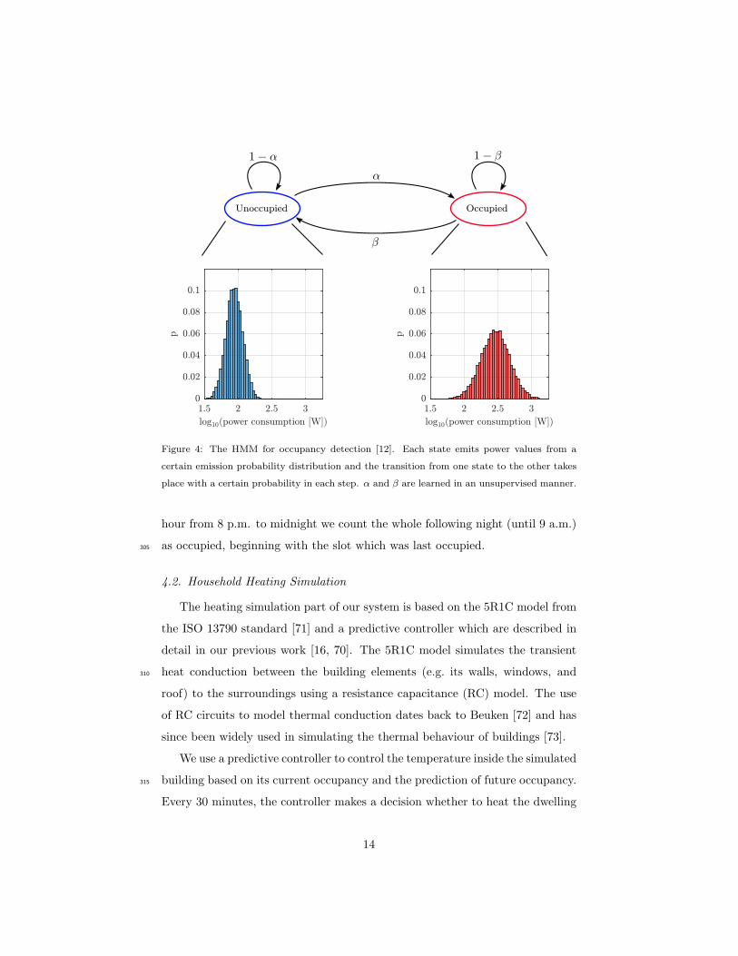
Unoccupied Occupied

Figure 4: The HMM for occupancy detection [12]. Each state emits power values from a

certain emission probability distribution and the transition from one state to the other takes

place with a certain probability in each step. α and β are learned in an unsupervised manner.

hour from 8 p.m. to midnight we count the whole following night (until 9 a.m.)

as occupied, beginning with the slot which was last occupied.305

4.2. Household Heating Simulation

The heating simulation part of our system is based on the 5R1C model from

the ISO 13790 standard [71] and a predictive controller which are described in

detail in our previous work [16, 70]. The 5R1C model simulates the transient

heat conduction between the building elements (e.g. its walls, windows, and310

roof) to the surroundings using a resistance capacitance (RC) model. The use

of RC circuits to model thermal conduction dates back to Beuken [72] and has

since been widely used in simulating the thermal behaviour of buildings [73].

We use a predictive controller to control the temperature inside the simulated

building based on its current occupancy and the prediction of future occupancy.315

Every 30 minutes, the controller makes a decision whether to heat the dwelling

14

or not depending on the heating strategy (cf. Section 2) which is being applied.

For this it takes as input the occupancy, the target temperature, and weather

conditions. The comfort temperature, which should be reached while the house

is occupied, is set to 20◦C (other temperature settings will be discussed in320

Section 6.3). The setback temperature, i.e. the minimum the temperature is

allowed to drop to, is set at 10◦C. The German Federal Environmental Office

advises to set the temperature to 20◦C - 22◦C for the living room, 18◦C for

the kitchen and 17◦C - 18◦C for the bedroom [74]. For periods of absence the

temperature should be reduced to 18◦C, to 15◦C in case of an absence of a325

few days or even lower for longer periods of absence. Hence we think that the

default temperature values we choose for comfort and setback are reasonable.

Note that a setback temperature of 10◦C would only be reached after long

periods of absence in winter, which are rare. For an analysis of the sensitivity

to different temperature settings see Section 6.3.330

As the heating simulation requires the weather data and also building infor-

mation for the particular households, we explain how we obtain this data for

the set of our test households in Section 5.1. Note, however, that our approach

is not specific to households in a certain dataset, but can be applied to any

household for which the necessary parameters are available.335

5. Savings Potential Evaluation

In order to demonstrate our system and gather insights about possible sav-

ing potentials when applying an occupancy-based heating regime, we apply it

to a large dataset containing smart meter data and relevant household char-

acteristics. We use the CER dataset from the Irish Commission for Energy340

Regulation, which is further described in Section 5.1. As the CER dataset

contains no ground truth of the occupancy, we cannot verify the calculated oc-

cupancy values and rely on the algorithms validation carried out in previous

work [12]. After applying our method to each household in the CER dataset

and retrieving the potential savings for each of them, we analyse the savings by345

15

groups, such as singles versus families, since we expect significant differences for

these groups. Furthermore, we examine characteristic properties of households

with higher and lower potential savings, respectively.

5.1. The CER Dataset

The dataset we apply our system to is the CER (Commission for Energy350

Regulation of Ireland) dataset [75]. It contains the power consumption data for

over 4,000 households and small businesses in Ireland. The data we use consists

of 75 weeks’ worth of electricity consumption data measured at intervals of

30 minutes from July 2009 to December 2010. Additionally, the households

participated in a survey in which they had to answer questionnaires in order to355

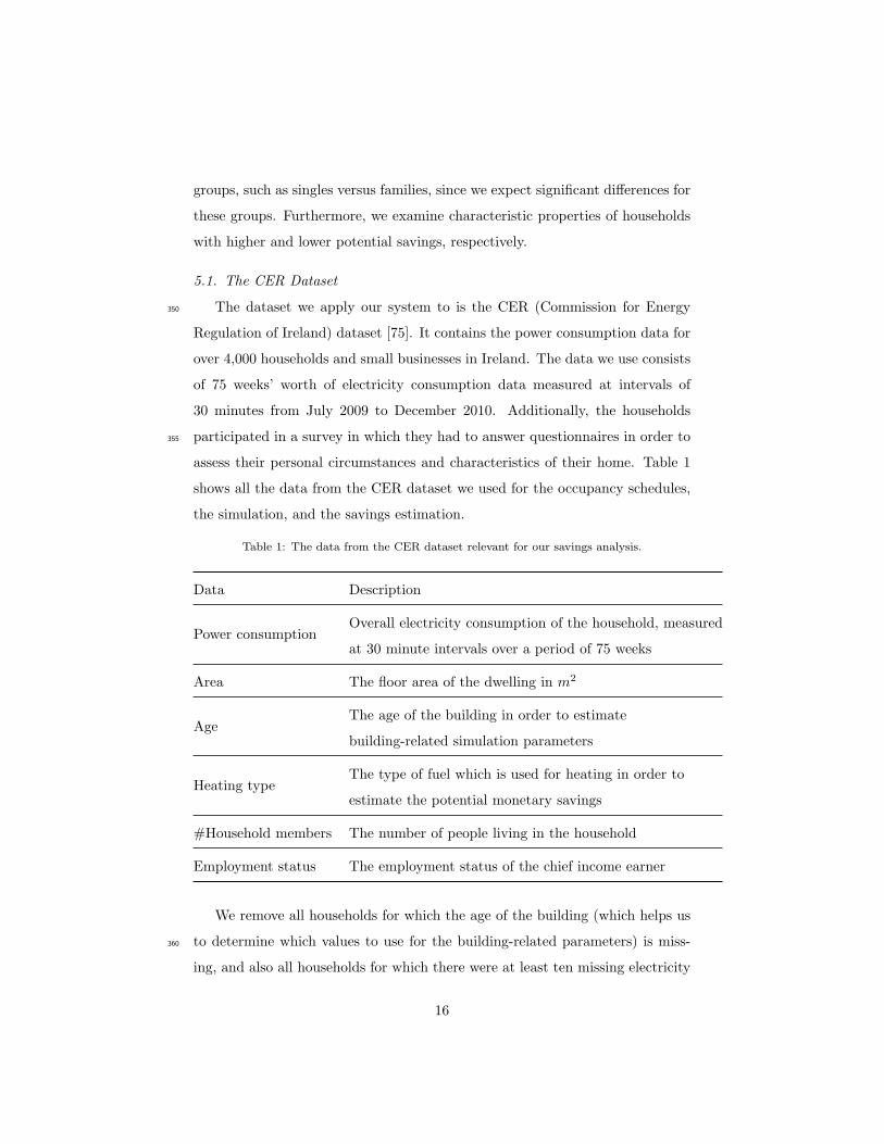
assess their personal circumstances and characteristics of their home. Table 1

shows all the data from the CER dataset we used for the occupancy schedules,

the simulation, and the savings estimation.

Table 1: The data from the CER dataset relevant for our savings analysis.

Data Description

Power consumptionOverall electricity consumption of the household, measured

at 30 minute intervals over a period of 75 weeks

Area The floor area of the dwelling in m2

AgeThe age of the building in order to estimate

building-related simulation parameters

Heating typeThe type of fuel which is used for heating in order to

estimate the potential monetary savings

#Household members The number of people living in the household

Employment status The employment status of the chief income earner

We remove all households for which the age of the building (which helps us

to determine which values to use for the building-related parameters) is miss-360

ing, and also all households for which there were at least ten missing electricity

16

consumption values a day on at least 10 days (e.g. due to smart meter malfunc-

tioning). The final set contains 3,476 households. The data for our analysis

consists only of the electricity load data and the basic information about the

household (c.f. Table 1). A thorough analysis on more household characteristics365

and their classification from electricity data can be found in [76].

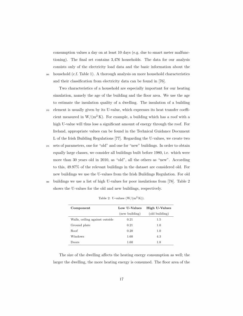
Two characteristics of a household are especially important for our heating

simulation, namely the age of the building and the floor area. We use the age

to estimate the insulation quality of a dwelling. The insulation of a building

element is usually given by its U-value, which expresses its heat transfer coeffi-370

cient measured in W/(m2 K). For example, a building which has a roof with a

high U-value will thus lose a significant amount of energy through the roof. For

Ireland, appropriate values can be found in the Technical Guidance Document

L of the Irish Building Regulations [77]. Regarding the U-values, we create two

sets of parameters, one for “old” and one for “new” buildings. In order to obtain375

equally large classes, we consider all buildings built before 1980, i.e. which were

more than 30 years old in 2010, as “old”, all the others as “new”. According

to this, 49.97% of the relevant buildings in the dataset are considered old. For

new buildings we use the U-values from the Irish Buildings Regulation. For old

buildings we use a list of high U-values for poor insulations from [78]. Table 2380

shows the U-values for the old and new buildings, respectively.

Table 2: U-values (W/(m2 K)).

Component Low U-Values High U-Values

(new building) (old building)

Walls, ceiling against outside 0.21 1.5

Ground plate 0.21 1.0

Roof 0.20 1.0

Windows 1.60 4.3

Doors 1.60 1.8

The size of the dwelling affects the heating energy consumption as well; the

larger the dwelling, the more heating energy is consumed. The floor area of the

17

buildings is derived from the CER dataset. Since we do not know the exact

geometry of the buildings, we assume that they have a square floor space. Each385

of these buildings is given a total window area of 25%, the default value as noted

in the Irish building regulations [77]. As in our previous work, the design heat

load (maximum heating power) of the heating system was determined according

to the European standard EN 12831 [79].

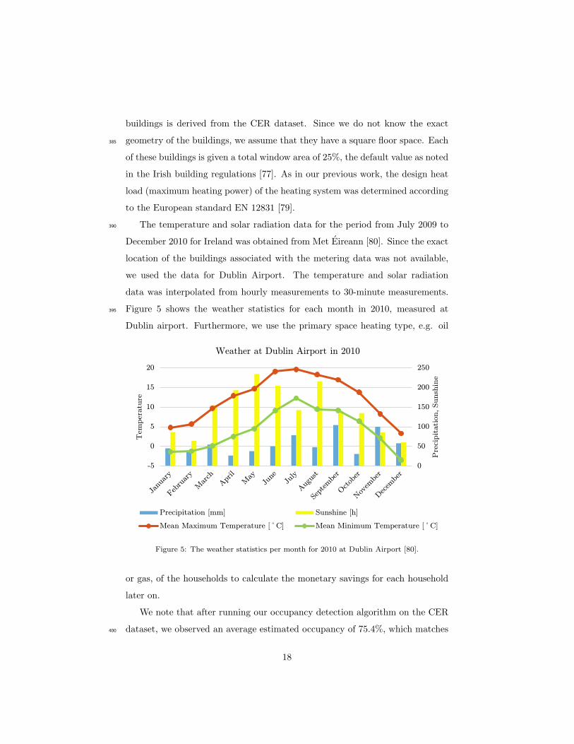
The temperature and solar radiation data for the period from July 2009 to390

December 2010 for Ireland was obtained from Met Eireann [80]. Since the exact

location of the buildings associated with the metering data was not available,

we used the data for Dublin Airport. The temperature and solar radiation

data was interpolated from hourly measurements to 30-minute measurements.

Figure 5 shows the weather statistics for each month in 2010, measured at395

Dublin airport. Furthermore, we use the primary space heating type, e.g. oil

0

50

100

150

200

250

-5

0

5

10

15

20

Pre

cipit

ation, Sunsh

ine

Tem

per

atu

re

Weather at Dublin Airport in 2010

Precipitation [mm] Sunshine [h]

Mean Maximum Temperature [ºC] Mean Minimum Temperature [ºC]

Figure 5: The weather statistics per month for 2010 at Dublin Airport [80].

or gas, of the households to calculate the monetary savings for each household

later on.

We note that after running our occupancy detection algorithm on the CER

dataset, we observed an average estimated occupancy of 75.4%, which matches400

18

the rate of 73.6% reported in the Irish national time use survey [81].

5.2. Savings Calculations

From the heating simulation results we calculate the absolute and relative

savings and also make an estimate on their monetary effects. We calculate the

savings for three different groups: all of the households, those in which the chief405

income earner is employed, and those in which only a single person lives, who

is also employed. The groups vary in the employment and family status. In the

households we examined, 60.3% of the chief income earners were employed or

self-employed (which we count as employed). The reason why these groups are

interesting, is that we expect these characteristics to have a significant influence410

on the occupancy and consequently also on the savings.

As explained in Section 2, the savings we present here are the difference

between the occupancy-based heating strategies, i.e. oracle and reactive on

the one side, and the always-on strategy on the other side. For each of the

occupancy-based strategies and the groups of households we show the mean415

and the sum of absolute, relative, and monetary savings over the full trial time

of 75 weeks. The absolute savings are savings in usable heating energy (i.e. the

output of the heating system and not the input). The fuel energy saved also

depends on the heating system’s efficiency, i.e. how much of the input energy

in form of the heating fuel can be transferred into usable heat, and is higher for420

efficiencies less than 1. Consequently, the monetary savings are calculated as

m = a ∗ c/h, where a are the absolute savings, c the cost in cents per kWh for

the specific type of fuel and h is the efficiency of the heating system. The energy

cost were retrieved from [82] as an average of the second half of 2009 and the

full year of 2010, and the efficiencies from [83]. For the electricity we assume425

no storage heaters were used. For solid fuels we average between standard coal,

peat, and wood pellets. For renewables we use the guaranteed feed-in tariffs

of 15 cent/kWh [84]. For the others we assume the same cost and efficiency

as gas. Note, that the latter three cases only account for a small fraction of

the heating systems in the dataset. The average values over the second half430

19

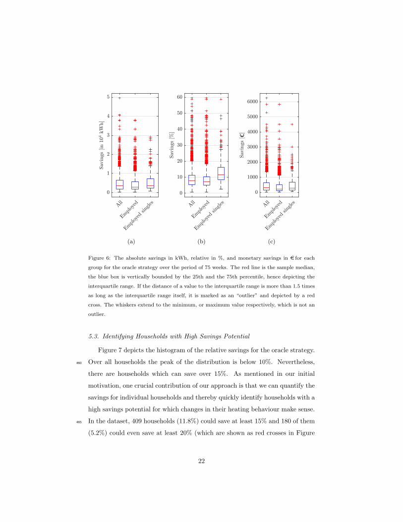
of 2009 and the full year of 2010 for the different types of fuel are shown in

Table 3. The resulting savings are shown in Table 4, Table 5, and in Figure 6.

Table 3: The cost per kWh for the different types of fuel used for space heating and the

estimated efficiency of the corresponding heating systems.

FuelPercentage

in dataset

cent

kWh

Efficiency

old buildings

Efficiency

new buildings

Electricity 6.8% 15.47 1.0 1.0

Gas 30.8% 5.18 0.7 0.9

Oil 55.4% 7.47 0.7 0.9

Solid fuel 6.6% 5.07 0.5 0.74

Renewable 0.2% 15.00 - -

Other 0.2% 5.18 0.7 0.9

Since the results of the oracle and the reactive strategy do not differ much (cf.

Tables 4 and 5) and since the oracle is the more appropriate strategy for a

smart heating system due to the lower comfort loss, we mainly comment on the435

oracle results below, although the main conclusions apply to both strategies and

in particular to possible practical approaches using prediction algorithms [16]

which approximate an oracle occupancy schedule (c.f. Section 2).

A theoretical upper bound of the savings is given by an artificial household,

which is always unoccupied. The savings are the same for the oracle and reactive440

strategy in this case, since the dwelling never has to be heated above the setback

temperature. We simulate two such artificial households, one “new” and one

“old”, with a floor area of 149 m2 (mean in the CER dataset). The relative

savings are 74.16% for the “old” artificial household and 74.82% for the “new”

household. The savings do not amount to 100%, because the heating does have445

to run to uphold the setback temperature.

Over all 3,476 households we observe that on average over 9% energy could

be saved in heating using the oracle strategy (remarkably, this corresponds to the

savings determined for an exemplary scenario in Switzerland in [85], cf. Table 4).

20

Table 4: The average relative savings for each group. n is the number of households in each

group.

Group n Avg. Oracle Avg. Reactive

All 3476 9.24% 10.81%

Employed 2096 8.69% 10.55%

Employed singles 240 13.82% 17.07%

Table 5: The savings for each group over the period of 75 weeks. We show the averages

and sums for each group for absolute and monetary savings. Energy is shown in MWh and

rounded to two decimals or zero decimals for large values, monetary savings are rounded to

the full e.

Group Avg. Oracle∑

Oracle Avg. Reactive∑

Reactive

All4.83 MWh 16,798 MWh 5.48 MWh 19,036 MWh

e465 e1,615,255 e521 e1,811,255

Employed4.24 MWh 8,888 MWh 4.97 MWh 10,408 MWh

e392 e822,393 e453 e950,493

Employed

singles

5.73 MWh 1,376 MWh 6.78 MWh 1,627 MWh

e544 e130,697 e630 e151,245

As we expected, we find the highest savings for the employed singles with nearly450

14% savings, since they are usually at work during daytime and consequently

the home is unoccupied for longer periods of time. These numbers show that

applying occupancy-based strategies could greatly contribute to reaching energy

efficiency goals (cf. Section 1). Moreover, such strategies can create financial

benefits for households. The average savings of e465 over the course of the 75455

weeks are higher than most smart heating systems cost (e.g. Heat Genius [33]

for 249 pounds or the Tado smart thermostat [35] for e199).

21

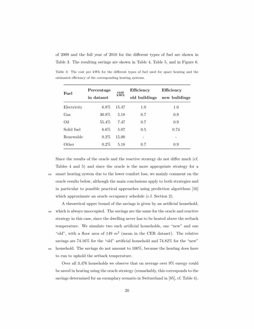
(a) (b)€

(c)

Figure 6: The absolute savings in kWh, relative in %, and monetary savings in e for each

group for the oracle strategy over the period of 75 weeks. The red line is the sample median,

the blue box is vertically bounded by the 25th and the 75th percentile, hence depicting the

interquartile range. If the distance of a value to the interquartile range is more than 1.5 times

as long as the interquartile range itself, it is marked as an “outlier” and depicted by a red

cross. The whiskers extend to the minimum, or maximum value respectively, which is not an

outlier.

5.3. Identifying Households with High Savings Potential

Figure 7 depicts the histogram of the relative savings for the oracle strategy.

Over all households the peak of the distribution is below 10%. Nevertheless,460

there are households which can save over 15%. As mentioned in our initial

motivation, one crucial contribution of our approach is that we can quantify the

savings for individual households and thereby quickly identify households with a

high savings potential for which changes in their heating behaviour make sense.

In the dataset, 409 households (11.8%) could save at least 15% and 180 of them465

(5.2%) could even save at least 20% (which are shown as red crosses in Figure

22

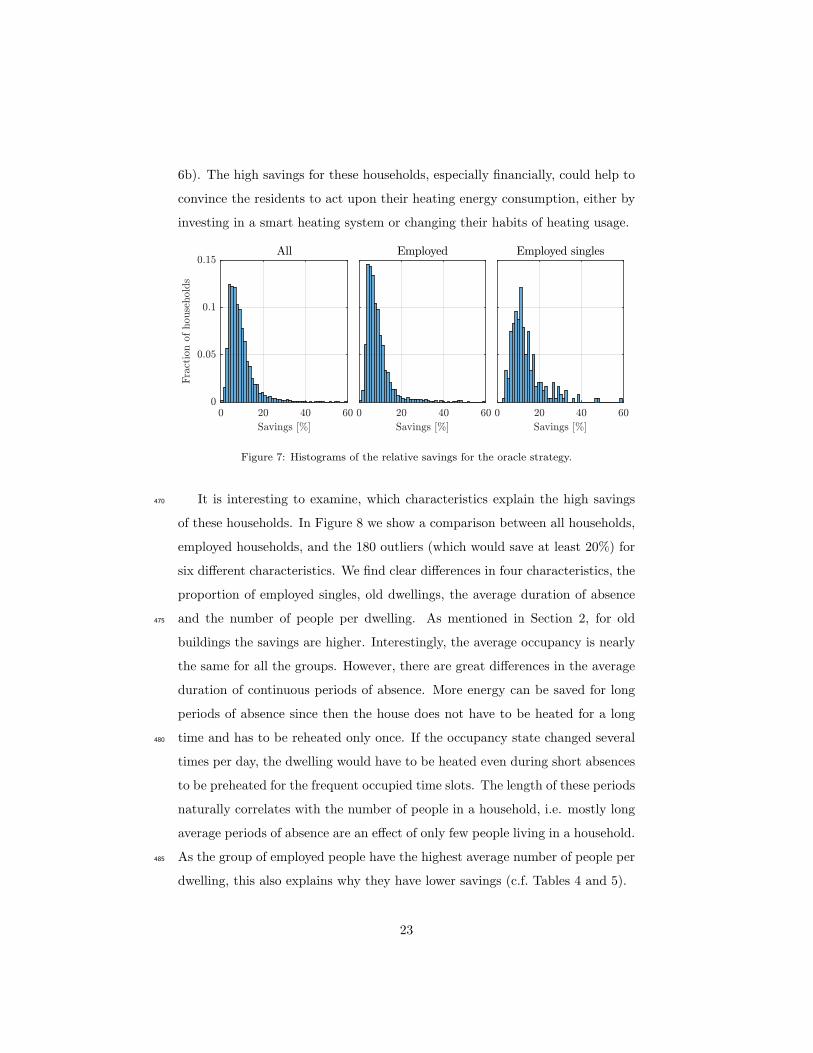
6b). The high savings for these households, especially financially, could help to

convince the residents to act upon their heating energy consumption, either by

investing in a smart heating system or changing their habits of heating usage.

Figure 7: Histograms of the relative savings for the oracle strategy.

It is interesting to examine, which characteristics explain the high savings470

of these households. In Figure 8 we show a comparison between all households,

employed households, and the 180 outliers (which would save at least 20%) for

six different characteristics. We find clear differences in four characteristics, the

proportion of employed singles, old dwellings, the average duration of absence

and the number of people per dwelling. As mentioned in Section 2, for old475

buildings the savings are higher. Interestingly, the average occupancy is nearly

the same for all the groups. However, there are great differences in the average

duration of continuous periods of absence. More energy can be saved for long

periods of absence since then the house does not have to be heated for a long

time and has to be reheated only once. If the occupancy state changed several480

times per day, the dwelling would have to be heated even during short absences

to be preheated for the frequent occupied time slots. The length of these periods

naturally correlates with the number of people in a household, i.e. mostly long

average periods of absence are an effect of only few people living in a household.

As the group of employed people have the highest average number of people per485

dwelling, this also explains why they have lower savings (c.f. Tables 4 and 5).

23

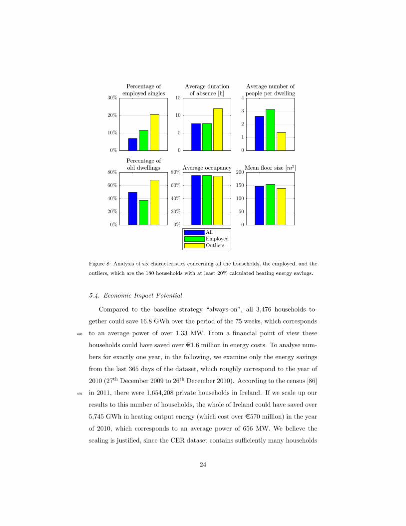
Figure 8: Analysis of six characteristics concerning all the households, the employed, and the

outliers, which are the 180 households with at least 20% calculated heating energy savings.

5.4. Economic Impact Potential

Compared to the baseline strategy “always-on”, all 3,476 households to-

gether could save 16.8 GWh over the period of the 75 weeks, which corresponds

to an average power of over 1.33 MW. From a financial point of view these490

households could have saved over e1.6 million in energy costs. To analyse num-

bers for exactly one year, in the following, we examine only the energy savings

from the last 365 days of the dataset, which roughly correspond to the year of

2010 (27th December 2009 to 26th December 2010). According to the census [86]

in 2011, there were 1,654,208 private households in Ireland. If we scale up our495

results to this number of households, the whole of Ireland could have saved over

5,745 GWh in heating output energy (which cost over e570 million) in the year

of 2010, which corresponds to an average power of 656 MW. We believe the

scaling is justified, since the CER dataset contains sufficiently many households

24

from all over Ireland, and has a similar fuel mix and occupancy rate as the500

whole of the country.

To put the potential energy savings into perspective we compare them to the

total primary energy demand of Ireland in the year of 2010, i.e. all calculations

are done for the period of one year. We scale all numbers to the population of

Ireland. According to [87] the electricity generation efficiency, i.e. the ratio of505

the electricity energy output and the primary energy input for generation, was

46% in 2010. For the households heating with electricity we can calculate their

saved electricity inputs, which results in 497.22 GWh. This means that 1,080.92

GWh primary input for electricity generation could be saved. For all the other

households (excluding those heated with renewables) we calculate their saved510

primary heating input by dividing their saved heating output by the efficiency

of their heating system. These savings in primary energy add up to 7,234.33

GWh. Adding the savings from households heating with electricity, the primary

input savings amount to 8,315.25 GWh. The total primary energy requirement

over all sectors for Ireland is 171,694.44 GWh [88]. In conclusion this means515

that theoretically 4.8% of the primary energy requirement could be saved.

Note that this is only a theoretical potential and may not fully be exploited

for diverse reasons. For example, the baseline (“always-on”) might not be ap-

propriate in all cases as some households might already follow a more disciplined

heating regime. Another reason might be that the occupancy detection and also520

the simulation model (e.g. the estimated U-values of building elements) might be

imprecise. And finally, in some cases the humans’ behavioural reaction to saving

heating cost might be to increase the thermostat setting, thereby diminishing

the savings effect. Some of these issues are further discussed in Section 6.

6. Discussion525

We now discuss and justify some of our assumptions and analyse the stability

and robustness of our method and results.

25

6.1. Nightly Setback

Often, households have a timer-driven heating system which lets the tem-

perature drop to a certain setback temperature at night in order to save energy.530

One could argue that for our analysis a baseline in which the temperature is

decreased during the night makes more sense than the always-on baseline. How-

ever, if we used a baseline with a night-time setback temperature, we could also

use this setback in our occupancy-based strategies, which then consequently

would use even less energy (because at night a home is typically occupied). For535

this setting the savings are even higher (6.64 MWh on average for the oracle

strategy compared to 4.83 MWh over the 75 weeks period). This is due to the

possibility of obtaining schedules with very long periods of absence, e.g. when

the dwelling is unoccupied the whole day, it does not have to be heated above

the setback temperature for the previous night and that day. This effect is540

naturally even stronger for reactive schedules (8.41 MWh instead of 5.48 MWh

energy savings).

6.2. Sensitivity the Occupancy Estimation

As we perform a post-analysis of a household’s energy consumption, em-

ploying occupancy detection is sufficient for our calculations. In a real-world545

setting, this also applies to the reactive strategy, as no future occupancy infor-

mation is needed. However, to be able to employ the oracle strategy in practice,

occupancy prediction is required, which is a more challenging problem. For

neither of the estimation paradigms the corresponding approaches are perfect.

Prediction algorithms additionally face the fact that humans sometimes behave550

inconsistently and not “according to plan”, e.g. spontaneously deciding to skip

their weekly sports training. Research has shown that detection and prediction

can be performed with reasonably high accuracy (e.g. for detection: on average

83% [12], 82% [59], 73% [58], e.g. for prediction 85% [16]). Other systems not

based on electricity consumption, such as Tado [35], which uses the location of555

the inhabitant’s smartphone from which the return time can be estimated, may

even be more accurate (but they require the “augmentation” of the human).

26

Errors in the detection or prediction may impair the savings potential when

the false positive rate is high, i.e. the dwelling is heated when nobody is at

home. The comfort may suffer from the same cause, but from contrary errors,560

false-negatives, i.e. the dwelling is not heated or the temperature is not yet high

enough when the home is in fact occupied. However, in a real-world deployment

there are several possibilities for technical measures to counteract this comfort

loss, e.g. an “override” button inside the home or a smartphone app to overrule

the automatic heating control. The discussion of these means is out of the scope565

of this paper.

As our simulation and as such our savings estimation depend on the out-

put of the occupancy detection, we might be facing second order errors in the

savings estimation due to errors in the occupancy detection. Since we have no

occupancy ground truth for the CER dataset, we cannot directly validate our570

occupancy detection results. We acknowledge that potentially there are errors

in the detection, but the question is how strongly the savings results react to

errors in the occupancy detection, i.e. if the detection makes only a few more

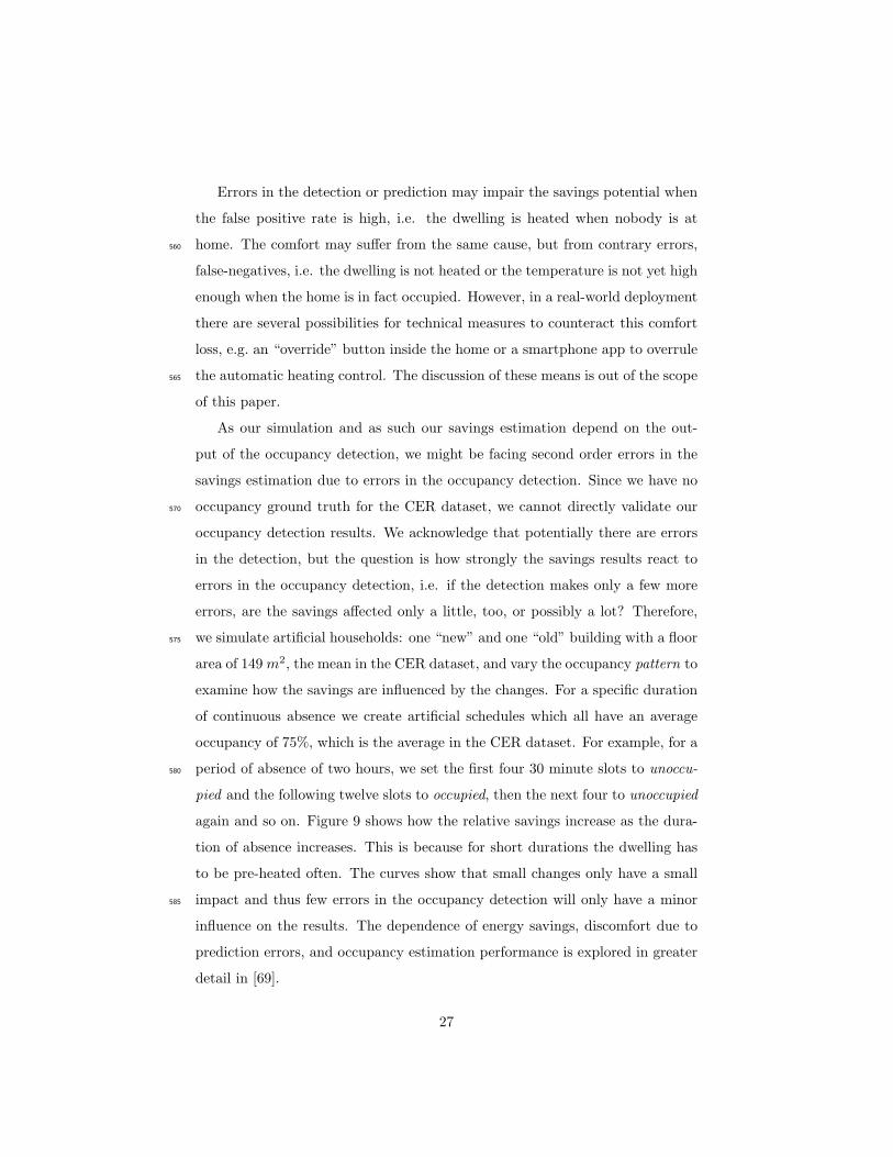
errors, are the savings affected only a little, too, or possibly a lot? Therefore,

we simulate artificial households: one “new” and one “old” building with a floor575

area of 149m2, the mean in the CER dataset, and vary the occupancy pattern to

examine how the savings are influenced by the changes. For a specific duration

of continuous absence we create artificial schedules which all have an average

occupancy of 75%, which is the average in the CER dataset. For example, for a

period of absence of two hours, we set the first four 30 minute slots to unoccu-580

pied and the following twelve slots to occupied, then the next four to unoccupied

again and so on. Figure 9 shows how the relative savings increase as the dura-

tion of absence increases. This is because for short durations the dwelling has

to be pre-heated often. The curves show that small changes only have a small

impact and thus few errors in the occupancy detection will only have a minor585

influence on the results. The dependence of energy savings, discomfort due to

prediction errors, and occupancy estimation performance is explored in greater

detail in [69].

27

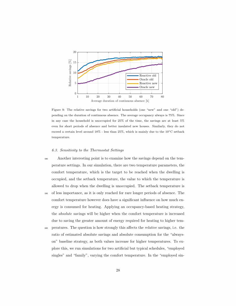
Figure 9: The relative savings for two artificial households (one “new” and one “old”) de-

pending on the duration of continuous absence. The average occupancy always is 75%. Since

in any case the household is unoccupied for 25% of the time, the savings are at least 5%

even for short periods of absence and better insulated new houses. Similarly, they do not

exceed a certain level around 18% - less than 25%, which is mainly due to the 10◦C setback

temperature.

6.3. Sensitivity to the Thermostat Settings

Another interesting point is to examine how the savings depend on the tem-590

perature settings. In our simulation, there are two temperature parameters, the

comfort temperature, which is the target to be reached when the dwelling is

occupied, and the setback temperature, the value to which the temperature is

allowed to drop when the dwelling is unoccupied. The setback temperature is

of less importance, as it is only reached for rare longer periods of absence. The595

comfort temperature however does have a significant influence on how much en-

ergy is consumed for heating. Applying an occupancy-based heating strategy,

the absolute savings will be higher when the comfort temperature is increased

due to saving the greater amount of energy required for heating to higher tem-

peratures. The question is how strongly this affects the relative savings, i.e. the600

ratio of estimated absolute savings and absolute consumption for the “always-

on” baseline strategy, as both values increase for higher temperatures. To ex-

plore this, we run simulations for two artificial but typical schedules, “employed

singles” and “family”, varying the comfort temperature. In the “employed sin-

28

Figure 10: The relative savings for four types of artificial households (typical schedules for

employed singles (ES) and family (F), each of them in a “new” and “old” dwelling) depend-

ing on the comfort temperature setting. The vertical dashed line corresponds to a comfort

temperature of 20◦C, at which we carried out the main evaluation. The red circles mark the

results of repeated simulations for all households in the CER dataset at comfort temperature

settings of 18◦C, 20◦C, and 25◦C using the oracle strategy.

gles” schedule, the dwelling is unoccupied from 9 a.m. to 6 p.m. from Monday605

to Friday, and from 8 p.m. to 11 p.m. on Fridays and Saturdays. In the “family”

schedule, the dwelling is unoccupied from 9 a.m. to 2 p.m. Monday to Friday.

Additionally, for each schedule we simulate a “new” and an “old” dwelling, i.e.

we obtain four artificial households. The comfort temperature is varied from

18◦C to 25◦C in steps of a quarter of a degree. The range corresponds to advice610

on temperature settings for households given by the German Federal Environ-

mental Office [74]. The results are depicted in Figure 10. It shows that the

relative savings only slightly increase when increasing the comfort temperature.

This effect is strongest for the “employed singles” setting with an “old” dwelling

and employing the reactive strategy – however the increase is still less than two615

percent points over the full range. For the “family” setting the relative savings

are nearly constant. We also simulate a third schedule with a daily absence

29

from 2 p.m. to 4 p.m. not shown in the figure, for which the results were also

constant. As usual, the savings are less for the oracle strategy than for the re-

active strategy, but also the increase in savings is less. This is due to a contrary620

effect for the oracle strategy: the higher the comfort temperature, the earlier

the household has to be preheated in periods of absence.

Additionally, we run the simulation for the whole dataset again twice for

the extremes of the examined comfort temperature range, which are marked

as red circles in Figure 10. The average relative savings for all households at625

a comfort temperature of 18◦C were 8.69% and at a comfort temperature of

25◦C 9.94%. The values show little deviation from average relative savings

at a comfort temperature of 20◦C (9.24%, c.f. Table 4), which we used for

evaluation. Overall we find that our relative savings results for the chosen

comfort temperature of 20◦C are also valid for other reasonable temperature630

settings.

6.4. Sensitivity to the Heating Power

In our analysis, we determined the maximum power the heating system of

a dwelling is able to deliver (the so-called design heat load) according to the

European standard EN 12831. One can expect, however, that in practice a635

particular heating system deviates in one way or the other from that standard.

For occupancy-based heating regimes, the available heating power is indeed an

important aspect to consider. The higher it is, the shorter the period a dwelling

has to be preheated before the arrival of the inhabitants when employing the

oracle strategy. Therefore, we expect the savings to be higher with a more640

powerful heating system. For the reactive strategy the opposite is the case. The

reactive strategy only heats the dwelling upon arrival, however then it will try to

heat it up as quickly as possible with all the heating power available, if necessary,

as its primary concern is to minimise the comfort loss of the inhabitants. That

means, with a higher heating power, the comfort will be higher, but also the645

amount of energy consumed.

To examine this matter, we perform similar simulations as in Section 6.3,

30

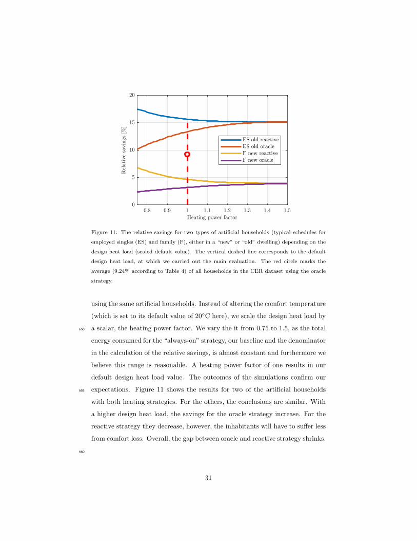
Figure 11: The relative savings for two types of artificial households (typical schedules for

employed singles (ES) and family (F), either in a “new” or “old” dwelling) depending on the

design heat load (scaled default value). The vertical dashed line corresponds to the default

design heat load, at which we carried out the main evaluation. The red circle marks the

average (9.24% according to Table 4) of all households in the CER dataset using the oracle

strategy.

using the same artificial households. Instead of altering the comfort temperature

(which is set to its default value of 20◦C here), we scale the design heat load by

a scalar, the heating power factor. We vary the it from 0.75 to 1.5, as the total650

energy consumed for the “always-on” strategy, our baseline and the denominator

in the calculation of the relative savings, is almost constant and furthermore we

believe this range is reasonable. A heating power factor of one results in our

default design heat load value. The outcomes of the simulations confirm our

expectations. Figure 11 shows the results for two of the artificial households655

with both heating strategies. For the others, the conclusions are similar. With

a higher design heat load, the savings for the oracle strategy increase. For the

reactive strategy they decrease, however, the inhabitants will have to suffer less

from comfort loss. Overall, the gap between oracle and reactive strategy shrinks.

660

31

6.5. Behavioural and Economic Effects

The savings potential discussed in Section 5.4 will not be fully exploited in

practice because of some known adverse effects. For example, the acceptance of

“smart” technology is never at 100%, and some inhabitants would not be willing

to accept an even moderately reduced comfort resulting from prediction errors,665

or they might suspect discomfort for their cherished pets left behind alone at

home. Furthermore, the inhabitants’ anticipation of energy savings may lead

to an adverse behavioural response due to the rebound effect, a known problem

in energy economics [89, 90]. Instead of saving energy and costs by running

their households with the same devices and temperature settings, but with an670

occupancy-based strategy, people may see the potential energy savings as a

reason to increase the temperature in their dwelling, or to buy newer or larger

devices. Thereby the energy consumption is either levelled or even increased.

Furthermore, saving energy in one’s household may lead people to believe they

have reached the moral high ground in terms of energy savings and relieve675

their conscience with regard to energy conservation in other areas of their daily

life, e.g. when driving an energy-inefficient car - a behaviour known as moral

licencing [91, 92]. Such behavioural and economic effects and their impact on

the effective energy savings are important but difficult to estimate, and their

analysis is beyond the scope of this paper.680

6.6. A “Future-Proof Issue”?

Will the saving of energy for space heating still be a relevant issue in the

medium- to long-term future? After all, steady efficiency improvements with

building envelope technologies (better insulation, lower U-Values, etc.), but also

global warming should gradually reduce the problem. In fact, Connolly conjec-685

tures that due to technical improvements to be expected in the coming decades,

heat demand in the EU buildings sector could eventually be halfed [93]. Addi-

tional savings beyond that, however, would be uneconomical, he believes.

While 50% of today’s energy demand is still a relevant share, two other fac-

tors should also be considered. Firstly, the comfort level of indoor temperature690

32

is on the rise, driving up demand for space heating energy. In the UK, for exam-

ple, average indoor temperatures have risen steadily over the past 40 years, from

13◦C in the late 1970ies to around 17.5◦C now (c.f. [94], Table 3.16). Johnston

et al. assume that if the standard of living continues to rise, the mean internal

temperature of UK dwellings will saturate at around 21◦C by 2040 or 2050 [95].695

Secondly, while today households in the EU use on average less than 1%

of their energy for cooling [1], and a lot of building space in Europe is not

cooled at all, Werner notes that for an ideal indoor climate many buildings

should indeed be cooled [96]. The general consensus is that cooling needs will

increase as comfort levels improve in the coming decades. To meet all the700

cooling needs, Werner expects a six-fold increase in the cooling demands in

the EU compared to today. And while global warming by 1 to 2◦C over the

next decades might reduce somewhat the demand for heating energy, it would

conversely drive up electricity demand for cooling purposes. It should be clear

that the technologies for occupancy-based space heating presented in this paper705

can in principle also be used in occupancy-based cooling schemes (or HVAC

control system in general) to save energy and cost [69]. Aftab et al. recently

proposed an occupancy-based HVAC control system to save energy when cooling

mosques [97]. One can expect that this aspect will become more and more

relevant also to many developing countries in the world.710

7. Conclusions

The aim in this work was to provide a method to estimate how much heat-

ing energy one could save by employing an occupancy-based heating strategy

in a private household. We derive occupancy patterns from unlabelled electric-

ity consumption data by applying an unsupervised classification algorithm to715

generate an occupancy schedule. We use this schedule together with basic char-

acteristics of the dwelling (such as its age and its size), and the local weather

data to simulate the heating process in the households and to determine how

much energy could be saved if an occupancy-based heating strategy was applied.

33

If households have a smart metering system and provide the few basic parame-720

ters about their dwelling, our approach could be used to individually estimate

the usefulness of a smart heating system or to teach the inhabitants to what

extent it may be beneficial to change their habits of heating usage. Moreover,

our approach could also be used to assess investments in building improvements,

by varying the characteristic parameters in the simulation. The algorithms we725

presented require little computational power and can easily be run locally in the

home, so there would be no need to disclose occupancy or other data and thus

privacy concerns could be avoided.

We applied our system to the CER dataset, consisting of data of several

thousand households in Ireland. Our results indicate that on average over 9%730

heating energy can theoretically be saved, which would result in significant

monetary and ecological benefits.

8. Acknowledgments

We would like to thank the Irish Social Science Data Archive [98] for the

access to and the permission to work with the CER dataset.735

34

[1] B. Lapillonne, K. Pollier, N. Samci, Energy efficiency trends for households

in the EU, Tech. Rep., ODYSEE-MURE project (2015).

URL http://www.odyssee-mure.eu/publications/efficiency-by-

sector/household/household-eu.pdf

[2] Eurostat, Final energy consumption in the EU [cited 18.05.2017].740

URL http://ec.europa.eu/eurostat/tgm/table.do?tab=

table&plugin=1&language=en&pcode=tsdpc320

[3] Int. Energy Agency, Final energy consumption 2015 [cited 03.12.2017].

URL http://www.iea.org/Sankey/#?c=OECD%20Total&s=Final%

20consumption745

[4] Eurostat, Gas prices in the EU [cited 18.05.2017].

URL http://ec.europa.eu/eurostat/tgm/table.do?tab=table&init=

1&language=en&pcode=ten00118&plugin=1

[5] Eurostat, Electricity prices in the EU [cited 18.05.2017].

URL http://ec.europa.eu/eurostat/statistics-explained/750

index.php/Electricity_price_statistics

[6] European Commission, Energy efficiency directive (2012) [cited 18.05.2017].

URL https://ec.europa.eu/energy/en/topics/energy-efficiency/

energy-efficiency-directive

[7] European Commission, Energy 2020. A strategy for competitive, sustain-755

able and secure energy (2010). doi:10.2833/78930.

[8] European Commission, The new energy efficiency measures (2016) [cited

18.05.2017].

URL https://ec.europa.eu/energy/sites/ener/files/documents/

technical_memo_energyefficiency.pdf760

[9] W. Kleiminger, Occupancy sensing and prediction for automated en-

ergy savings, Ph.D. thesis, ETH Zurich (2015). doi:10.3929/ethz-a-

010450096.

35

[10] IHS Markit, Smart and connected thermostats both provide different

opportunities for manufacturers [cited 31.05.2017].765

URL https://technology.ihs.com/549449/smart-and-connected-

thermostats-both-provide-different-opportunities-for-

manufacturers

[11] Energetics Incorporated, Overview of existing and future residential use

cases for connected thermostats, Tech. Rep., U.S. Department of Energy,770

Washington, DC (2016).

URL https://energy.gov/eere/buildings/downloads/overview-

existing-and-future-residential-use-cases-connected-

thermostats

[12] V. Becker, W. Kleiminger, Exploring zero-training algorithms for occu-775

pancy detection based on smart meter measurements, in: Computer Sci-

ence - Research and Development, 2017, pp. 1–12. doi:10.1007/s00450-

017-0344-9.

[13] U.S. Energy Information Administration, Advanced metering count by

technology type [cited 18.05.2017].780

URL http://www.eia.gov/electricity/annual/html/epa_10_10.html

[14] European Commission, Benchmarking smart metering deployment in the

EU-27 with a focus on electricity, Tech. Rep. 52014DC0356, Brussels

(2014).

URL http://eur-lex.europa.eu/legal-content/EN/TXT/?qid=785

1499933619394&uri=CELEX:52014DC0356

[15] European Commission, Cost-benefit analyses & state of play of smart me-

tering deployment in the EU-27, Tech. Rep. 52014SC0189, Brussels (2014).

URL http://eur-lex.europa.eu/legal-content/EN/TXT/?uri=celex%

3A52014SC0189790

[16] W. Kleiminger, F. Mattern, S. Santini, Predicting household occupancy for

36

smart heating control: A comparative performance analysis of state-of-the-

art approaches, Energy and Buildings 85 (2014) 493–505. doi:10.1016/

j.enbuild.2014.09.046.

[17] Kanton Zurich Baudirektion, Energieforderung Kanton Zurich [cited795

18.05.2017].

URL http://www.energiefoerderung.zh.ch

[18] Sustainable Energy Authority of Ireland, Better energy homes scheme [cited

18.05.2017].

URL http://www.seai.ie/Grants/Better_energy_homes/800

[19] Sustainable Energy Authority of Ireland, Warmer homes scheme [cited

18.05.2017].

URL http://www.seai.ie/Grants/Warmer_Homes_Scheme/

[20] Kreditanstalt fur Wiederaufbau, Energieeffizient Sanieren – Investitions-

zuschuss [cited 01.06.2017].805

URL https://www.kfw.de/inlandsfoerderung/Privatpersonen/

Bestandsimmobilien/Finanzierungsangebote/Energieeffizient-

Sanieren-Zuschuss-(430)/

[21] Verbraucherzentrale Bundesverband e.V., Verbraucherzentrale Energiebe-

ratung [cited 18.05.2017].810

URL https://www.verbraucherzentrale-energieberatung.de/

[22] Bundesamt fur Wirtschaft und Ausfuhrkontrolle, Energieberatung [cited

01.06.2017].

URL http://www.bafa.de/DE/Energie/Energieberatung/Vor_Ort_

Beratung/Beratene/beratene_node.html815

[23] Sustainable Energy Authority of Ireland, SEAI homepage [cited

18.05.2017].

URL www.seai.ie

37

[24] Elektrizitatswerke Kanton Zurich, Energie-Experten [cited 18.05.2017].

URL https://www.energie-experten.ch/de/820

[25] German Federal Government for Environment, Nature Conversation,

Building and Nuclear Safety, Stromsparinitiative [cited 18.05.2017].

URL http://www.die-stromsparinitiative.de/

[26] C. Beckel, L. Sadamori, T. Staake, S. Santini, Revealing household charac-

teristics from smart meter data, Energy 78 (October 2014) (2014) 397–410.825

doi:10.1016/j.energy.2014.10.025.

[27] C. Beckel, L. Sadamori, S. Santini, T. Staake, Automated customer seg-

mentation based on smart meter data with temperature and daylight

sensitivity, in: Proc. IEEE Int. Conf. on Smart Grid Communications,

SmartGridComm, Miami, FL, USA, 2015, pp. 653–658. doi:10.1109/830

SmartGridComm.2015.7436375.

[28] S. Darby, The effectiveness of feedback on energy consumption, A Review

for DEFRA of the Literature on Metering, Billing and direct Displays

486 (2006).

URL http://www.usclcorp.com/news/DEFRA-report-with-835

appendix.pdf

[29] F. Mattern, T. Staake, M. Weiss, ICT for green: how computers can help us

to conserve energy, in: Proc. 1st Int. Conf. on Energy-Efficient Computing

and Networking, e-Energy, Passau, Germany, 2010, pp. 1–10. doi:10.1145/

1791314.1791316.840

[30] M. Weiss, C. Loock, T. Staake, F. Mattern, E. Fleisch, Evaluating mobile

phones as energy consumption feedback devices, in: Mobile and Ubiquitous

Systems: Computing, Networking, and Services - 7th Int. ICST Conf., Mo-

biQuitous 2010, Sydney, Australia, December 6-9, 2010, Revised Selected

Papers, 2010, pp. 63–77. doi:10.1007/978-3-642-29154-8_6.845

38

[31] L. Pereira, F. Quintal, M. Barreto, N. J. Nunes, Understanding the Lim-

itations of Eco-feedback: A One-Year Long-Term Study, Springer Berlin

Heidelberg, 2013, pp. 237–255. doi:10.1007/978-3-642-39146-0_21.

[32] D. Allen, K. Janda, The effects of household characteristics and energy

use consciousness on the effectiveness of real-time energy use feedback: A850

pilot study, in: ACEEE Summer Study on Energy Efficiency in Buildings,

2006.

URL https://www.researchgate.net/publication/281392249_

The_effects_of_household_characteristics_and_energy_use_

consciousness_on_the_effectiveness_of_real-time_energy_use_855

feedback_A_pilot_study

[33] Heat Genius Ltd, Heat genius products [cited 18.05.2017].

URL https://www.geniushub.co.uk/

[34] Honeywell thermostats [cited 18.05.2017].

URL http://getconnected.honeywell.com/de/860

[35] Tado, The smart thermostat [cited 18.05.2017].

URL https://www.tado.com/mt/

[36] British Gas, Hive active heating [cited 18.05.2017].

URL https://www.britishgas.co.uk/products-and-services/hive-

active-heating.html865

[37] Climote, Remote heating control [cited 18.05.2017].

URL http://www.climote.ie/

[38] Starck, Netatmo [cited 18.05.2017].

URL https://www.netatmo.com

[39] Heatmiser, Neo [cited 18.05.2017].870

URL http://www.heatmiser.de/

39

[40] Nest, Nest learning thermostat [cited 18.05.2017].

URL https://nest.com/

[41] M. Gupta, S. S. Intille, K. Larson, Adding GPS-control to traditional ther-

mostats: An exploration of potential energy savings and design challenges,875

in: Proc. 7th Int. Conf. on Pervasive Computing, Pervasive 2009, Nara,

Japan, 2009, pp. 95–114. doi:10.1007/978-3-642-01516-8_8.

[42] A. Barbato, L. Borsani, A. Capone, S. Melzi, Home energy saving through

a user profiling system based on wireless sensors, in: Proc. 1st ACM

Workshop on Embedded Sensing Systems for Energy-Efficiency in Build-880

ings, BuildSys ’09, ACM, New York, NY, USA, 2009, pp. 49–54. doi:

10.1145/1810279.1810291.

[43] W. Kleiminger, C. Beckel, A. K. Dey, S. Santini, Using unlabeled Wi-Fi

scan data to discover occupancy patterns of private households, in: Proc.

11th ACM Conf. on Embedded Network Sensor Systems, SenSys ’13, Rome,885

Italy, 2013, pp. 47:1–47:2. doi:10.1145/2517351.2517421.

[44] H. Zou, H. Jiang, J. Yang, L. Xie, C. Spanos, Non-intrusive occupancy

sensing in commercial buildings, Energy and Buildings 154 (Supplement

C) (2017) 633–643. doi:10.1016/j.enbuild.2017.08.045.

[45] J. Lu, T. Sookoor, V. Srinivasan, G. Gao, B. Holben, J. Stankovic, E. Field,890

K. Whitehouse, The smart thermostat: Using occupancy sensors to save

energy in homes, in: Proc. 8th ACM Conf. on Embedded Networked Sensor

Systems, SenSys ’10, ACM, New York, NY, USA, 2010, pp. 211–224. doi:

10.1145/1869983.1870005.

[46] Y. Agarwal, B. Balaji, R. Gupta, J. Lyles, M. Wei, T. Weng, Occupancy-895

driven energy management for smart building automation, in: Proc. 2nd

ACM Workshop on Embedded Sensing Systems for Energy-Efficiency in

Buildings, BuildSys ’10, ACM, New York, NY, USA, 2010, pp. 1–6. doi:

10.1145/1878431.1878433.

40

[47] S. Wang, CO2-based occupancy detection for on-line outdoor air900

flow, Indoor Built Environment 7 (3) (1989) 165–181. doi:10.1177/

1420326X9800700305.

[48] G. Gao, K. Whitehouse, The self-programming thermostat: Optimiz-

ing setback schedules based on home occupancy patterns, in: Proc. 1st

ACM Workshop on Embedded Sensing Systems for Energy-Efficiency in905

Buildings, BuildSys ’09, ACM, New York, NY, USA, 2009, pp. 67–72.

doi:10.1145/1810279.1810294.

[49] S. P. Tarzia, R. P. Dick, P. A. Dinda, G. Memik, Sonar-based measurement

of user presence and attention, in: Proc. 11th Int. Conf. on Ubiquitous

Computing, UbiComp 2009, Orlando, Florida, USA, 2009, pp. 89–92. doi:910

10.1145/1620545.1620559.

[50] M. Milenkovic, O. Amft, An opportunistic activity-sensing approach to

save energy in office buildings, in: Proc. 4th Int. Conf. on Future Energy

Systems, e-Energy ’13, ACM, New York, NY, USA, 2013, pp. 247–258.

doi:10.1145/2487166.2487194.915

[51] S. N. Patel, M. S. Reynolds, G. D. Abowd, Detecting human movement

by differential air pressure sensing in HVAC system ductwork: An ex-

ploration in infrastructure mediated sensing, in: Proc. 6th Int. Conf. on

Pervasive Computing, Pervasive ’08, 2008, pp. 1–18. doi:10.1007/978-3-

540-79576-6_1.920

[52] E. M. Tapia, S. S. Intille, K. Larson, Activity recognition in the home

using simple and ubiquitous sensors, in: Proc. 2nd Int. Conf. on Per-

vasive Computing, Pervasive ’04, Vienna, Austria, 2004, pp. 158–175.

doi:10.1007/978-3-540-24646-6_10.

[53] T. van Kasteren, A. K. Noulas, G. Englebienne, B. J. A. Krose, Ac-925

curate activity recognition in a home setting, in: Proc. 10th Int. Conf.

on Ubiquitous Computing, UbiComp 2008, Seoul, Korea, 2008, pp. 1–9.

doi:10.1145/1409635.1409637.

41

[54] Telkonet, Telkonet products [cited 18.05.2017].

URL http://www.telkonet.com930

[55] Viconics, Room comfort controllers [cited 18.05.2017].

URL http://www.viconics.com

[56] G. Tang, K. Wu, J. Lei, W. Xiao, The meter tells you are at home! Non-

intrusive occupancy detection via load curve data, in: IEEE Int. Conf. on

Smart Grid Communications (SmartGridComm), Miami, FL, USA, 2015,935

pp. 897–902. doi:10.1109/SmartGridComm.2015.7436415.

[57] M. Jin, R. Jia, Z. Kang, I. C. Konstantakopoulos, C. J. Spanos, Pres-

enceSense: Zero-training algorithm for individual presence detection based

on power monitoring, in: Proc. 1st ACM Conf. on Embedded Systems for

Energy-Efficient Buildings, BuildSys ’14, ACM, New York, NY, USA, 2014,940

pp. 1–10. doi:10.1145/2674061.2674073.

[58] D. Chen, S. Barker, A. Subbaswamy, D. Irwin, P. Shenoy, Non-intrusive

occupancy monitoring using smart meters, in: Proc. 5th ACM Workshop

on Embedded Systems for Energy-Efficient Buildings, BuildSys’13, ACM,

New York, NY, USA, 2013, pp. 9:1–9:8. doi:10.1145/2528282.2528294.945

[59] W. Kleiminger, C. Beckel, T. Staake, S. Santini, Occupancy detection from

electricity consumption data, in: Proc. 5th ACM Workshop on Embedded

Systems for Energy-Efficient Buildings, BuildSys’13, ACM, New York, NY,

USA, 2013, pp. 10:1–10:8. doi:10.1145/2528282.2528295.

[60] L. Yang, K. Ting, M. B. Srivastava, Inferring occupancy from opportunis-950

tically available sensor data, in: Proc. IEEE Int. Conf. on Pervasive Com-

puting and Communications, PerCom 2014, Los Alamitos, CA, USA, 2014,

pp. 60–68. doi:10.1109/PerCom.2014.6813945.

[61] A. Akbar, M. Nati, F. Carrez, K. Moessner, Contextual occupancy detec-

tion for smart office by pattern recognition of electricity consumption data,955

42

in: 2015 IEEE Int. Conf. on Communications (ICC), 2015, pp. 561–566.

doi:10.1109/ICC.2015.7248381.

[62] S. D’Oca, T. Hong, Occupancy schedules learning process through a data

mining framework, Energy and Buildings 88 (2015) 395–408. doi:http:

//dx.doi.org/10.1016/j.enbuild.2014.11.065.960

[63] S. Hattori, Y. Shinohara, Actual consumption estimation algorithm for

occupancy detection using low resolution smart meter data, in: Proc.

6th Int. Conf. on Sensor Networks, 2017, pp. 39–48. doi:10.5220/

0006129400390048.

[64] J. Scott, A. J. Bernheim Brush, J. Krumm, B. Meyers, M. Hazas, S. Hodges,965

N. Villar, Preheat: Controlling home heating using occupancy prediction,

in: Proc. 13th Int. Conf. on Ubiquitous Computing, UbiComp ’11, ACM,

New York, NY, USA, 2011, pp. 281–290. doi:10.1145/2030112.2030151.

[65] M. Mozer, L. Vidmar, R. H. Dodier, The neurothermostat: Predictive op-

timal control of residential heating systems, in: Advances in Neural Infor-970

mation Processing Systems 9, NIPS, Denver, CO, USA, 1996, pp. 953–959.

[66] J. Krumm, A. J. Bernheim Brush, Learning time-based presence probabil-

ities, in: Proc. 9th Int. Conf. on Pervasive Computing, Pervasive 2011, San

Francisco, CA, USA, 2011, pp. 79–96. doi:10.1007/978-3-642-21726-5_

6.975

[67] V. L. Erickson, S. Achleitner, A. E. Cerpa, POEM: Power-efficient

occupancy-based energy management system, in: Proc. 12th Int. Conf. on

Information Processing in Sensor Networks, IPSN ’13, ACM, New York,

NY, USA, 2013, pp. 203–216. doi:10.1145/2461381.2461407.

[68] Y.-S. Kim, M. Heidarinejad, M. Dahlhausen, J. Srebric, Building energy980

model calibration with schedules derived from electricity use data, Applied

Energy 190 (2017) 997–1007. doi:10.1016/j.apenergy.2016.12.167.

43

[69] J. Gluck, C. Koehler, J. Mankoff, A. K. Dey, Y. Agarwal, A systematic

approach for exploring tradeoffs in predictive HVAC control systems for

buildings, CoRR abs/1705.02058 (2017) 1–10.985

URL http://arxiv.org/abs/1705.02058

[70] W. Kleiminger, F. Mattern, S. Santini, Simulating the energy savings po-

tential in domestic heating scenarios in Switzerland, Tech. Rep., ETH

Zurich, Department of Computer Science (August 2014). doi:10.3929/

ethz-a-010193004.990

[71] ISO, Energy performance of buildings – calculation of energy use for space

heating and cooling, ISO 13790-1:2008, Int. Organization for Standardiza-

tion, Geneva, Switzerland (2008).

[72] C. L. Beuken, Warmeverluste bei periodisch betriebenen elektrischen

Ofen: Eine neue Methode zur Vorausbestimmung nicht-stationarer995

Warmestromungen, Ph.D. thesis, Sachsische Bergakademie Freiberg

(1936).

[73] E. H. Mathews, P. G. Richards, C. Lombard, A first-order thermal model

for building design, Energy and Buildings 21 (2) (1994) 133–145. doi:

10.1016/0378-7788(94)90006-X.1000

[74] Umweltbundesamt, Heizen, Raumtemperatur [cited 12.07.2017].

URL http://www.umweltbundesamt.de/themen/richtig-heizen

[75] Irish Social Science Data Archive, CER dataset [cited 18.05.2017].

URL http://www.ucd.ie/issda/data/commissionforenergyregulationcer

[76] C. Beckel, Scalable and personalized energy efficiency services with smart1005

meter data, Ph.D. thesis, ETH Zurich (2016). doi:10.3929/ethz-a-

010578740.

[77] Conservation of fuel and energy – dwellings, Building Regulations Techni-

cal Guidance Document 2011 L, Government of Ireland, Dublin, Ireland

(2011).1010

44

[78] Wikipedia, Thermal transmittance [cited 18.05.2017].

URL http://en.wikipedia.org/wiki/Thermal_transmittance

[79] DIN, Heating systems in buildings – method for calculation design heat

load, DIN EN 12831-03:2008, Deutsches Institut fur Normung, Berlin, Ger-

many (2008).1015

[80] The Irish Metrological Service Online, Met [cited 18.05.2017].

URL http://www.met.ie/

[81] F. McGinnity, H. Russell, J. Williams, S. Blackwell, Time-use in Ireland

2005, Tech. Rep., Department of Justice, Equality and Law Reform Ireland,

Dublin (2005).1020

URL https://www.ucd.ie/t4cms/TimeUse2005%20Report.pdf

[82] Sustainable Energy Authority of Ireland, Archived domestic fuel cost

report, Tech. Rep., Sustainable Energy Authority of Ireland, Cork, Ireland

(2017).

URL http://www.seai.ie/Publications/Statistics_Publications/1025

Fuel_Cost_Comparison/Domestic-Fuel-Cost-Archive.pdf

[83] Sustainable Energy Authority of Ireland, Domestic fuels - comparison of

energy costs, Tech. Rep., Sustainable Energy Authority of Ireland, Cork,

Ireland (2016).

URL http://www.seai.ie/Publications/Statistics_Publications/1030

Fuel_Cost_Comparison/Commercial_Fuel_Cost_Comparison.pdf

[84] Sustainable Energy Authority of Ireland, Renewable energy feed-in tariff

(refit) [cited 18.05.2017].

URL http://www.seai.ie/Renewables/Bioenergy/Policy_and_

Funding/Renewable_Energy_Feed-In_Tariff_REFIT_/1035

[85] W. Kleiminger, S. Santini, F. Mattern, Smart heating control with occu-

pancy prediction: How much can one save?, in: Proc. Int. Joint Conf.

on Pervasive and Ubiquitous Computing: Adjunct Publication, UbiComp

45

’14 Adjunct, ACM, New York, NY, USA, 2014, pp. 947–954. doi:

10.1145/2638728.2641555.1040

[86] Central Statistics Office Ireland, Northern Ireland Statistics & Research

Agency, Census 2011 Ireland and Northern Ireland, Tech. Rep., Central

Statistics Office of Ireland, Cork, Ireland, Belfast, Northern Ireland (2014).

URL http://www.cso.ie/en/census/census2011irelandandnorthernireland/

[87] M. Howley, M. Holland, Electricity & gas prices in Ireland - 2nd semester1045

(July – December) 2015, Tech. Rep., Sustainable Energy Authority of

Ireland, Cork, Ireland (2016).

URL http://www.seai.ie/Publications/Statistics_Publications/

Electricity_and_Gas_Prices/Price-Directive-2nd-Semester-

2015.pdf1050

[88] M. Howley, E. Dennehy, M. Holland, Energy in Ireland - key statistics

2011, Tech. Rep., Sustainable Energy Authority of Ireland, Dublin (2011).

URL http://www.seai.ie/Publications/Statistics_Publications/

Energy_in_Ireland/Energy_in_Ireland_Key_Statistics/Energy%

20in%20Ireland%20Key%20Statistics%202011.pdf1055

[89] L. A. Greening, D. L. Greene, C. Difiglio, Energy efficiency and consump-

tion — the rebound effect — a survey, Energy Policy 28 (6) (2000) 389–401.

doi:10.1016/S0301-4215(00)00021-5.

[90] S. Sorrell, The rebound effect report: An assessment evidence for economy-

wide energy savings from improved energy efficiency, Tech. Rep., UK1060

Energy Research Centre (2007).

URL http://www.ukerc.ac.uk/asset/3B43125E%2DEEBD%2D4AB3%

2DB06EA914C30F7B3E/

[91] S. Sachdeva, R. Iliev, D. L. Medin, Sinning saints and saintly sin-

ners, Psychological Science 20 (4) (2009) 523–528. doi:10.1111/j.1467-1065

9280.2009.02326.x.

46

[92] A. C. Merritt, D. A. Effron, B. Monin, Moral self-licensing: When being

good frees us to be bad, Social and Personality Psychology Compass 4 (5)

(2010) 344–357. doi:10.1111/j.1751-9004.2010.00263.x.

[93] D. Connolly, Heat roadmap Europe: Quantitative comparison between1070

the electricity, heating, and cooling sectors for different European coun-

tries, Energy 139 (Supplement C) (2017) 580–593. doi:10.1016/

j.energy.2017.07.037.

[94] Department for Business, Energy & Industrial Strategy, UK, Energy

consumption in the UK, Tech. Rep. (2017).1075

URL https://www.gov.uk/government/statistics/energy-

consumption-in-the-uk

[95] D. Johnston, R. Lowe, M. Bell, An exploration of the technical feasibility of

achieving CO2 emission reductions in excess of 60% within the UK housing

stock by the year 2050, Energy Policy 33 (13) (2005) 1643–1659. doi:1080

10.1016/j.enpol.2004.02.003.

[96] S. Werner, European space cooling demands, Energy 110 (Supplement C)

(2016) 148–156, special issue on Smart Energy Systems and 4th Generation

District Heating. doi:10.1016/j.energy.2015.11.028.

[97] M. Aftab, C. Chen, C.-K. Chau, T. Rahwan, Automatic HVAC control1085

with real-time occupancy recognition and simulation-guided model predic-

tive control in low-cost embedded system, Energy and Buildings 154 (Sup-

plement C) (2017) 141–156. doi:10.1016/j.enbuild.2017.07.077.

[98] Irish Social Science Data Archive, ISSDA archive [cited 18.05.2017].

URL www.ucd.ie/issda1090

47